93 Shortgrass Prairie

Chapter 5

The Effects of Cattle Grazing on Vegetation in a Shortgrass Prairie Ecosystem

Ken L. Driese and Nancy L. Stanton

Department of Botany University of Wyoming

Laramie, Wyoming 82071-3165 reiners@corral.uwyo.edu

Department of Zoology and Physiology

University of Wyoming Laramie, Wyoming 82071-3166

Ken Driese is a research associate at the University of Wyoming. He received his B.A. in Environmental Science from the University of Virginia and an M.S. in Botany from the University of Wyoming. He is currently mapping vegetation in the state of Wyoming using satellite data. Ken has taught General Biology and General Ecology laboratories at the University of Wyoming for several years.

Nancy Stanton is a professor in the Department of Zoology and Physiology at the University of Wyoming and served as Head of this department from 1982–1985. She received her B.S. in Biology from Creighton University and her Ph.D. in Population Biology from the University of Chicago. She teaches General Ecology and Field Ecology.

© 1992 Ken L. Driese and Nancy L. Stanton 93 Association for Biology Laboratory Education (ABLE) ~ http://www.zoo.utoronto.ca/able

Reprinted from: Driese, K. L. and N. L. Stanton 1992. The effects of cattle grazing on vegetation in a shortgrass prairie ecosystem. Pages 93-105, in Tested studies for laboratory teaching, Volume 13 (C. A. Goldman, Editor). Proceedings of the 13th Workshop/Conference of the Association for Biology Laboratory Education (ABLE), 191 pages.

- Copyright policy: http://www.zoo.utoronto.ca/able/volumes/copyright.htm

Although the laboratory exercises in ABLE proceedings volumes have been tested and due consideration has been given to safety, individuals performing these exercises must assume all responsibility for risk. The Association for Biology Laboratory Education (ABLE) disclaims any liability with regards to safety in connection with the use of the exercises in its proceedings volumes.

94 Shortgrass Prairie Contents

Introduction....................................................................................................................94 Student Outline ..............................................................................................................95 Introduction....................................................................................................................95 Materials ........................................................................................................................96 Methods .........................................................................................................................96 Assignment ....................................................................................................................98 Appendices A to C.........................................................................................................99 Introduction This laboratory exercise is designed for use with an introductory or first field ecology class and does not require that the students have much background in ecology. Most of the methodology can be understood as the students work through the exercise. Students should be familiar with a few basic concepts before going into the field. In particular, they should understand the concept of an ecosystem and the difference between vegetation and individual plants. Specific objectives for the student are included in the Student Outline section of this chapter. More general objectives of the exercise include the following:

1. Formulate hypotheses that are directly testable using the methods outlined in the laboratory manual. Think about the various interacting ecosystem properties as hypotheses are formulated.

2. Learn about designing objective sampling schemes that give a representative picture of the ecosystems being studied.

3. Understand some of the measures ecologists use to characterize ecosystem properties as well as the basic statistics used to analyze data collected in the field.

4. Learn to keep an organized field notebook in which is recorded all of the relevant field activities that may play a part in the analysis of the data collected.

5. Learn to think about the system being studied and to formulate meaningful questions about the structure and function of these systems.

The field portion of this laboratory requires about 2.5 hours to complete. Efficient students can finish in substantially less than 2.5 hours. It is also possible to add exercises to the laboratory to highlight other components of ecosystem function. Insect sampling using sweep nets requires little additional field time and adds a significant level of richness to the exercise. After field sampling students generally require about 1.5 hours in the laboratory to separate plants by species and to weigh them for biomass estimation. This exercise works well in two sessions. Students go into the field during the first session and collect data. During the second session students perform the laboratory measurements on their samples. The second session also provides the instructor with the opportunity to discuss some of the important issues highlighted by the field experience. Set-up time is minimal for this exercise. A simple means of organization is to provide each student group with a box containing the materials that they will need in the field. It is helpful to visit the field site before the students and gather representative examples of the plant species that will probably be encountered. These can be taped to a piece of cardboard and labelled for use by the students as a reference in the field.

The material included in the Student Outline section of this chapter covers the methods used in the field and laboratory and is self-explanatory. It may be desirable to provide the students with

95 Shortgrass Prairie additional information on statistics, keeping a field notebook, sampling techniques, vegetation indices, etc. These additional notes can give the students a broader background and are easily added as chapters or appendices to a laboratory manual.

Upon arrival at the field site it is helpful to spend 15–20 minutes with the students discussing the ecosystem being sampled, demonstrating the sampling methods, and identifying the common plant species. This will allow students to ask questions and will increase their efficiency once they divide into groups and begin the exercise. Students are usually divided into groups of about six for sampling. After analysis in the laboratory, several calculations are performed which provide measures of diversity, frequency of occurrence, etc. The equations for these calculations are included in the Student Outline. Additionally, Mike Parker, a professor in the Department of Zoology and Physiology at the University of Wyoming, has written a spreadsheet-based software program which performs the calculations. Students enter their raw data into the program and push a button to receive the output. This software is free and can be obtained by sending Driese two low-density floppy disks or one high-density disk (5.25" or 3.5" disks are acceptable). Student Outline Introduction

Large herbivores may have profound effects on grasslands particularly if grazing is intensive and occurs for a long duration. Cattle have preferred plant species which tend to disappear from intensively grazed pastures (decreasers) while other less palatable species may increase (increasers). Large grazers can also affect the system by compacting the soil, trampling the vegetation, and depositing urine and feces.

Other herbivores besides domestic livestock are usually present as well, though they tend to be less conspicuous than cattle. These can include antelope, ground squirrels, prairie dogs, rabbits, voles, and insects. Below ground, grasses are eaten by nematodes, microarthropods (e.g., mites), macroarthropods (e.g., immature insects), and gophers. In fact, there is evidence that nematodes may consume more plant biomass than any above-ground grazer, including cattle.

In the field, we will show you how to measure plant cover, frequency and biomass, soil compaction, and relative use by large herbivores. In addition, you will learn how to formulate hypotheses, keep an organized field notebook and calculate a commonly used diversity index. You should keep in mind that comparing vegetation characteristics of grazed and ungrazed sections of prairie does not consider many of the other ecosystem characteristics that may be affected by grazing. Also remember that we are only looking at above-ground grazing here. In grasslands, where most of the biomass is below ground, below-ground grazers are important components of the ecosystem.

Objectives 1. Formulate hypotheses about the effects of grazing on shortgrass prairie that are testable using

the methods described in this exercise.

2. Choose stands for sampling and measure vegetation characteristics using the Daubenmire canopy coverage method and relative use by large herbivores by counting cowpies and measuring soil compaction.

Shortgrass Prairie 96

3. Keep an organized field notebook.

4. Calculate vegetation biomass diversity (H′), species richness, frequency of occurrence of vegetation and vegetation biomass per unit area.

5. Use the information gathered in the field and your calculations to make a meaningful comparison between the grazed and ungrazed prairie so as to better understand the effects of grazing on the structure and function of this ecosystem.

Materials Students provide:

Bound notebook and pencil Text with data sheets Watch with second hand Equipment:

Paper bags (for clipped vegetation) (1/person) Clippers/scissors (1–2/group) Measuring tapes (1/group) Cans open at both ends (1–2/group) Water (1/2 gallon/group) 100-ml graduated cylinders (1–2/group) Stakes (20/group) Flagging Daubenmire quadrat frames (1–2/group) Methods Field 1. Before you start sampling spend 15–20 minutes just looking; walk around the study site,

observe and make notes. Pay careful attention to environmental factors that may be important, or that may affect your sampling in some way. Write these things down in your field notebooks.

2. Select two homogeneous stands, one on the grazed land and one on the ungrazed land. Used flagged stakes to mark the corners of each stand.

3. Sample vegetation using the Daubenmire canopy-coverage method. (Instructions for using the Daubenmire quadrants are included. A random numbers table is also included for use in choosing sampling points—be sure you know how to use it.) Try to identify the plant species found at each sample point. If you can't, keep a labelled voucher specimen for identification later in the laboratory. Using the Daubenmire frame you will first measure the percent cover of each species and of bare ground. Next you will clip all of the above-ground vegetation within the frame and put it in a paper bag for separation by species and weighing in the laboratory. Be sure to carefully label the bags.

4. Estimate soil compaction by inserting a can, open at both ends, about 5 cm into the soil. Pour 100 ml of water into the can and record the time it takes for all of the water to be absorbed into the soil. Do this several times in each stand using the same volume of water.

97 Shortgrass Prairie

5. Each person will walk a 100-m transect line (not necessarily within the stand) on both the grazed and ungrazed prairies and count the number of cow/horse pies that are on the line.

6. Remember to keep records in your notebook and label everything collected.

7. Be sure no equipment remains in the field. Remove all stakes. There should be no obvious evidence of our visit.

8. On your return to the laboratory place all of the bags of vegetation in the drying oven. Next week you will weigh the dried vegetation.

Laboratory 1. Separate vegetation into species and weigh to the nearest 0.1 g.

2. On the grassland summary sheet record your data and that of all members of your group before you leave the laboratory. These data will be needed to perform the calculations.

3. Calculate the following values for both the grazed and ungrazed stands using your field data for percent cover and biomass by species:

Average percent cover for each taxa: To calculate average percent (%) cover use the cover value at the midrange of each Daubenmire coverage class for each of the quadrats. For example, for coverage class 2 (5–25%) use 15% to calculate the average.

Frequency of occurrence for each taxa: This is the percentage of sampled plots within which each species occurs. If Artemisia frigida occurs in three of the six quadrats that you sampled the frequency of occurrence is 50%.

Biomass per unit area: Calculate this by dividing the total biomass for each taxa by the total area sampled. The Daubenmire frame covers an area of 0.1 m2 so if you sampled six quadrats divide the total biomass for each species by 0.6 m2 to give biomass/m2.

Species richness: Species richness is the number of different taxa occurring in each stand. If you found nine plant taxa in the ungrazed stand the species richness for that stand would be nine.

Shannon-Wiener Diversity Index (H′): The Shannon-Wiener Diversity Index (H′) is

calculated using the equation:

where pi is the total biomass of each taxa divided by the total biomass for all of the taxa (ln in the natural log). To obtain the total Shannon-Wiener biomass diversity for each stand calculate (pi ⋅ lnpi) for each taxa, add all of these values together and change the sign of this sum. While species richness is just the number of species, the Shannon-Wiener index considers both the number of species and their relative abundance.

) p p ( - = H ii ln•∑′

Shortgrass Prairie 98

Average number of cowpies per 100 m: This relative measure of use by large herbivores is calculated as the average of the number of cowpies/horsepies found by each group member along their 100-m transect line.

Relative soil compaction: Calculate the average time (in seconds) that it took for the water to percolate into the soil for each stand. A longer time indicates that the soil was more compacted.

Assignment After you have completed the exercise and made the calculations write a short paper in the same form as a scientific journal article. This paper should be divided into sections as follows: Abstract, Introduction, Description of Study Site, Methods, Results, Discussion, and Conclusion. Be sure to consider all of your data and any meaningful differences that you found between the grazed and the ungrazed sites. Discuss these differences with the other members of your group.

99 Shortgrass Prairie APPENDIX A Using a Random Numbers Table Objectivity in sampling and the application of statistical tests require that the sample points within a stand be randomly located. This can be accomplished using a set of random numbers such as that in Table 5.1. To use a random numbers table, proceed as follows: 1. Select an arbitrary, objective starting point on the table, such as the top of column 3 or the

bottom of column 1. Any starting point is acceptable as long as it was not chosen because of the magnitude of the number at that point.

2. Random numbers are frequently in four digits, but each digit is itself random. Thus, if the top of column 3 in Table 5.1 was selected as the starting point, the first random number could be 3798, 379, 37, or 3. The size of the number that is selected will depend on the size of the stand and the units of measure for locating the sample points (cm, dm, m, paces, etc.). The location of sampling points by pacing is common, for which two-digit numbers are often suitable. Although the investigator should be consistent in always selecting numbers with the same number of digits, 0 can be counted as one of the two digits (such as 05 which would be read as 5).

3. The second random number is adjacent in the column to the first. For example: If the first number is: Then the second number is: 3798 9467 379 798 or 946 37 94 or 98 3 9 or 7 Subsequent numbers are chosen similarly, thereby avoiding subjectivity.

Shortgrass Prairie 100

Table 5.1. A set of random numbers. Column 1 Column 2 Column 3 Column 4 6327 0938 3798 4679 2167 6484 9467 9058 5939 0407 1804 8827 4672 3865 5689 9878 8071 5185 5514 5308 9509 0603 7461 8550 6615 2588 3558 3349 4833 2422 9790 1183 5594 1809 6931 6571 9441 1699 3947 7702 7922 9812 7229 5252 9419 6494 8179 8065 6178 3556 2466 2495 2647 3961 7546 4799 0474 1839 6926 6534 9814 1577 8293 0301 0104 4579 0627 8667 1608 9470 4131 5345 9722 1557 0471 5498 4189 3582 3675 9461 9855 8088 9006 6897 5791 8234 1472 3421 0872 3310 0510 9046 8953 9809 8037 8376 2895 4319 6544 8953 0609 5248 8734 2498 9795 2464 6170 1063 1572 7371 7936 2841 4307 0294 6060 5194 4857 0197 2401 7005 1632 7189 6463 9830 0745 8034 7882 7152 0736 5110 5165 6571 8168 7924 5876 1407 7468 5313 2736 9010 6044 5420 3077 9070 6716 0059 3001 8871 9342 0169 6880 7986 5809 6048 9051 1151 1532 9715 7081 0109 5506 5812 5917 4415 4045 1751 2817 9958 5966 9930 6437 7279 6062 3296 5093 2503 4097 8379 5670 0614 6793 3999 4645 5143 7960 4853 0583 1920

101 Shortgrass Prairie APPENDIX B Estimating Percent Cover Using Daubenmire Quadrats The Daubenmire canopy-coverage method (Daubenmire, R. 1959. A canopy-coverage method of vegetational analysis. Northwest Science, 33:43–64) is commonly used for gathering frequency and cover data in grassland vegetation, particularly in western grasslands of low stature. The method illustrates one manner in which the quadrat can be used to estimate cover, a parameter of interest to ecologists because it is often highly correlated with the more difficult to measure biomass parameter. If time is not available for estimating biomass (g/m2), cover may be the next best parameter to estimate. In addition to estimating species cover, some investigators estimate the cover of surface rock or bare ground. For this method it is necessary to have a quadrat frame made of about 3/16 inch steel rods, with inside dimensions of 20 × 50 cm. The frame should be painted to indicate quarters (as in Figure 5.1) with two sides of a square 71 × 71 mm indicated in one corner. Some investigators prefer a frame with short legs (2–4 cm) welded to the corners.

Figure 5.1. A commonly-used quadrat frame, with the rods painted to aid in estimating

cover. Circular quadrat frames may also be useful. When recording data from the rectangular quadrat, follows procedure:

1. Consider all individuals of one species in the plot as a unit, ignoring for the moment all other species.

2. Imagine a line drawn about the leaf tips of the undisturbed canopies (ignoring inflorescences) and project these polygonal images onto the ground. This projection is considered the canopy-coverage (Figure 5.2).

3. Decide which of the classes the canopy coverage of the species falls into, recording the coverage class value on the data form (see Table 5.2). The painted design of the frame provides visual reference areas equal to 5, 25, 50, 75, and 95% of the quadrat area.

4. Repeat step 3 for each species in the plot or over the plot.

Shortgrass Prairie 102

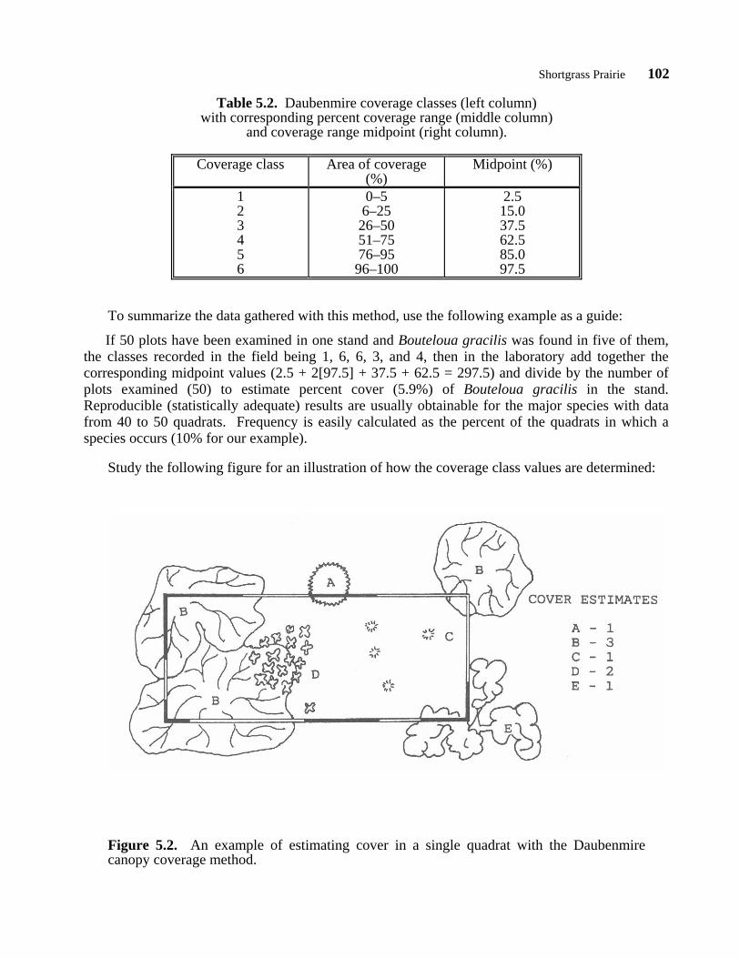
Table 5.2. Daubenmire coverage classes (left column) with corresponding percent coverage range (middle column) and coverage range midpoint (right column).

Coverage class Area of coverage (%)

Midpoint (%)

1 2 3 4 5 6

0–5 6–25 26–50 51–75 76–95 96–100

2.5 15.0 37.5 62.5 85.0 97.5

To summarize the data gathered with this method, use the following example as a guide:

If 50 plots have been examined in one stand and Bouteloua gracilis was found in five of them, the classes recorded in the field being 1, 6, 6, 3, and 4, then in the laboratory add together the corresponding midpoint values (2.5 + 2[97.5] + 37.5 + 62.5 = 297.5) and divide by the number of plots examined (50) to estimate percent cover (5.9%) of Bouteloua gracilis in the stand. Reproducible (statistically adequate) results are usually obtainable for the major species with data from 40 to 50 quadrats. Frequency is easily calculated as the percent of the quadrats in which a species occurs (10% for our example). Study the following figure for an illustration of how the coverage class values are determined:

Figure 5.2. An example of estimating cover in a single quadrat with the Daubenmire canopy coverage method.

103 Shortgrass Prairie As noted previously, the Daubenmire canopy coverage method is most widely used in low vegetation, such as shortgrass prairie or in forest understory where short plants predominate. The method could be adapted for larger plants by enlarging the frame. Another alternative is to simply estimate the percent cover of each species in each quadrat, thereby avoiding the use of coverage class values. In this case, percent cover is the average value from all of the quadrats included in the sample. Quadrats in which the species did not occur are included as zero values. The advantage of using coverage class values is less sampling time and, presumably, greater reproducibility of the cover estimate. Regardless of the approach, estimating cover with the quadrat method requires a visual estimate that may vary from one investigator to another. More precise estimates can be obtained using either the point-quadrat method or the line-intercept method. These methods may require more time in certain vegetation types, however, and the added level of precision may not be necessary for some research objectives.

Shortgrass Prairie 104

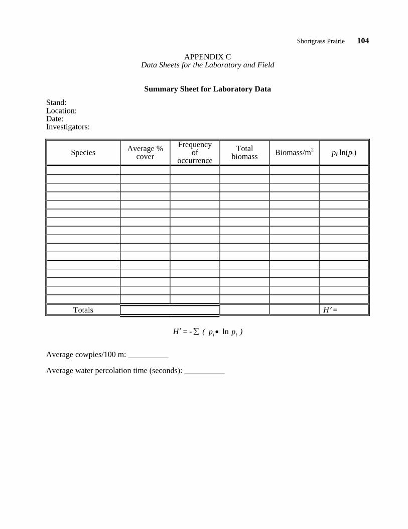
APPENDIX C Data Sheets for the Laboratory and Field Summary Sheet for Laboratory Data

Stand: Location: Date: Investigators:

Species Average % cover

Frequency of

occurrence Total

biomass Biomass/m2 pi⋅ln(pi)

Totals H′ =

Average cowpies/100 m: __________ Average water percolation time (seconds): __________

) p p ( - = H ii ln•∑′

105 Shortgrass Prairie

Summary Sheet for Field Data Stand: Location: Date: Investigators:

Species Quadrat number 1 2 3 4 5 6 7 8 9 10 11 12 13 14 15 16 17 18 19 20

Andropogon smithii* Bouteloua gracilis* Poa sp.* Stipa comata* Oryzopsis hymenoides* Eurotia lanata Carex sp. Sphaeralcea coccinea Afriolet sp. Lichen Opuntia

* Grasses: If seed heads are not clearly visible for identification “lump” grass species together. Comments: