the effects of additive outliers on the seasonal kpss test: a monte carlo analysis

This article was downloaded by: [University of Toronto Libraries]On: 11 August 2014, At: 11:29Publisher: Taylor & FrancisInforma Ltd Registered in England and Wales Registered Number: 1072954 Registeredoffice: Mortimer House, 37-41 Mortimer Street, London W1T 3JH, UK

Journal of Statistical Computation andSimulationPublication details, including instructions for authors andsubscription information:http://www.tandfonline.com/loi/gscs20

The effects of additive outliers onthe seasonal KPSS test: a Monte CarloanalysisSami Khedhiri a & Ghassen El Montasser ba Department of Mathematics and Statistics , University of PrinceEdward Island , Charlottetown, Canadab Department of Economics , University of Manouba , TunisiaPublished online: 05 Mar 2009.

To cite this article: Sami Khedhiri & Ghassen El Montasser (2010) The effects of additive outliers onthe seasonal KPSS test: a Monte Carlo analysis, Journal of Statistical Computation and Simulation,80:6, 643-651, DOI: 10.1080/00949650902755160

To link to this article: http://dx.doi.org/10.1080/00949650902755160

PLEASE SCROLL DOWN FOR ARTICLE

Taylor & Francis makes every effort to ensure the accuracy of all the information (the“Content”) contained in the publications on our platform. However, Taylor & Francis,our agents, and our licensors make no representations or warranties whatsoever as tothe accuracy, completeness, or suitability for any purpose of the Content. Any opinionsand views expressed in this publication are the opinions and views of the authors,and are not the views of or endorsed by Taylor & Francis. The accuracy of the Contentshould not be relied upon and should be independently verified with primary sourcesof information. Taylor and Francis shall not be liable for any losses, actions, claims,proceedings, demands, costs, expenses, damages, and other liabilities whatsoever orhowsoever caused arising directly or indirectly in connection with, in relation to or arisingout of the use of the Content.

This article may be used for research, teaching, and private study purposes. Anysubstantial or systematic reproduction, redistribution, reselling, loan, sub-licensing,systematic supply, or distribution in any form to anyone is expressly forbidden. Terms &

http://www.tandfonline.com/loi/gscs20

http://www.tandfonline.com/action/showCitFormats?doi=10.1080/00949650902755160

http://dx.doi.org/10.1080/00949650902755160

Conditions of access and use can be found at http://www.tandfonline.com/page/terms-and-conditions

Dow

nloa

ded

by [

Uni

vers

ity o

f T

oron

to L

ibra

ries

] at

11:

29 1

1 A

ugus

t 201

4

http://www.tandfonline.com/page/terms-and-conditions

http://www.tandfonline.com/page/terms-and-conditions

Journal of Statistical Computation and SimulationVol. 80, No. 6, June 2010, 643–651

The effects of additive outliers on the seasonal KPSS test:a Monte Carlo analysis

Sami Khedhiria* and Ghassen El Montasserb

aDepartment of Mathematics and Statistics, University of Prince Edward Island, Charlottetown, Canada;bDepartment of Economics, University of Manouba, Tunisia

(Received 19 September 2008; final version received 16 January 2009 )

This article builds on the test proposed by Lyhagen [The seasonal KPSS statistic, Econom. Bull. 3 (2006),pp. 1–9] for seasonal time series and having the null hypothesis of level stationarity against the alternativeof unit root behaviour at some or all of the zero and seasonal frequencies. This new test is qualified asseasonal-frequency Kwiatkowski–Phillips–Schmidt–Shin (KPSS) test and it is not originally supported bya regression framework.

The purpose of this paper is twofold. Firstly, we propose a model-based regression method and providea clear illustration of Lyhagen’s test and we establish its asymptotic theory in the time domain. Secondly,we use the Monte Carlo method to study the finite-sample performance of the seasonal KPSS test in thepresence of additive outliers. Our simulation analysis shows that this test is robust to the magnitude andthe number of outliers and the statistical results obtained cast an overall good performance of the testfinite-sample properties.

Keywords: seasonal KPSS test; additive outliers; Monte Carlo simulation

JEL Classification: C12; C22

1. Introduction

Since the seminal paper of Nelson and Plosser [1], researchers have developed various alternativeunit root models. But the most popular methodologies, at least in empirical work, still rely onunit root tests for which the null hypothesis is the unit root while the alternative is a stationaryprocess.

Nevertheless, this type of test can lead to serious problems because traditional unit root tests arebased on the null hypothesis of a unit root, which assures that this hypothesis will not be rejectedat some significance level unless there is strong evidence against it. Diebold and Rudebush [2]and Bierens [3] show that these tests suffer from low power against alternatives close to the null.

In this paper, we only focus on a unit root test developed by Kwiatkowski–Phillips–Schmidt–Shin [4] hereafter, KPSS, and which is based on the null hypothesis of stationarity. This test hasgained popularity in the economic literature.

*Corresponding author. Email: [email protected]

ISSN 0094-9655 print/ISSN 1563-5163 online© 2010 Taylor & FrancisDOI: 10.1080/00949650902755160http://www.informaworld.com

Dow

nloa

ded

by [

Uni

vers

ity o

f T

oron

to L

ibra

ries

] at

11:

29 1

1 A

ugus

t 201

4

644 S. Khedhiri and G. El Montasser

The economic series are often observed at a higher frequency than the annual. The use ofseasonally unadjusted data is increasingly chosen in empirical applications. As many data ineconomics display trends and unveil stochastic seasonality, several seasonal unit root tests wereestablished over the last two decades. We can refer among others to the Dickey et al. [5], theOsborn et al. [6], the Hylleberg et al. [7] and the Kunst [8] tests. The same problem mentionedabove is also underlined for these tests that are subject to loss of power against alternatives closeto the null; see, inter alia [9]. In practice, seasonal data often exhibit irregularities, abrupt changesand interruptions referred to as outliers, in particular the additive outliers (AO). Measurementerrors or economic, political and financial events can give rise to such AO that affect observationsin isolation. The large and finite-sample effects of these anomalies on seasonal unit root tests havebeen investigated by Haldrup et al. [10].

Lyhagen [11] extended the KPSS framework to the seasonal case and established its limit theorybased on the results of Johansen and Schaumburg [12] and the continuous mapping theorem.Therefore, the resulting test can be termed as seasonal KPSS test.

In this article, we use a model-based regression to compute the test statistics. This enables usto have a simple illustration and a better understanding of the test’s limit theory. Motivated bythe results of Darné [13], who showed that the conventional KPSS test is very robust to AO, weanalyse the effects of these aberrant observations on Lyhagen’s test via simulation study.

The article is organized as follows. In Section 2 we begin with the original formulation ofthe seasonal KPSS test and we describe its asymptotic distribution using an alternative approachbased on the time domain. In Section 3, we allow for possible serial correlation of the errors andin this case, we use Monte Carlo simulations to study the power and size properties of the test infinite samples. In Section 4, we also use Monte Carlo method to assess the effects of AO on thetest. We conclude our findings in Section 5.

2. Seasonal KPSS test

In this section, we present the seasonal KPSS test and its limit theory for unit roots at the seasonalfrequencies. We begin the presentation with the unit root of −1 and to target explicitness, weconsider a quarterly data denoted by yt . We test a negative unit root corresponding to the Nyquistfrequency π as follows:

yt = c + αyt−1 + ut , t = 1, . . . , T , (1)

where c is a constant and (ut ) is i.i.d. (0, σ 2u ).

The null hypothesis of the KPSS test is α = 0, which implies that yt = c + ut is seriallyuncorrelated process with mean equals to c whereas the alternative is α = −1. In order to computethe asymptotic distribution of the test in the case of a negative unit root, we make use of thepartial sum of the demeaned seriesS1,t = ∑t

j=1 (−1)j yj , where yt = yt − y, and we write the teststatistic as follows:

η(−1) = T −2

σ 2u

T∑t=1

(S1,t )2, (2)

where σ 2u is the ordinary least square estimator of the residual variance obtained from Equation (1).

The test η(−1) for the negative unit root has the same asymptotic distribution as the standardtest of a positive unit root with no deterministic terms, namely:

η(−1) =⇒∫ 1

0B2(r) dr, (3)

Dow

nloa

ded

by [

Uni

vers

ity o

f T

oron

to L

ibra

ries

] at

11:

29 1

1 A

ugus

t 201

4

Journal of Statistical Computation and Simulation 645

where ‘⇒’ signifies weak convergence in distribution and B(r) is a Brownian motion withr ∈ [0, 1]. It is well known that the asymptotic distribution of η(−1) is a different member ofthe Cramer-von Mises family; see [14]. The critical values of this distribution can be found in[15–17]. Next, we continue the development of the seasonal KPSS test for the pair of complexunit roots (±i), which correspond to the harmonic seasonal frequencies π/2 and 3π/2. For that,we define the corresponding equation from which the statistic is constructed as follows:

yt = c + αyt−2 + vt , t = 1, . . . , T , (4)

where vt is i.i.d. (0, σ 2v ). To establish the limit theory of the seasonal KPSS in the case of complex

unit roots, we follow the same method as in [18].Let yt be a seasonal process with periodicity s = 2 and with initial values y0 = 0 and y−1 = 0.

Further, assume that we observe Nyears and s = 2 seasons. As such, Equation (5) implies,

yin = c + αyi,n−1 + vin, (5)

where i = 1, 2; n = 1, . . . , N and T = sN. It should be mentioned that in this case there are twoindependent non-stationary processes. To determine the asymptotic distributional result for η(±i)

which is the KPSS test computed with complex unit roots, it will be convenient to rewrite thefunctional central limit theorem as follows:

T −0.5[rT ]∑t=1

(vt − v) = s−0.5N−0.5s∑

i=1

[rN ]∑n=1

(vin − vi )

=⇒ 2−0.5σv

2∑i=1

Bi(r), (6)

where Bi(r) is a Brownian motion and i = 1, 2. Recall that these processes are independent andusing the continuous mapping theorem, we can easily show the following limit result:

η(±i) = T −2

σ 2v

T∑t=1

(S2,t )2 =⇒ 1

2

[∫ 1

0B2

1 (r)dr +∫ 1

0B2

2 (r)dr

], (7)

where B1(r) and B2(r) are two independent Brownian Bridges, S2,t = ∑si=1

∑tj−1 (−1)j yij ,

yij = yj − yi .Consequently, we obtain the same results as in [11] while staying in the time domain. In fact

the test of Lyhagen is qualified as seasonal-frequency KPSS test (see [19]).

3. Serial correlation

The i.i.d. assumption on the error terms in Equations (1) and (4) is somewhat restrictive since therelated processes under the null are also i.i.d. However, we use this assumption for two reasons.First, it helps us to easily find the asymptotic theory of the seasonal KPSS test while staying intime domain by using the double subscript notation for the complex unit roots. Second, becauseof convenience and common practice, the error terms are often assumed to be i.i.d. or n.i.d. inunit root tests. In fact, this makes the search for the limit distributions easier. In this article, weallow for possible serial correlation in the errors that are assumed to be autoregressive (AR) (p)

Dow

nloa

ded

by [

Uni

vers

ity o

f T

oron

to L

ibra

ries

] at

11:

29 1

1 A

ugus

t 201

4


processes and having all the characteristic equation roots outside the unit circle. Further, we definethe moments of ut as follows (the moments of vt are defined in the same way):

E(ut ) = 0,

E(utut−h) = γh,

where the long-run variance of ut is ω2u = ∑+∞

h=−∞ γh, and ω2u > 0.

The Bartlett kernel estimator of ω2u is given by:

ω2u = T −1

T∑t=1

y2t + 2T −1

l∑k=1

w(k, l)

T∑t=k+1

yt yt−k. (8)

With w(k, l) is a weight function such that w(k, l) = 1 − k/(l + 1) and the lag truncation param-eter l verifies l → ∞ when T → ∞ and l = o(n1/2). Andrews [20] showed that such a truncationlag produces good results in practice. For the choice of the values of this parameter, we refer to thethree functions of T used in [4]. We make the following parameter setting: l4 = int[4(T /100)1/4]and l12 = int[12(T /100)1/4], where int[.] denotes the integer part of the expression.

It can be shown that under more general assumptions than autoregressive form of the autocor-relation for ut and vt , respectively, in Equations (1) and (4), the asymptotic results (3) and (7) stillhold.

To assess the size properties of the seasonal KPSS statistic, we conduct Monte Carlo simulationexperiments with the seasonal roots of a quarterly process. The data-generating process (DGP)is Equations (1) and (4) for, respectively, the negative unit root and the complex unit roots ±i.In our simulations, we set the probability distribution of the error terms ut and vt to a standardnormal and we choose alternative values of α ∈ {−1, −0.9, −0.8, 0, 0.1, 0.9}. The choice of ourbandwidth parameter setting is l0, l4 and l12 as defined above.

The results in Table 1 show that decreasing values of α increase the test size. We also noticethat larger data samples do not affect significantly the test size, except for α = 0.1. As pointed byLyhagen [11], our simulations showed that in contrast to the ordinary KPSS framework, l4 and l12do not have, for the most part, better size performance than that of l0. The problem for the ordinaryKPSS test is that by correcting the size, most power is lost. Nevertheless, in the seasonal KPSS

Table 1. Rejection frequencies of the seasonal KPSS test for seasonal quarterly unit roots.

η(−1) η(±i)

α T l0 l4 l12 l0 l4 l2

−1 80 98.99 100 100 99.81 100 100200 99.80 100 100 100 100 100

−0.9 80 80.61 99.45 99.75 93.87 99.93 99.95200 84.27 99.77 99.98 96.84 100 100

−0.8 80 62.02 95.31 97.52 82.02 99.05 99.53200 64.57 96.56 98.97 78.07 98.75 99.94

0 80 5.27 6.96 10.33 5.40 8.32 14.40200 5.39 6.12 8.05 5.14 6.53 9.45

0.1 80 3.17 3.10 5.28 2.87 3.87 7.18200 3.27 2.42 3.37 2.49 2.28 3.53

0.9 80 0.00 0.00 0.00 0.00 0.00 0.00200 0.00 0.00 0.00 0.00 0.00 0.00

Note: The 5% asymptotic critical values are 1.65 and 1.312 for the root −1 and the complex roots ±i as indicated in [1].

Dow

nloa

ded

by [

Uni

vers

ity o

f T

oron

to L

ibra

ries

] at

11:

29 1

1 A

ugus

t 201

4


framework, this characteristic is excluded when the poor size performance induces substantialpower.

In addition, Table 1 results cast an overall good power performance of the seasonal KPSS test,particularly against near seasonal unit root alternatives.

4. Assessment of the effects of AO

Econometricians have studied carefully the impact of AO on unit roots tests. These anomaliescan arise from a combination of factors. Some of these factors are related to data issues, otherfactors may be attributed to natural disasters, which would make the analysis of statistical dataerroneous since the critical values are very sensitive to these shocks and to their timing and size.In this context and based on a univariate analysis, Franses and Haldrup [21] and Shin et al. [22]showed that the presence of AO may have serious effects on the asymptotic distribution of theDickey–Fuller (DF) statistics. For the most part, the DF test under AO tends to over-reject the nullhypothesis of unit root in favour of the stationary alternative. More recently, Haldrup et al. [10]showed the impact of these anomalies on seasonal unit roots in a more general context such thatof measurement errors.

We now describe our Monte Carlo experiments designed to assess the finite-sample propertiesof the seasonal KPSS test statistics. The DGP are given by Equations (1) and (4) for the negativeunit root and for the complex unit roots with α ∈ {0, −1} and ut and vt are normally distributedwith zero mean and unit variance. Since AO are viewed as rare events, we allow the contaminationof the DGP as follows:

(i) single AO at k = T/2;(ii) two AO at k = 2T/5 and 4T/5;

(iii) three AO at k = 2T/5, T /2 and 4T/5.

The magnitude ξ of AO takes the values between 3 and 7, which are relatively the smallest and thebiggest values of those used in other studies; see, for example, [23,24]. The sample size is T = 80and 200 and all experiments are based on 20,000 replications. Cases (i)–(iii) were investigated byDarné [13] who showed that standard KPSS test is robust to AO.

4.1. Seasonal KPSS test for the root −1

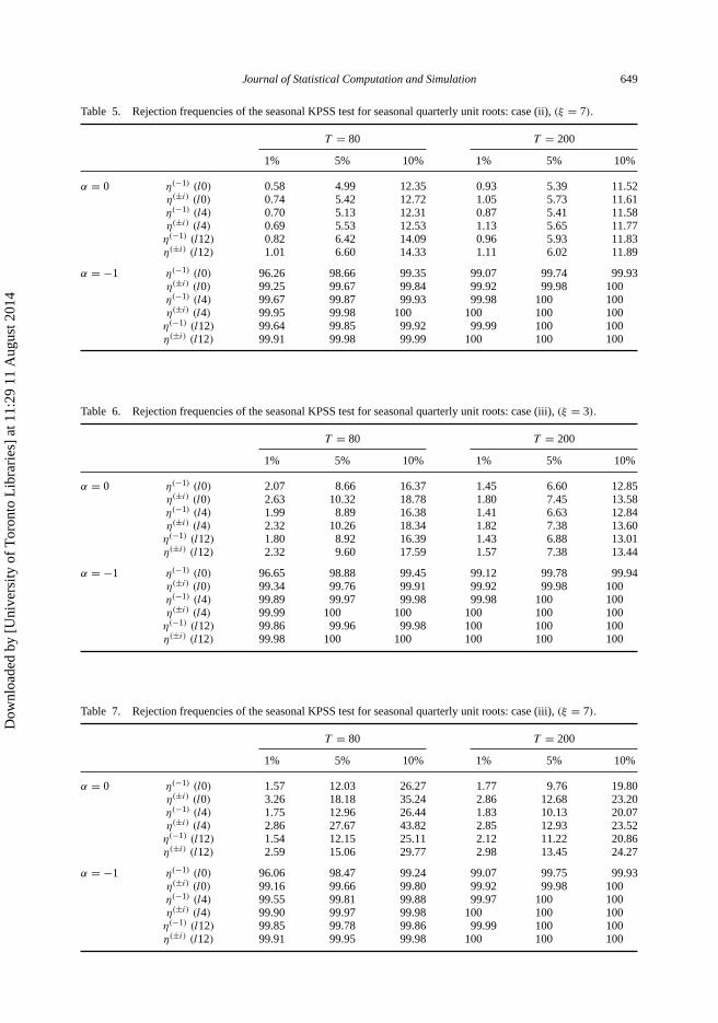
From Tables 2–7, we can draw the following results. In the case of one AO with magnitude ξ = 3,

the test shows almost no change in size, but when the magnitude becomes 7, η(−1) becomes slightlyundersized for the 1% and 5% quantiles. In this situation and compared with ξ = 3, the powerof the test is reduced just very slightly. This may not affect the overall test power performance.With two AO, it is noticed that when the magnitude changes from 3 to 7, the test becomes slightlyundersized for the 1% quantile, but for the other quantiles it is somewhat oversized.

It is also worth mentioning that the change in magnitude has very little effect on the test power.In fact with ξ = 3, the power shows just a small reduction. When we compare this scenario withcase (ii), it can be concluded that the realization of another AO inflates the test size.

Now in comparison to case (ii), case (iii) proves that the real size of the test η(−1) exceedsremarkably the nominal levels and in several times the test is considerably oversized, especiallyat the 10% level. Moreover, the increase in the magnitude of the outliers generates increase in thesize of the test. What looks like an exception is the case for the 1% quantile with T = 80.

Dow

nloa

ded

by [

Uni

vers

ity o

f T

oron

to L

ibra

ries

] at

11:

29 1

1 A

ugus

t 201

4


Table 2. Rejection frequencies of the seasonal KPSS test for seasonal quarterly unit roots: case (i), ξ = 3.

T = 80 T = 200

1% 5% 10% 1% 5% 10%

α = 0 η(−1)(l0) 1.01 4.96 10.18 0.94 4.98 10.21η(±i)(l0) 1.00 5.04 10.21 1.06 5.02 9.74η(−1)(l4) 1.00 5.07 10.10 0.94 4.96 10.04η(±i)(l4) 1.00 5.01 9.88 1.03 4.94 9.89η(−1)(l12) 0.93 5.10 10.36 1.37 5.06 10.11η(±i)(l12) 1.08 5.00 10.22 0.94 4.92 10.01

α = −1 η(−1)(l10) 96.76 98.95 99.45 99.13 99.79 99.94η(±i)(l0) 99.38 99.77 99.90 99.93 99.98 100η(−1)(l4) 99.92 99.98 99.99 100 100 100η(±i)(l4) 100 100 100 100 100 100η(−1)(l12) 99.89 99.98 99.99 100 100 100η(±i)(l12) 99.98 100 100 100 100 100

Note: η(−1)and η(±i)(l) are defined in Equations (2) and (7).η(−1) (l) and η(±i)(l) show that the variance estimators are replaced by spectral density estimators with bandwidth l ∈ {l0, l4, l12} asdescribed in the text.

Table 3. Rejection frequencies of the seasonal KPSS test for seasonal quarterly unit roots: case (i), (ξ = 7).

T = 80 T = 200

1% 5% 10% 1% 5% 10%

α = 0 η(−1) (l0) 0.70 4.53 10.20 0.86 4.73 10.17η(±i) (l0) 0.66 4.33 9.75 0.93 4.86 9.93η(−1) (l4) 0.69 4.57 10.01 0.83 4.90 10.11η(±i) (l4) 0.63 4.33 9.46 0.94 4.91 9.95η(−1) (l12) 0.69 4.63 10.15 0.91 4.99 10.06η(±i) (l2) 0.85 4.47 9.78 0.90 4.78 9.78

α = −1 η(−1) (l0) 96.49 98.82 99.42 99.12 99.78 99.94η(±i) (l0) 99.30 99.73 99.89 99.78 99.92 99.98η(−1) (l4) 99.80 99.92 99.96 99.98 100 100η(±i) (l4) 99.98 99.99 100 100 100 100η(−1) (l2) 99.74 99.92 99.97 100 100 100η(±i) (l12) 99.97 99.98 100 100 100 100

Table 4. Rejection frequencies of the seasonal KPSS test for seasonal quarterly unit roots: case (ii), (ξ = 3).

T = 80 T = 200

1% 5% 10% 1% 5% 10%


α = −1 η(−1) (l0) 96.73 98.92 99.46 99.12 99.79 99.94η(±i) (l0) 99.34 99.76 99.91 99.93 99.98 100η(−1) (l4) 99.90 99.97 99.98 99.98 100 100η(±i) (l4) 100 100 100 100 100 100η(−1) (l12) 99.88 99.98 99.99 100 100 100η(±i) (l12) 100 100 100 100 100 100

Dow

nloa

ded

by [

Uni

vers

ity o

f T

oron

to L

ibra

ries

] at

11:

29 1

1 A

ugus

t 201

4


Table 5. Rejection frequencies of the seasonal KPSS test for seasonal quarterly unit roots: case (ii), (ξ = 7).

T = 80 T = 200

1% 5% 10% 1% 5% 10%


α = −1 η(−1) (l0) 96.26 98.66 99.35 99.07 99.74 99.93η(±i) (l0) 99.25 99.67 99.84 99.92 99.98 100η(−1) (l4) 99.67 99.87 99.93 99.98 100 100η(±i) (l4) 99.95 99.98 100 100 100 100η(−1) (l12) 99.64 99.85 99.92 99.99 100 100η(±i) (l12) 99.91 99.98 99.99 100 100 100

Table 6. Rejection frequencies of the seasonal KPSS test for seasonal quarterly unit roots: case (iii), (ξ = 3).

T = 80 T = 200

1% 5% 10% 1% 5% 10%


α = −1 η(−1) (l0) 96.65 98.88 99.45 99.12 99.78 99.94η(±i) (l0) 99.34 99.76 99.91 99.92 99.98 100η(−1) (l4) 99.89 99.97 99.98 99.98 100 100η(±i) (l4) 99.99 100 100 100 100 100η(−1) (l12) 99.86 99.96 99.98 100 100 100η(±i) (l12) 99.98 100 100 100 100 100

Table 7. Rejection frequencies of the seasonal KPSS test for seasonal quarterly unit roots: case (iii), (ξ = 7).

T = 80 T = 200

1% 5% 10% 1% 5% 10%


α = −1 η(−1) (l0) 96.06 98.47 99.24 99.07 99.75 99.93η(±i) (l0) 99.16 99.66 99.80 99.92 99.98 100η(−1) (l4) 99.55 99.81 99.88 99.97 100 100η(±i) (l4) 99.90 99.97 99.98 100 100 100η(−1) (l12) 99.85 99.78 99.86 99.99 100 100η(±i) (l12) 99.91 99.95 99.98 100 100 100

Dow

nloa

ded

by [

Uni

vers

ity o

f T

oron

to L

ibra

ries

] at

11:

29 1

1 A

ugus

t 201

4


4.2. Seasonal KPSS test for complex unit roots

From our simulation results reported in Tables 2–7, we can also draw the following conclusions:In case (i) with increasing magnitude of the AO, the test η(±i) shows little distortion for the 1% and5% quantiles. In fact, and similarly to the results obtained in Section 4.1, this test becomes veryslightly undersized but behaves as expected under the null. We can also notice that while using alarger sample size improves the performance of the test, an increase in the bandwidth parameterwith ξ = 3 and T = 200 worsens the test size performance for both 1% and 5% quantiles.

Observe that in case (ii), the test is clearly oversized at 1% and 5% for ξ = 3. The distortionsare greater for l12 with T = 80. On the other hand, with ξ = 7 and compared with the othervalues of the magnitude of AO, the power of the test decreases slightly but remains very muchappreciable.

Lastly, in case (iii), the test becomes heavily oversized in particular for the 5% and 10%quantiles. We can also notice that the increase in the bandwidth reduces to some extent the size ofthe test with ξ = 3. The increase in the sample size slightly improves the overall test performance.

5. Conclusion

The aim of this article is to provide a more comprehensive representation of the seasonal KPSStest in order to understand the underlying limit theory. It is shown that AO can seriously affectthe seasonal unit root testing. In this respect, we refer to Haldrup et al. [10] who showed thatAO affect the size of the most renowned seasonal unit root test that was introduced by Hylleberget al. [7]. In contrast, the size of the seasonal KPSS test offers some robustness to the magnitudeand the number of these aberrant observations. Furthermore, our simulation results prove thatthe seasonal KPSS test is very promising and shows good power properties. To obtain a moredetailed picture, we may introduce to this test some short dynamics like seasonal dummies. Wethen obtain a test of deterministic seasonality very similar to that of Canova and Hansen [9] andadopting the same framework. In this case, the study of the effects of AO on this test is certainlyinteresting. We will follow this direction in our future research.

References

[1] C.R. Nelson and C.I. Plosser, Trends versus random walks in economic time series: some evidence and implications,J. Monetary Econom. 10 (1982), pp. 139–162.

[2] F.X. Diebold and G.D. Rudebush, On the power of Dickey–Fuller tests against fractional alternatives, Econom.Lett. 35 (1991), pp. 155–160.

[3] H.J. Bierens, Topics in Advanced Econometrics, Cambridge University Press, Cambridge, 1994.[4] D. Kwiatkowski, P.C.B. Phillips, P. Schmidt, and Y. Shin, Testing the null of stationarity against the alternative of

a unit root: how sure are we that economic time series have a unit root? J. Econometrics 54 (1992), pp. 159–178.[5] D.A. Dickey, D.P. Hasza, and W.A. Fuller, Testing for unit roots in seasonal time series, J. Amer. Statist. Assoc. 79

(1984), pp. 355–367.[6] D.R. Osborn,A.P.L. Chui, J.P. Smith, and C.R. Birchenhall, Seasonality and the order of integration for consumption,

Oxford Bull. Econom. Statist. 50 (1988), pp. 361–377.[7] S. Hylleberg, R.F. Engle, C.W.J. Granger, and B.S. Yoo, Seasonal integration and cointegration, J. Econometrics 44

(1990), pp. 215–238.[8] R.M. Kunst, Testing for cyclical non-stationarity in autoregressive processes, J. Time Ser. Anal. 18 (1997),

pp. 123–135.[9] F. Canova and B.E. Hansen, Are seasonal patterns constant over time? A test for seasonal stability, J. Bus. Econom.

Statist. 13 (1995), pp. 237–252.[10] N. Haldrup, A. Montanés, and A. Sanso, Measurement errors and outliers in seasonal unit root testing,

J. Econometrics 127 (2005), pp. 103–128.[11] J. Lyhagen, The seasonal KPSS statistic, Econom. Bull. 3 (2006), pp. 1–9.[12] S. Johansen and E. Schaumburg, Likelihood analysis of seasonal cointegration, J. Econometrics 54 (1998),

pp. 159–178.

Dow

nloa

ded

by [

Uni

vers

ity o

f T

oron

to L

ibra

ries

] at

11:

29 1

1 A

ugus

t 201

4


[13] O. Darné, The effects of additive outliers on stationarity tests: a Monte Carlo study, Econom. Bull. 3 (2004), pp. 1–8.[14] F. Busetti and A.C. Harvey, Testing for trend, Econom. Theory 24 (2007), pp. 72–87.[15] I. McNeill, Properties of sequences of partial sums of polynomial regression residuals with applications to tests for

change of regression at unknown times, Ann. Statist. 6 (1978), pp. 422–433.[16] J. Nyblom, Testing for the constancy of parameters over time, J. Amer. Statist. Assoc. 84 (1989), pp. 223–230.[17] B. Hobijn and P.H. Franses, Asymptotically perfect and relative convergence of productivity, J. Appl. Econometrics

15 (2000), pp. 59–81.[18] E. Ghysels and D.R. Osborn, The Econometric Analysis of Seasonal Time Series, Cambridge University Press,

Cambridge, 2001.[19] F. Busetti and A.C. Harvey, Testing against stochastic seasonality, Mimeo, 2000.[20] D.W.K. Andrews, Heteroskedasticity and Autocorrelation Consistent Covariance Matrix Estimation, Econometrica

59 (1991), pp. 817–858.[21] P.H. Franses and N. Haldrup, The effects of additive outliers on tests for unit roots and cointegration, J. Bus. Econom.

Statist. 12 (1994), pp. 471–478.[22] D.W. Shin, S. Sarkar and J.H. Lee, Unit root tests for time series with outliers, Statist. Probab. Lett. 30 (1996),

pp. 189–197.[23] P.H. Franses and H. Ghijsels, Additive outliers, GARCH and forecasting volatility, Int. J. Forecast.15 (1999), pp. 1–9.[24] J. Tolvi, The effects of outliers on two nonlinear tests, Comm. Statist. Simulation Comput. 29 (2000), pp. 897–918.

Dow

nloa

ded

by [

Uni

vers

ity o

f T

oron

to L

ibra

ries

] at

11:

29 1

1 A

ugus

t 201

4

the effects of additive outliers on the seasonal kpss test: a monte carlo analysis

Documents