the effective dose of different scanning protocols using

Western University Western University

Scholarship@Western Scholarship@Western

Electronic Thesis and Dissertation Repository

12-2-2013 12:00 AM

The Effective Dose of Different Scanning Protocols Using the The Effective Dose of Different Scanning Protocols Using the

Sirona Galileos® Comfort CBCT Scanner Sirona Galileos® Comfort CBCT Scanner

David R. Chambers, The University of Western Ontario

Supervisor: Dr. Richard Bohay, The University of Western Ontario

Joint Supervisor: Dr. Jerry Battista, The University of Western Ontario

A thesis submitted in partial fulfillment of the requirements for the Master of Clinical Science

degree in Orthodontics

© David R. Chambers 2013

Follow this and additional works at: https://ir.lib.uwo.ca/etd

Part of the Other Dentistry Commons

Recommended Citation Recommended Citation Chambers, David R., "The Effective Dose of Different Scanning Protocols Using the Sirona Galileos® Comfort CBCT Scanner" (2013). Electronic Thesis and Dissertation Repository. 1877. https://ir.lib.uwo.ca/etd/1877

This Dissertation/Thesis is brought to you for free and open access by Scholarship@Western. It has been accepted for inclusion in Electronic Thesis and Dissertation Repository by an authorized administrator of Scholarship@Western. For more information, please contact [email protected].

https://ir.lib.uwo.ca/

https://ir.lib.uwo.ca/etd

https://ir.lib.uwo.ca/etd?utm_source=ir.lib.uwo.ca%2Fetd%2F1877&utm_medium=PDF&utm_campaign=PDFCoverPages

http://network.bepress.com/hgg/discipline/661?utm_source=ir.lib.uwo.ca%2Fetd%2F1877&utm_medium=PDF&utm_campaign=PDFCoverPages

https://ir.lib.uwo.ca/etd/1877?utm_source=ir.lib.uwo.ca%2Fetd%2F1877&utm_medium=PDF&utm_campaign=PDFCoverPages

mailto:[email protected]

THE EFFECTIVE DOSE OF DIFFERENT SCANNING PROTOCOLS USING THE SIRONA GALILEOS® COMFORT CBCT SCANNER

(Thesis format: Monograph)

by

David Chambers

Graduate Program in Orthodontics

A thesis submitted in partial fulfillment of the requirements for the degree of

Master of Clinical Dentistry

The School of Graduate and Postdoctoral Studies The University of Western Ontario

London, Ontario, Canada

© David Chambers 2014

ii

Abstract

Introduction: Cone Beam CT imaging is prevalent in dentistry yet much is unknown with

regard to how radiation dose to the patient varies between different CBCT scanners and

imaging protocols. Scanner and protocol specific effective dose calculations will aid in

optimizing individualized protocols for clinical applications.

Purpose: To determine the effective dose for a range of imaging protocols using the Sirona

GALILEOS Comfort CBCT scanner.

Materials and Methods: Calibrated InLight nanoDot OSL dosimeters (Landauer,

Glenwood, Ill) were placed at 26 select sites in the head and neck of a modified, human

tissue-equivalent RANDO phantom. Effective dose was calculated using the measured local

absorbed doses, accounting for the fractional volume and type of tissue exposed, and

applying the 2007 ICRP1 tissue weighting factors. In total, 12 different scanning protocols

were investigated varying the field of view, mAs, contrast and resolution parameters.

Results: The effective doses for a repeated protocol (full maxillomandibular scan, maximum

(42) mAs, high contrast and resolution) were 140, 141 and 142 µSv. This compares to 100

µSv for a maxillary scan and 107 µSv for a mandibular scan with identical mAs, contrast and

resolution settings. Effective dose remained between 140-142 µSv for maxillomandibular

scans at 42 mAs with varying contrast and resolution settings.

Conclusions: Changes to mAs and beam collimation have a significant influence on

effective dose. Effective dose varies linearly with mAs. Collimating to obtain a narrower

maxillary or mandibular scan decreases effective dose by approximately 28% and 23%

respectively as compared to a full maxillomandibular scan. Changes to contrast and

resolution settings have little influence on effective dose. This study provides data for setting

individualized patient exposure protocols in order to minimize patient dose from ionizing

radiation used for diagnostic or treatment planning tasks in dentistry

Keywords: dosimetry, radiation dosage, effective dose, cone beam computed tomography,

CBCT

iii

Co-Authorship Statement

This study was the result of a collaborative effort among several individuals. Completion of

this thesis was not possible without their important contributions.

David Chambers – wrote thesis, study design, data collection and analysis

Dr. Richard N. Bohay – supervisor, reviewed thesis, study design and analysis

Dr. Jerry Battista (Biophysics) – advisor, study design and analysis, thesis editing

Linada Kaci (Biophysics) – reviewed thesis, study design, data collection and error analysis,

dose calibration of OSL dosimeters

Dr. Rob Barnett (Biophysics) – study design and analysis, provided access to dosimetry

equipment and calibration x-ray beam of the London Regional Cancer Program, London

Health Sciences Centre

iv

Acknowledgments

I would like to express my sincere appreciation to all of those who made important

contributions in completing this project.

I wish to thank my co-supervisors Dr. Richard Bohay and Dr. Jerry Battista. Your

enthusiasm, insight and genuine interest made for a positive research experience. I was

fortunate to receive your combined guidance.

This project would not have been possible without the valuable assistance of Linada Kaci.

Her willingness to provide much of her time despite many clinic responsibilities was greatly

appreciated. I could not have asked for a better research partner.

A very special thank you to Dr. Antonios Mamandras, Dr. Ali Tassi, Dr. John Murray and

Dr. Jeff Dixon for recognizing my desire to study this specialty and extending me that

privilege. I will always be grateful.

Thank you to all of the full-time and part-time faculty members for your dedication to this

profession in providing your time to enhance my professional and academic development.

To Jo Ann Pfaff, Barb Merner, Evelyn Larios, Patricia Vanin and Jacquie Geneau, thank you

for all your continued assistance and support, the clinic is fortunate to have such a great team.

To my fellow residents, past and current, I was fortunate to spend my time with such an

amazing group of individuals. To my classmates Natalie Swoboda and Bhavana Sawhney,

thanks for the laughs and continued encouragement. I am grateful for the opportunity to

have shared this experience with you.

Finally, a sincere thank you to my parents and loved ones for your continued support in

realizing my academic goals. Accomplishing them was a direct result of your influence and

encouragement.

v

Table of Contents

Abstract ............................................................................................................................... ii

Co-Authorship Statement................................................................................................... iii

Acknowledgments.............................................................................................................. iv

Table of Contents ................................................................................................................ v

List of Tables .................................................................................................................... vii

List of Figures .................................................................................................................. viii

List of Appendices ............................................................................................................. ix

List of Abbreviations .......................................................................................................... x

INTRODUCTION .............................................................................................................. 1

BACKGROUND ................................................................................................................ 3

X-Radiation .................................................................................................................... 3

Dental Radiology: History ............................................................................................. 3

Development ........................................................................................................... 3

Dental Radiographic Techniques ............................................................................ 4

The Biologic Effects of Radiation................................................................................ 11

Radiation Dosimetry .................................................................................................... 12

Exposure ............................................................................................................... 12

Absorbed Dose ...................................................................................................... 12

Equivalent Dose .................................................................................................... 13

Effective Dose ....................................................................................................... 14

Experimental Dosimetry Methods ........................................................................ 15

Dosimeters ............................................................................................................ 16

CBCT Protocol Parameters .......................................................................................... 18

Field of View ........................................................................................................ 18

vi

Scan Time ............................................................................................................. 18

Exposure Time ...................................................................................................... 19

CBCT Voxel Size ................................................................................................. 19

Sirona GALILEOS® Parameters .......................................................................... 19

PURPOSE ......................................................................................................................... 21

MATERIALS AND METHODS ...................................................................................... 22

Dosimeters ................................................................................................................... 22

Phantom ....................................................................................................................... 23

Anatomic Landmarks ................................................................................................... 25

Phantom Orientation .................................................................................................... 27

Protocols ....................................................................................................................... 29

RESULTS ......................................................................................................................... 32

DISCUSSION ................................................................................................................... 36

SUMMARY ...................................................................................................................... 42

CONCLUSIONS............................................................................................................... 43

REFERENCES ................................................................................................................. 44

APPENDICES .................................................................................................................. 50

CURRICULUM VITAE ................................................................................................... 56

vii

List of Tables

Table 1: Effective dose estimates for common dental radiographs ........................................ 10

Table 2: Radiation weighting factors recommended by ICRP ............................................... 13

Table 3: Tissue weighting factors as recommended by ICRP (2007) .................................... 14

Table 4: Comparison of TLD and OSLD properties .............................................................. 17

Table 5: Anatomic sites for dosimeter placement................................................................... 25

Table 6: Summary of protocols investigated .......................................................................... 29

Table 7: Percentage tissue irradiated, tissue weighting factor and OSLD sample for each

tissue/organ ............................................................................................................................. 31

Table 8: Effective dose calculations for protocols completed ................................................ 32

Table 9: Effective dose of collimated scans ........................................................................... 33

Table 10: Equivalent dose (µSv) to tissues/organs ................................................................. 34

Table 11: Equivalent doses for maxillary scan as a percentage of equivalent doses for

mandibular scan (taken as mean of percentages for 14, 28 and 42 mAs) ............................... 34

Table 12: Effect of resolution and contrast on dose ............................................................... 35

viii

List of Figures

Figure 1: Sample Image, Sirona GALILEOS® ........................................................................ 8

Figure 2: Available Exposure Settings for GALILEOS® Comfort ........................................ 19

Figure 3: Therapax HF 150 ..................................................................................................... 23

Figure 4: PMMA template for OSLD placement ................................................................... 24

Figure 5: RANDO® phantom with PMMA templates in place ............................................. 24

Figure 6: Relationship of hard and soft tissue in RANDO® phantom ................................... 26

Figure 7: Lateral Cephalometric view with lead foil at OSLD locations .............................. 27

Figure 8: Modified mount for setup reproduction .................................................................. 28

Figure 9: 'Tilt' and 'Rotation', confirming setup reproduced ................................................... 28

Figure 10: High intensity light source to anneal OSL dosimeters .......................................... 30

Figure 11: Effective Dose vs mAs .......................................................................................... 33

ix

List of Appendices

Appendix A: Average OSLD Counts - Full Scan, 42mAs, HC/HR ...................................... 51

Appendix B: Average OSLD Counts - Full Scan, HC/HR .................................................... 52

Appendix C: Average OSLD Counts - Maxillary Scan, HC/HR........................................... 53

Appendix D: Average OSLD Counts – Mandibular Scans, HC/HR ..................................... 54

Appendix E: Average OSLD Counts – Full Scans ................................................................ 55

x

List of Abbreviations

ALARA As Low as Reasonably Achievable

CBCT Cone Beam Computed Tomography

CCD Charge Coupled Device

CMOS Complementary Metal Oxide Semiconductors

CT Computed Tomography

CTDIvol Computed Tomography Dose Index by Volume, accounting for overlap of CT

slices

CTDIW Weighted Computed Tomography Dose Index, averaging dose in a CT slice

DT Absorbed Dose for tissue ‘T’

E Effective Dose – in units of Sievert (see below), a weighted sum of

tissue/organ doses (DT)

EBM Electronic Band Model

FOV Field of View

Gy Gray (unit of Absorbed Dose – 1 J/kg)

HC High Contrast

HR High Resolution

HT Equivalent Dose for tissue ‘T’

HVL Half Value Layer (requirement to attenuate 50% of incident radiation)

ICRP International Commission on Radiological Protection

xi

keV kiloelectronvolts

kV kilovoltage

LET Linear Energy Transfer

mA milliampere (x-ray tube current)

mAs milliampere seconds (product of mA and time)

MDCT Multidetector Computed Tomography

MeV Megaelectronvolts

MV Megavolts

NC Normal Contrast

OSLD Optically Stimulated Luminescence Dosimeter

PKA Air Kerma-Area Product

PKL,CT CT Air Kerma-Length Product

PMMA Polymethyl methacrylate

PSP Photostimulable Phosphor

R Roentgen (unit of radiation exposure)

SR Standard Resolution

Sv Sievert (unit of Effective Dose)

TAD Temporary Anchorage Device

TLD Thermoluminescence Dosimeter

TMJ Temporomandibular Joint

xii

VO1 Volume 1 (High Resolution)

VO2 Volume 2 (Standard Resolution)

WR Radiation Weighting Factor for radiation type ‘R’

1

INTRODUCTION

Dental radiography provides essential information in diagnosis and subsequent treatment

planning. While two-dimensional analog techniques continue to be employed in routine dental

practice, digital and three-dimensional modalities are becoming increasingly common. Digital

radiography offers improved compatibility with practice management and imaging software,

reduces storage needs, eliminates chemical, Silver and lead foil waste, facilitates transfer of

images between practitioners and may offer reduced radiation exposure.2 Three-dimensional

imaging techniques provide a means for interpreting the spatial relationship of structures

otherwise superimposed on standard two-dimensional images. This has important implications

in dental implantology and other surgical procedures where detailed assessment of structures

adjacent to the surgical site is essential. In clinical situations where several two-dimensional

images are indicated, three-dimensional techniques offer an efficient method of reconstructing

the same group of images while limiting image acquisition to a single exposure. 3

While three-dimensional images may offer abundant clinical information, it is not sufficient to

prescribe them on the basis of convenience. Of equal importance in determining which image to

prescribe is the associated radiation exposure incurred by the patient. Haphazard selection of

images that exceed the region of interest and quality required for diagnosis exposes the patient to

undue risk from ionizing radiation. For this reason, guidelines suggest that radiation exposure be

limited to as low as reasonably achievable, with the benefits from the diagnostic information

obtained exceeding the risks incurred by exposure. 4-6

The question of which radiograph to prescribe for a given patient and clinical scenario becomes a

complex one requiring an in depth knowledge of the parameters set at image acquisition and

their respective effects on both diagnostic image quality and patient exposure. Obtaining an

image with maximum field and resolution may provide the most complete set of imaging data for

the patient but at the expense of increased radiation dose. Determination of the appropriate

scanning protocol must be considered in the context of the patient history, clinical findings,

previous imaging results, differential diagnosis and treatment plan. The scanning protocol must

also take into consideration the age and size of the patient as well as the ability of the scan to

demonstrate the anatomy of interest. It becomes obvious that image protocol optimization is not

2

a simple task and prescription requires a thorough knowledge of both diagnostic imaging and the

risks of biologic effects due to ionizing radiation.

The purpose of this study is to investigate the effective radiation dose associated with the Sirona

GALILEOS® Comfort Cone Beam CT scanner using different scanning protocols. An

understanding of the effect of field of view (FOV), milliampere seconds (mAs), contrast and

resolution (voxel size) on effective dose will aid the clinician in determining the optimum

protocol for each patient and clinical question. This study will focus on exposure while it is

understood that image quality is also of importance and will require subsequent study.

3

BACKGROUND

X-Radiation

The x-ray was discovered in 1895 by Bavarian physicist Wilhelm Roentgen.7 Roentgen was

experimenting with cathode rays using a vacuum tube, electrical current and screens that

fluoresced when exposed to radiation when he noticed that screens on an adjacent table were

fluorescing. The screens were several feet away from the vacuum tube, a distance greater than

cathode rays could travel. He therefore concluded that there existed an unknown ray responsible

for these findings and named it the x-ray due to its unknown properties. Roentgen continued to

experiment with x-rays eventually obtaining the first radiograph of the human body, that of his

wife’s hand.7

Dental Radiology: History

Development

With the discovery of the x-ray came interest in dental imaging. In 1895 German dentist Otto

Walkhoff obtained the first dental radiograph of his own mouth.7 Continued experimentation by

several pioneers lead to application on live patients and the development of radiographic

techniques. Boston dentist William Rollins is accredited with the development of the first dental

x-ray unit.7 He introduced interest in radiation protection recognizing the dangers of radiation.

Unfortunately early pioneers were not aware of the associated dangers with many suffering the

effects of overexposure to radiation.

In 1913, William Coolidge developed the first hot-cathode x-ray tube. It consisted of a high-

vacuum tube with a tungsten filament and serves as the prototype for all modern x-ray tubes.

Victory X-Ray Corp. began manufacturing an x-ray machine with a small version of the x-ray

tube within the head in 1923. This design was later superseded by the variable kilovoltage

machine in 1957 with introduction of the recessed long-beam tube head in 1966.7

Initial dental x-ray packets were fabricated from glass photographic plates, wrapped in black

paper and rubber. Eastman Kodak Company began manufacturing pre-wrapped intraoral film in

1913 with the first periapical packets available in 1920. Subsequent improvements in film lead

4

to D-speed film in 1955, E-speed film in 1981 and F-speed film in 2000. Current fast film

requires less than 2% of the exposure required for that available in 1920.

The modern era of digital dental radiography followed Dr. Francis Mouyen’s 1989 paper

describing radiovisiography. 8,9

Multiple advantages have resulted in a shift toward digital

imaging in dentistry including lower patient exposure, ability to transfer images between health

care providers without degradation in image quality and a reduction in chemical, Silver and lead

foil waste associated with analog imaging.2 Two main technologies exist, solid-state technology

and photostimulable phosphor (PSP) technology.2 Solid state detectors function by collecting

the charge produced by x-rays in a solid semiconducting material producing rapid image

availability. 2 Subtypes include charge-coupled devices (CCD), complementary metal oxide

semiconductors (CMOS) and flat panel detectors. Photostimulable phosphor plates absorb

energy from x-rays. Stimulation by appropriate light leads to release of this energy in the form

of visible light and subsequently quantified to measure the amount of x-ray energy absorbed.

Dental Radiographic Techniques

Intraoral

Soon after the discovery of x-rays, dental radiographic techniques began to emerge. Edmund

Kells of New Orleans, with many significant contributions to radiology in North America,

introduced the paralleling technique in 1896 while Weston Price introduced the bisecting

technique in 1904. This was later refined by Howard Raper when introducing the bite-wing

technique in 1925.7 Franklin McCormack began use of the paralleling technique in 1920 and in

1937 published a paper explaining the advantages to the long distance paralleling technique in

minimizing distortion when compared to the bisecting technique.7,10

These advantages were

realized when F. Gordon Fitzgerald introduced the long-cone paralleling technique in 1947.

Extraoral

Cephalometry

Craniometry is described as the art of measuring the skulls of animals and has been documented

for many centuries.11

It provided the foundation for cephalometry which involves measuring the

head inclusive of soft tissue. Documentation of skull form analysis dates back to Hippocrates

5

(460-357BC).11

Leonardo da Vinci (1452-1519) was one of earliest to apply the theory of head

measurement, using a variety of lines relating to head landmarks in order to study human form.11

Craniometry continued to develop in the following centuries during which the craniostat was

developed in recognizing the importance of reproducibility and standardized methods.11

In 1922, A.J. Pacini published a thesis entitled “Roentgen Ray Anthropometry of the Skull” in

which he outlined a procedure for positioning and immobilizing a subjects head such that the

median sagittal plane was parallel to the film.12,13

This was developed for anthropologic

purposes. It was not until 1931 that dentists Hofrath and Broadbent simultaneously published

details on an apparatus, the ‘cephalostat’, used to position the heads of live patients in relation to

the x-ray source and film such that the lateral cephalogram could be obtained.11

Subsequently,

the art and science of cephalometrics developed gaining widespread acceptance for use in

diagnosis, study of growth and development and the effects of treatment.13

Conventional Tomography:

Clinical demand for three-dimensional imaging lead to the development of conventional

tomography with Polish radiologist Mayer first suggesting the idea in 1914.14

This technique is

used to obtain an image of a select plane of tissue while blurring adjacent structures.7 In

conventional film-based tomography, the x-ray tube and film are rigidly connected and

synchronous movement around a fixed axis produces a sharp image layer (‘tomographic layer’)

with adjacent structures outside the focal plane blurred.2 Several types of movement are

possible including linear, circular, elliptic, hypocycloidal and spiral.2

Panoramic

While much utility was recognized in early intraoral techniques, the need for obtaining an

unobstructed view of the maxilla, mandible and dentition was recognized. In 1922, A.F. Zulauf

patented the ‘panoramic x-ray apparatus”, describing a method where a narrow beam scanned

both the upper and lower jaws.15,16

Hisatugu Numata of Japan was the first to expose a

panoramic radiograph in 1933, using a device constructed for clinical examination termed

“parabolic radiography” with the film placed lingual to the dentition.15

Yrjo Paatero of Finland,

considered the ‘father of panoramic radiography’ experimented with slit beam and rotational

6

techniques. He published several papers describing use of the technique in clinical

practice.7,15,17-20

Development of commercial equipment for panoramic radiography began with production of the

Orthopantomograph by Palomex under the charge of Timo Nieminen in 1960.15

Increased

clinical use resulted in progression to large-scale production. Early models of commercial

equipment were controlled by mechanical means. The first publication on computed panoramic

radiography was released by H. Kashima et al of Japan in 1985 with the first electronic system

for rotational panoramic radiography reported by McDavid et al in 1991.21-23

Conventional Computed Tomography (CT)

Computed tomography has undergone continued development since first introduced for clinical

application. Related theory dates back to 1917 when mathematician J.H. Radon proved the

distribution of an x-ray attenuating material in an object layer can be calculated if the integral

values along many ray-lines passing through the same layer are known.24

The Radon transform

provided the mathematical basis for image reconstruction from data associated with cross-

sectional scans.24

Physicist A.M. Cormack developed the first medical applications.24

From

1957-1963 he developed a method of calculating radiation absorption distributions in the human

body based on transmission measurements. With these findings, Cormack proposed it was

possible to display small absorption differences which would have application in imaging of soft

tissues for planning radiation treatment of cancer.

In 1972 English engineer G.N. Hounsfield found practical application for theory relating to

tomography when he designed the first practical Computed Tomography (CT) scanner.24

He

conducted the first clinical examinations with J. Ambrose in 1973 at British firm EMI. Sixty

EMI scanners were installed by 1974 with 18 companies offering CT equipment and more than

10, 000 devices in use by 1980.24

In recognition of their significant work, Hounsfield and

Cormack were both awarded the Nobel Prize for medicine in 1979.24

The first-generation CT unit introduced in 1971 by EMI limited exposure to one pencil beam at a

time, the x-ray source collimated to a beam measuring 3mm wide by 13mm long. The x-ray

source and detector both translated linearly to collect 160 measurements across the field after

7

which the tube and detector rotated one degree before collecting the subsequent set of

measurements.25

The method of data collection resulted in limited efficiency in scan time, each

scan taking approximately 4.5 minutes. Image quality was therefore compromised as a result of

patient motion.

The second-generation CT scanner was developed with the intent of reducing total scan time and

thus the effects of patient motion on image quality. This was accomplished by introducing

multiple (six) adjacent tilted pencil beams, each with an angle differing by one degree. With this

design, a scanner could translate across the patient but rotate at six degree intervals between sets

of measurements. In 1975 EMI introduced a scanner with 30 detectors capable of a complete

slice scan in under 20 seconds, thus within the range of holdings one’s breath.25

Further efficiency was accomplished in developing the third-generation CT scanner. This design

utilizes a broad fan shaped beam with many more detector cells arranged on an arc concentric to

the source. Unlike the previous generations, the source and detector remain coupled to each

other as they rotate around the patient. With such a design, the width of the entire object slice is

irradiated by the source at any given time and no linear motion is required, ultimately reducing

data acquisition time. The third-generation scanner accounts for most modern scanners on the

market today.25

The fourth-generation scanner is designed using a stationary detector formed as a closed ring.

The x-ray tube rotates around the patient with signals measured on a single detector at a given

time. A fan shaped beam is formed, however the apex is located at the detector rather than the

source as found in the third-generation. With this method each detector cell can be exposed to

the x-ray source without attenuation at some point in the scan thus allowing for detector

recalibration. This method however requires a very large number of detectors and there is no

practical method for post-patient collimation. This requires an increased acceptance of scattered

radiation and hence poorer contrast. This design is less practical than the third-generation and it

is for this reason the third-generation remains the dominant design in current clinical

application.25

8

Cone Beam Computed Tomography (CBCT)

Cone-beam computed tomography (CBCT) was introduced to the U.S. market in 2001 with the

NewTom QR DVT 9000.3,26

In 2005 there were 4 main CBCT scanners reported in the

literature with over 45 scanners offered by 20 manufacturers reported at the time of this

writing.27

An overview of these scanners including technical specifications was provided by

Nemtoi et al. 27

This growth in manufacturers has resulted from continued development and

application of CBCT in both dentistry and general medical radiology.

With CBCT, a diverging x-ray beam is limited by a circular or rectangular collimator to match

the corresponding ‘flat panel’ detector or region of interest. The conic source and detector rotate

as a unit around the patient up to 360 degrees. While rotating, a sequence of multiple two-

dimensional radiographic images is obtained. ‘Back projection’ of all image data results in a 3D

array of three-dimensional volume elements referred to as ‘voxels’, which in general range in

size from 0.07 to 0.40mm3. Software is used to reconstruct and display this three-dimensional

volume (Figure 1).26

Figure 1: Sample Image, Sirona GALILEOS®

http://www.sirona.com/en/products/imaging-systems/GALILEOS®

9

Tissues and space within the region of interest vary in their x-ray attenuation values and voxels

corresponding to their location are assigned relative gray-scale values. Current units are capable

of producing between approximately 4000 and 16, 000 shades of gray. Since current computer

monitors produce 256 shades of gray, software is used to overcome hardware limitations through

use of ‘windowing’ and ‘leveling’ functions. These functions allow the user to visualize 256

shades of gray at a time distributed around the tissue attenuation values of interest. After

leveling is optimized for the tissues of interest, windowing is adjusted for contrast in a narrow

band of attenuation values centred about the level value.26

CBCT Applications

Cone beam CT has applications in numerous branches of health care including angiography,

surgical planning and intraoperative imaging, neuroradiology, image guided radiation therapy,

otolaryngology and dentistry. 28

Applications for CBCT imaging in dentistry and orthodontics

have continued to increase since introduction to the market. In orthodontics applications include

but are not limited to the three-dimensional assessment of impacted and ectopically erupting

teeth, TMJ analysis, airway assessment, study of growth and development and treatment

planning. Suggested benefits in treatment planning include improved accuracy in cephalometric

landmark identification and soft tissue profile, optimal assessment of location for Temporary

Anchorage Device (TAD) placement and improved orthognathic surgery planning. 29

Despite the reported benefits from manufacturers and practitioners, further evidence is required

to justify the added burden of radiation exposure. A systematic review conducted by van

Vlijmen et al29

investigated the applications of CBCT imaging in orthodontics, evaluating the

respective levels of evidence. The authors identified 550 articles describing application in the

use of TADs, cephalometry, combined orthodontic and surgical treatment, airway analysis, root

resorption, tooth impactions and cleft lip and palate treatment. Fifty articles met inclusion

criteria. No high-quality evidence was identified to support a significant benefit of CBCT use in

orthodontics with only airway diagnoses suggesting improved value in comparison to two-

dimensional imaging techniques.29

10

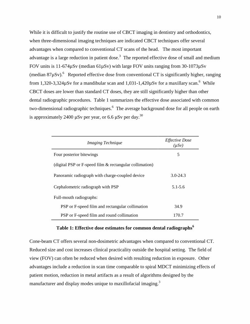
While it is difficult to justify the routine use of CBCT imaging in dentistry and orthodontics,

when three-dimensional imaging techniques are indicated CBCT techniques offer several

advantages when compared to conventional CT scans of the head. The most important

advantage is a large reduction in patient dose.3 The reported effective dose of small and medium

FOV units is 11-674µSv (median 61µSv) with large FOV units ranging from 30-1073µSv

(median 87µSv).6 Reported effective dose from conventional CT is significantly higher, ranging

from 1,320-3,324µSv for a mandibular scan and 1,031-1,420µSv for a maxillary scan.6 While

CBCT doses are lower than standard CT doses, they are still significantly higher than other

dental radiographic procedures. Table 1 summarizes the effective dose associated with common

two-dimensional radiographic techniques.6 The average background dose for all people on earth

is approximately 2400 µSv per year, or 6.6 µSv per day.30

Imaging Technique Effective Dose

(µSv)

Four posterior bitewings 5

(digital PSP or F-speed film & rectangular collimation)

Panoramic radiograph with charge-coupled device 3.0-24.3

Cephalometric radiograph with PSP 5.1-5.6

Full-mouth radiographs:

PSP or F-speed film and rectangular collimation 34.9

PSP or F-speed film and round collimation 170.7

Table 1: Effective dose estimates for common dental radiographs6

Cone-beam CT offers several non-dosimetric advantages when compared to conventional CT.

Reduced size and cost increases clinical practicality outside the hospital setting. The field of

view (FOV) can often be reduced when desired with resulting reduction in exposure. Other

advantages include a reduction in scan time comparable to spiral MDCT minimizing effects of

patient motion, reduction in metal artifacts as a result of algorithms designed by the

manufacturer and display modes unique to maxillofacial imaging.3

11

The Biologic Effects of Radiation

The biologic damage associated with radiation exposure is thought to be due to the direct action

of radiation on DNA as well as the indirect action of free radicals produced in water. Interaction

of radiation with water produces free oxygen radicals that interact with other molecules causing

damage to cell structures including DNA.31

In humans, the biologic effects of radiation can be categorized as stochastic (i.e. random) or

nonstochastic (i.e. non-random). Nonstochastic effects were previously referred to as acute

effects and in current terms ‘deterministic effects’.31

Deterministic effects are characterized by a

threshold below which effects are not observed. When the threshold is exceeded, the effects are

seen and the magnitude increases with increased dose. Such effects show a clear association

with radiation exposure.31

Examples include erythema, loss of hair, cataracts, nausea, vomiting

and depression of bone marrow cell division.31

Stochastic effects were previously referred to as “late effects” as they usually occur years after

exposure. Certain tissues are at higher risk for stochastic effects, in particular those composed

of cells with a high division rate, long dividing future and/or unspecialized type such as

progenitor cells found in bone marrow.31

Such effects may or may not present in a given

individual and are thus probabilistic in nature.31

The probability of stochastic effects increases

with radiation dose but not necessarily the magnitude of the effect. In contrast to nonstochastic

effects, a threshold may not exist and there lacks a clear association between exposure and effect.

Examples of stochastic effects include cancer and hereditary effects on the offspring of exposed

individuals.31

In oral and maxillofacial diagnostic imaging the primary concern is the risk for stochastic effects,

namely radiation induced cancer.2 This is because the doses given are all well below the

thresholds for deterministic effects. Recognizing the risk associated with radiation exposure,

prescription of dental and medical imaging must be done with diligence. Dosimetry studies

provide a means of estimating the biologic risk associated with radiation used in imaging or

therapy. Radiation dosimetry is the focus of this work.

12

Radiation Dosimetry

Interaction of radiation with matter results in a transfer of energy to the atoms constituting

tissue.31

Dosimetry is the determination of dose or the quantity of radiation exposure.2 Dose is

described in terms of the energy absorbed per unit mass at a site of interest. In clinical context,

dosimetry ultimately provides estimates of the biologic effects of radiation from which

appropriate therapeutic and diagnostic use can be determined. Several methods are used to

measure the quantitative effects of ionizing radiation with matter.

Exposure

When ionizing radiation interacts with matter ions are produced which have a net charge.

Counting the resulting ions formed in air is the simplest method for measuring the quantitative

effects of ionizing radiation. This can be accomplished by using oppositely charged surfaces to

attract and count the ions formed. The quantity exposure is a measure of radiation based on the

ability to produce ionization in air under standard temperature and pressure conditions. It

provides a measure of the radiation present in an environment and is useful in survey meter

measurements.31

Air kerma (‘kinetic energy released in matter’) is the SI unit of exposure and is

expressed in units of dose, Gray [Gy= 1 Joule/kg] replacing the traditional unit of Roentgen (R).2

Absorbed Dose

While exposure provides a measure of the radiation present in the environment, it is of greater

clinical importance to know the quantity of radiation actually absorbed by patients. The

‘absorbed dose’ describes the energy absorbed from any type of ionizing radiation per unit mass

of any type of matter.2,31

The SI unit for absorbed dose is also the Gy replacing the traditional unit of ‘rad’ (‘radiation

absorbed dose’) which is equal to 1cGy.2 The absorbed dose is thus determined by the following

equation:

13

Equivalent Dose

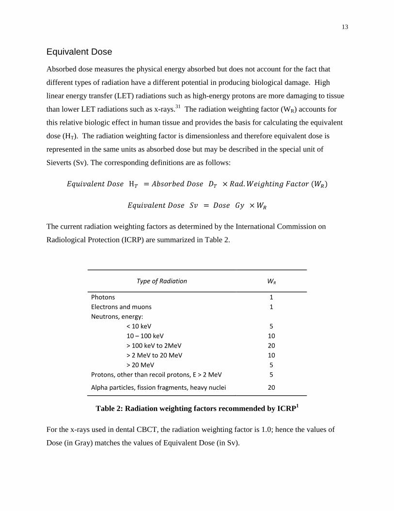
Absorbed dose measures the physical energy absorbed but does not account for the fact that

different types of radiation have a different potential in producing biological damage. High

linear energy transfer (LET) radiations such as high-energy protons are more damaging to tissue

than lower LET radiations such as x-rays.31

The radiation weighting factor (WR) accounts for

this relative biologic effect in human tissue and provides the basis for calculating the equivalent

dose (HT). The radiation weighting factor is dimensionless and therefore equivalent dose is

represented in the same units as absorbed dose but may be described in the special unit of

Sieverts (Sv). The corresponding definitions are as follows:

The current radiation weighting factors as determined by the International Commission on

Radiological Protection (ICRP) are summarized in Table 2.

Type of Radiation WR

Photons 1

Electrons and muons 1

Neutrons, energy:

< 10 keV 5

10 – 100 keV 10

> 100 keV to 2MeV 20

> 2 MeV to 20 MeV 10

> 20 MeV 5

Protons, other than recoil protons, E > 2 MeV 5

Alpha particles, fission fragments, heavy nuclei 20

Table 2: Radiation weighting factors recommended by ICRP1

For the x-rays used in dental CBCT, the radiation weighting factor is 1.0; hence the values of

Dose (in Gray) matches the values of Equivalent Dose (in Sv).

14

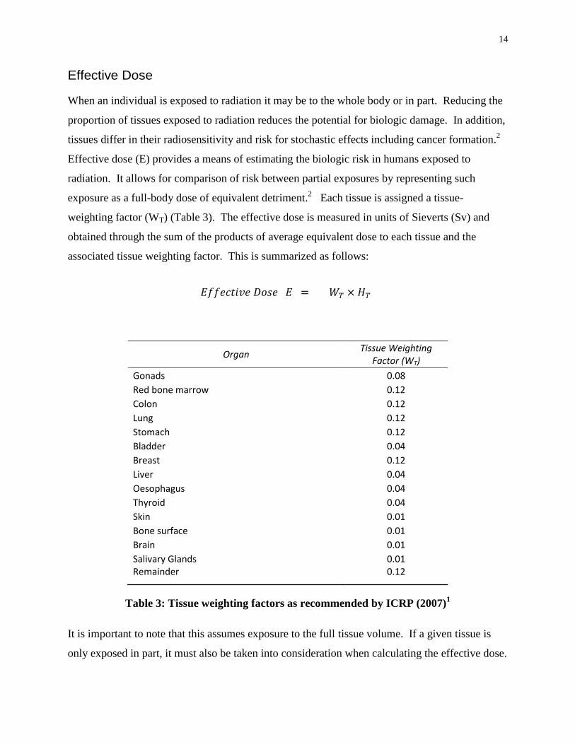
Effective Dose

When an individual is exposed to radiation it may be to the whole body or in part. Reducing the

proportion of tissues exposed to radiation reduces the potential for biologic damage. In addition,

tissues differ in their radiosensitivity and risk for stochastic effects including cancer formation.2

Effective dose (E) provides a means of estimating the biologic risk in humans exposed to

radiation. It allows for comparison of risk between partial exposures by representing such

exposure as a full-body dose of equivalent detriment.2 Each tissue is assigned a tissue-

weighting factor (WT) (Table 3). The effective dose is measured in units of Sieverts (Sv) and

obtained through the sum of the products of average equivalent dose to each tissue and the

associated tissue weighting factor. This is summarized as follows:

Organ Tissue Weighting

Factor (WT)

Gonads 0.08

Red bone marrow 0.12

Colon 0.12

Lung 0.12

Stomach 0.12

Bladder 0.04

Breast 0.12

Liver 0.04

Oesophagus 0.04

Thyroid 0.04

Skin 0.01

Bone surface 0.01

Brain 0.01

Salivary Glands 0.01 Remainder 0.12

Table 3: Tissue weighting factors as recommended by ICRP (2007)1

It is important to note that this assumes exposure to the full tissue volume. If a given tissue is

only exposed in part, it must also be taken into consideration when calculating the effective dose.

15

For example, in diagnostic radiology an image may only expose a fraction of the body’s skin.

The relative proportion of skin exposed is taken into consideration by multiplying the fraction

exposed by the skin's contribution to effective dose as follows:

Experimental Dosimetry Methods

There are several methods available for estimating the effective dose imparted by ionizing

radiation all of which rely on computations or measurements in patient-like ‘phantoms’ and

present with some limitations.32

The most common methods include organ dose, computed

tomography dose index by volume (CTDIvol), CT air kerma-length product (PKL,CT), Air kerma-

area product (PKA), Monte Carlo dose simulation programs, entrance surface skin dose and

energy imparted. Organ dose measurements or calculations using and Monte Carlo simulations

are common techniques employed in dental CBCT studies while CTDIvol measurement is most

common in conventional CT dosimetry studies and warrants discussion.

The computed tomography dose index by volume (CTDIvol) represents the mean absorbed dose

in the examination volume.32

A 100mm pencil ionization chamber is used to measure the kerma-

length product (PKL) at the centre and periphery of standardized cylindrical phantoms with

dimensions representing the head or body. The weighted CTDI (CTDIW) is the sum of one-third

of the value at the centre and two-thirds of the value at the periphery, corresponding to the

average dose in a slice, assuming abutted but non-overlapping slices. The CTDIvol is obtained by

dividing the CTDIW by the pitch used for examination to account for overlapping slices using

helical scanning.32

While this method has proven effective for single slice CT scanners with

slice thicknesses not exceeding 10mm, several studies have demonstrated limited applications to

thicker beam widths used in CBCT.33,34

As such, CTDIvol may present with limitations in

characterizing the dose associated with CBCT images.

Organ dose is based on estimates of the mean absorbed dose to different organs and tissues using

dosimeters placed locally within a human anthropomorphic phantom.32

These phantoms are

often composed of a natural human skeleton contained within a material radiologically

equivalent to human soft tissue. Accuracy in determining mean organ dose is limited given the

16

finite and limited number of dosimeters used. Effective dose is obtained using the mean tissue

doses and tissue weighting factors established by the ICRP.1 This method is the most

predominant in studies relating to CBCT dosimetry in dentistry.

Estimates of effective dose can also be obtained by mathematical models including Monte Carlo

simulations.32

This technique uses knowledge of exposure parameters and beam quality together

with a mathematical phantom of attenuation values to obtain an effective dose based on

simulation of individual particle interactions and trajectories.32

Dosimeters

Organ dose measurement is the most common dosimetry method found in dental CBCT studies.

The mean organ or tissue dose is determined by measuring the absorbed dose at a select number

of sites within a given organ or tissue. This is accomplished by use of dosimeters.

Thermoluminescent (TL) dosimeters are historically the most common used in dental CBCT

studies while newer optically stimulated luminescent (OSL) dosimeters are likely to become

more common as they have proven accurate while offering efficient readouts with the option of

being stored and reread at a later time.

Luminescence describes a process by which energy absorbed by a semiconductor or insulator

from ionizing radiation is subsequently released in the form of light (electromagnetic radiation)

upon exposure to heat (thermoluminescence, TLD) or light (optically stimulated luminescence,

OSL).35

This phenomenon is very useful in radiation dosimetry since the quantity of light

emitted is proportional to the radiation dose absorbed by the material.35

Many general models have been proposed to explain the mechanism of luminescence in select

materials, one of which is the electronic band model (EBM).35

The theory suggests the presence

of an energy band gap, or “forbidden band” separating two different energy bands, the valence

and conduction bands. Exposure to ionizing radiation results in excitation of electrons to the

conduction band with resulting holes in the valence band. These electrons and holes move

within the material until they recombine or are captured by localized intermediate energy levels

acting as traps. The trapped charges can be stimulated back to the conduction band with

subsequent de-excitation resulting in electron-hole recombination with resulting luminescence.

17

The intensity of luminescence is related to the trapped charge concentration and thus absorbed

dose. 36

For personal dosimetry, LiF:Mg,Ti (TLD-100) are the most common TL dosimeters used while

other suitable materials include LiF:Mg,Cu,P, CaSO4:Dy and ZrO2. 35

Another material

originally developed as a sensitive TLD material is Al2O3::C but its sensitivity to daylight instead

resulted in the research leading to OSL development.37

Additional materials that followed for

OSL include BeO, MgO, ABF fluorides, Ammonium salts and alkali halides.37

While

thermoluminescent dosimeters have been used successfully for many decades, use of OSL

dosimeters has become increasingly popular. Table 4 summarizes the characteristics of both TL

and OSL dosimeters.

TLD OSLD

Accuracy

High

(uncertainty ~3% for high

doses)35

High35

(uncertainty 0.7-3.2%) 36

Precision High

35

(reproducibility ~1.5%)38

High35

(reproducibility <1%)38

Dose Linearity Supralinear >10Gy 39

Supralinear >3Gy40

Reuse Reuseable35

Reuseable38

Energy Dependence Correction Factor Required41

Correction Factor Required41

Tissue Equivalence Tissue equivalent35

Nearly equivalent37

Size ~ 3x3x1mm 38

~ 7x7x0.5mm 38

Directional Dependence None35

3-4% 42

None38

Temperature Dependence Independent at ambient

temperature35

Independent

38

Fading Subject to fading35

Wait time of 8min

Slow fading day 17-38 38,43

Readout Time No instant readout

35

Technique sensitive

~ 8 min wait38

~1min to read

Table 4: Comparison of TLD and OSLD properties

18

CBCT Protocol Parameters

When a radiological examination is required an imaging protocol is established. A protocol is a

set of exposure parameters (kV, mAs, FOV) defined by the clinician and developed to produce

images of optimal quality while minimizing radiation burden to the patient.2 While standard

protocols are often pre-programmed by CBCT manufacturers, parameters may be modified by

the radiologist. Scan parameters usually include scanning volume (field of view), voxel size

(/resolution), the number of basis projections and exposure time. 2

Clinical guidelines suggest that radiation dose be optimized in accordance with the ALARA

principle. The principle states that dose should be restricted to as low as reasonably achievable.6

To accomplish this, the image should be restricted to a narrow field of view and produce image

quality sufficient to answer the clinical question being addressed. The quality of the image is

dependent on multiple parameters such as desired spatial and contrast resolution determined by

the clinician prior to exposure. An understanding of the effects of these parameters on both

image quality and dose is necessary to achieve an optimized protocol for each individual patient

and associated clinical question.

Field of View

Field of View (FOV) is established by collimating the primary x-ray beam, limiting x-radiation

to the region of interest thereby reducing effective dose by exposing only a subset of tissues and

organs.2 Maximum field of view differs between CBCT units on the market, with small FOV

machines beginning at 3x4x4mm (3D Accuitomo) and large FOV machines up to 20x20x20 cm

(NewTom 3G).44

Many units offer multiple FOV settings which may for example be suitable

for mandibular, maxillary or maxillofacial scans. Restricting the field of view to the region of

interest effectively reduces radiation dose and improves images quality by reducing scatter

radiation.2

Scan Time

A CBCT scan is composed of a series of basis radiographic image projections. In theory, a

perfect reconstruction is possible if an infinite number of two-dimensional projections are

obtained at an infinite number of angles. This of course in not practical and instead a finite

19

number of basis images is selected by adjusting the frame rate while the x-ray tube rotates.2

Increasing the number of basis projections increases image quality but patient exposure increases

proportionately.2

Exposure Time

For optimal image quality the radiographic projections measured at the detector must be neither

underexposed nor overexposed. This number of x-rays at the imaging detector is determined by

the number of x-rays produced, a product of milliamperage (mA) and exposure time (s).2 An

increase in milliampere-seconds (mAs) may improve image quality but at the expense of

increased patient radiation exposure. An optimum image protocol will establish an exposure

time for which image quality is diagnostic but patient exposure minimized.

CBCT Voxel Size

The voxel size varies between manufacturers with individual units often allowing user selection

of voxel size. A decrease in voxel size increases spatial resolution but results in increased

radiation exposure for a fixed noise level.2

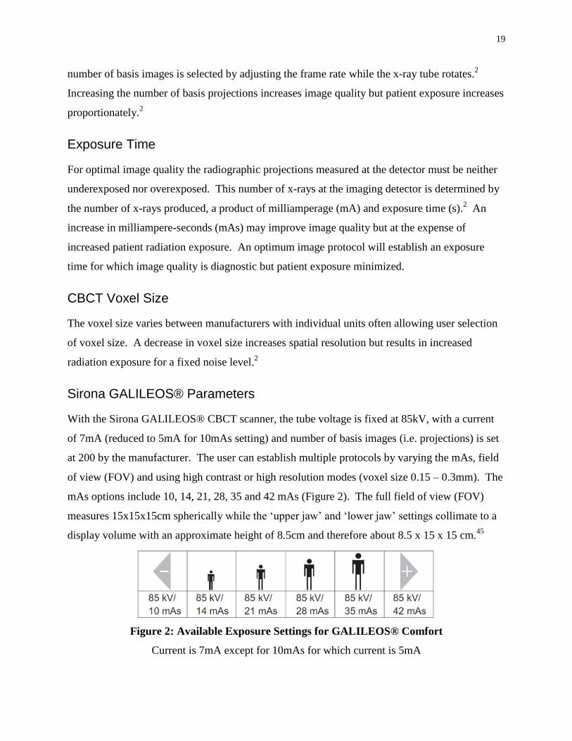
Sirona GALILEOS® Parameters

With the Sirona GALILEOS® CBCT scanner, the tube voltage is fixed at 85kV, with a current

of 7mA (reduced to 5mA for 10mAs setting) and number of basis images (i.e. projections) is set

at 200 by the manufacturer. The user can establish multiple protocols by varying the mAs, field

of view (FOV) and using high contrast or high resolution modes (voxel size 0.15 – 0.3mm). The

mAs options include 10, 14, 21, 28, 35 and 42 mAs (Figure 2). The full field of view (FOV)

measures 15x15x15cm spherically while the ‘upper jaw’ and ‘lower jaw’ settings collimate to a

display volume with an approximate height of 8.5cm and therefore about 8.5 x 15 x 15 cm.45

Figure 2: Available Exposure Settings for GALILEOS® Comfort

Current is 7mA except for 10mAs for which current is 5mA

20

A review of the current literature was conducted in order to identify studies investigating

dosimetry associated with the Sirona Galileos® CBCT scanner. A search was completed using

search terms ‘cone beam computed tomography’, ‘dosimetry’ and associated abbreviations and

truncated terms. Literature databases included PubMed, BIOSIS, EMBASE, CINAHL and

Dissertations and Theses. Studies matching initial search criteria were combined and reviewed

by title and abstract. Papers relevant to the research question were reviewed to determine the

inclusion of the Sirona GALILEOS® Comfort CBCT scanner. As of the writing of this thesis,

only 3 such papers were identified.

Ludlow and Ivanovic46

investigated the dosimetry associated with 8 dentoalveolar and

maxillofacial CBCT units, including the Sirona GALILEOS®, as well as a 64-slice MDCT unit.

Absorbed dose was measured for 24 select sites in the head and neck region using

thermoluminescent dosimeter (TLD) chips and a radiation analog dosimetry (RANDO®)

phantom. Effective dose was calculated to be 70µSv for default exposure (full FOV, 21mAs)

and 128µSv for maximum exposure (full FOV, 42mAs) based on 2007 ICRP1 tissue weighting

factors.

Pauwels et al47

determined the effective dose for a wide range of CBCT scanners and protocols

including the GALILEOS® Comfort.47

Absorbed dose was measured using between 147 – 152

TLD chips in anthropomorphic (ART) phantoms. The effective dose for the Sirona

GALILEOS® Comfort using a full FOV (15x15x15cm), 85kV and 28mAs was measured to be

84 µSv. Effective dose was also calculated based on 2007 ICRP1 tissue weighting factors. The

authors claim an improved accuracy as a result of an increased number and distribution of TL

dosimeters throughout the phantom.

Rottke et al48

evaluated the span of effective doses associated with ten different CBCT scanners

including the GALILEOS® Comfort. Absorbed dose was measured using TL dosimeters placed

in 24 sites in a RANDO® phantom following the protocol of Ludlow.46

The effective dose span

was established by measuring the doses for the lowest and highest exposure protocols. The

minimum exposure protocol using a full FOV, voxel size 0.15mm3 and current 7mA resulted in

an effective dose of 51µSv. Since the 10mAs exposure setting uses a reduced current of 5mA, it

is assumed the authors set the exposure at 14mAs. The maximum exposure protocol using a full

21

FOV, 0.3mm3 voxel size and 7mA (42mAs) current (/exposure) resulted in a measured effective

dose of 95µSv. Effective dose was again calculated based on 2007 ICRP1 tissue weighting

factors.

PURPOSE

While the number of dosimetry studies relating to CBCT units used in dentistry continues to

increase, few have reported findings associated with the Sirona GALILEOS® Comfort scanner

for its full range of operation. A review of the literature identified three such studies in which

only a restricted number of protocols were investigated. All protocols described were of full

maxillomandibular scans. With regard to exposure time, pooled data reveals effective dose

associated with mAs settings of 14, 21, 28 and 42. However, no single published study was

identified comparing the effective dose for a range of exposure and FOV settings.

The purpose of this thesis is to determine and compare the dosimetry associated with different

scanning protocols available with the Sirona GALILEOS® Comfort CBCT scanner. This

information should assist in determining the optimal scanning protocol for each patient when

combined with knowledge of respective effects on image quality.

22

MATERIALS AND METHODS

Absorbed dose was measured using optically stimulated luminescent (OSL) dosimeters placed

within a single, modified, male tissue-equivalent Alderson RANDO® phantom.

Dosimeters

Absorbed dose was measured at established sites using InLight® nanoDot

™ OSL dosimeters

(Landauer, Glenwood, Ill). OSL dosimeters offer a wide operating energy range, efficient

readings and reanalysis capabilities with minimal angular and energy dependence.38

In total, 27 OSL dosimeters were used throughout the study. All dosimeters were calibrated

using a Therapax HF150 superficial radiation therapy x-ray unit (Pantak, East Haven, CT) with a

1.1mm Al +0.3mm Cu filter. This filter allowed for production of a beam quality similar to that

of the GALILEOS® Comfort confirmed by measurement of the respective Half Value Layer

(HVL). The Therapax unit allows user control over kVp, mA, exposure time and source to

object distance. Groups of OSL dosimeters not exceeding the beam field were positioned flat on

a Polymethyl methacrylate (PMMA) block 140mm in height (Figure 3). This platform

approximated the dimensions of the human phantom to account for similar amounts of

backscatter radiation. The OSL dosimeters were exposed at fixed dose intervals and read until

the cumulative count exceeded the maximum count of the OSL dosimeters used for phantom

protocols. Each OSLD was read using a microstar OSLD reader (Landauer, Glenwood, Ill),

taken as the average of three repeated readings. Each exposure was measured under identical

conditions using a Farmer Chamber and Capintec 192 Digital Exposure Meter (Capintec,

Ramsay NJ) with calibration traceable to national standards. Respective calibration curves were

established to characterize each individual OSLD and obtain corrected dose from each OSLD

reading. Appropriate adjustments were made for room temperature and pressure.

23

Figure 3: Therapax HF 150

1.1mm Al + 0.3mm Cu filter, Farmer Chamber & PMMA background

Phantom

The head and neck segment of the RANDO® phantom consists of 10 sections, each with

predrilled holes designed to accommodate thermoluminescent dosimeters (TLDs). In order to

place OSL dosimeters, five PMMA templates (Figure 4) 2.15mm thick were fabricated and

placed superior to sections three, four, six, seven and nine (Figure 5). In diagnostic radiology,

PMMA is the most tissue equivalent material used.49

Square holes were placed in each template

large enough to accommodate OSL dosimeters at anatomical landmarks without allowing

movement.

24

Figure 4: PMMA template for OSLD placement

Figure 5: RANDO® phantom with PMMA templates in place

25

Anatomic Landmarks

Twenty six sites were measured corresponding to the 24 anatomical positions described by

Ludlow (Table 5).50

Two sites each were established for the left and right mandibular body.

Due to difficulty approximating the centre of the body, one site was positioned superior to and

another inferior to the mandibular body with the average absorbed dose representing that of the

mandibular body. An additional OSLD was used to measure background radiation and was

present beside the operator during acquisition and remained with the other dosimeters during

transport.

Anatomic Location OSLD

Number OSLD ID

Calvarium anterior 1 34151D Calvarium left 2 42477T Calvarium posterior 3 42098X Midbrain 4 44986I Pituitary 5 46848I Right orbit 6 29436W Left orbit 7 48908I Right lens of eye 8 41606Z Left Lens of eye 9 46757L Right cheek 10 409410 Right parotid 11 27592Y Left parotid 12 37841X Right ramus 13 26177Z Left ramus 14 32758P Centre cervical spine 15 31835W Left back of neck 16 44131D Right mandible body upper 17 45032C Right mandible body lower 18 35299O Left mandible body upper 19 32817T Left mandible body lower 20 48629K Right submandibular gland 21 31657U Left submandibular gland 22 32871Z Centre sublingual gland 23 28791V Midline thyroid 24 46970B Thyroid surface - left 25 294126 Esophagus 26 35015A Background 27 321268

Table 5: Anatomic sites for dosimeter placement

26

Each phantom is constructed of a natural human skeleton cast inside a standard mold composed

of a material radiologically simulating soft tissue. Initial images of the phantom revealed

discrepancies between soft tissue contours of the head and neck and the underlying skeleton

(Figure 6). Dosimeter sites for skeletal and internal soft tissue landmarks were established in

relation to the skeleton while surface landmarks were established with respect to soft tissue sites

on the RANDO® phantom. Surface landmarks were marked with tape over which OSL

dosimeters were centred for each protocol.

Figure 6: Relationship of hard and soft tissue in RANDO® phantom

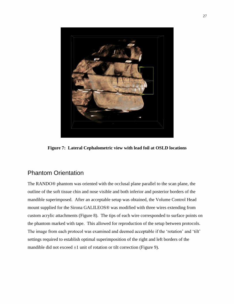
With the PMMA templates in place, lead foil from intraoral radiograph packets was placed in

each internal OSLD location and a 3D scan completed. The reconstructed image was examined

to confirm acceptable location of each internal landmark (Figure 7).

27

Figure 7: Lateral Cephalometric view with lead foil at OSLD locations

Phantom Orientation

The RANDO® phantom was oriented with the occlusal plane parallel to the scan plane, the

outline of the soft tissue chin and nose visible and both inferior and posterior borders of the

mandible superimposed. After an acceptable setup was obtained, the Volume Control Head

mount supplied for the Sirona GALILEOS® was modified with three wires extending from

custom acrylic attachments (Figure 8). The tips of each wire corresponded to surface points on

the phantom marked with tape. This allowed for reproduction of the setup between protocols.

The image from each protocol was examined and deemed acceptable if the ‘rotation’ and ‘tilt’

settings required to establish optimal superimposition of the right and left borders of the

mandible did not exceed ±1 unit of rotation or tilt correction (Figure 9).

28

Figure 8: Modified mount for setup reproduction

Figure 9: 'Tilt' and 'Rotation', confirming setup reproduced

29

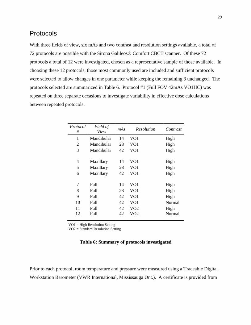
Protocols

With three fields of view, six mAs and two contrast and resolution settings available, a total of

72 protocols are possible with the Sirona Galileos® Comfort CBCT scanner. Of these 72

protocols a total of 12 were investigated, chosen as a representative sample of those available. In

choosing these 12 protocols, those most commonly used are included and sufficient protocols

were selected to allow changes in one parameter while keeping the remaining 3 unchanged. The

protocols selected are summarized in Table 6. Protocol #1 (Full FOV 42mAs VO1HC) was

repeated on three separate occasions to investigate variability in effective dose calculations

between repeated protocols.

Protocol

#

Field of

View mAs Resolution Contrast

1 Mandibular 14 VO1 High



4 Maxillary 14 VO1 High



7 Full 14 VO1 High

8 Full 28 VO1 High

9 Full 42 VO1 High

10 Full 42 VO1 Normal

11 Full 42 VO2 High

12 Full 42 VO2 Normal

Table 6: Summary of protocols investigated

Prior to each protocol, room temperature and pressure were measured using a Traceable Digital

Workstation Barometer (VWR International, Mississauga Ont.). A certificate is provided from

VO1 = High Resolution Setting

VO2 = Standard Resolution Setting

30

an ISO 17025 calibration laboratory accredited by A2LA to indicate instrument traceability to

standards provided by the National Institute of Standards and Technology.

Each scanning protocol was repeated three times prior to removing the OSL dosimeters from the

phantom to minimize the contribution of noise to absorbed dose. Absorbed dose was thus

obtained by dividing the dose measured by three. At least 15 minutes was ensured between

scanning and reading the dosimeters as suggested by the manufacturer. This allows low-level,

non-dosimetric electron traps to stabilize.38

The dosimeters were read using a microstar OSLD reader (Landauer, Glenwwod, Ill) taking the

mean value of three subsequent readings. They were annealed using a high intensity light source

(Figure 10) after no more than three subsequent protocols to minimize the increase in

measurement uncertainty associated with dose accumulation.

Figure 10: High intensity light source to anneal OSL dosimeters

Dosimeter counts were entered into a spreadsheet and absorbed dose determined by means of

applying individual calibration curves. Effective dose was calculated using the mean absorbed

dose to the individual tissues and organs, applying the corresponding 2007 ICRP1 tissue

weighting factors and correcting for the fractional volume of tissue irradiated. The fraction of

tissue irradiated was determined by following that outlined by Ludlow and Ivanovic.46

A

correction factor of 2.76 was applied for bone surface dose relative to bone marrow dose based

31

on the ratio of mass energy absorption coefficients for bone and muscle. The ratio is energy

dependent and was chosen for a kVp of 85 and Half Value Layer (HVL) of 7mm of Aluminum.51

However a correction for enhanced backscatter from bone was not applied.52

Table 7 lists the

dosimeters used to sample each tissue and summarizes the respective fraction of tissue irradiated

and tissue weighting factors. For those tissues located outside of the head and neck, absorbed

dose was assumed to be negligible.

Tissue/Organ ID of OSLDs Used to

Sample Tissue

Fraction of

Tissue

Irradiated (%)

Tissue Weighting Factor

(WT)

Red bone marrow 16.5 0.12

Mandible 13, 14, 17-20 1.3

Calvaria 1, 2, 3 11.8

Cervical Spine 15 3.4

Oesophagus 26 10 0.04

Thyroid 24, 25 100 0.04

Skin 8, 9, 10, 16 5 0.01

Bone surface 16.5 0.01

Mandible 13, 14, 17-20 1.3

Calvaria 1, 2, 3 11.8

Cervical Spine 15 3.4

Brain 4,5 100 0.01

Salivary Glands 11, 17-23, 12, 21, 22, 23 100 0.01

Remainder 0.12

Lymphatic nodes 11-15, 17-24, 26 6

Muscle 11-15, 17-24, 26 6

Extrathoracic Airway 6, 7, 11-15, 17-24, 26 100

Oral mucosa 11-14, 17-23 100

Gonads 0 0.08

Colon 0 0.12

Lung 0 0.12

Stomach 0 0.12

Bladder 0 0.04

Breast 0 0.12

Liver 0 0.04

Table 7: Percentage tissue irradiated, tissue weighting factor and OSLD sample for each

tissue/organ

32

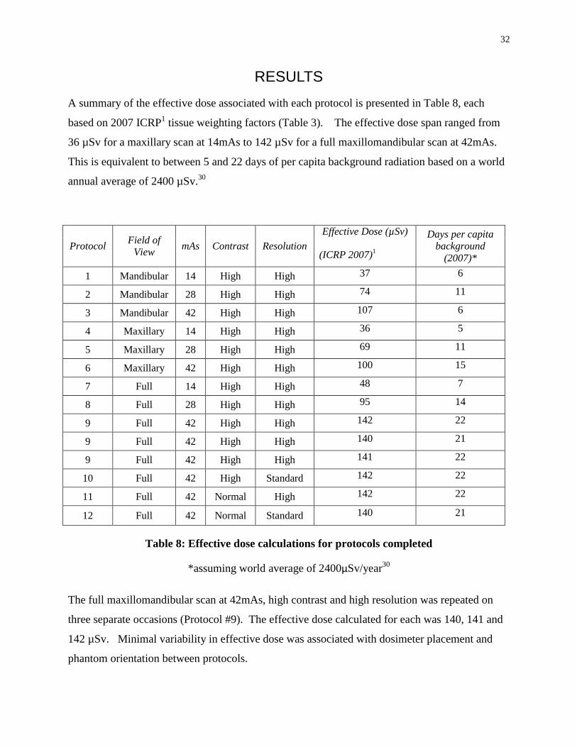
RESULTS

A summary of the effective dose associated with each protocol is presented in Table 8, each

based on 2007 ICRP1 tissue weighting factors (Table 3). The effective dose span ranged from

36 µSv for a maxillary scan at 14mAs to 142 µSv for a full maxillomandibular scan at 42mAs.

This is equivalent to between 5 and 22 days of per capita background radiation based on a world

annual average of 2400 µSv.30

Protocol Field of

View mAs Contrast Resolution

Effective Dose (µSv)

(ICRP 2007)1

Days per capita

background

(2007)*

1 Mandibular 14 High High 37 6



4 Maxillary 14 High High 36 5



7 Full 14 High High 48 7





10 Full 42 High Standard 142 22

11 Full 42 Normal High 142 22

12 Full 42 Normal Standard 140 21

Table 8: Effective dose calculations for protocols completed

*assuming world average of 2400µSv/year30

The full maxillomandibular scan at 42mAs, high contrast and high resolution was repeated on

three separate occasions (Protocol #9). The effective dose calculated for each was 140, 141 and

142 µSv. Minimal variability in effective dose was associated with dosimeter placement and

phantom orientation between protocols.

33

Collimating for a maxillary or mandibular scan resulted in a reduced effective dose relative to a

full maxillomandibular scan. Table 9 shows the effective dose for both maxillary and

mandibular scans as a percentage of a full scan for each mAs investigated. All scans were high

resolution and high contrast. The effective dose associated with a full maxillomandibular scan is

reduced on average by 28% when collimated for a maxillary scan and 23% when collimated for a

mandibular scan. This exceeds the 15% approximation reported by Sirona.45

Field of

View 14mAs 28mAs 42mAs Mean

Maxillary 74% 73% 70% 72%

Mandibular 78% 78% 76% 77%

Table 9: Effective dose of collimated scans

as a percentage of full maxillomandibular scan dose by mAs

Figure 11 depicts the changes in effective dose with increasing mAs for maxillary, mandibular

and full fields of view. All scans were at high resolution and contrast. Both maxillary and

mandibular scans show a similar effective dose reduction relative to a full scan throughout the

range of mAs settings. This difference increases in magnitude with increasing mAs. An

increase in mAs results in a linear and proportional increase in effective dose for all fields of

view.

Figure 11: Effective Dose vs mAs

0

20

40

60

80

100

120

140

160

0 10 20 30 40 50

Effe

ctiv

e D

ose

(µ

Sv)

mAs

Dose (µSv) vs mAs

Full Scan

Maxillary Scan

MandibularScan

34

The mean equivalent dose to individual organs and tissues is summarized in Table 10. Table 11

compares the equivalent doses for maxillary scans as a percentage of the equivalent doses for

mandibular scans, taking the mean of 14, 28 and 42 mAs percentages. While the effective

doses for maxillary and mandibular scans are similar, the distribution of equivalent doses to the

tissues differs. For a maxillary scan, the equivalent dose to the brain is on average 298% of that

for a mandibular scan and similarly 146% for skin and 140% for bone marrow.

Protocol Bone

Marrow

Thyroi

d

Esophagu

s Skin

Bone

Surface

Salivary

Glands Brain

Lymphati

c Nodes

Extrathoraci

c Region Muscle

Oral

Mucosa

Remainder Tissues

Full 14mAs VO1HC 73 112 4 36 202 1104 447 889 856 889 1020

Full 28mAs VO1HC 139 233 19 67 382 2225 776 1793 1719 1793 2042

Full 42mAs VO1HC #1 208 335 32 98 573 3372 1150 2683 2582 2683 3058

Full 42mAs VO1HC #2 206 351 30 100 568 3296 1108 2638 2536 2638 3005

Full 42mAs VO1HC #3 211 327 33 102 583 3328 1144 2665 2557 2665 3025

Full 42mAs VO1NC 201 359 31 102 555 3418 1109 2659 2559 2659 3028

Full 42mAs VO2HC 211 322 30 105 582 3363 1157 2686 2584 2686 3065

Full 42mAs VO2 NC 206 326 29 105 567 3320 1123 2646 2546 2646 3021

Max 14mAs VO1HC 69 45 0 29 189 707 442 632 630 632 710

Max 28mAs VO1HC 131 97 5 62 361 1399 785 1242 1239 1242 1383

Max 42mAs VO1HC 185 145 10 93 511 2016 1090 1793 1794 1793 1989

Mand 14mAs VO1HC 51 90 3 25 139 956 196 782 701 782 909

Mand 28mAs VO1HC 94 204 13 41 260 1966 257 1588 1413 1588 1830

Mand 42mAs VO1HC 129 299 24 56 355 2917 301 2327 2068 2327 2687

Table 10: Equivalent dose (µSv) to tissues/organs

Bone Marrow Thyroid Esophagus Skin Bone

Surface

Salivary

Glands Brain

Lymphatic

Nodes

Extrathoracic

Region Muscle

Oral

Mucosa

140% 49% 27% 146% 140% 71% 298% 79% 88% 79% 76%

Table 11: Equivalent doses for maxillary scan as a percentage of equivalent doses for

mandibular scan (taken as mean of percentages for 14, 28 and 42 mAs)

VO1 = High Resolution

VO2 = Standard Resolution

HC = High Contrast

NC = Normal Contrast

35

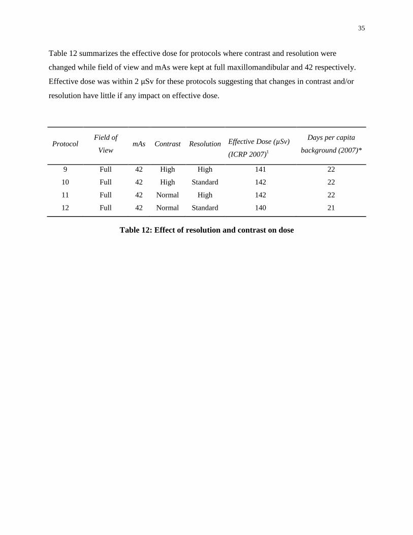
Table 12 summarizes the effective dose for protocols where contrast and resolution were

changed while field of view and mAs were kept at full maxillomandibular and 42 respectively.

Effective dose was within 2 µSv for these protocols suggesting that changes in contrast and/or

resolution have little if any impact on effective dose.

Protocol Field of

View mAs Contrast Resolution Effective Dose (µSv)

(ICRP 2007)1

Days per capita

background (2007)*


10 Full 42 High Standard 142 22

11 Full 42 Normal High 142 22

12 Full 42 Normal Standard 140 21

Table 12: Effect of resolution and contrast on dose

36

DISCUSSION

The mean effective dose calculated for the maximum exposure (maxillomandibular scan,

42mAs, high contrast, high resolution) was 141 µSv. This compares with previous findings,

Ludlow and Ivanovic46

who reported 128 µSv and Rottke et al48

who reported 95 µSv. The

effective dose calculated for a maxillomandibular scan at 28mAs (high contrast, high resolution)

was 95 µSv compared to 84µSv reported by Pauwels et al.47

All reports are based on 2007

ICRP1 tissue weighting factors. It is important when making comparisons between studies that

the same weighting factors are used. In general, effective dose based on 1990 ICRP tissue

weighting factors is significantly reduced relative to 2007 due to the increased weighting factors

for salivary gland tissue and brain introduced in 2007.

During this study, calibration curves for each OSLD were initially established by two methods.

The method used in this study simulated conditions of surface dosimeters (‘free in air’ with

PMMA background) while the other simulated conditions of dosimeters placed internally by

placing them under 5cm of PMMA. A 5cm PMMA barrier was chosen when it was estimated

that the beam was attenuated by an average of 5cm of phantom tissue prior to reaching the

internal dosimeters. The ‘free in air’ method with a PMMA background was chosen for the

definitive calibration method in order to minimize the risk of underestimating effective dose.

Preliminary calculations using ‘in plastic’ calibration curves determined an effective dose of 102

µSv for a full scan at 42 mAs as compared to the definitive calculation of 141 µSv using ‘in air’

calibration.

The discrepancy between effective dose calculations based on ‘free in air’ and ‘in plastic

(PMMA)’ calibration curves reveals the importance of the calibration process in obtaining

accurate effective dose estimates. Ludlow and Ivanovic46

reported the use of

thermoluminescent dosimeters that were precalibrated and analyzed by the supplier Lindauer

(Glenwood, IL). It is unclear under what conditions respective calibration curves were

established. Pauwels et al47

reported the use of two types of TLDs, one type calibrated free in

air, the other by calibrating internal calibration dosimeters for each experiment. Rottke et al48

calibrated each TLD to obtain individual calibration factors. Those with calibration factors

outside two standard deviations were excluded while an average calibration factor was used for

37

effective dose calculation. There is no mention whether calibration was completed ‘free in air’

or under different conditions.

An additional property that is significant when using dosimeters is their angular dependence. It

is possible that the orientation of a dosimeter to the primary beam affects the dose measured.

Thermoluminescent dosimeters are directionally independent.35

There is conflicting evidence

with regard to the angular dependence of OSL dosimeters with a study by Jursinic38

finding no

angular dependence when exposed to 50 cGy of 6 MV x-rays while Kerns et al42

report a 3-4%

variation in OSLD response with variation in dosimeter orientation relative to a 6 and 18MV

photon beam. It may be ideal to calibrate the dosimeters at their defined positions in the

RANDO® phantom to circumvent the issues of orientation and ‘in air’ versus ‘in plastic’

calibration. However, there is no means to acquire standardized reference dose measurements at

these sites using an ion chamber.

This study aimed to identify the effect of each parameter on effective dose. A reproducible set-

up is of great importance such that comparisons can be made between different protocols. Once

an acceptable position of the phantom was obtained, a modified Volume Control Head Mount

was used to reproduce positioning based on three surface points. After each protocol the ‘tilt’

and ‘rotation’ settings were modified to obtain optimal superimposition of the posterior and

inferior borders of the mandible. A set-up was deemed to be adequately reproduced if these

settings did not deviate more than ±1 tilt or rotation correction unit. This range was established

arbitrarily prior to the study. It is unclear if the tilt and rotations settings correspond to a given

number of degrees but it was observed that modifying the tilt or rotation ±1 corresponded to

relatively little movement of the image. Using the modified head mount proved successful with

every protocol adequately reproducing the original. To investigate the reproducibility of

effective dose measurement, a maxillomandibular protocol with maximum exposure (42mAs,

high contrast, high resolution) was repeated on three separate occasions. The effective dose was

very similar measuring 140, 141 and 142 µSv.

Thermoluminescent dosimeters have been used with success for many decades and account for

the majority of dosimeters used in organ dose phantom studies in dentistry. As a result, most

phantoms in use are prepared with predrilled holes to accommodate TL dosimeters. These are

38

often cylindrical and smaller in size than the InLight® nanoDot

™ OSL dosimeter (Landauer,

Glenwood, Ill) used in this study. Optically stimulated luminescent dosimeters were chosen for

use in this study as they were already in established use in our associated clinical cancer therapy

facility. They offer acceptable accuracy and precision, less dependence on technique and

operator and less concerns with respect to signal fading between radiation exposure and readout.

A review of the literature revealed only one dental CBCT dosimetry study using OSL

dosimeters. Al Najjar et al53

compared the adult and child radiation equivalent dose from two

dental CBCT units. They used OSL dosimeters of unspecified type and head phantoms

manufactured specifically to accommodate OSL dosimeters. Comparing results between studies

can be difficult due to differences in phantom and dosimeters used. In this study, a RANDO®

phantom previously prepared for use with TL dosimeters was modified to accommodate OSL

dosimeters using five 2.15mm thick PMMA templates designed to fit between the phantom

sections. This effectively increases the dimensions of the phantom by approximately 11mm and

could therefore affect absorbed doses by displacing OSL dosimeters located more superiorly and

inferiorly further from the primary beam. While PMMA is commonly used in dosimetry studies

due to its tissue equivalent properties, its attenuation value may differ from that of the RANDO®

phantom.

An advantage of TL dosimeters for the phantom used is the potential to place the dosimeters

anywhere within the phantom. With the modified phantom, OSL dosimeter placement was

restricted to the PMMA templates between phantom sections. Initial images revealed that the

skull was not well related to the soft tissue contours with the hard tissue chin displaced quite

superiorly. Each phantom is composed of a natural human skull cast inside a standard soft tissue

mold and thus each phantom is unique. Variations in the natural skulls between phantoms could

affect the appropriate section for dosimeter placement and the relationship of tissues and

structures to the primary beam. In this study we chose to place internal dosimeters according to

hard tissue references and external dosimeters according to soft tissue landmarks. Accuracy in

the spatial relationship between internal and external dosimeters was limited by the phantom

anatomy. The phantom was oriented with the goal of maximizing hard tissue structures and soft

tissue contours of interest. It is possible that superior and inferior structures were further

displaced from the primary beam due to the anatomy of the phantom. An image obtained with

lead foil in place of dosimeters revealed reasonable approximation to the tissues and structures of

39

interest. While the phantom anatomy and need for modification to accommodate OSL

dosimeters does present some limitations, comparisons between protocols within the study

remain valid.

Optically stimulated luminescent dosimeters were selected for this study. They provide a more

efficient and less technique sensitive reading than TL dosimeters and not subject to the same

degree of fading. They have good accuracy and precision and are suitable for dosimetry studies.

A logistical advantage of OSL dosimeters is the potential for incremental use where, unlike

TLDs, minimal charge is lost during analysis (0.04-0.25%).54

The manufacturer discourages

continued incremental use since a supralinear dose response is noted when accumulated dose

exceeds 300cGy and the uncertainty of measurements can increase from 2% to as much as 4%.

A 100 cGy dose corresponds to an approximate signal of 130 000 counts with the OSL dosimeter

used.38

For logistical reasons, OSL dosimeters were used for incremental measures with up to

three protocols measured prior to annealing for re-use. The accumulated signal did not exceed

100 000 counts and therefore well within the range of a linear dose response.

One comparison of interest is the effect of resolution and contrast settings on effective dose.

With the Sirona GALILEOS® Comfort CBCT scanner, the user has the options of high or

standard contrast and resolution settings. A full maxillomandibular scan was completed at

42mAs for all 4 resolution and contrast combinations. There was no significant difference in

effective dose between the four protocols. The manufacturer reports that both high and standard

resolution options produce a data volume set with 512 x 512 x 512 voxels. The high-resolution

secondary reconstruction can be generated by the software only if the high-resolution setting is

selected. Specific information regarding the difference between high and standard settings for

resolution and contrast proved difficult to obtain. Limited information available suggested that

pixel binning occurs if the high-resolution setting is selected thus transferring data with a voxel

size of 0.3mm but maintaining the capability of reconstructing an image with 0.15mm voxel size

post acquisition. The standard resolution does not maintain this capability but may as a result

allow for faster data transfer. These results suggest that there is little benefit in selecting the

standard resolution setting and contrast settings should be chosen based on optimizing the tissues

of interest. It is likely the same projection set is acquired regardless of the contrast and

resolution software settings selected prior to image acquisition.

40

An important clinical decision when obtaining a CBCT image is selecting the field of view as

additional information can be obtained with a larger field of view but at the expense of increased

patient exposure. This decision will be based on potential structures of clinical interest and the

associated dose incurred when acquiring the image. The results of this study suggest that

collimating to a maxillary or mandibular scan results in a reduction in effective dose of

approximately 28% and 23% respectively, this exceeds the approximate 15% reported by the

manufacturer. It should be noted that no modifications were made to the percentage of tissue

irradiated when calculating the effective dose for partial scans. It could be argued that respective

reductions should be made which could result in additional reduction in effective dose when

partial scans are selected. A review of previous literature revealed only one study adjusting

fraction of tissue irradiated for partial scans with adjustments based on the opinion of the local

radiologist.55

No modification to the fraction of tissue irradiated was elected as it was observed

that all dosimeters registered a significant dose for partial scans. This ‘conservative’ approach

reduces the risk of under reporting the effective dose but may as a result neglect to report the full

benefit in dose reduction when selecting a collimated protocol. Based on these findings it is

apparent a moderate reduction in effective dose is realized when selecting a partial scan.

However, if structures present on a full scan are omitted by collimation and may be of interest in

the future, consideration towards a full scan is justified as the cumulative dose of two separate

partial scans is likely to exceed that of a full scan.

The primary aim of this study was to investigate the impact different parameters had on effective

dose. Ideally each of the 72 potential protocols would be investigated individually. This would

allow more robust statistical analysis of linearity when comparing effective dose with changes in

mAs. In addition, changes in contrast and resolution settings were investigated only for full

maxillomandibular scans at 42mAs. While a similar data acquisition process is likely for the

remaining field of views and mAs settings, this cannot not be concluded with certainty.

Effective dose is important when determining the optimum scanning protocol for an individual

patient and clinical question. The information provided by this study is useful in understanding

the relative effects each parameter has on effective dose. It is important to understand that

establishing an optimum protocol must also consider image quality. Collimation reduces the

amount of structures visible on the image while changes in mAs, contrast and resolution can and

41

often do impact the image quality. Such changes may or may not impact diagnosis. Future study

of the impact of the same parameters on image quality (e.g. standard tests of spatial and contrast

resolution) would provide equally important information in determining optimum scanning

protocols using the Sirona Galileos® CBCT scanner.

42

SUMMARY

The aim of this study was to measure and compare the effective dose associated with a sample of

protocols available using the Sirona GALILEOS® Comfort CBCT scanner. With this unit the

tube voltage and number of basis projections are set by the manufacturer to 85kVp and 200

respectively. The user can establish a protocol by selecting between mAs, contrast, resolution

and collimation settings. This study investigated 12 protocols with modifications to all four

parameters.

Results revealed a dose span of 48 µSv to 142 µSv for a full maxillomandibular scan, relatively

low when compared to conventional CT units but significantly higher than panoramic and lateral

cephalometric exposures. Effective dose varied linearly with mAs while contrast and

resolutions settings had little impact on effective dose for this scanner. A moderate reduction in

effective dose can be realized when collimating for a partial scan.

Cone beam computed tomography can provide significant diagnostic value when prescribed

appropriately. Further evidence is needed to clarify when the clinical benefit justifies the burden

of additional radiation exposure. When a CBCT image is justified, the results of this study will

assist the clinician in determining the optimum protocol for each patient when considered in the

context of diagnostic or treatment planning applications.

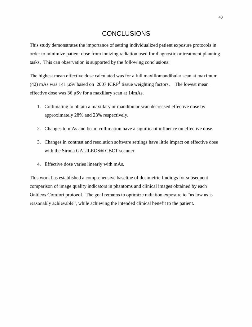
43

CONCLUSIONS

This study demonstrates the importance of setting individualized patient exposure protocols in

order to minimize patient dose from ionizing radiation used for diagnostic or treatment planning

tasks. This can observation is supported by the following conclusions:

The highest mean effective dose calculated was for a full maxillomandibular scan at maximum

(42) mAs was 141 µSv based on 2007 ICRP1 tissue weighting factors. The lowest mean

effective dose was 36 µSv for a maxillary scan at 14mAs.

1. Collimating to obtain a maxillary or mandibular scan decreased effective dose by

approximately 28% and 23% respectively.

2. Changes to mAs and beam collimation have a significant influence on effective dose.

3. Changes in contrast and resolution software settings have little impact on effective dose

with the Sirona GALILEOS® CBCT scanner.

4. Effective dose varies linearly with mAs.

This work has established a comprehensive baseline of dosimetric findings for subsequent

comparison of image quality indicators in phantoms and clinical images obtained by each

Galileos Comfort protocol. The goal remains to optimize radiation exposure to “as low as is

reasonably achievable”, while achieving the intended clinical benefit to the patient.

44

REFERENCES

1. ICRP. The 2007 recommendations of the international commission on radiological protection.

ICRP publication 103. Ann ICRP. 2007;37:2-4.

2. White SC, Pharoah MJ. Oral radiology :Principles and interpretation. 6th ed. St. Louis, Mo.:

Mosby/Elsevier; 2009:641.

3. Scarfe WC, Farman AG, Sukovic P. Clinical applications of cone-beam computed tomography

in dental practice. J Can Dent Assoc. 2006;72(1):75-80.

4. ICRP. The optimisation of radiological protection: Broadening the process. ICRP publication

101. approved by the commission in september 2005. Ann ICRP. 2006;36(3):65, 71-104.

5. National Council on Radiation Protection and Measurements. Radiation protection in dentistry

:Recommendations of the national council on radiation protection and measurements (report no.

145). Vol 145. Bethesda, MD: National Council on Radiation Protection and Measurements;

2003:191.

6. American Dental Association Council on Scientific Affairs. The use of cone-beam computed

tomography in dentistry: An advisory statement from the american dental association council on

scientific affairs. J Am Dent Assoc. 2012;143(8):899-902.

7. Iannucci JM, Iannucci JM. Dental radiography :Principles and techniques. 4th; 4th ed. St.

Louis, Mo.; St. Louis, Mo.: Elsevier/Saunders; Elsevier/Saunders:466; 466.

8. Kantor ML. Dental digital radiography: More than a fad, less than a revolution. J Am Dent

Assoc. 2005;136(10):1358, 1360, 1362.

45

9. Mouyen F, Benz C, Sonnabend E, Lodter JP. Presentation and physical evaluation of

RadioVisioGraphy. Oral Surgery, Oral Medicine, Oral Pathology. 1989;68(2):238-242.

10. Crawford PR. 100 years of radiology: Those early years. J Can Dent Assoc.

1995;61(11):951-954.

11. Finlay LM. Craniometry and cephalometry: A history prior to the advent of radiography.

Angle Orthod. 1980;50(4):312-321. doi: 2.

12. Pacini AJ. Roentgen ray anthropometry of the skull. J Radiol. 1922(3):230-238, 322-331,

418-426.

13. Allen WI. Historical aspects of roentgenographic cephalometry. Am J Orthod.

1963;49(6):451-459.

14. Seynaeve PC, Broos JI. The history of tomography. J Belge Radiol. 1995;78(5):284-288.

15. Hallikainen D. History of panoramic radiography. Acta Radiol. 1996;37(3 Pt 2):441-445.

16. Frank ZA. Panoramic x-ray apparatus. . 1922(1408559).

http://www.freepatentsonline.com/1408559.html.

17. PAATERO YV. Radiography of the temporo-mandibular joint; a new method. Ann Chir

Gynaecol Fenn. 1953;42(4):259-264.

18. PAATERO YV. Geometrical study on possibilities of making double eccentric

pantomograms with a single exposure. Suom Hammaslaak Toim. 1954;50(Suppl. 2):36-43.

19. PAATERO YV. Pantomography in theory and use. Acta Radiol. 1954;41(4):321-335.

http://www.freepatentsonline.com/1408559.html

46

20. PAATERO YV. Pantomography of spherical layers. Acta Radiol. 1957;48(3):181-187.

21. Dove SB, McDavid WD, Welander U, Tronje G. Preliminary evaluation of a digital system

for rotational panoramic radiography. Oral Surg Oral Med Oral Pathol. 1992;73(5):623-632.

22. McDavid WD, Dove SB, Welander U, Tronje G. Electronic system for digital acquisition of

rotational panoramic radiographs. Oral Surg Oral Med Oral Pathol. 1991;71(4):499-502.

23. Kashima I, Kanno M, Higashi T, Takano M. Computed panoramic tomography with

scanning laser-stimulated luminescence. Oral Surg Oral Med Oral Pathol. 1985;60(4):448-453.

24. Kalender W. Computed tomography :Fundamentals, system technology, image quality,

applications. 3 rev ed. Erlangen: Publicis Corporate Pub.; 2011:372.

25. Hsieh J, Society of Photo-optical Instrumentation Engineers. Computed tomography. 2nd ed.

Bellingham, Wash. 1000 20th St. Bellingham WA 98225-6705 USA: Spie; 2009:556.

26. Hatcher DC. Operational principles for cone-beam computed tomography. J Am Dent Assoc.

2010;141 Suppl 3:3S-6S.

27. Nemtoi A, Czink C, Haba D, Gahleitner A. Cone beam CT: A current overview of devices.

Dentomaxillofac Radiol. 2013;42(8):20120443.

28. Miracle AC, Mukherji SK. Conebeam CT of the head and neck, part 2: Clinical applications.

AJNR Am J Neuroradiol. 2009;30(7):1285-1292.

29. van Vlijmen OJ, Kuijpers MA, Berge SJ, et al. Evidence supporting the use of cone-beam

computed tomography in orthodontics. J Am Dent Assoc. 2012;143(3):241-252.

47

30. United Nations Scientific Committee on the Effects of Atomic Radiation. "Annex B:

Exposures from natural radiation sources", UNSCEAR 2000 report. . 2000.

31. Stabin MG. Radiation protection and dosimetry :An introduction to health physics. New

York, NY: Springer; 2008:378.

32. Thilander-Klang A, Helmrot E. Methods of determining the effective dose in dental

radiology. Radiat Prot Dosimetry. 2010;139(1-3):306-309.

33. Boone JM. The trouble with CTD100. Med Phys. 2007;34(4):1364-1371.

34. Pauwels R, Theodorakou C, Walker A, et al. Dose distribution for dental cone beam CT and

its implication for defining a dose index. Dentomaxillofac Radiol. 2012;41(7):583-593.

35. Rivera T. Thermoluminescence in medical dosimetry. Appl Radiat Isot. 2012;71 Suppl:30-

34.

36. Yukihara EG, McKeever SW. Optically stimulated luminescence (OSL) dosimetry in

medicine. Phys Med Biol. 2008;53(20):R351-79.

37. Pradhan AS, Lee JI, Kim JL. Recent developments of optically stimulated luminescence

materials and techniques for radiation dosimetry and clinical applications. J Med Phys.

2008;33(3):85-99.

38. Jursinic PA. Characterization of optically stimulated luminescent dosimeters, OSLDs, for

clinical dosimetric measurements. Med Phys. 2007;34(12):4594-4604.

39. Stoebe TG, DeWerd LA. Role of hydroxide impurities in the thermoluminescent behavior of

lithium fluoride. J Appl Phys. 1985;57(6):2217-2220.

48

40. Jursinic PA. Changes in optically stimulated luminescent dosimeter (OSLD) dosimetric

characteristics with accumulated dose. Med Phys. 2010;37(1):132-140.

41. Mobit P, Agyingi E, Sandison G. Comparison of the energy-response factor of LiF and

Al2O3 in radiotherapy beams. Radiation Protection Dosimetry. 2006;119(1-4):497-499.

42. Kerns JR, Kry SF, Sahoo N, Followill DS, Ibbott GS. Angular dependence of the nanoDot

OSL dosimeter. Med Phys. 2011;38(7):3955-3962.

43. Schembri V, Heijmen BJ. Optically stimulated luminescence (OSL) of carbon-doped

aluminum oxide (Al2O3:C) for film dosimetry in radiotherapy. Med Phys. 2007;34(6):2113-

2118.

44. Molen A. CBCT machines. http://3dorthodontist.com/CBCT_Machines.html. Accessed

07/22, 2013.

45. Galileos: Operating Instructions Comfort (Sirona Dental Systems Inc., Long Island City, NY,

2012). URL: http://td.sirona.com/pdf/6118116.pdf.

46. Ludlow JB, Ivanovic M. Comparative dosimetry of dental CBCT devices and 64-slice CT for

oral and maxillofacial radiology. Oral Surgery, Oral Medicine, Oral Pathology, Oral Radiology

and Endodontology. 2008;106(1):930-938.

47. Pauwels R, Beinsberger J, Collaert B, et al. Effective dose range for dental cone beam

computed tomography scanners. Eur J Radiol. 2012;81(2):267-271.

48. Rottke D, Patzelt S, Poxleitner P, Schulze D. Effective dose span of ten different cone beam

CT devices. Dentomaxillofac Radiol. 2013;42(7):20120417.

http://3dorthodontist.com/CBCT_Machines.html

http://td.sirona.com/pdf/6118116.pdf.

49

49. Ferreira CC, Ximenes RE, Garcia CAB, Vieira JW, Maia AF. Total mass attenuation

coefficient evaluation of ten materials commonly used to simulate human tissue. Journal of

Physics: Conference Series. 2010;249(1):012029.

50. Ludlow JB, Davies-Ludlow LE, Brooks SL, Howerton WB. Dosimetry of 3 CBCT devices

for oral and maxillofacial radiology: CB mercuray, NewTom 3G and i-CAT. Dentomaxillofac

Radiol. 2006;35(4):219-226.

51. Johns HE, Cunningham JR. The physics of radiology. Charles C. Thomas; 1983.

52. Ma CM, Coffey CW, DeWerd LA, et al. AAPM protocol for 40-300 kV x-ray beam

dosimetry in radiotherapy and radiobiology. Med Phys. 2001;28(6):868-893.

53. Al Najjar A, Colosi D, Dauer LT, et al. Comparison of adult and child radiation equivalent

doses from 2 dental cone-beam computed tomography units. Am J Orthod Dentofacial Orthop.

2013;143(6):784-792.

54. Yahnke C. Calibrating the MicroStar (Landauer Inc., Glenwood, Ill, 2009).

55. Roberts JA, Drage NA, Davies J, Thomas DW. Effective dose from cone beam CT

examinations in dentistry. Br J Radiol. 2009;82(973):35-40.

50

APPENDICES

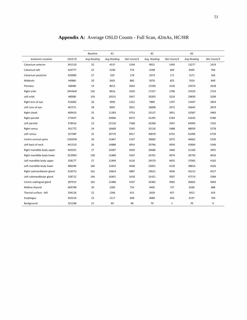
51

Appendix A: Average OSLD Counts - Full Scan, 42mAs, HC/HR

Baseline #1

#2

#3

Anatomic Location OSLD ID Avg Reading Avg Reading Net Count/3 Avg Reading Net Count/3 Avg Reading Net Count/3

Calvarium anterior 34151D 25 4537 1504 9021 1495 13277 1419

Calvarium left 42477T 22 2190 723 4198 669 6495 766

Calvarium posterior 42098X 27 559 178 1074 171 1571 166

Midbrain 44986I 20 2601 860 5076 825 7624 849

Pituitary 46848I 19 8012 2664 15590 2526 23474 2628

Right orbit 29436W 156 8916 2920 17257 2780 25429 2724

Left orbit 48908I 159 10531 3457 20203 3224 29830 3209

Right lens of eye 41606Z 26 3993 1322 7885 1297 13447 1854

Left Lens of eye 46757L 28 9091 3021 18008 2972 26645 2879

Right cheek 409410 25 11283 3753 23137 3951 33587 3483

Right parotid 27592Y 26 20946 6973 41295 6783 61635 6780

Left parotid 37841X 23 22126 7368 43268 7047 64994 7242

Right ramus 26177Z 24 16660 5545 33126 5488 48959 5278

Left ramus 32758P 25 20776 6917 40878 6701 61096 6739

Centre cervical spine 31835W 26 15467 5147 30682 5072 46662 5326

Left back of neck 44131D 26 14888 4954 29766 4959 45804 5346

Right mandible body upper 45032C 27 10287 3420 20686 3466 31160 3491

Right mandible body lower 35299O 158 12480 4107 24701 4074 36750 4016

Left mandible body upper 32817T 27 12404 4126 24570 4055 37065 4165

Left mandible body lower 48629K 160 13443 4428 25831 4129 38810 4326

Right submandibular gland 31657U 162 14824 4887 29631 4936 43213 4527

Left submandibular gland 32871Z 146 16401 5418 31421 5007 47574 5384

Centre sublingual gland 28791V 165 12486 4107 24382 3965 36662 4093

Midline thyroid 46970B 20 2283 754 4495 737 6560 688

Thyroid surface - left 294126 22 1266 415 2639 457 3912 424

Esophagus 35015A 23 2117 698 4084 656 6197 704

Background 321268 21 69 48 70 1 70 0

52

Appendix B: Average OSLD Counts - Full Scan, HC/HR

Baseline 14 mAs

28 mAs

Anatomic Location OSLD ID Avg

Reading

Avg

Reading

Net

Count/3

Average

Reading

Net

Count/3

Calvarium anterior 34151D 57 1305 416 3938 878

Calvarium left 42477T 62 671 203 1878 402

Calvarium posterior 42098X 55 195 47 485 96

Midbrain 44986I 60 818 253 2395 525

Pituitary 46848I 58 2401 781 7383 1661

Right orbit 29436W 55 2687 877 8048 1787

Left orbit 48908I 58 3096 1013 9387 2097

Right lens of eye 41606Z 54 1237 394 3719 827

Left Lens of eye 46757L 62 2816 918 8198 1794

Right cheek 409410 72 3723 1217 11005 2428

Right parotid 27592Y 65 6484 2140 19596 4370

Left parotid 37841X 59 6994 2312 21369 4792

Right ramus 26177Z 61 5221 1720 16129 3636

Left ramus 32758P 63 6212 2050 19539 4442

Centre cervical spine 31835W 59 4862 1601 15085 3408

Left back of neck 44131D 57 4945 1629 15421 3492

Right mandible body upper 45032C 63 3253 1063 9764 2170

Right mandible body lower 35299O 65 3966 1300 12306 2780

Left mandible body upper 32817T 63 3786 1241 11939 2717

Left mandible body lower 48629K 61 4180 1373 12941 2920

Right submandibular gland 31657U 60 4686 1542 14326 3213

Left submandibular gland 32871Z 61 4930 1623 15378 3483

Centre sublingual gland 28791V 56 3957 1300 12006 2683

Midline thyroid 46970B 58 729 223 2288 520

Thyroid surface - left 294126 50 512 154 1322 270

Esophagus 35015A 52 685 211 2100 472

Background 321268 52 56 4 58 2

53

Appendix C: Average OSLD Counts - Maxillary Scan, HC/HR

Baseline 14 mAs

28 mAs

42mAs


Reading Avg

Reading Net

Count/3 Avg

Reading Net

Count/3 Avg

Reading Net

Count/3


Calvarium left 42477T 62 691 210 2074 461 4045 657


Midbrain 44986I 63 811 249 2421 537 4845 808

Pituitary 46848I 63 2360 766 7409 1683 14856 2482

Right orbit 29436W 59 2575 839 7924 1783 16181 2752

Left orbit 48908I 60 3115 1018 9538 2141 19056 3173


Left Lens of eye 46757L 56 2741 895 8728 1996 17611 2961

Right cheek 409410 60 3640 1193 11025 2462 22151 3709

Right parotid 27592Y 67 6196 2043 19354 4386 38530 6392

Left parotid 37841X 54 6874 2274 20662 4596 40791 6710

Right ramus 26177Z 59 4965 1635 15084 3373 30711 5209

Left ramus 32758P 69 6055 1995 18960 4302 37425 6155












Esophagus 35015A 54 342 96 1053 237 2007 318

Background 321268 55 57 1 70 4 57 -4

54

Appendix D: Average OSLD Counts – Mandibular Scans, HC/HR

Baseline 14 mAs

28 mAs

42mAs


Reading

Avg

Reading

Net

Count/3

Avg

Reading

Net

Count/3

Avg

Reading

Net

Count/3


Calvarium left 42477T 67 154 29 370 72 672 101


Midbrain 44986I 64 205 47 559 118 1085 175

Pituitary 46848I 53 371 106 1127 252 2176 350

Right orbit 29436W 65 356 97 872 172 1756 295

Left orbit 48908I 61 372 104 982 203 2022 347


Left Lens of eye 46757L 68 194 42 517 108 973 152

Right cheek 409410 57 3157 1034 7540 1461 14233 2231

Right parotid 27592Y 69 5087 1673 15734 3549 31360 5209

Left parotid 37841X 71 5479 1803 17106 3876 34553 5816

Right ramus 26177Z 72 4417 1448 13677 3087 27206 4510

Left ramus 32758P 70 5552 1828 16783 3743 33672 5630












Esophagus 35015A 50 638 196 1760 374 3440 560

Background 321268 48 51 1 62 4 57 -2

55

Appendix E: Average OSLD Counts – Full Scans

Baseline

#1 NC/HR Baseline #2

HC/NR

NC/NR

Anatomic Location OSLD ID Avg Reading Avg

Reading Net

Count/3 Avg

Reading Avg

Reading Net

Count/3 Avg

Reading Net

Count/3

Calvarium anterior 34151D 3938 7888 1317 60 4793 1577 9179 1462

Calvarium left 42477T 1878 3873 665 61 2307 748 4459 717

Calvarium posterior 42098X 485 983 166 70 507 145 1036 177

Midbrain 44986I 2395 4821 809 63 2642 859 5151 837

Pituitary 46848I 7383 15020 2546 53 8042 2663 15743 2567

Right orbit 29436W 8048 16594 2849 61 8602 2847 17043 2814

Left orbit 48908I 9387 19223 3279 55 10033 3326 19828 3265

Right lens of eye 41606Z 3719 8339 1540 70 5677 1869 11785 2036

Left Lens of eye 46757L 8198 17432 3078 60 9376 3105 18130 2918

Right cheek 409410 11005 21724 3573 60 11908 3949 23086 3726

Right parotid 27592Y 19596 39577 6660 63 20596 6844 41125 6843

Left parotid 37841X 21369 45877 8169 61 21888 7276 43055 7056

Right ramus 26177Z 16129 31607 5159 61 16939 5626 33418 5493

Left ramus 32758P 19539 39728 6730 66 20044 6659 39572 6509

Centre cervical spine 31835W 15085 30368 5094 63 15463 5133 30561 5033

Left back of neck 44131D 15421 31345 5308 61 15083 5007 30760 5226

Right mand. body upper 45032C 9764 19446 3227 74 10849 3592 21301 3484

Right mand. body lower 35299O 12306 24222 3972 73 12568 4165 25156 4196

Left mand. body upper 32817T 11939 23750 3937 64 12267 4068 24397 4043

Left mand. body lower 48629K 12941 25711 4257 58 13154 4365 26007 4284

Right submand. gland 31657U 14326 28467 4714 58 14714 4886 29029 4772

Left submand. gland 32871Z 15378 31108 5243 62 15673 5204 31181 5169

Centre sublingual gland 28791V 12006 24046 4013 58 12370 4104 24684 4105

Midline thyroid 46970B 2288 4602 771 56 2173 706 4185 671

Thyroid surface - left 294126 1322 2677 452 63 1227 388 2542 438

Esophagus 35015A 2100 4132 677 64 2026 654 3957 644

Background 321268 58 54 -4 61 60 0 59 0

56

CURRICULUM VITAE

Name: David Richard Chambers

Post-secondary The University of Western Ontario

Education and London, Ontario, Canada

Degrees: 2011-2014 (expected) M.Cl.D

The University of Western Ontario


2000-2004 DDS

The University of Western Ontario


1996-2000 H.BSc. Pure Mathematics

Honours and The Joseph J. and Annie R. Kingston Gold Medal for Pure Mathematics

Awards: 2000

Continuing Entrance Scholarship, University of Western Ontario

1996-2000

University of Western Ontario Scholarship for Mathematics

1998

Related Work General Dentist, Civilian Contractor

Experience Canadian Forces Bases Borden, Kingston & Trenton

2004-2011

the effective dose of different scanning protocols using

Documents