The Effect of Welfare Reform on Women’s Marital Bargaining Power

By Mia Bird

A dissertation submitted in partial satisfaction of the

requirements for the degree of

Doctor of Philosophy

in

Public Policy

in the

Graduate Division

of the

University of California, Berkeley

Committee in charge: Professor Steven Raphael, Chair

Professor Rucker Johnson Professor Ronald Lee

Professor Jane Mauldon

Fall 2011

1

Abstract

The Effect of Welfare Reform on the Marital Bargaining Power of Women

Mia Bird

Doctor of Philosophy in Public Policy

University of California, Berkeley

Professor Steven Raphael, Chair

Marital bargaining models predict changes in the policy environment that affect the relative well-being of husbands and wives in divorce will indirectly affect the distribution of power within marriage. This study estimates the effect of 1996 welfare reform policies on the marital bargaining power of women with young children. Although the distribution of marital power cannot be directly observed, I utilize Consumer Expenditure data to infer shifts in bargaining power from changes in family demand. I first differentiate gendered patterns of consumption to create an indicator of relative bargaining power which I call the “male bias.” I then use policy variation over time and across states to identify the effect of welfare reform on the marital bargaining power of low-income women with young children. I characterize states as either “intensive” and “non-intensive” reformers based on 12 dimensions of welfare reform implementation policy. Based on these characterizations, I use a triple-difference estimator to capture the differential change in bargaining power for women with young children in intensive reform states. I estimate a 20 percentage point increase in the male bias for poor women and an 8 percentage point increase in the male bias for low-income women over the period of welfare reform. These findings suggest welfare reform caused a substantial decline in the marital bargaining power of those women most likely to view welfare as a potential alternative to marriage. Given evidence from the literature connecting women’s bargaining power with the share of family resources allocated toward children, these findings may have both equity and efficiency implications for further welfare policy reform.

i

Table of Contents

I. Introduction……………………………………………………………… 1 II. Demographic and Welfare Policy Context…………………………… 2

Creation of the Welfare Program………………………………………. 2 Expansion of the Welfare Program…………………………………….. 3 Introduction of Work Requirements and Child Support Enforcement… 6 The 1996 Welfare Overhaul……………………………………………. 9

III. Theory of Bargaining within Marriage……………………………... 11

Policy Implications of Bargaining Theory……………………………... 12

IV. Empirical Tests of Marital Bargaining……………………………... 13 Ownership of Wage Income…………………………………………... 13 Ownership of Non-wage Income……………………………………… 14 Changes in Divorce Laws……………………………………………… 15 Changes in Transfer Policy……………………………………………. 16

V. Methodology and Findings…………………………………………… 18

Research Design……………………………………………………….. 18 Data…………………………………………………………………….. 19 Construction of “Husband-driven” and “Wife-driven” Consumption

Categories………………………………………………………….. 21 Tests of Husband-driven and Wife-driven Consumption Categories…. 25 Change in Marital Bargaining Power over the Period of Welfare

Reform……………………………………………………………... 29 Characterization of States as “Intensive” and “Non-intensive”

Reformers…………………………………………………………... 34 Changes in Marital Bargaining Power in Intensive and Non-intensive Reform States………………………………………………………. 43 Change in Marital Bargaining Power for Lower-income Women with Young Children across Intensive and Non-intensive Reform States. 44 Change in Marital Bargaining Power for Lower-income Women with Young Children Living in Intensive Reform States over the Period of Welfare Reform…………………………………………………. 48 Summary of Findings…………………………………………………… 50

VI. Policy Implications……………………………………………………. 51

Implications for Evaluating Welfare Reform…………………………… 51 Implications for Making Future Policy………………………………… . 52

References…………………………………………………………………. . 53

ii

List of Figures

Figure 1. Welfare Caseloads: 1960-2010……………………………… 4 Figure 2a. Percent of Women Aged 15-29 Unmarried at First Birth by Race: 1930-1959…………………………………… ………. 5 Figure 2b. Percent of Women Aged 15-29 Unmarried at First Birth by Race: 1960-1994…………………………………… ………. 5 Figure 3. Percent of Children Living with Single Mothers by Marital Status of Mothers: 1960-1995………………………………. 7

Figure 4. Utilities Possibilities Frontier for Marriage, including Threat Points and an Equilibrium Outcome……………….... 12

iii

List of Tables

Table 1a. Sample Characteristics by Current Marital Status and Gender……………………………………………………… 20

Table 1b. Expenditure Shares by Current Marital Status and

Gender………………………………………………………. 21 Table 2a. Relationship between Gender and Proposed “Male-driven”

Consumption Categories…………………………………… 23 Table 2b. Relationship between Gender and Proposed “Female-driven”

Consumption Categories……………………………………. 24 Table 3a. Test of the Relationship between Gender and Constructs:

Full Sample……………………...…………………………. 27 Table 3b. Test of the Relationship between Gender and Constructs:

Sub-samples of Previously or Currently Married and of Widows and Widowers…………………………………….. 28

Table 4a. Differential Change in the Male Bias for Lower-income

Married Women with Young Children (1995-2000)……… 32 Table 4b. Differential Change in the Male Bias for Lower-income

Married Women with Young Children (1990-1996)……… 33

Table 5a. Work Requirement Policies…………………………… 37 Table 5b. Childbearing Policies………………………………….. 39 Table 5c. Income and Asset Limits……………………………… 40 Table 5d. Sanction and Diversion Policies………………………. 41 Table 5c. Lifetime Limits………………………………………... 42 Table 6a. Differential Change in the Male Bias for Lower-income

Married Women with Young Children Living in Intensive Reform States (1995-2000)……………………… 45

Table 6b. Differential Change in the Male Bias for Lower-income

Married Women with Young Children Living in Non-intensive Reform States (1995-2000)………………… 46

Table 6c. Differential Change in the Male Bias for Lower-income

Married Women with Young Children across all States (1995-2000)………………… ……………………………… 47

iv

Table 7. Differential Change in the Male Bias for Lower-income

Married Women with Young Children over Time and across States (1995-2000)………………………………….. 49

v

Acknowledgements

I am grateful for the support of the faculty and staff of the Goldman School of Public Policy. In particular, I’d like to thank my advisor, Steve Raphael, for the amazing guidance and opportunities he has offered me over these years. I would also like to thank Steve, along with Henry Brady, for their efforts to provide support and training to Ph.D. students through the IGERT program. The support and training I received through this program was essential to my success. I am also grateful to my dissertation committee members, Jane Mauldon, Rucker Johnson, and Ronald Lee. He many not know it, but this dissertation grew out of my first course with Ron. He was a wonderful supporter of my budding mind. While Rucker arrived somewhat later in my process, his contribution has been profound. Through his energy and investment in his work and his students, he has offered me a model of the kind of researcher and teacher I would like to become. There is no way I could thank Jane enough. She has been a steadfast supporter and role model, both as a person and a professor, from the beginning of my time as GSPP. In my first semester as a young MPP student, I took the course “Carrots and Sticks” with Geno Smolensky. We argued about almost everything and came to respect and appreciate each other. Geno sees the best in me and his confidence in my abilities has been essential to my progress. I cannot imagine how I would have achieved this goal or who I would be now without his influence and support. I appreciate the feedback of the participants in the Ph.D. seminar group at the Goldman School of Public Policy. I especially want to thank Sharyl Rabinovici for the tremendous role model and support she has offered me. I also want to thank Heidi Sommer, Erika Weissinger, and Sarah Martin-Anderson for being amazing women, friends, and professional supports to me through this process. I am grateful for the support of my friends and family. I want to especially thank my dear friends Jessica Leonard, Kelly McVicker, and Mia McKee, as well as my wonderful roommates Colleen Henry and Liz Garcia. Finally, I want to thank Sarah Lippman for her long-standing friendship and faith in me.

1

I. Introduction and Overview The desire to correct perverse incentives built into the social safety net drove much of the political will to reform welfare in the mid 1990’s. The story told by many liberal economists was one in which welfare offered benefits to needy families in the short-run, but made them worse off in the long-run by creating incentives for recipients to have more children and to remain unemployed and unmarried. Welfare reforms focused on reducing those incentives through the implementation of work requirements, time limits, family caps, and marriage promotion programs. Taken together, these reforms represent a shift from a social safety net for needy families to a temporary and limited public assistance program. Efforts to evaluate the impact of welfare reform primarily focus on the outcomes of a relatively small pool of current and former recipients and their families. However, the nature and existence of a social safety net also affects a much larger pool of families who may never need or receive public assistance. Given the persistent gender division of labor, a strong social safety net provides married women with children with an exit alternative to their marriages. Theory suggests women, particularly low-income women with young children, will have more marital bargaining power under a strong safety net system than under a weak one. Furthermore, empirical work has demonstrated that both women and children benefit from increases in intra-family resource allocations when women experience increases in their bargaining power. The indirect effect of welfare reform on this non-recipient group of women and children should be included in our analyses of the impacts of welfare reform and our overall understanding of the role of the social safety net in improving outcomes for families. The goal of this study is to estimate the effect of welfare reform on the marital bargaining power of low-income women with young children. While marital bargaining power is my outcome of interest, it operates within the black box of family decision-making and cannot be directly observed. Instead, I use changes in family consumption patterns to signal changes in the distribution of power between husbands and wives. I first differentiate observed consumption patterns that appear “male-driven” from those that appear “female-driven,” allowing us to infer the direction of changes in bargaining power from changes in family demand. I then utilize policy variation over time and across states to identify and estimate the differential effect of welfare reform on the marital bargaining power of low-income women with young children.

The paper proceeds as follows. Section II presents the demographic and policy context of welfare reform. Section III discusses the theory of marital bargaining power and its policy implications in this context. Section IV synthesizes and evaluates the relevant literature. Section V explains the research design and data, and presents findings. Finally, Section VI explores the policy implications of these findings.

2

II. Demographic and Welfare Policy Context The family has undergone significant change from the time that welfare was first enacted

and through the subsequent periods of reform into present-day policy. We now live longer, have fewer children, bear children later and increasingly out-of-wedlock, marry later and less frequently, divorce more often, and increasingly enter into sexual relationships and family formations that are alternatives to the traditional married couple with children. Our gender roles in families have also changed. The average education levels and labor force participation rates of women have increased dramatically relative to men, while the participation of men in the care of the home and children has increased somewhat as well. These changes in family demographics and economics have influenced the creation and evolution of welfare policies over time. Creation of the Welfare Program

The Aid to Dependent Children (ADC) program passed as one of the least controversial

components of the 1935 Social Security Act. ADC was created to provide income support for families with absent breadwinners. The legislation provided federal funds on a matching basis to support new and existing state and local level mothers’ pension programs. The initial funding came with little regulation or oversight from the federal government, leaving the targeting of these funds up to state and local discretion. As had been the practice prior to federal legislation, states and localities continued to restrict support to families with “deserving” mothers (typically white, widowed homemakers) who provided “suitable” homes (typically religious homes where men were never present) for their children (Gordon 1994). Thus, families needed to pass both means-test and a morality-test to qualify for welfare support.

With the passage of the 1939 Social Security Act Amendments, many poor widows became eligible for survivor’s support and, as a result, they no longer received support for their children through the ADC program. As these families left welfare, the caseload composition shifted increasingly toward mothers who had been abandoned by their husbands or who had never married. By 1942 only half the welfare caseload was made-up of widowed women and their children. As caseload composition changed, government became increasingly concerned with distinguishing between families who had lost fathers and husbands and those who had been abandoned by them. In 1950, states were instructed to notify law enforcement in cases in which support was granted to children who had been abandoned by their fathers. This legislation passed over 60 years ago was the first step toward a child support enforcement system.

Welfare caseloads remained low through the 1940’s and 1950’s because, in the absence

of federal standards, states and localities were able to discriminate in the provision of benefits (Chase-­‐Lansdale  and  Vinovskis  1995). They increasingly applied means-tests based on both current family income and ability to earn future income, limiting caseloads by defining some poor women as “employable” mothers whose ability to work outside the home disqualified their children from welfare support (Goodwin 1995). These distinctions between employable mothers and non-employable mothers were sometimes based in differences in prior work histories and highly correlated with race. Efforts to deem some mothers employable, particularly those who had worked in the fields or domestic service, were also linked to concerns (especially in the south) about maintaining the low-skilled (low-paid) labor pool.

3

The behavior of a few southern states was particularly egregious. For example, during this period in Arkansas otherwise eligible mothers were denied benefits at harvest time because they were deemed temporarily employable through the “farm policy” (Handler 1972). States and localities justified denying benefits based on employability in about half of the cases that were rescinded between 1953 and 1960 (Bell 1965).

During this period caseloads were also suppressed by denying or rescinding welfare

benefits to families that failed to pass the morality test. By 1950, 19 states had formed eligibility rules that excluded children based on their mother’s marital status at the time of their birth (Holcomb  1993).   In Louisiana welfare was rescinded for tens of thousands of children in the early 1960’s—90 percent of whom were black—due to a failure of their mothers to provide “suitable” homes (Mink 1995). Under similar eligibility rules as those used in Louisiana, Alabama disqualified more than 15,000 children from welfare support—again, 90 percent of whom were black—based on a “substitute father” rule that prohibited a family from receiving welfare if the mother was intimate with any able-bodied man. Expansion of the Welfare Program

One of the few federal regulations over the state administration of welfare in the 1935

Social Security Act was the requirement that no state rescind benefits to families without just cause. As a result, in 1961 Arthur Fleming, the head of the Department of Health, Education, and Welfare at the time, issued an administrative order that states could no longer rescind or deny welfare benefits to children whose homes were deemed “unsuitable.” Instead, states must either provide the necessary supports to make the home suitable, or remove children from the home and place them in a suitable home with additional supports. The order was passed as legislation by Congress a year later and resulted in an increase in welfare caseloads, and the issue made its way to the Supreme Court in 1968. The Court struck down the “substitute father” rule in Alabama based on an argument that the original intent of the welfare program, as expressed in the Social Security Act, was to aid families in which the natural father was not present. The Court further reiterated that welfare could not be denied to children “on the basis of their mothers’ alleged immorality or to discourage illegitimate births” (King v. Smith 1968).

Following King v. Smith, the Court took on the case of Vivian Thompson, a pregnant

mother in Connecticut who was denied welfare benefits because she had recently moved from another state (Shapiro v. Thompson). In its 1969 decision, the Court established a fundamental right to travel and ruled the state must grant Thompson welfare benefits. In the last and perhaps most important in this series of welfare rights victories, the Court ruled that welfare benefits could not be terminated without due process (Goldberg v. Kelly 1970). Specifically, that welfare benefits could not be rescinded without an evidentiary hearing before an impartial decision-making body.

4

Increase in Welfare Caseloads

The number of children and families who were able to access welfare benefits grew as states and localities were prohibited from using many of the discriminatory strategies that had allowed them to keep caseloads low in the past. In addition, the federal government further increased caseloads by extending welfare benefits to cover single parents (AFDC) and two-parent families in which the breadwinner was unemployed (AFDC-UP) in the early 1960’s. Caseloads also grew as the number of eligible families increased with the rate of non-marital childbearing. Figure 2 shows the dramatic increase in welfare caseloads during the 1960’s and 70’s. Between 1960 and 1975, the number of children receiving welfare nearly quadrupled and the family caseload more than tripled.

Increase in Non-marital Childbearing At the time ADC was enacted, the vast majority of women married before having children. In 1935 less than 10 percent of all women aged 15-29 were unmarried at the time of their first birth (see Figure 3a). However, rates of non-marital childbearing varied significantly by race. While only one in twenty white women had their first child out-of-wedlock, one in three black women were unmarried at the time of their first birth (Bachu 1999). These large racial differences in the relationship between marriage and childbearing allowed for states ostensibly applying a morality test for welfare support to effectively exclude eligible black mothers at much higher rates than eligible white mothers. This racial difference in the proportion of births outside marriage persisted through the 1940’s and 1950’s, but there was little change in non-marital childbearing overall.

5

6

The proportion of women aged 15-29 who were unmarried at the time of their first birth was about the same in 1959 as it had been in 1935. However, in the decades that followed the proportion of women who had their first birth while unmarried would increase dramatically—from one in ten younger women in 1960 to four in ten younger women in 1990—for all racial groups (see Figure 3b). By 1995, more than three-fourths of black women aged 15-29 had a non-marital first birth, compared to one-third of white women and two-fifths of Hispanic women. These three factors—legislation and court cases ending discrimination, extension of welfare benefits to cover single-parents and married couples with an unemployed breadwinner, and the increase in the proportions of women giving birth outside marriage—expanded eligibility and access, causing welfare caseloads to shoot up dramatically in the 1960’s and 1970’s. Caseloads would remain at or near this level through the following two decades, leading to a series of legislative efforts to reform welfare and, ultimately, to the welfare overhaul of the mid-1990’s and the subsequent rapid decline in caseloads back down to 1960’s levels (see Figure 2). Introduction of Work Requirements and Child Support Enforcement

As caseloads grew and caseload composition changed, concerns about welfare costs came

to the political forefront. In the 1940’s and 1950’s, states had been able to directly discriminate against mothers who they perceived as employable or unsuitable, a perception highly correlated with race, by denying them benefits. This discrimination served two purposes—it kept welfare costs low and it maintained the support of the political majority. As caseloads grew in the 1960’s and 1970’s, welfare costs and political calls for reform increased. Given the simultaneous nature of these two changes, it is difficult to separate out the role of cost concerns from the role of racial prejudice in motivating subsequent legislation.

Over this period, the number of families headed by single mothers grew due to increases in rates of both divorce and non-marital childbearing. Between 1960 and 1980, the proportion of children living with never married mothers tripled (from less than 5 percent to more than 15 percent), and the proportion living with divorced mothers nearly doubled (from less than 25 percent to more than 40 percent). By 1980, the majority of children in families headed by single-mothers either lived with mothers who had never married or mothers who had divorced (see Figure 4). Over the decades that followed, non-marriage approached divorce as a cause of single-motherhood.

These demographic changes fundamentally altered perceptions of the role of the welfare program in society. While welfare was initially framed as support for families who experienced hardship through no fault of their own, increased rates of divorce and non-marital childbearing suggested newly-eligible families had arrived at their circumstances through a series of choices rather than simply bad luck. The role of welfare in rewarding the immoral behavior of mothers and/or the deviant behavior of absent fathers gained an important political salience.

7

At the same time, the original premise of welfare—the assumption that the appropriate place for mothers was in the home—gradually weakened. Women’s labor force participation had increased by 50 percent over a twenty year period, from a rate of 29 percent of women in 1950 to 43 percent of women in 1970. This trend continued through the 1970’s, and by 1980 over half of all women were working. While in 1965 less than one-third of college age women stated they expected to be in the labor force at age 35, by 1980 over 80 percent of college age women expected to be working during their childbearing years (Goldin and Katz 2004). As middle-class mothers increasingly pursued work outside of the home, political support declined for providing benefits to poor single mothers so that they could remain in the home as caregivers. Work Requirements for Mothers

In response to changes in the roles of women and mothers, as well as increases in caseloads and changes in caseload composition, Congress established the Work Incentive and Training (WIN) Program through the 1967 Social Security Amendments. WIN required states to establish voluntary (made mandatory in 1971) employment and training programs for welfare recipients whose youngest child was six years or older. There were a range of intentions behind the WIN program. While some supported WIN with the hope that these programs would improve economic outcomes for participants, others supported the program with the hope that the additional requirements would deter families from participation. In either case, the original intention of the program—to support families with absent breadwinners—had fundamentally changed. The message sent by the legislation was that it was now not only appropriate for a single mother to take on the role of breadwinner, but it was required that she either do so or find man who would.

8

In spite of this message, the legislation did little to change life for most recipients. Funding was limited and states lagged in implementing programs and the associated requirements (Rein 1982). Caseloads and welfare costs continued to grow throughout the 1970’s. In 1981, Congress took further action to support the development and utilization of WIN programs. The Omnibus Budget Reconciliation Act encouraged and supported state education and training demonstrations. The legislation allowed states to require workfare—unpaid work in exchange for welfare benefits—of recipients for the first time and allowed states to use welfare funds to subsidize employment in the public sector. Under this legislation, Congress intended to use the states as research laboratories for the design of a successful national education, training, and work-incentive program.

Program evaluations showed modest effects of employment and training programs under

several of state demonstration programs (Nightingale and Holcomb 1997). Based (in part) on these findings, Congress required states to adopt the Job Opportunities and Basic Skills (JOBS) program through the 1988 Family Support Act. This legislation allowed states to extend work requirements to recipients with children age three and older. The legislation also provided additional federal matching grants to states to provide assistance for the childcare expenses of working recipients and allowed states to continue childcare support and Medicaid for one year after families left welfare. States were required to implement JOBS programs by 1991; by 1994, less than 15 percent of welfare recipients were enrolled in a JOBS program (Nightingale 1997). Although never fully funded or fully implemented, this program was soon replaced by the work requirements and state flexibility built into the 1996 welfare overhaul. Child Support Required of Fathers

Congress established the Office of Child Support Enforcement (OCSE) in 1975 through Title IV-D of the Social Security Act. The establishment of a federal and public enforcement system was an explicit response to increases in the proportion of children living in single-parent families and the associated welfare costs of providing support to a portion of those children. The new legislation required states to set up child support enforcement offices that met minimum standards, including the establishment of a parent locator system, and attached this requirement to the receipt of federal grants. These mandates expanded through the 1988 Family Support Act, which further required that states begin withholding the wages of delinquent non-residential fathers whose children received welfare support.

Efforts to recoup the public costs of welfare benefits from non-residential fathers would expand through the welfare overhaul of 1996. As a condition of assistance, welfare recipient mothers would be required (by threat of benefit sanctions) to report the paternity and location of non-residential fathers and to sign over their rights to receive child support to the state, allowing states to retain the full amount of child support to compensate for welfare costs. PRWORA would also eliminate the federal requirement that states disregard the first $50 in child support income received by recipient families.

9

The 1996 Welfare Overhaul Welfare caseloads grew rapidly in the early 1990’s. Between 1990 and 1994, caseloads increased by 1 million families (see Figure 1). Although efforts to implement comprehensive education and training for recipients through the JOBS program were only in the early stages of realization, concerns about welfare costs and perverse work, marriage, and childbearing incentives fueled calls for further reforms. In the 1994 congressional election Republicans ran on a “Contract with American” platform that included intensive reforms to the welfare program; they won majorities in both houses of Congress for the first time since the 1950’s. President Clinton had run for office two years earlier with a promise to “end welfare as we know it.” As the 1996 election cycle approached, pressure mounted for Congress to pass and for the President to sign substantial welfare reform legislation. After vetoing two earlier bills sent to him by Congress, Clinton signed the Personal Responsibility and Work Opportunity Reconciliation Act (PRWORA) into law in August of 1996. The legislation took effect in July of the following year. PRWORA ended welfare as an entitlement, replacing the AFDC program with Temporary Assistance for Needy Families (TANF). Under TANF, the federal government requires states to impose work requirements on recipients within two years of receiving benefits and restricts federal funding to a total of five years in the lifetime of any adult recipient. However, states have the flexibility to impose earlier work requirements and earlier lifetime limits on assistance, as well as the flexibility to allow for work exemptions for certain groups of recipients, such as pregnant women or new mothers. States have the authority to impose “family caps,” which deny benefits to children born while a family is already receiving welfare. If recipients fail to meet work (or any other) requirements of assistance, states also have the authority to sanction them by reducing their benefits or denying them benefits altogether. Finally, many states operate formal diversion programs that offer eligible recipients alternative temporary assistance in exchanged for giving up their welfare eligibility. Welfare reform legislation also significantly enhanced supports for families transitioning off of welfare. The program authorized additional funding for childcare assistance, although funding levels remained far below demand for the period under consideration. The legislation also delinked Medicaid from welfare and increased the income eligibility thresholds for public coverage. Supports for low-income non-recipient families also improved through increases in the minimum wage, expansions in the Earned Income Tax Credit (EITC), and increases in child support enforcement. These policy changes, in combination with a strong economy, led to dramatic welfare caseload reductions. Between 1995 and 2000, caseloads were cut in half. Sanctions, diversion policies, and family caps directly affected caseloads by reducing eligibility and access, while work requirements and lifetime limits indirectly affected caseloads by reducing the value of welfare to current and would-be recipients. By 2000, the number of families receiving assistance was close to 1960 levels, representing a near-complete roll-back in the expansions of the previous four decades.

10

The 1996 welfare overhaul was the final step in process of reforms meant to fundamentally alter the nature of the program as a social safety net for families headed by single mothers. Although many of the policies included in welfare reform were introduced in earlier legislation, the 1996 law created the mandates and incentives for states to fully implement these policies. Work supports for the poor or near-poor increased substantially, but this increase in transfers to the working poor was matched with a reduction in transfers to the non-working poor. Scholz, Moffitt, and Cowan find transfers to single-parent families were 45 percent lower in 2004 than they had been in 1993 (2009). Welfare was created to allow single mothers to care for their children in the home. The program now required single-mother recipients to find jobs and place their young children in some form of childcare. Alternatively, recipients are encouraged to find spouses to support them as caregivers. Welfare reform clearly impacted recipient families, but it may have also affected non-recipient women and children. To the extent that this policy change reduced the well-being of mothers outside of marriage, we would expect it to also induce a shift in marital bargaining power from wives to husbands. As a result, women and children in lower-income families may have experienced a reduction in their access to resources. The following section outlines the research design and data used to capture the effect of welfare reform on the bargaining power of lower-income women with young children.

11

III. Theory of Bargaining within Marriage Economic theories of the family have developed over time to predict and explain how policy changes impact demographic outcomes—such as rates of marriage, marital and non-marital childbearing, and divorce—and economic outcomes—such as household labor supplies and intra-family resource allocations. Early models of the family assume family members share the same preferences or have completely interdependent utilities (Samuelson 1956; Becker 1974, 1981). These models are categorized as common preference models because they assume that once married, partners drop their market-oriented selves at the threshold of the home and jointly maximize a single utility function relative to the family budget constraint, allowing for easy incorporation of the family into previously existing models of individual behavior. This assumption also suggests that family demand will not change in response to changes in the relative incomes of partners or their relative positions outside marriage. If we weaken the assumption that partners either share the same preferences or behave altruistically toward one another, we allow for individual utility functions to persist in the context of the family. A second set of models, game-theoretic bargaining models, assume husbands and wives behave as individuals with distinct preferences and bargain with each other to maximize their individual utilities within marriage (Manser and Brown 1980; McElroy and Horney 1981). These models do not preclude utility interdependence, but assume partners will bargain with each other to the extent that interdependence is incomplete. Under this assumption, shifts in the relative ownership of income would likely induce observable changes in family demand.

Bargaining models have evolved to incorporate relative utilities in divorce as ultimate

threat-points—boundaries to the marital negotiation process—from which each partner negotiates for a larger share of the marital gains. If the marital allocation is such that either partner receives less in marriage than he or she expects to receive in divorce and marital negotiation fails to produce a reallocation, then theory predicts that partner will initiate divorce. Figure 1 shows the utility possibilities frontier of a hypothetical couple. The divorce threat points (TPw, TPh) are shown for each partner as boundaries to the bargaining process and the utility levels experienced as the outcome of the bargaining process are shown as (Uw*, Uh*).

This couple may settle on an efficient position at any point along the frontier or an inefficient position at any point interior to the frontier (Lundberg and Pollack 1993). A potential egalitarian outcome (e*) is shown. Those partners with high threat points (high-value exit alternatives to marriage) are likely to have greater marital bargaining power than those with relatively low threat points (low-value exit alternatives to marriage). In those couples that do not share preferences for an egalitarian distribution, higher bargaining power translates into a larger share of the marital gains, which may include greater resource allocation and more leisure time. While this sharing rule may be established at the time of marriage, relative threat points will likely change over time as circumstances within and outside the marriage change, resulting in reallocations within the family.

12

Policy Implications of Bargaining Theory As partners make long-run decisions relating to their marriage, such as building relationships with relatives, completing educations, buying homes, having children, or participating in the labor market, their relative expected utilities in divorce may change. For example, if a wife increasingly withdraws from market work over the course of her marriage, her economic status will increasingly depend on the marital relationship. As a result, we might expect her bargaining power to decrease relative to that of her husband. Similarly, if partners choose to have children and the wife takes on the primary caregiving role, her economic alternatives to marriage become less desirable as she may need and want to provide care for their children if the couple were to divorce. On the other hand, the expected utility of divorce may fall for the husband relative to his wife after having children because he may expect to have less access to their children in divorce. Broad changes occurring outside the marriage, including changing divorce laws, social expectations, economic opportunities, and safety net supports, may also affect expected utility in divorce. Changes that reduce the costs of divorce for both partners will raise their threat-points and may lead to an increase in the overall divorce rate. However, changes that have an equivalent impact on the well-being of both partners in divorce should not induce a change in the distribution of power. Conversely, a policy change like welfare reform will likely induce a change in the distribution of marital bargaining power. As a result, we expect to see evidence of a reallocation of resources or leisure within families.

Wife’s Utility

Husband’s Utility

Uwmax

TPw

Uhmax TPh

e*

Figure 4. Utilities Possibilities Frontier for Marriage, including Threat Points and an Equilibrium Outcome

Uh*

Uw*

13

IV. Empirical Tests of Marital Bargaining Common preference models suggest that changes in the relative ownership of family income should have no effect on family demand or the allocation of leisure time, so long as these changes do not affect total family income, relative prices, or relative wages. In contrast, bargaining models suggest that changes in relative ownership of income will produce observable changes in family consumption patterns or time allocations. These different predictions provide an opportunity to empirically test how well each model explains behavior. Bargaining models also suggest the external environment affects marital bargaining power through its influence on the utility levels marital partners expect to experience in divorce. Therefore, if the bargaining model is correct, when policy changes benefit either husbands or wives, we should observe associated changes in the relative consumption of goods and leisure time. Ownership of Wage Income Two key studies have found important differences in family consumption depending on the relative ownership of wage income. Browning and colleagues (1994) use Canadian Expenditure Survey data from 1978-1986 to estimate the effect of relative income ownership on the family consumption of men’s clothing and women’s clothing. The advantage of using these two consumption categories as outcomes is that they are easily associated with the preferences of husbands and wives. Browning et al. use a sample of single adults to account for the potential endogenous relationship between higher-paid occupations and higher expenditures on clothing, and find individual incomes matter for husbands and wives in a way that income does not for single adults. Phipps and Burton (1998) set up their study as a test of the main restriction of common preference model, that family expenditure in any category is a function of the pooled income of the husband and wife given their demographic characteristics. They also use Canadian Expenditure Survey data (collected a decade later in 1992) to test the effects of differences in relative income on family demand. Rather than limiting their analysis to men’s and women’s clothing expenditures, however, they consider 14 categories of expenditure. They first estimate Engel curves for these categories to determine whether expenditure patterns are consistent with the assumption that consumption depends on the sum of the husband’s and the wife’s income. Phipps and Burton ultimately reject the pooling assumption for 7 of the 14 expenditure categories. They then generate iso-expenditure curves for those 7 categories, which show differences in the roles of the husband’s and wife’s incomes in driving consumption within each category. They find that when the husband’s income is relatively higher, family demand is higher for men’s clothing, transportation stock goods, and transportation flow goods; when the wife’s income is higher, family demand is higher for women’s clothing, children’s clothing, childcare, and restaurant meals. In particular, childcare expenditures appear entirely driven by the level of the wife’s income, suggesting a separate spheres orientation even among the dual-earner couples they consider. These findings provide both support for the bargaining model and a basis for inferring gendered patterns in consumption.

14

The findings of Browning et al. and Phipps and Burton suggest bargaining models of family behavior have stronger explanatory power than common preferences models. However, observed differences in earned income are likely endogenous to past and present household choices. These authors deal with this issue, in part, by limiting their samples of married couples to partners who both have positive work hours (Browning et al.) or who both work full-time, year-round (Phipps and Burton). However, these choices by couples are likely endogenous to the distribution of marital bargaining power. Ownership of Non-wage Income Non-wage income is arguably exogenous and, therefore, may provide a better test than wage income of the effect of the relative ownership of income on family demand. Schultz (1990) uses 1981 Socioeconomic Survey data from Thailand to test the gendered effect of increases in non-wage income on labor supply and fertility. He finds an increase in a woman’s own non-wage income reduces her labor supply by six times that of the same increase in her husband’s non-wage income. He also finds increases in women’s non-wage income led to increases in fertility. This finding is somewhat surprising because the costs of childbearing are disproportionately born by women, while the benefits are thought to be shared by men and women. Schultz challenges this notion in the social, cultural, and historical context in which the data was gathered. He highlights the key difference between using observed indicators of changes in bargaining power to simply reject the pooled income hypothesis, and the more complex task of drawing normative conclusions based on the direction of those shifts. Thomas (1990) also tests the gendered effect of increases in non-wage income. He uses data collected on Brazilian family income and expenditures for the years 1974-1975 to estimate the effect of non-wage income ownership on consumption and fertility. He finds non-wage income in the hands of mothers has a much larger effect on family health expenditures and health status than the same amount of non-wage income in the hands of fathers. Specifically, he estimates the effect of non-wage income on child survival likelihoods is 20 times greater when the income is received by mothers compared to when the income is received by fathers. In the Brazilian context, Thomas finds increases in non-wage income led to fertility reductions no matter which partner receives the income, but reductions in fertility were more strongly associated with increases in the non-wage income of women than with increases in the non-wage income of men. Klawon and Tienfenthaler (2001) also measure the effect of non-wage income on fertility using Brazilian data (collected in 1989). Their results are consistent with those of Thomas (1990); they find an increase in women’s non-wage income is associated with a larger reduction in fertility than an equivalent increase in men’s non-wage income. This effect was especially strong for increases in the non-wage income of the least educated women, suggesting policies that increase women’s bargaining power are likely to lead to fertility reductions, at least for Brazilian families. These three studies provide further support for bargaining models, as well as evidence that the balance of power between husbands and wives may have implications for the health and well-being of children. However, given the pervasiveness of gender roles in families across contexts, these studies do not allow us to sort out the effect of the sex of the parent from the effect of the gendered role of the parent in allocating increased resources toward children. From

15

a theoretical perspective, it is important to maintain this distinction. Non-wage income is still somewhat problematic as an exogenous influence on bargaining power. Some forms of non-wage income are arguably tied to past or current allocation decisions, such as income from held assets, pensions, social security, and workers compensation. Other forms of non-wage income, like inheritances and gifts, suffer less from endogeneity problems, but one-time increases in income may also affect consumption behavior differently from long-term streams of non-wage income. These challenges, in addition to an interest in evaluating policy outcomes, have led researchers to look to changes in the policy environment for exogenous shifts in bargaining power. Changes in Divorce Policy The structural environment outside the family impacts the relative utility levels of husbands and wives in divorce. If the bargaining model holds, changes in divorce policy that (on average) either benefit husbands or benefit wives will induce shifts in marital bargaining power. Gray (1998) uses the Census, CPS, and PSID to test for an effect of changes in divorce laws on female labor supply in the 1970’s. He characterizes some policy changes as beneficial to wives relative to husbands and others as beneficial to husbands relative to wives. Using state variation in divorce policy, he finds evidence that changes favoring women led to an increase in women’s market labor hours and a decrease in their home production hours, netting to a small overall increase in their leisure time. This study again highlights the difficulties of inferring women’s preference—in this case for market labor v. home production—and the important role the social and historical context may play in shaping the realization of those preferences. It also highlights the importance of capturing the often invisible work in the home in utilizing labor hours as an indicator of the effect of income or policy changes on marital bargaining power. Chiappori et al. (2002) also utilize variation across states in divorce laws to examine the effect of the environment outside marriage on intra-marital resource allocation. They create an index of four laws they characterize as favorable to women. The higher the index, the more favorable a state’s policies are towards women. Using PSID data from 1988, they find living in a state with one additional favorable divorce law was associated with a reduction in wives’ labor supply and an increase in husbands’ labor supply, suggesting favorable laws increase wives’ bargaining power and allow them to increase their leisure time relative to their husbands. An alternative but consistent interpretation is that more favorable divorce policies reduce the losses women experience from withdrawing from the labor force to, for example, care for children. Rangel (2006) also utilizes changes in divorce policy as a natural experiment. He uses Brazilian data from 1992-1995, a period in which the marital alimony policy was extended to cover unmarried women in cohabitating relationships. Rangel estimates the differential effect of this policy change on the labor supply of cohabitating women relative to married women over the period. He finds cohabitating women increased their leisure time overall by reducing both their market and non-market work hours. He also finds the expansion of alimony rights led to an increase in the probability that daughters would continue with their schooling, suggesting an increase in resource allocation toward children.

16

These studies are consistent with studies of wage and non-wage income effects in their support of marital bargaining over common preference models. They also confirm the role of the external environment in inducing changes in the intra-family allocation of goods and leisure time and provide further evidence that the balance of bargaining power between husbands and wives has implications for the wellbeing of children. Changes in Transfer Policy Changes in the allocation of cash transfers to families are perhaps more feasible as a policy tool to influence bargaining power than are changes in divorce laws. To the extent that they are unanticipated, changes in the ownership of non-wage income induced through policy changes in transfer payments are likely to be exogenous and serve as the best tests of the effect of income ownership on marital bargaining power. These studies may also allow us to infer differences in gender preferences for consumption. Lundberg, Pollak, and Wales (1997) take advantage of a shift in the parental ownership of a child subsidy in the United Kingdom in the 1970’s. This policy replaced a child-based tax deduction in the form of a higher paycheck for fathers with a child-based subsidy mailed directly to mothers. Using data form the U.K. Family Expenditure Survey (1973-1983) to measure changes in family demand, the authors find evidence in support of marital bargaining models. Specifically, they find an increase in expenditures on women’s and children’s goods relative to men’s goods, suggesting the shift in income ownership induced a shift in bargaining power and that mothers’ chose to utilize this increase in power to allocate additional resources to themselves and their children. Similarly, Duflo (2003) utilizes changes in the introduction of a government policy to extend pension benefits to black South Africans (who had formerly been excluded due to racial discrimination) to test the gendered effects of income ownership on family demand. Using data collected through a 1993 World Bank survey, she finds that increases in grandmothers’ non-wage income through receipt of these pensions led to health and nutritional improvements for their grandchildren. Duflo finds increases in grandfathers’ income through the same pensions had no effect on grandchild outcomes, suggesting preferences of grandmothers and grandfathers differ with respect to expenditures on grandchild health and nutrition. Finally, Bobonis (2009) estimates the effect of the ownership of cash transfers on family demand. Progressa, an innovative conditional cash transfer program, was implemented in the late 1990’s in Mexico. The program gave poor mothers cash transfers under the conditions that their children attend school and receive healthcare. Extensive evaluation data was collected, and Bobonis used this data (1997-1999) to estimate the effect of the arguably exogenous increase in the non-wage income of mothers on family demand. He finds this increase in women’s ownership of family income resulted in increased spending on children’s goods relative to an exogenous change in family income overall (due to the effect of variation in localized rainfall on family agricultural income).

17

The studies discussed here provide strong empirical evidence in support of bargaining models. The research also suggests that a range of policy decisions may have profound impacts on intra-family resource allocations. The underlying theoretical framework of this paper relies on a bargaining model of the family and the empirical evidence that shifts in bargaining power induce changes in family demand. I apply this framework to an analysis of the impact of the 1996 overhaul of welfare, the primary cash transfer program that supports poor women and their children.

18

V. Methodology and Findings The goal of this study is to estimate the effect of welfare reform on marital bargaining power. While bargaining power is my outcome of interest, it operates within the black box of family decision-making and cannot be directly observed. Instead, I use changes in family consumption patterns to signal changes in the distribution of power between husbands and wives. I first differentiate observed consumption patterns that appear “male-driven” from those that appear “female-driven,” allowing us to infer the direction of changes in bargaining power from changes in family demand. I then utilize policy variation over time and across states to identify the differential effect of welfare reform on women’s marital bargaining power. Research Design

Because the consumption preferences of couples are executed jointly in their family

expenditures and cannot be independently observed, I utilize the expenditure patterns of families headed by one adult to infer gender differences in consumption preferences. After controlling for a set of observed characteristics, I find large and significant gender differences in the expenditure behavior of families headed by single adults. Based on these differences, I sum expenditure categories associated with male consumption and designate increases in family expenditures within those categories as “male-driven.” I also sum expenditure categories associated with female consumption and designate increases in family expenditures within those categories as “female-driven.” Clearly, married men and women may be selected in ways that affect their consumption preferences relative to their single counterparts. To address this possibility of selection bias, I restrict the sample to single adults who are widowed. The gender differences remain large and significant.

I then estimate the effect of welfare reform on marital bargaining power using the time

period over which welfare reform was implemented at the national level. I identify lower-income married women with young children as the group most vulnerable to changes in welfare policy. I estimate the change in bargaining power for these women relative to other married women over the period of reform and find large and significant differential reductions in their bargaining power. I then conduct the following falsification test. I use the same model to estimate the differential change in bargaining power for this subgroup of women over the period prior to welfare reform (1990-1996). During this period, I find evidence of differential increases in the bargaining power of this subgroup of women. These findings demonstrate a trend of increasing bargaining power pre-reform and decreasing power post-reform, suggesting welfare reform at the national level changed the direction of the trend. However, it is possible that a change in some other important factor drove the differential change in bargaining power we see over the reform period.

To precisely identify the effect of welfare reform on marital bargaining power, I use

variation in policy implementation across states. I use 12 dimensions of welfare policy implementation to qualitatively characterize states as “intensive” reformers and “non-intensive” reformers. Based on these characterizations, I restrict the sample to intensive reform states and estimate the differential change in marital bargaining power for lower-income women with young children over the reform period. I find very large and significant effects for those living in

19

intensive reform states. I then restrict the sample of married couples to those living in non-intensive reform states. I estimate the differential change in bargaining power for the subgroup of women and find no evidence of an effect of welfare reform. I then return to the original sample and restrict the observations to include only lower-income women with young children. I estimate the differential effect of living in an intensive reform state over the period, and I find very large, significant changes in the bargaining power for women in intensive reform states relative to those in non-intensive reform states.

Finally, I return to the full sample of married couples and estimate the differential change

in bargaining power for lower-income women with young children in intensive-reform states over the period of welfare reform. Using a triple-difference estimator, I find large and significant effects of welfare reform. Based on these findings, I conclude that the weakening of the social safety net through welfare reform reduced the marital bargaining power of those women most likely to consider welfare as a possible exit alternative to marriage. Data The Consumer Expenditure Survey (CEX) collects annual expenditure data (on a quarterly basis) and member characteristics for cross-sectional samples of families. I pool CEX data from 1995 through 2000 to capture the time period in which welfare reform was enacted and implemented. I exclude households headed by students and those households with heads over the age of 50. This age exclusion is intended to create a sample of households with a reasonable likelihood of having young children present. I then isolate families headed by single adults (10,243) and married couples (12,630). Table 1a summarizes descriptive characteristics of these families by gender and family type. We see interesting but unsurprising differences in mean characteristics in the sample by gender and by family type. Single adult men and women are younger than their married counterparts. They are also more likely to be black and less likely to be white or Hispanic. Given the increasing average age of marriage and racial divergence in marriage rates we observed earlier in this paper, these findings are not surprising. We see that married men tend to be less educated than their single counterparts, a factor that is likely related to the education-marriage delay. The relationship between education and family type is less clear for women. Given the stabilizing effect of men’s educational attainment on marriage (and the potentially destabilizing effect of women’s education) these differences in characteristics appear consistent with the literature (Becker et al. 1977).

Married couples are more likely to have children than single adult family heads, but

single women are much more likely than single men to have children in their homes. Given the ratio of the number of potential earners in a family to the number of family members along with the lower average earnings of women relative to men, we would expect to see that the average family headed by a single woman is poorer than the average family headed by a single man. The average married couple has the highest income relative to their family size. Finally, we see small differences in urbanicity and across regions by gender and family type.

20

Table 1a. Sample Characteristics by Current Marital Status and Gender Men Women Married* Single Married* Single Age 37.2 33.1 35.4 33.4 Race and Ethnicity White 88.0% 84.3% 87.8% 71.7% Black 7.2% 10.1% 6.7% 23.8% Asian 3.9% 4.1% 4.4% 2.9% Hispanic 11.2% 6.9% 11.6% 9.4% Education Less than High School 11.3% 8.0% 10.9% 13.3% High School or GED 30.7% 23.7% 30.2% 26.2% Some College 27.1% 38.4% 30.4% 34.9% Bachelors Degree 20.0% 21.3% 20.0% 17.4% Graduate Degree 10.6% 8.5% 8.2% 7.9% Marital Status** Married 100.0% 2.6% 100.0% 2.6% Widowed 0.0% 1.3% 0.0% 3.8% Divorced 0.0% 24.9% 0.0% 29.2% Separated 0.0% 6.3% 0.0% 10.8% Never Married 0.0% 64.8% 0.0% 53.3% Children Any Children 77.4% 8.0% 77.4% 48.3% Young Children 32.5% 1.1% 32.5% 16.6% Older Children 44.8% 6.9% 44.8% 31.7% Family Size 3.6 1.1 3.6 1.96 % Poverty Line 3.8 3.4 3.8 2.2 Urbanicity Large City 49.9% 48.7% 49.9% 50.9% Small City 26.0% 27.1% 26.0% 26.8% * The means of household level variables will be the same for married men and married women. ** Note that some single adults are currently married but not living with their marital partners.

Given these differences in characteristics and the assumption that married couples must

bargain with each other to form their consumption bundles, it is not surprising that the consumption patterns of married couples are somewhat different from those of single men and single women in nearly every category of expenditure. Table 1b summarizes the average expenditure share of each household type by expenditure category.

21

Table 1b. Expenditure Shares by Current Marital Status and Gender Married Couples Single Women Single Men Home Meals 12.5% 14.9% 11.6% Restaurant Meals 3.7% 3.6% 5.8% Alcohol & Tobacco 1.7% 2.1% 4.0% Housing & Household Services 33.3% 39.5% 34.2% Vehicles & Transportation 18.5% 13.6% 15.7% Insurance & Pensions 12.5% 7.8% 10.6% Education 1.7% 2.4% 3.1% Health Care 4.2% 3.1% 2.5% Personal Care 0.9% 1.1% 0.7% Entertainment 5.1% 4.5% 5.7% Men’s Clothing 0.9% 0.2% 1.8% Women’s Clothing 1.0% 2.4% 0.1% Children’s Clothing 1.2% 1.3% 0.2% Miscellaneous Expenditures 2.6% 2.9% 3.5%

Before controlling for differences in the characteristics of these households, we see that single men, on average, spend higher shares of their incomes on restaurant meals, alcohol and tobacco, and men’s clothing relative to other households. In contrast, single women dedicate higher shares of their spending to housing and household services, personal care, and women’s clothing. Interestingly, the expenditures of married households often look like some combination of the expenditure preferences of single men and single women. In theory, this mixture would depend on the relative bargaining power of the husband and the wife in each couple. While we are unable to directly observe the distribution of bargaining power within these families, we may be able to infer changes in relative bargaining power from changes in consumption patterns. This observation becomes meaningful to the extent we are also able to determine the direction of such changes in marital power.

Construction of “Male-driven” and “Female-driven” Consumption Categories

I utilize the sample of families headed by single adults to determine how the consumption

behaviors of single men differ from those of single women. Equation (1) shows the regression model used to estimate the relationship between gender and each of the following expenditure categories: home meals, restaurant meals, alcohol and tobacco, housing and household services, vehicles and transportation, pensions and insurance, education, health care, personal care, entertainment, men’s clothing, women’s clothing, and children’s clothing. (1) ExpSharej = β0 + δ0male + βkXik + µ I regress each category of expenditure listed in Table 1b on gender, as well as variables representing age, race and ethnicity, education level, income as a percent of the poverty line, presence and age of children, and urbanicity. By including these demographic and economic variables, I control for the observable differences in the characteristics of single men and single women that may have an independent impact on their expenditure patterns.

22

Table 2a presents regression results for those expenditure categories positively associated with men. Table 2b presents regression results for those expenditure categories negatively associated with men and, therefore, positively associated with women. I find that men devote significantly higher proportions of their total expenditures to restaurant meals, alcohol and tobacco, vehicles and transportation, entertainment, pensions and insurance, and men’s clothing. In contrast, men devote significantly smaller shares of their total expenditures to housing and household services, health care, personal care, women’s clothing, and children’s clothing. I find no significant relationship between educational expenditures and gender. I find a small (about one-half of a percentage point) positive relationship between male household heads and expenditures on home meals. However, I exclude this expenditure category because gender differences in basic food consumption may be based in average differences in required caloric intake. I also find a small (about one half of a percentage point) gender difference in the reporting of miscellaneous expenditures, but exclude this category from analysis because it has little interpretive value.

These findings are consistent with the expenditure categories assigned to married men

and women by Phipps and Burton (1998).They are also consistent with the positive association in the literature between women’s control over resources and spending on women’s and children’s clothing (Lundberg, Pollack, and Wales 1997; Bobonis 2009) and health care (Thomas 1990; Duflo 2003). While differences in spending on men’s and women’s clothing are clearly related to the gender of the family head and may not reflect differences in underlying demand, other differences in demand may indicate differences in the underlying preferences of men and women or differences in social roles or circumstances highly correlated with gender and unobserved here.

I use the results presented in Tables 2a and 2b to construct “male-driven” consumption

(which sums family expenditures in those categories positively associated with male-headed households), and “female-driven” consumption (which sums family expenditures in those categories negatively associated with male-headed households). These categories are preliminary. I then test the extent to which these summary categories are appropriately associated with gender. I also test the extent to which these gender associations persist in the subsamples of single adults that are the most like the sample of married couples. Finally, I test for change in these gender associations over the time period of interest.

23

Table 2a. Relationship between Gender and Proposed “Male-driven” Consumption Categories Restaurant Alcohol & Vehicles & Entertainment Insurance Men’s Meals Tobacco Transportation & Pensions Clothing Intercept 6.09** 2.50** 14.93** 7.25** 3.76** 0.98** (0.27) (0.25) (0.88) (0.31) (0.39) (0.11) Male 1.64** 1.48** 1.27** 0.89** 0.53** 1.54** (0.10) (0.09) (0.32) (0.11) (0.14) (0.04) Age -0.06** 0.00 -0.02 -0.06** 0.08** -0.02** (0.01) (0.00) (0.02) (0.01) (0.01) (0.00) Black -0.84** -1.22** -2.15** -1.07** -0.04 0.16** (0.12) (0.11) (0.40) (0.14) (0.18) (0.05) Asian 0.49** -0.81** -1.41* -0.97** -0.19 -0.05 (0.23) (0.22) (0.78) (0.27) (0.34) (0.10) Hispanic -0.15 -1.56** -0.34 -0.82** -0.13 0.19** (0.16) (0.15) (0.54) (0.19) (0.24) (0.07) Less than HS -0.75** 2.86** -2.43** -0.89** -2.33** -0.20** (0.21) (0.20) (0.71) (0.25) (0.31) (0.09) High School -0.33* 1.86** 1.01* -0.44** -0.83** -0.21** (0.18) (0.17) (0.60) (0.21) (0.27) (0.08) Some College -0.04 1.22** 1.53** 0.06 -1.20** -0.13* (0.17) (0.16) (0.57) (0.20) (0.25) (0.07) Bachelors Degree 0.10 0.48** 1.28** 0.09 -0.09 -0.13* (0.18) (0.17) (0.59) (0.21) (0.26) (0.08) Children -0.17 -0.79** 1.91** 0.37* -0.27 -0.01 (0.19) (0.18) (0.63) (0.22) (0.28) (0.08) Young Children -1.05** -0.18 -2.49** -0.75** 0.37 -0.37** (0.17) (0.16) (0.58) (0.20) (0.26) (0.07) Family Size -0.10 -0.21** -0.57** 0.12 -0.51** 0.02 (0.08) (0.07) (0.26) (0.09) (0.11) (0.03) % Poverty Line 0.05** -0.14** 0.20** 0.06** 1.38** 0.01 (0.02) (0.02) (0.06) (0.02) (0.03) (0.01) Large City 0.33** 0.01 -1.23** -0.68** 0.34** 0.06 (0.11) (0.10) (0.37) (0.13) (0.16) (0.05) Small City 0.17 -0.17 -0.53 -0.47** 0.35** -0.01 (0.12) (0.11) (0.40) (0.14) (0.18) (0.05) R2 0.10 0.11 0.02 0.04 0.37 0.17 N 10,243 10,243 10,243 10,243 10,243 10,243 * significant at p < .10; ** significant at p < .05

24

Table 2b. Relationship between Gender and Proposed “Female-driven” Consumption Categories Housing Health Personal Women’s Children’s & Household Care Care Clothing Clothing Intercept 39.23** 1.19** 1.25** 4.30** 0.30 (0.87) (0.26) (0.08) (0.15) (0.10) Male -4.24** -0.74** -0.36** -2.95** -0.15** (0.32) (0.10) (0.03) (0.05) (0.04) Age 0.15** 0.09** -0.01** -0.03** -0.01** (0.02) (0.01) (0.00) (0.00) (0.00) Black 2.77** -0.64** 0.83** -0.07 0.63** (0.39) (0.12) (0.03) (0.07) (0.05) Asian 3.39** -0.77** 0.00 -0.13 0.11 (0.77) (0.23) (0.07) (0.13) (0.09) Hispanic 2.45** -0.44** 0.06 0.04 0.08 (0.53) (0.16) (0.05) (0.09) (0.06) Less than HS 0.62 -0.78** -0.19** -0.34** 0.54** (0.70) (0.21) (0.06) (0.12) (0.08) High School -1.13* -0.39** -0.08 -0.11 0.24** (0.59) (0.18) (0.05) (0.10) (0.07) Some College -1.98** -0.19 -0.04 0.20 0.04 (0.57) (0.17) (0.05) (0.10) (0.07) Bachelors Degree -0.37 0.27 0.00 0.13 0.00 (0.59) (0.18) (0.05) (0.10) (0.07) Children -0.84 1.02** 0.03 -0.60** 0.78** (0.63) (0.19) (0.06) (0.11) (0.08) Young Children 4.63** -0.45** -0.22** -0.49** 0.93** (0.57) (0.17) (0.05) (0.10) (0.07) Family Size -0.82** -0.46** 0.04* -0.27** 0.47** (0.25) (0.08) (0.02) (0.04) (0.03) % Poverty Line -0.58** -0.05** -0.01 0.04** 0.01 (0.06) (0.02) (0.00) (0.10) (0.01) Large City 3.18** -0.34** 0.08** 0.08 0.07 (0.36) (0.11) (0.03) (0.06) (0.04) Small City 0.89** 0.08 0.03 0.09 0.07 (0.40) (0.12) (0.04) (0.07) (0.05) R2 0.07 0.06 0.09 0.24 0.32 N 10,243 10,243 10,243 10,243 10,243 * significant at p < .10; ** significant at p < .05

25

Tests of Male-driven and Female-driven Consumption Categories After constructing the categories of male-driven and female-driven consumption, I use

the following regression models to test the relationship between the gender of the single adult family head and the share of family expenditure in these consumption categories: (2) Male-driven share = β0 + δ0male + βkXik + µ

(3) Female-driven share = β0 + δ0male + βkXik + µ In model (2), I regress the male-driven share on gender and the full set of controls. I find a large and significant relationship—families headed by men devote an estimated 7.35 percentage points (p=.00) more of expenditures toward male-driven goods. In model (3), I regress the female-driven share of consumption on gender and the full set of controls. I find a large and significant relationship—families headed by women devote an estimated 8.44 percentage points (p=.00) more of expenditures toward female-driven goods. Table 3a presents these findings along with the full set of control coefficients. We see a small negative relationship between age and male-driven consumption and a small positive relationship between age and female-driven consumption. Families headed by adults who are Black, Asian, or Hispanic devote smaller shares of their expenditures toward male-driven goods and larger shares toward female-driven goods relative to those with White family heads. While, on average, family heads with lower education levels spend more on male-driven goods and less on female-driven goods. We see that having young children and living in urban areas are characteristics positively associated with higher shares of female-driven goods. These relationships between the control variables and the summary categories are generally consistent with the results presented for each consumption category in Tables 2a and 2b.

I then test the male-driven and the female-driven constructs against possible bias due to

selection into marriage. I limit my sample to families headed by single adults who are currently or were formerly married (4,260 families). I use models (2) and (3), and I find the gender differences in consumption persist. These differences are similar in magnitude to those in the full sample of single adults. Men spend an estimated 7.05 percentage points (p=.00) more on goods classified as male-driven. In contrast, women spend an estimated 8.07 percentage points (p=.00) more on goods classified as female-driven. Table 3b presents these results.

The decision to disrupt a marriage may be endogenous to the degree to which consumption preferences are highly gendered in the marital partners. To the extent that the adults in this group negatively selected out of the marital family relationship based on their consumption preferences, these estimates will still suffer from selection bias. To address this potential source of bias, I further limit by sample to families headed by widows or widowers (280 families). I run models (2) and (3) on this sub-sample and find results consistent in both direction and magnitude with the findings for the currently or previously married group. Specifically, men spend an estimated 7.03 percentage points (p=.00) more on male-driven goods, and women spend an estimated 8.35 percentage points (p=.00) more on female-driven goods (see Table 3b). This restricted sample is as close as we can get to married couples, as these adults

26

married and experienced a (presumably) exogenous shock that left them in single-headed families. Given these findings, I conclude the constructs are valid and proceed.

My final test addresses the possibility of change over time in the relationship between

gender and consumption patterns. I limit my sample to data from the pre-reform (1995/1995) and post-reform (1999/2000) periods, leaving a total of 7,278 families headed by single adults. I use the following regression models to test for differential changes in the expenditure shares devoted to male-driven and female-driven consumption, respectively: (4) Male-driven share = β0 + δ0male + β1post + δ1male*post + βkXik + µ (5) Female-driven share = β0 + δ0male + β1post + δ1male*post + βkXik + µ

If the relationship between the gender of the household head and the share of consumption devoted to male-driven goods was changing over time—perhaps due to some gendered change in the characteristics of the single adult populations or change in gender norms that affect preferences—then we would expect the coefficient on the interaction term to be either negative (men are spending less on male-driven goods in 1999/2000 than they were in 1995/1996) or positive (men are spending more on male-driven goods in the later period), and significant. Model (5) estimates this effect for the female-driven share of expenditure. I estimate small and non-significant δ1 coefficients for both models.

Based on these tests, I conclude that these constructs represent gendered patterns in

consumption and that there is no change in this pattern over time among single adults. I then use these constructs to create a single measure to capture changes in the relative bargaining power of husbands and wives. I define the “male bias” as the difference between the male-driven expenditure share and the female-driven expenditure share. A positive change over time in the “male bias” indicates a shift in household expenditures toward male-driven goods, reflecting an increase in the relative bargaining power of husbands. A negative change over time in the “male bias” indicates a shift in household expenditures toward female-driven goods, reflecting an increase in the relative bargaining power of wives. The “male bias” construct will be used throughout the analysis to indicate the direction and magnitude of changes in marital bargaining power.

27

Table 3a. Test of the Relationship between Gender and the Constructs: Full Sample “Male-driven” Share “Female-driven” Share Intercept 35.51** 41.96** (0.94) (0.87) Male 7.35** -8.44** (0.34) (0.32) Age -0.08** 0.18** (0.02) (0.02) Black -5.16** 3.53** (0.42) (0.40) Asian -2.94** 2.60** (0.83) (0.77) Hispanic -2.80** 2.18** (0.57) (0.53) Less than HS -3.73** -0.14 (0.75) (0.70) High School 1.06* -1.47** (0.64) (0.60) Some College 1.43** -1.97** (0.61) (0.57) Bachelors Degree 1.72** 0.04 (0.63) (0.59) Children 1.05 0.39 (0.68) (0.63) Young Children -5.21** 4.40** (0.62) (0.58) Family Size -1.24** -1.05** (0.27) (0.25) % Poverty Line 1.56** -0.59** (0.06) (0.06) Large City -1.19** 3.06** (0.39) (0.37) Small City -0.66 1.16** (0.43) (0.40) R2 0.24 0.14 N 10,243 10,243 * significant at p < .10; ** significant at p < .05

28

Table 3b. Test of Relationship between Gender and the Constructs: Sub-samples of Previously or Currently Married and of Widows and Widowers Previously or Currently Married Widow/Widower “Male-driven” “Female-driven” “Male-driven” “Female-driven” Share Share Share Share Intercept 35.28** 44.56** 29.93** 58.00** (1.88) (1.74) (8.11) (8.02) Male 7.05** -8.07** 7.03** -8.35** (0.54) (0.50) (2.45) (2.42) Age -0.05 0.10** 0.01 -0.11 (0.04) (0.03) (0.14) (0.14) Black -4.03** 2.74** -2.37 1.27 (0.64) (0.59) (2.36) (2.34) Asian -3.47** 2.85** -2.86 -3.57 (1.43) (1.32) (6.59) (6.52) Hispanic -3.14** 2.29** 3.55 -4.81 (0.83) (0.77) (3.57) (3.53) Less than HS -2.58** -1.31 -3.96 -2.88 (1.14) (1.05) (4.98) (4.92) High School 1.67* -2.43** -1.03 -3.12 (1.01) (0.94) (4.67) (4.62) Some College 2.28** -1.81** 0.44 -2.76 (0.99) (0.91) (4.69) (4.64) Bachelors Degree 1.75* -0.48 0.54 -4.53 (1.07) (0.99) (4.98) (4.92) Children 1.29 -0.45 9.06** -6.40* (0.84) (0.78) (3.42) (3.38) Young Children -3.79** 3.50** -10.10** 7.94** (0.86) (0.79) (3.85) (3.81) Family Size -1.42** -0.41 -2.55* 0.33 (0.34) (0.32) (1.42) (1.41) % Poverty Line 1.31** -0.61** 1.82** -1.27** (0.08) (0.08) (0.35) (0.35) Large City -2.52** 3.59** -3.49 5.90** (0.60) (0.55) (2.35) (2.33) Small City -0.47 1.01* -0.44 4.34* (0.65) (0.60) (2.64) (2.61) R2 0.22 0.13 0.22 0.16 N 4,260 4,260 280 280 * significant at p < .10; ** significant at p < .05

29

Change in Marital Bargaining Power over the Period of Welfare Reform

In the next part of my analysis, I use the male bias construct to estimate the effect of welfare reform on marital bargaining power over the time period of reform. This approach assumes the policy changes acted as a treatment that reduced the expected value of welfare for those women most likely to consider welfare as a potential alternative to marriage. To the extent that there is a positive probability associated with receiving welfare in the case of divorce or separation, the expected utility of marital exit would decline for wives relative to their husbands following welfare reform. According to theory, such a decline in the expected utility of marital exit would reduce the threat points of wives relative to their husbands, inducing a shift in marital bargaining power toward husbands. This shift in bargaining power should be signaled by changes in family demand. I limit my sample to families headed by married, non-student couples under the age of 50. I exclude those families that received welfare at any point during the period because the intention of this study is to focus only on the effect of welfare reform on the non-recipient population. I also limit the sample to data from the pre-reform period (1995/1996) and the post-reform period (1999/2000), creating two periods for analysis. Given the potential for serial correlation, it is important to take this two-period approach when using a difference-in-differences estimation strategy (see Bertrand, Duflo, and Mullianathan 2004 for discussion). These exclusions leave me with a final sample of 8,962 families.

The next strep is the construction of the subgroup of interest. I define this group as

women with children under the age of six who live in families at or below the poverty line. I first estimate the differential effect of welfare reform on the marital bargaining power of this subgroup. Using the model (6), I regress male bias on the subgroup indicator, the post-period indicator, the interaction between subgroup and post-period, and a full set of controls, including the age, race, and education levels of the husband and the wife; family income as a percent of the poverty level; the presence of young children; and the urbanicity of the family. (6) Male Bias = β0 + δ0subgroup + β1post + δ1subgroup*post + βkXik + µ The coefficient on the interaction term (δ1) is our difference-in-differences estimator. If there was a differential increase in the male bias for the subgroup of women over the period of reform, we would expect δ1 to be positive and significant.

Table 4a presents these results. The first column shows coefficient estimates for model (6) in which the subgroup included women with young children living in families at or below poverty level. We see the estimated effect of welfare reform is an increase of 10.58 percentage points in male bias for this subgroup. This estimate is significant (p=.00). However, I am also interested in the effect of welfare reform for women living at somewhat higher income levels. The subsequent columns of Table 4a show estimates for subgroups of mothers with young children living at or below 200 percent of the poverty level, 300 percent of the poverty level, 400 percent of the poverty level, and 500 percent of the poverty level. To the extent that lower-income women are more likely than higher-income women to view welfare as a potential exit alternative, we would expect any effect of welfare reform to be strongest for those women living

30

in poverty and for that effect to decline in size as family income increased. I find a significant increase of 4.51 percentage points (p=.00) in the male bias for low-income women. As the income range expands to include higher income women with young children, the effect size does decline, but it remains sizeable in magnitude (δ1 ≥ 2.34 percentage points) and significant (p ≤ .05) for all income subgroups up to 500 percent of the poverty level.

The coefficient estimates on the control variables for this sample are similar to estimates for the sample of single adults. We see negative relationships between male bias and family size and the presence of young children. Families in which the husband or wife is Black, Asian, or Hispanic show lower levels of male bias in expenditures than those in which the husband or wife is White. We are able to observe the relationship between male bias and education level separately by gender for the married couple sample. We see that the relationship between male bias and the husband’s education level is consistent with earlier findings—the male bias is higher in families in which husbands have lower levels of education. The relationship between male bias and the wife’s education level appears to be nonlinear.

These findings provide evidence that something happen in the period of time that welfare

reform was implemented to cause an increase in the male bias for lower-income women with young children relative to other married women. While the empirical evidence is consistent with theory and suggests welfare reform caused this increase in male bias, there could be another unobserved cause.

One possible story is that the overall growth in the economy drove an increase in the

male bias. If we were to characterize some goods as luxuries—say restaurant meals and entertainment—such that consumption of these goods increases disproportionately as income increases, then we might observe a positive change in the male bias over time due to increases in family income. However, we would have to also assume the increase in average income levels only affected the demand behavior of lower-income families with young children. The difference-in-differences estimator allows us to account for time trends like this one because it is an estimate of the differential change in the male bias for the subgroup of interest relative to all others. We might also be concerned that increases in the relative prices of housing and healthcare caused increases in the share of expenditure families devoted to these consumption categories, even as families substituted away from more expensive goods. Since these two categories were included in the female-driven construct, we would expect an increase in the relative prices of these goods to show up as an overall reduction in the male bias over the period. However, this effect should be differenced out in the analysis as well.

Changes in policy are more likely confounders as programs often target specific groups.

The Earned Income Tax Credit (EITC), which provides a wage subsidy to lower-income workers that increases with the number of children in their homes, was also expanded during roughly the same period as welfare reform. We may not expect effects of changes in this program to be differenced out to the same extent as changes in the economy because the program is targeted to low-income earners. For those lower-income married women with young children who anticipate caring for children and working if they divorce, an expansion in the EITC should increase their expected utility levels and, therefore, increase their marital bargaining power. Such an increase in the marital bargaining power of women should result in a reduction in the male bias.

31

Increases in child support enforcement may also increase the expected incomes of low-income mothers in divorce because they are likely to rely on the public enforcement system. However, a child-support-induced increase in the marital bargaining power of lower-income mothers should also show up as a reduction in the male bias. Given the simultaneity of targeted policy changes, we can interpret the estimated differential change in the male bias as the net effect of the welfare-reform-induced positive impact and the EITC- and child-support-induced negative impacts, implying the estimates presented in Table 4a are lower-bound estimates of the true effect of welfare reform on intra-family resource allocation. Falsification Test A final concern is the possibility that we have observed a time trend in male bias that existed prior to welfare reform and, therefore, is unrelated to the policy change. To address this concern, I run a falsification test. I select a similar sample of married couples drawn from the period prior to welfare reform (1990-1996). I characterize observations from 1990/1991 as from the pre-treatment period and observations from 1995/1996 as from the post-treatment period, and exclude all other years of data leaving me with 9,871 families.

Using model (6), I regress male bias on the subgroup indicator, the time period indicator,

the interaction between subgroup and post-period, and the full set of controls. I find no evidence of a differential increase in the male bias in the period prior to welfare reform. In fact, my findings suggest across the board declines in male bias for families with young children in the prior period. Results for these regressions are presented in Table 4b. These results demonstrate that the estimated increase in male bias after welfare reform is not the result of a continued time trend. Further, results suggest a break in the previous trend of declining male bias.

32

Table 4a. Differential Change in the Male Bias for Lower-income Married Women with Young Children (1995-2000) Percent of the Poverty Level: 100% 200% 300% 400% 500% Intercept 1.82 2.00 1.73 1.37 1.01 (2.16) (2.17) (2.17) (2.18) (2.17) Vulnerable Subgroup -9.93** -5.10** -2.95** -1.06 1.48 (1.63) (1.26) (1.16) (1.22) (1.39) Post Reform Period 0.23 0.27 0.22 0.10 0.15 (0.54) (0.56) (0.58) (0.60) (0.62) Subgroup*Post 10.58** 4.51** 3.12** 2.93** 2.34** (2.59) (1.69) (1.38) (1.25) (1.19) Percent of Poverty Line 1.52** 1.54** 1.57** 1.62** 1.67** (0.10) (0.10) (0.10) (0.10) (0.10) Young Children -5.93** -5.80** -5.97** -6.93** -8.77** (0.67) (0.72) (0.81) (0.97) (1.19) Family Size -0.46** -0.44* -0.43* -0.43* -0.42* (0.24) (0.24) (0.24) (0.24) (0.24) Husband: Age -0.08 -0.09 -0.09 -0.09 -0.08 (0.07) (0.07) (0.07) (0.07) (0.07) Wife: Age 0.02 0.02 0.02 0.03 0.03 (0.07) (0.07) (0.07) (0.07) (0.07) Husband: Black -5.07* -5.03* -4.92* -4.95* -4.98* (2.73) (2.73) (2.73) (2.73) (2.73) Wife: Black -1.41 -1.41 -1.51 -1.51 -1.44 (2.83) (2.83) (2.83) (2.83) (2.83) Husband: Asian -2.46 -2.45 -2.38 -2.33 -2.38 (2.33) (2.33) (2.33) (2.33) (2.33) Wife: Asian -4.53** -4.49** -4.55** -4.57** -4.48** (2.19) (2.19) (2.19) (2.19) (2.19) Husband: Hispanic -3.61** -3.71** -3.72** -3.74** -3.78** (1.46) (1.46) (1.47) (1.47) (1.47) Wife: Hispanic -0.59 -0.39 -0.56 -0.53 -0.50 (1.42) (1.42) (1.42) (1.42) (1.42) Husband: <HS 6.89** 7.00** 6.96** 6.95** 6.95** (1.37) (1.37) (1.37) (1.37) (1.37) Husband: HS 6.24** 6.31** 6.34** 6.34** 6.31** (1.08) (1.08) (1.08) (1.08) (1.08) Husband: SC 5.98** 6.06** 6.10** 6.13** 6.09** (1.04) (1.05) (1.05) (1.05) (1.05) Husband: BA 2.90** 2.87** 2.93** 3.01** 3.06** (1.01) (1.01) (1.01) (1.01) (1.01) Wife: <HS -2.72* -2.64* -2.73* -2.83 -2.91** (1.46) (1.46) (1.46) (1.46) (1.46) Wife: HS 0.78 0.92 0.97 0.88 0.77 (1.17) (1.17) (1.17) (1.17) (1.17) Wife: SC 1.17 1.29 1.36 1.29 1.22 (1.12) (1.12) (1.12) (1.12) (1.12) Wife: BA -0.34 -0.32 -0.28 -0.27 -0.32 (1.10) (1.10) (1.10) (1.10) (1.10) Large City -6.41** -6.60** -6.58** -6.54** -6.54** (0.66) (0.66) (0.66) (0.66) (0.66) Small City -2.01** -2.12** -2.06** -2.05** -2.07** (0.73) (0.74) (0.74) (0.74) (0.74) R2 0.09 0.08 0.08 0.08 0.08 N 8,962 8,962 8,962 8,962 8,962 * significant at p < .10; ** significant at p < .05

33

Table 4b. Differential Change in the Male Bias for Lower-income Married Women with Young Children (1990-1996) Percent of the Poverty Level: 100% 200% 300% 400% 500% Intercept -13.13** -13.11** -12.79** -12.58** -12.61** (1.94) (1.94) (1.94) (1.94) (1.93) Vulnerable Subgroup 3.67** 2.27* 0.81 0.77 1.39 (1.49) (1.33) (1.30) (1.46) (1.91) Post Period 11.29** 11.54** 11.62** 11.72** 11.73** (0.56) (0.55) (0.53) (0.52) (0.50) Subgroup*Post -0.57 -1.90 -2.81** -5.29** -11.51** (1.18) (1.25) (1.38) (1.70) (2.37) Percent of Poverty Line 1.43** 1.38** 1.33** 1.30** 1.26** (0.10) (0.10) (0.10) (0.10) (0.10) Young Children -10.50** -8.61** -7.38** -7.06** -6.96** (1.24) (0.98) (0.81) (0.70) (0.65) Family Size -0.30 -0.30 -0.31 -0.32 -0.33 (0.22) (0.21) (0.21) (0.21) (0.21) Husband: Age -0.04 -0.04 -0.04 -0.04 -0.03 (0.06) (0.06) (0.06) (0.06) (0.06) Wife: Age 0.05 0.05 0.05 0.04 0.04 (0.06) (0.06) (0.06) (0.06) (0.06) Husband: Black -3.90 -3.76 -3.86 -3.99 -3.97 (2.80) (2.80) (2.80) (2.80) (2.79) Wife: Black -1.64 -1.80 -1.68 -1.54 -1.59 (2.89) (2.89) (2.89) (2.88) (2.88) Husband: Asian -2.84 -2.85 -2.86 -2.92 -2.91 (2.36) (2.36) (2.36) (2.35) (2.35) Wife: Asian -4.49** -4.52** -4.54** -4.50** -4.51** (2.19) (2.19) (2.19) (2.19) (2.18) Husband: Hispanic -2.57* -2.55* -2.52* -2.51* -2.35 (1.49) (1.49) (1.49) (1.49) (1.49) Wife: Hispanic -4.55** -4.55** -4.51** -4.44** -4.65** (1.46) (1.46) (1.46) (1.46) (1.46) Husband: <HS 6.87** 6.84** 6.85** 6.87** 6.80** (1.21) (1.21) (1.21) (1.21) (1.20) Husband: HS 5.65** 5.65** 5.66** 5.64** 5.59** (0.94) (0.94) (0.94) (0.94) (0.94) Husband: SC 4.78** 4.80** 4.77** 4.74** 4.67** (0.91) (0.91) (0.91) (0.91) (0.91) Husband: BA 0.57 0.55 0.51 0.45 0.47 (0.90) (0.90) (0.90) (0.90) (0.90) Wife: <HS -0.29 -0.23 -0.14 -0.06 -0.09 (1.30) (1.31) (1.30) (1.30) (1.30) Wife: HS 1.97* 2.05** 2.13** 2.10** 1.99** (1.04) (1.04) (1.04) (1.04) (1.04) Wife: SC 1.24 1.34 1.40 1.37 1.26 (1.00) (1.00) (1.00) (1.00) (1.00) Wife: BA 0.54 0.58 0.55 0.53 0.51 (1.02) (1.02) (1.02) (1.01) (1.01) Large City -4.59** -4.58** -4.59** -4.61** -4.48** (0.56) (0.56) (0.56) (0.56) (0.56) Small City 0.21 0.24 0.22 0.18 0.24 (0.65) (0.65) (0.65) (0.65) (0.65) R2 0.11 0.11 0.11 0.11 0.11 N 9,871 9,871 9,871 9.871 9,871 * significant at p < .10; ** significant at p < .05

34

Characterization of States as “Intensive” and “Non-intensive” Reformers In the next stage of my analysis, I use state variation in policy implementation to more

precisely identify the effect of welfare reform on marital bargaining power. Theoretically, women in states that pursue more intensive welfare reform policies will perceive welfare as more restrictive than women in states that pursue less intensive policies. To the extent that variation in perceptions reflects the true variation in welfare reform severity, we would expect policy-induced shifts in bargaining power to be greater for women in states with more intensive reform policies.

Due to population size, four states (Montana, North Dakota, Rhode Island, and

Wyoming) were excluded from the CEX sample frame. An additional seven states (Arkansas, Iowa, Maine, Mississippi, New Mexico, South Dakota, and West Virginia) were excluded from the analysis because they failed to have sufficient sample sizes to retain their identifiers in one or more of the years under study. The remaining 39 states and the District of Columbia were classified as “intensive” reformers and “non-intensive” reformers based on their state-level implementation of welfare reform policies. I draw on the Urban Institute’s Welfare Rules Database for state policy information within the following five policy areas: 1) work requirement policies; 2) childbearing policies; 3) income and asset eligibility limits; 4) sanction and diversion policies; and 5) lifetime limits. Each policy area has one or more policy dimensions, which are incorporated to produce a qualitative assessment of states as either “non-intensive” reformers, “intensive” reformers, or “very intensive” reformers within each policy area. States are ultimately characterized as “intensive” reformers for further analysis if they are assessed as “very intensive” reformers in one or more policy areas or as “intensive” reformers in two or more policy areas. I describe the qualitative assessments below. Work Requirement Policies

The broader imposition and expansion of work requirements was a key component of welfare reform legislation. Work requirements addressed the work disincentives inherent in the social safety net program by requiring recipients to work or participate in work-related activities. This policy area includes the following dimensions: the minimum number of required work hours, the point in time that the requirement kicks in after the start of benefit receipt, and the set of activities that count as work in satisfaction of the requirement. States that required more than 25 hours per week or states that required immediate work after receiving benefits were coded as intensive along these dimensions. A strongly contested issue in the welfare reform debate was whether states should allow activities other than work—post-secondary education, in particular—to fulfill the work requirement. States that did not include post-secondary education as an allowable work activity were coded as intensive along this dimension. Those states that had intensive policies in two dimensions were characterized as intensive within the policy area of work requirements.

35

Childbearing Policies

Efforts to reduce perverse childbearing incentives were also a central component of welfare reform. This policy area includes the following dimensions: whether states imposed family caps, and whether and to what extent states allow for an exemption from work requirements for pregnant women and for women with infants. States that imposed family caps were coded as intensive along that dimension. Those states that did not exempt pregnant women from work requirements at any point during their pregnancy and those states that exempted women for six or fewer months after birth were coded as intensive along those policy dimensions. States that had intensive policies along two policy dimensions were characterized as intensive states within this policy area. Income and Asset Limits Income and assets limits on the receipt of welfare benefits became more important as work requirements increased. Fulfilling work requirements could potentially push families over low income thresholds, effectively ending their eligibility for welfare benefits. Similarly, work requirements may create a need for vehicles for nonurban recipients, while low asset limits could also disqualify vehicle owners from welfare benefits. This policy area includes income thresholds as a percent of state median income and limits on the value of assets. I limited my use of these dimensions in characterizing states as intensive reformers because welfare reform at the national level did not directly change state income and asset limits. States with asset limits less than $2,000 and states with income thresholds less than 20 percent of state median income were coded as intensive along these dimensions. States that had intensive policies along both policy dimensions were characterized as intensive states. Sanction and Diversion Policies Sanctions allow states to deny benefits to welfare recipients who fail to meet work (or any other) requirements. Diversion policies allow states to divert welfare applicants from the program by offering them temporary, non-welfare assistance in exchange for giving up their eligibility. Taken together, sanction and diversion policies allowed states to reduce their welfare caseloads by ending benefits for current recipients (sometimes permanently) and diverting new benefit recipients over time. This policy area includes the following dimensions: the amount of the benefit that is sanctioned, the duration of the sanction, and whether the state had a diversion program in place. States that sanctioned the entire benefit amount, states that imposed the sanction for more than six months, and states that had a diversion program were coded as intensive reform states within these dimensions. States that had intensive policies along two policy dimensions were characterized as intensive states; states that had intensive policies along all three dimensions were characterized as very intensive within this policy area.

36

Lifetime Limits The imposition of a lifetime limit on welfare receipt was perhaps the most significant change brought by welfare reform. Federal funding was limited to five years of assistance, but the legislation allowed states to choose to impose shorter lifetime limits or fund longer-term assistance. States that chose to impose shorter lifetime limits, ranging from 21 months to 48 months, were coded as intensive reform states within this policy area. Summary After characterizing the intensiveness of state reforms within the five policy areas, I use the qualitative codes to produce a summary measure of the intensity of reform. I use the following decision rule: any state that imposed very intensive reforms within one or more policy areas or intensive reforms within two or more policy areas was characterized as an intensive reform state. I characterized 20 states as intensive reformers, including Arizona, California, Connecticut, Delaware, Florida, Georgia, Hawaii, Idaho, Indiana, Maryland, Massachusetts, Nebraska, Nevada, New Jersey, Oklahoma, Ohio, Tennessee, Utah, Virginia, and Wisconsin. I characterized District of Columbia and the remaining states (Alabama, Alaska, Colorado, District of Columbia, Illinois, Kansas, Kentucky, Louisiana, Michigan, Minnesota, Missouri, New Hampshire, New York, North Carolina, Oregon, Pennsylvania, South Carolina, Texas, Vermont, and Washington) as non-intensive reformers. Tables 5a-5e summarize these dimensions and assessments.

37

Table 5a. Work Requirement Policies State Minimum

Work Hours Timing of

Requirement Allowable Activities Intensity of

Work Policies

Alabama Case-by-Case Basis

Immediately All Non-intensive

Alaska

25 hrs/wk Immediately All Non-intensive

Arizona Case-by-Case Basis

Immediately All except Employment

Non-intensive

California 30 hrs/wk After Assessment

All except Postsecondary Ed

Intensive

Colorado

22 hrs/wk n/a All Non-intensive

Connecticut Case-by-Case Basis

Immediately All except Postsecondary Ed

Intensive

Delaware 20 hrs/wk n/a Job-Related, E&T, and CWEP

Non-intensive

D.C.

25 hrs/wk Immediately All Non-intensive

Florida

25 hrs/wk Immediately All Non-intensive

Georgia

25 hrs/wk 24 Months All Non-intensive

Hawaii 18 hrs/wk Immediately All except Postsecondary Ed

Intensive

Idaho 25 hrs/wk Immediately All except Postsecondary Ed

Intensive

Illinois 25 hrs/wk After Assessment

All Non-intensive

Indiana 25 hrs/wk Immediately All except Postsecondary Ed

Intensive

Kansas 25 hrs/wk Immediately All except Postsecondary Ed

Intensive

Kentucky

20 hrs/wk n/a All Non-intensive

Louisiana

25 hrs/wk Immediately Job-Related and Employment

Intensive

Maryland Depends on Activity

24 Months Job-Related and Employment

Non-intensive

Massachusetts Depends on Activity

60 days All Non-intensive

Michigan

25 hrs/wk Immediately All Non-intensive

Minnesota

25 hrs/wk 6 Months All Non-intensive

38

Table 5a. Work Requirement Policies (cont.) State Minimum

Work Hours Timing of

Requirement Allowable Activities Intensity of

Work Policies

Missouri

25 hrs/wk 24 months All Non-intensive

Nebraska 40 hrs/wk Immediately All except Community Service

Intensive

Nevada

25 hrs/wk 24 months All Non-intensive

New Hampshire

25 hrs/wk Immediately All Non-intensive

New Jersey

35 hrs/wk Immediately All Intensive

New York 25 hrs/wk 1 month All except Postsecondary Ed

Non-intensive

North Carolina

35 hrs/wk 3 months All Non-Intensive

Ohio

20 hrs/wk Immediately All Non-intensive

Oklahoma

25 hrs/wk Immediately All Non-intensive

Oregon n/a Immediately All except Unsubsidized Emp

Non-intensive

Pennsylvania

20 hrs/wk Immediately All Non-intensive

South Carolina

20 hrs/wk Immediately All Non-intensive

Tennessee

40 hrs/wk Immediately All Intensive

Texas n/a After Work Orientation

Job-Related, E&T, and CWEP

Non-intensive

Utah Case-by-Case Basis

Immediately All except Subsidized Emp

Non-intensive

Vermont Case-by-Case Basis

Immediately All Non-intensive

Virginia

n/a Immediately Employment Intensive

Washington 25 hrs/wk Immediately Job-Related and Employment

Intensive

Wisconsin 40 hrs/wk After Assessment

All Non-intensive

39

Table 5b. Childbearing Policies State Pregnancy

Exemption Infant

Exemption Family

Cap Intensity of

Childbearing Policies Alabama 4 months 36 months No Non-intensive Alaska No Exemption 12 months No Non-intensive Arizona No Exemption No Exemption Yes Very Intensive California No Exemption 12 months Yes Intensive Colorado No Exemption 12 months No Non-intensive Connecticut No Exemption 12 months Yes Intensive Delaware No Exemption 3 months Yes Very Intensive D.C. 4 months 36 months No Non-intensive Florida 6 months 3 months Yes Intensive Georgia No Exemption 12 months Yes Intensive Hawaii No Exemption 6 months No Intensive Idaho No Exemption No Exemption No Intensive Illinois No Exemption 12 months Yes Intensive Indiana 4 months 6 months Yes Intensive Kansas No Exemption 12 months No Non-intensive Kentucky No Exemption 12 months No Non-intensive Louisiana No Exemption 12 months No Non-intensive Maryland No Exemption 12 months Yes Intensive Massachusetts No Exemption No Exemption Yes Very Intensive Michigan No Exemption 3 months No Intensive Minnesota No Exemption 12 months No Non-intensive Missouri 7 months 12 months No Non-intensive Nebraska 6 months 3 months Yes Intensive Nevada 1 month 12 months No Non-intensive New Hampshire 4 months 36 months No Non-intensive New Jersey 7 months 3+ months Yes Non-intensive New York 9 months 12 months No Non-intensive North Carolina No Exemption 60 months Yes Intensive Ohio 3 months 12 months No Non-intensive Oklahoma No Exemption 3 months Yes Very Intensive Oregon 9 months 3 months No Non-intensive Pennsylvania 4 months 12 months No Non-intensive South Carolina 7 months 12 months Yes Non-intensive Tennessee No Exemption 4 months Yes Very Intensive Texas 3 months 48 months No Non-intensive Utah No Exemption No Exemption No Intensive Vermont 4 months 36 months No Non-intensive Virginia 4 months 18 months Yes Non-intensive Washington No Exemption 12 months No Non-intensive Wisconsin No Exemption 3 months No Intensive

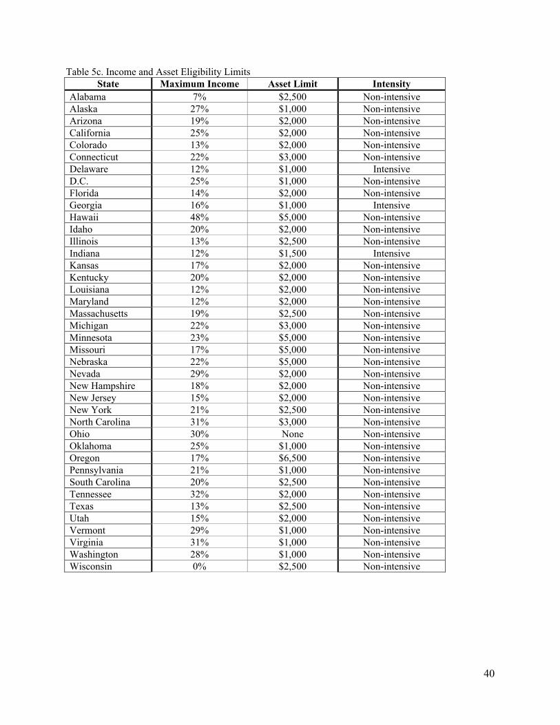
40

Table 5c. Income and Asset Eligibility Limits State Maximum Income Asset Limit Intensity

Alabama 7% $2,500 Non-intensive Alaska 27% $1,000 Non-intensive Arizona 19% $2,000 Non-intensive California 25% $2,000 Non-intensive Colorado 13% $2,000 Non-intensive Connecticut 22% $3,000 Non-intensive Delaware 12% $1,000 Intensive D.C. 25% $1,000 Non-intensive Florida 14% $2,000 Non-intensive Georgia 16% $1,000 Intensive Hawaii 48% $5,000 Non-intensive Idaho 20% $2,000 Non-intensive Illinois 13% $2,500 Non-intensive Indiana 12% $1,500 Intensive Kansas 17% $2,000 Non-intensive Kentucky 20% $2,000 Non-intensive Louisiana 12% $2,000 Non-intensive Maryland 12% $2,000 Non-intensive Massachusetts 19% $2,500 Non-intensive Michigan 22% $3,000 Non-intensive Minnesota 23% $5,000 Non-intensive Missouri 17% $5,000 Non-intensive Nebraska 22% $5,000 Non-intensive Nevada 29% $2,000 Non-intensive New Hampshire 18% $2,000 Non-intensive New Jersey 15% $2,000 Non-intensive New York 21% $2,500 Non-intensive North Carolina 31% $3,000 Non-intensive Ohio 30% None Non-intensive Oklahoma 25% $1,000 Non-intensive Oregon 17% $6,500 Non-intensive Pennsylvania 21% $1,000 Non-intensive South Carolina 20% $2,500 Non-intensive Tennessee 32% $2,000 Non-intensive Texas 13% $2,500 Non-intensive Utah 15% $2,000 Non-intensive Vermont 29% $1,000 Non-intensive Virginia 31% $1,000 Non-intensive Washington 28% $1,000 Non-intensive Wisconsin 0% $2,500 Non-intensive

41

Table 5d. Sanction and Diversion Policies State Sanction

Amount Sanction Length Diversion Intensity

Alabama Entire Benefit 6 months No Non-intensive Alaska Adult Portion 12 months Yes Intensive Arizona Entire Benefit 1 month No Non-intensive California Adult Portion 6 months No Non-intensive Colorado Entire Benefit 3 months Yes Intensive Connecticut Entire Benefit 3 months No Non-intensive Delaware Entire Benefit Permanent No Intensive D.C. Adult Portion 6 months No Non-intensive Florida Entire Benefit 3 months Yes Intensive Georgia Entire Benefit Permanent No Intensive Hawaii Adult Portion 6 months No Non-intensive Idaho Entire Benefit Permanent Yes Very Intensive Illinois Entire Benefit 3 months No Non-intensive Indiana Adult Portion 36 months No Non-intensive Kansas Entire Benefit 2 months No Non-intensive Kentucky Adult Portion Until Compliance Yes Non-intensive Louisiana Entire Benefit Until Compliance No Non-intensive Maryland Entire Benefit 1 month Yes Intensive Massachusetts Entire Benefit 1 month No Non-intensive Michigan Entire Benefit 1 month No Non-intensive Minnesota Adult Portion 1 month Yes Non-intensive Missouri Adult Portion 6 months No Non-intensive Nebraska Entire Benefit 12 months No Intensive Nevada Entire Benefit Permanent Yes Very Intensive New Hampshire Adult Portion 1 month No Non-intensive New Jersey Entire Benefit 3 months No Non-intensive New York Adult Portion 6 months No Non-intensive North Carolina Adult Portion 6 months Yes Non-intensive Ohio Entire Benefit 6 months Yes Intensive Oklahoma Adult Portion Until Compliance No Non-intensive Oregon Entire Benefit Until Compliance No Non-intensive Pennsylvania Adult Portion Permanent No Non-intensive South Carolina Entire Benefit 1 month No Non-intensive Tennessee Entire Benefit 3 months No Non-intensive Texas Adult Portion 6 months Yes Non-intensive Utah $100 Until Compliance Yes Non-intensive Vermont Adult Portion 6 months No Non-intensive Virginia Entire Benefit 6 months Yes Intensive Washington Adult Portion 1 month Yes Non-intensive Wisconsin Entire Benefit Permanent Yes Very Intensive

42

Table 5e. Lifetime Limits State Life Limit Intensity

Alabama 60 months+ Non-intensive Alaska 60 months+ Non-intensive Arizona 60 months+ Non-intensive California 60 months+ Non-intensive Colorado 60 months+ Non-intensive Connecticut 21 months Intensive Delaware 60 months+ Non-intensive D.C. 60 months+ Non-intensive Florida 48 months Intensive Georgia 48 months Intensive Hawaii 60 months+ Non-intensive Idaho 24 months Intensive Illinois 60 months+ Non-intensive Indiana 60 months+ Non-intensive Kansas 60 months+ Non-intensive Kentucky 60 months+ Non-intensive Louisiana 60 months+ Non-intensive Maryland 60 months+ Non-intensive Massachusetts 60 months+ Non-intensive Michigan 60 months+ Non-intensive Minnesota 60 months+ Non-intensive Missouri 60 months+ Non-intensive Nebraska 60 months+ Non-intensive Nevada 60 months+ Non-intensive New Hampshire 60 months+ Non-intensive New Jersey 60 months+ Non-intensive New York 60 months+ Non-intensive North Carolina 60 months+ Non-intensive Ohio 36 months Intensive Oklahoma 60 months+ Non-intensive Oregon 60 months+ Non-intensive Pennsylvania 60 months+ Non-intensive South Carolina 60 months+ Non-intensive Tennessee 60 months+ Non-intensive Texas 60 months+ Non-intensive Utah 36 months Intensive Vermont 60 months+ Non-intensive Virginia 60 months+ Non-intensive Washington 60 months+ Non-intensive Wisconsin 60 months+ Non-intensive

43

Changes in Marital Bargaining Power in Intensive and Non-intensive Reform States In the previous section I qualitatively characterized states as “intensive” reformers and

“non-intensive” reformers based on their welfare reform implementation policies. I use this variation in policy across states, along with variation over time, to precisely identify the effect of welfare reform on marital bargaining power. Intensive Reform States

I first estimate the differential change in the male bias for vulnerable women in intensive reform states over the period. In this set of regressions, we would expect to see positive and significant changes in the male bias if intensive welfare reform policies effectively reduced the marital bargaining power of lower-income married women with young children relative to other married women.

I limit my sample to observations from the 20 states characterized as intensive reformers. This sample includes 3,853 families headed by married couples. As shown in model (7), I regress male bias on the subgroup indicator, the post-period indicator, the interaction between subgroup and post-period, and a full set of controls. (7) Male Bias = β0 + δ0subgroup + β1post + δ1subgroup*post + βkXik + µ The coefficient of interest is δ1, the difference-in-differences estimator. This model is the same as the model used to estimate the differential change in the male bias over time, but in this case the sample is restricted to those states characterized as intensive reformers. Therefore, the interpretation of the coefficient δ1 is somewhat different. If the coefficient is positive and significant, we can conclude there is a differential change in the bargaining power of lower-income women with young children relative to other married women living in intensive reform states over the period. I find evidence of large and significant effects of welfare reform in states with intensive reform policies. I estimate an increase of 20.89 percentage points (p=.00) in the male bias for women with young children living in poverty, and 7.65 percentage points (p=.00) for low-income women. This estimate remains large and significant for income subgroups up to 500 percent of the poverty line. For the subgroup living at or below 500 percent of the poverty line, the estimated effect is a 3.55 percentage point (p=.04) increase in the male bias. Across subgroups we see similar relationships between male bias and the control variables as those presented in Table 4a. These results are presented in Table 6a.

44

Non-intensive Reform States

I then estimate the differential change in the male bias for lower-income women with young children relative to other married women living in non-intensive states over the same period. In this set of regressions, we would expect to see little change in the male bias because the policy treatment was relatively weak. While the safety net did not become stronger in these states, it did not become much weaker either. I limit my sample to observations from the 20 states characterized as non-intensive reformers. My sample includes 3,656 families headed by married couples. I use the same model as above, regressing male bias on the subgroup indicator, the post-period indicator, the interaction between subgroup and post-period, and a full set of controls. I find no evidence of a differential change in bargaining power of women with young children in non-intensive states. These results are presented in Table 6b. The findings from samples of intensive and non-intensive reform states support the theoretical prediction that intensive welfare reform policies reduced the marital bargaining power of those women most likely to perceive welfare as an alternative to marriage. We see large, significant effects of welfare reform in intensive reforms states and no evidence of effects in non-intensive reform states. Next, I isolate vulnerable subgroups of women and estimate the differential effect of welfare reform across states by the intensity of state reforms. Change in Marital Bargaining Power for Lower-income Women with Young Children across Intensive and Non-intensive Reform States

Finally, I restrict my sample to poor, married women with young children (348 families).

I then use model (8) to estimate the differential change in the male bias for those women who are living in intensive reform states relative to poor women with young children living in non-intensive reform states. (8) Male Bias = β0 + δ0intensive + β1post + δ1intensive*post + βkXik + µ I regress male bias on the intensive reform state indicator, the post-period indicator, the interaction between intensive reform and the post-period, and a full set of controls. I estimate a 17.44 percentage point (p=.01) increase in the male bias for poor women in intensive-reform states relative to their counterparts in non-intensive reform states over the period of welfare reform. I then expand my sample to include women in progressively higher income groups and use model (8) to determine the differential effect of living in an intensive reform state within each group. Therefore, the sample size grows with the increase in the income level of those women included in the sample. I find those women living at or below 200 percent of the poverty level experienced an estimated 7.90 percentage point (p=.04) increase in the male bias relative to their counterparts in non-intensive reform states. The effect remains positive, sizeable, and significant through women living at or below 300 percent of the poverty line. These results are presented in Table 6c.

45

Table 6a. Differential Change in the Male Bias for Lower-income Married Women with Young Children Living in Intensive Reform States (1995-2000) Percent of the Poverty Level: 100% 200% 300% 400% 500% Intercept -8.51** -8.25** -8.32** -8.77** -9.13** (3.28) (3.29) (3.30) (3.31) (3.30) Vulnerable Subgroup -10.84** -6.16** -4.11** -1.50 1.07 (2.43) (1.92) (1.74) (1.78) (1.94) Post Reform Period -0.39 -0.28 -0.59 -0.56 -0.43 (0.82) (0.84) (0.87) (0.90) (0.92) Subgroup*Post 20.89** 7.65** 6.49** 4.80** 3.55** (4.16) (2.61) (2.08) (1.87) (1.77) Percent of Poverty Line 1.37** 1.36** 1.39** 1.44** 1.48** (0.14) (0.14) (0.14) (0.14) (0.14) Young Children -7.04** -6.79** -7.05** -8.03** -9.63** (0.97) (1.03) (1.16) (1.35) (1.61) Family Size 0.32 0.30 0.32 0.33 0.34 (0.35) (0.35) (0.35) (0.35) (0.35) Husband: Age -0.04 -0.04 -0.04 -0.04 -0.04 (0.10) (0.10) (0.10) (0.10) (0.10) Wife: Age 0.03 0.01 0.02 0.03 0.03 (0.10) (0.10) (0.10) (0.10) (0.10) Husband: Black -3.25 -2.88 -2.67 -2.57 -2.55 (3.50) (3.51) (3.50) (3.51) (3.50) Wife: Black 0.69 0.53 0.25 0.10 0.10 (3.70) (3.71) (3.70) (3.71) (3.71) Husband: Asian 1.24 0.90 1.02 0.97 0.89 (2.85) (2.86) (2.86) (2.86) (2.88) Wife: Asian -3.60 -3.34 -3.43 -3.37 -3.26 (2.69) (2.69) (2.70) (2.70) (2.70) Husband: Hispanic -4.41** -4.33** -4.22** -4.24** -4.33** (1.93) (1.94) (1.94) (1.94) (1.94) Wife: Hispanic 1.32 1.33 1.12 1.08 1.17 (1.90) (1.91) (1.91) (1.91) (1.91) Husband: <HS 3.94** 4.14** 4.10** 4.12** 4.11** (2.01) (2.01) (2.01) (2.01) (2.01) Husband: HS 3.93** 3.84** 3.85** 3.78** 3.74** (1.55) (1.55) (1.55) (1.55) (1.55) Husband: SC 4.34** 4.23** 4.25** 4.24** 4.19** (1.49) (1.49) (1.49) (1.49) (1.49) Husband: BA 2.00 1.89 1.88 1.93 1.96 (1.42) (1.42) (1.42) (1.43) (1.42) Wife: <HS -2.58 -2.37 -2.55 -2.70 -2.75 (2.18) (2.19) (2.19) (2.19) (2.19) Wife: HS 1.80 1.97 2.01 1.94 1.82 (1.69) (1.69) (1.70) (1.70) (1.70) Wife: SC 0.84 0.96 0.98 0.92 0.87 (1.60) (1.60) (1.60) (1.60) (1.60) Wife: BA 0.11 0.22 0.25 0.29 0.23 (1.56) (1.56) (1.56) (1.56) (1.56) Large City -0.17 -0.27 -0.31 -0.31 -0.33 (1.29) (1.29) (1.29) (1.29) (1.29) Small City 5.28** 5.21** 5.18** 5.15** 5.11** (1.38) (1.38) (1.38) (1.38) (1.38) R2 0.08 0.08 0.08 0.08 0.08 N 3,853 3,853 3,853 3,853 3,853 * significant at p < .10; ** significant at p < .05

46

Table 6b. Differential Change in the Male Bias for Lower-income Married Women with Young Children Living in Non-intensive Reform States (1995-2000) Percent of the Poverty Level: 100% 200% 300% 400% 500% Intercept -0.69 1.12 0.67 0.23 -0.28 (3.49) (3.51) (3.51) (3.52) (3.52) Vulnerable Subgroup -10.47** -6.00** -3.89** -1.81 0.44 (2.54) (1.99) (1.82) (1.91) (2.18) Post Reform Period 0.67 0.87 0.64 0.57 0.60 (0.86) (0.89) (0.92) (0.95) (0.98) Subgroup*Post 1.16 -0.41 0.70 0.96 0.76 (3.83) (2.67) (2.20) (1.99) (1.87) Percent of Poverty Line 1.62** 1.64** 1.69** 1.75** 1.82** (0.16) (0.16) (0.16) (0.17) (0.17) Young Children -4.59** -4.25** -4.34** -5.17** -6.69** (1.06) (1.13) (1.27) (1.50) (1.87) Family Size -1.38** -1.32** -1.32** -1.32** -1.30** (0.37) (0.37) (0.37) (0.37) (0.37) Husband: Age -0.11 -0.14 -0.14 -0.14 -0.14 (0.11) (0.11) (0.11) (0.11) (0.11) Wife: Age 0.12 0.13 0.13 0.14 0.14 (0.11) (0.11) (0.11) (0.11) (0.11) Husband: Black -2.35 -2.61 -2.35 -2.36 -2.36 (4.81) (4.82) (4.83) (4.83) (4.83) Wife: Black -4.63 -4.40 -4.60 -4.58 -4.55 (4.89) (4.90) (4.90) (4.91) (4.91) Husband: Asian -4.62 -4.80 -4.81 -4.78 -4.69 (4.36) (4.37) (4.37) (4.38) (4.38) Wife: Asian -5.99 -5.82 -5.86 -5.88 -5.96 (4.05) (4.05) (4.06) (4.06) (4.06) Husband: Hispanic 1.20 1.02 0.81 0.76 0.70 (2.45) (2.45) (2.46) (2.46) (2.46) Wife: Hispanic -3.42 -2.89 -2.94 -3.08 -3.08 (2.33) (2.33) (2.33) (2.33) (2.33) Husband: <HS 8.73** 9.05** 9.07** 9.00** 9.01** (2.21) (2.21) (2.22) (2.22) (2.22) Husband: HS 9.30** 9.40** 9.52** 9.49** 9.50** (1.73) (1.73) (1.73) (1.73) (1.73) Husband: SC 8.09** 8.25** 8.40** 8.45** 8.44** (1.66) (1.66) (1.66) (1.66) (1.66) Husband: BA 5.23** 5.25** 5.36** 5.48** 5.54** (1.59) (1.60) (1.60) (1.60) (1.60) Wife: <HS -3.32 -3.30 -3.34 -3.40 -3.46 (2.27) (2.27) (2.27) (2.28) (2.28) Wife: HS -0.19 0.08 0.11 0.04 -0.07 (1.82) (1.82) (1.83) (1.83) (1.83) Wife: SC 1.39 1.52 1.70 1.63 1.57 (1.75) (1.75) (1.76) (1.76) (1.76) Wife: BA -1.04 -1.06 -0.96 -0.93 -0.93 (1.72) (1.72) (1.73) (1.73) (1.73) Large City -5.42** -5.77** -5.63** -5.64** -5.62** (1.35) (1.35) (1.35) (1.35) (1.35) Small City -2.09 -2.36* -2.17 -2.15 -2.15 (1.43) (1.44) (1.44) (1.44) (1.44) R2 0.11 0.11 0.10 0.10 0.10 N 3,656 3,656 3,656 3,656 3,656 * significant at p < .10; ** significant at p < .05

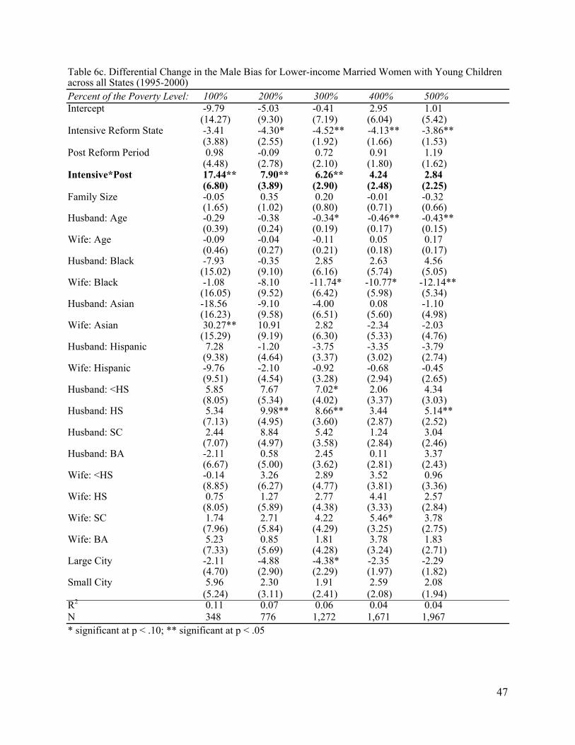
47

Table 6c. Differential Change in the Male Bias for Lower-income Married Women with Young Children across all States (1995-2000) Percent of the Poverty Level: 100% 200% 300% 400% 500% Intercept -9.79 -5.03 -0.41 2.95 1.01 (14.27) (9.30) (7.19) (6.04) (5.42) Intensive Reform State -3.41 -4.30* -4.52** -4.13** -3.86** (3.88) (2.55) (1.92) (1.66) (1.53) Post Reform Period 0.98 -0.09 0.72 0.91 1.19 (4.48) (2.78) (2.10) (1.80) (1.62) Intensive*Post 17.44** 7.90** 6.26** 4.24 2.84 (6.80) (3.89) (2.90) (2.48) (2.25) Family Size -0.05 0.35 0.20 -0.01 -0.32 (1.65) (1.02) (0.80) (0.71) (0.66) Husband: Age -0.29 -0.38 -0.34* -0.46** -0.43** (0.39) (0.24) (0.19) (0.17) (0.15) Wife: Age -0.09 -0.04 -0.11 0.05 0.17 (0.46) (0.27) (0.21) (0.18) (0.17) Husband: Black -7.93 -0.35 2.85 2.63 4.56 (15.02) (9.10) (6.16) (5.74) (5.05) Wife: Black -1.08 -8.10 -11.74* -10.77* -12.14** (16.05) (9.52) (6.42) (5.98) (5.34) Husband: Asian -18.56 -9.10 -4.00 0.08 -1.10 (16.23) (9.58) (6.51) (5.60) (4.98) Wife: Asian 30.27** 10.91 2.82 -2.34 -2.03 (15.29) (9.19) (6.30) (5.33) (4.76) Husband: Hispanic 7.28 -1.20 -3.75 -3.35 -3.79 (9.38) (4.64) (3.37) (3.02) (2.74) Wife: Hispanic -9.76 -2.10 -0.92 -0.68 -0.45 (9.51) (4.54) (3.28) (2.94) (2.65) Husband: <HS 5.85 7.67 7.02* 2.06 4.34 (8.05) (5.34) (4.02) (3.37) (3.03) Husband: HS 5.34 9.98** 8.66** 3.44 5.14** (7.13) (4.95) (3.60) (2.87) (2.52) Husband: SC 2.44 8.84 5.42 1.24 3.04 (7.07) (4.97) (3.58) (2.84) (2.46) Husband: BA -2.11 0.58 2.45 0.11 3.37 (6.67) (5.00) (3.62) (2.81) (2.43) Wife: <HS -0.14 3.26 2.89 3.52 0.96 (8.85) (6.27) (4.77) (3.81) (3.36) Wife: HS 0.75 1.27 2.77 4.41 2.57 (8.05) (5.89) (4.38) (3.33) (2.84) Wife: SC 1.74 2.71 4.22 5.46* 3.78 (7.96) (5.84) (4.29) (3.25) (2.75) Wife: BA 5.23 0.85 1.81 3.78 1.83 (7.33) (5.69) (4.28) (3.24) (2.71) Large City -2.11 -4.88 -4.38* -2.35 -2.29 (4.70) (2.90) (2.29) (1.97) (1.82) Small City 5.96 2.30 1.91 2.59 2.08 (5.24) (3.11) (2.41) (2.08) (1.94) R2 0.11 0.07 0.06 0.04 0.04 N 348 776 1,272 1,671 1,967 * significant at p < .10; ** significant at p < .05

48

Change in Marital Bargaining Power for Lower-income Women with Young Children Living in Intensive Reform States over the Period of Welfare Reform

I then return to the full sample of families headed by married couples, excluding those states for which data or identifiers were not available (7,509 families). My final model estimates the differential change in male bias for lower-income women with young children living in intensive reform states over the period of welfare reform.

Using model (9), I regress male bias on the subgroup indicator, the intensive reform state

indicator, the post-period indicator, the two-way interactions between these three variables, the three-way interaction between these variables, and a full set of controls. (9) Male Bias = β0 + δ0subgroup + β1intensive + β2post + δ1subgroup*post + δ2post*intensive + δ3post*subgroup + δ4subgroup*intensive*post + βkXik + µ In this final analysis, the coefficient on the three-way interaction term (δ4) represents the triple-difference estimator, which captures the differential change in the male bias for lower-income women with young children in states that enacted the more intensive policy reforms over the period. Table 7 presents these results.

I find evidence of large and significant differential changes in the bargaining power of vulnerable women in intensive-reform states. Poor women with young children in intensive reform states experience an estimated 20.0 percentage point (p=.00) increase in the male bias relative to other married women. Those women in the subgroup living at or below 200 percent of the poverty level experience an estimated 8.47 percentage point (p=.02) differential increase in the male bias. The effect of intensive welfare reform on the male bias remains positive, sizable, and significant for women living at or below 300 percent of the poverty line. Estimates remain positive, but are not significant, for relatively higher-income subgroups of women through 500 percent of the poverty line. Coefficient estimates on the control characteristics are consistent with earlier findings.

49

Table 7. Differential Change in the Male Bias for Married Women with Young Children over Time and across States (1995-2000) Percent of the Poverty Level: 100% 200% 300% 400% 500% Intercept -2.27 -1.99 -2.28 -2.75 -3.20 (2.43) (2.44) (2.45) (2.46) (2.46) Vulnerable Subgroup -10.47** -5.65** -3.49** -1.28 1.08 (2.43) (1.85) (1.61) (1.59) (1.70) Intensive Reform State -3.21** -3.18** -3.09** -3.07** -3.05** (0.80) (0.83) (0.86) (0.89) (0.92) Post Reform Period 0.47 0.66 0.45 0.40 0.43 (0.84) (0.86) (0.90) (0.93) (0.95) Subgroup*Post 0.89 -0.56 0.69 0.90 0.74 (3.76) (2.63) (2.16) (1.95) (1.84) Post*Intensive -0.64 -0.76 -0.89 -0.83 -0.76 (1.15) (1.19) (1.24) (1.28) (1.31) Subgroup*Intensive -0.56 -0.80 -1.07 -0.83 -0.71 (3.34) (2.47) (2.03) (1.84) (1.76) Subgroup*Intensive*Post 19.99** 8.47** 6.08** 4.16 3.12 (5.66) (3.73) (3.02) (2.72) (2.57) Percent of Poverty Line 1.48** 1.49** 1.53** 1.58** 1.63** (0.10) (0.11) (0.11) (0.11) (0.11) Young Children -5.84** -5.58** -5.76** -6.65** -8.24** (0.72) (0.76) (0.86) (1.00) (1.22) Family Size -0.52** -0.50 -0.49* -0.48* -0.47* (0.26) (0.26) (0.26) (0.26) (0.26) Husband: Age -0.07 -0.08 -0.08 -0.09 -0.08 (0.07) (0.07) (0.07) (0.07) (0.07) Wife: Age 0.07 0.07 0.07 0.07 0.08 (0.07) (0.07) (0.07) (0.07) (0.07) Husband: Black -2.97 -2.84 -2.62 -2.56 -2.56 (2.85) (2.85) (2.85) (2.85) (2.85) Wife: Black -2.04 -2.08 -2.30 -2.39 -2.36 (2.95) (2.96) (2.96) (2.96) (2.96) Husband: Asian -0.91 -1.22 -1.14 -1.17 -1.21 (2.40) (2.41) (2.41) (2.41) (2.41) Wife: Asian -4.48** -4.24* -4.31* -4.28* -4.22* (2.25) (2.26) (2.26) (2.26) (2.26) Husband: Hispanic -2.66* -2.69* -2.71* -2.76* -2.83* (1.52) (1.52) (1.53) (1.53) (1.53) Wife: Hispanic -0.68 -0.45 -0.59 -0.66 -0.61 (1.48) (1.48) (1.48) (1.48) (1.48) Husband: <HS 6.15** 6.41** 6.41** 6.39** 6.40** (1.49) (1.49) (1.49) (1.49) (1.49) Husband: HS 6.43** 6.43** 6.50** 6.46** 6.44** (1.15) (1.16) (1.16) (1.16) (1.16) Husband: SC 6.02** 6.04** 6.13** 6.15** 6.14** (1.11) (1.11) (1.11) (1.11) (1.11) Husband: BA 3.38** 3.32** 3.38** 3.46** 3.52** (1.06) (1.06) (1.07) (1.07) (1.07) Wife: <HS -2.50 -2.40 -2.50 -2.60* -2.66* (1.57) (1.57) (1.58) (1.58) (1.58) Wife: HS 1.07 1.30 1.34 1.28 1.17 (1.24) (1.24) (1.24) (1.25) (1.25) Wife: SC 1.41 1.54 1.64 1.60 1.54 (1.18) (1.18) (1.18) (1.19) (1.19) Wife: BA -0.23 -0.18 -0.11 -0.07 -0.10 (1.16) (1.16) (1.16) (1.16) (1.16) Large City -2.87** -3.07** -3.04** -3.04** -3.05** (0.93) (0.93) (0.93) (0.93) (0.93) Small City 1.65* 1.51 1.57 1.56 1.53 (0.99) (0.99) (0.99) (0.99) (0.99) R2 0.09 0.09 0.09 0.09 0.09 N 7,509 7,509 7,509 7,509 7,509 * significant at p < .10; ** significant at p < .05

50

Summary of Findings In my analysis of the causal impact of welfare reform on male bias, I first use the time

period over which welfare reform was implemented at the national level to estimate the differential change in the bargaining power of married women with young children relative to all other married families. For poor women, I estimate a differential and significant increase of 10.6 percentage points in the male bias over the period. This effect persists and remains significant for relatively higher-income groups of women.

To precisely identify the effect of welfare reform, I then use variation in policy

implementation across states over the period of reform. Based on qualitative characterizations of states as “intensive” reformers or “non-intensive” reformers, I limit my sample to allow for estimation of two-way interaction effects. I first restrict the sample to intensive reform states and estimate a differential and significant increase of 20.9 percentage points in the male bias for poor women with young children. This effect persists and remains significant for relatively higher-income groups of women. I then restrict my sample to non-intensive reform states and find no evidence of a differential change in bargaining power over the period. Finally, I restrict my sample to subgroups of lower-income women across all states. I estimate a differential and significant increase in the male bias of 17.4 percentage points for poor women. This estimate remains positive, sizable, and significant for women living at or below 300 percent of the poverty line.

In the final stage of my analysis, I return to the full sample of married couples and

estimate the differential change in the bargaining power of lower-income women with young children in intensive-reform states over the period of welfare reform. I estimate large, significant effects of welfare reform on male bias. I estimate a differential and significant increase in the male bias of 20.0 percentage points for poor women; 8.5 percentage points for women living at or below 200 percent of the poverty level; and 6.1percentage points for women living at or below 300 percent of the poverty level. Estimates for changes in the male bias for relatively higher-income women remain positive through 500 percent of the poverty level, but are not significant. Based on these findings, I conclude that the weakening of the social safety net through welfare reform reduced the marital bargaining power of poor and low-income women, those most likely to consider welfare as a possible exit alternative to their marriages.

51

VI. Policy Implications

Findings from this study show that welfare reform substantially reduced the marital bargaining power of poor and low-income women with young children. These findings have narrow implications for evaluating welfare reform and broad implications for how we design and implement future policies that may impact the allocation of resources within families. Implications for Evaluating Welfare Reform

The goal of welfare reform was to address the perverse work, marriage, and childbearing incentives experienced by the welfare recipient population. On average, recipient and would-be recipient families may have experienced benefits from welfare reform to the extent that work, marriage, and childbearing decisions were influenced by changes in these incentives. Based on impact studies, it appears some families did benefit through higher incomes and increased family stability, while others experienced increased economic hardship (Ellwood 2000; Loprest 2001; Blank 2002; Danziger et al. 2002; Johnson, Kalil, and Dunifon 2007). However, welfare reform had impacts beyond the recipient population. There is some debate over the extent to which welfare reform actually reduced budgetary costs. The average spending level in the four years following the implementation of welfare reform was lower than the average spending level in the four years prior to reform. However, economic conditions also improved substantially during the post-reform years, suggesting budgetary costs would have declined even in the absence of reform (Figlio et al. 2000), and the observed decline in spending over the period was roughly proportional to the decline in caseloads (Scholz, Moffitt, and Cowan 2009). While transferring benefits from would-be recipients back to taxpayers does not represent a gain to society overall, those reductions in budgetary costs associated with efficiency gains through program reform should be counted as benefits associated with the legislation. We now understand that an evaluation of welfare reform that stops at this point has left out an important population. The presumed gains associated with welfare reform were primarily achieved through restrictions in the social safety net for poor women and their children, resulting in losses in marital bargaining power for non-recipient, low-income mothers. While indirect, the effect of welfare reform was to induce a shift in intra-family resource allocation. Given the correlation between women’s bargaining power and children’s consumption levels in the literature, these findings suggest welfare reform led to a reduction in allocations toward children (Thomas 1990; Lundberg, Pollak, and Wales 1997; Phipps and Burton 1998; Duflo 2003; Rangel 2006; Bobonis 2009). A complete evaluation of welfare reform would need to weigh the presumed benefits to recipients and taxpayers against these costs to married women and children in low-income families.

52

Implications for Future Policy

Three of the four stated goals of PRWORA focus on traditional family formation. Welfare reform policies aim to increase marriage, decrease non-marital childbearing, and increase the proportion of children raised in two-parent families. The primary mechanism through which these goals were to be achieved was the restriction of the social safety net, leaving mothers more dependent on men for economic survival. The secondary consequence of taking this approach to achieving family formation goals was to effectively reduce the consumption of low-income married women and children. Numerous public supports are intended to increase the well-being of children in low-income families. The findings in this study build on a literature that suggests policies that increase mothers’ ownership of family income or improve mothers’ relative positions in divorce may induce increases in children’s consumption and well-being. To the extent that we are concerned with principal-agent problems or under-allocation problems of any kind in low-income families, these findings have important efficiency implications. Welfare reform is just one example of a policy change that may indirectly affect the intra-family allocation of resources. Any policy that impacts the ownership of income within marriage or the relative well-being of partners in divorce may affect the relative bargaining power of husbands and wives. To the extent that we continue to perceive families as single utility-maximizing units, we miss the equity implications of many policy proposals. Policies that have the potential to improve the well-being of families overall may have differential impacts on individuals within families. The distribution of these impacts needs to be fully considered.

53

References Bachu, Amara. 1999. “Trends in premarital childbearing: 1930 to 1994, Current Population Reports.” Washington: Census Bureau. Becker, Gary. 1974. “A Theory of Marriage: Part II.” The Journal of Political Economy 82(2):S11-S26. Becker, Gary, Elizabeth Landes, and Robert Michael. 1977. “An Economic Analysis of Marital Instability.” Journal of Political Economy 85(6):1141-87. Becker, Gary. 1981. A Treatise on the Family. Cambridge, MA: Harvard University Press. Bell, Winifred. 1965. Aid to Families with Dependent Children. New York: Columbia University Press. Bertrand, Marianne, Esther Duflo, and Sendhil Mullainathan. 2004. “How Much Should We Trust Differences-in-Differences Estimates?” Quarterly Journal of Economics 119(1):249-75. Bitler, Marianna, Jonah Gelbach, Hilary Hoynes, and Madeline Zavodny. 2004. “The Impact of Welfare Reform on Marriage and Divorce” Demography 41(2): 213-236. Blank, Rebecca. 2002. “Evaluating Welfare Reform in the United States,” Journal of Economic Literature 40(4). Bobonis, Gustavo. 2009. “Is the Allocation of Resources within the Household Efficient? New Evidence from a Randomized Experiment.” Journal of Political Economy 117(3):453-503. Browning, Martin, François Bourguignon, Pierre-André Chiappori, Valérie Lechene. 1994. “Incomes and Outcomes: A Structural Model of Intrahousehold Allocation.” Journal of Political Economy 102(6):1067-1096. Chase-Lansdale, Lindsay, and Maris Vinovskis. 1997. “Whose Responsibility? An Historical Analysis of the Changing Roles of Mothers, Fathers, and Society.” In Escape from Poverty: What Makes a Difference for Children? Lindsay Chase-Lansdale and Jeanne Brooks-Gunn, eds. Cambridge: Cambridge University Press. Chiappori, Pierre-André, Bernard Fortin, and Guy Lacroix. 2002. “Marriage Market, Divorce Legislation, and Household Labor Supply.” The Journal of Political Economy 110(1):37-72. Danziger, Sheldon, Colleen Heflin, Mary Corcoran, Elizabeth Otlmans, and Hue-Chen Wang. 2002. “Does It Pay to Move from Welfare to Work?” Journal of the Association for Policy Analysis and Management 21(4): 671-692. Duflo, Esther. 2003. “Grandmothers and Granddaughters: Old Age Pension and Intrahousehold Allocation in South Africa.” The World Bank Economic Review 17(1):1-25.

54

Edin, Kathryn. 2000. “What Do Low-Income Single Mothers Say about Marriage?” Social Problems 47(1):112-133. Ellwood, David. 2000. “The Impact of the Earned Income Tax Credit and Social Policy Reforms on Work, Marriage, and Living Arrangements.” National Tax Journal 53(4.2):1063-1105. Figlio, David and James Ziliak. 1999. “Welfare Reform, the Business Cycle, and the Decline in AFDC Caseloads,” in Economic Conditions and Welfare Reform. Sheldon Danziger, ed. Kalamazoo, MI: W.E. Upjohn Institute for Employment Research. Goldin, Claudia, and Lawrence Katz. 2002. “The Power of the Pill.” Journal of Political Economy 110:730–770. Goldberg v. Kelly, 397 U.S. 254 (1970) Goodwin, Joanna. 1995. “Employable Mothers and Suitable Work: A Re-Evaluation of Welfare and Wage-Earning for Women in the Twentieth-Century United States.” Journal of Social History 29(2):253-274. Gordon, Linda. 1994. Pitied, but not Entitled. New York: Free Press. Gray, Jeffrey. 1998. “Divorce-Law Changes, Household Bargaining, and Married Women’s Labor Supply.” American Economic Review 88(3):628–642. Handler, Joel. 1972. Reforming the Poor: Welfare Policy, Federalism, and Morality. New York: Basic Books. Holcomb, Pamela. 1993. Welfare Reform: The Family Support Act in Historical Context. Washington, DC: Urban Institute. Johnson, Rucker, Ariel Kalil, and Rachel Dunifon. 2010. Mothers’ Work and Children’s Lives: Low-income Families After Welfare Reform. Kalamazoo, MI: Upjohn Institute Press. King v. Smith, 392 U.S. 309 392 (1968) Klawon, Emily, and Jill Tiefenthaler. 2001. “Bargaining over Family Size: The Determinants of Fertility in Brazil.” Population Research and Policy Review 20(5):423-440. Lundberg, Shelly, Robert Pollak, Terence Wales. 1997. “Do Husbands and Wives Pool Their Resources? Evidence from the United Kingdom Child Benefit.” The Journal of Human Resources 32(3):463-480.

55

Loprest, Pamela. 2001. How Are Families that Left Welfare Doing? A Comparison of Early and Recent Welfare Leavers. Series B, No B-36, Assessing the New Federalism Project. Washington, D.C.: Urban Institute. Manser, Marilyn, and Murray Brown. 1980. “Marriage and Household Decision-Marking: A Bargaining Analysis.” International Economic Review 21(1):31-44. Mink, Gwendolyn. 1995. The Wages of Motherhood: Inequality in the Welfare State. Ithaca: Cornell University Press. McElroy, Marjorie, and Mary Jean Horney. 1981. “Nash-Bargained Household Decisions: Toward a Generalization of the Theory of Demand.” International Economic Review 22(2): 333-349. Nightingale, Demetra Smith, and Pamela Holcomb. 1997. “Alternative Strategies for Increasing Employment.” The Future of Children 7(1):52-64. Nightingale, Demetra Smith. 1997. “Work-related Resources and Services: Implications for TANF.” Washington: Urban Institute. Phipps, Shelly, and Peter Burton. 1996. “Collective Models of Family Behaviour: Implications for Economic Policy.” Canadian Public Policy 22(2):129-143. Phipps, Shelly, and Peter Burton. 1998. “What's Mine is Yours? The Influence of Male and Female Incomes on Patterns of Household Expenditure.” Economica 65(260):599-613. Rangel, Marcus. 2006. “Alimony Rights and Intrahousehold Allocation of Resources: Evidence from Brazil.” The Economic Journal, 116: 627–658. Rein, Mildred. 1982. “Work in Welfare: Past Failures and Future Strategies.” Social Science Review 56(2):211-229. Samuelson, Paul. 1956. “Social Indifference Curves.” The Quarterly Journal of Economics 70(1):1-22. Schultz, Paul. 1990. “Testing the Neoclassical Model of Family Labor Supply and Fertility.” The Journal of Human Resources 25(4):599-634. Scholz, John Karl, Robert Moffitt, and Benjamin Cowan. 2009. “Trends in Income Support,” in Changing Poverty, Changing Policies. Sheldon Danziger and Mary Cancian eds. Cambridge: Harvard University Press. Shapiro v. Thompson 394 US 618 (1969) Thomas, Duncan. 1990. “Intra-Household Resource Allocation: An Inferential Approach.” The Journal of Human Resources 25(4):635-664.