the effect of state taxes on the … systematic evidence on their effects is available. as noted in...
TRANSCRIPT

NBER WORKING PAPER SERIES
THE EFFECT OF STATE TAXES ON THE GEOGRAPHICAL LOCATION OF TOP EARNERS:EVIDENCE FROM STAR SCIENTISTS
Enrico MorettiDaniel Wilson
Working Paper 21120http://www.nber.org/papers/w21120
NATIONAL BUREAU OF ECONOMIC RESEARCH1050 Massachusetts Avenue
Cambridge, MA 02138April 2015
We are thankful for very helpful comments received from seminar participants at and Barcelona GSE,Berkeley, Federal Reserve Bank of San Francisco, IZA, National Tax Association, University of Hawaiiand from discussions by Jorge De La Roca and Juan Carlos Suárez Serrato. Yifan Cao provided excellentresearch assistance. Moretti gratefully acknowledges financial support from Microsoft. The viewsexpressed in the paper represent those of the authors and do not necessarily represent the views ofthe Federal Reserve Bank of San Francisco, the Federal Reserve System, or the National Bureau ofEconomic Research.
NBER working papers are circulated for discussion and comment purposes. They have not been peer-reviewed or been subject to the review by the NBER Board of Directors that accompanies officialNBER publications.
© 2015 by Enrico Moretti and Daniel Wilson. All rights reserved. Short sections of text, not to exceedtwo paragraphs, may be quoted without explicit permission provided that full credit, including © notice,is given to the source.

The Effect of State Taxes on the Geographical Location of Top Earners: Evidence from StarScientistsEnrico Moretti and Daniel WilsonNBER Working Paper No. 21120April 2015JEL No. H71,J01,J08,J18,J23,R0
ABSTRACT
Using data on the universe of U.S. patents filed between 1976 and 2010, we quantify how sensitiveis migration by star scientist to changes in personal and business tax differentials across states. Weuncover large, stable, and precisely estimated effects of personal and corporate taxes on star scientists’migration patterns. The long run elasticity of mobility relative to taxes is 1.6 for personal income taxes,2.3 for state corporate income tax and -2.6 for the investment tax credit. The effect on mobility is smallin the short run, and tends to grow over time. We find no evidence of pre-trends: Changes in mobilityfollow changes in taxes and do not to precede them. Consistent with their high income, star scientistsmigratory flows are sensitive to changes in the 99th percentile marginal tax rate, but are insensitiveto changes in taxes for the median income. As expected, the effect of corporate income taxes is concentratedamong private sector inventors: no effect is found on academic and government researchers. Moreover,corporate taxes only matter in states where the wage bill enters the state’s formula for apportioningmulti-state income. No effect is found in states that apportion income based only on sales (in whichcase labor’s location has little or no effect on the tax bill). We also find no evidence that changes instate taxes are correlated with changes in the fortunes of local firms in the innovation sector in theyears leading up to the tax change. Overall, we conclude that state taxes have significant effect of thegeographical location of star scientists and possibly other highly skilled workers. While there are manyother factors that drive when innovative individual and innovative companies decide to locate, thereare enough firms and workers on the margin that relative taxes matter.
Enrico MorettiUniversity of California, BerkeleyDepartment of Economics549 Evans HallBerkeley, CA 94720-3880and [email protected]
Daniel WilsonFederal Reserve Bank of San Francisco101 Market St.Mail Stop 1130San Francisco, CA [email protected]

2
1. Introduction
In the United States, personal taxes vary enormously from state to state. These geographical
differences are particularly large for high income taxpayers. Figure 1 shows differences across
states in the individual income marginal tax rate (MTR) for someone with income at the 99th
percentile nationally in 2010. The MTRs in California, Oregon, and Maine were 9.5%, 10.48%,
and 8.5%, respectively. By contrast, Washington, Texas, Florida, and six other states had a MTR
of zero. Large differences are also observed in business taxes. As shown in Figure 2, Iowa,
Pennsylvania, and Minnesota had corporate income taxes rates of 12%, 9.99%, and 9.8%,
respectively, while Washington, Nevada, and three other states had no corporate tax at all. And
not only do tax rates vary substantially across states, they also vary within states over time.
Figures 3, for instance, shows how states’ individual income MTRs changed during various
intervals spanning 1977 to 2010. Corporate tax rates exhibit similar within-state variation (see
Figure 4).
If workers and firms are mobile across state borders, these large differences over time and
place have the potential to significantly affect the geographical localization of highly skilled
workers and employers. The literature on the effect of taxes on the labor market has largely
focused on how taxes affect labor supply, and by enlarge it has ignored how taxes might affect the
geographical location of workers and firms. This is surprising because the effect of state taxes on
the ability of states to attract firms and jobs figures prominently in the policy debate in the U.S.
Many states aggressively and openly compete for firms and high skill workers by offering
low taxes. Indeed, low-tax states routinely advertise their favorable tax environments with the
explicit goal to attract households and business to their jurisdiction. Between 2012 and 2014,
Texas ran TV ads in California, Illinois and New York urging businesses and taxpayers to
relocate. Governor Rick Perry visited dozens of California companies to pitch Texas’ low taxes,
famously declaring: “Texas rewards success with no state income tax.” Similarly, Kansas has paid
for billboards in Midwestern states to advertise its recent tax cuts. Wisconsin Governor Scott
Walker has called upon Illinois and Minnesota employers to “escape to Wisconsin.” Louisiana
and Indiana have followed similar strategies. In the 2014 election cycle, state taxes and their
effect on local jobs were a prominent issue in many gubernatorial races.
But despite all the attention from policy makers and voters, the effect of taxes on the
geographical location of high earners and businesses remains poorly understood because little

3
systematic evidence on their effects is available. As noted in a recent paper by Kleven, Landais
and Saez (2013) there is “very little empirical work on the effect of taxation on the spatial
mobility of individuals, especially among high-skilled workers”.
In this paper, we seek to quantify how sensitive is internal migration by high-skilled workers
to personal and business tax differentials across U.S. states. Personal taxes might shift the supply
of workers to a state: states with high personal taxes presumably experience a lower supply of
workers for given before-tax average wage, cost of living and local amenities. Business taxes
might shift the demand for skilled workers by businesses: states with high business taxes
presumably experience a lower demand for workers, all else equal.
We focus on the locational decisions of star scientists, defined as scientists – in the private
sector as well as academia and government – with patent counts in the top 5% of the distribution.
Using data on the universe of U.S. patents filed between 1976 and 2010, we identify their state of
residence in each year. We compute bilateral migration flows for every pair of states (50x50) for
every year. We then relate bilateral out-migration to the differential between the destination and
origin state in personal and business taxes in each year. To this end, we compiled a
comprehensive data set on state personal income tax rates for taxpayers at the 99.9th, 99th, 95th,
50th percentiles of the income distribution; the state-level corporate income tax rate; the R&D tax
credit rate; and the investment tax credit rate.
Star scientists are important for at least two reasons. First, star scientists earn high incomes –
most of them are likely to be in the top 1% of the income distribution. By definition, star
scientists are exceptionally talented workers. By studying them, we hope to shed some light on
the locational decisions of other well-educated, highly productive and high income workers.
Second, and more fundamentally, star scientists are an important group of workers because their
locational decisions have potentially large consequences for local job creation. Unlike
professional athletes, movie stars and rich heirs – the focus of some previous research – the
presence of start scientists in a state is typically associated with research and production facilities
and in some cases, with entire industries, from biotech to software to nano-tech.1
1 The literature has highlighted the role that stars scientists have historically played in the birth and localization of new R&D-intensive industries. For example, the initial location of star scientists played a key role in determining the localization of the three main biotech clusters in the US (Zucker, Darby and Brewer, 1998). Similar patterns have been documented for semiconductors, computer science and nano-tech (Zucker and Darby, 2006).

4
Of course, taxes are not the only factor that determines the location of star scientists. Indeed,
we find no cross-sectional relationship between state taxes and number of star scientists as the
effect is swamped by all the other differences across states. California, for example, has relatively
high taxes throughout our sample period, but it is also attractive to scientists because the historical
presence of innovation clusters like Silicon Valley and the San Diego biotech cluster. Indeed,
California does not lose stars to Texas, even though Texas has no personal income tax and a low
business tax rate.
For this reason, our baseline model estimates the elasticity of migration to taxes using a
specification where the number of scientists who move from one state to another is a function of
the tax difference between the two states, conditional on state-pair ordered fixed effects. By using
changes over time to identify the effect of taxes, our models absorb all time-invariant factors that
can shift the demand of scientists and the supply of scientists across state pairs. Our models also
control for time-varying regional shocks by including region-of-origin*region-of-destination*year
dummies; and in some cases, state-of-origin*year dummies or state-of-destination*year dummies.
We uncover large, stable, and precisely estimated effects of personal and corporate taxes on
star scientists’ migration patterns. The probability of moving from state o (origin) to state d
(destination) increases when the tax rate differential between o and d increases. For taxpayers
with income at the 99th percentile of their state, we find a long-run elasticity of about 1.7: a 1%
decline in after-tax income in state d relative to state o driven by a change in the MTR for the top
1% of income earners is associated with a 1.7 percent increase in the number of star scientists
who leave state o and relocate in state d in the long-run. As an illustration, our estimates imply
that the effect of New York cutting its marginal tax rate on the top 1% of earners from 7.5% to
6.85% in 2006 was 12 fewer star scientists moving away and 12 more stars moving into New
York, for a net increase of 24 stars, a 2.1% increase.
While economically large, our estimates do not appear to be unrealistic when compared with
existing studies. Kleven, Landais, Saez and Schultz (2014) estimate a similar elasticity for
international migration of skilled workers in Europe. One might have expected our elasticity to be
larger, because it is presumably easier to relocate within a country that across countries.
We find a similar elasticity for state corporate income tax as well as the investment tax credit
(in the opposite direction), while the elasticity for the R&D credit rate is smaller and statistically

5
insignificant in some specifications. In all, our estimates suggest that both the supply of, and the
demand for, star scientists are highly sensitive to state taxes.
We can’t completely rule out the possibility that our estimates are biased by the presence of
unobserved shocks to demand or supply of scientists, but the weight of the available evidence
lends credibility to our estimates. First, when we focus on the timing of the effects, we find no
evidence of pre-trends: Changes in mobility follow changes in taxes and do not to precede them.
The effect on mobility is small in the short-run, and tends to grow over time, presumably because
it takes time for firms and workers to relocate.
Second, we find no evidence that changes in state taxes are correlated with changes in the
fortunes of local firms in the innovation sector in the years leading up to the tax change,
suggesting that states do not strategically change taxes to help local patenters at times when they
are struggling (or thriving). In particular, when we regress changes in state taxes on lagged
changes in the market value of the top five patenting companies in the state, we find no
relationship.
It is still possible that there are changes in economic policies other than taxes that could be
correlated with taxes. For example, a pro-business state legislature could both cut taxes and relax
state level regulations on labor and the environment. It is also possible that states tend to raise
personal income taxes during local recessions, and that mobility may be affected by the recession.
Our estimated elasticities, however, don’t change when we include origin state*year effects or
destination state*year effects. These models fully absorb differences in local business cycle and
differences in time-varying policies across origin or destination state.2
We present a number of specification tests to further probe the validity of our estimates. First,
star scientists are likely to be among the top earners in a state. Thus, if our identification
assumption is valid, we should see that star scientists’ locational decisions are more sensitive to
changes in tax rates for high-income brackets than to changes in tax rates for the median-income
bracket. We estimate models that include both changes in the MTR for the top 99th percentile of
income and changes in the MTR for median income. Effectively, we compare the flow of scientist
between two pairs of states with the same tax difference for top incomes, but a different tax
2 Identification comes from the fact that for each origin state there are 50 possible destinations in any given year. Obviously we cannot estimate models that include origin state * destination state * year effects, as they would be fully saturated. The fact that local business cycle is not an important issue is not too surprising, given that the overwhelming majority of star scientists work in the traded sector, so that changes to their labor demand reflects national and global shocks, rather than local shocks

6
difference for median incomes. Consistent with our assumption, we find that star scientists
migratory flows are sensitive to changes in the 99th percentile MTR, but are insensitive to changes
in the 50th percentile MTR.
Second, corporate taxes should affect the demand for private sector scientists but not demand
for academic or government scientists. Indeed, we find that the effect of changes in corporate
income taxes is concentrated among private sector inventors. We uncover no effect on academic
and government researchers. In addition, while individual inventors are not subject to corporate
taxes, they can take advantage of R&D credits. Empirically, we find that individual inventors are
not sensitive to corporate taxes but they are sensitive to R&D tax credits.
Third, corporate taxes should only matter in states where the wage bill has a non-trivial
weight in the state’s statutory formula for apportioning multi-state income. Empirically, corporate
taxes have no effect on stars’ migration in states that apportion a corporation’s income based only
or primarily on sales in which case labor’s location has little or no effect on the tax bill.
Fourth, we isolate the variation in tax changes that stems from a change in the party of the
governor or the majority of the state legislature and where the change results from a narrow election
or narrow shift in legislative seat share (a fuzzy regression discontinuity design). Results are not
very precise, but qualitatively consistent with the baseline estimates.
Overall, we conclude that state taxes have a significant effect of the geographical location of
star scientists. While there are many other factors that determine where innovative individuals and
innovative companies decide to locate, there are enough firms and workers on the margin that
relative taxes matter. This previously unrecognized cost of high taxes should be taken into
consideration by local policymakers when deciding whom to tax and how much to tax.
Our paper is part of a small group of papers on the sensitivity of high income workers to local
taxes. Existing studies for the U.S. uncover generally mixed results. Cohen, Lai, and Steindel
(2011) find mixed evidence of tax-induced migration. Young and Varner (2011) and Varner and
Young (2012) find no evidence of tax-induced migration in the case of “millionaires taxes” in CA
and NJ. Serrato and Zidar (2014) focus on corporate taxes and find moderate effects on wages,
employment and land prices. Bakija and Slemrod (2004) find a moderate effect of state personal
income tax on the number of federal estate tax returns. For Europe, Kleven, Landais, and Saez
(2013) uncover a large effect of taxes on the location decisions of soccer players across countries.

7
Kleven, et al. (2014) study the mobility of high income workers to Denmark in response to a
specific tax change and find large elasticities. 3
2 Data and Basic Facts
2.1 Scientists
We use a unique dataset obtained by combining data on top scientists to data on state taxes.
Specifically, to identify the location of top scientists, we use the COMETS patent database
(Zucker, Darby, & Fong, 2011). Each patent lists all inventors on that patent as well as their
address of residence. Exact addresses are frequently not reported, but state of residence nearly
always is. We define “star” inventors, in a given year, as those that are at or above the 95th
percentile in number of patents over the past ten years. In other words, stars are exceptionally
prolific patenters. The 95th cutoff is arbitrary, but our empirical results are not sensitive to it. In
some models we use star measures where patents are weighted by number of citations and obtain
similar results.4
One advantage of our data is that our information on geographical location is likely to reflect
the state where a scientist actually lives and works (as opposed to tax avoidance). Patenters are
legally required to report their address and have no economic incentive to misreport it. There is no
legal link between where a patent’s inventor(s) live and the taxation of any income generated by
the patent for the patent assignee/owner. 5
The sample of inventors consists of roughly 260,000 star-scientist*year observations over the
period from 1977 to 2010. Year is defined as year of the patent application, not the year when the
patent is granted. For each scientist observed in 2 consecutive years, we define him or her as a
mover if the state in year t+1 is different than the state in year t; we define him or her as a stayer
if the state in year t+1 is the same as the state in year t. For each pair of states and year in our
sample, we then compute the number of movers and stayers.
3 See also Kirchgassner and Pommerehne (1996) and Liebig, Puhani and Sousa-Poza (2007). 4 If a patent has multiple inventors, we assign fractions of the patent to each of its inventors. For example, if a patent has four inventors, each inventor gets credited with one-quarter of a patent. 5 In our analysis we use patents simply to locate the taxpayers, irrespective of where the R&D activity takes place. Consider a computer scientist who patents software. It is conceivable that one year he may apply for a patent while living in CA, then the next year apply for a patent in Texas, the year of a tax increase in CA. The fact that he may have been working on the technology he patented in Texas while living in CA seems irrelevant. Separately, we note that a small but growing share of patents is made of defensive patents. To the extent such patenting yields some misidentification of “stars”, this causes measurement error in the dependent variable and should reduce the precision of our estimates, but not bias our estimates. Moreover, when we alternatively define stars based on citations, which should downweight defensive patents, we find very similar results.

8
Not every star scientist applies for a patent every year, so we don’t observe the location of
every star in every year. We are therefore likely to underestimate the overall amount of
geographical mobility of star scientists, as our data miss the moves that occur between patent
applications. This problem is unlikely to be quantitatively very large. Our population of star
scientists is by construction quite prolific and the typical individual is observed patenting in most
years. The mean number of patents per star scientist in the decade between 1997 and 2006 is 15.7.
Thus, star scientists in our sample patent an average of 1.5 patents per year. The 25th percentile,
median and 75th percentiles over the decade are 4, 10 and 19 respectively. As a check, we have
tested whether our estimates are sensitive to including all years in between patents, assuming that
the scientist location in a year reflects the state where the most recent patent was filed. Our
estimates are not sensitive to this change.
While we might underestimate overall mobility, our estimates of the effect of taxes remain
valid if the measurement error in the dependent variable is not systematically associated with
changes in taxes. Intuitively, we underestimate the amount of mobility in states that change taxes
and in states that do not change taxes by the same amount. One concern is the possibility that
moving lowers the probability of patenting – either because it is distracting and time consuming
or because it coincides with a job spell with a new employer, and the scientist may be restricted
from using intellectual property created while working for previous employer. This could lead us
to underestimate mobility following tax increases and therefore it could lead us to underestimate
the effect of taxes. In practice, we expect this bias to be relatively minor. As we mention, most of
our scientists patent very frequently. Moreover, in many fields the timing of patent application
and of measured formal R&D is close, often contemporaneous (Griliches, 1998). One exception,
of course, is pharmaceuticals. There is also anecdotal evidence on patents being applied for at a
relatively early stage of the R&D process (see Wes Cohen 2010). A similar bias would occur if
taxes are systematically associated with selection in and out of the labor force. For example, if
high state taxes induce some star scientists to exit the labor force and stop patenting, we
underestimate the true effect.
Figure 5 shows where top scientists are located in 2006. Appendix Table A1 shows these
levels along with their changes over the sample period. Star scientists are a mobile group: Not
unlike top academic economists, they face a national labor market and intense competition among
employers. Despite the labs and fixed capital associated with some fields, star scientists on the

9
whole manage to have high rates of cross-state mobility. In particular, the gross state-to-state
migration rate for star scientists was 6.5% in 2006. By comparison, the rates in the entire US adult
population and the population of individuals with professional/graduate degree were 1.7% and
2.3%, respectively (Kaplan & Schulhofer-Wohl 2013). Overall, 6% of stars move at least once;
the average moves per star is 0.33; and the average moves per star, conditional on moving at least
once, is 2.6.
In Table 1, we show the bilateral outflows among the ten largest states in terms of
population of star scientists on average over the recent decade, 1997-2006. The state pair with the
most bilateral flows over this decade was California-Texas. 26 star scientists per year moved from
Texas to California and 25 per year moved from California to Texas. Close behind was
California-Massachusetts, with 25 per year moving from Massachusetts to California and 24
moving in the opposite direction.
2.2 State Taxes
We combine this patenter data with a rich comprehensive panel data set that we compiled
on personal and business tax and credit rates at the state-year level.6 For personal taxes, we focus
our analysis on state-level marginal tax rates (MTR) for taxpayers at different points of the
national income distribution: 99.9%, 99%, 95% and 50%. For business taxes, we focus our
analysis primarily on the corporate tax rate, which is the primary business tax faced by
corporations at the state level. Since states generally have only a single corporate income tax rate,
marginal and average rates are the same. We also consider the effects of the investment tax credit
rate and the R&D tax credit rate, as most states offer one or both of these credits. The investment
tax credit typically is a credit against corporate income tax proportional to the value of capital
expenditures the company puts in place in that state. Similarly, an R&D tax credit is proportional
to the amount of research and development spending done in that state.
Figure 3 shows how top individual income tax rates have evolved over time. (See Figure 4 for
an analogous set of maps for the CIT rate.) Two key points emerge. First, changes in taxes do not
appear very systematic. We see examples of blue states with high taxes lowering their rates, and
6 From the NBER’s TaxSim calculator, we obtained both marginal and average individual income tax rates by state and year for a hypothetical scientist whose salary and capital gains income are at a specific national income percentile for that year (50th, 95th, 99th, or 99.9th percentile). The national income percentiles are obtained from the World Top Incomes Database (Alvaredo, Atkinson, Piketty & Saez 2013). We obtain statutory rates by state and year for corporate income taxes, investment tax credits, and research and development tax credits from Chirinko & Wilson (2008), Wilson (2009), and Moretti & Wilson (2014).

10
examples of red states with low taxes raising their rates. For example, California kept the
individual income tax rate for 99th percentile income steady between 1977 and 1985, cut it
significantly between 1985 and 1990, raised it moderately between 1990 and 1995, cut it
moderately between 1995 and 2000, kept it steady between 2000 and 2005, and raised moderately
between 2005 and 2010.
Second, changes in personal taxes and business taxes are not systematically correlated. For
example, in the cross section, we see a correlation between the 99th percentile MTR and CIT
equal to 0.46. But the correlation net of state fixed effects (i.e., between mean-differences) is 0.01
and is not statistically different from zero. Similarly, the 99th percentile MTR’s correlation, net of
state fixed effects, with the ITC and R&D credit is -0.06 and -0.05, respectively. It is also the case
that the correlations are low for changes in tax rates across these tax variables. Figure 6 shows a
scatter plot of the five-year change in the CIT against the five-year change in the 99th percentile
MTR for the five-year intervals from 1980 to 2010. The estimated slope of this relationship is far
below one, at 0.09. This suggests that any source of endogeneity applying to one of these tax
policies is unlikely to apply to the other.
In principle, workers deciding on where to locate should focus on average tax rates, not
marginal tax rates. However, average rates are measured with considerable error, and the
literature on geographical mobility has typically focused on MTR (Kleven, Landais, and Saez,
2013). Average rates and MTR are of course highly correlated, as the ATR is monotonically
increasing in the MTR (given that in every state the MTR increases monotonically with taxable
income). For star scientists, this correlation is even higher: because stars scientists are highly paid,
their average rate is well approximated by the top marginal rate in many states.7 Empirically, our
results based on MTR and ATR are similar.
It is important to clarify exactly why corporate taxes might be expected to affect employer
location decisions. As we note above, state taxation of income generated by patents (e.g.,
royalties) is independent of where the patents’ inventors reside. For instance, suppose a patent’s
inventors live in California and work for a multistate corporation, the patent owner. California has
no more claim to taxing the corporate income generated by that patent than any other state in
which the corporation operates. The patent income becomes part of the corporate taxpayer’s
7 In addition, recent evidence suggests that the MTR might be a better proxy for a household's perceived ATR than the actual ATR. Gideon (2014) finds that the perceived ATR of survey respondents is very close to their actual MTR, but far above their actual ATR.

11
national business income, which is apportioned to states based on each state’s apportionment
formula (described below). Hence, to the extent that labor demand for star scientists in a state is
affected by that state’s corporate tax rate, it is because star scientists and the associated R&D
operations account for part of the company’s payroll in that state, not because the patenting
income is disproportionately taxed by that state.
Note that what matters for an employer is not just the part of the company’s payroll that
accrues to the scientist directly. Even more relevant is the part of the payroll associated with the
entire R&D operation (lab, research center, etc.). In most cases, payroll for the entire R&D
activity is much larger than the scientist payroll. In other words, a scientist location affects
corporate taxes not simply because her salary directly affects the amount of corporate income
taxes in that location, but because the presence of all the other R&D personnel affects the amount
of corporate income taxes in that location.
Each state has an apportionment formula to determine what share of a corporation’s national
taxable business income is to be apportioned to the state. Prior to the 1970s, virtually all states
had the same formula: the share of a company’s income in the state was determined by an equal-
weighted average of the state’s shares of the company’s national payroll, property, and sales.
Over the past few decades, many states have increased the weight on sales in this formula as a
means of incentivizing firms to locate in their state. Today, many states have a sales-only
apportionment formula. In such states, a corporate taxpayer’s tax liability is independent of the
level of employment or payroll in the state. Therefore, the effect of changes in corporate tax rates
should be small in states with a sale-only formula.8
3 Framework and Econometric Specification
In this section, we present a simple model of scientist and firm location designed to guide our
empirical analysis. We use the model to derive our econometric specification.
3.1 Location of Scientists and Firms
8 Even for states with zero apportionment weight on payroll we expect some sensitivity to the corporate tax rate because of single-state corporations and the potential effect of corporate taxes on new business start-ups. In most states, R&D tax credits can be claimed on either corporate or individual income tax forms (but not both), so they could potentially affect locational outcomes of all scientists, not just those working for corporations. Investment tax credits (ITCs), on the other hand, generally can only be taken against corporate income taxes. ITCs and the corporate income tax itself, of course, we would expect to affect only locational outcomes of scientists working for corporations. We test this hypothesis below.

12
We model personal income taxes as shifters of the supply of scientist labor supply to a state:
higher taxes lower labor supply to a state, all else equal. We model business taxes and credits as
shifters of the demand for scientists in a state: higher taxes lower the labor demand for scientists in
a state, all else equal.
Scientist Location. In each period, scientists choose the state that maximizes their utility. The
utility of a scientist in a given state depends on local after-tax earnings, cost of living, local
amenities, and the worker’s idiosyncratic preferences for the state. Mobility is costly, and for each
pair of states o (origin) and s (destination), the utility of individual i who lived in state o in the
previous year and moves to state d at time t is
Uiodt = α log(1-τdt) + α log wdt + Zd + eiodt - Cod
where wdt is the wage in the current state of residence before taxes; τdt is personal income taxes in
the state of residence; α is the marginal utility of income; Zd is captures amenities specific to the
state of residence and cost of living; eiodt represents time-varying idiosyncratic preferences for
location, and measures how much worker i likes state d net of the after-tax wage, amenities and
cost of living; and Cod is the utility cost of moving from o to d, which does not need to be
symmetric and is assumed to be 0 for stayers (Coo= 0).9
The utility gain (or loss) experienced by scientist i if she moves from state o to state d in
year t is a function on the difference in taxes, wages, amenities and any other factors that affect
the utility of living in the two states, as well as moving costs:
Uiodt − Uioot = α [log(1−τdt) − log(1−τot) ] + α [log (wdt / wot)] + [Zd − Zo] − Cod + [eiodt − eioot]
Individual i currently living in state o chooses to move to state d if and only if the utility in
d net of the cost of moving is larger than the utility in o and larger than the utility in all other 48
states: Uiodt > max(Uiod’t) for each d ≠ d’. Thus, in this model, scientists move for systematic
reasons (after-tax wage and amenities) and idiosyncratic reasons. A realistic feature of this setting
is that it generates migration in every period, even when taxes, wages and amenities don’t change.
This idiosyncratic migration is driven by the realization of the random variable eiodt. . Intuitively,
workers experience shocks that affect individual locational decisions over and above after tax-
wages and amenities. Examples of these shocks could include family shocks or taste shocks.
Consider the case of an unexpected and permanent change in taxes occurring between t-1
and t. We are interested in how the change in taxes affects the probability that a scientist chooses 9 We simplify the exposition by assuming that each scientist works and ignore labor supply reactions.

13
to relocate from state o to d. The magnitude of the effect of a tax increase depends on how many
marginal scientists are in that state, and therefore on the distribution of the term e. If eiodt follows
an i.i.d. Extreme Value Type I distribution (McFadden, 1978), the log odds ratio is linear in the
difference in utility levels in the origin and destination state:
log (Podt / Poot) = α [log(1−τdt) − log(1−τot) ] + α [log (wdt / wot)] + [Zd − Zo] − Cod (1)
where Podt / Poot is the scientist population share that moves from one state to another (Podt)
relative to the population share that does not move (Poot).
This equation can be interpreted as the labor supply of scientists to state d. Intuitively, in
each moment in time, residents of a state have a distribution of preferences: while some have
strong idiosyncratic preferences for the state (large e), others have weak idiosyncratic preferences
for the state (small e). A tax increase in the origin state induces residents with marginal
attachment to move away. By contrast, inframarginal residents − those with stronger preferences
for the origin state − don’t move: they optimally decide to stay and to take a utility loss. Of
course, both movers and stayers are made worse off by the tax. The marginal movers are made
worse off because they need to pay the moving costs. The inframarginal stayers are made worse
off because the tax reduces some of the rent that they derive from the state.
Firm Location. The location of star scientists is not only a reflection of where scientists
would like to live, but also where firms who employ scientists decide to locate. Hence, migration
flows may well be sensitive not only to the individual income tax rates faced by star scientists, but
also to the business tax rates faced by employers.
In each period, firms choose the state that maximizes their profits. Assume that firm j located
in state d uses one star scientist and the state productive amenities to produce a nationally traded
output Y with price equal to 1:
Yjdt = f (Z’d, u jdt)
where Z’d represents productive amenities available in state d. In each potential state and year, a
firm enjoys a time-varying productivity draw ujdt that captures the idiosyncratic productivity
match between a firm and a state. Some firms are more productive in a state because of
agglomeration economies, location of clients, infrastructure, local legislation, etc. For instance, in
the presence of agglomeration economies, the existence of a biotech cluster in a state might
increase the productivity of biotech firms in that state but have no effect on the productivity of
software firms. The term ujdt is important because it allows firm owners to make economic profits
14
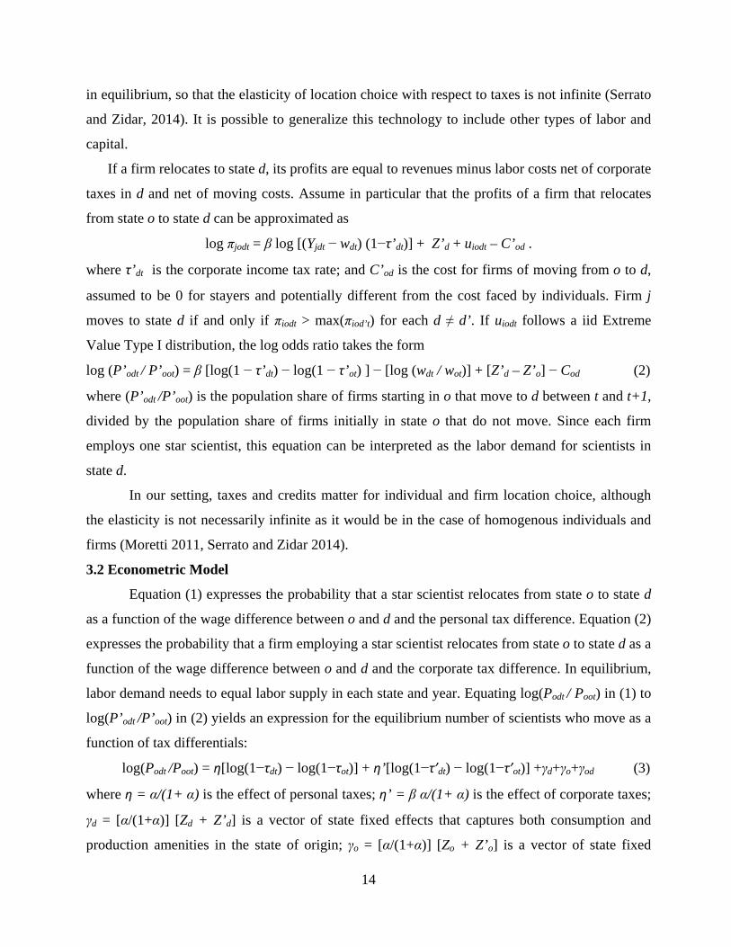
in equilibrium, so that the elasticity of location choice with respect to taxes is not infinite (Serrato
and Zidar, 2014). It is possible to generalize this technology to include other types of labor and
capital.
If a firm relocates to state d, its profits are equal to revenues minus labor costs net of corporate
taxes in d and net of moving costs. Assume in particular that the profits of a firm that relocates
from state o to state d can be approximated as
log πjodt = β log [(Yjdt − wdt) (1−τ’dt)] + Z’d + uiodt – C’od .
where τ’dt is the corporate income tax rate; and C’od is the cost for firms of moving from o to d,
assumed to be 0 for stayers and potentially different from the cost faced by individuals. Firm j
moves to state d if and only if πiodt > max(πiod’t) for each d ≠ d’. If uiodt follows a iid Extreme
Value Type I distribution, the log odds ratio takes the form
log (P’odt / P’oot) = β [log(1 − τ’dt) − log(1 − τ’ot) ] − [log (wdt / wot)] + [Z’d – Z’o] − Cod (2)
where (P’odt /P’oot) is the population share of firms starting in o that move to d between t and t+1,
divided by the population share of firms initially in state o that do not move. Since each firm
employs one star scientist, this equation can be interpreted as the labor demand for scientists in
state d.
In our setting, taxes and credits matter for individual and firm location choice, although
the elasticity is not necessarily infinite as it would be in the case of homogenous individuals and
firms (Moretti 2011, Serrato and Zidar 2014).
3.2 Econometric Model
Equation (1) expresses the probability that a star scientist relocates from state o to state d
as a function of the wage difference between o and d and the personal tax difference. Equation (2)
expresses the probability that a firm employing a star scientist relocates from state o to state d as a
function of the wage difference between o and d and the corporate tax difference. In equilibrium,
labor demand needs to equal labor supply in each state and year. Equating log(Podt / Poot) in (1) to
log(P’odt /P’oot) in (2) yields an expression for the equilibrium number of scientists who move as a
function of tax differentials:
log(Podt /Poot) = η[log(1−τdt) − log(1−τot)] + η’[log(1−τ’dt) − log(1−τ’ot)] +γd+γo+γod (3)
where η = α/(1+ α) is the effect of personal taxes; η’ = β α/(1+ α) is the effect of corporate taxes;
γd = [α/(1+α)] [Zd + Z’d] is a vector of state fixed effects that captures both consumption and
production amenities in the state of origin; γo = [α/(1+α)] [Zo + Z’o] is a vector of state fixed

15
effects that captures both consumption and production amenities in the state of destination; and
γod = −(Cod + C’od) is a vector of state-pair fixed effects that captures the cost of moving for
individuals and firms for each state pair.
Equation (3) represents our baseline econometric specification, although in some models,
we include additional controls. (To control for time-varying regional shocks, we augment
equation (3) by including region-pair*year effects. To control for time-varying state specific
shocks, in some models we augment it by including state-of-origin*year effects or state-of-
destination*year effects.)
In interpreting our estimates of the parameters η and η’, three important points need to be
considered. First, the parameters η and η’ are the reduced form effect of taxes on employment. As
such, their magnitude depends on labor demand and supply elasticities, which in turn are a
function of β and α. Changes in personal income taxes shift the supply of scientists to a specific
state and therefore involve a movement along the labor demand curve. The ultimate impact on the
equilibrium number of scientists depends on the slope of labor demand curve. If labor demand is
highly elastic, the change in scientists will be large. If demand is inelastic, the change in number
of scientist will be small − not because taxes don’t matter, but because with fixed demand the
only effect of the policy change is higher wages.
Similarly, changes in business taxes affect the demand of scientists in a given state and
therefore involve a movement along the supply curve. The ultimate impact on the equilibrium
number of scientists depends on the slope of labor supply curve. For a given shift in demand, the
change in number of scientists will be larger the more elastic is labor supply. Empirically, we
expect labor demand faced by a state to be elastic in the long run. Since in the long run firms can
locate in many states, local labor demand is likely to be significantly more elastic than labor
demand at the national level.
Although our estimates of η and η’ are reduced form estimates, they are the parameters of
interest for policy makers interested in quantifying employment losses that higher taxes might
cause.
A second point to consider is that our empirical models capture the long run effect of taxes.
The long run effects are likely to be larger than the immediate effect, because it takes time for
people and firms to move. In addition, some of the tax changes are temporary. Permanent tax
changes are likely to have stronger effects than temporary changes. Moreover, our models

16
measure not only the direct effect of taxes, but also any indirect effect operating through
agglomeration economies, if they exist. For example, consider the case where a tax cut results in
an increases in the number of biotech scientists in a state; and such exogenous increases makes
that state endogenously more attractive to other biotech scientists. Our estimates will reflect both
the direct (exogenous) effect and the indirect (endogenous) agglomeration effect.
A third point to keep in mind in interpreting our estimates is that variation in taxes may be
associated with variation in public services and local public goods. Our estimates need to be
interpreted as measuring the effect of taxes on scientist mobility after allowing for endogenous
changes in the supply of public services. If higher taxes mean better public services, our estimates
are a lower bound of the effect of taxes holding constant the amount of public services. Consider
for example the case where a state raise taxes in order to improve schools, parks and safety. If
scientists and their families value these services, the disincentive effect of higher taxes will be in
part off set by the improved amenities. In the extreme case where the value of the new public
services is equal to the tax increase, the disincentive effect disappears.
In general, however, the cost of taxation to high income taxpayers is unlikely to be identical to
the benefits of public services enjoyed by high income individuals. First, a significant part of state
taxation is progressive and redistributive in nature. High income individuals tend to pay higher
tax rates and receive less redistribution than low income individuals. Second, it is realistic to
assume that high income individuals are likely to consume less public services than low income
individuals. For example, high income individuals are more likely to send their children to private
schools than low income individuals. Finally, due to deadweight loss of taxation, and overall
inefficiency of the public sector, the disincentive effect will still exist, but it will be lower than the
pure monetary value of the tax increase.
Throughout the paper, our standard errors are robust and allow for two-way clustering by
origin*year and destination*year. This is necessary because in our data each origin and each
destination state appear 50 times in each year and states do not impose different tax rates on in-
migrants from different states. In addition, we present estimates that allow for serial correlation
over time, as emphasized by Bertrand, Duflo and Mullainathan (2004) and Kezdi (2004). We deal
with this possibility by clustering by origin-destination pair – thus allowing for unrestricted serial
correlation for each pair. Alternatively, in some models we allow for unrestricted serial
correlation by two-way clustering by origin and destination state.

17
With estimates of the parameters η and η’, it is straightforward to calculate the average
elasticity of the probability of moving with respect to the net-of-tax rate. For example, for
personal taxes the elasticity is
(4)
where P is the weighted average of over all (d,o,t) observations, weighting each combination
by the number of individuals in that observation cell. In our sample, P = 0.06, so the elasticities
will be very close to η. The revenue maximizing tax rate is the inverse of the elasticity.
4 Identification and Threats to Validity
Taxes are set by state legislatures, certainly not in random ways. The key concern is that there
are omitted determinants of scientist migration decisions that may be correlated with changes in
personal or corporate taxes. Our models control for permanent heterogeneity in migratory flows,
not just at the state level, but at the state pair level. In other words, we account not only for the
fact that in our sample period some states tend to lose scientists and other states tend to gain
scientists, but also for the typical migratory flow between every pair of states during our period.
For example, if star scientists tend to move to California from mid-western states because they
value local amenities like weather or because California has historically important clusters of
innovation-driven industries (e.g., Silicon Valley), state pair effects will account for these factors,
to the extent that they are permanent.
Of course, there may be omitted determinants of changes in migratory flows that are
correlated with changes in taxes. Consider the business cycle, for example, which in many states
is an important determinant of changes in taxes. If states tend to increase personal income taxes
during recessions, and scientists tend to leave the state during recessions, then our estimates
overestimate the true effect of taxes because they attribute to taxes some of the effect of
recessions. 10 On the other hand, if states are reluctant to impose higher taxes during recessions,
when local employers are struggling, then we underestimate the effect of taxes.
The possibility of unobserved labor demand shocks driven by local business cycle is probably
not a major issue because the overwhelming majority of star scientists work in the traded sector.
Shocks to the demand of star scientists are likely to reflect shocks that are national or global in
scope, and unlikely to reflect state specific shocks. For example, Google is based in California, 10 Diamond (2014) for example argues that local governments are more likely to extract rents during good times.
18
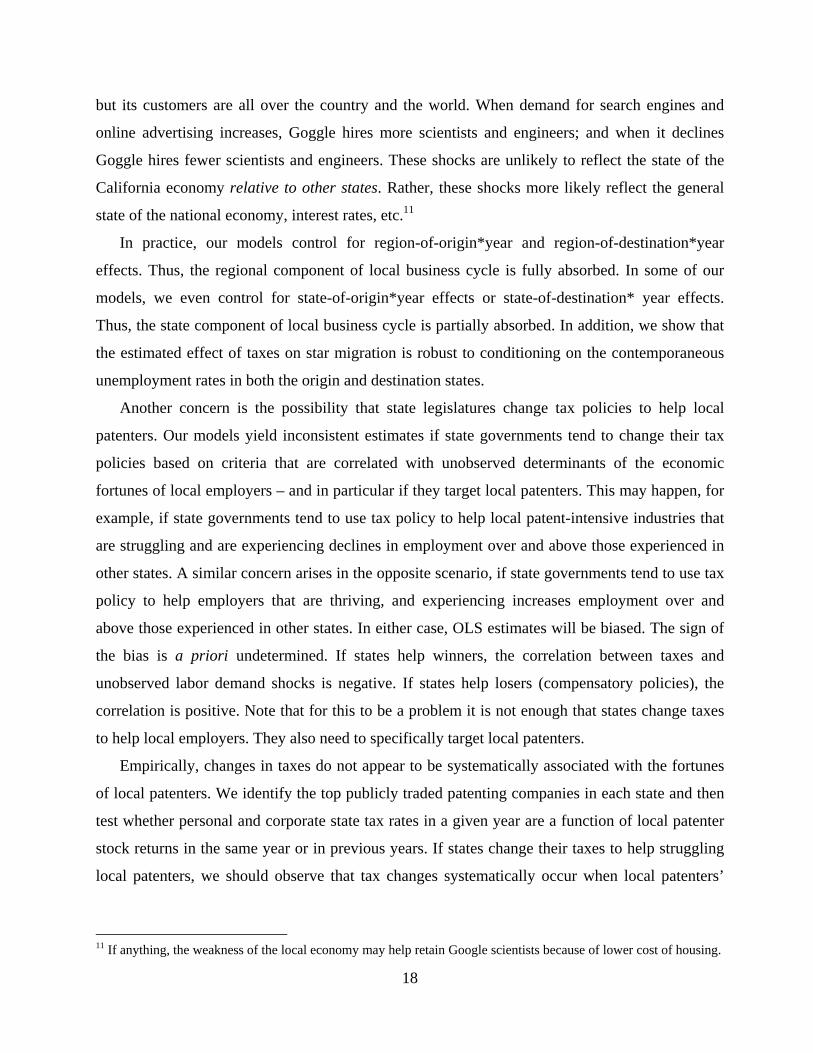
but its customers are all over the country and the world. When demand for search engines and
online advertising increases, Goggle hires more scientists and engineers; and when it declines
Goggle hires fewer scientists and engineers. These shocks are unlikely to reflect the state of the
California economy relative to other states. Rather, these shocks more likely reflect the general
state of the national economy, interest rates, etc.11
In practice, our models control for region-of-origin*year and region-of-destination*year
effects. Thus, the regional component of local business cycle is fully absorbed. In some of our
models, we even control for state-of-origin*year effects or state-of-destination* year effects.
Thus, the state component of local business cycle is partially absorbed. In addition, we show that
the estimated effect of taxes on star migration is robust to conditioning on the contemporaneous
unemployment rates in both the origin and destination states.
Another concern is the possibility that state legislatures change tax policies to help local
patenters. Our models yield inconsistent estimates if state governments tend to change their tax
policies based on criteria that are correlated with unobserved determinants of the economic
fortunes of local employers – and in particular if they target local patenters. This may happen, for
example, if state governments tend to use tax policy to help local patent-intensive industries that
are struggling and are experiencing declines in employment over and above those experienced in
other states. A similar concern arises in the opposite scenario, if state governments tend to use tax
policy to help employers that are thriving, and experiencing increases employment over and
above those experienced in other states. In either case, OLS estimates will be biased. The sign of
the bias is a priori undetermined. If states help winners, the correlation between taxes and
unobserved labor demand shocks is negative. If states help losers (compensatory policies), the
correlation is positive. Note that for this to be a problem it is not enough that states change taxes
to help local employers. They also need to specifically target local patenters.
Empirically, changes in taxes do not appear to be systematically associated with the fortunes
of local patenters. We identify the top publicly traded patenting companies in each state and then
test whether personal and corporate state tax rates in a given year are a function of local patenter
stock returns in the same year or in previous years. If states change their taxes to help struggling
local patenters, we should observe that tax changes systematically occur when local patenters’
11 If anything, the weakness of the local economy may help retain Google scientists because of lower cost of housing.

19
stock are under-performing. If states change their taxes to help thriving local patenters, we should
observe that tax change systematically occur when local patenters’ stock are under-performing.
We first identify the top five patent assignees (in terms of patent counts over the full 1977-
2010 sample) in each state. The majority of these assignees are publicly traded companies; for
those, we match by company name to the Compustat financial database. We then calculate the
sum of market capitalization over these top patenting companies, by state and by year. Finally, in
a state-by-year panel, we regress state tax rates (for each of our four tax variables) on
contemporaneous and lagged values of the percentage change in market capitalization of these
companies, along with state and year fixed effects.
The results are shown in Tables 2a to 2d. We find no evidence that any of these state tax
policies is systematically associated with the recent fortunes of local patenting companies.
Another potential concern is the possibility that changes in economic policies other than taxes
are correlated with taxes. For example, a pro-business state legislature could both cut taxes and
relax state level regulations on labor and the environment. In this case, our models would likely
overestimate the true effect of taxes. In this respect, models that control for state of origin*year
effects or state of destination* year effects are informative of the amount of bias. For example, if
an origin state both cut taxes and regulations, a model that includes origin*year effects will
account for it.
Of course, we can’t rule out with certainty that there are other omitted determinants of
changes in migratory flows that are correlated with changes in taxes. We provide indirect
evidence on the validity of our estimates with four specification tests.
First, we provide a specification test based on differences in the degree of tax
progressivity across states. In particular, we estimate models that include both changes in the
MTR for the top 99% of income and changes in the MTR for median income. Star scientists have
high income and should be significantly more sensitive to the MTR 99%. By contrast, if taxes did
not matter, and our estimates are entirely driven by omitted changes in other state policies, we
might find a significant effect of MTR 50%.
Second, we provide a specification test based on the fact that corporate taxes should affect
some scientists but not others.

20
(i) On the most obvious level, changes in corporate taxes, ITC and R&D credits should affect
scientists in the private sector but scientists employed by universities and government agencies,
which are mostly non-profit and therefore unaffected by corporate income taxes.
(ii) Individual inventors provide an even sharper test: they should not be sensitive to corporate
taxes and ITC but they should be sensitive to R&D tax credits.
(iii) Moreover, we exploit variation in the apportionment formula. A testable hypothesis is
that corporations’ demand for labor, including star scientists, should be sensitive to corporate tax
rates in states where payroll is one of the apportionment factors and should be less sensitive in
other states.
Third, we exploit close elections. In particular, we isolate only the variation in tax changes that
stems from a change in the party of the governor or the majority of the state legislature resulting
from a close election. The idea is that small variation in vote share can generate large changes in
policy when the governor’s or majority’s party change.
Finally, we exploit the timing of tax changes and we test for pre-trends.
5. Main Empirical Results
5.1 Graphical Evidence
Cross-sectional analysis reveals little relationship between tax levels and number of scientists.
Compare Figures 1 and 2 – which display map of personal and corporate taxes by state in 2006 –
with Figure 5 – which displays where top scientists were located in the same year. A cross-
sectional analysis, however, can be misleading because it fails to account for other important
differences across states, such as in amenities, agglomeration economies, industry composition,
market size, the presence of top research institutions, etc.
The variation that we use in the data is based on changes over time in taxes. In Figure 7 we
show a series of bin-scatterplots of the log odds-ratio against the log net-of-tax rate after
conditioning on state-pair and year fixed effects. In other words, we demean the log odds-ratio
and the log net-of-tax rate by their within-pair and within-year sample means. The two panels on
the far left show outmigration between a given origin-destination pair versus the indicated net-of-
tax rate in the origin state. The two panels in the center use the destination state’s tax rate on the
x-axis. If taxes affect the migration decisions of scientists, one would expect the relationship
between origin net-of-tax rates and outmigration to be negative, as higher net-of-tax rates in the
origin state (i.e. lower taxes in origin state) result in less outmigration. Similarly, one would

21
expect the effect of destination net-of-tax rates to be positive, as higher net-of-tax rates in the
destination state (i.e. lower taxes in destination state) result in more migration to that state.
Empirically, this is what we observe.
The two panels on the far right of the figure show the same type of bin-scatterplots except that
the measure on the x-axis is now the difference between the destination state’s log net-of-tax rate
and the origin state’s log net-of-tax rate. This specification is equivalent to those in the first four
panels, but it is more parsimonious in that it forces the effect of tax changes in the origin and
destination state to be the same but of opposite sign. The plots shows that higher destination-
origin net-of-tax rate (after-tax income) differentials are associated with higher origin-to-
destination migration.
5.2 Baseline Regressions
The baseline regression results are shown in Table 3. Each cell – consisting of a coefficient
and standard error – represents a single regression of the log odds ratio on the pairwise
differential between the log of the net-of-tax rates in the destination and origin states for a given
tax variable (indicated in the row heading). In other words, we estimate variants of equation (3) in
Section 3. All regressions contain year fixed effects.
The regressions underlying column (1) do not condition on state or state-pair fixed effects and
therefore are based on cross-sectional variation. In this case, the estimated coefficient on the net-
of-tax rate for personal and corporate taxes is negative and significant – contrary to expectations
of a positive effect from after-tax income.
Column (2) adds state of origin and destination fixed effects, while column 3 adds state-pair
fixed effects. Now the coefficients on all net-of-tax rate variables becomes positive and
statistically different from zero at conventional levels. Column (3) is equivalent to the fit lines
shown in the two far-right panels of Figure 7. Columns (4) to (6) show estimates conditional on a
year-specific fixed effect for the region of the origin state (using Census Bureau’s nine-region
categorization)(column 4), a year-specific fixed effect for the region of the destination state
(column 5), a year-specific fixed effect for the pair defined by the origin region and destination
region (column 6).
Our preferred specification is that of column (6), which absorbs both state-pair permanent
characteristics as well as time-varying year-specific shocks that are specific to each region-pair.
The coefficient on the 99th MTR net-of-tax rate is 1.78 and is significant at the 1% level. Given
22
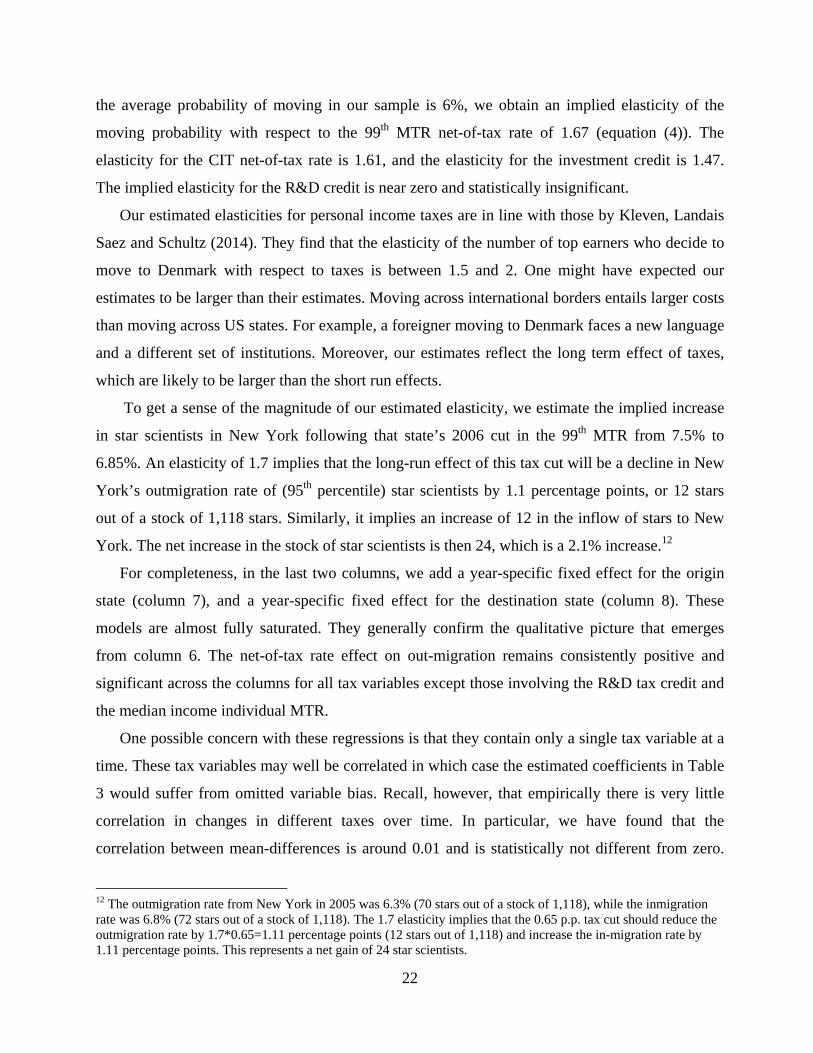
the average probability of moving in our sample is 6%, we obtain an implied elasticity of the
moving probability with respect to the 99th MTR net-of-tax rate of 1.67 (equation (4)). The
elasticity for the CIT net-of-tax rate is 1.61, and the elasticity for the investment credit is 1.47.
The implied elasticity for the R&D credit is near zero and statistically insignificant.
Our estimated elasticities for personal income taxes are in line with those by Kleven, Landais
Saez and Schultz (2014). They find that the elasticity of the number of top earners who decide to
move to Denmark with respect to taxes is between 1.5 and 2. One might have expected our
estimates to be larger than their estimates. Moving across international borders entails larger costs
than moving across US states. For example, a foreigner moving to Denmark faces a new language
and a different set of institutions. Moreover, our estimates reflect the long term effect of taxes,
which are likely to be larger than the short run effects.
To get a sense of the magnitude of our estimated elasticity, we estimate the implied increase
in star scientists in New York following that state’s 2006 cut in the 99th MTR from 7.5% to
6.85%. An elasticity of 1.7 implies that the long-run effect of this tax cut will be a decline in New
York’s outmigration rate of (95th percentile) star scientists by 1.1 percentage points, or 12 stars
out of a stock of 1,118 stars. Similarly, it implies an increase of 12 in the inflow of stars to New
York. The net increase in the stock of star scientists is then 24, which is a 2.1% increase.12
For completeness, in the last two columns, we add a year-specific fixed effect for the origin
state (column 7), and a year-specific fixed effect for the destination state (column 8). These
models are almost fully saturated. They generally confirm the qualitative picture that emerges
from column 6. The net-of-tax rate effect on out-migration remains consistently positive and
significant across the columns for all tax variables except those involving the R&D tax credit and
the median income individual MTR.
One possible concern with these regressions is that they contain only a single tax variable at a
time. These tax variables may well be correlated in which case the estimated coefficients in Table
3 would suffer from omitted variable bias. Recall, however, that empirically there is very little
correlation in changes in different taxes over time. In particular, we have found that the
correlation between mean-differences is around 0.01 and is statistically not different from zero.
12 The outmigration rate from New York in 2005 was 6.3% (70 stars out of a stock of 1,118), while the inmigration rate was 6.8% (72 stars out of a stock of 1,118). The 1.7 elasticity implies that the 0.65 p.p. tax cut should reduce the outmigration rate by 1.7*0.65=1.11 percentage points (12 stars out of 1,118) and increase the in-migration rate by 1.11 percentage points. This represents a net gain of 24 star scientists.

23
Nonetheless, in Table 4, we include personal income tax variable along with the three business
tax variables jointly in the same regression. As before, we find strong and robust evidence of a
positive and significant effect of the net-of-tax rate on out-migration for the top-income individual
MTR, the corporate tax, and the investment tax credit. The estimated effect of the R&D tax credit
is less robust. For all of the tax variables, the point estimates and implied elasticities are similar to
those found in Table 3.
Next, we relax the assumption that destination and origin taxes have symmetric effects on
pairwise migration. We repeat the regressions underlying Table 3 but relax the restriction that the
log net-of-tax rate in the destination state has an equal but of opposite sign effect as that in the
origin state. The results are shown in Table 5.13 Column (1) shows the results of a specification
including state-pair fixed effects while column (2) adds region-pair*year fixed effects. For both
the individual and corporate net-of-tax rates, we find evidence of a negative and significant effect
from the origin state tax. That is, out-migration tends to fall as net-of-tax rates, and hence after-
tax incomes, rise in the origin state. Out-migration tends to rise as net-of-tax rates rise in potential
destination states, though the magnitude of this effect is smaller. It is statistically insignificant for
the CIT when region-pair*year fixed effects are included. The finding that the effect of tax change
in the origin state is larger than the effect in the destination state might indicate that individuals
have more information on taxes in their state of residence – after all, there are 49 potential
destination states, and they frequently change their rates.
The two tax credit variables, the relative importance of destination and origin state taxes is
reversed, with the origin state effect smaller and often insignificant. The fact that tax incentives
have a stronger “pull” effect is probably not too surprising: tax credits are designed to attract and
targeted to out-of-state businesses doing site selection searches, and often advertised to specific
industries.
5.3 Specifications Tests
Top-Income MTR vs Median-Income MTR. In Table 6, we report the results from regressions
containing both the top-income MTR and the median-income MTR simultaneously. We test
whether star scientists’ locational choices are more sensitive to top-income tax rates than to
middle-income tax rates. Although we don’t have direct information on star scientists’ actual
13 For these specifications we cannot include either origin-state*year fixed effects or destination-state*year fixed effects as that would leave no variation with which to identify the coefficients of interest.

24
income, we expect them to be at the very high end of the income distribution. Thus, we expect
that changes in the 99th MTR should matter more than changes in the 50th percentile MTR.
Finding that changes in the 50th percentile MTR matter more would cast doubt on the validity of
our estimates.
Each column in Table 6 shows the results from three different regressions: 99.9th percentile
MTR vs. 50th percentile MTR (top panel), 99th percentile MTR vs. 50th percentile MTR (middle
panel), and 95th percentile MTR vs. 50th percentile MTR (bottom panel). The regressions
underlying column (1) include state-pair and year fixed effects (as in column 3 of Tables 3-4)
while those underlying column (2) add region-pair*year fixed effects (as in column 6 of Tables 3-
4). In all cases, we find the top-income MTR differential to have a positive and significant effect
on out-migration. The median-income MTR, on the other hand, is generally small and statistically
insignificant.
Specification Tests on Business Taxes. Next we consider several specifications tests based on
business taxes. The results in Tables 3 and 4 indicate a strong effect from the corporate income
tax rate and the investment tax credit rate and a more modest effect from the R&D tax credit. To
mitigate concerns that these results reflect some spurious correlation, we perform several
additional hypotheses tests.
First, we exploit the fact that states vary in whether, and how much, employment location
matters for corporate taxation of companies generating income in more than one state. As we
described in the previous section, a corporation in a given state must determine what share of its
national taxable income to apportion to that state based on the state’s apportionment formula,
which is a weighted average of the state’s shares of the company’s national payroll, property, and
sales. The weight on employment (payroll) varies across states and over time, and ranges from
zero to one-third. With a zero weight, a corporation’s tax liablity in a given state is independent of
its level of employment in that state (conditional on having a tax liability in that state at all).
Therefore, a testable hypothesis is that corporations’ demand for labor, including star scientists,
should be more sensitive to corporate tax rates in states with larger apportionment weights on
payroll.
To test this hypothesis, we construct an indicator variable that equals one if the origin state, in
that year, has a payroll weight equal to the traditional formula’s one-third weight and that equals
zero otherwise. (About half of our sample have a one-third payroll weight; the other half generally

25
have either zero or 0.1.) We construct an analogous variable for destination states. We then
estimate the pair fixed effects model as in the CIT rows of Table 3, Column (2) but adding these
two indicator variables as well as their interactions with the origin and destination CIT net-of-tax
rates. The results are shown in Table 7. The only difference between the two columns is whether
non-CIT tax rates are included. We find that the origin state’s net-of-tax corporate rate reduces
outmigration significantly more in origin states with a relatively high apportionment weight on
payroll. Similarly, the destination state’s net-of-tax corporate rate increases migration to that state
significantly more when the destination state has a high payroll weight. The results are robust to
conditioning on non-CIT rates (see column 2).
Next, we investigate whether migration of star scientists who (initially) work in the private
sector are more sensitive to business taxes than are scientists who work for not-for-profit
organizations, like academia and government. The COMETS patent database classifies the
organization type of the patent owner into the following categories: firm, research institution,
government, or other. Furthermore, it identifies the actual name of the organization. This allows
us to additionally screen out firms that appear to be pass-through entities (such as S corporations)
and not standard C corporations, and therefore are not subject to the corporate income tax.
Specifically, we screen out organizations (patent assignees) whose name in the patent record
contains “limited liability corporation,” “limited liability partnership”, and related abbreviations.
The results are shown in Table 8. We find that all three business tax policies – the corporate
income tax, the investment tax credit, and the R&D tax credit – significantly affect migration for
star scientists working for corporations but have no significant effect on migration of stars
working for academic or governmental institutions.
In Column (4), we look at migration of individual inventors – that is, patenters who own their
own patent rather than assigning it to some organization. Consistent with our prior that these
inventors would not be subject to the corporate income tax rate, their migration appears to be
insensitive to the corporate income tax rate.14 In most states, both individual and corporate
income taxpayers can claim R&D tax credits for qualified expenditures. Many individual
inventors may have non-trivial R&D expenditures (especially given that R&D includes their own
labor expenses) and hence could be sensitive to the R&D tax credit. The results in column (4)
14 The only case in which CIT would matter for an individual inventor is the case where the inventor plans to create a firm in the future and is forward looking enough to take future CIT into consideration.

26
suggest this is the case: the coefficient on the investment net-of-tax credit rate is insignificant
while the coefficient on the R&D net-of-tax credit rate is relatively small but statistically
significant.15
We attempted to identify pass-through entities based on the name of the firm reported on the
patent application. Unfortunately, the pass-through sample is too small to allow meaningful
estimates. The small sample size reflects the fact that we are only able to identify pass-throughs if
they have an obvious identifier like “Limited Liability,” “LLP”, or “LLC” in their organization
name listed on the patent (under patent assignee). Moreover, pass-through entities, while common
for professional services (doctor, lawyers, etc.), are not very common in high tech fields. We also
miss all pass-through subsidiaries of large firms, if patents are filed under the parent firm.
5.4 Isolating Variation in Taxes that Comes from Close Elections
We turn to a regression discontinuity design based on the idea that (1) state governments
controlled by the Republican (Democratic) party are more likely to enact tax cuts (increases) and
(2) political party control is determined by sharp cut-offs. The party in control of the governor’s
office is determined by the vote share in the most recent election, while the party in control of
each legislative chamber is determined by the share of seats in the chamber controlled by the
majority party. In each case, party control switches discontinuously at 50%.
We use an instrumental variable setting where identifiers for Republican control of the
governor office, the state House, and the state Senate are the excluded instruments, and we
condition on the margin of victory in most recent gubernatorial election and the percentages of
seats held by the majority party in the state House and Senate. These models isolate the variation
in tax changes that stems only from a change in the party of the governor or the majority of the
state legislature resulting from a close election or shift in legislative seats close to 50%.
The results are provided in Table 9. To economize on space, the table does not show the full
first-stage results; we suffice to report here that the coefficients on the Republican dummies are
consistent with the prior that tax decreases are more likely under Republican governments. We
also find that the party of the governor and the state house tend to be more important than the
party of the state senate. The first-stage F statistics are well above standard critical values for
15 While not shown in these tables, we also estimated the effect of the individual income net-of-tax rate, for the 99th percentile, on migration of individual inventors. This net-of-tax rate has a coefficient of 2.08 (with a standard error of 0.67), roughly similar to the coefficients on the individual MTR from the full sample.

27
weak-instrument bias except in the case of the CIT, for which the F statistic is below standard
critical values.
The IV results are qualitatively similar, though larger and much less precise, than the
corresponding OLS results, with the exception of the R&D tax credit which has an unexpected
negative sign. The coefficients are statistically significant for the MTR (and R&D credit). The
coefficient on the CIT net-of-tax differential is economically large but not statistically significant,
which is not surprising given the low first-stage fit for the CIT. We take away from these results
that, at least for the MTR and CIT, IV estimates are qualitative consistent with our baseline
estimates, but not precise enough to draw definitive conclusions.
5.5 Robustness
In this section, we assess whether our findings are robust to a number of alternative
specifications and alternative samples.
First, we consider whether our baseline results are sensitive to the precise definition of “stars.”
So far, we have defined stars as scientists in the top 5% of patent counts over the prior ten years.
Appendix Tables A2 and A3 repeat the same set of regressions as in Table 3 but using a sample
where stars are defined as those in the top 1% or 10% of the distribution. The results are generally
similar to the baseline results. The effects are somewhat larger for the top 1% stars, probably
because they are likely to have higher incomes. We can also define stars based on citation counts
instead of patent counts in order to include scientists that produce fewer but higher quality patents
and exclude scientists that produce many but less influential patents. Appendix Table A4 shows
that the estimated effects are similar but slightly larger than the baseline results, possibly because
these stars have higher average incomes than the baseline set of stars.
In Columns (2) and (3) of Table 10 we probe the robustness of our baseline standard errors to
alternative assumptions about potential correlation of the residuals. For ease of comparison, we
redisplay the baseline results in Column (1). Recall that in our baseline results allow for residuals
to be clustered, within year, by origin-state and by destination-state. This accounts for the fact
that the origin tax used in the net-of-tax differential regressor is the same, within a year, across all
pairs involving that origin state, and similarly for the destination tax. In Column (2), we allow this
two-way clustering by origin and by destination not just within a year but over the full sample.
This is an extremely broad level of clustering as it allows for any type of serial correlation of
errors across time in addition to the cross-sectional dependence across pairs. This results in about

28
a tripling of the standard errors. The effects for the individual top MTR remain statistically
significant but at the 10% level. The effects for the three business tax variables lose their
statistical significance. In Column (3), we cluster by state-pair. This allows for any type of serial
correlation of errors but rules out cross-sectional dependence. We obtain standard errors very
similar to the baseline case. We infer from this that the statistical significance of our estimated
migration effects is robust to either cross-sectional dependence or serial correlation, but it is less
robust to allowing for both simultaneously.
In Column (4), we assess how the baseline results change if one gives more weight to
observations from state-pairs with larger bilateral migration flows. Specifically, we weight each
pair of states based on the average outflow of stars over the full sample. This weighting leads to
somewhat larger estimated effects.
In column (5), we condition on current origin and destination state economic conditions via
the unemployment rate and the population in each state. We opt not to include these variables in
our baseline regressions because they may well reflect endogenous responses of the state
economy to changes in state taxes.
Column (6) shows that results do not change when we drop post-2006 observations from
the sample, indicating that our estimates are not driven by the Great Recession.16
In column (7), we use an alternative patent database, constructed by Li, et al. (2014), that
applies a disambiguation algorithm to the reported scientist (patent inventor) names to attempt to
(1) separately identify multiple assignees who share a common name (e.g., John Smith) and (2)
identify unique assignees who report their name slightly differently on different patents (e.g.,
Alex Bell, Alexander Bell, Alexander G. Bell, Alexander Graham Bell, etc.). Using this
alternative database, we find somewhat larger tax effects for the personal tax rates and somewhat
smaller tax effects for the CIT and the tax credits.
Finally, Appendix Table A5 shows estimates based on average tax rates, instead of
marginal tax rates.
6 Timing of the Effects
16 Some eventually-granted patents are missing in the COMETS patent database because at the time of its construction many patents applied for in 2007 – 2010 (and likely a small number from even earlier years) had not yet been granted and hence are not included in this database. This affects both the numerator and the denominator of the odds ratio that we use as our dependent variable, so it is expected to represent classical measurement error.

29
We now explore the timing of the migration responses to tax changes. We start by
investigating how the contemporaneous effect of tax changes on migration depends on the length
of the time interval considered. We then trace the impulse response of scientist migration to tax
changes. This allows us to determine exactly how long it takes for a tax change to affect mobility
as well as test for pre-trends. In this section, we shift from the mean-difference model considered
in the previous section to a time-difference (e.g., first-difference) model. Both are standard
empirical models for eliminating fixed effects and are asymptotically equivalent, but the time-
difference estimator avoids the well-known finite sample bias associated with estimating dynamic
panel models via mean-differencing (Nickell 1981).
Appendix Figures 1 and 2 show how the estimated tax effects differ as one varies the length of
the time-differencing (i.e., short-differences versus long-differences). Each data point in the graph
is from a separate regression based on difference length of differencing. For example, the estimate
for length of differencing = 5 is from a regression of 5-year changes in mobility on 5-year
changes in the relevant tax variable. For the individual MTR, the ITC, and the R&D credit, first-
differencing yields near-zero and statistically insignificant tax effects, while longer differencing,
especially time differences above 5 years, yields net-of-tax rate elasticities similar to our baseline
mean-differencing results. This is to be expected, as our baseline estimates in levels are to be
interpreted as long run estimates.
The larger effects uncovered by long difference models reflect the fact that migration
responses to tax shocks are likely to be gradual, as it takes time for scientists and firms to
relocate. They also reflect the fact that short-differences, such as a one-year first-difference, are
more likely to reflect temporary tax changes or increments of a multi-year phased-in tax change,
while long-differences are more likely to reflect permanent, or at least persistent, tax changes. We
expect mobility to be more sensitive to permanent tax changes.
We conclude that first-differences are too high frequency to adequately capture the full effect
of tax changes on outmigration. By contrast, long-differencing, especially using differences in the
neighborhood of five years, yields results similar to mean-differencing and arguably is better
suited for exploring the full dynamic responses to net-of-tax rate shocks.
We now turn to exact timing of the migration response. We use the direct projections
estimator (Jorda 2005) to estimate the impulse response function of outmigration with respect to
tax change treatments. Specifically, we estimate the model:

30
(4)
where the dependent variable is the change in outmigration (log odds-ratio) from before the
treatment, , to periods after the treatment. represents a year-specific fixed effect
for each pair of regions defined by the origin state’s region and the destination state’s region. We
estimate the regression separately for each horizon from 0 to 10. k is the duration of the
treatment period. In typical event studies, is assumed to equal one but we also consider
durations of 3 years and 5 years. To be consistent with the our previous estimates, we condition
on region-pair*year effects. To test for pre-trends, we extend this estimator by looking at the
association between the treatment (occurring from to ) and changes in outmigration over
intervals prior to when the treatment began (i.e., prior to ).
Results for the top individual MTR and the CIT are in Figures 8 and 9. Results for the R&D
and investment credits are in Figures 10 and 11. There are three panels in each figure, one where
treatment duration is assumed to be 1 year, one where it is assumed to be 3 years, and one where
it is assumed to be 5 years. As we have seen, one year tax changes are likely too noisy to be
informative. Given the results above, our preferred specifications are the one for 3 or 5 years.
Note that in these models, the years before treatment are the ones prior to t-3 and t-5, respectively.
When tax changes are measured by either three- or five-year changes, clear dynamic patterns
emerge. First, for all four tax variables star outmigration shows no pre-trends. Second, star
migration rises after the change and keeps growing over time. This likely reflects the fact that it
takes time for people and firms to relocate in response to a tax change.
For the individual MTR, the CIT, and the R&D credit, outmigration begins to rise shortly
after the treatment period and continues to grow for at least 10 years. For investment credits,
outmigration’s response begins almost immediately upon the start of a tax change, grows up to
about five years after the end of the tax change, and then gradually declines through the end of the
ten-year horizon. The more immediate response to investment credits could reflect the fact that
changes in (typically enactments of) these credits, in contrast to changes in individual and
corporate income tax rates, are nearly always permanent and are fully phased-in the first year.
In models where the treatments are defined by one-year changes, the estimated impulse
response is generally positive, as expected, but imprecisely estimated and showing no clear
dynamic pattern.

31
7. Conclusions
Using data on the universe of U.S. patents filed between 1976 and 2010, we quantify how
sensitive is internal migration by star scientist to changes in personal and business tax
differentials across states. We uncover large, stable, and precisely estimated effects of personal
and corporate taxes on star scientists’ migration patterns. The long run elasticity of mobility
relative to taxes is 1.6 for personal income taxes, 2.3 for state corporate income tax and 2.6 for the
investment tax credit. These elasticities are economically large and significantly larger than the
conventional labor supply elasticity. The effect on mobility is small in the short run, and tends to
grow over time.
While we can’t rule out that our estimates are biased by unobserved demand or supply shocks,
a number of additional pieces of evidence lend credibility to a causal interpretation of our
estimates. First, we find no evidence of pre-trends: Changes in mobility follow changes in taxes
and do not to precede them. Second, consistent with their high income, star scientists migratory
flows are sensitive to changes in the 99th percentile marginal tax rate, but are insensitive to
changes in taxes for the median income. Third, the effect of corporate income taxes is
concentrated among private sector inventors: no effect is found on academic and government
researchers. Fourth, corporate taxes only matter in states where the wage bill enters the state’s
formula for apportioning multi-state income. No effect is found in states that apportion income
based only on sales (in which case labor’s location has little or no effect on the tax bill). We also
find no evidence that changes in state taxes are correlated with changes in the fortunes of local
firms in the innovation sector in the years leading up to the tax change.
Overall, we conclude that state taxes have significant effect of the geographical location of
star scientists and possibly other highly skilled workers. While there are many other factors that
drive when innovative individual and innovative companies decide to locate, there are enough
firms and workers on the margin that relative taxes matter.

32
References
Alvaredo, F, A Atkinson, T Piketty, and E Saez (2013) “The Top 1 Percent in International and
Historical Perspective.” Journal of Economic Perspectives, AEA, 27(3), 3-20
Bakija, Jon, and Joel Slemrod (2004) “Do the Rich Flee from High State Taxes? Evidence from
Federal Estate Tax Returns.” NBER Working Papers 10645.
Bartik, Timothy J. (1991). “Who Benefits from State and Local Economic Development
Policies?” Kalamazoo: W.E. Upjohn Institute for Employment Research.
Bayer Pat and Robert McMillan (2012) “Tiebout Sorting and Neighborhood Stratification,”
Journal of Public Economics: 96: 1129-43
Chirinko, Robert, and Daniel J. Wilson. “State Investment Tax Incentives: A Zero‐Sum Game?”
Journal of Public Economics 92(12), Dec. 2008, pp. 2362‐2384.
Cohen, Roger, Andrew Lai, and Charles Steindel. 2011. “The Effects of Marginal Tax Rates on
Interstate Migration in the U.S.” Unpublished.
Cohen, Wes “Fifty Years of Empirical Studies of Innovative Activity and Performance,” in
Handbook of Economics of Innovation, Vol. 1, 2010, pp. 129-213.
Diamond, Rebecca “The Determinants and Welfare Implications of US Workers' Diverging
Location Choices by Skill: 1980-2000”, mimeo 2015.
Diamond, Rebecca “Housing Supply Elasticity and Rent Extraction by State Governments,” 2014.
Duranton, Gilles, Laurent Gobillon & Henry G. Overman, 2011. "Assessing the Effects of Local
Taxation using Microgeographic Data," Economic Journal, vol. 121(555), pages 1017-1046.
Duranton, Gilles, Overman, Henry G., 2005. Testing for localization using microgeographic data.
Review of Economic Studies 72 (4), 1079-1106.
Duranton Gilles. “California Dreamin': The feeble case for cluster policies” Review of Economic
Statistics, 2011, 3(1), 3-45.
Faulk, Dagney. “Do State Economic Development Incentives Create Jobs? An Analysis of State
Employment Tax Credits. National Tax Journal. 2002.
Gideon, Michael S. (2014). “Uncovering Heterogeneity in Income Tax Perceptions.” Unpublished
Manuscript, University of Michigan.
Griliches, Zvi “R&D and Productivity: The Econometric Evidence” University of Chicago Press
Volume, January 1998

33
Head, K., Ries, J., and Swenson, D., 1999. Attracting foreign manufacturing: investment
promotion and agglomeration. Regional Science and Urban Economics 29 (2), 197 – 218.
Helsley, Robert W. and William C. Strange, "Matching and Agglomeration Economics in a
System of Cities," Regional Science and Urban Economics, 20,1990, pp. 189-212.
Haughwout, Andrew, Robert Inman, Steven Craig, and Thomas Luce. 2004. “Local Revenue
Hills: Evidence from Four U.S. Cities.” Review of Economics and Statistics 86 (2): 570–85.
Kaplan, G and S Schulhofer-Wohl (2013) “The Age-Time-Cohort Problem and the Identification
of Structural Parameters in Life-Cycle Models.” WP 707, Fed. Res. Bank of Minneapolis
Kirchgassner, G and W W. Pommerehne (1996) “Tax Harmonization and Tax Competition in the
European Union: Lessons from Switzerland.” Journal of Public Economics, 60(3), 351-71
Kleven, Henrik Jacobsen, Camille Landais, and Emmanuel Saez “Taxation and International
Migration of Superstars: Evidence from the European Football Market” AER 103(5), 2013.
Kleven, H J, C Landais, E Saez, and E A Schultz (2014) “Migration and Wage Effects of Taxing
Top Earnings: Evidence from the Foreigners’ Tax Scheme in Denmark” QJE 129(1): 333-78
Liebig, T, P A. Puhani, and A Sousa-Poza (2007) “Taxation and Internal Migration- Evidence
from the Swiss Census using Variation in Income Tax Rates.” J. of Reg. Science
Li, Lai, D’Amour, Doolin, Sun, Torvik, Yu, and Fleming (2014) “Disambiguation and Co-
authorship Networks of the US Patent Inventor Database ” Research Policy 43, 941-955
Moretti, Enrico (2011). “Local labor Markets,” Handbook of Labor Economics.
Moretti, E, and D. Wilson (2014) "State Incentives for Innovation, Star Scientists and Jobs:
Evidence from Biotech", The Journal of Urban Economics, forthcoming
Nickell, (1981) “Biases in Dynamic Models with Fixed Effects.” Econometrica, 49, 1417-1426
Suárez Serrato, Juan Carlos, “Taxation, Entrepreneurship, and the Choice of Organizational
Form” (2014)
Suárez Serrato, Juan Carlos, Owen Zidar “State Corporate Taxes, Firm Mobility, and Innovation
Productivity: Evidence from US patent data” (2015)
Suárez Serrato, Juan Carlos, and Owen Zidar (2014), “Who Benefits from State Corporate Tax
Cuts? A Local Labor Market Approach with Heterogeneous Firms?”, mimeo, U of Chicago.
Varner, Charles, and Cristobal Young (2012) “Millionaire Migration in California: The Impact of
Top Tax Rates.” Working Paper. Stanford University Center on Poverty and Inequality.

34
Wilson, Daniel J. (2009). “Beggar Thy Neighbor? The In-State, Out-of-State, and Aggregate
Effects of R&D Tax Credits.” Review of Economics and Statistics 91(2), 431-436.
Young, Christobal, and Charles Varner (2011) “Millionaire Migration and State Taxation of Top
Incomes: Evidence from a Natural Experiment.” National Tax Journal, 64(2, part 1) p255-284
Zucker, Lynne G, Michael R. Darby, and Marilynn B. Brewer, 1998. "Intellectual Human Capital
and the Birth of U.S. Biotechnology Enterprises,"AER, vol. 88(1), pages 290-306.
Zucker, Lynne G, Michael R. Darby, “Movement of Star Scientists and Engineers and High Tech
Firm Entry”, NBER WP, 2006.
Zucker, Lynne G, Michael R. Darby, and Jason Fong, 2011. “Communitywide Database Designs
for Tracking Innovation Impact: COMETS, STARS and Nanobank.”NBER WP 17404.

Table 1: Average Annual Outflow of Star Scientists, 1997-2006
Destination StateOrigin State California Illinois Massachusetts Michigan Minnesota New Jersey New York Ohio Pennsylvania Texas
California 4767 13 24 10 9 17 21 8 12 25Illinois 14 649 4 2 2 2 4 2 2 5Massachusetts 25 3 873 2 3 4 5 2 4 4Michigan 12 2 3 654 2 2 3 2 2 4Minnesota 13 3 2 3 768 2 2 2 1 4New Jersey 23 2 7 2 1 879 8 2 6 4New York 25 3 6 4 3 10 1629 4 3 7Ohio 8 2 2 3 1 2 2 600 3 3Pennsylvania 13 2 4 1 1 5 4 3 679 3Texas 26 3 5 5 4 5 7 3 3 1166

Table 2a: CIT Regressed on Annual Stock Return of Top Patenters
No Lags No Lags 1-year Lag 1-year Lag 1-4 years Lag 1-4 years LagNo Fixed Effects Year, State FEs No Fixed Effects Year, State FEs No Fixed Effects Year, State FEs
Annual Stock Return Growth -0.0001 0.0002 -0.0001 0.0002 -0.0001 0.0001(0.0008) (0.0002) (0.0008) (0.0002) (0.0009) (0.0002)
Annual Stock Return Growth- 1 year lag -0.0001 0.0000 -0.0001 0.0000(0.0009) (0.0002) (0.0009) (0.0002)
Annual Stock Return Growth- 2 year lag -0.0002 0.0001(0.0009) (0.0002)
Annual Stock Return Growth- 3 year lag -0.0003 0.0000(0.0009) (0.0002)
Annual Stock Return Growth- 4 year lag -0.0003 0.0000(0.0009) (0.0002)
Joint Sig. p-value .8787 .9202 .9899 .9964∗ p < 0.10, ∗∗ p < 0.05, ∗∗∗ p < 0.01
Each column is a separate regression. Sample consists of 1527 observations over 50 states and 33 years
Table 2b: MTR (99th Percentile) Regressed on Annual Stock Return of Top Patenters
No Lags No Lags 1-year Lag 1-year Lag 1-4 years Lag 1-4 years LagNo Fixed Effects Year, State FEs No Fixed Effects Year, State FEs No Fixed Effects Year, State FEs
Annual Stock Return Growth 0.0010 0.0001 0.0011 0.0001 0.0008 -0.0000(0.0010) (0.0003) (0.0010) (0.0003) (0.0009) (0.0003)
Annual Stock Return Growth- 1 year lag 0.0010 0.0001 0.0009 -0.0000(0.0010) (0.0003) (0.0009) (0.0003)
Annual Stock Return Growth- 2 year lag 0.0010 0.0001(0.0009) (0.0003)
Annual Stock Return Growth- 3 year lag 0.0011 0.0002(0.0009) (0.0003)
Annual Stock Return Growth- 4 year lag 0.0009 0.0001(0.0009) (0.0003)
Joint Sig. p-value .3096 .7801 .4205 .9629∗ p < 0.10, ∗∗ p < 0.05, ∗∗∗ p < 0.01
Each column is a separate regression. Sample consists of 1527 observations over 50 states and 33 years

Table 2c: ITC Regressed on Annual Stock Return of Top Patenters
No Lags No Lags 1-year Lag 1-year Lag 1-4 years Lag 1-4 years LagNo Fixed Effects Year, State FEs No Fixed Effects Year, State FEs No Fixed Effects Year, State FEs
Annual Stock Return Growth 0.0002 0.0003 0.0002 0.0003 0.0002 0.0005(0.0006) (0.0004) (0.0006) (0.0004) (0.0007) (0.0004)
Annual Stock Return Growth- 1 year lag -0.0001 0.0002 -0.0001 0.0003(0.0006) (0.0004) (0.0007) (0.0004)
Annual Stock Return Growth- 2 year lag -0.0001 0.0003(0.0007) (0.0004)
Annual Stock Return Growth- 3 year lag -0.0000 0.0002(0.0007) (0.0004)
Annual Stock Return Growth- 4 year lag -0.0003 -0.0001(0.0007) (0.0004)
Joint Sig. p-value .9356 .6887 .9957 .8655∗ p < 0.10, ∗∗ p < 0.05, ∗∗∗ p < 0.01
Each column is a separate regression. Sample consists of 1347 observations over 50 states and 33 years
Table 2d: RD Regressed on Annual Stock Return of Top Patenters
No Lags No Lags 1-year Lag 1-year Lag 1-4 years Lag 1-4 years LagNo Fixed Effects Year, State FEs No Fixed Effects Year, State FEs No Fixed Effects Year, State FEs
Annual Stock Return Growth 0.0000 0.0011 0.0001 0.0012 0.0003 0.0012(0.0014) (0.0011) (0.0014) (0.0011) (0.0015) (0.0011)
Annual Stock Return Growth- 1 year lag -0.0003 0.0007 -0.0000 0.0007(0.0015) (0.0011) (0.0015) (0.0011)
Annual Stock Return Growth- 2 year lag 0.0002 0.0005(0.0015) (0.0011)
Annual Stock Return Growth- 3 year lag 0.0006 0.0004(0.0015) (0.0011)
Annual Stock Return Growth- 4 year lag 0.0007 0.0003(0.0015) (0.0011)
Joint Sig. p-value .8636 .5395 .9869 .9469∗ p < 0.10, ∗∗ p < 0.05, ∗∗∗ p < 0.01
Each column is a separate regression. Sample consists of 1527 observations over 50 states and 33 years

Table 3: The Effect of Net-of-Tax Rate on Outmigration of Star Scientists: Baseline Models
(1) (2) (3) (4) (5) (6) (7) (8)MTR, 99.9th Perc. -2.7406∗∗∗ 2.9158∗∗∗ 2.8674∗∗∗ 2.0301∗∗∗ 2.8332∗∗∗ 1.8735∗∗∗ 1.5335∗∗ 4.1247∗∗∗
(0.6759) (0.5017) (0.5095) (0.4455) (0.5396) (0.4186) (0.6170) (0.9737)
MTR, 99th Perc. -2.5427∗∗∗ 2.7726∗∗∗ 2.6890∗∗∗ 1.9527∗∗∗ 2.6173∗∗∗ 1.7791∗∗∗ 1.6195∗∗∗ 3.6554∗∗∗
(0.6793) (0.4891) (0.5026) (0.4476) (0.5309) (0.4194) (0.6150) (0.9722)
MTR, 95th Perc. -2.6035∗∗∗ 2.7718∗∗∗ 2.6639∗∗∗ 1.9302∗∗∗ 2.6421∗∗∗ 1.8191∗∗∗ 1.4981∗∗ 3.8623∗∗∗
(0.6842) (0.4887) (0.5005) (0.4507) (0.5344) (0.4261) (0.6218) (0.9750)
State CIT Rate -5.3489∗∗∗ 2.4331∗∗∗ 2.4884∗∗∗ 2.5014∗∗∗ 1.7422∗∗ 1.7157∗∗∗ 2.3718∗∗∗ 2.8912∗∗
(0.6585) (0.7112) (0.6850) (0.6152) (0.7671) (0.6385) (0.7220) (1.4407)
State ITC 6.7598∗∗∗ 1.8805∗∗∗ 1.8494∗∗∗ 1.5892∗∗∗ 1.8143∗∗∗ 1.5615∗∗∗ 2.6377∗∗∗ 1.3301∗
(1.3809) (0.4355) (0.4945) (0.5490) (0.4460) (0.4561) (0.9410) (0.6799)
R&D Credit 4.3575∗∗∗ 0.5428∗∗∗ 0.5426∗∗∗ 0.0793 0.2423 -0.2956 1.2629∗∗∗ -0.4899(0.6108) (0.1883) (0.1995) (0.2179) (0.2016) (0.1959) (0.3243) (0.3749)
Origin, Destination State FE No Yes No No No No No No
Origin*Destination Pair FE No No Yes Yes Yes Yes Yes Yes
Origin Region*Year FE No No No Yes No No No No
Destination Region*Year FE No No No No Yes No No No
Origin & Destination PairRegion*Year FE No No No No No Yes No No
Origin State*Year FE No No No No No No Yes No
Destination State*Year FE No No No No No No No Yes
Each entry is from a separate regression. Coefficients are estimates of η or η′ from equation (3). ∗ p < 0.10, ∗∗ p < 0.05, ∗∗∗ p < 0.01
Standard errors in parentheses, with two-way clustering by origin-state*year and destination-state*year.
All regressions include year fixed effects, and have 11941 observations

Table 4: The Effect of Net-of-Tax Rate on Outmigration of Star Scientists: Tax Variables Included Simultaneously
(1) (2) (3) (4) (5) (6) (7) (8)MTR, 99th Perc. 0.8606 2.6650∗∗∗ 2.5701∗∗∗ 1.8417∗∗∗ 2.5850∗∗∗ 1.7700∗∗∗ 1.5921∗∗∗ 3.5096∗∗∗
(0.6305) (0.5046) (0.5117) (0.4563) (0.5476) (0.4382) (0.5850) (1.0202)
State CIT Rate -2.9903∗∗∗ 1.9406∗∗∗ 1.9307∗∗∗ 2.0875∗∗∗ 1.2050 1.2418∗ 1.9402∗∗∗ 2.2120(0.6716) (0.6943) (0.6657) (0.6018) (0.7620) (0.6392) (0.7062) (1.4287)
State ITC 5.3735∗∗∗ 1.7741∗∗∗ 1.7342∗∗∗ 1.5769∗∗∗ 1.8118∗∗∗ 1.6573∗∗∗ 2.3771∗∗∗ 1.4385∗∗
(1.3042) (0.4167) (0.4727) (0.5383) (0.4509) (0.4633) (0.8518) (0.7191)
R&D Credit 3.4561∗∗∗ 0.4581∗∗ 0.4676∗∗ 0.0326 0.1705 -0.3404∗ 1.1708∗∗∗ -0.4861(0.5951) (0.1824) (0.1927) (0.2057) (0.2045) (0.1951) (0.2975) (0.3798)
Origin, Destination State FE No Yes No No No No No No
Origin*Destination Pair FE No No Yes Yes Yes Yes Yes Yes
Origin Region*Year FE No No No Yes No No No No
Destination Region*Year FE No No No No Yes No No No
Origin & Destination PairRegion*Year FE No No No No No Yes No No
Origin State*Year FE No No No No No No Yes No
Destination State*Year FE No No No No No No No Yes
Each column is from a separate regression. Coefficients are estimates of η or η′ from equation (3). ∗ p < 0.10, ∗∗ p < 0.05, ∗∗∗ p < 0.01
Standard errors in parentheses, with two-way clustering by origin-state*year and destination-state*year.
All regressions include year fixed effects, and have 11941 observations.

Table 5: Asymmetric Effects for Origin and Destination Taxes
(1) (2)MTR, 99th Perc., Origin -4.0570∗∗∗ -2.4337∗∗∗
(0.8762) (0.6803)
MTR, 99th Perc., Dest. 1.2392∗∗ 1.0845∗∗
(0.5103) (0.4856)
State CIT Rate, Origin -3.0659∗∗ -3.1130∗∗∗
(1.2709) (1.1809)
State CIT Rate, Dest. 1.8983∗∗∗ 0.2824(0.6220) (0.6172)
State ITC, Origin -1.5918∗∗ -0.9141(0.6233) (0.7602)
State ITC, Dest. 2.1004∗∗∗ 2.1872∗∗∗
(0.7332) (0.5172)
R&D Credit, Origin 0.2277 1.2868∗∗∗
(0.3168) (0.3326)
R&D Credit, Dest. 1.2936∗∗∗ 0.6640∗∗∗
(0.2669) (0.2287)Origin*Destination Pair FE Yes Yes
Origin & Destination PairRegion*Year FE No Yes
Each pair of entries is from a separate regression. Coefficients are estimates of η or η′ from equation (3). ∗ p < 0.10, ∗∗ p < 0.05, ∗∗∗ p < 0.01
Standard errors in parentheses, with two-way clustering by origin-state*year and destination-state*year.
All regressions include year fixed effects, and have 11941 observations.

Table 6: Top-Income MTR vs Median MTR, Star 95th Percentile
(1) (2)Panel A
MTR, 99.9th Perc. 3.7790∗∗∗ 1.9637∗∗∗
(0.7992) (0.7293)
MTR, 50th Perc. -0.3243 0.5108(0.7222) (0.5909)
Panel BMTR, 99th Perc. 3.5410∗∗∗ 1.7664∗∗
(0.8312) (0.7815)
MTR, 50th Perc. -0.2341 0.5823(0.7369) (0.6144)
Panel CMTR, 95th Perc. 3.2852∗∗∗ 1.7075∗∗
(0.8351) (0.8041)
MTR, 50th Perc. -0.1324 0.5902(0.7432) (0.6286)
Origin*Destination Pair FE Yes Yes
Origin & Destination PairRegion*Year FE No Yes
Each pair of entries is from a separate regression. Coefficients are estimates of η or η′ from equation (3). ∗ p < 0.10, ∗∗ p < 0.05, ∗∗∗ p < 0.01Standard errors in parentheses, with two-way clustering by origin-state*year and destination-state*year.All regressions include year fixed effects and have 11519 observations.

Table 7: Effect of Payroll Apportionment Formula Weight on Sensitivity to Corporate Tax
(1) (2)State CIT Rate - Origin -1.9017 -0.8742
(1.2804) (1.2481)
State CIT Rate - Destination -0.0114 -0.3505(0.6783) (0.7078)
Payroll Dummy*State CIT Rate- Origin -2.1239∗∗ -2.7752∗∗∗
(0.8292) (0.8456)
Payroll Dummy*State CIT Rate- Destination 4.3111∗∗∗ 3.8483∗∗∗
(0.6049) (0.5333)
Payroll Dummy- Origin -0.2865∗∗∗ -2.7752∗∗∗
(0.0670) (0.8456)
Payroll Dummy- Destination 0.3006∗∗∗ 3.8483∗∗∗
(0.0483) (0.5333)
MTR, 99th Perc. Origin -0.3280∗∗∗
(0.0684)
MTR, 99th Perc. Destination 0.2875∗∗∗
(0.0456)
State ITC - Origin -3.6510∗∗∗
(0.9537)
State ITC - Destination 1.5930∗∗∗
(0.4786)
R&D Credit - Origin -1.9381∗∗∗
(0.6655)
R&D Credit - Destination 0.8255∗∗∗
(0.2282)
Each column is from a separate regression. Coefficients are estimates of η or η′ from equation (3). ∗ p < 0.10, ∗∗ p < 0.05, ∗∗∗ p < 0.01
Standard errors in parentheses, with two-way clustering by origin-state*year and destination-state*year.
All regressions include year and origin-destination state pair fixed effects, and have 11941 observations.

Table 8: Effects of Business Taxes in Selected Subsamples
Log Odds Ratio Log Odds Ratio Log Odds Ratio Log Odds Ratio(1) (2) (3) (4)
Original Sample Firm Only Academic & Gov’t Scientists Individual InventorsState CIT Rate 2.2433∗∗∗ 2.9735∗∗∗ -1.4993 2.7599∗∗
(0.5525) (0.6849) (1.9934) (1.1078)
State ITC 1.7393∗∗∗ 1.9136∗∗∗ 0.2082 0.7344
(0.4659) (0.6066) (0.8473) (0.5531)
R&D Credit 0.4749∗∗∗ 0.5174∗∗ 0.4485 0.5442∗
(0.1807) (0.2293) (0.4228) (0.2957)No. Observations 15247 9934 1233 2249
Each entry is from a separate regression. Coefficients are estimates of η or η′ from equation (3). ∗ p < 0.10, ∗∗ p < 0.05, ∗∗∗ p < 0.01
Standard errors in parentheses, with two-way clustering by origin-state*year and destination-state*year.
All regressions include year and origin-destination state pair fixed effects.
Sample Definitions: Column 1: All Scientists. Column 2: Scientists working for a for-profit firm only
Column 3: Scientists working for Universities, Governments, and non-profit entities only. Column 4: Unaffiliated Scientists only

Table 9: Instrumental Variables Based on Close Elections and Close Legislatures
(1) (2) (3)OLS Results First-stage F-Stat Second-stage Coefficient
MTR, 99.9th Perc. 2.3754∗∗∗ 50.1203 5.2802∗∗∗
(0.4695) (1.7947)
MTR, 99th Perc. 2.0087∗∗∗ 49.0960 5.5527∗∗∗
(0.4949) (1.9140)
MTR, 95th Perc. 1.5488∗∗∗ 41.3184 6.1494∗∗∗
(0.4884) (2.0817)
State CIT Rate 1.1662∗∗ 7.6040 3.9960(0.5190) (4.9680)
State ITC 1.5757∗∗∗ 23.1387 -0.4522(0.2888) (1.6151)
R&D Credit 0.2660∗∗ 24.3181 -2.8981∗∗∗
(0.1311) (0.7327)
Column 1: Each entry represents a separate regression.
Columns 2 and 3: Each pair of entries represents a separate regression.
Column 2: First Stage F-Statistic. Column 3: Coefficient estimate on the net of tax differential
All regressions include origin-dest. state pair and region pair*year fixed effects
All regressions have as excluded instruments:
Victory-margin for Republican Governor, Senate-control, and House-control, and interactions.
IV regressions have as included instruments dummies for:
Republican Governor, Senate-control, and House-control, and interactions.
Standard errors in parentheses, ∗ p < 0.10, ∗∗ p < 0.05, ∗∗∗ p < 0.01

Tab
le10:
Rob
ust
nes
sC
hec
ks
(1)
(2)
(3)
(4)
(5)
(6)
(7)
Base
line
Clu
ster:
2-w
ay
Ori
gin
-Dest
.Sta
teC
lust
er:
Sta
teP
air
Weig
hte
dby
Avera
ge
Outfl
ow
Inclu
din
gP
op.
and
UE
contr
ols
Thro
ugh
2006
Only
Dis
am
big
uati
on
Data
Set
MT
R,
99.9
thP
erc
.2.1
117∗∗∗
2.1
117∗
2.1
117∗∗∗
3.1
980∗∗∗
1.6
094∗∗∗
1.9
666∗∗∗
3.8
458∗∗∗
(0.4
730)
(1.1
709)
(0.4
495)
(0.7
673)
(0.3
730)
(0.4
187)
(0.5
717)
MT
R,
99th
Perc
.2.0
300∗∗∗
2.0
300∗
2.0
300∗∗∗
3.1
081∗∗∗
1.4
538∗∗∗
1.8
787∗∗∗
3.7
725∗∗∗
(0.4
826)
(1.1
851)
(0.4
641)
(0.7
981)
(0.3
781)
(0.4
289)
(0.6
173)
MT
R,
95th
Perc
.2.0
760∗∗∗
2.0
760∗
2.0
760∗∗∗
3.1
111∗∗∗
1.4
525∗∗∗
1.9
579∗∗∗
3.6
121∗∗∗
(0.4
988)
(1.2
329)
(0.4
814)
(0.7
935)
(0.3
921)
(0.4
473)
(0.6
376)
Sta
teC
ITR
ate
2.2
433∗∗∗
2.2
433
2.2
433∗∗∗
2.4
780∗∗
1.9
471∗∗∗
2.4
383∗∗∗
1.9
299∗∗
(0.5
910)
(1.4
696)
(0.6
565)
(1.0
882)
(0.6
152)
(0.6
711)
(0.8
529)
Sta
teIT
C1.7
393∗∗∗
1.7
393
1.7
393∗∗∗
3.1
091∗∗∗
1.3
919∗∗∗
1.9
495∗∗∗
1.6
200∗∗∗
(0.4
984)
(1.3
556)
(0.3
699)
(0.5
658)
(0.3
077)
(0.3
571)
(0.5
007)
R&
DC
redit
0.4
749∗∗
0.4
749
0.4
749∗∗
1.2
655∗∗∗
0.0
245
0.4
460∗∗
0.3
528
(0.1
933)
(0.5
936)
(0.2
048)
(0.3
548)
(0.1
709)
(0.1
907)
(0.2
646)
No.
Obse
rvati
ons
15247
15247
15247
15247
14809
14809
7916
Each
entr
yis
from
ase
para
tere
gre
ssio
n.
Coeffi
cie
nts
are
est
imate
sofη
orη′
from
equati
on
(3).∗p<
0.1
0,∗∗p<
0.0
5,∗∗∗p<
0.0
1
Sta
ndard
err
ors
inpare
nth
ese
s,w
ith
two-w
ay
clu
steri
ng
by
ori
gin
-sta
te*year
and
dest
inati
on-s
tate
*year,
except
for
those
incolu
mn
(2)
and
(3).
Colu
mn
2:
Std
.err
ors
clu
stere
dtw
o-w
ay
by
ori
gin
and
dest
inati
on
state
.C
olu
mn
3:
Std
.err
ors
clu
stere
dby
state
pair
.C
olu
mn
4:
Weig
hte
dby
avera
ge
outfl
ow
for
ori
gin
-dest
inati
on
pair
over
sam
ple
.
Colu
mn
5:
Inclu
des
unem
plo
ym
ent
rate
and
popula
tion
of
ori
gin
and
dest
inati
on
state
sas
contr
ols
.C
olu
mn
6:
Sam
ple
exclu
des
years
aft
er
2006.
Colu
mn
7:
Regre
ssio
nbase
don
Li,
et
al.
(2014)
Dis
am
big
uati
on
pate
nt
data
set

Figure 1
Figure 2
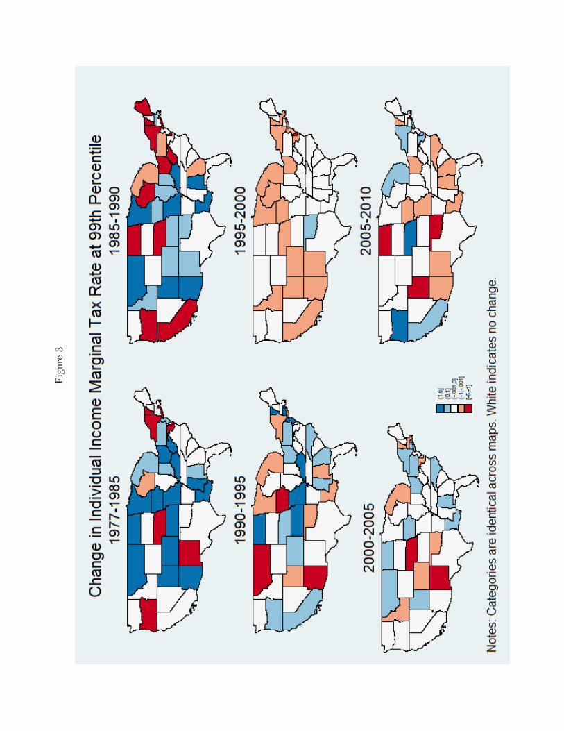
Figure
3

Figure
4

Figure
5

Figure
6
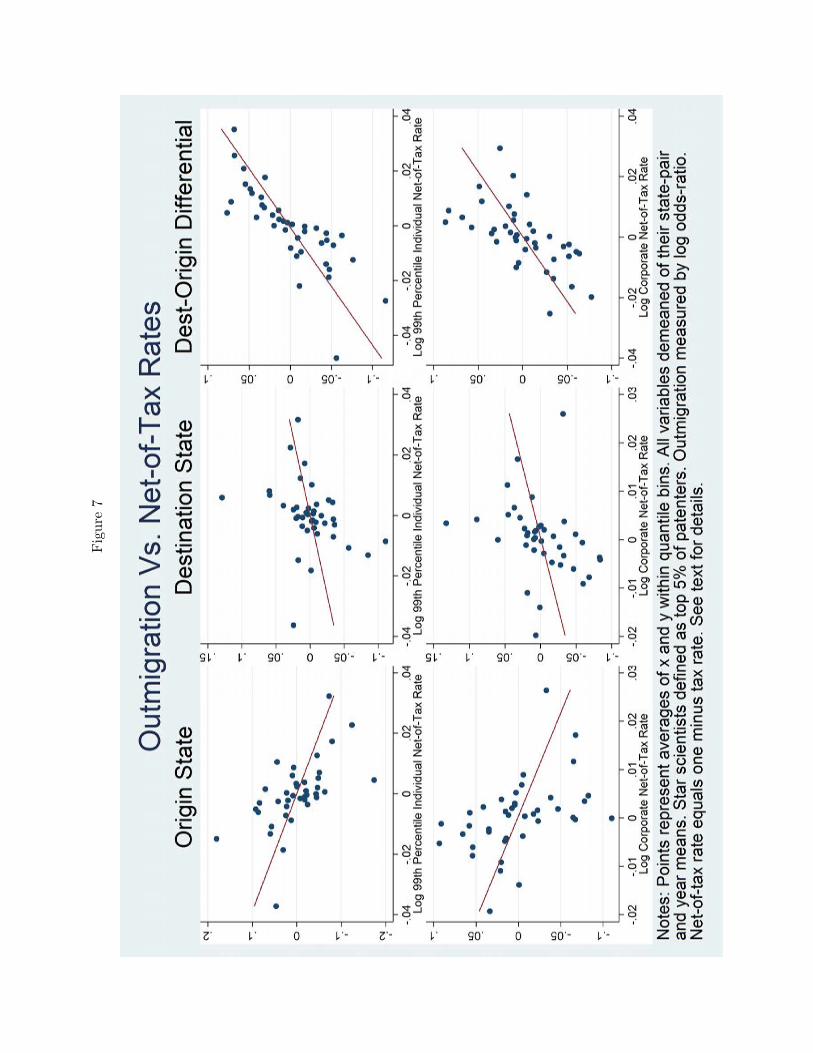
Figure
7

Figure 8
-10
-50
510
-10 -5 0 5 10Horizon (Years Ahead)
1-year Net-of-Tax Change
-4-2
02
46
-10 -5 0 5 10Horizon (Years Ahead)
3-year Net-of-Tax Change
-4-2
02
46
-10 -5 0 5 10Horizon (Years Ahead)
5-year Net-of-Tax Change
Brackets indicate 95% and 90% confidence intervals. Dashed red lines indicate start and end of treatmentperiod. Observations weighted by average annual outflow for each dyad. All regressions use a commonsample (observations available for 10 year horizon). Regression include region-pair*year fixed effects.
Impulse Response to Individual MTR Net-of-Tax Change
Figure 9
-50
510
-10 -5 0 5 10Horizon (Years Ahead)
1-year Net-of-Tax Change
-50
5
-10 -5 0 5 10Horizon (Years Ahead)
3-year Net-of-Tax Change
-4-2
02
46
-10 -5 0 5 10Horizon (Years Ahead)
5-year Net-of-Tax Change
Brackets indicate 95% and 90% confidence intervals. Dashed red lines indicate start and end of treatmentperiod. Observations weighted by average annual outflow for each dyad. All regressions use a commonsample (observations available for 10 year horizon). Regression include region-pair*year fixed effects.
Impulse Response to CIT Net-of-Tax Change

Figure 10
-50
510
-10 -5 0 5 10Horizon (Years Ahead)
1-year Net-of-Tax Change
-4-2
02
46
-10 -5 0 5 10Horizon (Years Ahead)
3-year Net-of-Tax Change
-20
24
68
-10 -5 0 5 10Horizon (Years Ahead)
5-year Net-of-Tax Change
Brackets indicate 95% and 90% confidence intervals. Dashed red lines indicate start and end of treatmentperiod. Observations weighted by average annual outflow for each dyad. All regressions use a commonsample (observations available for 10 year horizon). Regression include region-pair*year fixed effects.
Impulse Response to Investment Credit Net-of-Tax Change
Figure 11
-4-2
02
4
-10 -5 0 5 10Horizon (Years Ahead)
1-year Net-of-Tax Change
-2-1
01
2
-10 -5 0 5 10Horizon (Years Ahead)
3-year Net-of-Tax Change
-10
12
3
-10 -5 0 5 10Horizon (Years Ahead)
5-year Net-of-Tax Change
Brackets indicate 95% and 90% confidence intervals. Dashed red lines indicate start and end of treatmentperiod. Observations weighted by average annual outflow for each dyad. All regressions use a commonsample (observations available for 10 year horizon). Regression include region-pair*year fixed effects.
Impulse Response to R&D credit Net-of-Tax Change

Table A1: Summary Statistics over 51 states-Star Population, 99th Perc. MTR, and Corp. Income Tax
Pop Star 95 Pop Star 95 99th Perc. MTR 99th Perc. MTR CIT CIT(1) (2) (3) (4) (5) (6)
2006 value 1977-2006 %-change 2006 value 1977-2006 %-change 2006 value 1977-2006 %-changeAlabama 26 -0.5667 0.0360 1.2360 0.0650 0.3000Alaska 0 -1 0 -1 0.0940 0.0000Arizona 267 1.3421 0.0466 0.7719 0.0697 -0.3362Arkansas 10 0 0.0700 0 0.0650 0.0833California 3869 1.8852 0.0930 -0.1545 0.0884 -0.0178Colorado 192 0.3617 0.0463 0.8821 0.0463 -0.0740Connecticut 290 -0.1667 0.0500 -1 0.0750 -0.2500Delaware 77 -0.4539 0.0595 -0.6995 0.0870 0.0000DC 7 -0.3000 0.0870 -0.1230 0.0998 0.0081Florida 238 0.1174 0 -1 0.0550 0.1000Georgia 174 1.2308 0.0577 -0.0383 0.0600 0.0000Hawaii 10 0.4286 0.0778 -0.2157 0.0640 -0.0054Idaho 219 20.9000 0.0780 0.0400 0.0760 0.1692Illinois 419 -0.5117 0.0300 0.2000 0.0730 0.8250Indiana 129 -0.4921 0.0340 0.7000 0.0850 0.4167Iowa 82 0.1549 0.0647 0.4410 0.1200 0.2000Kansas 41 -0.2115 0.0645 1.1644 0.0735 0.0889Kentucky 60 -0.2208 0.0600 2.0928 0.0700 0.2069Louisiana 24 -0.6800 0.0432 1.2979 0.0800 0.0000Maine 14 0.0769 0.0850 -0.1500 0.0893 0.2757Maryland 154 -0.2261 0.0475 -0.3667 0.0700 0.0000Massachusetts 645 0.2697 0.0530 -0.0130 0.0950 0.0000Michigan 470 -0.1826 0.0390 -0.1522 0.0190 -0.1915Minnesota 593 2.1711 0.0785 0.5067 0.0980 -0.1833Mississippi 12 -0.0769 0.0500 0.6234 0.0500 0.2500Missouri 99 -0.3694 0.0600 2.0769 0.0625 0.2500Montana 5 -0.2857 0.0690 0.6788 0.0675 0.0000Nebraska 31 -0.1389 0.0509 -0.5402 0.0781 0.5778Nevada 44 2.1429 0 -1 0 -1.0000New Hampshire 66 0.9412 0 -1 0.0925 0.1562New Jersey 605 -0.4271 0.0637 1.5480 0.0900 0.2000New Mexico 40 1.2222 0.0530 -0.4111 0.0760 0.5200New York 1265 0.2199 0.0685 -0.5433 0.0750 -0.2500North Carolina 327 1.5349 0.0825 0.1786 0.0690 0.1500North Dakota 5 0.2500 0.0535 0.8385 0.0700 0.1667Ohio 398 -0.4033 0.0687 0.9629 0.0850 0.0625Oklahoma 86 -0.5635 0.0636 0.1237 0.0600 0.5000Oregon 291 4.1964 0.0900 -0.3077 0.0660 -0.0571Pennsylvania 502 -0.3597 0.0307 0.5350 0.0999 0.0516Rhode Island 33 0.1000 0.0920 -0.2042 0.0900 0.1250South Carolina 59 0.0727 0.0700 0 0.0500 -0.1667South Dakota 2 0 0 -1 0 -1.0000Tennessee 91 0.0706 0 -1 0.0650 0.0833Texas 956 1.0297 0 -1 0.0450 0.0588Utah 84 0.7500 0.0600 1.3622 0.0500 0.2500Vermont 163 7.5789 0.0843 -0.4304 0.0975 0.3000Virginia 95 -0.2857 0.0575 0 0.0600 0.0000Washington 535 4.4592 0 -1 0 -1.0000West Virginia 4 -0.8750 0.0650 -0.2216 0.0900 0.5000Wisconsin 216 0.0588 0.0675 -0.3415 0.0790 0.0000Wyoming 3 -0.4000 0 -1 0 -1.0000

Table A2: Baseline Specification, Top 1% Stars
(1) (2) (3) (4) (5) (6) (7) (8)MTR, 99.9th Perc. -3.4097∗∗∗ 4.4365∗∗∗ 4.4942∗∗∗ 3.2041∗∗∗ 4.4461∗∗∗ 3.2277∗∗∗ 1.6859∗∗ 7.8390∗∗∗
(0.7841) (0.6364) (0.6477) (0.5808) (0.7304) (0.6012) (0.7862) (1.5922)
MTR, 99th Perc. -3.2499∗∗∗ 4.3348∗∗∗ 4.3645∗∗∗ 3.1874∗∗∗ 4.2400∗∗∗ 3.1538∗∗∗ 2.0446∗∗ 7.3936∗∗∗
(0.7947) (0.6239) (0.6319) (0.5781) (0.7157) (0.6036) (0.7948) (1.6529)
MTR, 95th Perc. -3.2926∗∗∗ 4.4616∗∗∗ 4.3895∗∗∗ 3.2730∗∗∗ 4.3060∗∗∗ 3.3071∗∗∗ 2.0229∗∗ 7.8764∗∗∗
(0.7991) (0.6257) (0.6314) (0.5883) (0.7250) (0.6240) (0.8085) (1.6343)
State CIT Rate -6.3729∗∗∗ 3.4329∗∗∗ 3.4581∗∗∗ 3.5716∗∗∗ 2.9124∗∗∗ 2.8817∗∗∗ 1.4807 8.0372∗∗∗
(0.7385) (0.9647) (0.9082) (0.9330) (1.0680) (1.0400) (0.9942) (2.1419)
State ITC 8.6758∗∗∗ 1.7791∗∗∗ 1.6382∗∗ 0.7456 1.5666∗∗ 0.6440 2.3159∗∗ 1.6069(1.5858) (0.6259) (0.6526) (0.6742) (0.6759) (0.6078) (1.1272) (1.1791)
R&D Credit 4.8045∗∗∗ 0.7599∗∗∗ 0.6661∗∗ -0.3163 0.4245 -0.7682∗∗∗ 0.9533∗∗ -0.2909(0.7416) (0.2590) (0.2683) (0.2869) (0.3131) (0.2916) (0.4169) (0.6390)
Origin, Destination State FE No Yes No No No No No No
Origin*Destination Pair FE No No Yes Yes Yes Yes Yes Yes
Origin Region*Year FE No No No Yes No No No No
Destination Region*Year FE No No No No Yes No No No
Origin & Destination PairRegion*Year FE No No No No No Yes No No
Origin State*Year FE No No No No No No Yes No
Destination State*Year FE No No No No No No No Yes
Each entry is from a separate regression. Coefficients are estimates of η or η′ from equation (3). ∗ p < 0.10, ∗∗ p < 0.05, ∗∗∗ p < 0.01
Standard errors in parentheses, with two-way clustering by origin-state*year and destination-state*year.
All regressions include year fixed effects, and have 6258 observations
Table A3: Baseline Specification, Top 10% Stars
(1) (2) (3) (4) (5) (6) (7) (8)MTR, 99.9th Perc. -2.3282∗∗∗ 2.8865∗∗∗ 2.6450∗∗∗ 1.8764∗∗∗ 2.6389∗∗∗ 1.8190∗∗∗ 1.3685∗∗ 4.0279∗∗∗
(0.6409) (0.4873) (0.4875) (0.4369) (0.5238) (0.4113) (0.6239) (0.9179)
MTR, 99th Perc. -2.1263∗∗∗ 2.7985∗∗∗ 2.5204∗∗∗ 1.8051∗∗∗ 2.4699∗∗∗ 1.7194∗∗∗ 1.4130∗∗ 3.7147∗∗∗
(0.6417) (0.4850) (0.4892) (0.4446) (0.5206) (0.4133) (0.6466) (0.9221)
MTR, 95th Perc. -2.1916∗∗∗ 2.7768∗∗∗ 2.4730∗∗∗ 1.7309∗∗∗ 2.4411∗∗∗ 1.6615∗∗∗ 1.3979∗∗ 3.7618∗∗∗
(0.6464) (0.4915) (0.4956) (0.4562) (0.5294) (0.4264) (0.6656) (0.9368)
State CIT Rate -5.3547∗∗∗ 1.9887∗∗∗ 1.8812∗∗∗ 1.7847∗∗∗ 1.0311 0.8871 2.5883∗∗∗ 1.4481(0.6411) (0.6858) (0.6649) (0.5951) (0.7540) (0.6142) (0.7112) (1.2771)
State ITC 6.0969∗∗∗ 1.7086∗∗∗ 1.7025∗∗∗ 1.4818∗∗∗ 1.6679∗∗∗ 1.4892∗∗∗ 2.3795∗∗∗ 1.1091(1.2981) (0.4011) (0.4563) (0.5312) (0.4152) (0.4532) (0.8894) (0.6746)
R&D Credit 4.2379∗∗∗ 0.3990∗∗ 0.3861∗∗ 0.0102 0.0553 -0.3934∗∗ 1.2568∗∗∗ -0.6651∗
(0.5769) (0.1732) (0.1826) (0.2043) (0.1843) (0.1816) (0.3018) (0.3397)Origin, Destination State FE No Yes No No No No No No
Origin*Destination Pair FE No No Yes Yes Yes Yes Yes Yes
Origin Region*Year FE No No No Yes No No No No
Destination Region*Year FE No No No No Yes No No No
Origin & Destination PairRegion*Year FE No No No No No Yes No No
Origin State*Year FE No No No No No No Yes No
Destination State*Year FE No No No No No No No Yes
Each entry is from a separate regression. Coefficients are estimates of η or η′ from equation (3). ∗ p < 0.10, ∗∗ p < 0.05, ∗∗∗ p < 0.01
Standard errors in parentheses, with two-way clustering by origin-state*year and destination-state*year.
All regressions include year fixed effects, and have 14193 observations

Table A4: Baseline Specification, Stars Based on Citations
(1) (2) (3) (4) (5) (6) (7) (8)MTR, 99.9th Perc. -2.8062∗∗∗ 3.5170∗∗∗ 3.5874∗∗∗ 2.2380∗∗∗ 3.6387∗∗∗ 2.0963∗∗∗ 2.1424∗∗ 5.3159∗∗∗
(0.7421) (0.6151) (0.6419) (0.6052) (0.6715) (0.5654) (0.9127) (1.0221)
MTR, 99th Perc. -2.5900∗∗∗ 3.3103∗∗∗ 3.3489∗∗∗ 2.1207∗∗∗ 3.3402∗∗∗ 1.9560∗∗∗ 2.2577∗∗ 4.7843∗∗∗
(0.7470) (0.6148) (0.6588) (0.6320) (0.6854) (0.5842) (0.9417) (1.0911)
MTR, 95th Perc. -2.6676∗∗∗ 3.1548∗∗∗ 3.1070∗∗∗ 1.9681∗∗∗ 3.1665∗∗∗ 1.9143∗∗∗ 1.9387∗∗ 4.6831∗∗∗
(0.7523) (0.6012) (0.6396) (0.6204) (0.6740) (0.5806) (0.9220) (1.0741)
State CIT Rate -5.2704∗∗∗ 1.8121∗∗ 1.9413∗∗∗ 1.8564∗∗∗ 1.1658 0.9763 2.4371∗∗∗ 1.2923(0.6827) (0.7431) (0.6969) (0.6454) (0.7810) (0.6674) (0.8342) (1.4300)
State ITC 6.8684∗∗∗ 1.8639∗∗∗ 1.9298∗∗∗ 1.6794∗∗∗ 1.8376∗∗∗ 1.5761∗∗∗ 2.6185∗∗∗ 1.4780∗∗
(1.4039) (0.4442) (0.4947) (0.5446) (0.4493) (0.4499) (0.9349) (0.6718)
R&D Credit 4.3838∗∗∗ 0.4728∗∗ 0.4619∗∗ 0.0210 0.1648 -0.3147 1.1870∗∗∗ -0.4950(0.6124) (0.1952) (0.2034) (0.2234) (0.2054) (0.1988) (0.3386) (0.3866)
Origin, Destination State FE No Yes No No No No No No
Origin*Destination Pair FE No No Yes Yes Yes Yes Yes Yes
Origin Region*Year FE No No No Yes No No No No
Destination Region*Year FE No No No No Yes No No No
Origin & Destination PairRegion*Year FE No No No No No Yes No No
Origin State*Year FE No No No No No No Yes No
Destination State*Year FE No No No No No No No Yes
Each entry is from a separate regression. Coefficients are estimates of η or η′ from equation (3). ∗ p < 0.10, ∗∗ p < 0.05, ∗∗∗ p < 0.01
Standard errors in parentheses, with two-way clustering by origin-state*year and destination-state*year.
All regressions include year fixed effects, and have 10991 observations
Table A5: Baseline Specification, Avg. State Tax Rates
(1) (2) (3) (4) (5) (6) (7) (8)MTR, 99.9th Perc. -3.4203∗∗∗ 3.0427∗∗∗ 3.0566∗∗∗ 2.6189∗∗∗ 2.9757∗∗∗ 2.4588∗∗∗ 2.0374∗∗∗ 3.6879∗∗∗
(0.7450) (0.5623) (0.5714) (0.4987) (0.6107) (0.4812) (0.6552) (1.1148)
MTR, 99th Perc. -2.4697∗∗∗ 3.6649∗∗∗ 3.5778∗∗∗ 2.8159∗∗∗ 3.4382∗∗∗ 2.5591∗∗∗ 2.4172∗∗∗ 4.6317∗∗∗
(0.7497) (0.6060) (0.6233) (0.5373) (0.6619) (0.5065) (0.7428) (1.2248)
MTR, 95th Perc. -1.0825 5.0735∗∗∗ 4.9366∗∗∗ 3.6108∗∗∗ 4.6578∗∗∗ 3.1408∗∗∗ 3.5748∗∗∗ 6.4391∗∗∗
(0.7429) (0.6960) (0.7161) (0.6133) (0.7536) (0.5662) (0.8918) (1.3968)Origin, Destination State FE No Yes No No No No No No
Origin*Destination Pair FE No No Yes Yes Yes Yes Yes Yes
Origin Region*Year FE No No No Yes No No No No
Destination Region*Year FE No No No No Yes No No No
Origin & Destination PairRegion*Year FE No No No No No Yes No No
Origin State*Year FE No No No No No No Yes No
Destination State*Year FE No No No No No No No Yes
Each entry is from a separate regression. Coefficients are estimates of η or η′ from equation (3). ∗ p < 0.10, ∗∗ p < 0.05, ∗∗∗ p < 0.01
Standard errors in parentheses, with two-way clustering by origin-state*year and destination-state*year.
All regressions include year fixed effects, and have 11941 observations

Appendix
Figure
1

Appendix
Figure
2