The effect of observables, functional specifications, modelfeatures and shocks on identification in linearized DSGE

models

Sergey Ivashchenkoa,b,c,d, Willi Mutschlere,∗

aThe Institute of Regional Economy Problems, Russian Academy of Sciences, Russia.bFinancial Research Institute, Ministry of Finance, Russia.

cThe faculty of Economics, Saint-Petersburg State University, Russia.dNational Research University Higher School of Economics, St. Petersburg, Russia.

eCenter for Quantitative Economics, University of Munster, Am Stadtgraben 9, 48143 Munster,Germany.

Abstract

Both the investment adjustment costs parameters in Kim (2003) and the monetary policy

rule parameters in An & Schorfheide (2007) are locally not identifiable. We show means

to dissolve this theoretical lack of identification by looking at (1) the set of observed

variables, (2) functional specifications (level vs. growth costs, output-gap definition),

(3) model features (capital utilization, partial inflation indexation), and (4) additional

shocks (investment-specific technology, preference). Moreover, we discuss the effect of

these changes on the strength of parameter identification from a Bayesian point of view.

Our results indicate that researchers should treat parameter identification as a model

property, i.e. from a model building perspective.

Keywords: identification, weak identification, investment adjustment costs, Taylor rule,

model features, shocks

JEL: C18, C51, C68, E22, E52

?The authors thank Jan Capek, Jinill Kim, Ludger Linnemann, Ales Marsal, Marco Ratto, MarkTrede and Bernd Wilfling for helpful comments. This paper was presented at the Young EconomistsMeeting Brno, the 8th Conference on Growth and Business Cycles in Theory and Practice Manchester,and the 2018 Course on Identification and Global Sensitivity Analysis in Ispra.??The second author acknowledges financial support from the Deutsche Forschungsgemeinschaft

through Grant No. 411754673. The usual disclaimer applies.∗Corresponding author.Email addresses: sergey.ivashchenko.ru@gmail.com (Sergey Ivashchenko), willi@mutschler.eu

(Willi Mutschler)Preprint submitted to May 28, 2019

1. Introduction

The identification problem in DSGE models. DSGE models have become a major toolkit

for empirical macroeconomic research and an important policy tool used in central banks.

Many different methods of solving and estimating DSGE models have been developed

and used in order to obtain a detailed analysis and thorough estimation of dynamic

macroeconomic relationships, see e.g. Fernandez-Villaverde et al. (2016). Recently, the

question of identifiability of DSGE models has proven to be of major importance, espe-

cially since the identification of a model precedes (consistent) estimation and inference of

an unknown parameter vector θ ∈ Θ from observations Y . θ0 is said to be globally iden-

tified if for the family of probability distributions p(Y |θ) generated by a DSGE model:

p(Y |θ) = p(Y |θ0) implies θ = θ0. If this condition is only satisfied for values of θ in an

open neighborhood of θ0, then θ0 is said to be locally identified. From an economet-

ric point of view, local identification belongs to the usual regularity conditions and is

necessary for the asymptotic theory of e.g. maximum likelihood estimation. From an

economic point of view, lack of identification leads to wrong conclusions from calibration,

estimation and inference (Canova & Sala, 2009), whereas the source of identification in-

fluences empirical findings (Rıos-Rull et al., 2012). Accordingly, experience shows that

it is quite difficult both for Frequentist as well as Bayesian researchers to maximize

the likelihood/posterior or minimize some (moment) objective function, because these

functions are typically not well behaved as one has to deal with multiple local extrema,

weak curvature in some directions of the parameter space and ridges. The evaluation of

first-order and second-order derivatives is intractable and gradient based optimization

methods perform quite poorly (Andreasen, 2010). The resulting estimators may often

lie on the boundary of the theoretically admissible parameter space and conventional

Gaussian asymptotics yield poor approximations to the true sampling distribution. In

many cases the source of these particular outcomes is due to local or weak identifiability

issues or an unfortunate choice of observables. Nevertheless, in particular Bayesian (and

to some extent also Frequentist) estimation of DSGE models has rapidly progressed;

however, the study of identifiability, which should precede estimation, is still a rather

neglected topic for applied macroeconomists.

1

Research question. In this paper we seek to answer the question whether researchers

should treat parameter identification as a model property, i.e. from a model building

perspective. To this end, we revisit the linearized models of Kim (2003) and An &

Schorfheide (2007), as it is well-known that both the multisectoral and intertemporal

investment adjustment costs parameters in Kim (2003) and the monetary policy rule

parameters in An & Schorfheide (2007) are locally not identifiable (Mutschler, 2016;

Ratto & Iskrev, 2011). We try to dissolve this theoretical lack of identifiability by looking

at (1) the set of observed variables, (2) functional specifications, (3) model features, and

(4) additional shocks. Moreover, we discuss the effect of these changes on the strength

of parameter identification from a Bayesian point of view.

Research methods. Regarding (1), we complement Canova et al. (2014) by selecting ob-

servables in a way that optimizes parameter identification. To this end, we are agnostic

and analyze local identification for all possible combinations of observable variables. For

(2), we focus on the functional specification of the intertemporal investment adjustment

costs in the Kim (2003) model and of the output gap in the monetary policy rule of the

An & Schorfheide (2007) model. With respect to (3), we analyze the effect on identifica-

tion of capital utilization in the first model and of a partial inflation indexation scheme

in the second model. Lastly regarding (4), we add an investment-specific technological

shock into the former and a preference shock on the discount factor into the latter model.

Our focus lies both on the theoretical properties as well as the strength of identification

of the model parameters in linearized DSGE models. To this end, we solve the model

using first-order perturbation techniques and carefully check the rank criteria of Iskrev

(2010), Komunjer & Ng (2011) and Qu & Tkachenko (2012) for all considered model

variants and observables. Regarding the strength of identification we make use of Koop

et al. (2013)’s Bayesian learning rate indicator.

Outline. In section 2, we summarize our implementation of the used tools to check for

parameter identification in linearized DSGE models. We analyze the identification prop-

erties of the Kim (2003) model in section 3, whereas section 4 provides the corresponding

analysis for the An & Schorfheide (2007) model. In section 5, we discuss our results from

a model building perspective. Section 6 concludes. The replication files are available in

2

a GitHub repository (https://github.com/wmutschl/identification-note/).

2. Implementation of identification checks

Rank checks. We check the local identification properties according to Iskrev (2010),

Komunjer & Ng (2011) and Qu & Tkachenko (2012) with Dynare (Adjemian et al.,

2011). In a nutshell, Iskrev (2010)’s approach to find non-identified parameters is based

on observational equivalent moments, i.e. on the sensitivity of the theoretical mean and

autocovariances, whereas Qu & Tkachenko (2012)’s approach focuses on observational

equivalent spectral properties, i.e. on the sensitivity of the theoretical mean and spec-

trum of observables. Komunjer & Ng (2011) study the implications of observational

equivalence in minimal systems and derive a finite system of nonlinear equations that

admits a unique solution if and only if the parameters are identified. In all three cases,

we need to compute Jacobians w.r.t the model parameters and check whether these have

full rank. Iskrev (2010) follows an analytical approach to compute the Jacobian of mo-

ments using Kronecker products, which is extended in Ratto & Iskrev (2011) by making

use of computationally more efficient generalized Sylvester equations. Both Komunjer

& Ng (2011) and Qu & Tkachenko (2012), however, rely on numerical methods to com-

pute the derivatives of the minimal system and spectrum, which is known to be sensitive

to the thresholds and tolerance levels used. We are, however, able to extend the ideas

from Iskrev (2010) and Ratto & Iskrev (2011) to also compute these Jacobians analyti-

cally. Hence, we extend the identification toolbox of Dynare such that users are able to

compute all three rank criteria (moments, minimal system or spectrum) analytically (by

either using Kronecker products or generalized Sylvester equations).1 To pinpoint the

problematic parameters that yield rank failure, the default in Dynare is to look into the

nullspace and evaluate multicorrelation coefficients of the columns. Another (numerically

more robust) approach, which is contributed to the software and used in this paper, is to

check the ranks for all possible combinations of parameters, and to mark the ones that

do not pass the rank check.

1Our contributions and improvements are already merged into the 4.6-unstable branch. For morecomputational details, see the merge request (Mutschler, 2019).

3

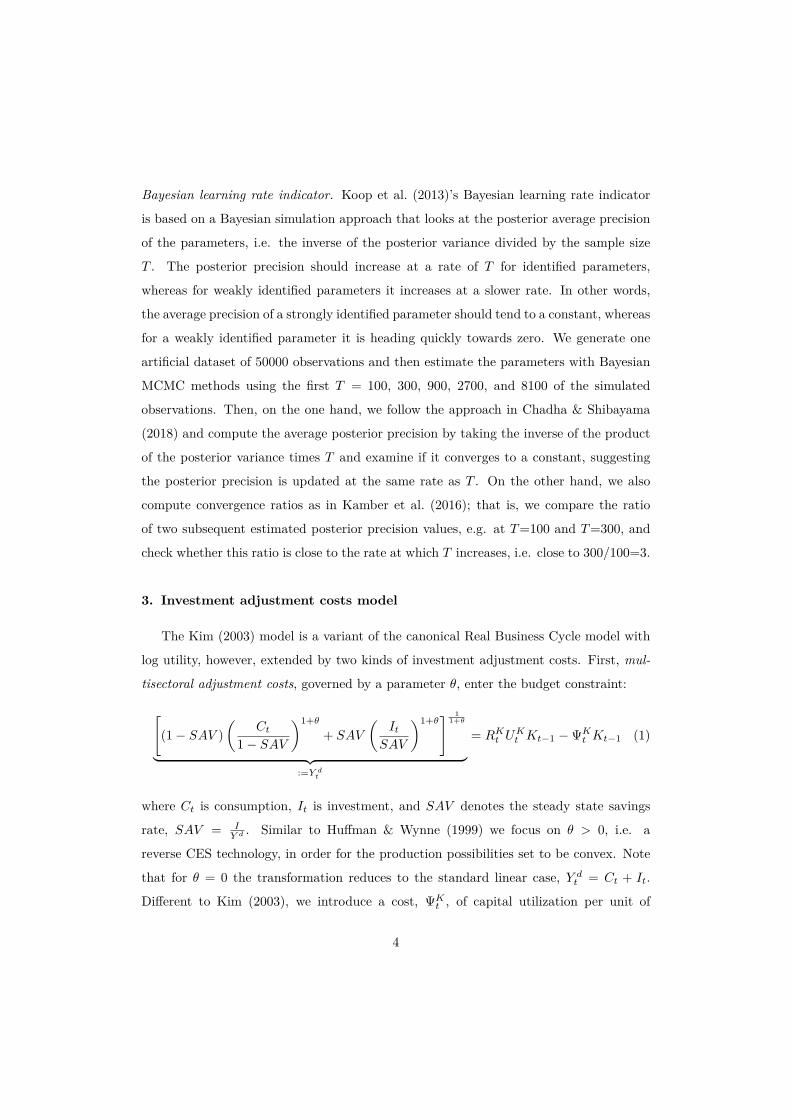
Bayesian learning rate indicator. Koop et al. (2013)’s Bayesian learning rate indicator

is based on a Bayesian simulation approach that looks at the posterior average precision

of the parameters, i.e. the inverse of the posterior variance divided by the sample size

T . The posterior precision should increase at a rate of T for identified parameters,

whereas for weakly identified parameters it increases at a slower rate. In other words,

the average precision of a strongly identified parameter should tend to a constant, whereas

for a weakly identified parameter it is heading quickly towards zero. We generate one

artificial dataset of 50000 observations and then estimate the parameters with Bayesian

MCMC methods using the first T = 100, 300, 900, 2700, and 8100 of the simulated

observations. Then, on the one hand, we follow the approach in Chadha & Shibayama

(2018) and compute the average posterior precision by taking the inverse of the product

of the posterior variance times T and examine if it converges to a constant, suggesting

the posterior precision is updated at the same rate as T . On the other hand, we also

compute convergence ratios as in Kamber et al. (2016); that is, we compare the ratio

of two subsequent estimated posterior precision values, e.g. at T=100 and T=300, and

check whether this ratio is close to the rate at which T increases, i.e. close to 300/100=3.

3. Investment adjustment costs model

The Kim (2003) model is a variant of the canonical Real Business Cycle model with

log utility, however, extended by two kinds of investment adjustment costs. First, mul-

tisectoral adjustment costs, governed by a parameter θ, enter the budget constraint:

[(1− SAV )

(Ct

1− SAV

)1+θ+ SAV

(It

SAV

)1+θ] 1

1+θ

︸ ︷︷ ︸:=Y dt

= RKt UKt Kt−1 −ΨK

t Kt−1 (1)

where Ct is consumption, It is investment, and SAV denotes the steady state savings

rate, SAV = IY d

. Similar to Huffman & Wynne (1999) we focus on θ > 0, i.e. a

reverse CES technology, in order for the production possibilities set to be convex. Note

that for θ = 0 the transformation reduces to the standard linear case, Y dt = Ct + It.

Different to Kim (2003), we introduce a cost, ΨKt , of capital utilization per unit of

4

physical capital.2 UKt denotes the capital utilization rate and physical (end-of-period)

capital, Kt, is transformed into effective (end-of-period) capital, Kst , according to Ks

t−1 =

UKt Kt−1. Effective capital is then rented to the representative firm at the gross rental

rate RKt . The firm produces a homogeneous good using a Cobb-Douglas production

function, Yt = At(Kst−1)α, where At denotes total factor productivity.

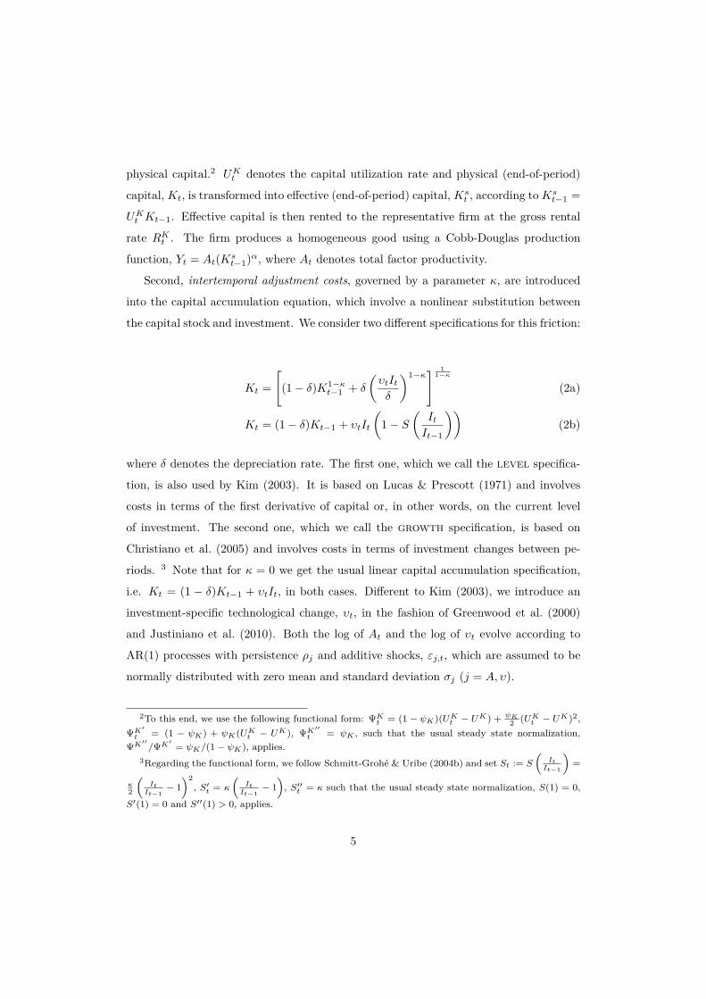
Second, intertemporal adjustment costs, governed by a parameter κ, are introduced

into the capital accumulation equation, which involve a nonlinear substitution between

the capital stock and investment. We consider two different specifications for this friction:

Kt =[

(1− δ)K1−κt−1 + δ

(υtItδ

)1−κ] 1

1−κ

(2a)

Kt = (1− δ)Kt−1 + υtIt

(1− S

(ItIt−1

))(2b)

where δ denotes the depreciation rate. The first one, which we call the level specifica-

tion, is also used by Kim (2003). It is based on Lucas & Prescott (1971) and involves

costs in terms of the first derivative of capital or, in other words, on the current level

of investment. The second one, which we call the growth specification, is based on

Christiano et al. (2005) and involves costs in terms of investment changes between pe-

riods. 3 Note that for κ = 0 we get the usual linear capital accumulation specification,

i.e. Kt = (1 − δ)Kt−1 + υtIt, in both cases. Different to Kim (2003), we introduce an

investment-specific technological change, υt, in the fashion of Greenwood et al. (2000)

and Justiniano et al. (2010). Both the log of At and the log of υt evolve according to

AR(1) processes with persistence ρj and additive shocks, εj,t, which are assumed to be

normally distributed with zero mean and standard deviation σj (j = A, υ).

2To this end, we use the following functional form: ΨKt = (1− ψK)(UKt − UK) + ψK2 (UKt − UK)2,

ΨK′t = (1 − ψK) + ψK(UKt − UK), ΨK′′t = ψK , such that the usual steady state normalization,ΨK′′/ΨK′ = ψK/(1− ψK), applies.

3Regarding the functional form, we follow Schmitt-Grohe & Uribe (2004b) and set St := S

(ItIt−1

)=

κ2

(ItIt−1

− 1)2

, S′t = κ

(ItIt−1

− 1)

, S′′t = κ such that the usual steady state normalization, S(1) = 0,

S′(1) = 0 and S′′(1) > 0, applies.

5

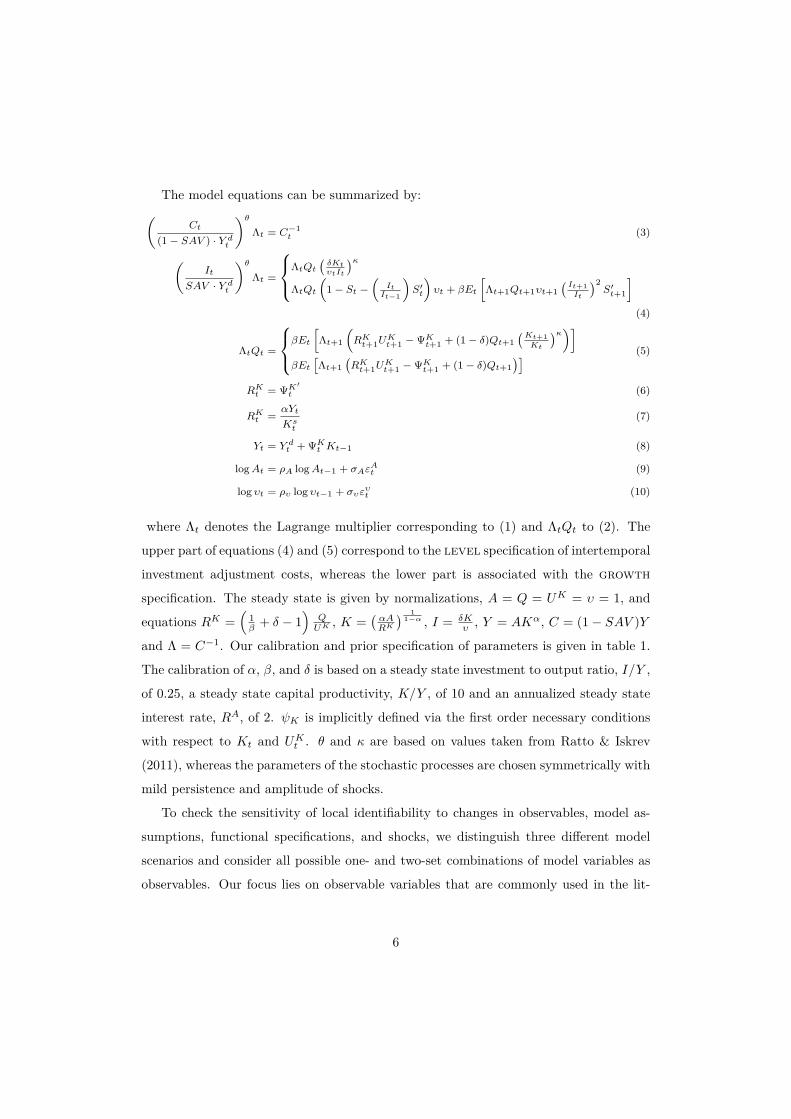
The model equations can be summarized by:(Ct

(1− SAV ) · Y dt

)θΛt = C−1

t (3)

(It

SAV · Y dt

)θΛt =

ΛtQt(δKtυtIt

)κΛtQt

(1− St −

(ItIt−1

)S′t

)υt + βEt

[Λt+1Qt+1υt+1

(It+1It

)2S′t+1

](4)

ΛtQt =

βEt[

Λt+1

(RKt+1U

Kt+1 −ΨKt+1 + (1− δ)Qt+1

(Kt+1Kt

)κ)]βEt

[Λt+1

(RKt+1U

Kt+1 −ΨKt+1 + (1− δ)Qt+1

)] (5)

RKt = ΨK′

t (6)

RKt =αYt

Kst

(7)

Yt = Y dt + ΨKt Kt−1 (8)

logAt = ρA logAt−1 + σAεAt (9)

log υt = ρυ log υt−1 + συευt (10)

where Λt denotes the Lagrange multiplier corresponding to (1) and ΛtQt to (2). The

upper part of equations (4) and (5) correspond to the level specification of intertemporal

investment adjustment costs, whereas the lower part is associated with the growth

specification. The steady state is given by normalizations, A = Q = UK = υ = 1, and

equations RK =(

1β + δ − 1

)QUK

, K =(αARK

) 11−α , I = δK

υ , Y = AKα, C = (1− SAV )Y

and Λ = C−1. Our calibration and prior specification of parameters is given in table 1.

The calibration of α, β, and δ is based on a steady state investment to output ratio, I/Y ,

of 0.25, a steady state capital productivity, K/Y , of 10 and an annualized steady state

interest rate, RA, of 2. ψK is implicitly defined via the first order necessary conditions

with respect to Kt and UKt . θ and κ are based on values taken from Ratto & Iskrev

(2011), whereas the parameters of the stochastic processes are chosen symmetrically with

mild persistence and amplitude of shocks.

To check the sensitivity of local identifiability to changes in observables, model as-

sumptions, functional specifications, and shocks, we distinguish three different model

scenarios and consider all possible one- and two-set combinations of model variables as

observables. Our focus lies on observable variables that are commonly used in the lit-

6

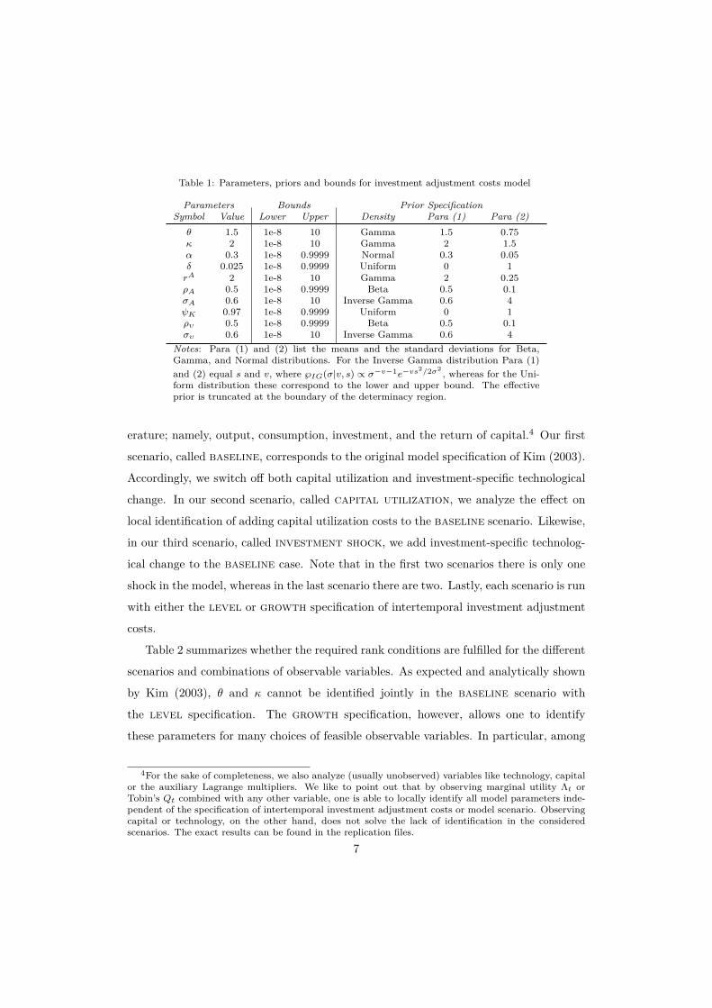
Table 1: Parameters, priors and bounds for investment adjustment costs model

Parameters Bounds Prior SpecificationSymbol Value Lower Upper Density Para (1) Para (2)

θ 1.5 1e-8 10 Gamma 1.5 0.75κ 2 1e-8 10 Gamma 2 1.5α 0.3 1e-8 0.9999 Normal 0.3 0.05δ 0.025 1e-8 0.9999 Uniform 0 1rA 2 1e-8 10 Gamma 2 0.25ρA 0.5 1e-8 0.9999 Beta 0.5 0.1σA 0.6 1e-8 10 Inverse Gamma 0.6 4ψK 0.97 1e-8 0.9999 Uniform 0 1ρυ 0.5 1e-8 0.9999 Beta 0.5 0.1συ 0.6 1e-8 10 Inverse Gamma 0.6 4

Notes: Para (1) and (2) list the means and the standard deviations for Beta,Gamma, and Normal distributions. For the Inverse Gamma distribution Para (1)and (2) equal s and v, where ℘IG(σ|v, s) ∝ σ−v−1e−vs

2/2σ2 , whereas for the Uni-form distribution these correspond to the lower and upper bound. The effectiveprior is truncated at the boundary of the determinacy region.

erature; namely, output, consumption, investment, and the return of capital.4 Our first

scenario, called baseline, corresponds to the original model specification of Kim (2003).

Accordingly, we switch off both capital utilization and investment-specific technological

change. In our second scenario, called capital utilization, we analyze the effect on

local identification of adding capital utilization costs to the baseline scenario. Likewise,

in our third scenario, called investment shock, we add investment-specific technolog-

ical change to the baseline case. Note that in the first two scenarios there is only one

shock in the model, whereas in the last scenario there are two. Lastly, each scenario is run

with either the level or growth specification of intertemporal investment adjustment

costs.

Table 2 summarizes whether the required rank conditions are fulfilled for the different

scenarios and combinations of observable variables. As expected and analytically shown

by Kim (2003), θ and κ cannot be identified jointly in the baseline scenario with

the level specification. The growth specification, however, allows one to identify

these parameters for many choices of feasible observable variables. In particular, among

4For the sake of completeness, we also analyze (usually unobserved) variables like technology, capitalor the auxiliary Lagrange multipliers. We like to point out that by observing marginal utility Λt orTobin’s Qt combined with any other variable, one is able to locally identify all model parameters inde-pendent of the specification of intertemporal investment adjustment costs or model scenario. Observingcapital or technology, on the other hand, does not solve the lack of identification in the consideredscenarios. The exact results can be found in the replication files.

7

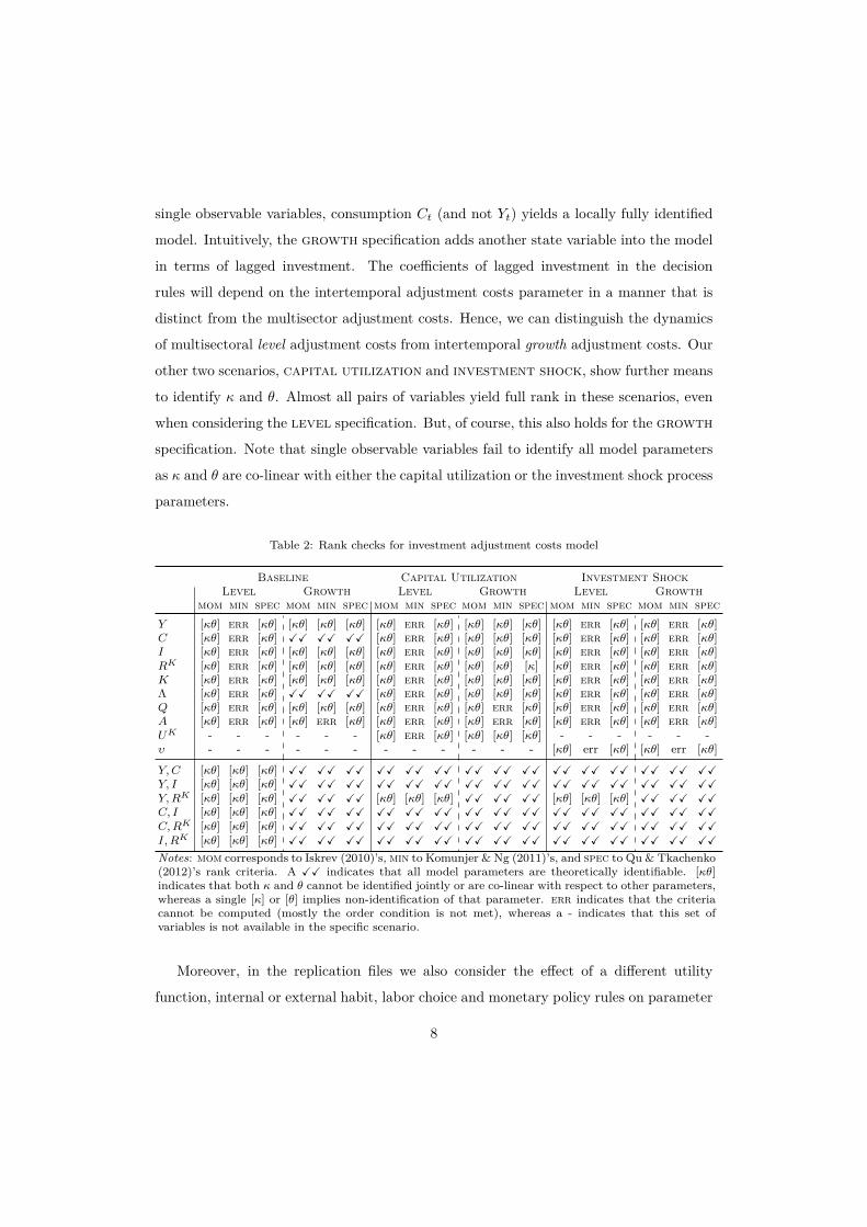
single observable variables, consumption Ct (and not Yt) yields a locally fully identified

model. Intuitively, the growth specification adds another state variable into the model

in terms of lagged investment. The coefficients of lagged investment in the decision

rules will depend on the intertemporal adjustment costs parameter in a manner that is

distinct from the multisector adjustment costs. Hence, we can distinguish the dynamics

of multisectoral level adjustment costs from intertemporal growth adjustment costs. Our

other two scenarios, capital utilization and investment shock, show further means

to identify κ and θ. Almost all pairs of variables yield full rank in these scenarios, even

when considering the level specification. But, of course, this also holds for the growth

specification. Note that single observable variables fail to identify all model parameters

as κ and θ are co-linear with either the capital utilization or the investment shock process

parameters.

Table 2: Rank checks for investment adjustment costs model

Baseline Capital Utilization Investment ShockLevel Growth Level Growth Level Growth

mom min spec mom min spec mom min spec mom min spec mom min spec mom min specY [κθ] err [κθ] [κθ] [κθ] [κθ] [κθ] err [κθ] [κθ] [κθ] [κθ] [κθ] err [κθ] [κθ] err [κθ]C [κθ] err [κθ] XX XX XX [κθ] err [κθ] [κθ] [κθ] [κθ] [κθ] err [κθ] [κθ] err [κθ]I [κθ] err [κθ] [κθ] [κθ] [κθ] [κθ] err [κθ] [κθ] [κθ] [κθ] [κθ] err [κθ] [κθ] err [κθ]RK [κθ] err [κθ] [κθ] [κθ] [κθ] [κθ] err [κθ] [κθ] [κθ] [κ] [κθ] err [κθ] [κθ] err [κθ]K [κθ] err [κθ] [κθ] [κθ] [κθ] [κθ] err [κθ] [κθ] [κθ] [κθ] [κθ] err [κθ] [κθ] err [κθ]Λ [κθ] err [κθ] XX XX XX [κθ] err [κθ] [κθ] [κθ] [κθ] [κθ] err [κθ] [κθ] err [κθ]Q [κθ] err [κθ] [κθ] [κθ] [κθ] [κθ] err [κθ] [κθ] err [κθ] [κθ] err [κθ] [κθ] err [κθ]A [κθ] err [κθ] [κθ] err [κθ] [κθ] err [κθ] [κθ] err [κθ] [κθ] err [κθ] [κθ] err [κθ]UK - - - - - - [κθ] err [κθ] [κθ] [κθ] [κθ] - - - - - -υ - - - - - - - - - - - - [κθ] err [κθ] [κθ] err [κθ]

Y,C [κθ] [κθ] [κθ] XX XX XX XX XX XX XX XX XX XX XX XX XX XX XXY, I [κθ] [κθ] [κθ] XX XX XX XX XX XX XX XX XX XX XX XX XX XX XXY,RK [κθ] [κθ] [κθ] XX XX XX [κθ] [κθ] [κθ] XX XX XX [κθ] [κθ] [κθ] XX XX XXC, I [κθ] [κθ] [κθ] XX XX XX XX XX XX XX XX XX XX XX XX XX XX XXC,RK [κθ] [κθ] [κθ] XX XX XX XX XX XX XX XX XX XX XX XX XX XX XXI, RK [κθ] [κθ] [κθ] XX XX XX XX XX XX XX XX XX XX XX XX XX XX XX

Notes: mom corresponds to Iskrev (2010)’s, min to Komunjer & Ng (2011)’s, and spec to Qu & Tkachenko(2012)’s rank criteria. A XX indicates that all model parameters are theoretically identifiable. [κθ]indicates that both κ and θ cannot be identified jointly or are co-linear with respect to other parameters,whereas a single [κ] or [θ] implies non-identification of that parameter. err indicates that the criteriacannot be computed (mostly the order condition is not met), whereas a - indicates that this set ofvariables is not available in the specific scenario.

Moreover, in the replication files we also consider the effect of a different utility

function, internal or external habit, labor choice and monetary policy rules on parameter

8

identification of θ and κ. We briefly summarize our findings. A CRRA utility function or

the inclusion of internal/external habit formation does not change the above results.5 The

inclusion of labor (as already shown by Kim (2003)) facilitates parameter identification of

θ and κ in both cases, but adds other parameters that can only be identified by observing

either hours or wages. Extending the baseline model with respect to bond holdings

requires the inclusion of a Taylor rule. This also provides means for identifying the

investment adjustment costs parameters in both the level and growth specification,

however, for several combinations of observables the parameters of the monetary rule are

not identified, a topic we study in more detail in the next section.

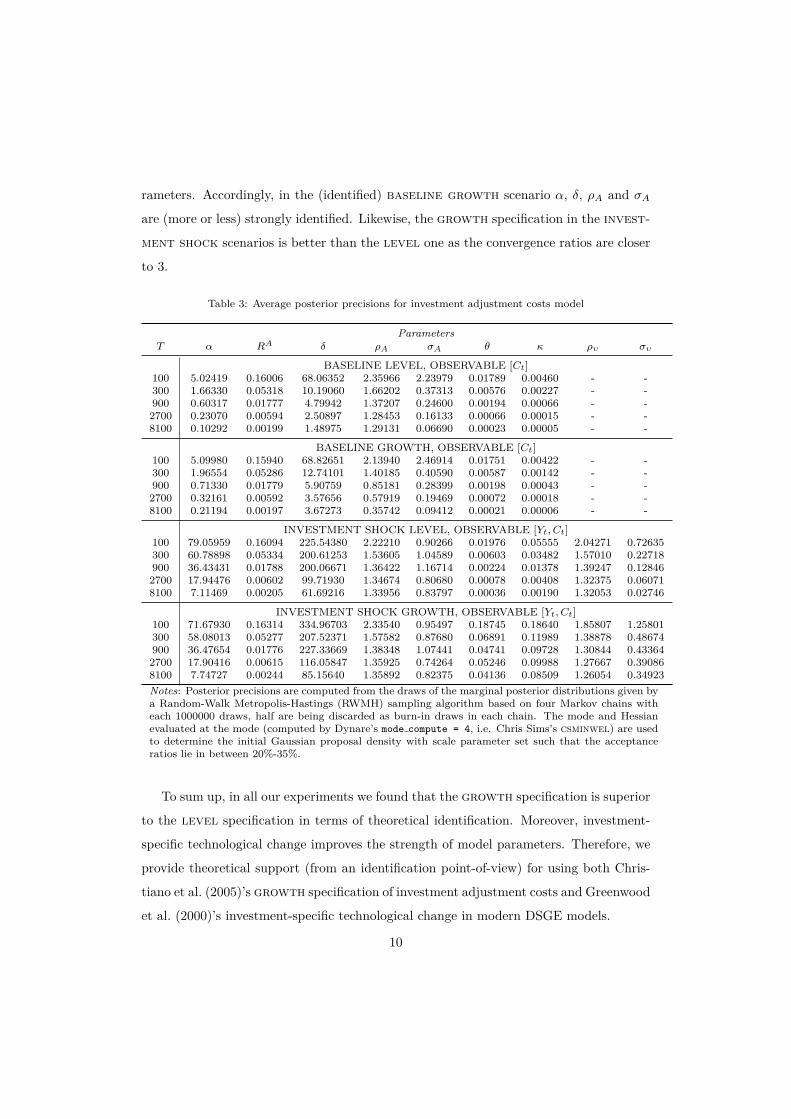
Tables 3 and 4 provide insight into the strength of identification according to the

Bayesian learning rate indicator of Koop et al. (2013) for the baseline scenario with

observable Ct and the investment shock scenario with observable Yt and Ct.6 The

simulation and estimation exercise reveals that the strength of identification of the in-

vestment adjustment costs parameters, θ and κ, is weak in both baseline scenarios as

well as the investment shock level case, since the rates at which the posterior pre-

cisions are updated are slower than the sample size change. In other words, the average

posterior precision values in the table tend towards zero instead of a constant value. This

is also evident by looking at the convergence ratios in table 4 as these stay close to 1 and

do not tend towards the change in samples size of 3. The investment shock growth

specification, however, is the exception, as κ and θ are both strongly identifiable: The

average precisions tend towards a constant and the convergence ratios fluctuate around

3. Regarding the other model parameters we find mixed results. In all cases under con-

sideration the strength of identification of RA (and hence β) is weak, which is a common

finding in the literature (Morris, 2017). In the (unidentified) baseline level scenario

we see that only ρA is strongly identifiable. This confirms that estimating non-identified

models yields severe problems in the estimation of other, actually identified model pa-

5In some cases we find that the identification criteria of Iskrev (2010), Komunjer & Ng (2011) andQu & Tkachenko (2012) yield different results. We experimented with the settings and found that thedifferences are driven by numerical thresholds, tolerance levels and the method used to normalize theJacobians for rank computations.

6We choose these scenarios due to the fact that our focus is on applied researchers who use Dynarefor Bayesian estimation. Accordingly, we do not analyze the strength of identification in the capitalutilization scenario as this requires techniques to estimate singular DSGE models, which cannot bedone with Dynare out-of-the-box (yet).

9

rameters. Accordingly, in the (identified) baseline growth scenario α, δ, ρA and σA

are (more or less) strongly identified. Likewise, the growth specification in the invest-

ment shock scenarios is better than the level one as the convergence ratios are closer

to 3.

Table 3: Average posterior precisions for investment adjustment costs model

ParametersT α RA δ ρA σA θ κ ρυ συ

BASELINE LEVEL, OBSERVABLE [Ct]100 5.02419 0.16006 68.06352 2.35966 2.23979 0.01789 0.00460 - -300 1.66330 0.05318 10.19060 1.66202 0.37313 0.00576 0.00227 - -900 0.60317 0.01777 4.79942 1.37207 0.24600 0.00194 0.00066 - -2700 0.23070 0.00594 2.50897 1.28453 0.16133 0.00066 0.00015 - -8100 0.10292 0.00199 1.48975 1.29131 0.06690 0.00023 0.00005 - -

BASELINE GROWTH, OBSERVABLE [Ct]100 5.09980 0.15940 68.82651 2.13940 2.46914 0.01751 0.00422 - -300 1.96554 0.05286 12.74101 1.40185 0.40590 0.00587 0.00142 - -900 0.71330 0.01779 5.90759 0.85181 0.28399 0.00198 0.00043 - -2700 0.32161 0.00592 3.57656 0.57919 0.19469 0.00072 0.00018 - -8100 0.21194 0.00197 3.67273 0.35742 0.09412 0.00021 0.00006 - -

INVESTMENT SHOCK LEVEL, OBSERVABLE [Yt, Ct]100 79.05959 0.16094 225.54380 2.22210 0.90266 0.01976 0.05555 2.04271 0.72635300 60.78898 0.05334 200.61253 1.53605 1.04589 0.00603 0.03482 1.57010 0.22718900 36.43431 0.01788 200.06671 1.36422 1.16714 0.00224 0.01378 1.39247 0.128462700 17.94476 0.00602 99.71930 1.34674 0.80680 0.00078 0.00408 1.32375 0.060718100 7.11469 0.00205 61.69216 1.33956 0.83797 0.00036 0.00190 1.32053 0.02746

INVESTMENT SHOCK GROWTH, OBSERVABLE [Yt, Ct]100 71.67930 0.16314 334.96703 2.33540 0.95497 0.18745 0.18640 1.85807 1.25801300 58.08013 0.05277 207.52371 1.57582 0.87680 0.06891 0.11989 1.38878 0.48674900 36.47654 0.01776 227.33669 1.38348 1.07441 0.04741 0.09728 1.30844 0.433642700 17.90416 0.00615 116.05847 1.35925 0.74264 0.05246 0.09988 1.27667 0.390868100 7.74727 0.00244 85.15640 1.35892 0.82375 0.04136 0.08509 1.26054 0.34923Notes: Posterior precisions are computed from the draws of the marginal posterior distributions given bya Random-Walk Metropolis-Hastings (RWMH) sampling algorithm based on four Markov chains witheach 1000000 draws, half are being discarded as burn-in draws in each chain. The mode and Hessianevaluated at the mode (computed by Dynare’s mode compute = 4, i.e. Chris Sims’s csminwel) are usedto determine the initial Gaussian proposal density with scale parameter set such that the acceptanceratios lie in between 20%-35%.

To sum up, in all our experiments we found that the growth specification is superior

to the level specification in terms of theoretical identification. Moreover, investment-

specific technological change improves the strength of model parameters. Therefore, we

provide theoretical support (from an identification point-of-view) for using both Chris-

tiano et al. (2005)’s growth specification of investment adjustment costs and Greenwood

et al. (2000)’s investment-specific technological change in modern DSGE models.

10

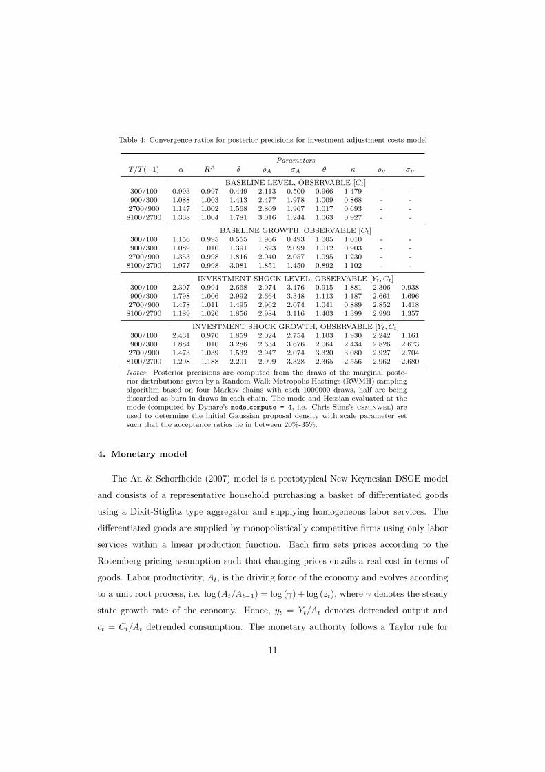
Table 4: Convergence ratios for posterior precisions for investment adjustment costs model

ParametersT/T (−1) α RA δ ρA σA θ κ ρυ συ

BASELINE LEVEL, OBSERVABLE [Ct]300/100 0.993 0.997 0.449 2.113 0.500 0.966 1.479 - -900/300 1.088 1.003 1.413 2.477 1.978 1.009 0.868 - -2700/900 1.147 1.002 1.568 2.809 1.967 1.017 0.693 - -8100/2700 1.338 1.004 1.781 3.016 1.244 1.063 0.927 - -

BASELINE GROWTH, OBSERVABLE [Ct]300/100 1.156 0.995 0.555 1.966 0.493 1.005 1.010 - -900/300 1.089 1.010 1.391 1.823 2.099 1.012 0.903 - -2700/900 1.353 0.998 1.816 2.040 2.057 1.095 1.230 - -8100/2700 1.977 0.998 3.081 1.851 1.450 0.892 1.102 - -

INVESTMENT SHOCK LEVEL, OBSERVABLE [Yt, Ct]300/100 2.307 0.994 2.668 2.074 3.476 0.915 1.881 2.306 0.938900/300 1.798 1.006 2.992 2.664 3.348 1.113 1.187 2.661 1.6962700/900 1.478 1.011 1.495 2.962 2.074 1.041 0.889 2.852 1.4188100/2700 1.189 1.020 1.856 2.984 3.116 1.403 1.399 2.993 1.357

INVESTMENT SHOCK GROWTH, OBSERVABLE [Yt, Ct]300/100 2.431 0.970 1.859 2.024 2.754 1.103 1.930 2.242 1.161900/300 1.884 1.010 3.286 2.634 3.676 2.064 2.434 2.826 2.6732700/900 1.473 1.039 1.532 2.947 2.074 3.320 3.080 2.927 2.7048100/2700 1.298 1.188 2.201 2.999 3.328 2.365 2.556 2.962 2.680Notes: Posterior precisions are computed from the draws of the marginal poste-rior distributions given by a Random-Walk Metropolis-Hastings (RWMH) samplingalgorithm based on four Markov chains with each 1000000 draws, half are beingdiscarded as burn-in draws in each chain. The mode and Hessian evaluated at themode (computed by Dynare’s mode compute = 4, i.e. Chris Sims’s csminwel) areused to determine the initial Gaussian proposal density with scale parameter setsuch that the acceptance ratios lie in between 20%-35%.

4. Monetary model

The An & Schorfheide (2007) model is a prototypical New Keynesian DSGE model

and consists of a representative household purchasing a basket of differentiated goods

using a Dixit-Stiglitz type aggregator and supplying homogeneous labor services. The

differentiated goods are supplied by monopolistically competitive firms using only labor

services within a linear production function. Each firm sets prices according to the

Rotemberg pricing assumption such that changing prices entails a real cost in terms of

goods. Labor productivity, At, is the driving force of the economy and evolves according

to a unit root process, i.e. log (At/At−1) = log (γ) + log (zt), where γ denotes the steady

state growth rate of the economy. Hence, yt = Yt/At denotes detrended output and

ct = Ct/At detrended consumption. The monetary authority follows a Taylor rule for

11

the nominal interest rate Rt and real government spending Gt is assumed to evolve

stochastically as a ratio of output gt := (1 − Gt/Yt)−1. Uncertainty is introduced via

random fluctuations in productivity growth, government spending and a monetary policy

shock.

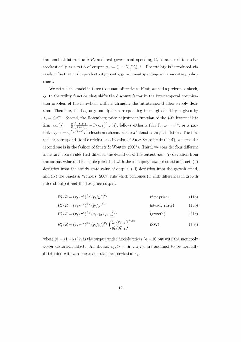
We extend the model in three (common) directions. First, we add a preference shock,

ζt, to the utility function that shifts the discount factor in the intertemporal optimiza-

tion problem of the household without changing the intratemporal labor supply deci-

sion. Therefore, the Lagrange multiplier corresponding to marginal utility is given by

λt = ζtc−τt . Second, the Rotemberg price adjustment function of the j-th intermediate

firm, act(j) = φ2

(Pt(j)Pt−1(j) − Γt,t−1

)2yt(j), follows either a full, Γt,t−1 = π∗, or a par-

tial, Γt,t−1 = πιp

t π∗1−ιp , indexation scheme, where π∗ denotes target inflation. The first

scheme corresponds to the original specification of An & Schorfheide (2007), whereas the

second one is in the fashion of Smets & Wouters (2007). Third, we consider four different

monetary policy rules that differ in the definition of the output gap: (i) deviation from

the output value under flexible prices but with the monopoly power distortion intact, (ii)

deviation from the steady state value of output, (iii) deviation from the growth trend,

and (iv) the Smets & Wouters (2007) rule which combines (i) with differences in growth

rates of output and the flex-price output.

R∗t /R = (πt/π∗)ψπ (yt/y∗

t )ψy (flex-price) (11a)

R∗t /R = (πt/π∗)ψπ (yt/y)ψy (steady state) (11b)

R∗t /R = (πt/π∗)ψπ (zt · yt/yt−1)ψy (growth) (11c)

R∗t /R = (πt/π∗)ψπ (yt/y∗

t )ψy(yt/yt−1

y∗t /y

∗t−1

)ψ∆y

(SW) (11d)

where y∗t = (1− ν) 1

τ gt is the output under flexible prices (φ = 0) but with the monopoly

power distortion intact. All shocks, εj,t(j = R, g, z, ζ), are assumed to be normally

distributed with zero mean and standard deviation σj .

12

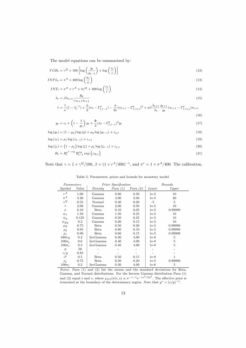
The model equations can be summarized by:

Y GRt = γQ + 100[log(

yt

yt−1

)+ log

(zt

z

)](12)

INFLt = πA + 400 log(πt

π

)(13)

INTt = πA + rA + 4γQ + 400 log(rt

r

)(14)

λt = βλt+1Rt

γzt+1πt+1(15)

1 =1ν

(1− λ−1t ) +

φ

2(πt − Γpt,t−1)−

φ

2ν(πt+1 − Γpt+1,t)

2 + φβλt+1

λt

yt+1

yt(πt+1 − Γpt+1,t)πt+1

(16)

yt = ct +(

1−1gt

)yt +

Φ2

(πt − Γpt,t−1)2yt (17)

log (gt) = (1− ρg) log (g) + ρg log (gt−1) + εg,t (18)

log (zt) = ρz log (zt−1) + εz,t (19)

log (ζt) =(1− ρζ

)log (ζ) + ρζ log (ζt−1) + εζ,t (20)

Rt = R∗1−ρRt R

ρRt−1 exp

{εR,t}

(21)

Note that γ = 1 + γQ/100, β = (1 + rA/400)−1, and π∗ = 1 + πA/400. The calibration,

Table 5: Parameters, priors and bounds for monetary model

Parameters Prior Specification BoundsSymbol Value Density Para (1) Para (2) Lower UpperrA 1.00 Gamma 0.80 0.50 1e-5 10πA 3.20 Gamma 4.00 2.00 1e-5 20γQ 0.55 Normal 0.40 0.20 -5 5τ 2.00 Gamma 2.00 0.50 1e-5 10ν 0.10 Beta 0.10 0.05 1e-5 0.99999ψπ 1.50 Gamma 1.50 0.25 1e-5 10ψy 0.125 Gamma 0.50 0.25 1e-5 10ψ∆y 0.2 Gamma 0.20 0.15 1e-5 10ρR 0.75 Beta 0.50 0.20 1e-5 0.99999ρg 0.95 Beta 0.80 0.10 1e-5 0.99999ρz 0.90 Beta 0.66 0.15 1e-5 0.99999

100σR 0.2 InvGamma 0.30 4.00 1e-8 5100σg 0.6 InvGamma 0.40 4.00 1e-8 5100σz 0.3 InvGamma 0.40 4.00 1e-8 5φ 50 - - - - -c/y 0.85 - - - - -ιp 0.5 Beta 0.50 0.15 1e-8 1ρζ 0.75 Beta 0.50 0.20 1e-5 0.99999

100σζ 0.2 InvGamma 0.30 4.00 1e-8 5Notes: Para (1) and (2) list the means and the standard deviations for Beta,Gamma, and Normal distributions. For the Inverse Gamma distribution Para (1)and (2) equal s and v, where ℘IG(σ|v, s) ∝ σ−v−1e−vs

2/2σ2 . The effective prior istruncated at the boundary of the determinacy region. Note that g∗ = (c/y)−1.

13

priors and bounds for the model parameters are given in table 5 and are taken from

An & Schorfheide (2007) and Smets & Wouters (2007). Note that Mutschler (2015)

shows that the set of parameters (ν, φ) and steady state ratio g∗ = yc do not enter the

linearized solution and are only identifiable via a higher-order approximation of the policy

functions. Therefore, we fix g∗ and φ throughout our analysis. The steady state is given

by normalizations, z = ζ = 1, π = π∗, g = g∗, and equations r = γzπβ , c = (1 − ν) 1

τ ,

y = g · c, Y GR = γQ, INFL = πA, INT = πA + rA + 4γQ.

In our sensitivity analysis of identifiability as a model property, we distinguish three

different model scenarios. Our first scenario, called baseline, corresponds to the original

model specification of An & Schorfheide (2007). Accordingly, we consider full inflation

indexation and switch off the discount factor shifter. In our second scenario, called

partial indexation, we analyze the effect of adding the partial inflation indexation

scheme to the baseline scenario. In our third scenario, called preference shock, we

add the discount factor shifter to the baseline model. We run all scenarios under the

four different monetary policy rules. We only discuss the results for observable variables

Y GRt, INFLt, and INTt here, as, apart from some steady state parameters like γQthat can only be identified from Y GR, other combinations of model variables do not

change our results significantly. We refer to the replication files for the full set of results,

i.e. for all possible combinations of up to three variables. Table 6 summarizes whether

the rank requirements are fulfilled for the different scenarios and monetary policy rules.

As shown by e.g. Komunjer & Ng (2011) or Qu & Tkachenko (2012), the monetary

policy parameters (ψy, ψπ, ρR, σR) cannot be identified in the baseline specification

when using the flex-price or the SW monetary rule, whereas in the steady state

or growth specification these parameters are locally identifiable. Our analysis shows

two more ways to dissolve the lack of identification, which are, moreover, independent of

the functional form of the Taylor rule: adding a preference shock and/or using a partial

inflation indexation scheme. Intuitively, this is due to their effect on the transmission

channel of monetary policy as noted by e.g. Schmitt-Grohe & Uribe (2004a).

Tables 7 and 8 give insight into the strength of identification according to the Bayesian

learning rate indicator of Koop et al. (2013) for the flex-price baseline, steady state

baseline, flex-price preference shock and flex-price indexation scenarios. We

14

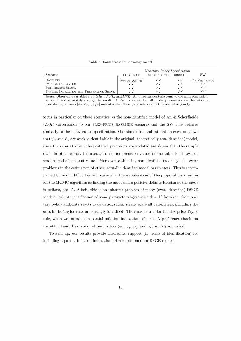
Table 6: Rank checks for monetary model

Monetary Policy SpecificationScenario flex-price steady state growth SWBaseline [ψπ , ψy , ρR, σR] XX XX [ψπ , ψy , ρR, σR]Partial Indexation XX XX XX XXPreference Shock XX XX XX XXPartial Indexation and Preference Shock XX XX XX XX

Notes: Observable variables are Y GRt, INFLt and INTt. All three rank criteria come to the same conclusion,so we do not separately display the result. A XX indicates that all model parameters are theoreticallyidentifiable, whereas [ψπ , ψy , ρR, ρσ ] indicates that these parameters cannot be identified jointly.

focus in particular on these scenarios as the non-identified model of An & Schorfheide

(2007) corresponds to our flex-price baseline scenario and the SW rule behaves

similarly to the flex-price specification. Our simulation and estimation exercise shows

that ψπ and ψy are weakly identifiable in the original (theoretically non-identified) model,

since the rates at which the posterior precisions are updated are slower than the sample

size. In other words, the average posterior precision values in the table tend towards

zero instead of constant values. Moreover, estimating non-identified models yields severe

problems in the estimation of other, actually identified model parameters. This is accom-

panied by many difficulties and caveats in the initialization of the proposal distribution

for the MCMC algorithm as finding the mode and a positive definite Hessian at the mode

is tedious, see A. Albeit, this is an inherent problem of many (even identified) DSGE

models, lack of identification of some parameters aggravates this. If, however, the mone-

tary policy authority reacts to deviations from steady state all parameters, including the

ones in the Taylor rule, are strongly identified. The same is true for the flex-price Taylor

rule, when we introduce a partial inflation indexation scheme. A preference shock, on

the other hand, leaves several parameters (ψπ, ψy, ρζ , and σζ) weakly identified.

To sum up, our results provide theoretical support (in terms of identification) for

including a partial inflation indexation scheme into modern DSGE models.

15

Table 7: Average posterior precisions for monetary model

PARAMETERST rA πA γQ τ ν ψπ ψy ρR ρg ρz 100σR 100σg 100σz ρζ 100σζ ιp

BASELINE WITH FLEX-PRICE TAYLOR RULE (*)100 0.061 0.270 0.461 0.068 38.082 0.228 2.818 5.493 3.363 29.575 40.687 3.981 11.028 - - -300 0.034 0.146 0.228 0.049 32.200 0.075 1.141 4.722 8.228 19.407 36.607 5.294 10.092 - - -900 0.020 0.085 0.155 0.034 24.358 0.031 0.722 4.746 9.009 19.107 43.514 5.551 11.034 - - -2700 0.018 0.075 0.131 0.036 25.799 0.010 0.262 4.821 8.305 20.746 45.198 5.535 14.533 - - -8100 0.016 0.068 0.121 0.037 27.490 0.004 0.108 4.449 8.183 21.107 43.708 5.567 15.825 - - -

BASELINE WITH STEADY STATE TAYLOR RULE100 0.055 0.145 0.444 0.055 40.977 0.279 2.779 4.398 3.865 34.385 40.505 3.206 9.897 - - -300 0.030 0.049 0.226 0.050 31.939 0.101 0.853 3.678 17.043 14.894 35.231 3.558 5.383 - - -900 0.017 0.046 0.145 0.024 18.887 0.075 1.748 4.164 17.572 17.036 43.902 4.465 5.656 - - -2700 0.016 0.045 0.122 0.022 16.903 0.054 1.471 4.197 14.471 17.612 45.664 4.491 5.992 - - -8100 0.015 0.043 0.125 0.021 17.104 0.058 1.778 3.940 13.030 16.057 43.692 4.628 6.020 - - -

PREFERENCE SHOCK WITH FLEX-PRICE TAYLOR RULE (*)100 0.063 0.268 0.481 0.087 61.319 0.221 2.025 4.037 2.278 20.611 32.155 1.751 10.793 0.276 0.339 -300 0.034 0.157 0.241 0.040 32.052 0.077 1.067 4.426 4.122 19.996 35.010 3.069 9.786 0.086 0.241 -900 0.022 0.092 0.151 0.038 27.964 0.028 0.615 4.716 4.468 20.622 39.890 1.802 10.865 0.031 0.094 -2700 0.023 0.086 0.153 0.034 22.883 0.010 0.271 4.080 7.164 18.756 41.170 1.228 11.017 0.013 0.055 -8100 0.017 0.070 0.117 0.036 26.957 0.003 0.084 4.599 8.017 21.936 42.120 1.331 14.445 0.005 0.030 -

INDEXATION WITH FLEX-PRICE TAYLOR RULE (*)100 0.061 0.114 0.451 0.065 47.761 0.280 0.991 7.112 3.136 20.011 38.531 4.058 4.586 - - 2.998300 0.035 0.064 0.232 0.050 41.508 0.110 0.443 5.540 7.330 16.998 33.627 5.341 5.440 - - 2.599900 0.020 0.035 0.148 0.029 26.825 0.063 0.341 5.555 8.928 18.567 40.908 5.454 4.947 - - 2.5332700 0.018 0.030 0.122 0.033 27.352 0.027 0.182 5.442 8.287 21.504 40.337 5.572 6.773 - - 2.6138100 0.018 0.032 0.129 0.033 28.766 0.023 0.154 5.070 8.175 22.077 39.142 5.596 6.651 - - 2.458Notes: Observable variables are Y GRt, INFLt, and INTt. Posterior precisions are computed from the draws of the marginal posterior distributionsgiven by a Random-Walk Metropolis-Hastings (RWMH) sampling algorithm based on four Markov chains with each 1000000 draws, half are beingdiscarded as burn-in draws in each chain. The mode and Hessian evaluated at the mode (computed by Dynare’s mode compute=4, i.e. Chris Sims’scsminwel) are used to determine the initial Gaussian proposal density with scale parameter set such that the acceptance ratios lie in between 20%-35%.A (*) indicates cases where we used an advanced mode finding procedure, as outlined in A.

16

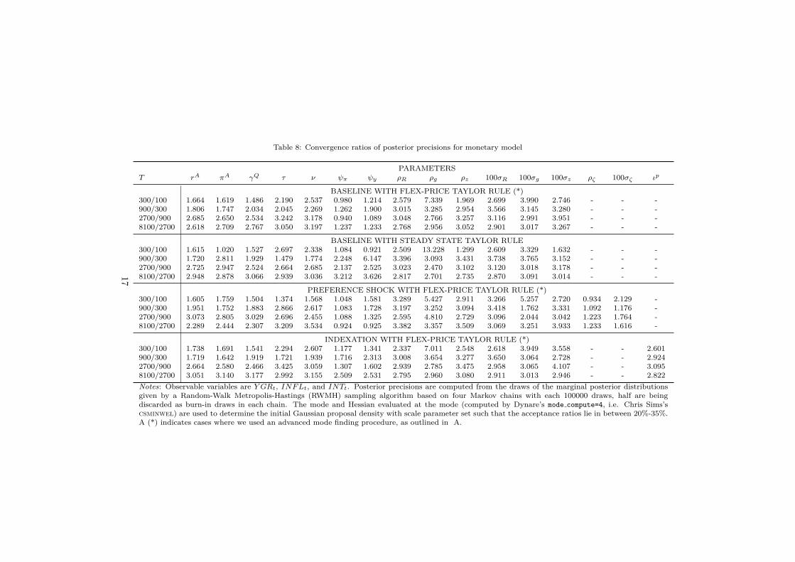
Table 8: Convergence ratios of posterior precisions for monetary model

PARAMETERST rA πA γQ τ ν ψπ ψy ρR ρg ρz 100σR 100σg 100σz ρζ 100σζ ιp

BASELINE WITH FLEX-PRICE TAYLOR RULE (*)300/100 1.664 1.619 1.486 2.190 2.537 0.980 1.214 2.579 7.339 1.969 2.699 3.990 2.746 - - -900/300 1.806 1.747 2.034 2.045 2.269 1.262 1.900 3.015 3.285 2.954 3.566 3.145 3.280 - - -2700/900 2.685 2.650 2.534 3.242 3.178 0.940 1.089 3.048 2.766 3.257 3.116 2.991 3.951 - - -8100/2700 2.618 2.709 2.767 3.050 3.197 1.237 1.233 2.768 2.956 3.052 2.901 3.017 3.267 - - -

BASELINE WITH STEADY STATE TAYLOR RULE300/100 1.615 1.020 1.527 2.697 2.338 1.084 0.921 2.509 13.228 1.299 2.609 3.329 1.632 - - -900/300 1.720 2.811 1.929 1.479 1.774 2.248 6.147 3.396 3.093 3.431 3.738 3.765 3.152 - - -2700/900 2.725 2.947 2.524 2.664 2.685 2.137 2.525 3.023 2.470 3.102 3.120 3.018 3.178 - - -8100/2700 2.948 2.878 3.066 2.939 3.036 3.212 3.626 2.817 2.701 2.735 2.870 3.091 3.014 - - -

PREFERENCE SHOCK WITH FLEX-PRICE TAYLOR RULE (*)300/100 1.605 1.759 1.504 1.374 1.568 1.048 1.581 3.289 5.427 2.911 3.266 5.257 2.720 0.934 2.129 -900/300 1.951 1.752 1.883 2.866 2.617 1.083 1.728 3.197 3.252 3.094 3.418 1.762 3.331 1.092 1.176 -2700/900 3.073 2.805 3.029 2.696 2.455 1.088 1.325 2.595 4.810 2.729 3.096 2.044 3.042 1.223 1.764 -8100/2700 2.289 2.444 2.307 3.209 3.534 0.924 0.925 3.382 3.357 3.509 3.069 3.251 3.933 1.233 1.616 -

INDEXATION WITH FLEX-PRICE TAYLOR RULE (*)300/100 1.738 1.691 1.541 2.294 2.607 1.177 1.341 2.337 7.011 2.548 2.618 3.949 3.558 - - 2.601900/300 1.719 1.642 1.919 1.721 1.939 1.716 2.313 3.008 3.654 3.277 3.650 3.064 2.728 - - 2.9242700/900 2.664 2.580 2.466 3.425 3.059 1.307 1.602 2.939 2.785 3.475 2.958 3.065 4.107 - - 3.0958100/2700 3.051 3.140 3.177 2.992 3.155 2.509 2.531 2.795 2.960 3.080 2.911 3.013 2.946 - - 2.822Notes: Observable variables are Y GRt, INFLt, and INTt. Posterior precisions are computed from the draws of the marginal posterior distributionsgiven by a Random-Walk Metropolis-Hastings (RWMH) sampling algorithm based on four Markov chains with each 100000 draws, half are beingdiscarded as burn-in draws in each chain. The mode and Hessian evaluated at the mode (computed by Dynare’s mode compute=4, i.e. Chris Sims’scsminwel) are used to determine the initial Gaussian proposal density with scale parameter set such that the acceptance ratios lie in between 20%-35%.A (*) indicates cases where we used an advanced mode finding procedure, as outlined in A.

17

5. Discussion of results

First, both theoretical lack of and empirical weak identification are often due to an

unfortunate choice of observables. In some cases, like the steady state parameters in our

monetary model, this seems obvious. In other cases, like in our investment-adjustment

costs model, one should use a specific observable variable (e.g. consumption) instead of

other, commonly used ones (e.g. output). In this line of thought, Kim (2003) already

pointed out, that information on the relative price of investment can also solve the

identification problem, and hence, it is not surprising that current papers include this

price in estimated DSGE models, see e.g. Justiniano et al. (2011). As the literature

on the choice of observables is still very sparse (Canova et al., 2014; Guerron-Quintana,

2010), we advocate (and show means) to do a brute-force sensitivity analysis before taking

a model to actual data. Second, our results show that the identification failure in the

Kim (2003) model can be dissolved by specifying intertemporal investment adjustment

costs in terms of growth instead of the investment-capital ratio, whereas specifying the

output-gap in terms of deviations from steady state or trend-growth identifies the An

& Schorfheide (2007) model. Third, by using model features like capital utilization in

the first model or partial inflation indexation in the second model, one can identify the

models independent of the concrete specification of investment adjustment costs or Taylor

rule. Fourth, the same is true when adding an investment-specific technological shock in

the former or a preference shock in the latter model.

Our results are relevant from a model building perspective, because it is crucial for

macroeconomists to know what frictions and shocks can coexist within models without

redundancy. Hence, on the one hand, our finding that the investment-growth specification

of intertemporal costs is not subject to functional equivalence with multisectoral costs is

useful, especially since this specification is now the benchmark in the quantitative DSGE

literature. Accordingly, a recent example is Moura (2018) who is able to use both types

of costs to study investment price rigidities in a multisectoral DSGE model. On the other

hand, our findings show that by adding different model features and/or shocks one is even

able to identify models with both multisectoral and intertemporal level costs. Our results

are not limited to investment. Similar specifications are used to model imperfect labor

mobility between the consumption-sector and the investment-sector, see e.g. (Nadeau,18

2009, Ch.2). Likewise, the monetary policy rule needs to be specified carefully. But our

findings show that including a partial inflation indexation scheme provides researchers

with more flexibility in the precise shape of the Taylor rule.

6. Conclusion

We strongly recommend that researchers should treat parameter identification as a

model property, i.e. from a model building perspective. A wise choice on observables or

slight and subtle changes in model assumptions, functional specifications, or structural

shocks have an impact on both theoretical (yes/no) identification properties as well as

on the strength of identification. In this regard, we side with Adolfson et al. (2019)

who argue that “lack of identification should neither be ignored nor be assumed to affect

all DSGE models, [. . . ] identification problems can be readily assessed on a case-by-case

basis”. We extend their approach by using different diagnostic tools for theoretical as well

as empirical identification properties and also show means to dissolve the identification

failures. Moreover, our paper also has a computational contribution as our research feeds

into and extends Dynare’s (Adjemian et al., 2011) identification toolbox. In particular,

we provide means to analyze the criteria of Komunjer & Ng (2011) and Qu & Tkachenko

(2012) by using analytical (instead of numerical) derivatives to compute the relevant

Jacobians. Lastly, as our example models are of small scale and easy to replicate and

extend, they should be useful for both applied and theoretical macroeconomists as well

as for teaching purposes.

19

References

Adjemian, S., Bastani, H., Juillard, M., Karame, F., Maih, J., Mihoubi, F., Perendia, G., Pfeifer, J.,

Ratto, M., & Villemot, S. (2011). Dynare: Reference Manual Version 4 . Dynare Working Papers 1

CEPREMAP.

Adolfson, M., Laseen, S., Linde, J., & Ratto, M. (2019). Identification versus misspecification in

New Keynesian monetary policy models. European Economic Review, 113 , 225–246. doi:10.1016/j.

euroecorev.2018.12.010.

An, S., & Schorfheide, F. (2007). Bayesian Analysis of DSGE Models. Econometric Reviews, 26 ,

113–172. doi:10.1080/07474930701220071.

Andreasen, M. M. (2010). How to Maximize the Likelihood Function for a DSGE Model. Computational

Economics, 35 , 127–154. doi:10.1007/s10614-009-9182-6.

Canova, F., Ferroni, F., & Matthes, C. (2014). Choosing the variables to estimate singular DSGE models.

Journal of Applied Econometrics, 29 , 1099–1117. doi:10.1002/jae.2414.

Canova, F., & Sala, L. (2009). Back to square one: Identification issues in DSGE models. Journal of

Monetary Economics, 56 , 431–449. doi:10.1016/j.jmoneco.2009.03.014.

Chadha, J., & Shibayama, K. (2018). Bayesian Estimation of DSGE models: Identification using a

diagnostic indicator . Working Paper NIESR and University of Kent.

Christiano, L. J., Eichenbaum, M., & Evans, C. L. (2005). Nominal Rigidities and the Dynamic Effects

of a Shock to Monetary Policy. Journal of Political Economy, 113 , 1–45. doi:10.1086/426038.

Fernandez-Villaverde, J., Rubio-Ramırez, J. F., & Schorfheide, F. (2016). Solution and Estimation

Methods for DSGE Models. In J. B. Taylor, & H. Uhlig (Eds.), Handbook of Macroeconomics (pp.

527–724). North-Holland volume 2. doi:10.1016/bs.hesmac.2016.03.006.

Greenwood, J., Hercowitz, Z., & Krusell, P. (2000). The role of investment-specific technological change

in the business cycle. European Economic Review, 44 , 91–115. doi:10.1016/S0014-2921(98)00058-0.

Guerron-Quintana, P. A. (2010). What you match does matter: the effects of data on DSGE estimation.

Journal of Applied Econometrics, 25 , 774–804. doi:10.1002/jae.1106.

Huffman, G. W., & Wynne, M. A. (1999). The role of intratemporal adjustment costs in a multisector

economy. Journal of Monetary Economics, 43 , 317–350. doi:10.1016/S0304-3932(98)00059-2.

Iskrev, N. (2010). Local identification in DSGE models. Journal of Monetary Economics, 57 , 189–202.

doi:10.1016/j.jmoneco.2009.12.007.

Justiniano, A., Primiceri, G. E., & Tambalotti, A. (2010). Investment shocks and business cycles. Journal

of Monetary Economics, 57 , 132–145. doi:10.1016/j.jmoneco.2009.12.008.

Justiniano, A., Primiceri, G. E., & Tambalotti, A. (2011). Investment shocks and the relative price of

investment. Review of Economic Dynamics, 14 , 102–121. doi:10.1016/j.red.2010.08.004.

Kamber, G., McDonald, C., Sander, N., & Theodoridis, K. (2016). Modelling the business cycle of a

small open economy: The Reserve Bank of New Zealand’s DSGE model. Economic Modelling, 59 ,

546–569. doi:10.1016/j.econmod.2016.08.013.

Kim, J. (2003). Functional Equivalence between Intertemporal and Multisectoral Investment Adjust-

20

ment Costs. Journal of Economic Dynamics and Control, 27 , 533–549. doi:10.1016/s0165-1889(01)

00060-4.

Komunjer, I., & Ng, S. (2011). Dynamic Identification of Dynamic Stochastic General Equilibrium

Models. Econometrica, 79 , 1995–2032. doi:10.3982/ECTA8916.

Koop, G., Pesaran, M. H., & Smith, R. P. (2013). On Identification of Bayesian DSGE Models. Journal

of Business & Economic Statistics, 31 , 300–314. doi:10.1080/07350015.2013.773905.

Lucas, R. E., & Prescott, E. C. (1971). Investment under Uncertainty. Econometrica, 39 , 659–681.

doi:10.2307/1909571.

Morris, S. D. (2017). DSGE pileups. Journal of Economic Dynamics and Control, 74 , 56–86. doi:10.

1016/j.jedc.2016.11.002.

Moura, A. (2018). Investment shocks, sticky prices, and the endogenous relative price of investment.

Review of Economic Dynamics, 27 , 48–63. doi:10.1016/j.red.2017.11.004.

Mutschler, W. (2015). Identification of DSGE models – The effect of higher-order approximation and

pruning. Journal of Economic Dynamics and Control, 56 , 34–54. doi:10.1016/j.jedc.2015.04.007.

Mutschler, W. (2016). Local identification of nonlinear and non-Gaussian DSGE models. Number 10

in Wissenschaftliche Schriften der WWU Munster, Reihe IV. Munster: Monsenstein und Vannerdat.

PhD Thesis.

Mutschler, W. (2019). Improvement of Identification Toolbox (Merge Request). https://git.dynare.

org/Dynare/dynare/merge_requests/1648. [Online; accessed May-7-2019].

Nadeau, J.-F. (2009). Essays in Macroeconomics. PhD Thesis University of Britisch Columbia Vancou-

ver.

Qu, Z., & Tkachenko, D. (2012). Identification and frequency domain quasi-maximum likelihood estima-

tion of linearized dynamic stochastic general equilibrium models. Quantitative Economics, 3 , 95–132.

doi:10.3982/QE126.

Ratto, M., & Iskrev, N. I. (2011). Identification analysis of DSGE models with DYNARE. MONFISPOL

225149 European Commission and Banco de Portugal.

Rıos-Rull, J.-V., Schorfheide, F., Fuentes-Albero, C., Kryshko, M., & Santaeulalia-Llopis, R. (2012).

Methods versus substance: Measuring the effects of technology shocks. Journal of Monetary Eco-

nomics, 59 , 826–846. doi:10.1016/j.jmoneco.2012.10.008.

Schmitt-Grohe, S., & Uribe, M. (2004a). Optimal fiscal and monetary policy under sticky prices. Journal

of Economic Theory, 114 , 198–230. doi:10.1016/S0022-0531(03)00111-X.

Schmitt-Grohe, S., & Uribe, M. (2004b). Optimal Operational Monetary Policy in the Christiano-

Eichenbaum-Evans Model of the U.S. Business Cycle. Working Paper 10724 National Bureau of

Economic Research. doi:10.3386/w10724.

Smets, F., & Wouters, R. (2007). Shocks and Frictions in US Business Cycles: A Bayesian DSGE

Approach. American Economic Review, 97 , 586–606. doi:10.1257/aer.97.3.586.

21

A. Posterior mode finding

We use an advanced mode finding procedure, where we sequentially loop over different

optimization algorithms taking the previous found mode as initial value for the next

optimizer. In particular, we loop, in this order, over Dynare’s mode compute values

equal to 9 (CMA-ES), 8 (Nelson-Mead Simplex), 4 (csminwel), 7 (fminsearch) and 1

(fmincon). We then rely on Dynare’s (very time-consuming) mode compute=6 optimizer,

i.e. a “Monte Carlo Optimizer” to get a well-behaved Hessian in the relevant parameter

space. The intuition is that the Metropolis-Hastings algorithm does not need to start

from the posterior mode to converge to the posterior distribution. It is only required

to start from a point with a high posterior density value and to use an estimate of the

covariance matrix for the jumping distribution (actually any positive definite matrix will

suffice). As a side note, the replication files of An & Schorfheide (2007) reveal that they

face the same problem in their estimation and overcome this by using different step sizes

for the numerical evaluation of second derivatives of the log-likelihood function.

22