the effect of local area crime on mental healthuctpb21/cpapers/areacrimeandmentalhealth.pdfthe...

THE EFFECT OF LOCAL AREA CRIME ON MENTALHEALTH*

Christian Dustmann and Francesco Fasani

This study analyses the effect of local crime rates on residents’ mental health. Using longitudinalinformation on individuals’ mental well-being, we address the problem of sorting and endogenousmoving behaviour. We find that crime causes considerable mental distress for residents, primarilydriven by property crime. Effects are stronger for females, and mainly related to depression andanxiety. The distress caused by one SD increase in local crime is 2–4 times larger than that caused bya 1 SD decrease in local employment, and about one-seventh of the short-term impact of the 7 July2005 London Bombings.

According to the Eurobarometer, crime has been among the top five concerns ofEuropean citizens in recent years and the fight against crime is among the mainpriorities respondents believe their governments should have.1 These concerns seemhardly justified by actual crime rates, where European countries rank very low incomparison to other parts of the world,2 which suggests that crime leads to distressfor a large part of the population through channels other than direct victimisation.These indirect costs of crime, through inflicting fear and anxiety, and leading tochanges in daily routines and behaviour (Hamermesh, 1999; Braakman, 2013; Jankeet al., 2013), may be far larger than the direct costs. Indeed, in a recent paper,Becker and Rubinstein (2011) argue that major criminal acts such as terroristattacks inflict most harm by creating fear and by inducing changes in behaviourand individual choices. Measuring the magnitude of these indirect costs of crime iscrucial for assessing the optimal investment into crime prevention. While the directcosts (response costs of police and the Criminal Justice System, and costs through

* Corresponding author: F. Fasani, Department of Economics and Finance, Queen Mary University ofLondon, 327 Mile End Road, E1 4NS, London, UK. Email: [email protected].

We are grateful to David Card, Francesca Cornaglia, Thomas Cornelissen, Guglielmo Weber, aneditor and two anonymous referees for comments and suggestions. We would like to thankparticipants in conferences, workshops and seminars at IAE-CSIC (Barcelona), University of MilanBicocca, Collegio Carlo Alberto (Turin), University of Alicante and EUI (Fiesole). We acknowledgefinancial support from the UK Economic and Social Research Council (‘Crime and mental wellbeing’;grant number: RES-000-22-1979). Fasani acknowledges the financial support of INSIDE-MOVE (Markets,Organizations and Votes in Economics), the Barcelona GSE Research Network, the Government ofCatalonia (grant 2009 SGR 896), the JAE-Doc grant for the programme ‘Junta para la Ampliaci�on deEstudios’ co-financed by the European Social Fund and the Spanish Ministry of Science (grant ECO2011-25293). Dustmann acknowledges funding by the Norface programme on migration. The usual disclaimerapplies.

1 Summary reports on Eurobarometer waves since 1974 can be downloaded at: http://ec.europa.eu/public_opinion/archives/eb_arch_en.htm.

2 For instance, over the last decade, EU27 countries experienced a homicide rate below 2per 100 thousand population, which contrasts with a world estimate of almost 8 (estimated in 2004)and with average rates in Southern Africa and Central America between 20 and 30 (Harrendorf et al.,2010).

[ 1 ]

The Economic Journal,Doi: 10.1111/ecoj.12205© 2014Royal Economic Society. Published by John Wiley & Sons, 9600 Garsington Road, Oxford OX4

2DQ, UK and 350 Main Street, Malden, MA 02148, USA.

the impact on victims) are routinely assessed,3 evaluations of indirect costs,including those of non-victims, are scarce, and far more difficult.

In this study, we analyse costs of crime that are indirect and intangible. Whileindirect but tangible costs – such as changes in behaviour (not going out at night, notwearing jewellery, carrying a self-defence weapon etc.) and investment in security(burglar alarms, armoured doors and windows, weapons etc.) – can in principle beinferred from surveys, intangible costs (fear, anxiety, mental distress etc.) areparticularly difficult to measure. Our main contribution is to estimate the effect localcrime has on the mental health of individuals who live in the area where this crimetakes place, by combining official crime statistics with detailed information onindividuals’ mental well-being, which we obtain from the British Household PanelSurvey (BHPS) and the English Longitudinal Study of Ageing (ELSA). Both thesesurveys are panel surveys, which allows us to use a design that eliminates possiblecorrelation between area crime and mental distress due to sorting of more distressedindividuals into areas with higher (or lower) crime incidences. By matching eachindividual to detailed local-area crime statistics for various types of crimes, we are ableto distinguish further between the effects that particular types of crime have on mentalhealth, thus identifying the most distressing criminal offences. We also analyse theimpact of crime on different dimensions of mental health and we study heterogeneityin responses across different groups of residents.

Our findings show a significant, and negative, impact of overall local crime rates onthe mental distress of residents in urban areas. The impact is sizeable: a 1 SD increasein the overall local crime rate causes an increase in mental distress that accounts forbetween 8% and 15% of the (within-individual) standard deviation in self-reportedmental well-being. This is about twice to four times as large as the effect of a 1 SDdecrease in the areas’ employment rate on mental distress. Burglary, car theft andvandalism are the crime types which seem to cause major anguish. In addition, we findheterogeneity in responses. While individuals react only to property crime when crimerates are measured in the immediate residential location, violent crime causes mentaldistress when including the surrounding areas, suggesting that this crime type impactsthrough affecting individuals’ daily routines, like travel to work etc. When distinguish-ing between men and women, we find that women are more responsive to changes incrime rates than men. Our results based on the ELSA, a data set which containsalternative measures of mental health and focuses on a particularly vulnerable group,those above the age of 50, produces very similar results.

To assess the magnitude of our findings further, we estimate the effect of theLondon bombings on the 7 July 2005 on mental distress. Using a difference-in-differences approach, we show that in the months following the attack, citizens ofLondon and the other major cities in the UK experienced a significant drop in their

3 See Soares (2010) for a recent survey of the different approaches to estimating costs of crime. In its mostrecent estimation, the UK Home Office puts the cost of crime against individuals and households in the UKat about £36.2 bn in 2003/04, which amounts to about 3% of GDP (Dubourg et al., 2005). Following themethodology suggested in Dolan et al. (2005), these estimates carefully appraise ‘physical and emotionalimpact on direct victims’ – which accounts for about 50% of total cost of crime. However, they do notconsider the additional cost imposed by the fear of crime on the overall British society, which is one objectiveof this study.

© 2014 Royal Economic Society.

2 T H E E CONOM I C J O U RN A L

self-reported mental health. We find that the reduction in mental wellbeing following a1 SD increase in local crime is about one-seventh of the fall in mental well-being causedby the London Bombings.

Our article contributes to the literature on estimating intangible costs of crime byfocusing on a new and specific aspect. While most of the previous literature hasimplemented either contingent valuation methods based on stated preferences(Cohen et al., 2004; Atkinson et al., 2005),4 or hedonic price models based onrevealed preferences (Gibbons, 2004; Linden and Rockoff, 2008),5 our study focuseson the detrimental impact of exposure to changes in local crime on mental well-beingof residents. Our work is also related to a recent paper by Cornaglia et al. (2014) on therelationship between mental well-being and crime for Australia.6 While Cornaglia et al.(2014) focus most of their discussion on the difference between being victimised andbeing exposed to crime (but not victimised), our article develops an in-depth analysisof the consequences for mental health of exposure to local crime.7

Our article is also related to the literature on neighbourhood effects and mentalwell-being. Several non-experimental studies – almost entirely based on cross-sectionalanalysis – find significant associations between the mental health of residents andaspects of the neighbourhood environment.8 Based on the Moving to Opportunity(MTO) experiment, a randomised experiment on residential mobility conducted infive US cities in the 1990s, a number of studies have shown that moving away fromdeprived (high crime) neighbourhoods leads to significant improvements in adultphysical and mental health and subjective well-being in the short (Katz et al., 2001),medium (Kling et al., 2007) and long term (Ludwig et al., 2012).9 We add to thisliterature by focusing on the direct link between area crime rates and mental distress ofresidents who are living in the area, and by providing a precise assessment of themagnitude of these effects. We use longitudinal data and exploit repeated informationon both mental well-being and area crime to eliminate potential sorting biases.Moreover, we analyse which specific dimensions of mental well-being are affected bycrime, we distinguish the effects of different types of crime on mental distress and weassess the heterogeneity in responses across different population groups.

4 See Hausman (2012) for a criticism of the reliability of contingent valuation methods in assessing socialcosts of changes in environmental quality, and a more positive assessment by Carson (2012).

5 Gibbons (2004) and Linden and Rockoff (2008) show that house prices fall in response to, respectively,increases in local property crime and the presence of convicted sexual offenders in the area. Similarly, Besleyand Mueller (2012) look at the impact of conflict in Northern Ireland (rather than crime) and establish anegative correlation between killings and house prices.

6 The two papers were part of the project ‘Crime and mental wellbeing’ supported by an ESRC grant(grant number: RES-000-22-1979).

7 With respect to Cornaglia et al. (2014), we use two alternative data sets, three different measures ofmental health and measures of crime rates at two levels of geographical disaggregation. Further, we analyseboth timing and heterogeneity of the effects, consider single mental health items and single criminaloffences and benchmark the magnitude of the effects we find against the mental health consequences of amajor terrorist attack.

8 See Mair et al. (2008) and Diez-Roux and Mair (2010) for recent reviews of this literature. In the UK,Propper et al. (2005) find a limited association between neighbourhood characteristics and levels (andchanges) in mental health of residents.

9 Oreopoulos (2003) exploits quasi-experimental variation in assignment to different public housingprojects in Toronto to estimate the impact of neighbourhood characteristics on long-term labour marketoutcomes of residents but does not investigate health and mental well-being as possible outcomes.


E F F E C T O F L O C A L A R E A C R I M E ON M EN T A L H E A L TH 3

The research we provide in this article adds to the policy debate on the cost ofmental distress to the overall society and on the role played by crime in reducingpeople’s well-being. Layard (2005) argues that mental issues represent one of thebiggest problems in British society, with serious consequences for the welfare system.He estimates the cost of mental illness at about 2% of GDP.10 Crime is an importantaggravating factor: According to the National Institute for Mental Health in England(2005), reducing fear of crime would improve mental health and well-being of Britain’spopulations. Following an influential independent report on health inequalitiesproduced in the late 1990s (Acheson, 1998), the British Department of Healthidentified decreasing exposure to crime in the neighbourhood as a crucial policy torestrict disparities in health hazard among the British population (Department ofHealth, 1999) and this is still a key focus of their intervention (Department of Health,2009). Clearly, the problem is not limited to Britain. The WHO Commission on SocialDeterminants of Health recognised the level of crime and violence in the area ofresidence as an important social cause of poor health (CSDH, 2008). Our studycontributes to this debate, by providing a precise assessment of the relationshipbetween crime and mental distress.

The article is structured as follows. Section 1 provides a brief discussion of theunderlying mechanisms which link exposure to crime to mental distress, describes thedata used for the empirical analysis and reports some descriptive evidence on crimeand mental distress in the UK. Our main estimating equation, identification issues andempirical strategy are discussed in Section 2. Section 3 reports estimation results androbustness checks. In this Section, we also describe how we estimate the impact of the2005 London bombings, present the estimates and benchmark our previous estimationresults on the impact of local crime rates. Finally, the last Section contains a briefdiscussion of our findings and some concluding remarks.

1. Background, Data and Descriptive Evidence

1.1. Local Crime and Mental Distress

There are at least three channels through which exposure to higher crime in the areaof residence may lead to mental distress: an increased level of anxiety and fear of beingvictimised, a reduced sense of freedom implied by limitations to behaviour (not goingout at night, buying a cheaper vehicle than desired, not wearing jewellery etc.) and theneed to plan – and invest in – pre-emptive and deterrent strategies to avoidvictimisation (e.g. checking carefully windows and back doors when leaving home;hiding valuables; taking longer, but safer, routes to return back home; parking the caronly in some areas; etc.).11

10 According to the Mental Health Minimum Dataset (MHMDS) in 2008–9, about 1.2 million people(about 2.3% of total population) were in contact with National Health Service (NHS) mental health servicesin England for serious mental illnesses. Individuals treated for serious mental illness are only a fraction ofthose suffering from mental distress.

11 A more indirect effect of area crime on residents’ mental distress could go through the negative effectcrime produces on house prices (Gibbons, 2004). For such a mechanism to be at work, crime shocks shouldhave a persistent effect on expectations of future area crime. We discuss this potential channel in Section B.2in the online Appendix.



The extent to which actual crime rates trigger any of these channels depends onhow actual crime translates into fears and perceptions about crime. A largeliterature in the social sciences focuses on the fear of crime (rather than crimeitself; see Hale, 1996) and how perceptions of crime affect mental health (Ross andMirowsky, 2001; Green et al., 2002; Whitley and Prince, 2005; Stafford et al., 2007;Jackson and Stafford, 2009). Some authors (Ferraro, 1995; Smith and Torstensson,1997; Chadee et al., 2007) point out that far more people believe they are likely tobe a victim of crime than actually end up being victimised. Further, groups whoface low objective risks of victimisation are often more concerned about such risks;the elderly are one such example (Mawby, 1992). How actual crime rates translateinto individual perceptions and fears, possibly along the channels we outline above,and are then converted into mental distress, is not what we address (and canaddress) in this article. Instead, we focus here on estimating the causal effect oflocal area crime on mental distress of residents. It is this effect – namely, theimpact a reduction in crime has on the mental distress of residents, possiblyinduced by a combination of the different channels discussed above, and probablyamplified by individual perceptions – which is an important and relevant policyparameter.

In order to get a sense of the complexity of crime perceptions and of the roleplayed by actual crime in shaping them, consider data for the UK. During theperiod, we analyse in this article (2002–8), total recorded crime has decreased by24%: this reduction has been mainly driven by property crime (Figure 1). Inspite of this significant fall in crime, the majority of households interviewed in theBritish Crime Survey believe that crime rates have increased at the national level in

0

2,000

4,000

6,000

8,000

10,000

12,000

14,000

30

35

40

45

50

55

60

65

70

75

80

2001/02 2002/03 2003/04 2004/05 2005/06 2006/07 2007/08 2008/09

Num

ber

of c

rim

es (

thou

sand

s)

% W

ho T

hink

Cri

me

is G

oing

Up

...

Total Violent Crime Total Property CrimeCrime is Going Up ...Nationally Crime is Going Up ...in My Local Area

Fig. 1. Trends in Crime and in Perceptions About Crime: 2001–9Note. Authors’ calculations from British Crime Survey (BCS); waves 2001/2 – 2008/9.



recent years.12 Indeed, as Figure 1 shows, the fraction of households who believethat crime rates have increased at the national level changed from 65% in 2001/2to about 75% in 2008/9. However, respondents seem to have a more accurateassessment about crime rates in their more proximate environment. The share ofhouseholds that believes crime went up in the neighbourhood is always smaller andshows a decreasing trend, dropping from 50% in 2001/2 to about 35% in 2008/9.

Further evidence on the fact that residents are informed about crime rates in thearea of residence is reported in Figure A1 (see Appendix A) where we haveplotted the share of respondents particularly worried about a certain criminaloffence (burglary, car crime and violent crime) or a risky behaviour (drug use anddealing, anti-social behaviour) against the actual crime rate of that particularoffence in the Police Force Areas (PFA) of residence (period 2002–8). The positiveslope of the fitted lines suggests that concern is higher in regions where crime ratesare actually higher. The negative relationship in the last graph, instead, shows thatrespondents are more satisfied with the police intervention in areas where totalcrime is lower.

1.2. Data

Our empirical analysis is based on two large longitudinal surveys, the BritishHousehold Survey Panel (BHPS) which contains repeated observations on subjectivemeasures of individual mental health for a representative sample of the Britishpopulation, and the English Longitudinal Study of Ageing (ELSA), which collectssimilar information for a sample of individuals above the age of 50. For both data sets,we match individual records to the crime rate recorded in the months before theinterview in their area of residence. Local crime data are provided by the UK HomeOffice.

1.2.1. British Household Survey PanelThe BHPS is an annual survey, which consists of a nationally representative sampleof about 5,500 households, containing a total of approximately 10,000 individualsinterviewed in the launch year 1991.13 A key advantage of this data set for ourpurpose is that it contains rare information about mental health and general well-being of interviewees, which is recorded in multiple waves. Under a specialpermission agreement it is possible to obtain the information about the localauthority of residence of the interviewees at the time of the interview, which allowsus to match each respondent to the local crime rates and other area controls in the

12 The BCS is a systematic victimisation survey of a representative sample of people resident inEngland and Wales. It interviews about 50,000 adults who are asked about their experiences andperceptions of crime. Victimisation surveys usually produce estimates of total crime which are significantlylarger than the levels of crime recorded by the police because they manage to capture all the criminaloffences (in general, the minor ones) which are not reported to the police. Nevertheless, BCS does notallow us to work with geographically detailed and quarterly crime data that we need for the analysiscarried out in this article.

13 See https://www.iser.essex.ac.uk/bhps for more information, documentation and data access.



neighbourhood in the period before the interview.14 Given that quarterly crimedata are available since 2002, we use the BHPS waves from 2002 to 2008. Our mainestimating sample comprises about 35,000 individual-year observations of residentsin urban areas: this corresponds to about 9,400 individuals, whom we observe onaverage 3.7 times. Almost 40% of the respondents are interviewed in all six waves.

The main measure of subjective well-being of our empirical analysis is a 12-itemversion of the General Health Questionnaire (GHQ-12) which is collected in allBHPS waves. The GHQ was developed as a screening instrument for psychiatricillness but is widely used as an indicator of psychological well-being (Goldberg, 1978).It can detect disorders of a temporary nature such as depression and anxiety but alsopermanent conditions such as schizophrenia and psychotic depression. GHQ hasbeen used in recent studies by several economists (Clark, 2003; Gardner and Oswald,2007; Metcalfe et al., 2011). The BHPS version of the GHQ has twelve questions,which are combined into a single index by assigning each response between 0 and 3points and by then summing up across all questions (Likert scoring method).15 Thehighest level of distress, therefore, scores 36 and the lowest scores 0.16 In ourempirical analysis, we normalise this index to range between 0 (least distressed) and 1(most distressed).

Apart from the overall GHQ index, Graetz (1991) identifies three separate andclinically meaningful factors: anxiety and depression, social dysfunction and loss ofconfidence. In our empirical analysis, we adopt this disaggregation of the GHQindex and we construct three sub-measures of mental wellbeing (GHQ – Anxietyand Depression; GHQ – Social Dysfunction; GHQ – Confidence Loss). Thisdisaggregation allows identifying which particular dimensions of respondents’psychology are affected. As for the main GHQ index, we normalise all theseindices to range between 0 (least distressed) and 1 (most distressed). Further detailson the GHQ questions and on the disaggregation in sub-indices are provided inAppendix A.1.1.

In Table 1, we report detailed descriptive statistics on individual characteristics andGHQ measures, all normalised between zero (least distressed) and one (most

14 We match individual information from the BHPS to crime data which is provided quarterly by the Homeoffice starting from the first of January of each year. As interviews in the BHPS are collected throughout(almost) the entire year, it is not meaningful to match individuals interviewed in the first weeks of eachquarter with crime rates recorded in the current quarter because most of those criminal events have nottaken place at the time of the interview. We thus match interviews collected in the first two months of eachquarter with crime rates in the previous quarter, while those collected in the last month of the quarter arematched with crime rates recorded in the current quarter. This implies that people interviewed between the 1March and the 31 May are matched with crime recorded between the 1 January and the 31 March, thoseinterviewed between the 1 June and the 31 August with crime recorded between the 1 April and the 30 June,and so on. Our results are not sensitive to changes by plus or minus 30 days in this matching rule.

15 Respondents are asked how often (on a four-point category scale) they have recently: lost sleep overworry; felt constantly under strain; felt they could not overcome difficulties; been feeling unhappy anddepressed; been losing confidence; been feeling like a worthless person; were playing a useful part in things;felt capable of making decisions; been able to enjoy day-to-day activities; been able to concentrate; been ableto face up to problems; and been feeling reasonably happy. See Table A1 for more details.

16 An alternative scoring method is the ‘Caseness’ bi-modal scoring (0-0-1-1) which gives a total scoringranging from 0 (least distressed) to 12 (most distressed). Piccinelli et al. (1993) shows that the two methodsare basically equivalent. All our empirical results are robust to using the ‘Caseness’ scoring method (as inMetcalfe et al., 2011) rather than the Likert one.



distressed). The average level of this index is 0.31, with a median value of 0.28, anoverall standard deviation of 0.15 and a within-individual standard deviation of 0.1.However, there is clear heterogeneity with respect to individual characteristics: mentaldistress is slightly higher for females, increases (but not monotonically) with age, islower for the better educated, higher for separated, divorced or widowed individualsand higher for the unemployed or for people out of the labour force (students,maternity leave etc.). When GHQ is disaggregated into its three components, themeasure of anxiety and depression has a mean of 0.32 with standard deviation of 0.21(within-individual standard deviation is 0.13), while the measure of ‘social dysfunction’is slightly higher (0.35), with standard deviation of 0.14 (within-individual standarddeviation is 0.1). The measure of confidence loss, instead, is substantially lower, with an

Table 1

Mental Health: Descriptive Statistics (BHPS and ELSA)

Mean Median SD Within SD

Observations(individual-

year)% of totalobservations

BHPSGHQ indexGHQ – overall 0.31 0.28 0.15 0.10 35,605 –GHQ – anxiety and depression 0.32 0.33 0.21 0.13 35,605 –GHQ – social dysfunction 0.35 0.33 0.14 0.10 35,605 –GHQ – confidence loss 0.19 0.17 0.23 0.13 35,605 –

Demographic characteristicsGenderFemale 0.33 0.31 0.16 0.10 19,447 54.62Male 0.29 0.25 0.14 0.09 16,158 45.38

Age group15–30 0.30 0.28 0.16 0.10 9,061 25.4531–45 0.32 0.31 0.16 0.10 9,984 28.0446–60 0.32 0.31 0.16 0.09 8,392 23.5761–75 0.30 0.28 0.14 0.07 5,525 15.52Over 75 0.33 0.31 0.15 0.08 2,643 7.42

EducationNo qualification 0.34 0.31 0.16 0.09 6,766 19.00O level – vocational 0.31 0.28 0.15 0.10 19,376 54.42A level – degree 0.31 0.28 0.15 0.10 9,463 26.58

Marital statusMarried – civil partnership 0.31 0.28 0.15 0.09 18,382 51.63Separated 0.37 0.33 0.20 0.11 540 1.52Divorced 0.33 0.31 0.17 0.10 3,168 8.90Widowed 0.34 0.31 0.16 0.09 2,625 7.37Single – never married 0.30 0.28 0.16 0.10 10,890 30.59

Employment statusSelf-employed 0.29 0.28 0.13 0.08 2,209 6.20Employed 0.30 0.28 0.14 0.09 18,643 52.36Unemployed 0.36 0.33 0.19 0.07 1,111 3.12Retired 0.31 0.28 0.15 0.08 7,453 20.93Other (maternity leave, students, etc.) 0.35 0.31 0.19 0.09 6,189 17.38

ELSA: PSH and CASP-19PSH 0.20 0.13 0.25 0.14 16,656 –CASP-19 0.27 0.25 0.16 0.06 13,702 –

Notes. Authors’ calculations from BHPS and ELSA data. All mental well-being indices (GHQ, GHQsubcategories, PSH and CASP-19) vary between zero (least distressed) and one (most distressed). Urban LAs.



average of 0.19 and standard deviation equal to 0.23 (within-individual standarddeviation is 0.13).

1.2.2. English Longitudinal Study of AgeingThe ELSA is an interdisciplinary biennial survey on health, economic position andquality of life, and representative for people aged 50 and above, living in privatehouseholds in England. It comprises about 12,000 respondents. ELSA has now runfour waves (2002, 2004, 2006 and 2008). Similarly to the BHPS, information on thelocal authority of residence allows us linking the survey to the crime data.

A rare feature of ELSA is the Psychosocial Health Module (PSH), surveyed in eachwave, asking respondents 12 questions about symptoms of depression. This module isone of the most common screening tests to determine individuals’ depressionquotient. Besides this depression index, the ELSA contains also a theory-basedmeasure of the quality of life of older adults which consists of 19 questions (CASP-19).Although this latter measure is not exactly conceived as an index of mental well-being,it measures perceived general well-being of respondents which should reflect also theirlevel of mental distress. Indeed, the type of questions asked to measure GHQ, PSH andCASP-19 are similar in nature (compare Table A1, Table A3 and Table A4). Moredetails on these indices are provided in Appendix A.1.2. The number of respondentsanswering all questions of the PSH index is higher than those for the CASP index.Therefore, the sample used to study the latter is slightly larger. After matchingrespondents with local crime rates, our sample contains about 16,600 (PSH sample)and 13,700 (CASP-19 sample) individual-year observations. Similarly to the GHQmeasures, we normalise both the PSH index and the CASP-19 index between 0 (leastdistressed) and 1 (most distressed).

For the population aged 50 or more, descriptive statistics from the ELSA survey forPSH and CASP-19 indexes are reported in the last rows of Table 1. As for the GHQindexes, both PSH and CASP-19 have been normalised to vary between zero (highestwell-being) and one (lower well-being). The PSH depression index has a mean valueequal to 0.20, with a standard deviation equal to 0.25 and a within-individual standarddeviation equal to 0.14. The mean value of the CASP-19 index, instead, is 0.27, with astandard deviation (within-individual standard deviation) equal to 0.16 (0.06).

1.2.3. Crime Data for England and WalesThe UK Home Office provides quarterly data by Local Authority for various types ofcriminal offences recorded in England and Wales.17 Over the period, we analyse(2002–8) we consistently identify 375 local authorities (LAs), 188 of which are urbanLAs.18 The London area is split in 33 LAs. The average population in one LocalAuthority is about 145,000 individuals – 110,000 in rural and 180,000 in urban LAs.

17 National police forces separately record criminal offences in Scotland and Northern Ireland.Definitions and recording practices are not currently standardised at the UK level. This generates issues ofcomparability across countries not only for single types of crime but also for total crime rates. We, therefore,focus our analysis on England and Wales where data are fully comparable.

18 According to the British Office for National Statistics definition, urban LAs are defined as LAs where atleast 74% of the population lives in urban census output areas. A census output area is urban if it has apopulation of over 10,000.



Tab

le2

QuarterlyCrimeRates

(Per

10,000Population)–Period2002–8

Englan

dan

dWales

(375

LAs)

Urban

areas(188

LAs)

Crimetype

Mean

Med

ian

SDWithin-

LASD

Max

Min

%of

total

crim

e

%ofcrim

ein

the

broad

ercatego

ryMean

Med

ian

SDWithin-

LASD

Max

Min

%of

total

crim

e

%ofcrim

ein

the

broad

ercatego

ry

Totalcrim

e22

5.7

206.1

94.9

30.6

1074

.316

.6–

–27

9.8

264.9

97.1

36.9

1074

.374

.9–

–

Robbery

2.9

1.3

4.5

1.2

39.3

0.0

1.3

6.4

5.0

2.9

5.5

1.6

39.3

0.0

1.8

8.6

Sexu

aloffen

ce2.5

2.2

1.3

0.8

45.5

0.0

1.1

5.3

3.0

2.7

1.5

1.0

45.5

0.0

1.1

5.1

Violence

40.6

37.2

18.3

7.6

129.8

2.9

18.0

88.3

50.2

47.3

18.8

8.7

129.8

10.7

17.9

86.3

Totalviolentcrim

e46

.041

.222

.38.0

157.6

3.2

20.4

100.0

58.2

54.2

23.3

9.2

157.6

13.3

20.8

100.0

Burglary

28.3

25.4

14.1

7.5

140.5

0.0

12.5

16.7

34.2

31.4

15.1

8.7

140.5

7.3

12.2

16.4

Criminal

dam

age

49.3

46.1

18.5

7.9

148.7

3.8

21.8

29.0

57.4

54.9

18.9

9.1

148.7

17.2

20.5

27.5

Fraudan

dforgery

9.9

8.1

7.1

4.7

149.8

0.0

4.4

5.8

12.7

10.7

8.0

5.6

69.2

0.0

4.5

6.0

Veh

icle

crim

e32

.728

.418

.99.4

174.0

0.0

14.5

19.2

42.4

38.9

19.8

11.6

174.0

2.2

15.2

20.3

Other

theft

49.7

43.1

32.4

9.2

595.3

0.0

22.0

29.2

62.5

53.0

40.1

11.2

595.3

14.4

22.3

29.9

Totalproperty

crim

e16

9.9

155.0

72.6

28.6

866.4

12.1

75.3

100.0

209.2

197.7

75.4

35.0

866.4

56.9

74.8

100.0

Drugoffen

ce7.0

5.5

6.0

3.4

68.8

0.0

3.1

71.2

9.0

7.0

7.2

4.1

68.8

0.9

3.2

72.3

Other

crim

e2.8

2.5

1.7

0.9

19.4

0.0

1.3

28.8

3.4

3.2

1.7

0.9

16.7

0.0

1.2

27.7

Totalother

crim

e9.8

8.1

6.9

3.6

79.0

0.0

4.3

100.0

12.4

10.5

8.1

4.3

79.0

1.0

4.4

100.0

Note.Authors’calculationsfrom

UKHomeOffice

reco

rded

crim

estatistics.



Data can also be aggregated to 43 PFA, which reflect the territorial organisation ofBritish police forces.19

Crime data are available from April 2002 and distinguish between ten categoriesof crime (burglary, criminal damage, drug offences, fraud and forgery, offencesagainst vehicles, other theft offences, robbery, sexual offences, violence againstperson and other offences).20 The sum of all these items accounts for the ‘totalcrime’ recorded in England and Wales (see Table A5 in the Appendix for crimedefinitions). We can further group these types of offences into two broadercategories: ‘violent crime’ (robbery, sexual offences, violence against person) and‘property crime’ (burglary, criminal damage, fraud and forgery, offences againstvehicles, other theft offences).21 To compute crime rates, we divide the totalnumber of offences in each local authority (or PFA) by the resident population inthe area (crime rates are expressed in number of offences per 10,000population).

Table 2 reports descriptive statistics on quarterly crime rates in England and Walesover the period 2002–8. The average quarterly total crime rate was about 226 crimesper 10,000 population. This rate rises to 280 in urban LAs, with a standard deviation of97, a within-LA standard deviation of 37 and substantial regional variation (themaximum and the minimum realisations of crime rates being, respectively, 1,075 in theLondon Borough of City of Westminster and 75 in Rochford). Property crime accountsfor almost 75% of total offences recorded, violent crime for about 21% and theremaining 4% corresponds to the residual category of ‘total other crime’. In urbanareas, the highest crime rates are recorded for ‘other theft’ (62.5), criminal damage(57.4), violence (50.2), vehicle crime (42.4) and burglary (34.2). When consideredtogether, these five types of criminal offence account for about 88% of total recordedcrime.

2. Empirical Strategy

We estimate the following regression equation:

MDirt ¼ a0 þ a1CRrt þ a2Zrt þ a3Xit þ Tt þ LAr þ gi þ uirt ; (1)

where the dependent variable MDirt is a measure of self-reported mental distress ofindividual i who lives in region r at time t. Our main variable of interest is CRrt, which isthe (log) crime rate in area r at time t. In our estimation, we distinguish betweendifferent types of crime. Regional time-varying characteristics are given by Zrt, while Xit

are time-varying individual characteristics. Time and regional (local authority, LA)fixed effects are captured respectively by Tt and LAr. Finally, gi is an individual fixedeffect and uirt is an idiosyncratic error term.

19 PFA are structured such that a number of local authorities lie uniquely within a single PFA.20 Police recording practice is governed by the National Crime Recording Standard (NCRS) which was

introduced in all police forces in April 2002 in order to make crime recording more consistent. Before thatdate, data from different years and geographical locations are not directly comparable.

21 ‘Drug offences’ and ‘other offences’ can be considered neither violent nor property crime. They willenter in our empirical analysis only when we look at ‘total crime’ and when we separately analyse eachcriminal offence.



The parameter of interest is a1, the effect of local crime rates on mental distress. Twoproblems arise in the estimation of this parameter.22 First, sorting of individuals intoresidential areas may lead to a correlation between area crime rates and mental healththat is not causal. Second, even if the sorting problem can be addressed, the parameter a2measures the effect of crime and all associated time-varying unobserved neighbourhoodcharacteristics on mental health. While this is a causal parameter (if the sorting problemis solved), it does not measure the pure effect of crime on mental health outcomes.

Our estimation strategy deals with both these problems. Suppose first that individualsdo not move across LAs over our sample period. In this case, conditioning on individualfixed effects gi corresponds to exploiting only within-area and within-individualvariation in crime and eliminates composition effects that are induced through sorting.In addition, this strategy eliminates also area effects that are correlated with both crimerates and mental health status, and that are likely to be constant over the period weconsider, such as care institutions, segregation, neighbourhood composition, etc.Moreover, to capture relevant time-varying neighbourhood characteristics, we condi-tion on a large set of area characteristics. These include the LA employment rate whichcontrols for the local economic cycle that could affect both crime rates (Raphael andWinter-Ebmer, 2001; Gould et al., 2002) and the mental health of residents (Clark andOswald, 1994).23 Further, local controls include the share of residents receiving welfarebenefits, the share of young adults, the share of immigrants, the number of policemenper capita and the log population. In addition, we condition on a large set of time-varyingindividual controls (age, age squared, presence of children in the household, maritalstatus, employment status, education level and log household income). Finally, weinclude a full set of year-quarter dummies to capture any common time effect andpotential seasonality in respondents’ mental well-being.

Some of the respondents in our sample do change area of residence during ourobservation window. Although movements across LAs are rare (e.g. in the BHPSsample, only about 3.4% of respondents change local authority of residence everyyear), we address this problem by considering an individual as a different individual ineach area of residence, with a different individual fixed effect and we only useobservations when the respondent has spent two consecutive periods in the same area.This strategy raises two issues. First, it may create across-individuals correlation in theerror terms. While this may be a concern in a cross-sectional estimation, differencingout all fixed effects should remove this potential source of across-individualscorrelation. Second, and more importantly, it may introduce some selection bias inour estimation. This bias will materialise only if the decision to move to a new area inperiod t is affected by the crime rate in the previous residence area in period t � 1.The sign of the bias depends on the sign of the correlation of the shocks to mentalhealth and to the level of area dislike (which drives moving decisions) and we deriveformally it in Appendix A.2.

22 Local crime realisations are clearly exogenous to individual shocks to mental health. We assume strictexogeneity of the local crime rates, which is plausible, as a shock to individual mental health in any period isunlikely to affect area crime in the same, or in any other, period.

23 In unreported regressions, we have checked that our results are robust to the inclusion of localunemployment – rather than employment – rates and of labour market controls at the PFA rather than LAlevel. Results can be provided upon request.



The likelihood that individuals’ moves are induced by realisations of crime in thearea of residence in the period before the move can be assessed. In all waves,interviewees who live in a different location than in the previous wave are asked toreport the main reason of their move. Of these, only 2% respond that the main reasonwas that the previous area was unsafe or unfriendly.24 Crime-related moving decisionsdo thus not seem particularly relevant in our data.

To deal with any remaining concerns, we internalise moves by using larger spatialareas for analysis. We do that by aggregating from local authority level to policeforce areas (PFAs), thus collapsing the 165 urban LAs into the corresponding 41PFAs. This reduces the share of annual movers in our BHPS sample considerably,from about 3.4% to 1.4%.25 Choosing larger spatial areas as the unit of analysis hasan added advantage: as individuals may be exposed in their daily routine to differentLAs (e.g. when going to work or school, shopping, visiting relative and friends,going out etc.), crime rates in the immediate residence area alone may be too anarrow spatial definition of crime that causes mental distress. Furthermore, crimeperceptions may respond to media coverage that relates to larger areas, bettercaptured by PFA spatial units. We present our main results using both LA and PFAcrime rates.26

3. Results

We first report estimation results based on BHPS data. Our dependent variables are theoverall GHQ and its three sub-components (GHQ-Anxiety, GHQ-Social Dysfunctionand GHQ-Confidence). Our main regressor of interest is the log crime rate recordedin the area of residence of the interviewee during the last quarter before theinterview.27 We also present results from the ELSA sample that covers individuals aged50 and above. In all regressions, we remove individual fixed effects by using a FirstDifference estimator.28

3.1. The Effects of Area Crime on Mental Distress

Table 3 reports our main estimates for the impact of local crime on the overall GHQmeasure, which has been normalised between zero (least distressed) and one (mostdistressed). We have normalised log crime rates by their standard deviation to ease theinterpretation of our results. A positive coefficient estimate implies that an increase in

24 Accommodation-related reasons (buying a property, being evicted, moving to smaller/larger house,etc.) account for about 45% of the responses, followed by roughly 22% for family-related reasons.

25 Moreover, our results from the ELSA survey are exempt from this potential bias, given that mobilityamong individuals aged 50 and over is basically zero.

26 In the online Appendix B.1, we follow an alternative approach to deal with movers across spatial units.We estimate (1) using all available observations (rather than only using observations when the respondenthas spent two consecutive periods in the same area) and without treating individuals who move as differentindividuals in each location. We then use an IV type strategy, where we instrument the crime rate to whichmovers are exposed to with the contemporaneous crime rate in the area where they resided in the first waveof our observation window. All our empirical findings are robust to this alternative estimation strategy.

27 Estimates with crime rates rather than log crime rates provide very similar results.28 We have also estimated the same models using the Within Group estimator, obtaining very similar

estimates. Results can be provided upon request.



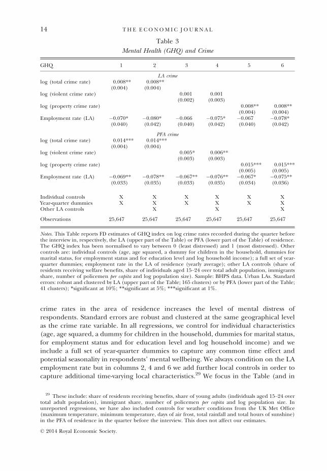
crime rates in the area of residence increases the level of mental distress ofrespondents. Standard errors are robust and clustered at the same geographical levelas the crime rate variable. In all regressions, we control for individual characteristics(age, age squared, a dummy for children in the household, dummies for marital status,for employment status and for education level and log household income) and weinclude a full set of year-quarter dummies to capture any common time effect andpotential seasonality in respondents’ mental wellbeing. We always condition on the LAemployment rate but in columns 2, 4 and 6 we add further local controls in order tocapture additional time-varying local characteristics.29 We focus in the Table (and in

Table 3

Mental Health (GHQ) and Crime

GHQ 1 2 3 4 5 6

LA crimelog (total crime rate) 0.008** 0.008**

(0.004) (0.004)log (violent crime rate) 0.001 0.001

(0.002) (0.003)log (property crime rate) 0.008** 0.008**

(0.004) (0.004)Employment rate (LA) �0.070* �0.080* �0.066 �0.075* �0.067 �0.078*

(0.040) (0.042) (0.040) (0.042) (0.040) (0.042)

PFA crimelog (total crime rate) 0.014*** 0.014***

(0.004) (0.004)log (violent crime rate) 0.005* 0.006**

(0.003) (0.003)log (property crime rate) 0.015*** 0.015***

(0.005) (0.005)Employment rate (LA) �0.069** �0.078** �0.067** �0.076** �0.067* �0.075**

(0.033) (0.035) (0.033) (0.035) (0.034) (0.036)

Individual controls X X X X X XYear-quarter dummies X X X X X XOther LA controls X X X

Observations 25,647 25,647 25,647 25,647 25,647 25,647

Notes. This Table reports FD estimates of GHQ index on log crime rates recorded during the quarter beforethe interview in, respectively, the LA (upper part of the Table) or PFA (lower part of the Table) of residence.The GHQ index has been normalised to vary between 0 (least distressed) and 1 (most distressed). Othercontrols are: individual controls (age, age squared, a dummy for children in the household, dummies formarital status, for employment status and for education level and log household income); a full set of year-quarter dummies; employment rate in the LA of residence (yearly average); other LA controls (share ofresidents receiving welfare benefits, share of individuals aged 15–24 over total adult population, immigrantsshare, number of policemen per capita and log population size). Sample: BHPS data. Urban LAs. Standarderrors: robust and clustered by LA (upper part of the Table; 165 clusters) or by PFA (lower part of the Table;41 clusters); *significant at 10%; **significant at 5%; ***significant at 1%.

29 These include: share of residents receiving benefits, share of young adults (individuals aged 15–24 overtotal adult population), immigrant share, number of policemen per capita and log population size. Inunreported regressions, we have also included controls for weather conditions from the UK Met Office(maximum temperature, minimum temperature, days of air frost, total rainfall and total hours of sunshine)in the PFA of residence in the quarter before the interview. This does not affect our estimates.



the reminder of the article) on estimates obtained for urban areas only, where theupper part and lower part of the Table report coefficient estimates of the (log) crimerate in the LA and PFA of residence respectively (both measured in the quarter beforethe interview).30

The point estimates reported in the first two columns in the upper part of Table 3suggest a positive impact in LA log total crime on individual mental distress. Thecoefficient is significant at the 5% level; inclusion of additional LA controls (column 2)does not affect the estimate. When we separate violent (columns 3 and 4) and propertycrime (columns 5 and 6), the estimated coefficients on both types of crime are positivebut the coefficient on violent crime is substantially smaller and not significantlydifferent from zero. The coefficient on property crime is identical to the one estimatedfor total crime and statistically significant. Thus, these results suggest that local crimeaffects mental well-being of residents in urban areas and that the effect is driven mainlyby property crime.

How large are these effects? The average value of the GHQ index is 0.31 withan overall standard deviation of 0.15 and a within-individual standard deviation of0.1 (see Table 1). Thus, and assuming linearity, an estimated coefficient of 0.008means that a 1 SD increase in log total crime rate (or property crime rate) causes a2.6% increase in the GHQ index. It explains about 5.3% of its overall standarddeviation and 8% of its within-individual standard deviation. This is a sizeableimpact.

In the lower part of Table 3, we report estimates where crime rates are measuredat the PFA level. The estimated coefficients are now larger in magnitude and moresignificant. We find that 1 SD increase in PFA log total crime causes a 0.014increase in individual mental distress of residents (or 4.5%). The coefficient issignificant at the 1% level even when all the additional LA controls are included inthe regression. The coefficient on property crime is of similar magnitude andstrongly significant. These regressions also show that violent crime in the areareduces mental well-being of residents: the coefficient estimate is about 0.005�0.006and significant. One reason for the larger estimates when using PFAs is that themental distress of people is related to changes in crime in an area larger than thelocal authority of residence. Indeed, as we discuss above, individuals may respond toproperty and violent crime outside their immediate residence area because theycommute to work or they socialise outside their residence LA. Moreover, forrelatively rare criminal offences such as violent crime, changes in local crime ratesmay be hardly observables for local residents who may instead look at larger areasin forming their expectations about victimisation risk. In both cases, measuringcrime on LA level may simply be too a small measure of neighbourhood crime topick up harmful effects through mental distress. In fact, it is easy to see thatincluding crime rates on LA level, if what matters for mental distress are crime rateson PFA level, will lead to an underestimate of the effect of crime, while including

30 We do not find a significant relationship between the GHQ index and area crime rates in rural areas,which may be related to the far lower crime rates in these areas (see Table 1), the lower population densityand the therefore lower variation in crime over time.



crime rates at PFA level, if what matters are crime rates at LA level, will not lead toa bias.31 Thus, throughout the article, we mainly focus on PFA crime rates.

To gain further insight on the magnitude of these effects, we compare theestimated effects with those of the local employment rate on residents’ mentalwell-being. The coefficient estimates in the last row show that changes in the localemployment rate are significantly, and negatively, associated with changes inmental distress of residents. The estimated coefficients suggest that a 10 percentagepoints increase in local employment rate improves residents’ mental health byabout 8% of its within-individual standard deviation. Thus, a 1 SD reduction in theLA (PFA) log total crime rate improves residents’ mental distress by roughly thesame amount as a 10 (20) percentage points increase in the local employment rate.Given that the standard deviation of the local employment rate is just 5 percentagepoints, the impact of a 1 SD decrease in the crime rate on mental health is abouttwice to four times as large as a 1 SD increase in the local employment rate.

Further comparisons can be made by looking at the estimated coefficientson individual controls (reported in Table A6 in the Appendix). Consistently withthe literature on the impact of major individual life events (getting married,divorcing, having a baby, being laid off etc.) on individual happiness (see, amongothers: Clark et al., 2008; Frijters et al., 2011; Clark and Georgellis, 2013), we findstrong and negative short-run effects on mental well-being of losing a partner,becoming unemployed or suffering a disabling injury. According to our estimates,the effect of a 1 SD increase in the local crime rate on mental distress is about one-seventh to one-fifth of the short-run effect of becoming unemployed. This is quitesubstantial, in particular when considering that the estimates for local crime ratesare the average effects for all residents, while the effects of changes in personalcircumstances relate only to those who are affected.

We report some robustness checks in Table A7, where we include, alternatively,a linear trend at the PFA level (columns 2) and at the LA level (columns 3).In addition, we test whether initial conditions in mental health, crime rates andother controls matter for the empirical relation we uncover. For each LA in oursample, we have computed initial average crime rates (total, property andviolent) in year 2002. Moreover, for the period 1999–2001, we compute theaverage GHQ score, averages of all BHPS individual controls and averages of all LAcontrols used in the main specification. In column 4 to 7 of Table A7, weprogressively include these baseline LA controls interacted with year dummies inour estimating equation. In columns 8 and 9, we alternatively add to these controlsa PFA and a LA linear trend. The estimates are remarkably similar across all thesespecifications.

31 To see that, consider the equation CRLA = CRPFA + dLA-PFA, where CRLA, CRPFA are crime rates on LAand PFA level, and dLA-PFA captures within-PFA variation in crime rates. Thus, dLA-PFA can be thought of as aresidual when regressing CRLA on a set of PFA dummies, which makes it immediately clear that it is notcorrelated with CRPFA. In this special case, erroneously using CRPFA as regressor while CRLA should be usedwill lead to unbiased estimates, as the measurement error dLA-PFA is not correlated with the included regressorCRPFA; however, using CRLA as a regressor when CRPFA is the correct measure of area crime will lead to adownward bias in estimates. See also Wooldridge (2002, p. 74).



3.2. Decomposing Mental Distress Measures

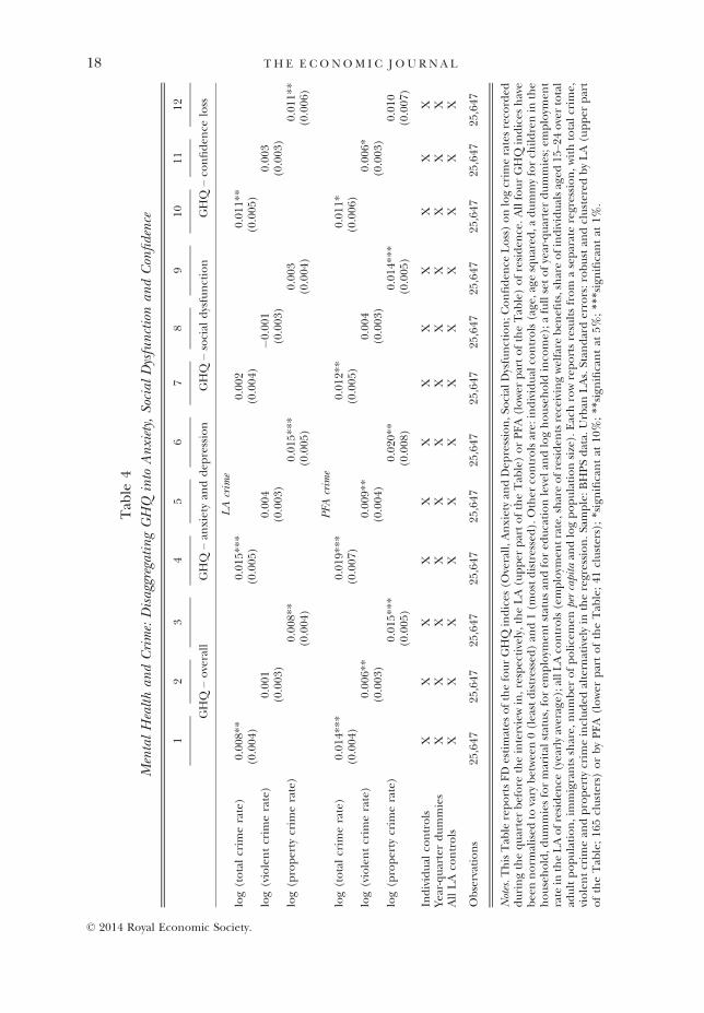
We now address the question whether the overall impact of local crime on mentaldistress established above is related to increased levels of anxiety and depression, orloss of self-confidence or social functionality. To do that, we use the disaggregatedindicators GHQ-Anxiety and Depression, GHQ-Social Dysfunction and GHQ-Confi-dence Loss (see Appendix A.1.1). In Table 4, we report estimates for the specificationthat include all controls.

If anything, one would expect exposure to crime to induce stress and anxiety, and toreduce the capability of enjoying daily activities. This direct effect could then reduceself-confidence and social interaction. Indeed, Stafford et al. (2007) find thatindividuals with pronounced fear of crime are twice as likely to suffer from depressionas individuals who are less concerned about crime. In line with this, our estimates showa strong adverse effect of local crime on the level of anxiety and depression ofresidents. The other two dimensions – social dysfunction and confidence loss – are alsoaffected but to a lesser extent. As before, the effects seem to be mainly driven byproperty crime and estimates are larger when aggregating data up on PFA level. At thataggregation level, violent crime has also an effect on anxiety and depression as well ason confidence loss, although smaller in magnitude.32

3.3. Different Crime Types

Our data distinguish between ten different categories of crime.33 This allows us toinvestigate more specifically which type of crime causes mental distress to residents. Forthe overall GHQ and its three sub-components, using the PFA aggregation, we reportestimation results in Table A9. We find strong effects on mental health of almost allproperty crime types, such as burglary, criminal damage, vehicle crime and ‘othertheft’, which all significantly increase the level of mental distress of residents in thearea. These types of crime account together for about 70% of total recorded crime inthe UK (see Table 2).34 Moreover, we find a clear detrimental effect of violence on themental health of people. Violence is by far the most frequent crime type in the category‘violent crime’, accounting for more than 86% of the total (Table 2). The non-significant effects of robbery and sexual crime need to be interpreted bearing in mindthat these are extremely rare events. Indeed, these two criminal offences togetheraccount for less than 3% of total recorded crime: on average, only 3 (5) individuals per10 thousand population are victims of sexual offences (robberies) in each quarter.

32 We have also broken down the GHQ index into its 12 components. Eight out of 12 of them aresignificantly affected by local crime rates at the PFA level, with a detrimental impact of crime on the ability toconcentrate, the perception of playing a useful role in life, the feeling of being constantly under strain, theability to overcome difficulties, the enjoyment of daily activities, the feeling of being depressed, the sense ofworthiness and the level of happiness (see Table A8).

33 These are: burglary, criminal damage, drug offences, fraud and forgery, offences against vehicles, othertheft offences, robbery, sexual offences, violence against the person and other offences (see Table A5 forcrime definitions).

34 ‘Fraud and forgery’, although having a positive coefficient, is non-significant. One reason could be thatthis type of crime is recorded where the victims reside but has no clear connection with the localenvironment (like e.g. credit card forgery).



Tab

le4

MentalHealthan

dCrime:DisaggregatingGHQ

into

Anxiety,Social

Dysfunctionan

dConfidence

12

34

56

78

910

1112

GHQ

–overall

GHQ

–an

xietyan

ddep

ression

GHQ

–social

dysfunction

GHQ

–co

nfiden

celoss

LAcrime

log(totalcrim

erate)

0.00

8**

0.01

5***

0.00

20.01

1**

(0.004

)(0.005

)(0.004

)(0.005

)log(violentcrim

erate)

0.00

10.00

4�0

.001

0.00

3(0.003

)(0.003

)(0.003

)(0.003

)log(p

roperty

crim

erate)

0.00

8**

0.01

5***

0.00

30.01

1**

(0.004

)(0.005

)(0.004

)(0.006

)

PFA

crime

log(totalcrim

erate)

0.01

4***

0.01

9***

0.01

2**

0.01

1*(0.004

)(0.007

)(0.005

)(0.006

)log(violentcrim

erate)

0.00

6**

0.00

9**

0.00

40.00

6*(0.003

)(0.004

)(0.003

)(0.003

)log(p

roperty

crim

erate)

0.01

5***

0.02

0**

0.01

4***

0.01

0(0.005

)(0.008

)(0.005

)(0.007

)

Individual

controls

XX

XX

XX

XX

XX

XX

Year-quarterdummies

XX

XX

XX

XX

XX

XX

AllLAco

ntrols

XX

XX

XX

XX

XX

XX

Observations

25,647

25,647

25,647

25,647

25,647

25,647

25,647

25,647

25,647

25,647

25,647

25,647

Notes.ThisTab

lereportsFDestimates

ofthefourGHQ

indices

(Overall,A

nxietyan

dDep

ression,S

ocial

Dysfunction;C

onfiden

ceLoss)onlogcrim

eratesreco

rded

duringthequarterbefore

theinterviewin,respectively,theLA(u

pper

partoftheTab

le)orPFA(lower

partoftheTab

le)ofresiden

ce.AllfourGHQ

indices

have

bee

nnorm

alised

tovary

betwee

n0(leastdistressed)an

d1(m

ostdistressed).Other

controlsare:

individual

controls(age

,age

squared

,adummyforch

ildrenin

the

household,dummiesformarital

status,forem

ploym

entstatusan

dfored

ucationlevelan

dloghousehold

inco

me);afullsetofyear-quarterdummies;em

ploym

ent

rate

intheLAofresiden

ce(yearlyaverage);allLAco

ntrols(employm

entrate,shareofresiden

tsreceivingwelfare

ben

efits,shareofindividualsaged

15–2

4overtotal

adultpopulation,im

migrantsshare,

number

ofpolicemen

percapita

andlogpopulationsize).Eachrowreportsresultsfrom

aseparateregression,withtotalcrim

e,violentcrim

ean

dproperty

crim

eincluded

alternativelyin

theregression.Sample:BHPSdata.

Urban

LAs.Stan

darderrors:robustan

dclustered

byLA(u

pper

part

oftheTab

le;16

5clusters)

orbyPFA(lower

partoftheTab

le;41

clusters);*significantat

10%;**sign

ificantat

5%;**

*significantat

1%.



When the GHQ index is decomposed into its three sub-factors, we find – as before –the largest effects on the anxiety and depression index.

3.4. Heterogeneous Effects of Crime

Different individuals may respond to crime in different ways. Indeed, both actual crimerisk and fear of crime are socially stratified, with some social groups being moreaffected than others. Some research suggests that women and the elderly are moreconcerned about crime (Lagrange and Ferraro, 1989), possibly because they feelparticularly vulnerable (Smith and Torstensson, 1997). The more educated may alsobe more aware of changes in local crime rates and, therefore, react more. On the otherhand, insofar as their higher level of education reflects their income group, they maybe less exposed to criminal hazard. The presence of children in the household may bean additional reason of added mental distress through area crime for parents andolder relatives. To investigate whether responses are heterogeneous along thesedimensions, we interact area crime rates with observed individuals characteristics andreport results in Table 5.

We find a clear gender dimension in the impact of exposure to crime on mentalhealth.35 While a 1 SD increase in log total crime causes an increase of 0.008 pointsin the overall GHQ index for men, the effect on women is more than twice aslarge. Breaking crime down into violent crime and property crime shows that theeffects of property crime are similar to those of total crime, with an effect onfemale residents which is exactly twice as large as those on males. Moreover, theeffects of violent crime discussed earlier are driven only by females, with a 1 SDincrease in the violent crime rate increasing women’s overall GHQ index by about0.008 points.

We have also investigated whether the effect of crime is more/less pronounced forthose under 30, over 65, with a higher education, or living in household with children.As the estimates in Table 5 show, these interaction terms are mostly non-significant,while the gender heterogeneity is robust to their inclusion.

3.5. The Timing of the Effect of Crime on Mental Distress

Our indices of mental health are subjective and self-reported measures that refer tointerviewees’ assessment as to how they felt around the time of the interview alongdifferent dimension of mental well-being.36 So far, we have shown that exposure tocrime shocks in the quarter before the interview leads to lower mental well-being ofresidents. One important question is whether the effect of crime on mental distressfades away quickly, or whether it causes more persistent mental distress.

We now investigate whether previous lags of local crime rates produce asignificant effect on current mental well-being. In addition, we test the robustness

35 This finding is consistent, for instance, with Frijters et al. (2011) who demonstrate that life satisfaction ofAustralian women is more strongly affected by (property) crime than that of men.

36 All 12 GHQ questions use the following wording: ‘Have you recently . . . felt/been/etc.?’ (see Table A1).



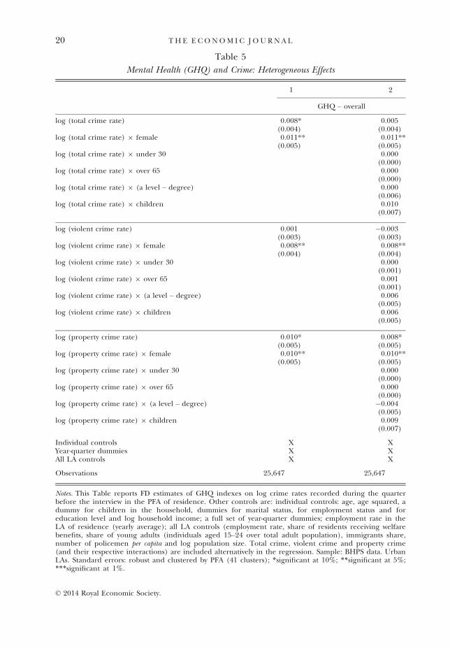
Table 5

Mental Health (GHQ) and Crime: Heterogeneous Effects

1 2

GHQ – overall

log (total crime rate) 0.008* 0.005(0.004) (0.004)

log (total crime rate) 9 female 0.011** 0.011**(0.005) (0.005)

log (total crime rate) 9 under 30 0.000(0.000)

log (total crime rate) 9 over 65 0.000(0.000)

log (total crime rate) 9 (a level – degree) 0.000(0.006)

log (total crime rate) 9 children 0.010(0.007)

log (violent crime rate) 0.001 �0.003(0.003) (0.003)

log (violent crime rate) 9 female 0.008** 0.008**(0.004) (0.004)

log (violent crime rate) 9 under 30 0.000(0.001)

log (violent crime rate) 9 over 65 0.001(0.001)

log (violent crime rate) 9 (a level – degree) 0.006(0.005)

log (violent crime rate) 9 children 0.006(0.005)

log (property crime rate) 0.010* 0.008*(0.005) (0.005)

log (property crime rate) 9 female 0.010** 0.010**(0.005) (0.005)

log (property crime rate) 9 under 30 0.000(0.000)

log (property crime rate) 9 over 65 0.000(0.000)

log (property crime rate) 9 (a level – degree) �0.004(0.005)

log (property crime rate) 9 children 0.009(0.007)

Individual controls X XYear-quarter dummies X XAll LA controls X X

Observations 25,647 25,647

Notes. This Table reports FD estimates of GHQ indexes on log crime rates recorded during the quarterbefore the interview in the PFA of residence. Other controls are: individual controls: age, age squared, adummy for children in the household, dummies for marital status, for employment status and foreducation level and log household income; a full set of year-quarter dummies; employment rate in theLA of residence (yearly average); all LA controls (employment rate, share of residents receiving welfarebenefits, share of young adults (individuals aged 15–24 over total adult population), immigrants share,number of policemen per capita and log population size. Total crime, violent crime and property crime(and their respective interactions) are included alternatively in the regression. Sample: BHPS data. UrbanLAs. Standard errors: robust and clustered by PFA (41 clusters); *significant at 10%; **significant at 5%;***significant at 1%.



of our results to a straightforward – but powerful – falsification exercise, byregressing current mental health status on future crime.

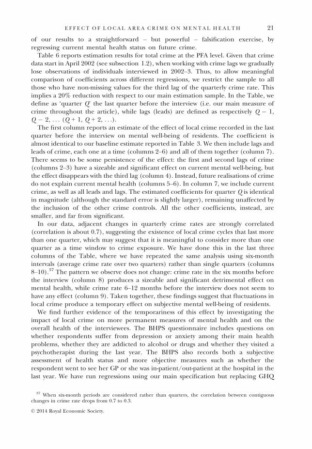
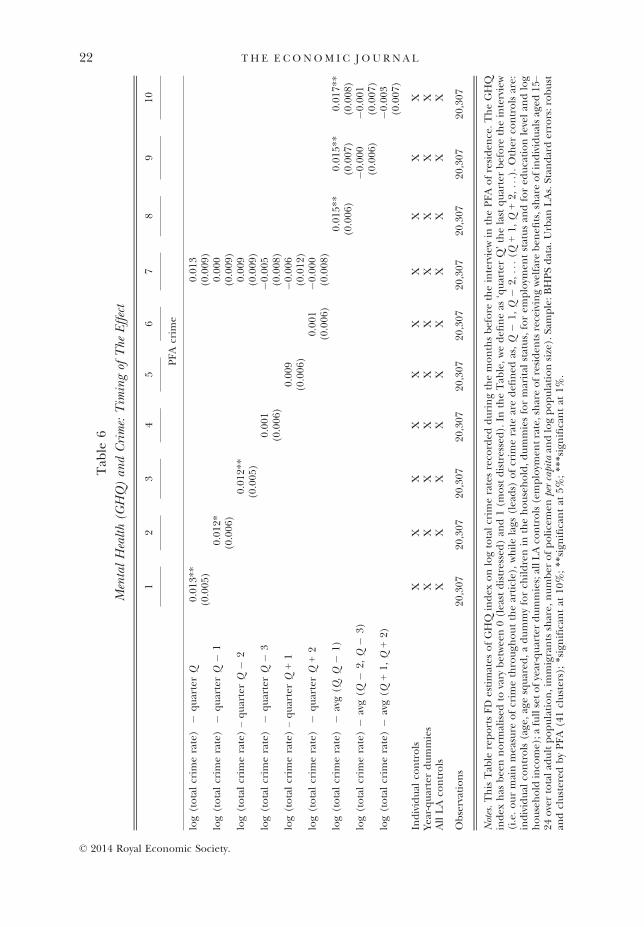
Table 6 reports estimation results for total crime at the PFA level. Given that crimedata start in April 2002 (see subsection 1.2), when working with crime lags we graduallylose observations of individuals interviewed in 2002–3. Thus, to allow meaningfulcomparison of coefficients across different regressions, we restrict the sample to allthose who have non-missing values for the third lag of the quarterly crime rate. Thisimplies a 20% reduction with respect to our main estimation sample. In the Table, wedefine as ‘quarter Q’ the last quarter before the interview (i.e. our main measure ofcrime throughout the article), while lags (leads) are defined as respectively Q � 1,Q � 2, . . . (Q + 1, Q + 2, . . .).

The first column reports an estimate of the effect of local crime recorded in the lastquarter before the interview on mental well-being of residents. The coefficient isalmost identical to our baseline estimate reported in Table 3. We then include lags andleads of crime, each one at a time (columns 2–6) and all of them together (column 7).There seems to be some persistence of the effect: the first and second lags of crime(columns 2–3) have a sizeable and significant effect on current mental well-being, butthe effect disappears with the third lag (column 4). Instead, future realisations of crimedo not explain current mental health (columns 5–6). In column 7, we include currentcrime, as well as all leads and lags. The estimated coefficients for quarter Q is identicalin magnitude (although the standard error is slightly larger), remaining unaffected bythe inclusion of the other crime controls. All the other coefficients, instead, aresmaller, and far from significant.

In our data, adjacent changes in quarterly crime rates are strongly correlated(correlation is about 0.7), suggesting the existence of local crime cycles that last morethan one quarter, which may suggest that it is meaningful to consider more than onequarter as a time window to crime exposure. We have done this in the last threecolumns of the Table, where we have repeated the same analysis using six-monthintervals (average crime rate over two quarters) rather than single quarters (columns8–10).37 The pattern we observe does not change: crime rate in the six months beforethe interview (column 8) produces a sizeable and significant detrimental effect onmental health, while crime rate 6–12 months before the interview does not seem tohave any effect (column 9). Taken together, these findings suggest that fluctuations inlocal crime produce a temporary effect on subjective mental well-being of residents.

We find further evidence of the temporariness of this effect by investigating theimpact of local crime on more permanent measures of mental health and on theoverall health of the interviewees. The BHPS questionnaire includes questions onwhether respondents suffer from depression or anxiety among their main healthproblems, whether they are addicted to alcohol or drugs and whether they visited apsychotherapist during the last year. The BHPS also records both a subjectiveassessment of health status and more objective measures such as whether therespondent went to see her GP or she was in-patient/out-patient at the hospital in thelast year. We have run regressions using our main specification but replacing GHQ

37 When six-month periods are considered rather than quarters, the correlation between contiguouschanges in crime rate drops from 0.7 to 0.3.



Tab

le6

MentalHealth(G

HQ)an

dCrime:Timingof

The

Effect

12

34

56

78

910

PFAcrim

e

log(totalcrim

erate)

�quarterQ

0.01

3**

0.01

3(0.005

)(0.009

)log(totalcrim

erate)

�quarterQ

�1

0.01

2*0.00

0(0.006

)(0.009

)log(totalcrim

erate)–quarterQ

�2

0.01

2**

0.00

9(0.005

)(0.009

)log(totalcrim

erate)

�quarterQ

�3

0.00

1�0

.005

(0.006

)(0.008

)log(totalcrim

erate)–quarterQ

+1

0.00

9�0

.006

(0.006

)(0.012

)log(totalcrim

erate)

�quarterQ

+2

0.00

1�0

.000

(0.006

)(0.008

)log(totalcrim

erate)

�avg(Q

,Q

�1)

0.01

5**

0.01

5**

0.01

7**

(0.006

)(0.007

)(0.008

)log(totalcrim

erate)�

avg(Q

�2,

Q�

3)�0

.000

�0.001

(0.006

)(0.007

)log(totalcrim

erate)�

avg(Q

+1,

Q+2)

�0.003

(0.007

)

Individual

controls

XX

XX

XX

XX

XX

Year-quarterdummies

XX

XX

XX

XX

XX

AllLAco

ntrols

XX

XX

XX

XX

XX

Observations

20,307

20,307

20,307

20,307

20,307

20,307

20,307

20,307

20,307

20,307

Notes.ThisTab

lereportsFD

estimates

ofGHQ

index

onlogtotalcrim

eratesreco

rded

duringthemonthsbefore

theinterviewin

thePFAofresiden

ce.TheGHQ

index

has

bee

nnorm

alised

tovary

betwee


d1(m

ostdistressed).In

theTab

le,wedefi

neas

‘quarterQ’thelastquarterbefore

theinterview

(i.e.ourmainmeasure

ofcrim

ethrough

outthearticle),whilelags

(leads)

ofcrim

erate

aredefi

ned

as,Q

�1,

Q�

2,...(Q

+1,

Q+2,

...).Other

controlsare:

individual

controls(age

,agesquared

,adummyforch

ildrenin

thehousehold,dummiesformarital

status,forem

ploym

entstatusan

dfored

ucationlevelan

dlog

household

inco

me);a

fullsetofyear-quarterdummies;allLAco

ntrols(employm


tsreceivingwelfare

ben

efits,shareofindividualsaged

15–

24overtotalad

ultpopulation,im

migrantsshare,

number

ofpolicemen

percapita

andlogpopulationsize).Sample:BHPSdata.

Urban

LAs.Stan

darderrors:robust

andclustered

byPFA(41clusters);*significantat

10%;**sign

ificantat

5%;**

*significantat

1%.



indices with each of these outcomes as dependent variable. We find no significantrelationship between any of these outcomes and crime rates recorded in the last three, sixor twelve months before the interview. Estimation results can be provided upon request.

All this evidence points at exposure to crime being a stressful but temporary event,which creates mental distress in the short run but has no immediate repercussions onmore permanent mental conditions, subjective health or attendance of health services.The temporariness of the effect we identify is fully consistent with the existingliterature on well-being which shows that individuals tend to adapt fairly quickly tomajor individual life events such as getting married, divorcing, having a baby, beinglaid off, etc., see for instance work by Clark et al. (2008), Frijters et al. (2011) and Clarkand Georgellis (2013). However, temporariness of the effects does not imply thatexposure to crime in the area of residence can be disregarded. Rather, although areacrime may not have persistent effects on mental distress, it is a repeated shock:different from other personal lifetime events that occur rarely, residents arepermanently exposed to temporary crime shocks. Even if individuals fully recoverafter each shock, this implies that in any given period there will be a sizeable fraction ofthe population – those living in areas hit by negative crime shocks – who is morementally distressed than in the absence of such shocks. This may have importantconsequences for their behaviour, relationships and productivity.38

3.6. Results Using the English Longitudinal Study of Ageing

We now turn to the data from the ELSA, focusing on people aged 50 and above. ELSAcontains two alternative measures of mental well-being: a depression index (PSH), anda measure of quality of life of older adults (CASP-19). To check the robustness of ourresults, we replicate our previous analysis using this alternative data set and measures ofmental well-being.39

Table 7 reports FD estimates of regressing the PSH and the CASP-19 indices on localcrime in the LA (upper part of the Table) or PFA (lower part of the Table) ofresidence. In spite of the differences in data, sample and measure of mental distress,our empirical findings are fully consistent with our previous results. Local crimeincreases mental distress of residents, with property crime seemingly playing a largerrole. In particular, the depression index PSH is significantly higher for individualsexposed to higher crime: a 1 SD increase in total crime in the LA of residence increasesthe PSH index by 0.024 points. This implies a 12% increase with respect to its meanvalue (0.2) and would explain up to 17% of its within-individual standard deviation(0.14). Similarly, a 1 SD increase in crime raises the CASP index by 0.008 points, whichcorresponds to a 3% increase with respect to its mean value (0.27) and to 13% of its

38 Although our setting does not allow us to identify the cumulative impact of having being exposed torepeated temporary crime shocks, the evidence from the MTO experiment, shows that moving away fromdeprived areas – that is, areas where individuals are more exposed to crime shocks – leads to significantimprovements in both subjective and objective well-being (Katz et al., 2001; Kling et al., 2007; Ludwig et al.,2012).

39 Given the age profile of the respondents, residential mobility is almost non-existent in the ELSA dataset: in each period, between 0% and 0.3% of interviewees have changed LA of residence with respect to theprevious wave.



within-individual standard deviation (0.06). Very similar coefficients are found for PFAcrime rates.

In unreported regressions, we have looked at which specific crime types produce thestrongest negative impact on resident mental well-being. Consistently with the evidencefrom the BHPS data discussed above (subsection 3.3), we find the largest and moresignificant coefficients for burglary, vehicle crime and violence.40

3.7. Assessing the Magnitude of Crime Effects

How large is the effect of being exposed to exogenous changes in local crime rates onindividuals’ mental health? We gave a first answer to this question by comparing ourestimates with the impact of the local employment rate (see subsection 3.1), and theimpact of changes in personal circumstances, such as becoming unemployed. In thissubsection, we investigate this aspect further, by contrasting the effects of changes in

Table 7

Mental Health and Crime: Evidence from ELSA

1 2 3 4 5 6

PSH CASP-19

LA crimelog (total crime rate) 0.024** 0.008**

(0.010) (0.004)log (violent crime rate) 0.013* 0.001

(0.007) (0.003)log (property crime rate) 0.018* 0.008**

(0.009) (0.003)

PFA crimelog (total crime rate) 0.024** 0.006

(0.010) (0.006)log (violent crime rate) 0.016** 0.002

(0.007) (0.004)log (property crime rate) 0.019* 0.003

(0.010) (0.006)

Individual controls X X X X X XYear-quarter dummies X X X X X XAll LA controls X X X X X X

Observations 10,816 10,816 10,816 7,825 7,825 7,825

Notes. This Table reports FD estimates of PSH and CASP-19 indexes on log crime rates recorded during thequarter before the interview in the LA (upper part of the Table) or PFA (lower part of the Table) of residence.Both indices have been normalised to vary between 0 (least distressed) and 1 (most distressed). Other controlsare: individual controls (age, age squared, a dummy for children in the household, dummies for maritalstatus, for employment status and for education level and log household income); a full set of year-quarterdummies; employment rate in the LA of residence (yearly average); all LA controls (employment rate, shareof residents receiving welfare benefits, share of individuals aged 15–24 over total adult population, immigrantsshare, number of policemen per capita and log population size). Each row reports estimation results fromseparate regressions, with each type of crime included alternatively in the regression. Sample: ELSA data.Urban LAs. Standard errors: robust and clustered by LA (upper part of the Table; 165 clusters) or by PFA(lower part of the Table; 41 clusters); *significant at 10%; **significant at 5%; ***significant at 1%.

40 Results can be provided upon request.



local crime rates to the effect to a major violent terrorist attack which had a dramaticimpact on the UK: the 7 July 2005 London bombings. This was a series of coordinatedsuicide attacks on London’s public transport system during the morning rush hours.The different explosions killed 52 people and injured about 700. The attacks werecompletely unexpected and represented the first terrorist act of Muslim extremists inthe UK. The impact of this event on British residents was quite dramatic.41

The BHPS data allow us to investigate the impact the 7/7 attack had on UKresidents’ self-reported mental health, as interviews are carried out throughout theentire year, so that, in 2005, some individuals have been interviewed before, and someafter, that event. Unfortunately, the immediate period before and after the terroristattack is not covered by the data, as interviews routinely stop in May and start again inSeptember (see Table A10). We make use of a difference-in-differences (DID)approach to identify the effect of interest. A similar identification strategy has beenimplemented with BHPS data by Metcalfe et al. (2011) to estimate the effect of theSeptember 11 attacks on the subjective well-being of the British population.

We identify the causal impact of the London bombings on British citizens’ mentalhealth by comparing those interviewed in the months preceding the bombing withthose interviewed in the months following the event. Our identification strategyassumes that the timing of the interview – with respect to the date of the Londonbombings – is random. A first concern arises from the possibility that interviewerscould manipulate the date of their interview in response to the London bombings.This seems unlikely as the terrorist attack – by definition – was unexpected and there isno reason to expect it to have affected the scheduled timings of BHPS interviews.42 Inany case, if individuals more negatively affected by the 7/7 attack refused to answer theBHPS questionnaire in the months after the event, we would estimate a lower bound ofthe overall effect. A second, more relevant, problem with this identification strategy isseasonality in responses: mental distress may differ in different months during the year.If autumn and winter months have a detrimental effect on mental well-being, then atleast part of the increase in mental distress after the 7/7 bombings could be driven bythis seasonal effect. We remove these effects by combining the before-after analysiswith a DID approach, comparing the difference in 2005 (before and after July) withthat measured in the year before (2004).43 We thus estimate the following regression:

MDit ¼ b0 þ b1AfterJulyi þ b2year2005t þ b3ðAfterJuly � year2005Þit þ vit : (2)

Here,MDit is the level of mental distress of individual i at time t. We identify the treatedgroup with a dummy variable Year2005 which is equal to one if the interview was carriedout in 2005 (rather than in 2004). The ‘treatment’ dummy AfterJuly, instead, is equal toone if the interview took place after July. The coefficient of interest is b3, which is equalto one for those individuals interviewed between September and December in 2005

41 Rubin et al. (2005, 2007) illustrate the impact on stress and perceived threat as well as travel behaviouramong Londoners in the aftermath of the event. Similar negative effects on mental well-being have beenobserved among the American population after the 9/11 attacks (Stein et al., 2004).

42 In addition, BHPS does not carry out interviews during the summer (Table A10). Thus, the possibledisruptions in the interview schedule by the terrorist attack in its immediate aftermath are not a concern here.

43 Including year 2003 does not substantially alter our findings. We do not use years after 2005, becausepermanent changes – such as the permanently higher levels of alert described in the previous Section – mayconfound the effects.



(that is, in the aftermath of the bombing). As before, we use as dependent variable themental well-being measured by GHQ (or by its sub-components: anxiety, socialdysfunction and confidence). Alternatively, we use the residuals from regressing GHQmeasures on individual characteristics, local authority fixed effects and year and monthdummies.44 Our design should randomise individuals across all these characteristics.Indeed, using either measure leads to basically the same results, which is what onewould expect if respondents’ characteristics are orthogonal with respect to the date ofthe interview. In all regressions, we cluster the standard errors by local authority ofresidence to allow for any possible correlation in the mental distress shocks ofindividuals living in the same area.

We report results of our DID estimates in Table 8. We start by looking at all LAs. Wethen progressively restrict the sample to the main 20 cities (in terms of population),the main five cities and, finally, Greater London (which contains 33 local authori-ties).45 In each case, our dependent variable is first the GHQ index and then theresidual GHQ. In the third column of each sample, we restrict the observations ofthose interviewed ‘after July’ only to the interviews collected in September (rather thanusing the period September-December).46 In the last three columns, instead, we lookat the three (residual) GHQ subcategories (still using only individuals interviewed inSeptember in the ‘after July’ group).

In all regressions, we find a positive coefficient on b3, suggesting that, in theaftermath of the London bombings, individuals reported a higher level of mental dis-tress. The coefficient increases in size and becomes strongly significant when we restrictthe sample to the main 20 cities, the main five cities or just London. Thus, the impactof the London bombings is larger on urban residents who are more exposed to the riskof a terrorist attack. Results for GHQ or residual GHQ are almost identical, as areresults we obtain when we drop individuals interviewed between October andDecember. Finally, columns 3–6 show that most of the impact seems to be on anxietyand depression. This is similar to the results we find for overall crime. There are alsosizeable effects on Social Dysfunction but no significant effect on Confidence Loss –again, similar to what we find for local area crime.

When we focus on the main five cities and on Greater London, in the monthsimmediately following the bombing, the self-reported mental distress increased byroughly 0.1 points, implying that the GHQ index increased by more than 30% withrespect to its mean value (which is about 0.3); this accounts for about 65% of itsstandard deviation (and for 100% of its within standard deviation).

How large are the effects of crime changes in the area of residence in comparison tothose we find for the London bombings? We report above that a 1 SD increase in log

44 As in our previous analysis, individual controls are: gender, age, age squared, a dummy for children inthe household, dummies for marital status, employment status, categorical variables for education level andlog household income.

45 The main 20 cities are: Birmingham, Bradford, Bristol, Cardiff, Coventry, Derby, Kingston-upon-Hull,Leeds, Leicester, Liverpool, London, Manchester, Newcastle upon Tyne, Nottingham, Plymouth, Sheffield,Southampton, Stoke-on-Trent, Swansea and Wolverhampton. The main five cities are: Birmingham,Bradford, Leeds, London and Sheffield.

46 The limited simple size of those interviewed in the first six month of the year, does not allow us torestrict the control group only to individuals interviewed in May (see Table A10).



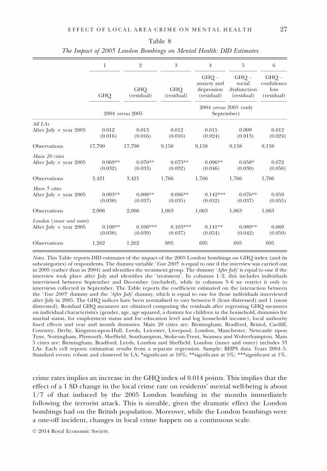
crime rates implies an increase in the GHQ index of 0.014 points. This implies that theeffect of a 1 SD change in the local crime rate on residents’ mental well-being is about1/7 of that induced by the 2005 London bombing in the months immediatelyfollowing the terrorist attack. This is sizeable, given the dramatic effect the Londonbombings had on the British population. Moreover, while the London bombings werea one-off incident, changes in local crime happen on a continuous scale.

Table 8

The Impact of 2005 London Bombings on Mental Health: DID Estimates

1 2 3 4 5 6

GHQGHQ

(residual)GHQ

(residual)

GHQ –anxiety anddepression(residual)

GHQ –social

dysfunction(residual)

GHQ –confidence

loss(residual)

2004 versus 20052004 versus 2005 (only

September)

All LAsAfter July 9 year 2005 0.012 0.013 0.012 0.015 0.009 0.012

(0.016) (0.016) (0.016) (0.024) (0.013) (0.024)

Observations 17,790 17,790 9,158 9,158 9,158 9,158

Main 20 citiesAfter July 9 year 2005 0.069** 0.070** 0.073** 0.096** 0.058* 0.072

(0.032) (0.033) (0.032) (0.046) (0.030) (0.058)

Observations 3,421 3,421 1,766 1,766 1,766 1,766

Main 5 citiesAfter July 9 year 2005 0.093** 0.098** 0.096** 0.142*** 0.076** 0.059

(0.038) (0.037) (0.035) (0.052) (0.037) (0.055)

Observations 2,006 2,006 1,063 1,063 1,063 1,063

London (inner and outer)After July 9 year 2005 0.100** 0.106*** 0.103*** 0.141** 0.089** 0.069

(0.038) (0.039) (0.037) (0.054) (0.042) (0.059)

Observations 1,262 1,262 695 695 695 695

Notes. This Table reports DID estimates of the impact of the 2005 London bombings on GHQ index (and itssubcategories) of respondents. The dummy variable ‘Year 2005’ is equal to one if the interview was carried outin 2005 (rather than in 2004) and identifies the treatment group. The dummy ‘After July’ is equal to one if theinterview took place after July and identifies the ‘treatment’. In columns 1–2, this includes individualsinterviewed between September and December (included), while in columns 3–6 we restrict it only tointerviews collected in September. The Table reports the coefficient estimated on the interaction betweenthe ‘Year 2005’ dummy and the ‘After July’ dummy, which is equal to one for those individuals interviewedafter July in 2005. The GHQ indices have been normalised to vary between 0 (least distressed) and 1 (mostdistressed). Residual GHQ measures are obtained computing the residuals after regressing GHQ measureson individual characteristics (gender, age, age squared, a dummy for children in the household, dummies formarital status, for employment status and for education level and log household income), local authorityfixed effects and year and month dummies. Main 20 cities are: Birmingham, Bradford, Bristol, Cardiff,Coventry, Derby, Kingston-upon-Hull, Leeds, Leicester, Liverpool, London, Manchester, Newcastle uponTyne, Nottingham, Plymouth, Sheffield, Southampton, Stoke-on-Trent, Swansea and Wolverhampton. Main5 cities are: Birmingham, Bradford, Leeds, London and Sheffield. London (inner and outer) includes 33LAs. Each cell reports estimation results from a separate regression. Sample: BHPS data. Years 2004–5.Standard errors: robust and clustered by LA; *significant at 10%; **significant at 5%; ***significant at 1%.



4. Conclusions

In this article, we analyse the indirect and intangible costs of crime, through inflictingmental distress, depression and anxiety, on individuals who live or work in the vicinitywhere crime takes place. We exploit detailed panel data on mental well-being from twolongitudinal surveys and we find that local crime rates have a significant, negative andsubstantial effect on mental well-being in urban areas. While most of this effect worksthrough property crime, violent crime turns out to be important when we increase thearea within which crime is recorded. This suggests that – while property crime concernsindividuals mostly when committed in their immediate neighbourhood – violent crimeis also relevant for the mental distress of citizens when it takes place in a larger spatialarea around their habitation. We benchmark our results with the impact on mentalhealth of British citizens of local unemployment rates, and the London bombings inJuly 2005. We show that the effect of a 1 SD increase in the crime rate on mental healthis about twice to four times as large as a 1 SD increase in the local employment rate;and about one-seventh of the impact of the London bombings – which was a dramaticevent. We conclude that the effects of local crime on mental distress of citizens arelarge, with possibly significant economic costs. Thus, crime reduction and crimeprevention may have benefits far beyond those typically suggested.

Appendix A. Additional Information

A.1. Measures of Mental Health

A.1.1. BHPS: The General Health Questionnaire (GHQ-12)The GHQ-12 questionnaire administered in the BHPS is as shown in Table A1.

While the longer versions of the GHQ are normally considered multidimensional, the GHQ-12 is often regarded as measuring only a single dimension of psychological health. However,several authors suggested that the GHQ-12 contained two or three clinically meaningful factors.Following Graetz’s (1991) disaggregation of GHQ-12 into three factors – (a) anxiety anddepression; (b) social dysfunction; (c) loss of confidence) – GHQ-12 questions can be grouped inthe following way (Table A2).

Table A1

GHQ-12 Questionnaire

Have you recently. . .. (1) Been able to concentrate on whatever you are doing?(2) Lost much sleep over worry?(3) Felt that you were playing a useful part in things?(4) Felt capable of making decisions about things?(5) Felt constantly under strain?(6) Felt that you could not overcome your difficulties?(7) Been able to enjoy your normal day-to-day activities?(8) Been able to face up to your problems?(9) Been feeling unhappy and depressed?(10) Been losing self-confidence in yourself?(11) Been thinking of yourself as a worthless person?(12) Been feeling reasonably happy, all things considered?

Answer Less than usual/no more than usual/rather more than usual/much morethan usual



A.1.2. Measures of Mental Health in ELSA

A.1.2.1. ELSA Psychosocial Health Module (PSH)The ELSA Psychosocial Health Module (PSH) assesses symptoms of depression, based on theCentre for Epidemiologic Studies Depression Scale (CES-D), which is one of the most commonscreening tests for helping an individual to determine his or her depression quotient (Radloff,1977). Interviewees are asked whether they recently had symptoms of depression (feeling ofunhappiness, loneliness, fatigue etc.). An index of depression can be constructed by assigningone point for each positive answer (and zero for negative ones). The measure ranges between 0(least distressed) and 8 (most distressed). In our empirical analysis, we normalise the variable torange between 0 (least distressed) and 1 (most distressed).

The PSH questions in ELSA are shown in Table A3.

A.1.2.2. CASP-19The ELSA contains also a theory-based measure of the quality of life of older adults whichconsists of 19 questions (CASP-19). Although this latter measure is not exactly conceived as anindex of mental well-being, it measures perceived general well-being of respondents whichshould reflect also their level of mental distress. Indeed, the type of questions asked to measureGHQ, PSH and CASP-19 are very similar in nature.

CASP-19 is a theory-based measure of the quality of life of older adults (Hyde et al., 2003),which consists of 19 questions (CASP-19). Although this latter measure is not exactly conceivedas an index of mental well-being, it measures perceived general well-being of respondents whichshould reflect also their level of mental distress. Indeed, the type of questions asked to measure

Table A2

GHQ-12 Disaggregation

Anxiety and depression (2) Lost much sleep over worry?(5) Felt constantly under strain?(6) Felt that you could not overcome your difficulties?(9) Been feeling unhappy and depressed?

Social dysfunction (1) Been able to concentrate on whatever you are doing?(3) Felt that you were playing a useful part in things?(4) Felt capable of making decisions about things?(7) Been able to enjoy your normal day-to-day activities?(8) Been able to face up to your problems?(12) Been feeling reasonably happy, all things considered?

Loss of confidence (10) Been losing self-confidence in yourself?(11) Been thinking of yourself as a worthless person?

Table A3

Psychosocial Health Module (PSH)

Much of the time during the past week . . . (1). . . have you felt depressed?(2). . . you felt that everything you did was an effort?(3). . . your sleep was restless?(4). . . you were happy?(5). . . you felt lonely?(6). . . you enjoyed life?(7). . . you felt sad?(8). . . you could not get going?

Answer: Yes/no



GHQ, PSH and CASP-19 are very similar in nature (compare Tables A1, A3, and A4). The CASP-19 questions cover four theoretical domains:

(i) control: the ability to intervene actively in one’s own environment;(ii) autonomy: the feeling of an individual to be free from unwanted interference by others;(iii) self-realisation: the active processes of human fulfilment; and(iv) pleasure: the sense of fun derived from the more active aspects of life.

The CASP-19 measure takes account of whether or how often (often, sometimes, not often ornever) statements on the four domains of quality of life apply to older people. A scale is createdthat ranges from 0, which represents total satisfaction on all domains, to 57, which represents acomplete absence of quality of life. In our empirical analysis, we adopt the Likert scoring methodand we normalise the variable to range between 0 (least distressed) and 1 (most distressed). TheCASP-19 questionnaire is shown in Table A4.

A.2. Identification and Empirical Issues

We estimate the following regression, where, we have written the region index r as a function ofthe individual i and time t, and where the dependent variable dMDir ði;tÞt are the residuals aftertime changing region and individual characteristics, and time dummies have been netted out:

gMDir ði;tÞt ¼ a0 þ a1CRr ði;tÞt þ LAr ði;tÞ þ gi þ uir ði;tÞt ; (A.1)

Suppose we estimate this equation in first differences. For individuals who do not move acrossLAs, the FD transformation removes both the LA and individual fixed effects:

DgMDir ði;tÞt ¼ a1DCRr ði;tÞt þ Duir ði;tÞt : (A.2)

The parameter a1 can be consistently estimated given that cov(ΔCRr(i,t)t, Δuir(i,t)t) = 0.For individuals who moved from region r to region r0, instead, we have:

gMDir 0ði;tÞt � gMDirði;t�1Þt�1 ¼ a1ðCRr 0ði;tÞt � CRrði;t�1Þt�1Þ þ ½eir 0ði;tÞt � eirði;t�1Þt�1�; (A.3)

where: eir 0 ði;tÞt ¼ LAr 0ði;tÞ þ uir 0 ði;tÞt and eir(i,t�1)t�1 = LAr(i,t�1) + uir(i,t�1)t�1.

Table A4

CASP-19

Control (1) My age prevents me from doing the things I would like to(2) I feel that what happens to me is out of my control(3) I feel free to plan for the future(4) I feel left out of things

Autonomy (5) I can do the things that I want to do(6) Family responsibilities prevent me from doing what I want to do(7) I feel that I can please myself what I do(8) My health stops me from doing things I want to do(9) Shortage of money stops me from doing the things I want to do

Pleasure (10) I look forward to each day(11) I feel that my life has meaning(12) I enjoy the things that I do(13) I enjoy being in the company of others(14) On balance, I look back on my life with a sense of happiness

Self-realisation (15) I feel full of energy these days(16) I choose to do things that I have never done before(17) I feel satisfied with the way my life has turned out(18) I feel that life is full of opportunities(19) I feel that the future looks good for me

Answer: Often/sometimes/not often/never



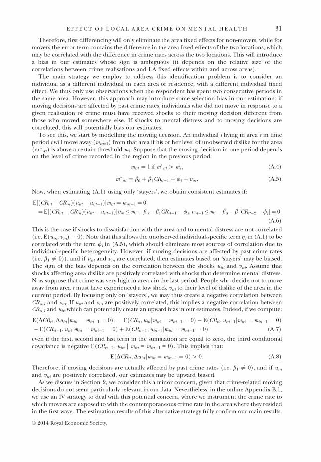
Therefore, first differencing will only eliminate the area fixed effects for non-movers, while formovers the error term contains the difference in the area fixed effects of the two locations, whichmay be correlated with the difference in crime rates across the two locations. This will introducea bias in our estimates whose sign is ambiguous (it depends on the relative size of thecorrelations between crime realisations and LA fixed effects within and across areas).

The main strategy we employ to address this identification problem is to consider anindividual as a different individual in each area of residence, with a different individual fixedeffect. We thus only use observations when the respondent has spent two consecutive periods inthe same area. However, this approach may introduce some selection bias in our estimation: ifmoving decisions are affected by past crime rates, individuals who did not move in response to agiven realisation of crime must have received shocks to their moving decision different fromthose who moved somewhere else. If shocks to mental distress and to moving decisions arecorrelated, this will potentially bias our estimates.

To see this, we start by modelling the moving decision. An individual i living in area r in timeperiod t will move away (mirt=1) from that area if his or her level of unobserved dislike for the area(m*irt) is above a certain threshold mi . Suppose that the moving decision in one period dependson the level of crime recorded in the region in the previous period:

mirt ¼ 1 if m�irt [mi ; (A.4)

m�irt ¼ b0 þ b1CRrt�1 þ /i þ virt : (A.5)

Now, when estimating (A.1) using only ‘stayers’, we obtain consistent estimates if:

E ðCRirt �CRirtÞðuirt �uirt�1Þjmirt ¼mirt�1 ¼ 0½ �¼ E ðCRirt �CRirtÞðuirt �uirt�1Þjvirt � �mi �b0�b1CRrt�1�/i ;virt�1� �mi½ �b0�b1CRrt�2�/i � ¼ 0:

(A.6)

This is the case if shocks to dissatisfaction with the area and to mental distress are not correlated(i.e. E(uirt, virt) = 0). Note that this allows the unobserved individual-specific term gi in (A.1) to becorrelated with the term /i in (A.5), which should eliminate most sources of correlation due toindividual-specific heterogeneity. However, if moving decisions are affected by past crime rates(i.e. b1 6¼ 0)), and if uirt and virt are correlated, then estimates based on ‘stayers’ may be biased.The sign of the bias depends on the correlation between the shocks uirt and virt. Assume thatshocks affecting area dislike are positively correlated with shocks that determine mental distress.Now suppose that crime was very high in area r in the last period. People who decide not to moveaway from area r must have experienced a low shock virt to their level of dislike of the area in thecurrent period. By focusing only on ‘stayers’, we may thus create a negative correlation betweenCRrt-1 and virt. If uirt and virt are positively correlated, this implies a negative correlation betweenCRrt-1 and uirt which can potentially create an upward bias in our estimates. Indeed, if we compute:

EðDCRrt ;Duirt jmirt ¼ mirt�1 ¼ 0Þ ¼ EðCRrt ;uirt jmirt ¼ mirt�1 ¼ 0Þ � EðCRrt ;uirt�1jmirt ¼ mirt�1 ¼ 0Þ� EðCRrt�1;uirt jmirt ¼ mirt�1 ¼ 0Þ þ EðCRrt�1;uirt�1jmirt ¼ mirt�1 ¼ 0Þ ðA:7Þeven if the first, second and last term in the summation are equal to zero, the third conditionalcovariance is negative E(CRrt�1, uirt | mirt = mirt�1 = 0). This implies that:

EðDCRrt ;Duirt jmirt ¼ mirt�1 ¼ 0Þ[ 0: (A.8)

Therefore, if moving decisions are actually affected by past crime rates (i.e. b1 6¼ 0), and if uirtand virt are positively correlated, our estimates may be upward biased.

As we discuss in Section 2, we consider this a minor concern, given that crime-related movingdecisions do not seem particularly relevant in our data. Nevertheless, in the online Appendix B.1,we use an IV strategy to deal with this potential concern, where we instrument the crime rate towhich movers are exposed to with the contemporaneous crime rate in the area where they residedin the first wave. The estimation results of this alternative strategy fully confirm our main results.



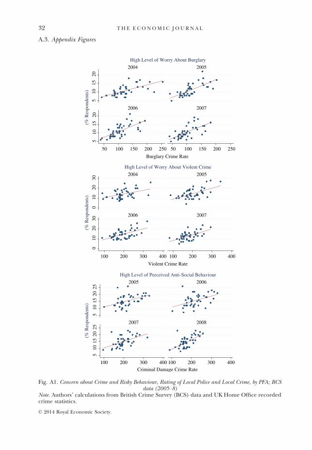
A.3. Appendix Figures

510

1520

510

1520

50 100 150 200 250 50 100 150 200 250

2004 2005

2006 2007

Burglary Crime Rate

High Level of Worry About Burglary

010

2030

010

2030

100 200 300 400 100 200 300 400

2004 2005

2006 2007

Violent Crime Rate

High Level of Worry About Violent Crime

510

1520

255

1015

2025

100 200 300 400 100 200 300 400

2005 2006

2007 2008

Criminal Damage Crime Rate

High Level of Perceived Anti-Social Behaviour

(% R

espo

nden

ts)

(% R

espo

nden

ts)

(% R

espo

nden

ts)

Fig. A1. Concern about Crime and Risky Behaviour, Rating of Local Police and Local Crime, by PFA; BCSdata (2005–8)

Note. Authors’ calculations from British Crime Survey (BCS) data and UK Home Office recordedcrime statistics.



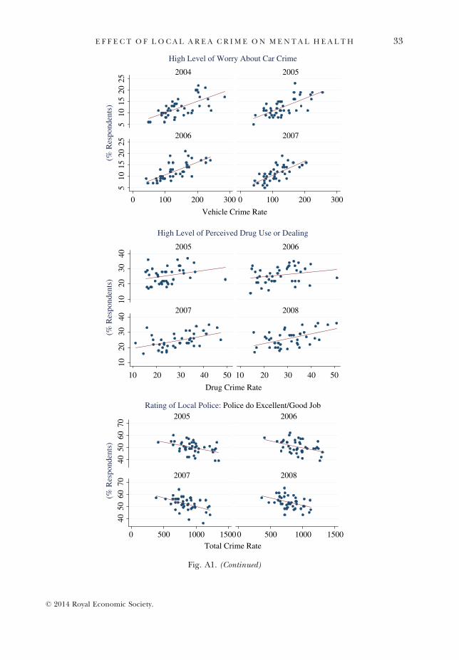
510

1520

255

1015

2025

0 100 200 300 0 100 200 300

2004 2005

2006 2007

Vehicle Crime Rate

High Level of Worry About Car Crime

1020

3040

1020

3040

10 20 30 40 50 10 20 30 40 50

2005 2006

2007 2008

Drug Crime Rate

High Level of Perceived Drug Use or Dealing

Rating of Local Police: Police do Excellent/Good Job

(% R

espo

nden

ts)

(% R

espo

nden

ts)

4050

6070

4050

6070

0 500 1000 15000 500 1000 1500

2005 2006

2007 2008

Total Crime Rate

(% R

espo

nden

ts)

Fig. A1. (Continued)



A.4. Appendix Tables

Table A5

Mental Health (GHQ) and Crime: Individual and LA Controls

GHQ – Overall1 2 3 4

LA crime PFA crime

log (total crime rate) 0.008** 0.008** 0.014*** 0.014***(0.004) (0.004) (0.004) (0.004

Marital status (excluded category: married/civil partnership)Separated 0.027* 0.026* 0.027* 0.027*

(0.015) (0.015) (0.015) (0.015)Divorced �0.008 �0.008 �0.008 �0.008

(0.011) (0.011) (0.010) (0.010)Widowed 0.070*** 0.070*** 0.070*** 0.070***

(0.016) (0.016) (0.020) (0.020)Never married 0.008 0.008 0.008 0.008

(0.009) (0.009) (0.010) (0.010)

Employment status (excluded category: employed)Self-employed 0.006 0.006 0.006 0.006

(0.006) (0.006) (0.006) (0.006)Unemployed 0.057*** 0.057*** 0.057*** 0.057***

(0.007) (0.007) (0.007) (0.007)Retired 0.012* 0.012* 0.012* 0.012*

(0.007) (0.007) (0.006) (0.006)Maternity leave �0.002 �0.002 �0.002 �0.002

(0.011) (0.011) (0.010) (0.010)Family care 0.027*** 0.027*** 0.027*** 0.027***

(0.007) (0.007) (0.005) (0.005)Full time student 0.009 0.009 0.009 0.009

(0.008) (0.008) (0.008) (0.008)Sick, disabled 0.064*** 0.064*** 0.064*** 0.064***

(0.011) (0.011) (0.010) (0.010)Government training scheme �0.005 �0.005 �0.006 �0.006

(0.033) (0.033) (0.020) (0.021)Other 0.037** 0.037** 0.037*** 0.037***

(0.014) (0.014) (0.013) (0.013)

LA controlsEmployment rate �0.070* �0.080* �0.069** �0.078**

(0.040) (0.042) (0.033) (0.035)Share of benefit claimants �0.434 �0.431

(0.380) (0.485)Share of residents aged 15–24 �0.688* �0.653*

(0.379) (0.375)Share of immigrants 0.062 0.068

(0.071) (0.060)Police officer per capita �0.506 �0.307

(0.594) (0.506)log (resident population) 0.014 �0.001

(0.133) (0.125)

Other individual controls X X X XYear-quarter dummies X X X XObservations 25,647 25,647 25,647 25,647

Notes. This Table reports FD estimates of GHQ index on log crime rates recorded during the quarter before theinterview in, respectively, the LA (columns 1–2) or PFA (columns 3–4) of residence. The GHQ index has beennormalised to vary between 0 (least distressed) and 1 (most distressed). ‘Other individual controls’ are: age, agesquared, a dummy for children in thehousehold, categorical variables for education level and loghousehold income.Sample: BHPS data. Urban LAs. Standard errors: robust and clustered by LA (upper part of the Table; 165 clusters)or by PFA (lower part of the Table; 41 clusters); *significant at 10%; **significant at 5%; ***significant at 1%.



Tab

leA6

MentalHealth(G

HQ)an

dCrime:Trends

andInitialConditions

12

34

56

78

9

LAcrime

log(totalcrim

erate)

0.00

8**

0.00

7*0.00

70.00

8**

0.00

8**

0.00

7*0.00

7*0.00

7*0.00

6(0.004

)(0.004

)(0.004

)(0.004

)(0.004

)(0.004

)(0.004

)(0.004

)(0.004

)

log(violentcrim

erate)

0.00

10.00

10.00

10.00

20.00

10.00

10.00

20.00

10.00

1(0.003

)(0.003

)(0.003

)(0.003

)(0.003

)(0.003

)(0.003

)(0.003

)(0.003

)

log(p

roperty

crim

erate)

0.00

8**

0.00

7*0.00

7*0.00

9**

0.00

8**

0.00

7*0.00

7*0.00

7*0.00

6(0.004

)(0.004

)(0.004

)(0.004

)(0.004

)(0.004

)(0.004

)(0.004

)(0.004

)

PFA

crime

log(totalcrim

erate)

0.01

4***

0.01

4***

0.01

3***

0.01

5***

0.01

5***

0.01

4***

0.01

4**

0.01

4**

0.01

3**

(0.004

)(0.005

)(0.005

)(0.005

)(0.005

)(0.005

)(0.006

)(0.006

)(0.006

)

log(violentcrim

erate)

0.00

6**

0.00

6*0.00

6*0.00

6**

0.00

6**

0.00

50.00

50.00

50.00

5(0.003

)(0.003

)(0.003

)(0.003

)(0.003

)(0.003

)(0.003

)(0.004

)(0.004

)

log(p

roperty

crim

erate)

0.01

5***

0.01

5**

0.01

4**

0.01

6***

0.01

6***

0.01

6***

0.01

5**

0.01

5**

0.01

5**

(0.005

)(0.006

)(0.005

)(0.005

)(0.005

)(0.005

)(0.006

)(0.007

)(0.007

)

PFAlineartren

dX

XLAlineartren

dX

XInitialLAcrim

erates

XX

XX

XX

InitialavgGHQ

(LA)

XX

XX

XInitialavgBHPSco

ntrols(L

A)

XX

XX

InitialLAco

ntrols

XX

XIndividual

controls

XX

XX

XX

XX

XYe

ar-quarterdummies

XX

XX

XX

XX

XAllLAco

ntrols

XX

XX

XX

XX

XObservations

25,647

25,647

25,647

25,647

25,635

25,635

24,661

24,661

24,661

Notes.ThisTab

lereportsFD

estimates

ofGHQ

index

onlogcrim

eratesreco

rded


theinterviewin,respectively,theLA(u

pper

partoftheTab

le)or

PFA(lower

partoftheTab

le)ofresiden

ce.TheGHQ

index

has

beennorm

alised

tovary

between0(leastdistressed)an

d1(m

ostdistressed).Alineartren

disincluded

atthe

PFAlevel(co

lumns2an

d8)

orat

theLAlevel(co

lumns3an

d9).‘InitialL

Acrim

erates’istheaveragecrim

erate

(respectively,total,propertyan

dviolent)in

theLAofresiden

cein

year

2002

interacted

withyear

dummies.‘InitialavgGHQ

(LA)’istheaverageGHQ

intheLAofresiden

cemeasuredovertheperiod19

99–2

001an

dinteracted

withyear

dummies.‘Initialavg

BHPSco

ntrols(L

A)’aretheaverages

ofindividualco

ntrolsin

theLAofresiden

cemeasuredovertheperiod19

99–2

001an

dinteracted

withyear

dummies.

‘InitialLA

controls’aretheaverageLAco

ntrolsmeasuredovertheperiod19

99–2

001an

dinteracted

withyear

dummies.Other

controlsare:

individual

controls(age

,age

squared

,adummyforch

ildrenin

thehousehold,dummiesformarital

status,forem

ploym

entstatusan

dfored

ucationlevel,an

dloghousehold

inco

me);afullsetofyear-

quarterdummies;em

ploym

entrate

intheLAofresiden

ce(yearlyaverage);allLAco

ntrols(employm


tsreceivingwelfare

ben

efits,shareofindividuals

aged

15–2

4overtotaladultpopulation,immigrantsshare,number

ofp

olicemen

percapitaan

dlogpopulationsize).Eachcellreportsresultsfrom

aseparateregression,w

ithtotal

crim

e,violentcrim

ean

dpropertycrim

eincluded

alternativelyin

theregression.S

ample:B

HPSdata.Urban

LAs.Stan

darderrors:robustan

dclustered

byLA(u

pper

partofthe

Tab

le;16

5clusters)

orbyPFA(lower

partoftheTab

le;41

clusters);*significantat

10%;**

sign

ificantat

5%;***significantat

1%.



Tab

leA7

MentalHealthan

dCrime:SingleGHQ

Item

s

GHQ

item

(1)Unab

leto

concentrate

(3)Notplaying

usefulrole

(5)Constan

tly

under

strain

(6)Unab

leto

overcome

difficu

lties

(7)Noten

joying

day-to-day

activities

(9)Fee

ling

unhap

pyor

dep

ressed

(11)

Fee

ling

worthless

(12)

Notfeeling

reasonab

lyhap

py

log(totalcrim

erate)

0.01

7*0.01

7**

0.01

6**

0.02

1***

0.01

7**

0.02

2**

0.01

2*0.01

6**

(0.008

)(0.008

)(0.007

)(0.007

)(0.007

)(0.010

)(0.007

)(0.006

)

log(violentcrim

erate)

0.00

50.00

50.00

40.01

1**

0.00

60.01

1**

0.00

7**

0.00

8**

(0.005

)(0.004

)(0.005

)(0.004

)(0.004

)(0.005

)(0.003

)(0.003

)

log(p

roperty

crim

erate)

0.02

0**

0.01

9**

0.01

9**

0.02

0**

0.01

7**

0.02

3*0.01

10.01

4**

(0.009

)(0.008

)(0.008

)(0.009

)(0.008

)(0.012

)(0.008

)(0.007

)

Individual

controls

XX

XX

XX

XX

Year-quarterdummies

XX

XX

XX

XX

AllLAco

ntrols

XX

XX

XX

XX

Observations

25,647

25,647

25,647

25,647

25,647

25,647

25,647

25,647

Notes.ThisTab

lereportsFDestimates

ofsingleGHQ

item

sonlogcrim

eratesreco

rded


theinterviewin

thePFAofresiden

ce.E

achofthe

GHQ

item

shas

bee

nnorm

alised

tovary

betwee


d1(m

ostdistressed).Other

controlsare:

individual

controls(age

,age

squared

,adummyfor

children

inthehousehold,dummiesformarital

status,

forem

ploym

entstatusan

dfored

ucation

levelan

dloghousehold

inco

me);afullsetofyear-quarter

dummies;

employm

entrate

intheLA

ofresiden

ce(yearlyaverage);allLA

controls

(employm


tsreceivingwelfare

ben

efits,shareof

individualsaged

15–2

4overtotalad

ultpopulation,im

migrantsshare,

number

ofpolicemen

percapita

andlogpopulationsize).Eachcellreportsestimationresults

from

aseparateregression.Sample:BHPSdata.

Urban

LAs.Stan

darderrors:robust

andclustered

byPFA(41clusters);*significantat

10%;**sign

ificantat

5%;

***significantat

1%.



Table A8

Mental Health and Crime: Different Crime Types

1 2 3 4

GHQ –overall

GHQ – anxietyand depression

GHQ – socialdysfunction

GHQ – confidenceloss

Total crimeViolent crimeln (robbery rate) 0.003 0.008 �0.001 0.003

(0.005) (0.008) (0.005) (0.010)

ln (sexual crime rate) �0.000 0.001 �0.002 0.002(0.003) (0.003) (0.003) (0.004)

ln (violence rate) 0.005** 0.007** 0.003 0.005**(0.002) (0.003) (0.003) (0.002)

Property crimeln (burglary rate) 0.012** 0.017** 0.010** 0.005

(0.004) (0.006) (0.004) (0.006)

ln (criminal damage rate) 0.006* 0.007 0.005 0.006(0.003) (0.005) (0.003) (0.005)

ln (fraud and forgery rate) 0.004 0.005 0.003 0.005(0.003) (0.005) (0.002) (0.005)

ln (vehicle crime rate) 0.008** 0.010 0.008* 0.003(0.004) (0.006) (0.004) (0.007)

ln (other theft rate) 0.014** 0.019** 0.013** 0.005(0.005) (0.007) (0.005) (0.007)

Other crimeln (drug crime rate) 0.001 0.001 0.001 0.001

(0.002) (0.003) (0.003) (0.004)

ln (any other crime rate) 0.004 0.006 0.001 0.008**(0.003) (0.004) (0.003) (0.004)

Individual controls X X X XYear-quarter dummies X X X XAll LA controls X X X X

Observations 25,647 25,647 25,647 25,647

Notes. This Table reports FD estimates of the four GHQ indices (Overall, Anxiety and Depression, SocialDysfunction; Confidence Loss) on log crime rates recorded during the quarter before the interview in thePFA of residence. All four GHQ indices have been normalised to vary between 0 (least distressed) and1 (most distressed). Other controls are: individual controls (age, age squared, a dummy for children in thehousehold, dummies for marital status, for employment status and for education level, and log householdincome); a full set of year-quarter dummies; employment rate in the LA of residence (yearly average); all LAcontrols (employment rate, share of residents receiving welfare benefits, share of individuals aged 15–24 overtotal adult population, immigrants share, number of policemen per capita and log population size). Each cellreports estimation results from a separate regression. Sample: BHPS data. Urban LAs. Standard errors: robustand clustered by PFA (41 clusters); *significant at 10%; **significant at 5%; ***significant at 1%.



University College London and CReAMQueen Mary University of London, CReAM and IZA

Submitted: 28 October 2013Accepted: 6 June 2014

Additional Supporting Information may be found in the online version of this article:

Appendix B. Alternative Channels and Further Results.Data S1.

ReferencesAcheson, D. (chaired by) (1998). ‘Independent inquiry into inequalities in health’, http://www.archive.

official-documents.co.uk/document/doh/ih/ih.htm (last accessed: 13 June 2014).Atkinson, G., Healey, A. and Mourato, S. (2005). ‘Valuing the costs of violent crime: a stated preference

approach’, Oxford Economic Papers, vol. 57(4), pp. 559–85.Becker, G. and Rubinstein, Y. (2011). ‘Fear and the response to terrorism: an economic analysis’, CEP

Discussion Paper No. 1079.Besley, T. and Mueller, H. (2012). ‘Estimating the peace dividend: the impact of violence on house prices in

Northern Ireland’, American Economic Review, vol. 102(2), pp. 810–33.Braakman, N. (2013). ‘How do individuals deal with victimization and victimization risk? Longitudinal

evidence from Mexico’, Journal of Economic Behavior and Organization, vol. 84(1), pp. 335–44.Carson, R.T. (2012). ‘Contingent valuation: a practical alternative when prices aren’t available’, Journal of

Economic Perspectives, vol. 26(4), pp. 27–42.Chadee, D., Austen, L. and Ditton, J. (2007). ‘The relationship between likelihood and fear of criminal

victimization: evaluating risk sensitivity as a mediating concept’, British Journal of Criminology, vol. 47(1),pp. 133–53.

Clark, A.E. (2003). ‘Unemployment as a social norm: psychological evidence from panel data’, Journal of LaborEconomics, vol. 21(2), pp. 289–322.

Clark, A.E., Diener, E., Georgellis, Y. and Lucas, R. (2008). ‘Lags and leads in life satisfaction: a test of thebaseline hypothesis’, ECONOMIC JOURNAL, vol. 118(529), pp. F222–43.

Clark, A. and Georgellis, Y. (2013). ‘Back to baseline in Britain: adaptation in the British household panelsurvey’, Economica, vol. 80(319), pp. 496–512.

Table A9

BHPS: Number of Interviews by Year and Month

Interview month Year 2004 Wave Year 2005 Wave Year 2006 Wave

January 84 14 167 15 131 16February 42 14 58 15 23 16March 17 14 12 15 19 16April 9 14 6 15 1 16May 0 14 3 15 0 16

Total (January–May) 152 246 174

September 4,168 15 4,952 16 5,226 17October 3,196 15 3,064 16 2,976 17November 1,291 15 931 16 789 17December 272 15 176 16 127 17

Total (September–December) 8,927 9,123 9,118

Note. Authors’ calculations from BHPS data.



Clark, A.E. and Oswald, A.J. (1994). ‘Unhappiness and unemployment’, ECONOMIC JOURNAL, vol. 104(424), pp.648–59.

Cohen, M.A., Rust, R.T., Steen, S. and Tidd, S.T. (2004). ‘Willingness to pay for crime control programs’,Criminology, vol. 42(1), pp. 89–109.

Cornaglia, F., Feldman, N.E. and Leigh, A. (2014). ‘Crime and mental wellbeing’, Journal of Human Resources,vol. 49(1), pp. 110–40.

CSDH. (2008). ‘Closing the gap in a generation: health equity through action on the social determinants ofhealth’, WHO – Commission on Social Determinants of Health.

Department of Health. (1999). Reducing Health Inequalities: An Action Report, London: Department of Health.Department of Health. (2009). Tackling Health Inequalities: 10 Years On. London: Department of Health.Diez-Roux, A.V. and Mair, C. (2010). ‘Neighbourhoods and health’, Annals of the New York Academy of the

Sciences, vol. 1186, The Biology of Disadvantage: Socioeconomic Status and Health, pp. 125–45.Dolan, P., Loomes, G., Peasgood, T. and Tsuchiya, A. (2005). ‘Estimating the intangible victim cost of violent

crime’, British Journal of Criminology, vol. 45(6), pp. 958–76.Dubourg, R., Hamed, J. and Thorns, J. (2005). ‘The economic and social costs of crime against individuals

and households 2003/04’, Home Office On-Line Report 30/05. http://webarchive.nationalarchives.gov.uk/20100413151441/http:/www.homeoffice.gov.uk/rds/pdfs05/rdsolr3005.pdf. date (last accessed: 01September 2013).

Ferraro, K. (1995). Fear of Crime: Interpreting Victimisation Risk, Albany, NY: SUNY Press.Frijters, P., Johnston, D.W. and Shields, M.A. (2011). ‘Life satisfaction dynamics with quarterly life event

data’, Scandinavian Journal of Economics, vol. 113(1), pp. 190–211.Gardner, J. and Oswald, A.J. (2007). ‘Money and mental wellbeing: a longitudinal study of medium-sized

lottery wins’, Journal of Health Economics, vol. 26(1), pp. 49–60.Gibbons, S. (2004). ‘The costs of urban property crime’, ECONOMIC JOURNAL, vol. 114(499), pp. F441–63.Goldberg, D. (1978). Manual of the General Health Questionnaire, Windsor: National Foundation.Gould, E.D., Weinberg, B.A. and Mustard, D.B. (2002). ‘Crime rates and local labor market opportunities in

the United States: 1979–1997’, The Review of Economics and Statistics, vol. 84(1), pp. 45–61.Graetz, B. (1991). ‘Multidimensional properties of the general health questionnaire’, Social Psychiatry and

Psychiatric Epidemiology, vol. 26(3), pp. 132–8.Green, G., Gilbertson, J.M. and Grimsley, M.F.J. (2002). ‘Fear of crime and health in residential tower blocks’,

European Journal of Public Health, vol. 12(1), pp. 10–15.Hale, C. (1996). ‘Fear of crime: a review of the literature’, International Review of Victimology, vol. 4(2), pp. 79–

150.Hamermesh, D.S. (1999). ‘Crime and the timing of work’, Journal of Urban Economics, vol. 45(2), pp. 311–30.Harrendorf, S., Heiskanen, M. and Malby, S. (edited by) (2010). ‘International statistics on crime and

justice’, HEUNI-UNDOC.Hausman, J. (2012). ‘Contingent valuation: from dubious to hopeless’, Journal of Economic Perspectives, vol. 26

(4), pp. 43–56.Hyde, M., Wiggins, R.D., Higgs, P. and Blane, D.B. (2003). ‘A measure of quality of life in early old age: the

theory, development and properties of a needs satisfaction model (CASP-19)’, Aging and Mental Health,vol. 7(3), pp. 186–94.

Jackson, J. and Stafford, M. (2009). ‘Public health and fear of crime: a prospective cohort study’, BritishJournal of Criminology, vol. 49(6), pp. 832–47.

Janke, K., Propper, C. and Shields, M.A. (2013). ‘Does violent crime deter physical activity?’, IZA DiscussionPapers 7545, Institute for the Study of Labor (IZA).

Katz, L.F., Kling, J.R. and Liebman, J.B. (2001). ‘Moving to opportunity in Boston: early results of arandomized mobility experiment’, Quarterly Journal of Economics, vol. 116(2), pp. 607–54.

Kling, J.R., Liebman, J.B. and Katz, L.F. (2007). ‘Experimental analysis of neighbourhood effects’,Econometrica, vol. 75(1), pp. 83–119.

Lagrange, R.L. and Ferraro, K.F. (1989). ‘Assessing age and gender differences in perceived risk and fear ofcrime’, Criminology, vol. 27(4), pp. 697–720.

Layard, R. (2005). ‘Mental health: Britain’s biggest social problem?’, presented at the No. 10 Strategy UnitSeminar on Mental Health, 20th January.

Linden, L. and Rockoff, J.E. (2008). ‘Estimates of the impact of crime risk on property values from meganlaw’, American Economic Review, vol. 98(3), pp. 1103–27.

Ludwig, J., Duncan, G.J., Gennetian, L.A., Katz, L.F., Kessler, R.C., Kling, J.R. and Sanbonmatsu, L. (2012).‘Neighborhood effects on the long-term well-being of low-income adults’, Science vol. 337 (6101), pp.1505–10.

Mair, C., Diez Roux, A.V. and Galea, S. (2008). ‘Are neighbourhood characteristics associated with depressivesymptoms? A review of evidence’, Journal of Epidemiology and Community Health, vol. 62(11), pp. 940–6.

Mawby, R. (1992). ‘Crime and the elderly: a review of British and American research’, Current PsychologicalReviews, vol. 2(3), pp. 301–10.



Metcalfe, R., Powdthavee, N. and Dolan, P. (2011). ‘Destruction and distress: using a quasi-experiment toshow the effects of the September 11 attacks on mental well-being in the United Kingdom’, ECONOMIC

JOURNAL, vol. 121(550), pp. F81–103.National Institute for Mental Health in England. (2005). ‘Making it possible: improving mental health and

well-being in England’, Leeds: National Institute for Mental Health in England.Oreopoulos, P. (2003). ‘The long-run consequences of living in a poor neighbourhood’, Quarterly Journal of

Economics, vol. 118(4), pp. 1533–75.Piccinelli, M., Bisoffi, G., Bon, M.G., Cunico, L. and Tansella, M. (1993). ‘Validity and test-retest reliability of

the Italian version of the 12-item general health questionnaire in general practice: a comparison betweenthree scoring methods’, Comprehensive Psychiatry, vol. 34(3), pp. 198–205.

Propper, C., Jones, K., Bolster, A., Burgess, S., Johnston, R. and Sarker, R. (2005). ‘Local neighbourhood andmental health: evidence from the UK’, Social Science and Medicine, vol. 61(10), pp. 2065–83.

Radloff, L.S. (1977). ‘The CES-D scale: a self-report depression scale for research in the general population’,Applied Psychological Measurement, vol. 1(3), pp. 385–401.

Raphael, S. and Winter-Ebmer, R. (2001). ‘Identifying the effect of unemployment on crime’, Journal of Lawand Economics, vol. 44(1), pp. 259–83.

Ross, C.E. and Mirowsky, J. (2001). ‘Neighbourhood disadvantage, disorder, and health’, Journal of Health andSocial Behaviour, vol. 42(3), pp. 258–76.

Rubin, G.J., Brewin, C.R., Greenberg, N., Simpson, J. and Wessely, S. (2005). ‘Psychological and behaviouralreactions to the bombings in London on 7 July 2005: cross sectional survey of a representative sample ofLondoners’, British Medical Journal, vol. 331(7517), pp. 606–11.

Rubin, G.J., Brewin, C.R., Greenberg, N., Simpson, J. and Wessely, S. (2007). ‘Enduring consequences ofterrorism: 7-month follow-up survey of reactions to the bombings in London on 7 July 2005’, BritishJournal of Psychiatry, vol. 190, pp. 350–6.

Smith, W.R. and Torstensson, M. (1997). ‘Gender differences in risk perception and neutralizing fear ofcrime: toward resolving the paradoxes’, British Journal of Criminology, vol. 37(4), pp. 608–34.

Soares, R.R. (2010). ‘Welfare costs of crime and common violence: a critical review’, Working Paper 581,Department of Economics PUC-Rio.

Stafford, M., Chandola, T. and Marmot, M. (2007). ‘Association between fear of crime and mental health andphysical functioning’, American Journal of Public Health, vol. 97(11), pp. 2076–81.

Stein, B.D., Elliott, M.N., Jaycox, L.H., Collins, R.L., Berry, S.H., Klein, D.J. and Schuster, M.A. (2004). ‘Anational longitudinal study of the psychological consequences of the September 11, 2001 terroristattacks: reactions, impairment, and help-seeking’, Psychiatry: Interpersonal and Biological Processes, vol. 67(2), pp. 105–17.

Whitley, R. and Prince, M. (2005). ‘Fear of crime, mobility and mental health in inner-city London, UK’,Social Science and Medicine, vol. 61(8), pp. 1678–88.

Wooldridge, J. (2002). Econometric Analysis of Cross Section and Panel Data, vol. 1, Cambridge MA: MIT Press



the effect of local area crime on mental healthuctpb21/cpapers/areacrimeandmentalhealth.pdfthe...

Documents