the effect of gender inequality in education on economic
TRANSCRIPT
BSc Thesis Economics and Business
The Effect of Gender Inequality in Education
on Economic Growth
in South-East Asia and the Pacific
Name:
Student ID:
Specialization:
Faculty:
Supervisor:
Date:
Charlotte M. L. van Leeuwen
11078200
Economics
Economics and Business
Ms. N. J. Leefmans
31/01/2018
2
Statement of Originality
This document is written by Student Charlotte van Leeuwen who declares to take full
responsibility for the contents of this document.
I declare that the text and the work presented in this document is original and that no sources
other than those mentioned in the text and its references have been used in creating it.
The Faculty of Economics and Business is responsible solely for the supervision of
completion of the work, not for the contents.
3
Abstract
Lately, gender inequality in a variety of areas has been an issue in many countries in this
world. One of the areas that should be addressed in developing countries is the gender bias in
education. This paper empirically investigates the effect of gender inequality in education on
economic growth using yearly panel data between 1960 and 2010 for a set of 20 countries
within South-East Asia and the Pacific. Results based on Ordinary Least Squares regressions
conclude that the gender inequality in education has a significant positive direct effect and a
significant negative indirect effect through the investment ratio, the life expectancy at birth
and the labour force share on economic growth. However, the negative indirect effects
outweigh the positive direct effect. As follows an increase the female-male ratio of average
years of schooling of 1 percentage point will lead to an increase of 0.0033 percentage point in
the gross domestic product per capita. This implies that decreasing gender inequality will
result in an increase in economic growth.
4
Table of contents
page
1. Introduction
2. Literature review
2.1 Determinants of economic growth
2.2 Gender inequality as determinant of economic growth
3. Data and research method
3.1 The model
3.2 Selection of variables
4. Descriptive statistics
5. Empirical results and analysis
5.1 Results for the basic model
5.2 Results for the model including time, country and region dummies
6. Conclusion
References
Appendix
5
9
9
13
14
17
19
21
22
24
26
JEL Codes: I2, J16, O4
5
1. Introduction
In the year 2000, eight Millennium Development Goals (MDGs) were established by
the United Nations with the overall purpose of reducing poverty (United Nations, 2015). The
191 member states of the UN and several international organizations committed to help
achieve these goals by 2015. The third MDG was the promotion of gender equality and
empowerment of women (United Nations, 2015). This goal is among other things the result
of what Sen called the “missing women”, referring to the excess mortality of women due to
gender inequality (Duflo, 2012). Since closing the gender inequality gap was on many states’
and organizations’ agenda, gender inequality did decline over the last decades (United
Nations, 2015). However, the year 2005 was the earliest date to achieve the third Millennium
Development Goal with its main target of ending gender disparities in primary and secondary
education. This target has been missed in more than 60% of countries for which data was
available (Unterhalter, 2006). Moreover, The Millennium Development Goals Report 2015
states that despite many successes, gender inequality persists. Women are still being
discriminated and more likely to live in poverty compared to men.
Gender inequality should change in different areas (Kabeer, 2005) such as with
respect to employment and politics. This paper will focus on the inequality in education.
Various studies (Kabeer, 2005) conclude that more educated women are more likely to use
contraception and antenatal care. It also increases the participation of women in a wider range
of decisions, their access to resources and their role in economic decision-making.
Furthermore, they seem less likely to suffer from domestic violence since they appear to be
better at dealing with violent partners. Overall, access to education increases women’s well-
being and capability to exercise control over their lives.
Besides closing gender gaps in education being a goal in itself, it can also be seen as
an instrument to achieve other objectives such as other development goals. It has been argued
that inequalities in education are significant concerns for human development and well-being
(D Hicks, 1997). Cooray and Potrafke (2011) state that the increase in education for girls has
a positive effect on children’s health and education through their educated mothers. Gender
inequality in education also affects the economic development and growth of a country
(Klasen, 2002; Cooray & Potrafke, 2011). Female education increases productivity (Knowles,
Lorgelly & Owen, 2002) and human capital (Cooray & Potrafke, 2011), through which it
affects economic growth.
6
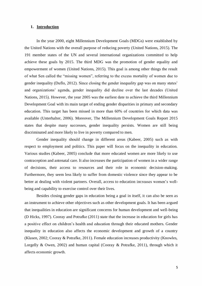
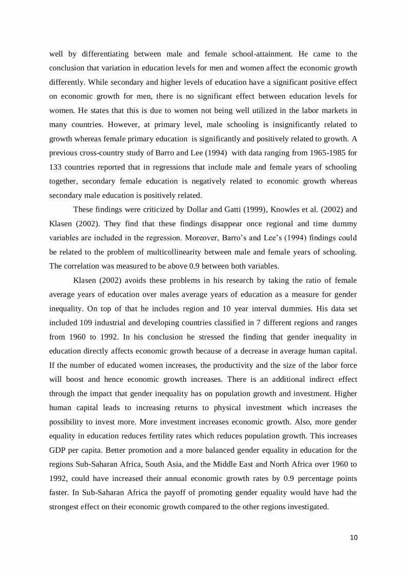
Stotsky, Shibuya and
Kebaj (2016) examined the
trends in gender equality and
women’s advancement for the
International Monetary Fund
(IMF). One of their findings
was that over a period from
1980 to 2014 the female to
male ratio of gross secondary
enrollment increased in all
regions. As can be seen in
figure 1, gender equality in
education improved for Africa,
Middle East & Central Asia, and Asia & the Pacific, where for the latter the improvement
was particularly large. In 2014, the ratio for Asia and the Pacific even exceeded Europe’s
ratio. Governments in South Asia are very engaged and successful in advancing basic
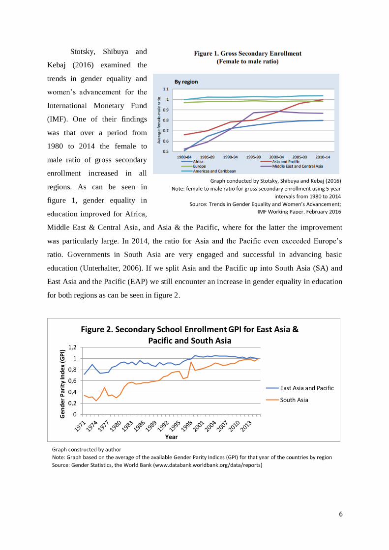
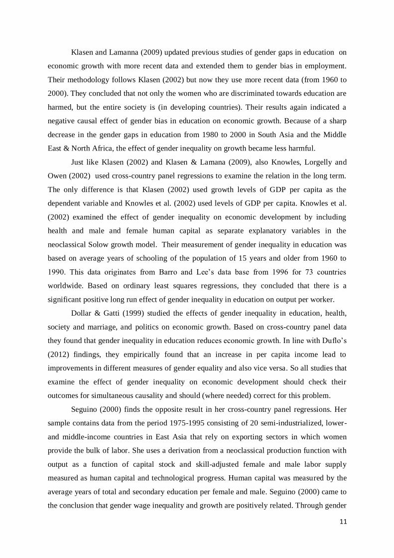
education (Unterhalter, 2006). If we split Asia and the Pacific up into South Asia (SA) and
East Asia and the Pacific (EAP) we still encounter an increase in gender equality in education
for both regions as can be seen in figure 2.
Graph constructed by author
Note: Graph based on the average of the available Gender Parity Indices (GPI) for that year of the countries by region
Source: Gender Statistics, the World Bank (www.databank.worldbank.org/data/reports)
Graph conducted by Stotsky, Shibuya and Kebaj (2016)
Note: female to male ratio for gross secondary enrollment using 5 year
intervals from 1980 to 2014
Source: Trends in Gender Equality and Women’s Advancement;
IMF Working Paper, February 2016
0
0,2
0,4
0,6
0,8
1
1,2
Gen
der
Par
ity
Ind
ex (
GP
I)
Year
Figure 2. Secondary School Enrollment GPI for East Asia & Pacific and South Asia
East Asia and Pacific
South Asia
7
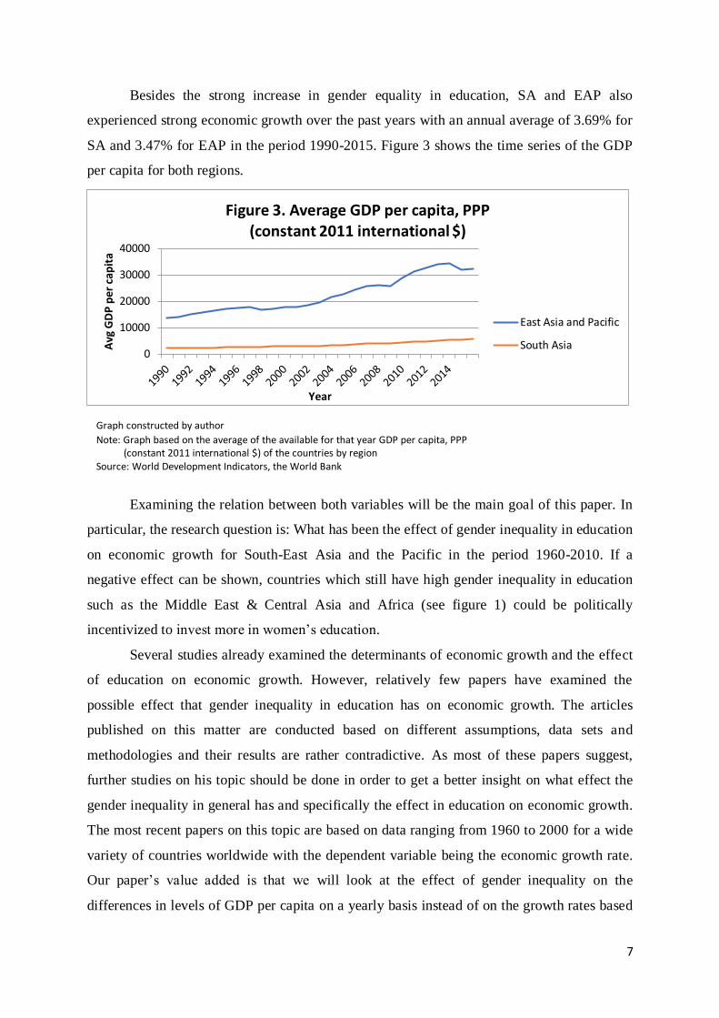
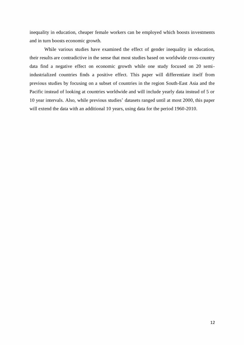
Besides the strong increase in gender equality in education, SA and EAP also
experienced strong economic growth over the past years with an annual average of 3.69% for
SA and 3.47% for EAP in the period 1990-2015. Figure 3 shows the time series of the GDP
per capita for both regions.
Examining the relation between both variables will be the main goal of this paper. In
particular, the research question is: What has been the effect of gender inequality in education
on economic growth for South-East Asia and the Pacific in the period 1960-2010. If a
negative effect can be shown, countries which still have high gender inequality in education
such as the Middle East & Central Asia and Africa (see figure 1) could be politically
incentivized to invest more in women’s education.
Several studies already examined the determinants of economic growth and the effect
of education on economic growth. However, relatively few papers have examined the
possible effect that gender inequality in education has on economic growth. The articles
published on this matter are conducted based on different assumptions, data sets and
methodologies and their results are rather contradictive. As most of these papers suggest,
further studies on his topic should be done in order to get a better insight on what effect the
gender inequality in general has and specifically the effect in education on economic growth.
The most recent papers on this topic are based on data ranging from 1960 to 2000 for a wide
variety of countries worldwide with the dependent variable being the economic growth rate.
Our paper’s value added is that we will look at the effect of gender inequality on the
differences in levels of GDP per capita on a yearly basis instead of on the growth rates based
0
10000
20000
30000
40000
Avg
GD
P p
er c
apit
a
Year
Figure 3. Average GDP per capita, PPP (constant 2011 international $)
East Asia and Pacific
South Asia
Graph constructed by author
Note: Graph based on the average of the available for that year GDP per capita, PPP (constant 2011 international $) of the countries by region Source: World Development Indicators, the World Bank
8
on 5 or 10 year intervals. We will also limit our study for the region South-East Asia and the
Pacific over a longer period (1960-2010). By combining methodologies from past papers,
previous findings will be investigated using Ordinary Least Squares (OLS) regressions.
The thesis is structured as follows. Previous literature and findings on the
determinants of economic growth and on gender inequality in education and its relation to
economic growth will be reviewed in section 2. In section 3 the research method and
variables used in the regressions will be specified. The descriptive statistics will be outlined
in section 4 and section 5 will analyze the results. In section 6 a sensitivity analysis will be
conducted to check the robustness of our findings and section 7 will end the paper with a
conclusion.
9
2. Literature review
Various papers have studied the relation and effects between gender inequality in
education and economic growth. However, their results do not always seem consistent with
each other. This might be due to differences in control variables, gender inequality measures,
sample data and/or methodologies. An overview of previous studies and their findings will be
discussed in this section.
2.1 Determinants of economic growth
The variables that affect economic growth have been widely studied. Often the
models to determine the effects on economic growth are either based on the neoclassical
growth theory (Romer, 2011) or on the endogenous growth theory (Barro, 2001).
The determinants of output per worker (growth) in the Solow growth model (based on
the neoclassical growth model) are the level of physical capital, human capital and the level
of technology. In the short run economic growth is also determined by conditional
convergence, meaning that countries with a low initial real income tend to grow faster
economically compared to rich countries. However, large variations in growth in the long run
– both across countries and over time – only occur from an increase in change in technology.
The latter is taken as exogenous in the model and could correspond to knowledge or to the
education levels and skills of the labor force. In other words, differences in education could
be the main driver of differences in economic growth in the long run according to the Solow
growth model.
Barro’s (2001) endogenous growth models include various variables that theoretically
can be linked to growth. In one of his studies he examined the role of human capital on
economic growth. His research was based on cross-country panel data for 100 countries
divided over 3 periods from 1965 to 1995 with initial level of GDP, government consumption
as a percentage of GDP, rule of law, international openness, inflation rate, fertility rate,
investment ratio, terms of trade and education being the exogenous variables.
2.2 Gender inequality in education as determinants for economic growth
Examining the effect of gender inequality in education as a determinant of economic
growth has been studied to a lesser extent. Barro (2001) however did examine the latter as
10
well by differentiating between male and female school-attainment. He came to the
conclusion that variation in education levels for men and women affect the economic growth
differently. While secondary and higher levels of education have a significant positive effect
on economic growth for men, there is no significant effect between education levels for
women. He states that this is due to women not being well utilized in the labor markets in
many countries. However, at primary level, male schooling is insignificantly related to
growth whereas female primary education is significantly and positively related to growth. A
previous cross-country study of Barro and Lee (1994) with data ranging from 1965-1985 for
133 countries reported that in regressions that include male and female years of schooling
together, secondary female education is negatively related to economic growth whereas
secondary male education is positively related.
These findings were criticized by Dollar and Gatti (1999), Knowles et al. (2002) and
Klasen (2002). They find that these findings disappear once regional and time dummy
variables are included in the regression. Moreover, Barro’s and Lee’s (1994) findings could
be related to the problem of multicollinearity between male and female years of schooling.
The correlation was measured to be above 0.9 between both variables.
Klasen (2002) avoids these problems in his research by taking the ratio of female
average years of education over males average years of education as a measure for gender
inequality. On top of that he includes region and 10 year interval dummies. His data set
included 109 industrial and developing countries classified in 7 different regions and ranges
from 1960 to 1992. In his conclusion he stressed the finding that gender inequality in
education directly affects economic growth because of a decrease in average human capital.
If the number of educated women increases, the productivity and the size of the labor force
will boost and hence economic growth increases. There is an additional indirect effect
through the impact that gender inequality has on population growth and investment. Higher
human capital leads to increasing returns to physical investment which increases the
possibility to invest more. More investment increases economic growth. Also, more gender
equality in education reduces fertility rates which reduces population growth. This increases
GDP per capita. Better promotion and a more balanced gender equality in education for the
regions Sub-Saharan Africa, South Asia, and the Middle East and North Africa over 1960 to
1992, could have increased their annual economic growth rates by 0.9 percentage points
faster. In Sub-Saharan Africa the payoff of promoting gender equality would have had the
strongest effect on their economic growth compared to the other regions investigated.
11
Klasen and Lamanna (2009) updated previous studies of gender gaps in education on
economic growth with more recent data and extended them to gender bias in employment.
Their methodology follows Klasen (2002) but now they use more recent data (from 1960 to
2000). They concluded that not only the women who are discriminated towards education are
harmed, but the entire society is (in developing countries). Their results again indicated a
negative causal effect of gender bias in education on economic growth. Because of a sharp
decrease in the gender gaps in education from 1980 to 2000 in South Asia and the Middle
East & North Africa, the effect of gender inequality on growth became less harmful.
Just like Klasen (2002) and Klasen & Lamana (2009), also Knowles, Lorgelly and
Owen (2002) used cross-country panel regressions to examine the relation in the long term.
The only difference is that Klasen (2002) used growth levels of GDP per capita as the
dependent variable and Knowles et al. (2002) used levels of GDP per capita. Knowles et al.
(2002) examined the effect of gender inequality on economic development by including
health and male and female human capital as separate explanatory variables in the
neoclassical Solow growth model. Their measurement of gender inequality in education was
based on average years of schooling of the population of 15 years and older from 1960 to
1990. This data originates from Barro and Lee’s data base from 1996 for 73 countries
worldwide. Based on ordinary least squares regressions, they concluded that there is a
significant positive long run effect of gender inequality in education on output per worker.
Dollar & Gatti (1999) studied the effects of gender inequality in education, health,
society and marriage, and politics on economic growth. Based on cross-country panel data
they found that gender inequality in education reduces economic growth. In line with Duflo’s
(2012) findings, they empirically found that an increase in per capita income lead to
improvements in different measures of gender equality and also vice versa. So all studies that
examine the effect of gender inequality on economic development should check their
outcomes for simultaneous causality and should (where needed) correct for this problem.
Seguino (2000) finds the opposite result in her cross-country panel regressions. Her
sample contains data from the period 1975-1995 consisting of 20 semi-industrialized, lower-
and middle-income countries in East Asia that rely on exporting sectors in which women
provide the bulk of labor. She uses a derivation from a neoclassical production function with
output as a function of capital stock and skill-adjusted female and male labor supply
measured as human capital and technological progress. Human capital was measured by the
average years of total and secondary education per female and male. Seguino (2000) came to
the conclusion that gender wage inequality and growth are positively related. Through gender
12
inequality in education, cheaper female workers can be employed which boosts investments
and in turn boosts economic growth.
While various studies have examined the effect of gender inequality in education,
their results are contradictive in the sense that most studies based on worldwide cross-country
data find a negative effect on economic growth while one study focused on 20 semi-
industrialized countries finds a positive effect. This paper will differentiate itself from
previous studies by focusing on a subset of countries in the region South-East Asia and the
Pacific instead of looking at countries worldwide and will include yearly data instead of 5 or
10 year intervals. Also, while previous studies’ datasets ranged until at most 2000, this paper
will extend the data with an additional 10 years, using data for the period 1960-2010.
13
3. Data and research methods
3.1 The model
This paper will examine both the direct and indirect effect of gender inequality in
education on economic development for the regions South-East Asia and the Pacific. The
direct effect will be measured by:
𝑙𝑛𝑔𝑑𝑝𝑐𝑎𝑝𝑖𝑡 = 𝛼1 + 𝛽1𝑙𝑛𝑔𝑑𝑝𝑐𝑎𝑝60𝑖 + 𝛽2𝐼𝑛𝑣𝑖𝑡−1 + 𝛽3𝑂𝑝𝑒𝑛𝑖𝑡 + 𝛽4𝐿𝐹𝑆𝑖𝑡 + 𝛽5𝐿𝐸 𝑖𝑡 +
𝛽6𝐸𝐷𝑖𝑡 + 𝛽7𝑅𝐸𝐷𝑖𝑡 + 𝛽8𝑋 + 휀 (1)
To test the indirect effects some additional tests and regressions will be run to
measure the effect of gender inequality on life expectancy, the investment ratio and the labor
force share respectively:
𝐿𝐸𝑖𝑡 = 𝛼2 + 𝛽9𝑅𝐸𝐷𝑖𝑡 + 𝜑 (2)
𝐼𝑛𝑣𝑖𝑡−1 = 𝛼3 + 𝛽10𝑂𝑝𝑒𝑛𝑖𝑡 + 𝛽11𝐿𝐹𝑆𝑖𝑡 + 𝛽12𝐸𝐷𝑖𝑡 + 𝛽13𝑅𝐸𝐷𝑖𝑡 + 𝛾 (3)
𝐿𝐹𝑆𝑖𝑡 = 𝛼4 + 𝛽14𝐸𝐷𝑖𝑡 + 𝛽15𝑅𝐸𝐷𝑖𝑡 + 𝛿 (4)
In these equations the dependent variable lngdpcap represents the natural logarithm of the
GDP per capita. The 𝛼’s are the constants of the regressions. The control variables in the
regressions are the following: Inv is the ratio of investment over GDP per capita; Open is the
measure for the openness to trade; LFS is the labor force share; LE measures the life
expectancy at birth; ED represents the average years of education and X is a measure for
regional, country and year dummy variable. Note that the dummy variable will only be used
in the sensitivity analysis in section 6. RED is the variable of interest which measures the
gender equality in education by the female to male ratio on average years of schooling.
휀, 𝜑, 𝛾 and 𝛿 are the error terms (Klasen, 2002). The second part of this chapter will provide a
more detailed description about these variables. The subscripts i and t represent the country
and the year respectively. Panel data for 20 countries from the regions South Asia (SA), East
Asia (EA) and the Pacific (PAC) will be taken on yearly basis from 1960 to 2010. A list of
the countries included can be found in Appendix 1. Based on panel data regressions and using
14
the statistical software STATA, OLS regressions will be conducted to test the effects and
significance of regressions 1-4.
The total effect of gender inequality in education on economic development will be
computed using path analysis (Klasen, 2002), i.e. taking the sum of the significant direct and
indirect effects. The direct effect will be measured by coefficient 𝛽6. The indirect effect will
be measured by the direct effect of a control variable on the economic growth times the direct
effect of the gender equality ratio, RED, on that control variable. The total effect of gender
inequality in education on economic development will thus be measured as follows in case all
the coefficients will have a significant effect:
𝛽7 + (𝛽9 ∗ 𝛽5)+ (𝛽13 ∗ 𝛽2) + (𝛽15 ∗ 𝛽4)
The variable of interest in this paper will be gender inequality in education, as
measured by the female-male ratio of average total years of schooling of the adult population
(RED). An increase in the variable RED thus measures a decrease in inequality as the female
to male ratio increases. This paper expects RED to have positive direct and indirect effects on
economic growth. As a result, the total effect is also expected to be positive, implying gender
inequality to negatively affects the economic growth. This prediction is based on the results
of previous studies on this topic (Klasen, 2000; Dollar and Gatti, 1999; Knowles et al., 2002).
Data on growth, investment and openness are drawn from the Penn World Tables
Mark 7.1. Labor Force Share (LFS) is computed by the labor force (population aged 15 and
65 years) over the total population. This data is obtained from the World Bank and the Penn
World Tables. Data on life expectancy has been obtained by the World Bank as well. All data
on education are drawn from the database constructed by Barro and Lee. Their database
contains human capital data at five year intervals. For this paper’s analysis, an estimation on
the yearly education levels has been conducted based on linear interpolation. A complete
overview about the sources of the variables included in the regressions can be found
Appendix 2.
3.2 Selection of variables
In our model, the dependent variable economic growth will be measured by the level
of real GDP per capita corrected for purchasing power parity, using the chain index at 2005
constant prices in international dollars (I$). This measure or the growth rate of this measure
15
has also been used by Klasen (2000), Dollar and Gatti (1999), Seguino (2000), Knowles et al.
(2002) and Barro (2001). Due to the large standard errors of GDP per capita compared to the
standard errors of the other included variables, the natural logarithm of GDP per capita is
taken. For more details on the reasoning behind taking the natural logarithm, see discussion
in section 4 on the descriptive statistics.
According to the Solow Growth model (Romer, 2012) the economic growth of a
country is positively related to the level of human capital, physical capital and productivity.
The model also indicates that economic growth in the short run is determined by conditional
convergence. Other studies who based their research on the endogenous growth theory found
that besides human capital and physical capital, also determinants like the openness to trade
significantly affect economic growth (Barro, 2001). Based on these findings, the some
control variables will be added in the regression. A description is provided below.
The natural logarithm of GDP per capita in 1960 (lngdpcap60) will be included to test
for conditional convergence. According to the neoclassical growth model, countries with
lower initial GDP levels tend to growth at a higher rate compared to countries with higher
initial levels of GDP.
The physical capital in a country will be represented by the average annual rate of
investment as a percentage of GDP (Inv) of a country. Barro (2001) concluded that the
investment ratio positively and significantly affects growth. To avoid the problem of
simultaneous causality, lagged values (1 years prior) of the investment ratio will be used in
our analysis.
The control variables labor force share (LFS), life expectancy (LE) and average years
of education (ED) are included to represent human capital. LFS is calculated by taking the
ratio of the labor force over the population of a country. The labor force (growth) has been
included in several studies on economic growth as a control variable for levels of human
capital such as Knowles et al. (2002), Klasen (2002) and Klasen & Lamanna (2009). An
increase in the labor force share is expected to increase the economic growth. Dollar and
Gatti (1999) include the average life expectancy as variable in their regression on economic
growth. Life expectancy can be seen as a measure for the overall health in a country. Health
in turn is expected to be positively correlated with human capital. A healthier workforce will
be more productive and efficient which will lead to more economic growth. In our analysis,
health will be measured as the years of life expectancy at birth. ED is measured by the
average total years of schooling for total population. Education is seen as an important proxy
16
for human capital and is expected to have a positive relation with economic growth. This
variable was also used in Klasen (2002), Klasen & Lamanna (2009) and (Seguino, 2000).
The openness to international trade of a country will be included in the regression and
will be measured as the ratio of imports plus exports to GDP. International trade will lead to
specialization in the product the country has a comparative advantage in (Krugman , Obstfeld
and Melitz, 2015). So the more specialization, the higher its productivity, the higher its
economic growth. This positive effect has been proven by Barro (2002). Hence, he concluded
that the effect diminishes as a country gets richer up to a point that additional “openness”
doesn’t contribute to the economic growth anymore. The degree of openness of a country is
also included in several comparable studies (Klasen, 2002; Klasen & Lamanna, 2009).
Our variable of interest will be the female-male ratio of average total years of
schooling of the adult population (15 years or older). The closer this ratio to 1, the more
gender equality in education. The ratio rather than separate variables for male and female
years of schooling is taken due to the multicollinearity problem that arises when using the
latter variant (Klasen, 2002). To find the effect of gender inequality in education has on the
economic growth be the core of this research.
17
4. Descriptive statistics
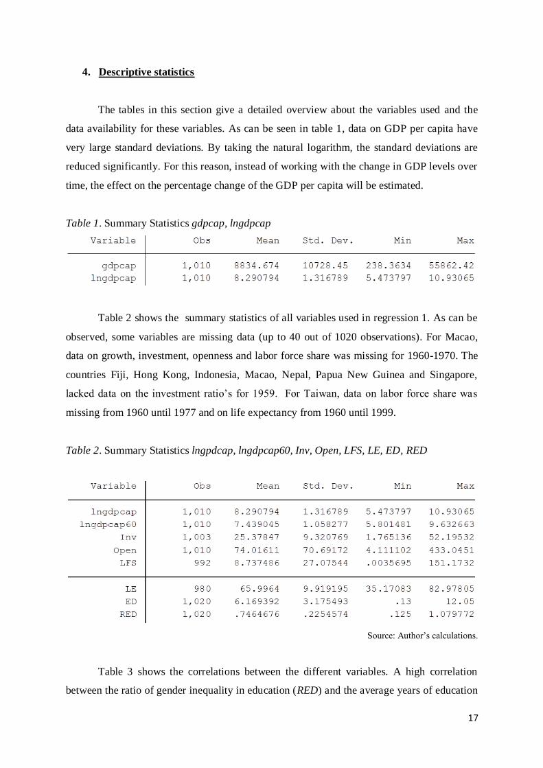
The tables in this section give a detailed overview about the variables used and the
data availability for these variables. As can be seen in table 1, data on GDP per capita have
very large standard deviations. By taking the natural logarithm, the standard deviations are
reduced significantly. For this reason, instead of working with the change in GDP levels over
time, the effect on the percentage change of the GDP per capita will be estimated.
Table 1. Summary Statistics gdpcap, lngdpcap
Table 2 shows the summary statistics of all variables used in regression 1. As can be
observed, some variables are missing data (up to 40 out of 1020 observations). For Macao,
data on growth, investment, openness and labor force share was missing for 1960-1970. The
countries Fiji, Hong Kong, Indonesia, Macao, Nepal, Papua New Guinea and Singapore,
lacked data on the investment ratio’s for 1959. For Taiwan, data on labor force share was
missing from 1960 until 1977 and on life expectancy from 1960 until 1999.
Table 2. Summary Statistics lngpdcap, lngdpcap60, Inv, Open, LFS, LE, ED, RED
Source: Author’s calculations.
Table 3 shows the correlations between the different variables. A high correlation
between the ratio of gender inequality in education (RED) and the average years of education
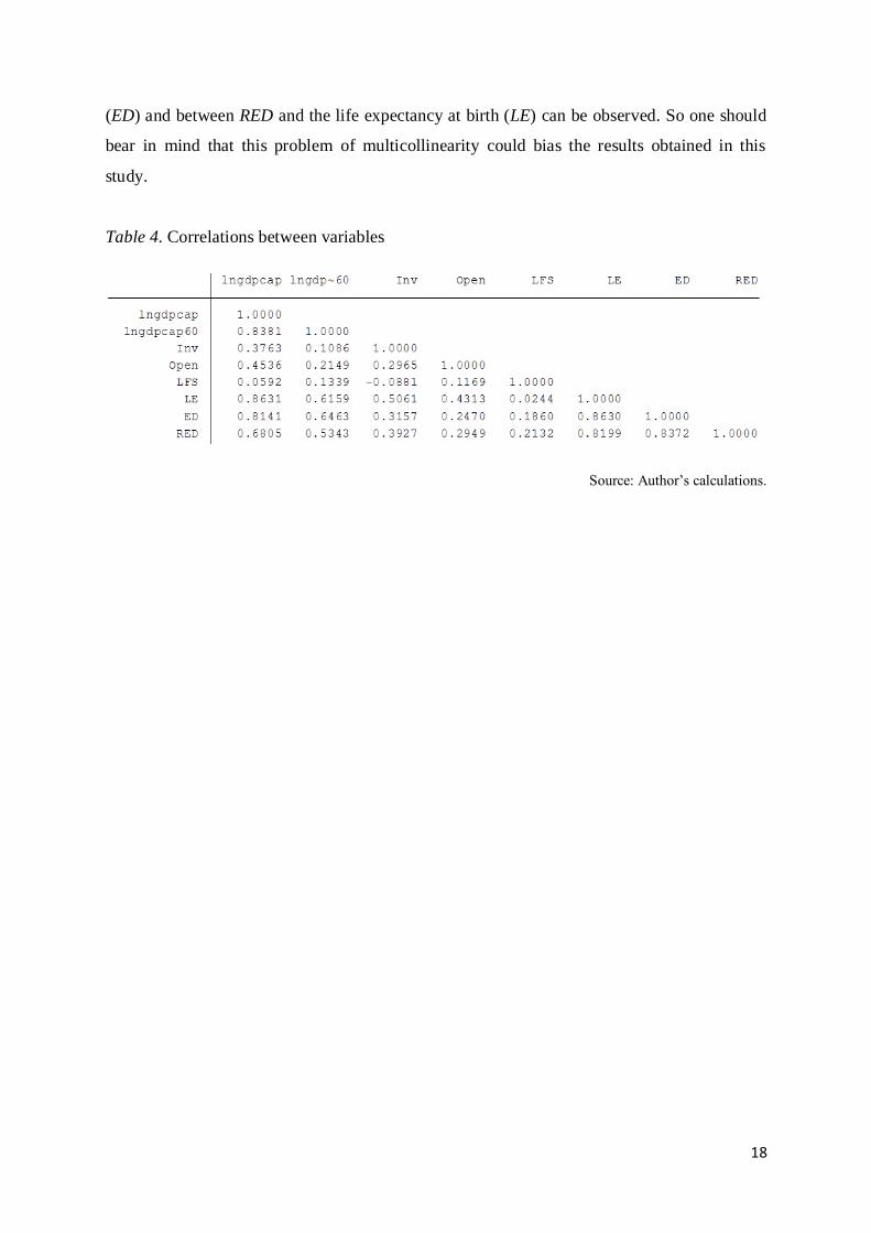
18
(ED) and between RED and the life expectancy at birth (LE) can be observed. So one should
bear in mind that this problem of multicollinearity could bias the results obtained in this
study.
Table 4. Correlations between variables
Source: Author’s calculations.
19
5. Empirical results and analysis
5.1 Results for the basic model
This section will present the results for both the direct and indirect effects that the
gender inequality in education has on the economic growth based on regression 1.1, 2, 3, and
4. Further this section the overall effect will be computed. Appendix 3 and 4 display the
results of the panel regressions. The dummy variables will be included in section 5.2 to check
the robustness of the results of the basic model. Because the natural logarithm of GDP per
capita is taken as the dependent variable in regression 1.1, the coefficients should be
interpreted by the following way: a unit change in the independent variable z will change the
GDP per capita with 𝛽𝑧%. So an increase of 1 in the average annual rate of investment as a
percentage of GDP would increase the GDP per capita with 0.00964 percentage points.
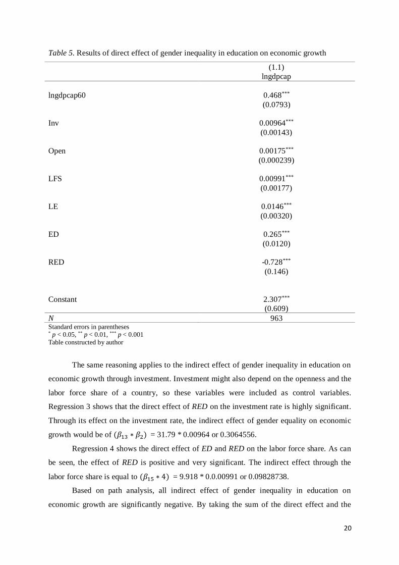
The results of regression 1.1 are presented in table 5. As can be observed, most
control variables have a significant positive impact on the GDP per capita. These results are
consistent with the expectations discussed before and confirm the findings of previous
studies. The outcome for the conditional convergence variable however is contradicting with
previous studies and with the Solow Growth Model. For the countries from South-East Asia
and the Pacific, it appears that low initial levels of GDP per capita lead to lower future
economic growth.
Also our variable of interest RED is inconsistent with our expectations since it has a
negative direct effect on GDP per capita with a p-value smaller than 0.001. The model
predicts an increase of 1 in the female-male ratio of average total years of schooling of the
adult population to lead to a decrease of 0.728 percentage points in the GDP per capita. This
implies that gender inequality has a direct positive effect on economic growth.
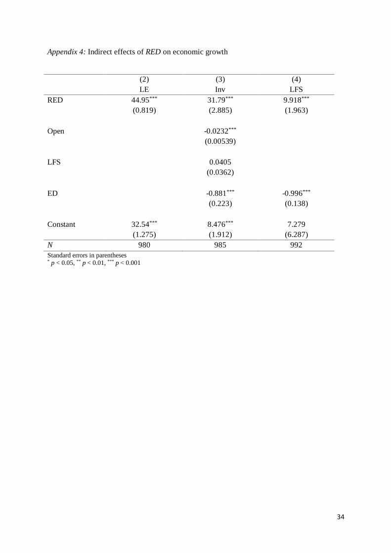
Regressions 2 until 4 in Appendix 4 explain the indirect effects of gender inequality in
education on economic growth. Regression 2 regresses RED on the average life expectancy at
birth, LE. The variable RED seems to have a very significant positive effect on the life
expectancy. Life expectancy on its turn positively affects the GDP per capita. Based on path
analysis, this finding leads to an indirect positive effect of RED on GDP per capita of (𝛽9 ∗
𝛽5) = 44.95 * 0.0146 or 0.65627. This implies a negative indirect effect of gender inequality
in education on economic growth.
20
Table 5. Results of direct effect of gender inequality in education on economic growth
(1.1)
lngdpcap
lngdpcap60 0.468***
(0.0793)
Inv 0.00964***
(0.00143)
Open 0.00175***
(0.000239)
LFS 0.00991***
(0.00177)
LE 0.0146***
(0.00320)
ED 0.265***
(0.0120)
RED -0.728***
(0.146)
Constant 2.307***
(0.609)
N 963 Standard errors in parentheses * p < 0.05, ** p < 0.01, *** p < 0.001
Table constructed by author
The same reasoning applies to the indirect effect of gender inequality in education on
economic growth through investment. Investment might also depend on the openness and the
labor force share of a country, so these variables were included as control variables.
Regression 3 shows that the direct effect of RED on the investment rate is highly significant.
Through its effect on the investment rate, the indirect effect of gender equality on economic
growth would be of (𝛽13 ∗ 𝛽2) = 31.79 * 0.00964 or 0.3064556.
Regression 4 shows the direct effect of ED and RED on the labor force share. As can
be seen, the effect of RED is positive and very significant. The indirect effect through the
labor force share is equal to (𝛽15 ∗ 4) = 9.918 * 0.0.00991 or 0.09828738.
Based on path analysis, all indirect effect of gender inequality in education on
economic growth are significantly negative. By taking the sum of the direct effect and the
21
indirect effect that RED has on GDP per capita, an overall effect of -0.728 + 0.65627 +
0.3064556 + 0.09828738 = 0.33301298 can be concluded. The positive indirect effect of
RED through the investment rate, the life expectancy at birth and the labor force share seems
to outweigh the negative direct effect of RED on LNGDPCAP. This indicates that 1
percentage point increase in the female-male ratio on average years of schooling, will
increase the economic growth by 0.0033 percentage points. Put differently, decreasing the
gender inequality causes the economic growth to increase.
5.2 Results for the model including time, country and region dummies
To check the robustness of the results on the positive direct effect of gender inequality
in education on economic growth in section 5.1, some dummy variables will be added or
combined to regression 1.1. The East Asian financial crisis that hit in 1997 could have a
regional negative effect on economic growth for those countries (Radelet and Sachs, 1998).
That is why the 20 countries included in the analysis have been divided into 3 different
regions: East Asia (EA), South Asia (SA) and the Pacific (PAC). The dummy is constructed in
the following way: EA = 1 if country is situated in the region East Asia, EA = 0 otherwise; SA
= 1 if country is situated in the region South Asia, SA = 0 otherwise. So these dummy
variables explain the differences between the Pacific and the other regions.
Besides region dummies, we also look at the effect of country dummy variables. The
crisis did not hit every country equally hard, so it could be that country dummies will lead to
more significant results than the regional dummy variables. They explain the differences
between Australia and the other countries.
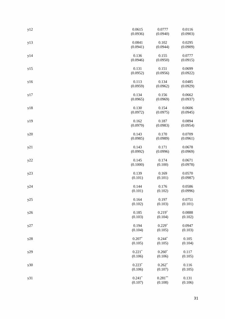
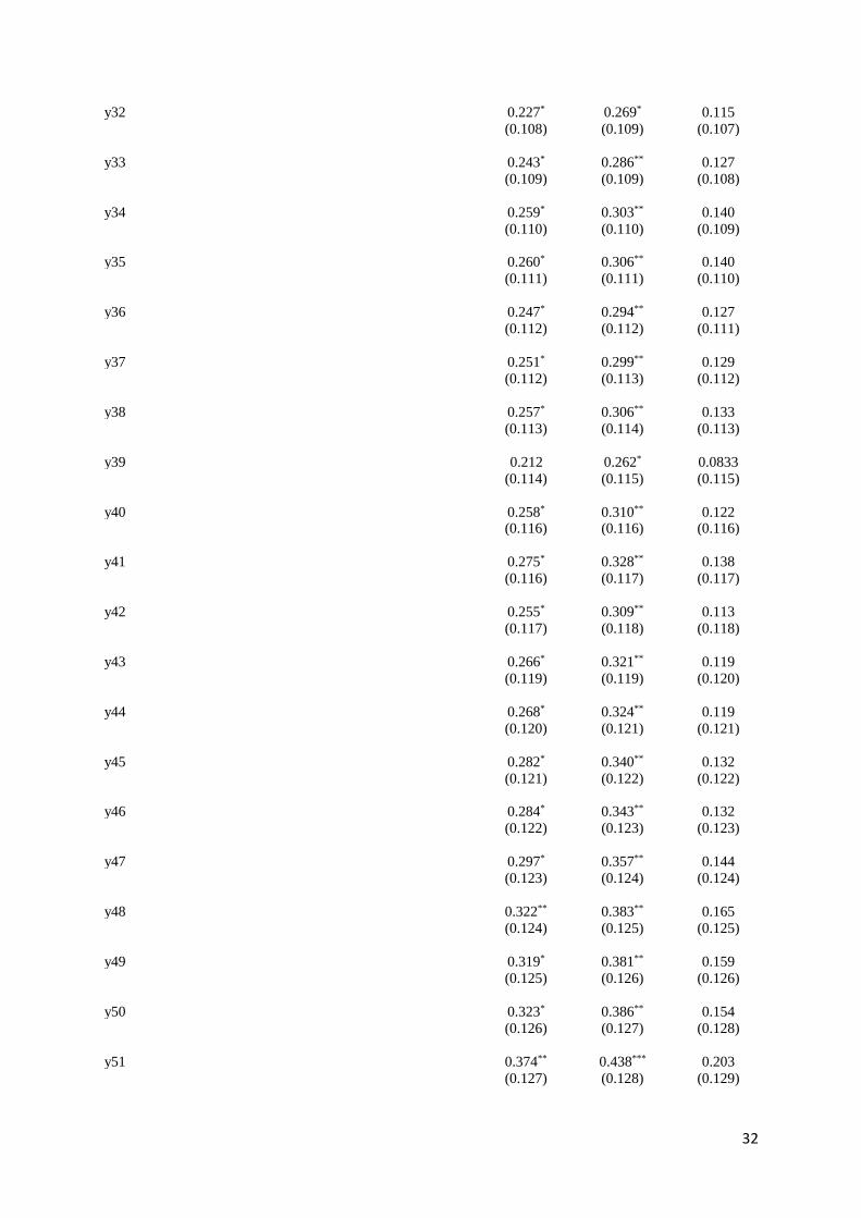
Also yearly dummy variables will be taken into account because they also could
potentially explain fluctuations in the economic growth due to the East Asian financial crisis
and so lead to more accurate estimates for our variable of interest RED. The yearly dummy
variables will explain the differences between the year 1960 and the other years. Data ranges
from 1960 until 2010. The year 1960 is represented by y1, year 1961 by y2, year 1962 by y3
etc. until year 2010 is represented by y51.
These variables will be regressed individually and combined. The results can be found
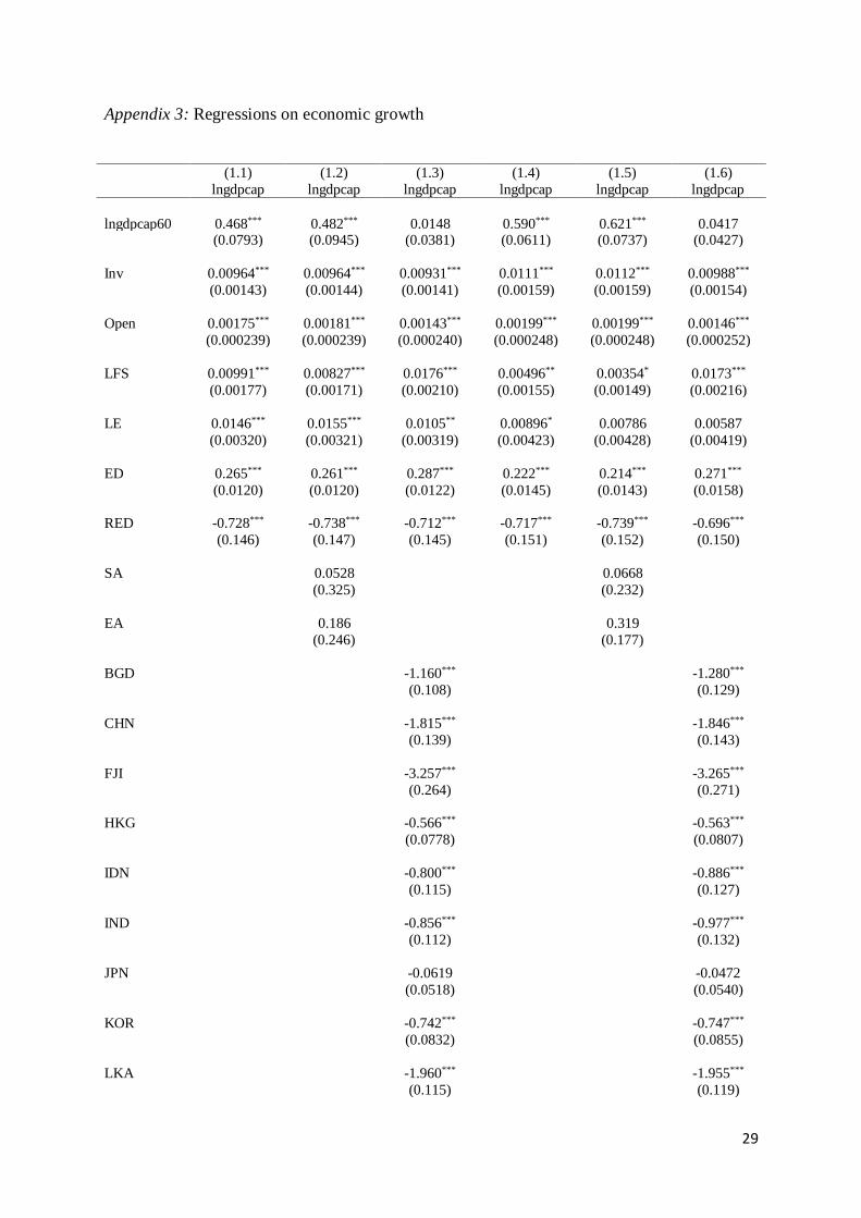
in Appendix 3 in the regressions 1.2-1.6. In regression 1.2 regional dummy variables are
added to regression 1.1, country dummies in regression 1.3, year dummies in regression 1.4,
region and year dummies combined in regression 1.5 and country and year dummies in
regression 1.6.
22
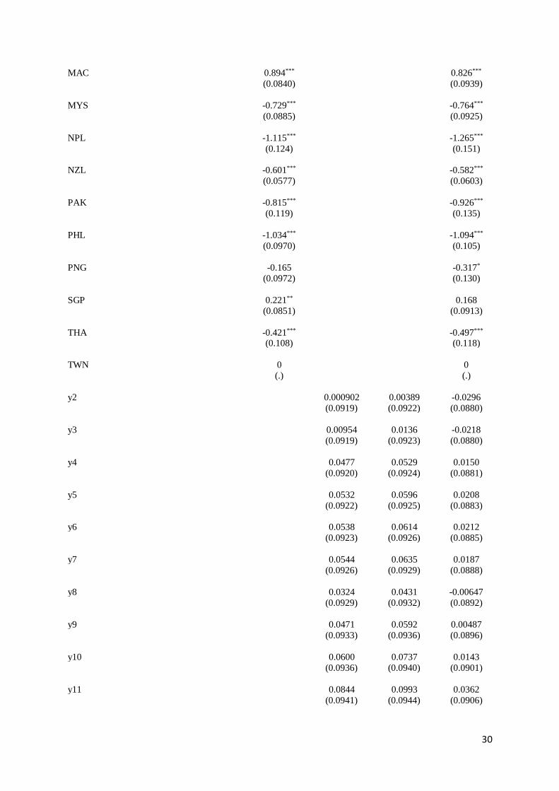
As can be observed in Appendix 3, the country dummy variables have a highly
significant effect on the economic growth whereas the region and yearly dummy variables
contain very little significance. More important is to note that in all regressions, the gender
inequality in education ratio has a very high significance with coefficients ranging from
-0.739 to -0.696. We can conclude that the results about the negative direct effect of RED on
LNGDPCAP of -0.728 from regression 1.1 in section 5 is robust.
23
6. Conclusion
Gender inequality in education is an issue that should be addressed in order to
increase the overall well-being of women. This paper tried to give additional motives on why
gender inequality should be reduced by finding out whether reducing inequality has a positive
on the economic growth for countries in South-East Asia and the Pacific. If so, politicians
would have additional incentives to increase schooling for girls in the Middle East, Central
Asia and Africa since enrollment ratios in these regions are still very gender biased.
Based on the significant increase in gender equality in education along with proper
growth rates in South-East Asia and the Pacific, the study will focus on 20 countries from
these regions. This research is based on yearly panel data between 1960 and 2010 and finds a
positive direct effect of gender inequality in education on economic development and a
negative indirect effect through the investment rate, the life expectancy at birth and the labor
force share. By taking the sum of both effects, an overall effect of 0.333 has been conducted.
This means that for countries in South-East Asia and the Pacific, increasing the gender
inequality ratio in education by 1 percentage point will lead to an increase of GDP per capita
by 0.003 percentage point.
The results of the total effect of gender inequality in education slowing down
economic growth in this paper is in line with the results of previous studies on similar topics.
Klasen (2002), Klasen and Lamanna (2009), Dollar & Gatti (2001) and Knowles et al. (2002)
also found a negative effect of gender inequality in education on economic growth. However,
where this paper found a positive direct effect, some studies (Klasen, 2002; Klasen and
Lamanna, 2009) found a negative direct effect. These differences in results could be due to
our sample being limited to countries in South-East Asia and the Pacific compared to
worldwide cross-country selection by other studies. Seguino (2000) also limited her study but
to a set of semi-industrialized (mostly Asian) countries and implied a positive effect of
gender inequality in education on economic growth. Seguino (2000) however also concluded
that gender inequality stimulates investment, where our paper concludes the opposite.
We can conclude that one should properly reflect on the methodologies and the
sample selection of the studies done so far on this topic. There is a clear difference in results
based on a variety of countries worldwide and results based on only a subset of countries. A
proper study on why these results are significantly different should be conducted.
Recommendations for further research would be to study the indirect effect of gender
inequality on economic growth through the labor force participation rate. Due to a lack of
24
data, this was not performed in this paper. Researching this issue would be interesting to see
whether higher education levels for girls will be translated in to a higher participation rate of
women in society. This on its turn could have a significant effect on the growth of a country.
Also similar research with a sample that includes different subsets of countries would be
recommended to check whether that leads to similar results compared to previous studies on a
wide variety of countries worldwide. Also one could update this paper using the lagged
values for openness and RED to limit simultaneous causality problems.
Results suggest that one should continue promoting gender equality in education.
Especially in Africa, the Middle East and Central Asia where gender inequality in education
still persists. Besides being incentivized solely to boost economic growth, one should have
more incentives to reduce gender inequality in education for the sake of women’s well-being
and for the other consequences of more gender equality in education such as its positive
impact on health, child education and mortality rates.
25
References
Aliber, M. (2003). Chronic Poverty in South Africa: Incidence, Causes and Policies. World
Development, 31(3), 473-490. doi: 10.1016/S0305-750X(02)00219-X
Barro, R. (2001). Human Capital: Growth, History, and Policy. American Economic
Association, 91(2), 12-17.
Barro, R. J., & Lee, J. W. (1994, June). Sources of economic growth. In Carnegie-Rochester
conference series on public policy (Vol. 40, pp. 1-46). North-Holland.
Cooray, A. & Potrafke, N. (2011). Gender inequality in education: Political institutions or
culture and religion? European Journal op Political Economy, 27(1), 268-280.
doi:10.1016/j.ejpoleco.2010.08.004
Duflo, E. (2012). Women Empowerment and Economic Development. Journal of Economic
Literature, 50(4), 1051–1079. doi: 10.1257/jel.50.4.1051
Dollar, D. & Gatti, R. (1999). Gender Inquality, Income, and Growth: Are Good Times Good
for Women? World Bank Working Paper
Hicks, D. (1997). The Inequality-Adjusted Human Development Index: A Constructive
Proposal. World Development, 25(8), 1283-1298.
Jacobs, J. (1996). Gender Inequality and Higher Education. Annual Reviews Sociology, 22(1),
pp. 153-185.
Kabeer, N. (2005). Gender Equality and Women's Empowerment: A Critical Analysis of the
Third Millennium Development Goal. Gender and Development, 13(1), 13-24.
Klasen, S. (2002). Low Schooling for Girls, Slower Growth for All? Cross-Country Evidence
on the Effect of Gender Inequality in Education on Economic Development. The
World Bank Economic Review, 16(3), 345-373.
doi:2048/10.1080/13545700902893106
26
Klasen, S., Lamanna, F. (2009). The Impact of Gender Inequality in Education and
Employment on Economic Growth: New Evidence for a Panel of Countries. Feminist
Economics, 15(3), 91-132. doi: 10.1080/13545700902893106
Knowles, S., Lorgelly, P. & Owen, P. (2002). Are educational gender gaps a brake on
economic development? Some cross-country empirical evidence. Oxford Economic
Papers, 54 (1), 118-149.
Krugman, P.R. , Obstfeld, M. and Melitz, M.J. (2015), International Economics. Theory &
Policy, 10th edition, Pearson Global Edition, ISBN-10: 1-292-01955-7, ISBN-13:
978-1-292-01955-0, Chapters 1-12.
Radelet, S., & Sachs, J. (1998). The onset of the East Asian financial crisis (No. w6680).
National bureau of economic research. Romer, D. (2011), Advanced Macroeconomics, fourth
edition, McGraw-Hill, New York.
Seguino, S. (2000). Gender Inequality and Economic Growth: A Cross-Country Analysis.
World Development, 28 (7), 1211-1230.
Sen, A. (1990). More Than 100 Million Women Are Missing. The New York Review of
Books, 37(20)
Stotsky, J., Shibuya, S., Kolovich, L. and Kebhaj, S. (2016). Trends in Gender Equality and
Women’s Advancement. IMF Working Paper
United Nations (2015). The Millennium Development Goals Report 2015.
Unterhalter, E. (2006). Measuring Gender Inequality in Education in South Asia. United
Nations Children’s Fund
27
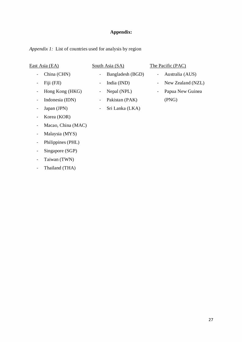
Appendix:
Appendix 1: List of countries used for analysis by region
East Asia (EA) South Asia (SA) The Pacific (PAC)
- China (CHN)
- Fiji (FJI)
- Hong Kong (HKG)
- Indonesia (IDN)
- Japan (JPN)
- Korea (KOR)
- Macao, China (MAC)
- Malaysia (MYS)
- Philippines (PHL)
- Singapore (SGP)
- Taiwan (TWN)
- Thailand (THA)
- Bangladesh (BGD)
- India (IND)
- Nepal (NPL)
- Pakistan (PAK)
- Sri Lanka (LKA)
- Australia (AUS)
- New Zealand (NZL)
- Papua New Guinea
(PNG)
28
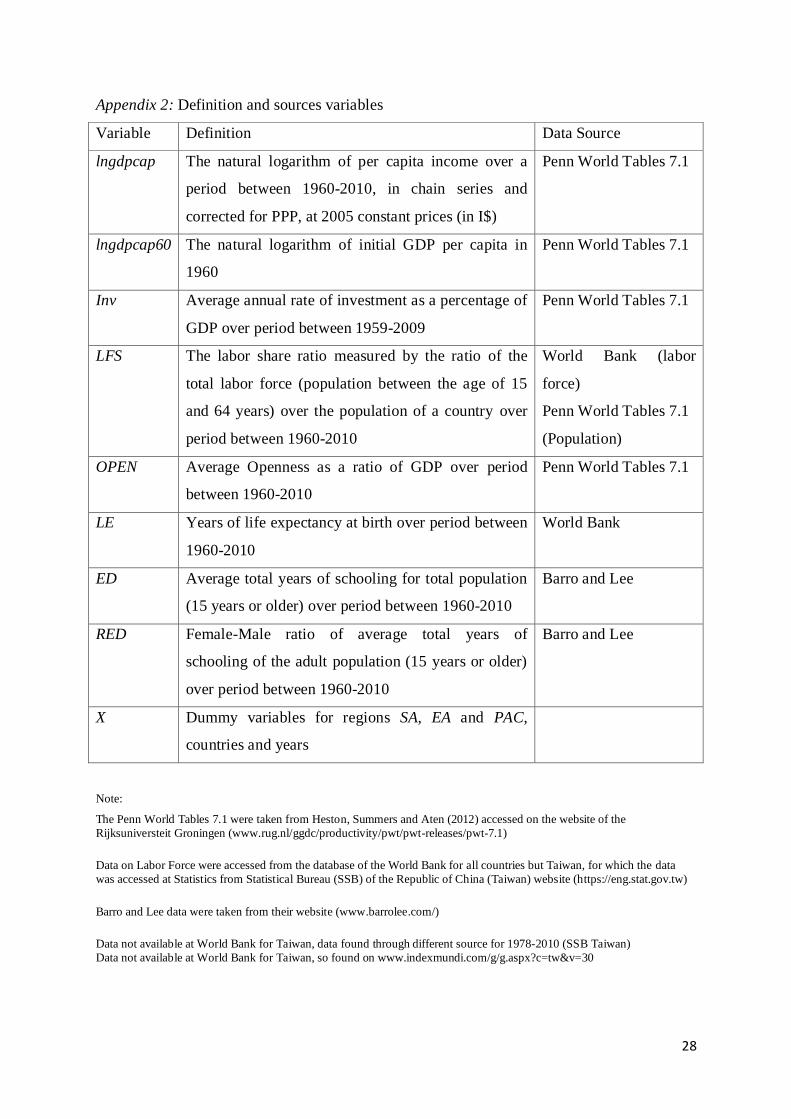
Appendix 2: Definition and sources variables
Variable Definition Data Source
lngdpcap The natural logarithm of per capita income over a
period between 1960-2010, in chain series and
corrected for PPP, at 2005 constant prices (in I$)
Penn World Tables 7.1
lngdpcap60 The natural logarithm of initial GDP per capita in
1960
Penn World Tables 7.1
Inv Average annual rate of investment as a percentage of
GDP over period between 1959-2009
Penn World Tables 7.1
LFS The labor share ratio measured by the ratio of the
total labor force (population between the age of 15
and 64 years) over the population of a country over
period between 1960-2010
World Bank (labor
force)
Penn World Tables 7.1
(Population)
OPEN Average Openness as a ratio of GDP over period
between 1960-2010
Penn World Tables 7.1
LE Years of life expectancy at birth over period between
1960-2010
World Bank
ED Average total years of schooling for total population
(15 years or older) over period between 1960-2010
Barro and Lee
RED Female-Male ratio of average total years of
schooling of the adult population (15 years or older)
over period between 1960-2010
Barro and Lee
X Dummy variables for regions SA, EA and PAC,
countries and years
Note:
The Penn World Tables 7.1 were taken from Heston, Summers and Aten (2012) accessed on the website of the
Rijksuniversteit Groningen (www.rug.nl/ggdc/productivity/pwt/pwt-releases/pwt-7.1)
Data on Labor Force were accessed from the database of the World Bank for all countries but Taiwan, for which the data
was accessed at Statistics from Statistical Bureau (SSB) of the Republic of China (Taiwan) website (https://eng.stat.gov.tw)
Barro and Lee data were taken from their website (www.barrolee.com/)
Data not available at World Bank for Taiwan, data found through different source for 1978-2010 (SSB Taiwan)
Data not available at World Bank for Taiwan, so found on www.indexmundi.com/g/g.aspx?c=tw&v=30
29
Appendix 3: Regressions on economic growth
(1.1) (1.2) (1.3) (1.4) (1.5) (1.6)
lngdpcap lngdpcap lngdpcap lngdpcap lngdpcap lngdpcap
lngdpcap60 0.468*** 0.482*** 0.0148 0.590*** 0.621*** 0.0417 (0.0793) (0.0945) (0.0381) (0.0611) (0.0737) (0.0427)
Inv 0.00964*** 0.00964*** 0.00931*** 0.0111*** 0.0112*** 0.00988***
(0.00143) (0.00144) (0.00141) (0.00159) (0.00159) (0.00154)
Open 0.00175*** 0.00181*** 0.00143*** 0.00199*** 0.00199*** 0.00146***
(0.000239) (0.000239) (0.000240) (0.000248) (0.000248) (0.000252)
LFS 0.00991*** 0.00827*** 0.0176*** 0.00496** 0.00354* 0.0173***
(0.00177) (0.00171) (0.00210) (0.00155) (0.00149) (0.00216)
LE 0.0146*** 0.0155*** 0.0105** 0.00896* 0.00786 0.00587
(0.00320) (0.00321) (0.00319) (0.00423) (0.00428) (0.00419)
ED 0.265*** 0.261*** 0.287*** 0.222*** 0.214*** 0.271***
(0.0120) (0.0120) (0.0122) (0.0145) (0.0143) (0.0158)
RED -0.728*** -0.738*** -0.712*** -0.717*** -0.739*** -0.696***
(0.146) (0.147) (0.145) (0.151) (0.152) (0.150)
SA 0.0528 0.0668
(0.325) (0.232)
EA 0.186 0.319
(0.246) (0.177)
BGD -1.160*** -1.280***
(0.108) (0.129)
CHN -1.815*** -1.846***
(0.139) (0.143)
FJI -3.257*** -3.265***
(0.264) (0.271)
HKG -0.566*** -0.563***
(0.0778) (0.0807)
IDN -0.800*** -0.886***
(0.115) (0.127)
IND -0.856*** -0.977***
(0.112) (0.132)
JPN -0.0619 -0.0472
(0.0518) (0.0540)
KOR -0.742*** -0.747***
(0.0832) (0.0855)
LKA -1.960*** -1.955***
(0.115) (0.119)
30
MAC 0.894*** 0.826***
(0.0840) (0.0939)
MYS -0.729*** -0.764***
(0.0885) (0.0925)
NPL -1.115*** -1.265***
(0.124) (0.151)
NZL -0.601*** -0.582***
(0.0577) (0.0603)
PAK -0.815*** -0.926***
(0.119) (0.135)
PHL -1.034*** -1.094***
(0.0970) (0.105)
PNG -0.165 -0.317*
(0.0972) (0.130)
SGP 0.221** 0.168
(0.0851) (0.0913)
THA -0.421*** -0.497*** (0.108) (0.118)
TWN 0 0
(.) (.)
y2 0.000902 0.00389 -0.0296
(0.0919) (0.0922) (0.0880)
y3 0.00954 0.0136 -0.0218
(0.0919) (0.0923) (0.0880)
y4 0.0477 0.0529 0.0150
(0.0920) (0.0924) (0.0881)
y5 0.0532 0.0596 0.0208
(0.0922) (0.0925) (0.0883)
y6 0.0538 0.0614 0.0212
(0.0923) (0.0926) (0.0885)
y7 0.0544 0.0635 0.0187
(0.0926) (0.0929) (0.0888)
y8 0.0324 0.0431 -0.00647
(0.0929) (0.0932) (0.0892)
y9 0.0471 0.0592 0.00487
(0.0933) (0.0936) (0.0896)
y10 0.0600 0.0737 0.0143
(0.0936) (0.0940) (0.0901)
y11 0.0844 0.0993 0.0362
(0.0941) (0.0944) (0.0906)
31
y12 0.0615 0.0777 0.0116
(0.0936) (0.0940) (0.0903)
y13 0.0841 0.102 0.0295
(0.0941) (0.0944) (0.0909)
y14 0.136 0.155 0.0777
(0.0946) (0.0950) (0.0915)
y15 0.131 0.151 0.0699
(0.0952) (0.0956) (0.0922)
y16 0.113 0.134 0.0485
(0.0959) (0.0962) (0.0929)
y17 0.134 0.156 0.0662
(0.0965) (0.0969) (0.0937)
y18 0.130 0.154 0.0606
(0.0972) (0.0975) (0.0945)
y19 0.162 0.187 0.0894
(0.0979) (0.0983) (0.0954)
y20 0.143 0.170 0.0709 (0.0985) (0.0989) (0.0961)
y21 0.143 0.171 0.0678
(0.0992) (0.0996) (0.0969)
y22 0.145 0.174 0.0671
(0.1000) (0.100) (0.0978)
y23 0.139 0.169 0.0570
(0.101) (0.101) (0.0987)
y24 0.144 0.176 0.0586
(0.101) (0.102) (0.0996)
y25 0.164 0.197 0.0751
(0.102) (0.103) (0.101)
y26 0.185 0.219* 0.0888
(0.103) (0.104) (0.102)
y27 0.194 0.229* 0.0947
(0.104) (0.105) (0.103)
y28 0.207* 0.244* 0.105
(0.105) (0.105) (0.104)
y29 0.221* 0.260* 0.117
(0.106) (0.106) (0.105)
y30 0.223* 0.262* 0.116
(0.106) (0.107) (0.105)
y31 0.241* 0.281** 0.131
(0.107) (0.108) (0.106)
32
y32 0.227* 0.269* 0.115
(0.108) (0.109) (0.107)
y33 0.243* 0.286** 0.127
(0.109) (0.109) (0.108)
y34 0.259* 0.303** 0.140
(0.110) (0.110) (0.109)
y35 0.260* 0.306** 0.140
(0.111) (0.111) (0.110)
y36 0.247* 0.294** 0.127
(0.112) (0.112) (0.111)
y37 0.251* 0.299** 0.129
(0.112) (0.113) (0.112)
y38 0.257* 0.306** 0.133
(0.113) (0.114) (0.113)
y39 0.212 0.262* 0.0833
(0.114) (0.115) (0.115)
y40 0.258* 0.310** 0.122 (0.116) (0.116) (0.116)
y41 0.275* 0.328** 0.138
(0.116) (0.117) (0.117)
y42 0.255* 0.309** 0.113
(0.117) (0.118) (0.118)
y43 0.266* 0.321** 0.119
(0.119) (0.119) (0.120)
y44 0.268* 0.324** 0.119
(0.120) (0.121) (0.121)
y45 0.282* 0.340** 0.132
(0.121) (0.122) (0.122)
y46 0.284* 0.343** 0.132
(0.122) (0.123) (0.123)
y47 0.297* 0.357** 0.144
(0.123) (0.124) (0.124)
y48 0.322** 0.383** 0.165
(0.124) (0.125) (0.125)
y49 0.319* 0.381** 0.159
(0.125) (0.126) (0.126)
y50 0.323* 0.386** 0.154
(0.126) (0.127) (0.128)
y51 0.374** 0.438*** 0.203
(0.127) (0.128) (0.129)
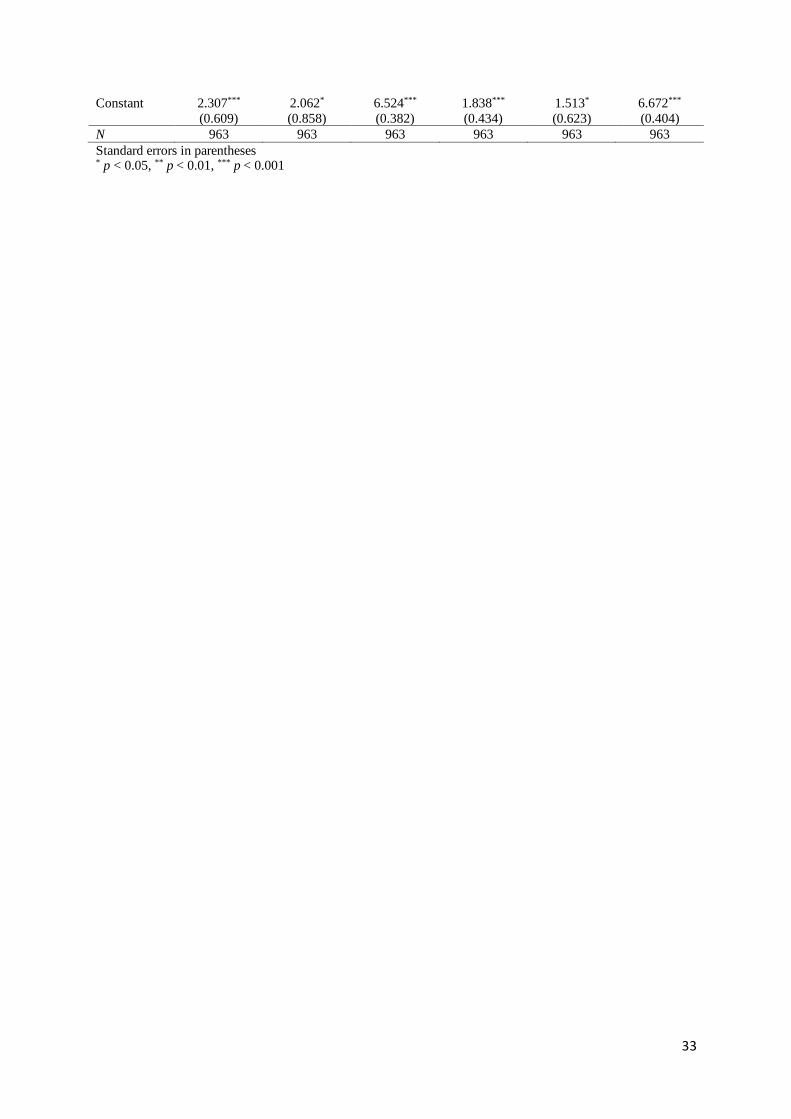
33
Constant 2.307*** 2.062* 6.524*** 1.838*** 1.513* 6.672***
(0.609) (0.858) (0.382) (0.434) (0.623) (0.404)
N 963 963 963 963 963 963
Standard errors in parentheses * p < 0.05, ** p < 0.01, *** p < 0.001
34
Appendix 4: Indirect effects of RED on economic growth
(2) (3) (4)
LE Inv LFS
RED 44.95*** 31.79*** 9.918***
(0.819) (2.885) (1.963)
Open -0.0232***
(0.00539)
LFS 0.0405
(0.0362)
ED -0.881*** -0.996***
(0.223) (0.138)
Constant 32.54*** 8.476*** 7.279
(1.275) (1.912) (6.287)
N 980 985 992
Standard errors in parentheses * p < 0.05, ** p < 0.01, *** p < 0.001