THE UNIVERSITY OF KWAZULU-NATAL

THE EFFECT OF FRETTING MARKS INTRODUCED

DURING STRAND WINDING ON THE FATIGUE

PERFORMANCE OF TRANSMISSION LINE

CONDUCTORS

Larry Chama Botha

213570453

Supervisors:

Dr Richard Loubser

Dr Rob Stephen

Dr Innocent Davidson

December, 2015

Submitted in fulfilment of the academic requirements for the degree of Master of Science in Engineering at the School of Mechanical Engineering, University of KwaZulu-Natal

i | P a g e

DECLARATION 1-PLAGIARISM

I, Larry Chama Botha, declare that

1. The research report in this thesis, except where otherwise indicated, is my own original

research.

2. This thesis is not submitted for any degree or examination at any other university.

3. This thesis does not contain other persons’ data, pictures graphs or other information,

unless specifically acknowledged as being sourced from other persons

4. This thesis does not contain other persons’ writing, unless specifically acknowledged as

being sourced from other researchers. Where other written sources have been quoted, then:

a) Their work has been re-written but general but general information attributed to them

as been referenced

b) Where their exact words have been used, then their writing has been placed in italics

and inside quotation marks, and referenced.

5. This thesis does not contain text, graphics or tables copied and pasted from the internet,

unless specifically acknowledged, and the source being detailed in the thesis and in the

Reference sections.

Signed

……………………………………………………………………………………………………

SUPERVISOR

As the candidate’s Supervisor I agree/do not agree to the submission of this thesis

Signed

……………………………………………………………………………………………………

ii | P a g e

DECLARATION 2-PUBLICATIONS

DETAILS OF CONTRIBUTION TO PUBLICATIONS

1. Elasto-Plastic Interlayer contact modelling of the Tern Conductor, The Journal of

Strain Analysis for Engineering Design

2. The Effect of Fretting Marks Introduced During Strand Winding on the Fatigue

Performance of Transmission Line Conductors, IEE-PES Conference, 2016

3. Improving the Quality of Overhead Line Conductors during Manufacturing,

IEEE- PES Conference, 2016

Signed:

…………………………………………………………………………………………………………………………………………………

iii | P a g e

Abstract

In this research, the Elasto-plastic interlayer contact of the TERN ACSR conductor used on

Eskom’s 400kV transmission lines is investigated. Characterization of the elliptical contact

marks using eucentric tilting in SEM stereomicroscopy for depth measurement is conducted.

The size of these manufacturing defects (fret marks) resulting from the strand winding process

is quantified.

The already established observation that two geometrically dissimilar contacting surfaces may

exhibit the same contact mechanics is extensively used to explain how the variations in

stranding lay ratios affects the size of the fret marks and hence the surface quality of strands.

From this supposition, an equivalent contacting sphere radius is calculated and used for both

nonlinear and linear elastic finite element Analysis (FEA) in MSC Marc mentat.

An inner conductor contact mechanics model for determining the normal contact force per

defect is also presented and used with existing inner conductor mechanics models for tension

determination. The calculated equivalent radius shows strong linear correlation with the defect

size, contact force, plastic strain and stress and can therefore be used in the design of

conductors.

Fatigue testing was then conducted on two (02) TERN conductors. Fractographic analysis of

the samples exposed to fatigue cycles was conducted using the Scanning Electron Microscopy

(SEM) and Field Emission SEM (FEGSEM). Energy Dispersive Spectroscopy was also used

for Surface Elemental analysis before and after the fatigue testing to analyse the changes in

material composition on the fret mark surfaces.

iv

Acknowledgements

I would like to thank;

1. My core Supervisors Dr Richard Loubser and Dr Rob Stephen for their invaluable

technical input and guidance throughout the course of my research

2. Mr Pravesh Moodley for is assistance in the setting up of the fatigue tests and during the

fatigue testing

3. Mr Bertie Jacobs of Eskom for his input from the inception of this research

4. My family and friends for their patience, understanding and motivation

5. Aberdare Cables, South Africa for their financial support, technical input and provision of

conductor samples

6. THRIP and the University of KwaZulu-Natal for their financial support

7. The Microscopy and Microanalysis Unit (MMU) of the University of KwaZulu-Natal for

their dedication and patience

8. Eskom holdings for the infrastructure support and the training offered via Trans Africa

Projects (TAP)

9. Dr Innocent Davidson for the administrative support, encouragement and guidance

10. Mr Henni Scholtz and Mr Jonathan Young of Aberdare cables for the provision of the

necessary standards and controlled documents needed for this research.

v

List of Acronyms

ACSR Aluminium Conductor Steel Reinforced

OHL Overhead Line Conductor

EDS Every Day Stress

EDS(X) Electron Dispersive Spectroscopy

SEM Scanning Electron Microscope

FEGSEM Field Emission Gun Scanning Electron Microscope

LVDT Linear Voltage Differential Transform

FCC Fatigue crack propagation

LE Linear Elastic

FEA Finite Element Analysis

SANS South Africa National Standards

IEC International Electrotechnical Commission

EIFS Initial Equivalent Flaw Size

IFS Initial Flaw Size

vi | P a g e

List of Symbols

D0 Outer diameter of conductor

ns Number of still wires

ds Diameter of the steel wires

da Diameter of aluminium wire

na Number of aluminium wires

no Number of wires in the outer layer

Re Reynolds number

D Diameter of the Conductor

V Wind speed

v Viscosity coefficient

S Strouhal number

Fw Frequency of the turbulences

A Projected area of the conductor

𝜔 Angular frequency

t Time

Rw Radius of the strand

w Width of the fret mark

f Resonant frequency

L Span Length

n Mode of the vibration

Rl Lead wire resistance

Rg Nominal strain gauge resistance

GF Gauge factor of the strain gauge

휀 Strain (in micro-strains)

V0 Bridge output voltage

V0 (Unstrained) Bridge output voltage

Vex Excitation voltage

D Mean diameter or pitch

P Lay length

Yb Bending amplitude

E Modulus of Elastic

𝜎𝑏 Bending stress ( 0 to peak)

d Diameter of the outer strand

T Conductor tension

vii | P a g e

E*I Flexural rigidity F Force

K Stiffness

X Displacement

Ac Cross section area and the

Ec Young Modulus of the core

∆𝐾 Stress intensity factor range

Smin , Smax Maximum and Minimum Stresses in the cycle

a Crack length

∆𝜎 Stress range

D Diameter of the strand

M Moment

I Second moment of area

𝜎 Stress

γ Lay ratio

∆𝐾𝑐 Fracture toughness

viii

Table of Contents

Contents DECLARATION 1-PLAGIARISM ..........................................................................................

DECLARATION 2-PUBLICATIONS .................................................................................... ii

Abstract ..................................................................................................................................... iii

1. Introduction ........................................................................................................................... 4

1.1 Aluminium Conductor Steel Reinforced (ACSR) ....................................................... 6

1.2 Manufacturing Process of ACSR Conductors ............................................................. 7

1.2.1 Rotation of tubular body ..................................................................................... 8

1.2.2 Feed motion ....................................................................................................... 10

1.2.3 Greasing of Conductors..................................................................................... 12

1.3 Aeolian Vibrations on Overhead Transmission lines ................................................ 13

1.4 Problem statement ..................................................................................................... 16

1.5 Objectives.................................................................................................................. 17

1.6 Project justification ................................................................................................... 18

2. Fretting Fatigue ............................................................................................................... 19

2.1 Mechanism of Fretting Fatigue ...................................................................................... 19

3. Research Methodology ................................................................................................... 22

3.1 Characterization of fret marks ......................................................................................... 22

3.1.1 Sampling and surface preparation ............................................................................ 22

3.1.2 Sample preparatio .................................................................................................... 22

3.2 Stereomicroscopy ............................................................................................................ 23

3.3 Scanning electron microscopy and SEM stereomicroscopy ........................................... 26

3.4 Energy dispersive spectroscopy ................................................................................ 30

3.4.1 Sample preparation............................................................................................ 30

3.5 Tensile testing ........................................................................................................... 32

3.6 Fatigue testing ........................................................................................................... 32

3.6.1 Conductor Sample preparation .......................................................................... 37

3.6.2 Bending amplitude measurement ...................................................................... 38

3.6.3 Strain measurement ........................................................................................... 38

ix | P a g e

3.6.4 Strand breakage detection mechanism .............................................................. 41

3.6.5 Frequency sweep ............................................................................................... 43

3.6.6 Fatigue testing ................................................................................................... 43

3.7 Fractography ............................................................................................................. 45

3.7.1 Stereomicroscopy .............................................................................................. 45

3.7.2 Scanning Electron Microscopy ......................................................................... 46

3.7.3 Energy Dispersive microscopy ......................................................................... 46

4. Data Collection, Collation and Analysis ........................................................................ 47

4.1 Stereomicroscopy and scanning electron microscopy .................................................... 47

4.2 Fatigue testing results ...................................................................................................... 52

4.3 Energy dispersive spectroscopy ...................................................................................... 54

4.4 Fractography ............................................................................................................. 56

4.4.1 Nucleation and propagation of cracks ............................................................... 56

4.5 EDS on fatigue tested samples .................................................................................. 60

5. Contact Mechanics .......................................................................................................... 64

5.1 General Theory ......................................................................................................... 64

5.2 Contact modelling of the TERN conductor .............................................................. 71

5.2.1 Equation of helical curves ........................................................................................ 71

5.2.2 Strand to strand contact modelling ........................................................................... 71

5.2.3 Finite Element Analysis (FEA) ......................................................................... 76

5.2.3.2 Von Mises stress ................................................................................................... 87

5.2.3.3 Normal contact force ............................................................................................. 88

5.2.3.4 Effect of equivalent radius on the normal contact force ....................................... 88

5.2.3.5 Fret mark dimensions versus equivalent radius .................................................... 89

5.3 Inner conductor contact model .................................................................................. 91

6. Fatigue Crack Propagation ............................................................................................ 94

6.1 Crack growth and the stress intensity factor ............................................................. 94

6.2 Modelling of the fatigue data .................................................................................... 96

6.3 Equivalent Initial Flaw Size (EIFS) .......................................................................... 99

7. Conclusion...................................................................................................................... 101

8. References ...................................................................................................................... 103

Annexure A ............................................................................................................................ 105

x | P a g e

Annexure B ............................................................................................................................ 106

Annexure C ............................................................................................................................ 120

Annexure D ............................................................................................................................ 128

................................................................................................................................................. 128

1 | P a g e

List of Figures

Figure1-1: Examples of ACSR conductor………………………………………………………7

Figure1-2: Stranding Machine……………………………………………………………..........9

Figure 1-3: Position of gears A and B relative to Drive Shaft……………………………….....9

Figure 1-4: Bull wheels………………………………………………………………………..10

Figure 1-5: Power transmission line…………………………………………………………...15

Figure 1-6: Vortex shedding in cylindrical objects……………………………………………16

Figure 3-1: Specimens mounted on stub for SEM…………………………………………….23

Figure 3-2: Images from stereomicroscopy, (a) Z-staked (b) Ordinary image………………..25

Figure 3-3: Scanning Electron Microscope (SEM)……………………………………………26

Figure 3-4: 3D Stereomicroscopy……………………………………………………………..27

Figure 3-5: Fret mark depth…………………………………………………………………...28

Figure 3-6: Micrographs used in Depth Measurement………………………………………...29

Figure 3-7: EDS on fret mark surfaces………………………………….……………………..31

Figure 3-8: FEGSEM for Energy Dispersive Spectroscopy (EDS) Analysis………………...31

Figure 3-9: (a) Resonance fatigue testing bench………………………………………………36

Figure 3-9: (b) Fatigue test set-up at VRTC-UKZN…………………………………………..37

Figure 3-10: Laser Sensor at the suspension clamp for measuring bending amplitude……….38

Figure 3-11: Arrangement of strain gauges at the mouth of the clamp………………………..39

Figure 3-12: Quarter bridge configuration…………………………………………………….41

Figure 3-13: Strand breakage detection mechanism…………………………………………..42

Figure 3-14: Frequency sweep………………………………………………………………...43

Figure 3-15: LabVIEW program……………………………………………… ………….44

Figure 3-16: Indicators for Amplitude monitoring…………………………………………….48

Figure 4-1: Measuring the axes of the fret marks ……………………………………………..49

Figure 4-2: SEM 3D Stereomicroscopy……………………………………………………….46

Figure 4-3: Micrographs used for measurements……………………………………………...50

2 | P a g e

Figure 4-4: Bending Strains on the upper surface of the conductor…………………………...42

Figure 4-5 (a-d): Micrographs for fatigue tested samples……………………………………..57

Figure 4-6: Histograms for EDS analysis of results…………………………………………...62

Figure 5-1: Two dimensional bodies in mathematical contact………………………………...63

Figure 5-2: Transformation of Axes…………………………………………………………...66

Figure 5-3: Body with different orthogonal radii of curvature………………………………...67

Figure 5-4: Transformation of axes for deformation analysis…………………………………68

Figure 5-5 Global and local axes for contact analysis…………………………………………71

Figure: 5-6: Variation of the equivalent radius in the conductor samples examined………….74

Figure 5-7: (a) Large and Shallow mark for inner layer (b) Relatively Smaller and Deeper Fret mark for mid Layer……………………………………………………………………….75

Figure 5-8: 6063 Aluminium Alloy Stress-strain curve……………………………………….76

Figure 5-9: Material properties in MSC Marc………………………………………………....77

Figure 5-10: Boundary Conditions (BCs)……………………………………………………..78

Figure 5-11: Successful completion of a job…………………………………………………..79

Figure: 5-12: Results from the simulations……………………………………………………80

Figure 5-13: (a) Nonlinear result (b) linear Elastic result 89…………………………………85

Figure 5-14: Equivalent radius vs Total Equivalent plastic strain…………………………….86

Figure 5-15: Equivalent radius vs Equivalent Von Mises stress………………………………86

Figure 5-16: Equivalent Radius vs Normal contact force……………………………………..87

Figure 5-17: Inference per layer vs. Normal contact force………………………………… 88

Figure 5-18: Equivalent Radius vs. Length of fret mark………………………………………88

Figure 5-19: Equivalent Radius versus fret mark depth……………………………………….89

Figure 5-20: Inner Conductor contact mechanics model……………………………………...91

Figure 6-1: Log-log plot of fatigue data for sample 1…………………………………………96

Figure 6-2: Best fit line………………………………………………………………………..97

3 | P a g e

List of Tables

Table 1-1: Stranding Machine Gear Configuration……………………………………………11

Table 3-1: Sampling of strands (Extract from SANS 182-2)………………………………….22

Table 3-2 ACSR Tern Conductor Standard Parameters……………………………………….33

Table 3-3 Characteristics of the strain gauges…………………………………………………41

Table 4-1: Results from SEM and stereomicroscopy for sample 1……………………………47

Table 4-2 summary of fret mark dimensions for sample 1 bottom side of strands……………51

Table 4-3: Summary of EDS results ………………………………………….……………….54

Table 4-4: Fractographic analysis for sample 1……………………………………………….57

Table 4-5: Fractographic analysis for sample 2……………………………………………….58

Table 4-6: EDS on fatigue tested samples……………………………………………………..59

Table 5-1: Equivalent radii for different layers and lay ratios……………………………..….73

Table 5-2: Recommended lay ratios (SANS 182-2:2008)…………………………………….73

Table 5-3: Simulation results for sphere of equivalent radius of 7.956mm…………………...81

Table 5-4: Linear elastic (LE) and nonlinear (NL) simulation results for a sphere of radius

7.616mm……………………………………………………………………………………….82

Table 6-1: Stress Intensity factors for sample 1……………………………………………….95

Table 6-2: Comparison of the calculated crack length to the actual length………………...…98

Table C1: Simulation results for sphere of equivalent radius of 8.584mm………….……….119

Table C2: Simulation results for sphere of equivalent radius of 6.627mm…………..………121

Table C3: Simulation results for a sphere of equivalent radius of 9.092mm………...………123

Table C4: Simulation results for a sphere of equivalent radius of 7.496 mm…………….….125

Table D-1: Fatigue testing recordings for sample 1………………………………………....127

4 | P a g e

1. Introduction

Electrical overhead transmission line conductors are very important assets in the electrical

power industry as they are the wheels of the much needed electrical energy. Huge investment

costs are associated with the construction of these lines and the conductor itself contributes up

to 40% of the total initial cost. With the demand for energy rocketing and the need to improve

the reliability of supply, additional lines will have to be erected resulting in huge investment

costs more especially on the conductor itself. It is therefore desirable that the life of the

conductor is optimized and its life cycle cost maintained to a minimum.

Overhead transmission line conductors are manufactured in stranding machines whose design

affects the strains and stresses involved in forming the strands into helices (Rawlins, 2005).

Aluminum wires on bobbins are inserted into the cradles of the winding cages, locked into

position and tension set to between 10-15 kg for multilayer ACSR conductors depending on

the number and size of aluminum wire. The conductor is alternately laid up by rotating the

cages about a linearly moving central steel core. Different lay ratios and hence lay angles can

be obtained by varying the rotation speed of the cages and/or the linear speed of the steel. In

order to improve the structural integrity of the conductor, the haul off (lay) capstan is used to

induce a tension which in turn loads the interlayer contact points resulting in permanent plastic

strains at contact points. The result is recurring elliptical marks on the surface of the strands. If

no tension is injected in the conductor, the strands will separate from the core when the

conductor is in service, a phenomenon known as bird caging. Bird caging is commonly defined

as the separation of aluminium wires in outer layers from the core of the conductor. BS EN

50182:2001 is however more stringent in its acceptance criteria for a stringing test with

regards to bird caging. Although it stipulates that bird caging is the opening up of individual

wires of a conductor by an unacceptable amount, the acceptance criteria is such that no

individual outer layer wire shall be raised by more than one (01) wire diameter above its

normal position for bird caging to be considered absent. The effects of bird caging include;

reduced conductor mechanical strength and corona with all of its undesirable effects.

The major factor affecting the service life of transmission conductors is the fretting fatigue

which is induced by the Aeolian vibrations (Karman vibrations). These high frequency, low

amplitude vibrations will cause the initiation and propagation of cracks from the contacting

surfaces of the conductor strands leading to strand breakages and eventual conductor failure.

Studies on many different metallic specimens have shown that fatigue crack initiation and

growth (FCG) is accelerated by pre-existing flaws on the surface of the specimen. This

research is therefore focused on the effect of the fretting marks introduced during strand

5 | P a g e

winding on the fatigue performance of overhead line conductors. These marks, which are a

defect from the stranding process of the conductors, are inevitable in Aluminium Conductors

Steel Reinforced (ACSR conductors).

The research presented in this thesis is devoted to the surface quality of ACSR TERN

conductor and the effect of this quality on its fatigue performance. The Tern conductor is

employed on Eskom’s 400kV overhead transmission which currently has a major share in

terms of power transmission on the South African Grid. This is a 45 aluminium wire and seven

steel wire ACSR conductor with an outer diameter of 27.03mm. The standard diameter of the

aluminium and galvanised steel wires is 3.38mm and 2.25mm respectively with a mass of

1340kg/km and an ultimate tensile strength of 98.7kN. The current rating for this conductor is

830A (below 100 degrees Celsius) and comes in standard drum length of 1500m.

Eskom is a South African electricity public utility, established in 1923 as the Electricity

Supply Commission (ESCOM) by the government of South Africa in terms of the Electricity

Act (1922). Eskom represents South Africa in the Southern African Power Pool. Eskom

procures its TERN conductors from Aberdare Cables. Aberdare Cables is one of the leading

cable manufacturers in South Africa. They supply most of their manufactured conductors to

Eskom and supplied the TERN conductor which was used during the construction of the

400kV Duvha Leseding line. This is 206km high voltage transmission line running from

Duvha to Leseding. It was during the construction of this line that Eskom raised a non-

conformance report (NCR) on the quality of the TERN conductors supplied by Aberdare

which motivated the research presented in this thesis.

There has been significant research on the fatigue failure of overhead line conductors ever

since it became evident that Aeolian vibration is one of the major causes of conductor failures

in the field (EPRI Transmission Line Reference Book: Wind Induced Vibrations, 2006).

Various laboratory set-ups have been used to study the fatigue failure of ACSR conductors but

they all point to the mechanism of fretting fatigue. This phenomenon is as a result of the

nucleation of micro cracks from the interlayer strand to strand contact points and their

propagation and growth to a critical length leading to strand breakage. The elliptically shaped

crack nucleation sites, commonly referred to as fretting marks are therefore key to the fatigue

failure of the conductor although their influence on fatigue of new conductors is neglected in

most of the research conducted. These fret marks come into being during the conductor

manufacturing process and their size is dependent upon the net axial force injected into the

conductor by the lay/haul and take up capstans as well as the lay ratio selected for each layer.

While international standards on the manufacturing of ACSR conductor such as BS EN

50182:2001 stipulate that “the surface of conductor strand shall be free from all imperfections

6 | P a g e

visible to the unaided human eye such as nicks, indentations etc. not consistent with good

commercial practice”, unaided observation of the strand surfaces however revealed a series of

equally spaced elliptical marks along the strand. The size of these marks varied greatly

depending on the manufacturer and also varies from each interlayer contact. In this research,

results from the surface characterization of conductor strands using Scanning electron

Microscopy, Stereomicroscopy and 3D SEM Stereomicroscopy will be presented for the Tern

conductor samples. Fret mark parameters such as length, width, depth, relative depth and

eccentricity will be measured and calculated. Empirical relationships between these surface

parameters and the conductor parameters such as lay ratios, lay angles and curvatures will be

determined.

The interlayer strand to strand contact shall be replaced by a surrogate deformable sphere and

rigid flat plane contact pair (Sanders et al, 2010; Hertz, 1882; Johnson, 1985; Kogut et al,

2002, Vu-Quoc, 2000 and Adams, 2000). The sphere radius shall be calculated as being

equivalent to the Hertzman equivalent radius (Hale LC, 1999).

Attention is drawn to the establishment of the allowable initial quality of the conductors after

manufacturing. 2D nonlinear FEA simulations based on the Hetzian contact mechanics were

run to establish the contact forces and mitigations to reduce the size of the marks are presented.

Tern conductor samples with varying surface quality were used in this study. Surface

characterization of these samples using techniques such as Scanning Electron Microscopy, 3D

stereomicroscopy, and stereomicroscopy was employed with emphasis on the measurement of

the surface flaw. Energy dispersive spectroscopy (EDS) was used to establish the elemental

composition on the fret marks.

The conductors were then exposed to a maximum of 50 million fatigue cycles unless there

were two strand breakages. A post mortem Fractography inspection of the conductor in the

suspension clamp region was carried out to confirm if the fatigue cracks emanated from the

initial flaws (fret marks). The lengths of the initiated cracks were measured using the SEM and

FEGSEM for each sample. These crack lengths were used to approximate the crack growth

rate for each conductor sample and in the estimation of the maximum allowable flaw size.

1.1 Aluminium Conductor Steel Reinforced (ACSR)

ACSR is the most common option for bare overhead power line conductors because it

combines the advantages of mechanical strength from the steel core and high conductivity

from the aluminium outer layers. There are various sizes, steel ratios and stranding

configurations for ACSR conductors. A brief description of the Tern conductor is given above.

7 | P a g e

Figure1-1 shows some of the ACSR conductors. Choosing which conductor is appropriate for

a given application depends on specific electrical and mechanical requirements.

Figure1-1: Examples of ACSR conductors

As per IEC 60889, the aluminium wires shall be made from hard drawn Aluminium (Electrical

conducting grade) in H9 condition. IEC 61089 requires that 1350 aluminum is used in the

manufacture of ACSR conductors.This is at least 99.5% pure aluminium. Most of the

conductors used at transmission voltage level (132kV and above) have two to three aluminium

wire layers with multilayer conductors being employed for high current application. The steel

used in the manufacture of the core is made of regular steel (S1, according to IEC 62219), high

tensile steel (S2) or ultra-high tensile steel. The steel wire is galvanised with either class one or

two to prevent corrosion.

1.2 Manufacturing Process of ACSR Conductors

The manufacturing of transmission line conductors starts with aluminium wire drawing in the

wire breakers. Aluminium rods of diameter greater than 9.45mm are progress drawn into the

8 | P a g e

required reduced diameter by passing it into a series of dies. The drawn wire is wound on the

bobbins by the spooling machines. The bobbins are then feed into the stranding machines.

After the wire drawing process, stranding is the next process. Stranding machines come in

various forms but all operate on the same principle, which is a combination of two motions;

a) Rotation of the tubular body

b) Feed motion produced through the haul off unit.

1.2.1 Rotation of tubular body

The rotary motion of the tubular body is produced by a motor which transmits power via a gear

coupling. This gear coupling is adjustable and can be used to reverse direction in order to

achieve the alternate lay. Two gears designated A and B are used in speed adjustment. They are

constrained by the sum of their diameters. Therefore gears with any number of teeth can be

used for this combination but the sum of their diameters must remain constant. The stranding

body which produces the rotary motion carries bobbins full of aluminium wires in its cradles

which are locked into position by the pintles. To control the unwinding of the wires from the

bobbins, dynamometers are fitted on each spindle of the bobbin for tension (braking) purposes.

The dynamometers have a setting range of 10-15kg for machines used for multilayer conductor

winding. Figure1-2 shows a stranding machine.

The Schematic in figure 1-3 shows the arrangement of the gears A and B for one cage of a

Cortinovis-Bergamo machine used at Aberdare’s Port Elizabeth Plant. In general the stranding

machine will have a number of cages equal to the number of layers required in the conductor.

To manufacture a three layer conductor such as a tern, you will need at least three (03) cages in

a stranding machine. Each cage will carry the number of bobbins equal to the number of wires

in that layer. Each cage will have a different set of gears A and B selected according to the

required conductor parameters. The selection of gears A and B is also dependant on the

selected gears for the lay capstan which will be explained in the subsequent paragraph. The

Sum of the radii of the gears A and B is 60cm. In between gear B and the drive shaft is another

combination of gears used for rotational direction reversal. The direction of rotation will be set

as per the design of the conductor in terms of lays.

The rotation speed is limited to a maximum speed of 180 and 120 rev/min for Aluminium and

copper stranding respectively.

9 | P a g e

Figure1-2: Stranding Machine

Cage

Bobbin

Gear A

A+B=60cm

Gear B Drive Shaft

Figure 1-3: Position of gears A and B relative to Drive Shaft

10 | P a g e

1.2.2 Feed motion

The haul off capstan or cartepille is equipped with a gear box. By selecting the proper levers

shown on the haul-off capstan table, you may choose the nearest lay desired. You may also

select a lay necessary for a certain type of rope. The haul-off capstan is a 36 speed gear box

comprising of one 12 speed and one 3 speed gear box. Figure 1- 4 shows the bulls at the haul

off capstan. The different lays obtained for different gear selections are shown in table 1-1 for

the gears A and B and the levers on the 36 speed gearbox.

Figure 1-4: Bull wheels

11 | P a g e

Table 1-1: Stranding Machine Gear Configuration (Source: Cortinovis Machines Operating Manual)

3-Speed 12 Speed 30/30 33/27 37/23

1-5 39.80 48.70 64.10

2-5 42.40 51.90 68.20

3-5 45.20 55.20 72.70

4-5 48.10 58.80 77.40

1-6 51.60 63.10 83.10

2-6 55.00 67.20 88.50

3-6 58.60 71.20 94.20

4-6 62.30 76.20 100.30

1-7 66.40 81.20 106.80

2-7 70.70 86.40 113.70

3-7 75.30 92.00 121.10

4-7 80.20 98.00 128.90

1-5 84.40 103.10 135.70

2-5 89.90 109.90 144.50

3-5 95.70 116.90 153.90

4-5 101.90 124.50 163.80

1-6 109.40 133.70 175.90

2-6 116.50 142.40 187.30

3-6 124.00 151.60 199.50

4-6 132.00 161.40 212.30

1-7 140.70 171.90 226.20

2-7 149.80 183.10 240.90

3-7 159.50 194.90 256.40

4-7 169.80 207.50 273.00

1-5 181.60 221.90 292.00

2-5 193.40 236.30 310.90

3-5 205.90 251.60 331.00

4-5 219.10 267.80 352.40

1-6 235.40 287.70 378.50

2-6 250.60 306.30 403.00

3-6 266.90 326.20 429.10

4-6 284.10 347.20 456.80

1-7 302.60 369.90 486.60

2-7 322.30 393.90 518.20

3-7 343.10 419.30 551.70

4-7 365.30 446.40 587.30

9

10

Stranding lays= 204.91*(36 Speed Gear)*A/B

A/B36-Speed Gearbox

8

12 | P a g e

The take up stand accommodates the collecting bobbins. This unit is provided with a two

speed gear box. The 2 speed gear box has a slow speed gear box for bobbins or drums of large

diameter and a high speed for drums of smaller diameter.

If it is required to setup a conductor layer with a lay length of 292mm, the designer will look

up in table 1-1 and select the following; gear 10 on the 3 speed gear box, gear 1-5 in the 12

speed gear box and set the gears A and B to 37 and 23 respectively. The resulting lay length

will however be longer than the desired 292 mm because the conductor will be subjected to a

pulling force which will stretch the lay length. By experience, the cable designer would usually

set a gear combination which will give a slightly smaller lay length in the table. This lay length

will stretch and get to the desired lay length at the bull wheels.

The drive line is in addition provided with a ferodo lined clutch. This frictional type of clutch

is adjustable and can be a set to the power transmission value suitable for the tension you want

to achieve in the conductor between the haul off capstan and take-up stand. The collecting

drums have specified factors for the conductors. For the ACSR conductors, the minimum

bending factor is 35 times the conductor diameter.

1.2.3 Greasing of Conductors

The greasing of a conductor is currently done on request. The customer will request for

greasing of a conductor by Aberdare and they will specify the case of greasing required.

Eskom only requires case 4 greasing for most of their lubricated conductors. Four cases exist

for the greasing of the conductors;

o Case1:- In this case on the core is lubricated. The mass of grease per unit length 𝑣𝑔can

be expressed as;

𝑣𝑔 =1

4(𝐷𝑜

2 − 𝑛𝑠𝑑𝑠2) (1)

o Case 2:- In this case are the layers except the outer one are lubricated. The volume per

unit length is given as;

𝑣𝑔 = 0.25𝜋(𝐷0 − 2𝑑𝑎2) − (𝑛𝑎 − 𝑛0)𝑑𝑎

2 − 𝑛𝑠𝑑𝑠2 (2)

o Case 3:- Case is the most expensive type of lubrication requiring the greasing of all

layers including the outer one. The volume per unit length of the grease is given as;

𝑣𝑔 = 0.25𝜋(𝐷02 − 𝑛𝑎𝑑𝑎

2 − 𝑛𝑠𝑑𝑠2) (3)

13 | P a g e

o Case 4:- Case 4 lubrication only leaves the outer layer surface unlubricated. It is the

lubrication type commonly requested by Eskom.

𝑣𝑔 = 0.125𝑛0(𝐷0 − 𝑑𝑎)2 sin (360

𝑛0) − 0.125𝜋(2𝑛𝑎 − 𝑛0 − 2)𝑑𝑎

2

− 0.25𝜋𝑑𝑠2𝑛𝑠 (4)

D0 is the outer diameter of the core

ns is the number of still wires

ds is the diameter of the steel wires

D0 is outer diameter

da is diameter of aluminium wire

na is number of aluminium wires

no is the number of wires in the outer layer

With the density of grease equal to 0.87g/cm3 and a fill factor of 0.8, the mass of

grease per unit length is given by;

𝑀𝑔 = 0.8𝑣𝑔𝜌 𝑤ℎ𝑒𝑟𝑒 𝜌 𝑖𝑠 𝑡ℎ𝑒 𝑑𝑒𝑛𝑠𝑖𝑡𝑦. (5)

Some standards on greasing express the mass unit length in terms of a constant (k) and

the diameter of the aluminium wires. This is expressed as;

𝑀𝑔 = 𝑘𝑑𝑎2 (6)

1.3 Aeolian Vibrations on Overhead Transmission lines

The vibration caused by a fluid passing over a body is known as flow induced vibration. A lot

of engineering structures can be seen to vibrate as a fluid flows over them. Some of the

examples of the structures which vibrate include; electric transmission line conductors, tall

chimneys, fuel rods in nuclear power plants etc. (S. Rao., 2004). In transmission lines, wind

induced vibrations are predominant and would sometimes reach amplitudes which are twice

the diameter of the conductor. The theory of vibration caused by laminar air flow was

originally developed by T.H Karman (https://en.wikipedia.org).These theories have been

applied to transmission lines and the resulted validated using both experimental and simulation

tools.

14 | P a g e

Aeolian vibrations are caused by changes in the air pressure caused by laminar wind flowing

over the conductor. This air flow creates forces perpendicular to the direction of the wind and

leads to the vertical motion of the conductor. The conductor diameter and velocity of the

laminar wind are related by the Reynolds number and the viscosity of the air as shown in the

equation (7);

𝑅𝑒 =𝐷𝑉

𝑣 (7)

Where:

Re = Reynolds number

D= Diameter of the Conductor

V=Wind speed

v= Viscosity coefficient

Turbulent flow can appear for a wide range of values of Re.

The frequency of the turbulent flow (Fw) is a function of the wind speed, the conductor

diameter (EPRI Transmission line Reference Book: Motion Induced Vibrations, 2006) and the

Strouhal number, so that:

𝐹𝑤 =𝑆𝑣

𝐷 (8)

Where:

S = Strouhal number

Fw =Frequency of the turbulences

In the turbulence frequency region, the Reynolds number, Re is greater than 1000.

For circular conductors the value of the Strouhal number equals 0.2 (S.S. Rao, 2004) (EPRI

Transmission line Reference Book: Motion Induced Vibrations, 2006 quotes 0.18). There

exists a velocity where the frequency, Fe (Vortex shedding frequency) is equal to the resonance

frequency of the conductor. This critical velocity (vr) is given by:

𝑣𝑐𝑟 =𝐹𝑒𝐷

𝑠 (9)

15 | P a g e

Figure 5-1 below shows a transmission line in open space. Because the wind flow will be

laminar below the critical (transitional) velocity, the line is susceptible to Aeolian vibrations.

Figure 1-5: Power transmission line

Figure 1-6 shows wind flowing over a cylindrical object such as a transmission line conductor.

The harmonically varying lift force (F (t)) acting on the object is given by equation 10.

𝐹(𝑡) =1

2𝑐𝜌𝑉2𝐴𝑠𝑖𝑛𝜔𝑡 (10)

Where:

A is the projected area of the conductor perpendicular to the direction of V

V is the velocity of the wind

𝜔 is angular frequency

t is the time

c is a constant which is equal to 1 for cylindrical objects

16 | P a g e

Figure 1-6: Vortex shedding in cylindrical objects

Source: http://www.rpi.edu/dept/chem-eng

During the designing of cylindrical objects which will be exposed to wind vibration, the

following points are worth noting;

1. The magnitude of the force exerted on the cylinder (F) is less than the static failure load at

any particular instant

2. Even if the resulting amplitude of the vibrations is small, the frequency of oscillation (f)

should not cause fatigue failure during the expected life of the conductor

3. The vortex shedding frequency does not coincide with the natural frequency of the line to

avoid resonance

In overhead power lines, the Aeolian vibrations are controlled by means of damper, the most

common of which is the Stockbridge damper. Transmission line conductors fail by fretting

fatigue.

1.4 Problem statement

Aluminium conductors such as the ACSR-Tern are composed of aluminium strands,

alternately wound on a steel core. During manufacturing of the conductors, a balance has to be

struck on how tight you wind strands of different layers on onto one another. The following

serious problems affect the manufacturing companies during the manufacturing process of the

ACSR conductors;

17 | P a g e

(i) If the aluminium strands are wound too loose, the conductor strands tend

separate from the central core, a condition known as the ‘bird cage’. This

phenomenon is undesirable as it results in loss of mechanical strength as well as

corona.

(ii) If the aluminium strands are wind too tight, then fretting marks will inevitably

appear on the surface of the conductor strands. If the ‘bird cage’ phenomenon

mentioned above is to be avoided then the fretting marks in question become

certain.

Many experiments have being conducted on the fatigue performance of transmission line

conductors and guidelines on how these tests should be carried out have been formulated.

Despite the many experiments conducted and results documented, there has never being any

research which has tried to address the effects of the fretting marks on the fatigue life of the

conductor. It is assumed in the fatigue life experiments that the dents have no effect on the

fatigue performance of the conductor.

This research therefore took a different approach by taking these dents into consideration when

investigating the fatigue life of a given conductor. Whether these marks have any effect on the

fatigue life of the conductor was deduced and the effect was established.

1.5 Objectives

Transmission lines generally have very long service lives. In some parts of the world

conductors installed in the middle 20th century are still in existence. With the advent of new

materials with a high strength to weight ratio, one would expect the conductors to live even

longer. It is therefore imperative that all factors affecting the fatigue life of conductors are

researched and their effect clearly understood.

The aim of this research is therefore to determine the maximum flaw that is acceptable during

manufacturing of the conductors. This maximum size must be avoided without causing bird

caging. The research will therefore look at both the conductor-clamp and inter-strand fretting

fatigue. The focus was therefore, on what size of indentations would affect the desired life of

the conductor.

While looking at this trade-off between the amount of winding, indentation of fretting marks

and the bird cage phenomenon, the following objectives were to be attained;

(i) Determine the effect of the variation of the lay ratio on the geometry and size of

the fret marks

18 | P a g e

(ii) Carry out nonlinear contact mechanics analysis to determine the contact

parameters such as; Von Mises stress, normal contact force, plastic strain etc.

(iii) Develop an inner conductor model to be used to establish the tension in the

conductor which would caused the observed indentation size during

manufacturing

(iv) Establishment of the effect of the fretting marks on the fatigue performance of the

transmission line conductor (ACSR-Tern).

(v) Quantify the effect of a given geometry of dent on the fatigue life of transmission

line conductors.

(vi) Determine the elemental composition on the surface of the fret marks and how it

changes with fatigue cycles

(vii) Determine the maximum allowable amount of indentation on the conductor

strands which will allow an economical operation of the line. This will be used as

a baseline for discarding or accepting a given manufactured conductor for a certain

application.

1.6 Project justification

Overhead electrical power transmission line networks are becoming more and more complex

has the world’s ravenous appetite for energy increases. Longer lines are now common place

and increased interconnectivity is inescapable in order to achieve the reliability of supply

which is promised by most of the power suppliers. This is a direct translation into huge

investment costs into these assets and hence the manufacturing quality and maintenance

strategy of the conductor which accounts for 40% of the initial investment cost, will

significantly impact on the net return on these assets. If for instance a line with a certain

amount of indentation is procured and put in service and just lasts long enough to pass the

warranty, the utility company will make losses by firstly replacing the line and by losing the

connection to the customers. In the same vain, a lines engineer might see a crack or dent on the

conductor and become overwhelmed to consider replacement when they could be just enough

useful life left.

With the objectives of this research achieved, informed decision would be made by

management when procuring and replacing transmission line conductors resulting in more

effective asset management, profitability and security of supply.

19 | P a g e

2. Fretting Fatigue

Major design aspects for high voltage transmission lines are firstly of electrical concerns, as

the power to be transmitted or the transmission losses. However, mechanical or metallurgical

performance ranks high among the technical parameters in overhead transmission line design.

Indeed it is important to be able to predict lifetime of conductors in order to ensure a

dependable distribution of electricity at a low cost. The fundamental cause of fatigue failures

of the cables is the cyclic bending stress imposed upon conductor by Aeolian vibrations (Cigre,

Task Force B2.11.07 – Draft Version October 2006). At singular points of the conductor where

motion is constrained against transverse vibration, more frequently at suspension clamps but

also at spacer-damper device or hardware clamps, bending causes the strands of the conductor

to slip relative to each other. The friction forces combined to the relative motion cause fretting

at inter strand and clamp contacts. Once an initial crack is induced from the fretting mark

surface, it may lead to the rupture of the wire and eventually to the complete breakdown of a

conductor.

Even though the presence of fretting in conductor fatigue is a well-known phenomenon,

fretting fatigue is not understood enough yet to allow the prediction of the life of a conductor-

clamp system by the solution of a mathematical model when knowing the mechanical and

physical properties of the wires (Cigre, Task Force B2.11.07 – Draft Version October 2006).

The standard method of evaluation still remains to perform experimental tests on a case by

case basis.

A state of the art on the effect of fretting fatigue on the endurance capability of conductors has

recently been presented in a report prepared by GREMCA at Laval University (Dalpé et al.,

2003). Considering the importance of the phenomenon for the study of fatigue endurance

capability of conductor/clamp systems, the subject is presented in this chapter. After a brief

description of the mechanism of fretting, a complete review of the literature tackling its

importance in cable fatigue is presented below.

2.1 Mechanism of Fretting Fatigue

Fretting fatigue is a contact damage phenomenon that takes place when a fixed structural

member is submitted to a surface micro slip associated with small-scale oscillatory motion on

the order of 20-100 μm (Cigre, Task Force B2.11.07 – Draft Version October 2006). It is often

responsible for unexpected fatigue failures and limits components life in aeronautical

20 | P a g e

structures and common industrial machinery such as steam and gas turbines, cables, bolted

plates, shaft keys and bearings.

A vast amount of research work has been published on fretting fatigue. Fretting is complex

(Vincent et al., 1992, Waterhouse, 1992, Hoeppner, 1994, Mutoh, 1995) since it is influenced

by a number of factors including the normal contact load, the amplitude of relative slip,

friction coefficient, surface conditions, contact materials and environment. The fretting fatigue

process is also recognized as the result from a competition among wear, corrosive and fatigue

phenomena driven by both the micro slip at the contact surface and cyclic local stresses.

The mechanism of fretting damage of aluminum material involves several stages of evolution

(Hoeppner, 1994). At the beginning a surface oxide film is removed and once done bare

surfaces in contact start to rub against each other. At the same time the surfaces tend also to

adhere to each other forming weld junctions which will be broken by the relative movement.

This process forms the accumulation of wear dust between the surfaces. Surface plastic

deformation, change in surface chemistry and formation of oxide aluminum and wear product

will increase with more fretting cycles.

The thin and brittle layer of aluminum oxide consists in Al (OH) 3 structure. As this oxide is

more voluminous than the aluminum metal itself, it may provoke nucleation of grain-size

crack with the help of contact stresses. Initiation of surface microcracks is then unavoidable. If

the slip amplitudes are large enough the small cracks will be wiped out and contribute to create

more fret debris without any possible dangerous propagation cracks. That is a typical fretting

wear mechanism. But if the microcracks can propagate below the oxide surface into the bulk

material then we get a fretting fatigue process. As the crack grows deeply the influence of the

bulk stresses predominate until the complete fatigue failure of the material.

Many theories have been proposed, some well supported by laboratory tests simulating fretting

fatigue, to account for the effects observed in this damage process. One may retain that the

stresses reach a maximum at the edge of contact (stick-slip area) where cracks are mainly

initiated. It is impossible here to attempt a complete study of the mechanism of fatigue. It

suffices to mention a few researchers in that field: Waterhouse (1992), Nowell and Hills

(1987), Mutoh (1995), and Johnson (1985).

In addition to the stress analysis and calculations in the bodies in contact, the fretting fatigue

problem is often approached empirically. For example several researchers (Mindlin, 1949,

Kuno et al., 1989, Vingsbo and Soderberg, 1988, Zhou and Vincent, 1995) used fretting maps

concepts for controlling the fretting fatigue damage in practice. A “running conditions fretting

map” which describes the fretting regime vs. the fretting conditions (load and displacement),

21 | P a g e

and a “material response fretting map” that defines the domains of damage (no degradation,

cracking, particle detachments) vs. fretting conditions were developed. Comparing the maps

one should evaluate correctly the effect of the contacts and of the external loading in fretting

fatigue. The mixed fretting regime has been identified to be the most dangerous regime for

crack nucleation and propagation (Kuno et al., 1989) and is characterized by a particular type

of running conditions fretting map i.e. a variation in the shape of the “tangential load

displacement” loops. (Cigre, Task Force B2.11.07 – Draft Version October 2006)

22 | P a g e

3. Research Methodology

The research methodology was divided into five (05) key areas;

1. Characterization of the fret marks

2. Energy dispersive spectroscopy (EDS)

3. Fatigue testing

4. Fractography

5. EDS on fatigue tested sample

The procedures and standards employed in each of these stages are explained below.

3.1 Characterization of fret marks

3.1.1 Sampling and surface preparation

Sampling of the strands was done as per SANS 182-2. For a forty five(45) aluminum wire

conductor, this will result in sampling 2, 3 and 4 wires in the inner, middle and outer layer

respectively. Table 3-1 below is an extract from SANS 182-2.

Table 3-1: Sampling of strands (Extract from SANS 182-2)

Number of

wires in

conductor

Number of

center wires

No. of

strands

from 1st

Layer

No. of

strands

from 2nd

Layer

No. of

strands

from 3rd

Layer

No. of

strands

from 4th

Layer

7 1 3 - - -

19 1 2 3 - -

37 1 2 3 4 -

61 1 2 3 4 5

3.1.2 Sample preparation

The samples were cleaned with acetone to remove all dirt and contaminants. Five fret marks

were then randomly selected per strand on both the bottom and upper contacting surface for

analysis giving a total of ten marks per strand. A strand of length of about 1.5 times the layer

23 | P a g e

length of the outer layer was randomly selected and fret marks observed under a

stereomicroscope were also selected at random from the strands. The lay cylinder diameter, lay

length and strand radius of each layer were also measured as per the recommendation from

IEC 61089 and SANS 182.

The samples were first examined with a stereomicroscope to identify the points of interests.

The sample was then cut into smaller specimens of about 1cm maximum length. These

specimens were then mounted on stubs with a double sided tape before being mounted into the

SEM. Figure 7 below shows the specimens before being inserted into the SEM.

Figure 3-1: Specimens mounted on stub for SEM

3.2 Stereomicroscopy

Stereomicroscopy was used in the measurement of the major and minor axes of the fret marks.

The Stereomicroscope used is the AZ-TE80 Ergonomic trinocular Tube 80. The magnification

of this optical type instrument is given as:

24 | P a g e

𝑇𝑜𝑡𝑎𝑙 𝑀𝑎𝑔𝑛𝑖𝑓𝑖𝑐𝑎𝑡𝑖𝑜𝑛

= 𝑍𝑜𝑜𝑚 𝑚𝑎𝑔𝑛𝑖𝑓𝑖𝑐𝑎𝑡𝑖𝑜𝑛 × 𝑂𝑏𝑗𝑒𝑐𝑡𝑖𝑣𝑒 𝑚𝑎𝑔𝑛𝑖𝑓𝑖𝑐𝑎𝑡𝑖𝑜𝑛

× 𝑒𝑦𝑒 𝑝𝑖𝑒𝑐𝑒 𝑚𝑎𝑔𝑛𝑖𝑓𝑖𝑐𝑎𝑡𝑖𝑜𝑛

Because the surface of the strand is round, it is impossible to get the entire outline of the fret

mark in focus at any particular instance. Therefore the Z-stack technique with 5 stages was

used to get a fully focused reconstructed image, using the NIS Element software. The major

and minor axes and the surface area were measured on this re-constructed image. The Z-stack

procedure is summarized below:

1. Select the lowest of highest point of the sample by moving the stage up or down or

using the main focus

2. Select the starting point of the stacking, click on the Z-stack icon on your screen

3. Two images appear, one with live image and the other with a frozen image

4. Click on the play button on your NIS element software screen

5. Click next

6. Turn the focus to second point on sample, try as much as possible to turn focus

through equal divisions. The number of divisions equals the number of images to be

stacked

7. Ignore the Z-step tab

8. Click finish after the last focused image

9. Select the align sequence by clicking on the drop down menu

10. Select create focused image

11. Save as TIFF file

12. Re-open image and burn in scale, then re-save

13. End

Figure 3-2 shows the images obtained without using Z-stack and when Z-stack is applied.

25 | P a g e

(b) Z-Stacked Image

(b) Un-staked image

Figure 3-2: Images from stereomicroscopy, (a) Z-staked (b) Ordinary image

26 | P a g e

As can be seen from these images, without Z-stacking the image obtained is blurred and

difficult to use for metrology or analysis. It is therefore, necessary to carry out z-stacking for

better imaging.

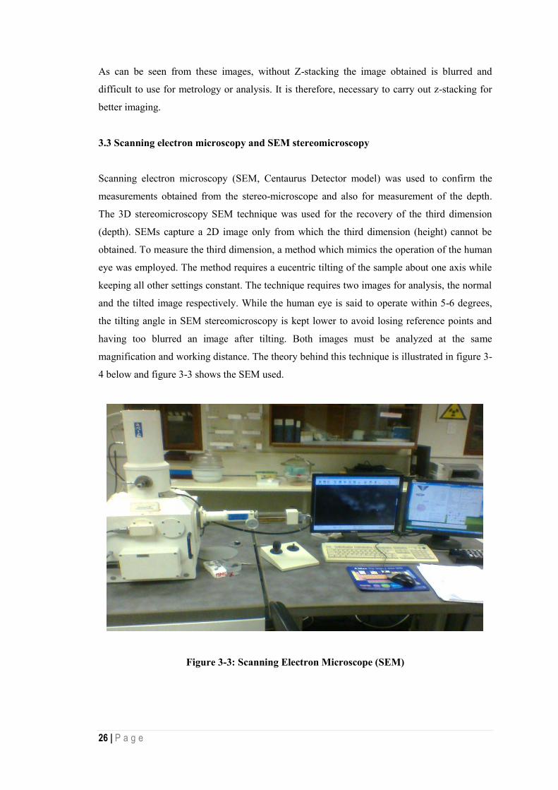
3.3 Scanning electron microscopy and SEM stereomicroscopy

Scanning electron microscopy (SEM, Centaurus Detector model) was used to confirm the

measurements obtained from the stereo-microscope and also for measurement of the depth.

The 3D stereomicroscopy SEM technique was used for the recovery of the third dimension

(depth). SEMs capture a 2D image only from which the third dimension (height) cannot be

obtained. To measure the third dimension, a method which mimics the operation of the human

eye was employed. The method requires a eucentric tilting of the sample about one axis while

keeping all other settings constant. The technique requires two images for analysis, the normal

and the tilted image respectively. While the human eye is said to operate within 5-6 degrees,

the tilting angle in SEM stereomicroscopy is kept lower to avoid losing reference points and

having too blurred an image after tilting. Both images must be analyzed at the same

magnification and working distance. The theory behind this technique is illustrated in figure 3-

4 below and figure 3-3 shows the SEM used.

Figure 3-3: Scanning Electron Microscope (SEM)

27 | P a g e

Electron Beam

Z

B’

Ө-α

X B

α Ө

A C’ C

Figure 3-4: 3D Stereomicroscopy

The projection of line AB on the focal plane will be AC. After tilting the sample an angle α,

point B moves to B’ while point A remains still. This is tilting about the Y axis. Then the

projection of line AB’ on the focal plane will be changed to AC’, which is observed as the

displacement of point B in two stereo pair images. This is called parallax movement. From

Figure 3-4, the following geometrical relationships can be derived:

From the sine rule of triangles and trigonometrical rations:

LAC

sinθ=

LAC′

sin(θ−α) and

LAC

LBC= tanθ (11)

LAC and LAC’ can be measured on the SEM images and the tilt angle is a known value. The

relative height LBC can be expressed as:

LBC =LACcosθ−LAC′

sinα (12)

When the tilt angle is small, Eq. (12) can be simplified as:

LBC =LAC−LAC′

2sin (α

2)

=P

2sin (α

2) (13)

Where, P is called the Parallax value.

Figure 3-5 below shows a cross section of the strand and the measured depth.

28 | P a g e

w

h

h

Figure 3-5: Fret mark depth

From the figure 3-5, it can be shown that, h is given by the equation:

h = Rw√{1 − (w

2Rw)2} (14)

Where;

Rw is the radius of the strand

w is the width of the fret mark

Figure 3-6 shows some of the micrographs used in third dimension (height) recovery.

The depth,‘d’ measured by the SEM stereomicroscopy is then;

d = a − h (15)

Where ‘a’ is the interference on one strand.

29 | P a g e

(a) Original position, 302.6microns

(b) Tilted position, 293.8micron

Figure 3-6: Micrographs used in Depth Measurement

30 | P a g e

3.4 Energy dispersive spectroscopy

Energy Dispersive Spectroscopy makes use of the X-ray spectrum emitted by a solid sample

bombarded with a focused beam of electrons to obtain a localized chemical analysis. All

elements from atomic number Z 4 (Be) to 92 (U) can be detected in principle, though not all

instruments are equipped for 'light' elements (Z < 10). Qualitative analysis involves the

identification of the lines in the spectrum and is fairly straightforward owing to the simplicity

of X-ray spectra. Quantitative analysis (determination of the concentrations of the elements

present) entails measuring line intensities for each element in the sample and for the same

elements in calibration Standards of known composition.

By scanning the beam in a television-like raster and displaying the intensity of a selected X-ray

line, element distribution images or 'maps' can be produced. Also, images produced by

electrons collected from the sample reveal surface topography or mean atomic number

differences according to the mode selected. The scanning electron microscope (SEM), which is

closely related to the electron probe, is designed primarily for producing electron images, but

can also be used for element mapping, and even point analysis, if an X-ray spectrometer is

added. There is thus a considerable overlap in the functions of these instruments.

In this research, EDS was extensively used to determine the elemental composition of the fret

mark surfaces before and after the fatigue testing.

3.4.1 Sample preparation

The samples used in EDS analysis, were not cleaned in any way so as to avoid rubbing off any

elements form the surfaces. The strand was cut into smaller pieces (less than 1cm long) and

fitted onto stubs. The samples where mounted on the stabs using the double sided tape. The

stubs were then mounted into the FEGSEM and screwed to prevent them from failing in case

of tilting. Eight (08) stubs were loaded in the FEGSEM per cycle. Figure 3-7 shows the

microanalysis of the fret mark surfaces.

For each fret mark, at least two points were analyzed for elemental composition and the results

from each scan averaged. This was done in order to get a true reflection of the elements

present on the surfaces. The report generated with the highest number of elements was used as

the reference spectrum. For other spectra with some of the elements not picked automatically,

the missing elements were manually picked and then, the percentages calculated.

31 | P a g e

Figure 3-7: EDS on fret mark surfaces

Figure 3-8 shows the FEGSEM used for the EDS analysis.

Figure 3-8: FEGSEM for Energy Dispersive Spectroscopy (EDS) Analysis

32 | P a g e

3.5 Tensile testing

Before starting the fatigue, the strands of the conductor samples were subjected to a tensile test

conducted at preformed line products (PLP). The certificate of the test results is attached in

annexure A.

3.6 Fatigue testing

The existing test rig of 95m long and suitably designed for the testing of the effectiveness of

dampers and conductor self-damping was used for the fatigue tests. The rig is equipped with

square faced conductor clamps. For fatigue testing of conductors, the test rig was modified to

suit the recommendations given by the following organisations and standards with regards to

fatigue testing:

(i) Cigre’ Working Group 11, Study Committee B2 Task force B2.11.07

(ii) Electrical Power Research institute(EPRI) Transmission lines Reference Book

(iii) International Electrotechnical Commission (IEC) 62568

(iv) IEEE 563

(v) The Planning, Design and Construction of overheard lines, Eskom Power Series

From all these references the following points were taken into consideration and employed for

the design of the test rig;

I. The use of a standard short (salvi) suspension clamp. The suspension clamp was tilted

at an angle between 5˚ and 10˚ in order to simulate the conductors exit angle due to

sagging at the suspension clamp in actual lines. The rig was designed with the tilt

angle set at 7˚. This angle was measured and confirmed with a protractor

II. The distance from the dead end of the conductor to the suspension clamp measured

horizontally must not be less than 2m. This is to ensure that the load is uniformly

distributed in the conductor strands.

III. The suspension clamp must be restricted from articulation during the tests to avoiding

its rocking motion in order to simplify the analysis.

IV. The distance of the point of attachment of the shaker to the conductor must be greater

than five (05) free vibrating loops from the suspension clamps to ensure uniform

solicitation of the strands in the area where fretting fatigue takes place.

V. The length of the active span of the conductors must be such that the wavelength of

the induced waveform is relatively bigger than the length of the clamp.

VI. The frequency of the shaker was chosen such that it excites the resonant mode of a taut

conductor.

33 | P a g e

VII. Characteristic catenary constant of Eskom power transmission lines. The tension was

maintained within ±2.5%.

With these conditions taken into consideration and using the following data for an ACSR-Tern

conductor, the design parameters for the test rig can be established.

Table 3-2 ACSR Tern Conductor Standard Parameters

Item Description Unit of Measure Quantity

Ultimate Tensile Stress kN 98.7

Mass per metre Kg/m 1.34

Diameter mm 27.0

Number of aluminium wires - 45

Number of Steel wires 7

Diameter of aluminium

wires

mm 3.38

Diameter of Steel wires mm 2.25

Modulus of Elasticity of

Steel

MPa 210,000

Modulus of Elasticity for

Aluminium(E-grade)

MPa 70,000

The design of the test rig entailed the determination of the following parameters using the data

from table 3-2 and meeting all the standard requirements;

(i) Resonant frequency(f)

(ii) Span Length(L)

(iii) Mode of the vibration(n)

These parameters were determined based on bending amplitude of 0.2mm -0.3mm.

These quantities are related by the Eq. (16):

𝑓𝑛 =𝑛

2𝐿√

𝑇

𝑚 (16)

Where:

34 | P a g e

T is the Tension

m is the linear mass

The Tension (T) is the Every Days Stress (EDS) in the conductor. This stress is determined

based on the conductor unit weight and a design constant called the catenary constant (C).

𝐶 =𝑇

𝑤 (17)

w is the weight per meter of the conductor in N/m

For phase conductors, Eskom uses a Catenary constant of 1800m. For a tern conductor this

will result in an EDS of 23.66kN (23.97% of UTS).

Inserting this data into eq. (16) yields:

𝑓𝑛 =𝑛

2𝐿√

23660

1.34=

66.439𝑛

𝐿 (18)

𝑓𝑛 =66.439𝑛

𝐿 ,𝑛

𝐿= 0.9031 (19)

The relationship between the wavelength, span and mode of a standing wave is given by Eq.

(20):

𝑛

𝐿=

2

𝜆 (20)

From Eq. (19) and Eq. (20) we get:

𝜆 ≤ 2.214𝑚

Taking the wavelength to be 2.2m, then n/L = 0.9091, giving a frequency of 60.4Hz from

Eq. (20).

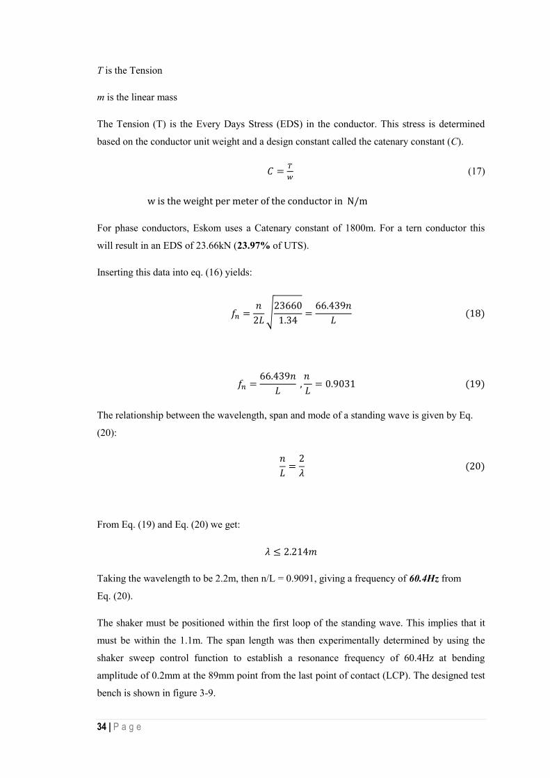
The shaker must be positioned within the first loop of the standing wave. This implies that it

must be within the 1.1m. The span length was then experimentally determined by using the

shaker sweep control function to establish a resonance frequency of 60.4Hz at bending

amplitude of 0.2mm at the 89mm point from the last point of contact (LCP). The designed test

bench is shown in figure 3-9.

35 | P a g e

During the fatigue testing the temperature was maintained to below 21֯C at all times. The lab is

equipped with air conditioners and thermocouples to regulate the temperature to the required

value.

36 | P a g e

Suspension Clamp

Strip Strain gauges

Dead weights

Cell Strand breakage detection mechanism End Clamp

ACSR conductor 2m

7˚

Shaker Laser sensor

Figure 3-9: (a) Resonance fatigue testing bench

Concrete Foundation

DAQ Puma Control

System

Steel

stand Concrete Block

CPU-1 CPU-2

Monitor-

1(LAB VIEW)

Monitor-

2(VIP)

37 | P a g e

Figure 3-9: (b) Fatigue test set-up at VRTC-UKZN

3.6.1 Conductor Sample preparation

The samples used in this research were supplied by Aberdare to Eskom. Some of the drums

were rejected by Eskom due to quality issues and were then forwarded to the Vibration

Research and Testing Centre (VRTC) for analysis.

The conductors samples were pulled into the lab from the backyard. End fittings (compression

type) were then fitted to the conductors using a crimping machine. The correct dies for the

Tern conductor were selected from the crimping chart.

The Tern conductor sample was then strung onto the test bench. The sag angle on the clamp

was set to 7° and the tension adjusted to 23.66kN. The bolts on the clamp were tightened to the

recommended 40kN-m for the Salvi clamp.

38 | P a g e

3.6.2 Bending amplitude measurement

The bending amplitude is an important parameter in fatigue testing of transmission line

conductors. It is a parameter which is commonly used to benchmark the performance of the

conductor. In this research, it was required that the bending amplitude be kept with the

endurance capability of multilayer ACSR conductors, which is 0.2mm-0.3mm at a point 89mm

from the last point of contact between the conductor and the clamp(LCP).

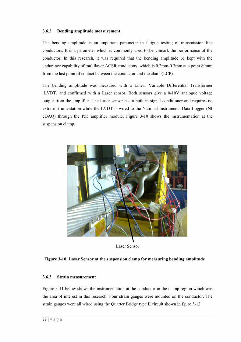
The bending amplitude was measured with a Linear Variable Differential Transformer

(LVDT) and confirmed with a Laser sensor. Both sensors give a 0-10V analogue voltage

output from the amplifier. The Laser sensor has a built in signal conditioner and requires no

extra instrumentation while the LVDT is wired to the National Instruments Data Logger (NI

cDAQ) through the P55 amplifier module. Figure 3-10 shows the instrumentation at the

suspension clamp.

Laser Sensor

Figure 3-10: Laser Sensor at the suspension clamp for measuring bending amplitude

3.6.3 Strain measurement

Figure 3-11 below shows the instrumentation at the conductor in the clamp region which was

the area of interest in this research. Four strain gauges were mounted on the conductor. The

strain gauges were all wired using the Quarter Bridge type II circuit shown in fgure 3-12.

39 | P a g e

98.5mm

1 2 3

Clamp keeper 93mm

LCP ACSR Conductor

Strain gauges Accelerometer (89mm point)

Figure 3-11: Arrangement of strain gauges at the mouth of the clamp

The diagram above, the first strain gauge was positioned at 15.2mm from the clamp keeper.

The second, third and fourth were positioned at; 32.9mm, 62.1mm and 95.6mm from the first

one respectively. On the upper part of the conductor, four gauges were installed. An

accelerometer was mounted at 89mm point from the LCP on the bottom side of the conductor.

The accelerometer was first mounted on a calibrator and it sensitivity tested in both the upward

and downward positions at both 41Hz and 69Hz. The accelerometer did not show any

sensitivity change with regards to the mounting directions. The output from the gauges was

logged by a data logger and analysed with Microsoft excel and Matlab in graphical form. The

results from the strain gauges were used to plot the stress distribution in the clamp region and

compare with available theoretical models. Figure 3-12 below show the quarter bridge type II.

The characteristics of the strain gauges used in the analysis are shown in table 3-3.

The quarter bridge type two configuration uses a single active, plus a passive or “dummy”

gauge mounted transverse to the active gauge or on another piece of material as the component

whose strain is to be measured. The dummy gauge does not measure any strain but is provided

for the purposes of temperature compensation only. The applied strain will have very little

influence on the dummy gauge as it is mounted perpendicular to the active gauge. Temperature

changes will however have the same effect of both the active and dummy strain gauges and

will cancel each other out in the balanced Wheatstone bridge. The strain measured by this

bridge configuration is given by:

40 | P a g e

휀 = −4𝑉𝑟 ∗

1 +𝑅𝑙𝑅𝑔

[𝐺𝐹 ∗ (1 + 2𝑉𝑟)] (21)

Where:

Rl is the Lead wire resistance

Rg is the Nominal strain gauge resistance

GF is the Gauge factor of the strain gauge and is defined as the relationship between the

resultant fractional change in gauge resistance to the applied strain (fractional change in

length). It is given by the equation below:

𝐺𝐹 =

∆𝑅𝑅∆𝑙𝑙

=

∆𝑅𝑅휀

(22)

휀 is the measured strain (in micro-strains)

Vr is given by:

𝑉𝑟 =𝑉0 (𝑠𝑡𝑟𝑎𝑖𝑛𝑒𝑑) − 𝑉0(𝑢𝑛𝑠𝑡𝑟𝑎𝑖𝑛𝑒𝑑)

𝑉𝑒𝑥 (23)

V0 (strained) is the bridge output voltage for a strained component

V0 (Unstrained) is the bridge output voltage for an unstrained component

Vex is the excitation voltage.

The strain measurement with this bridge type is independent of the poison’s ratio.

The resistances given in table 3-3 is the series sum of individual resistance of active gauge and

the dummy (each gauge has a resistance of 350 Ohms).

In the set-up used in this research, the dummy gauges were mounted separately on an

aluminium bar which was then suspended in the vicinity of the suspension clamp.

Before connecting the strain gauges to the system, calibration was carried out. The calibration

is aimed at ensuring that the system resistor, R1 and R2 are equal and of the correct value.

41 | P a g e

Rl

R1 Rg

Rl

Vo

R2

Rl Rg (dummy)

Figure 3-12: Quarter bridge configuration

Table 3-3 Characteristics of the strain gauges

Strain Gauge No. Initial Resistance(Ohms) K(Sensitivity)

1 700 2.07

2 699 2.15

3 699 2.15

4 700 2.07

3.6.4 Strand breakage detection mechanism

The strand breakage detection mechanism employed a non-contact displacement detection

sensor and National Instruments (cDAQ) data logger. This system basically operates based on

the torsional effects of stranded conductors. Depending on the lay direction of the layer in

which the broken strand is located, the conductor will rotate through a certain angle due to the

redistribution of the tangential component of the conductor tension in the strands. The

direction of rotation the conductor of the mechanism also indicates the layer in which the

strand has failed (broken). An aluminium blade was attached to the conductor by means of

VDC

----

----

-

42 | P a g e

bolting it to the clamp which was then bolted on the conductor. The laser sensor was used to

measure the distance of the aluminium strip from the sensors per cycle and the signal sent to

the data logger. The recorded signal was a plot of displacement versus time. If any strand

breaks, the conductor will twist through some angle and the aluminium strip will change its

position. The laser sensor will pick this abrupt change as a spike and change in average value

in the output signal. The data logger used had enough memory to store up to 100 million

cycles. The entire assembly was designed in such a way that its weight had minimal effect on

the entire conductor-clamp vibrating system.

α X1

Laser Sensor

Aluminium Blade

Figure 3-13: Strand breakage detection mechanism

When a strand breaks, the entire assembly will rotate about the longitudinal axis of the

conductor so that the vertical axis is shifted through some angle α. The non-contact

displacement sensor will record a new displacement(x1). The mechanism was clamped to the

conductor at the node so that it experiences minimal vibration. A laser sensor model

LG5B65PU (borrowed from Aberdare) was used for this mechanism.

NI cDAQ

43 | P a g e

3.6.5 Frequency sweep

To determine the actual resonant frequency, a frequency sweep was done from 0 to 100Hz.

Two resonance frequencies were identified, 41 Hz and 69Hz. The 41 Hz frequency

corresponded to the frequency calculated from the Eq. (8) with a wind speed of 6m/s as

Aeolian vibrations occur for wind speeds between 1-6m/s for single conductors (High Voltage

Overhead Power Lines- Theoretical Calculations and Formulae for Conductor Installations,

2009) and was therefore used to test sample number 1, in order to try and simulate the natural

conditions. The second sample was tested at 69Hz in order to reduce the testing time. Figure 3-

14 shows a sample frequency sweep for conductor sample number 1. The frequency sweep

was run using the PUMA control system.

Figure 3-14: Frequency sweep

3.6.6 Fatigue testing

A LabVIEW program, shown in figure 3-15 below, was used to log all the required data and for monitoring the bending amplitude. The following data was logged:

The bending amplitude Acceleration at the 89mm point

Strain measurements from all strain gauges

Displacement from strand breakage mechanism

The Butterworth low pass filters were used to filter the signals and frequency measured using a

tone block. The control of the bending amplitude was done manually. An indicator which

0

0,1

0,2

0,3

0,4

0,5

0,6

0,7

0,8

0,9

64 65 66 67 68 69 70 71

Vol

tage

Frequency

Frequency Sweep

44 | P a g e

showed a green light when the bending amplitude is within the correct value and red when it is

out of range was designed into the circuit for easy monitoring of the bending amplitude. The

PUMA control system as well as the Vibration interactive program were used to counter check

the measurements obtained using LabVIEW.

The temperature in the clamp region was constantly monitored using a FLIR thermos-camera

to ensure that it were below 100°C, the temperature at which annealing is expected to occur for

aluminium strand.

A screen shot of the data logged is shown in figure 3-16.

Figure 3-15: LabVIEW program

45 | P a g e

Figure 3-16: Indicators for Amplitude monitoring

3.7 Fractography

After the fatigue testing of the conductor samples, fractographic analysis was carried out to

establish whether the cracks had nucleated and the sites from where they nucleated. During

this analysis the stands were not cleaned in order to avoid rubbing off micro-cracks. A

conductor sample from the last point of the clamp keeper on the dead end side to the first

antinode was cut and subjected to fractographic analysis.

3.7.1 Stereomicroscopy

The strands were first checked for any cracks using stereomicroscopy. After identification of

fractured surfaces or cracked surfaces, the points of interest were cut into smaller specimens

and mounted on the stub for detailed analysis in the SEM. Before being cut into smaller pieces,

the distance of the cracks of interest from the front end of the clamp keeper was measured and

recorded. The distance measure was the linear distance as the strands were straightened. The

actual distance can be calculated by making use of the equation for calculating the length of a

helix given as:

𝑙 = √(𝜋𝐷)2 + 𝑃2 (24)

This is the length of one turn of a helix. If the measured linear distance for the location of the

crack is ‘x’, then the actual distance (x’) is given by:

46 | P a g e

𝑥′ =𝑥

𝑙∗ 𝑃 (25)

Where:

D is the mean diameter or pitch

P is the lay length

3.7.2 Scanning Electron Microscopy

The scanning electron microscope was used to measure the sizes of the cracks which had

nucleated and propagated.

3.7.3 Energy Dispersive microscopy

The Field Emission Gun Scanning Electron microscope (FEGSEM) was used for determining

the elemental composition of the fractured surfaces. The target element was oxygen which

would prove the presence of aluminium oxide, which is associated with the fretting fatigue of

aluminium conductors.

47 | P a g e

4. Data Collection, Collation and Analysis

4.1 Stereomicroscopy and scanning electron microscopy

From the surface characterization carried out using stereomicroscopy and electron

microscopy, the dimensions of the fret marks were collected and collated in table 4-1.

In this table, the layer from which the strands were selected is indicated. The strand number

and fret mark numbers are also indicated. For the middle and inner layer, the fret mark position

is also specified i.e. top or bottom.

The initial depth is the calculated depth, h shown in figure 3-5 and is dependent on the width

of the fret mark. The length L1 and L2 refer to the measured length in the tilted and un-tilted

position of the specimen. The tilt angle is the angle through which the specimen is rotated at

constant working distance and magnification for recovery of the third dimension.

As can be seen from the table, some depths appear as negative values. This is because the

method used for depth measurement measures the relative depth between two points.

Therefore if the reference point is above the point of interest, a positive value results otherwise

a negative value will result. All the negative values were converted to a positive value called

the mod depth (modulus).

Four points were analyzed per strand and the strands sampled as per SANS 182-2. For strands

with fret marks on both the top and bottom sides, this resulted into eight points per strand.

The challenge with using the SEM method for depth measurement was mostly the

identification of the same key features in both the normal and the tilted specimen. If the

features are slightly missed, the results will be out of range and it depends on the experience

and skill of the individual carrying out the experiment to judge whether the result is valid or

invalid.

The other challenge with this method is that it is time consuming and would require the

equipment dedicated to it. On average, it took about 30 minutes to successfully analyze a

single fret mark on the SEM.

The total depth is the overall indentation depth on the strand. The relative depth is a ratio

between the total depth and diameter of the strand. The measured conductor parameters are

given in the analysis section. Figure 4-1 shows micrographs from the SEM.

48 | P a g e

Table 4-1: Results from SEM and stereomicroscopy for sample 1

Layer Strand No. Mark Length Width L1 L2 Tilt Angle Depth Mod Depth Initial Depth Total Depth Relative Depth

1 1449 298,3 171,9 179,2 4,7 89,017 89,017 3,297 92,314 0,027

2 706,6 266,7 125 177,1 4,7 635,310 635,310 2,635 637,946 0,189

3 2169,3 652,08 183,4 182,9 2 -14,325 14,325 15,785 30,110 0,009

4 1867 460,1 380,9 387,1 2,4 148,025 148,025 7,850 155,875 0,046

1 1226 202 236,5 241,4 1,9 147,770 147,770 1,512 149,282 0,044

2 1995 395,4 289,8 296,6 1,4 278,302 278,302 5,795 284,097 0,084

3 2290 465,4 217,7 220,6 1,7 97,744 97,744 8,032 105,775 0,031

4 2080 498,8 462,2 470,1 2 226,331 226,331 9,227 235,558 0,070

1 1953 413,8 219,6 229,2 7,6 72,427 72,427 6,348 78,775 0,023

2 2997 506,2 279,1 293,8 5 168,504 168,504 9,504 178,007 0,053

3 2227 311,4 1101 1131 2,7 636,681 636,681 3,593 640,274 0,190

4 1638 355 922,3 939 2,1 455,665 455,665 4,671 460,336 0,136

1 2217 505,9 390,8 393,7 2,3 72,248 72,248 9,492 81,740 0,024

2 1554 274,2 170,5 173,3 2,9 55,326 55,326 2,786 58,112 0,017

3 2804 485 490,3 477 2 -381,038 381,038 8,723 389,761 0,115

4 3141 487,8 175,9 170,5 2,7 -114,603 114,603 8,824 123,427 0,037#DIV/0! #DIV/0! 0,000 #DIV/0!

1 2379 499,6 1113 1098 2 -429,742 429,742 9,257 438,999 0,130

2 2241 418 276 273,4 2,4 -62,075 62,075 6,477 68,553 0,020

3 2551 391,7 1365 1352 2,1 -354,709 354,709 5,687 360,397 0,107

4 1652 504,6 894,3 885,9 1,8 -267,392 267,392 9,444 276,836 0,082

1 2117 266,1 159,8 165,8 2,6 132,233 132,233 2,624 134,856 0,040

2 2713 335,1 563 553 1,4 -409,267 409,267 4,162 413,429 0,122

3 2817 552,5 908,8 904,8 2,1 -109,141 109,141 11,325 120,466 0,036

4 2428 446,3 1189 1208 2,4 453,626 453,626 7,385 461,012 0,136

1 2068 421,9 195,3 197,9 2,6 57,301 57,301 6,599 63,900 0,019

2 2090 516,2 205,6 208,9 2,5 75,637 75,637 9,883 85,520 0,025

3 3331 649,3 369,2 394,7 2,5 584,465 584,465 15,651 600,116 0,178

4 1759 278,9 175,2 178,6 2,2 88,554 88,554 2,882 91,436 0,027

1 2910 518,8 328,5 332,3 2,6 83,747 83,747 9,983 93,731 0,028

2 2122 362,5 402,8 413,2 2,2 270,870 270,870 4,870 275,741 0,082

3 2207 359,5 690,5 699,6 2,1 248,297 248,297 4,790 253,087 0,075

4 2175 268,7 151,5 158,9 2,6 163,087 163,087 2,675 165,762 0,049

1 1288 300,5 254,9 263,5 2,3 214,252 214,252 3,346 217,598 0,064

2 3155 616,1 505,2 500 4,4 -67,730 67,730 14,088 81,818 0,024

3 2881 556,7 368,8 365,2 3,5 -58,942 58,942 11,498 70,440 0,021

4 1263 393,8 112,4 114,6 2 63,029 63,029 5,749 68,777 0,020

1 2433 438,6 593,1 583 2,1 -275,582 275,582 7,132 282,714 0,084

2 2321 355,9 303,3 313,4 2,7 214,349 214,349 4,695 219,044 0,065

3 3439 522,3 290,7 293,4 2,3 67,265 67,265 10,119 77,384 0,023

4 3081 405,8 583 589,8 2,8 139,161 139,161 6,105 145,266 0,043#DIV/0! #DIV/0! 0,000 #DIV/0! #DIV/0!

1 1865 438,6 1116 1102 1,9 -422,200 422,200 7,132 429,333 0,127

2 2426 544,8 155 148,3 2 -191,951 191,951 11,011 202,962 0,060

3 2320 518,9 252,8 249,4 2,5 -77,929 77,929 9,987 87,916 0,026

4 1983 480,5 322,1 315,9 2,4 -148,025 148,025 8,562 156,587 0,046

1 2801 690,3 495 490,4 4 -65,904 65,904 17,695 83,599 0,025

2 1797 403,2 109,9 102,9 1,1 -364,616 364,616 6,027 370,643 0,110

3 2149 341,8 506,1 503,1 3,2 -53,722 53,722 4,330 58,052 0,017

4 1827 367 339,3 332,5 1,4 -278,302 278,302 4,992 283,294 0,084

1 1949 454,2 140 143,2 2,3 79,722 79,722 7,649 87,371 0,026

2 2838 409,6 296,6 286,5 2,2 -263,057 263,057 6,220 269,276 0,080

3 1659 362,8 464,7 467,9 2,5 73,345 73,345 4,878 78,223 0,023

4 1731 334,9 782 776,3 2 -163,302 163,302 4,157 167,458 0,050

1 1726 296 397,7 401 1,7 111,226 111,226 3,247 114,472 0,034

2 2371 384,2 961 972,1 1,8 353,340 353,340 5,471 358,811 0,106

3 2115 727,2 169,9 173,9 1,9 120,629 120,629 19,643 140,272 0,042

4 2416 413,1 242,6 249,4 2,5 155,857 155,857 6,326 162,184 0,048

Inner

1-Top

1-Bottom

2-Top

2-Bottom

Outer

1-Bottom

1-top

2-Top

2-Bottom

Mid-Layer

1

2

3

4

3D SEM Stereomicroscopy

3-Top

3-Bottom

49 | P a g e

(a) Strand 1

(b) Strand 2

Figure 4-1: Measuring the axes of the fret marks

50 | P a g e

(a) Untilted Position

(b) Tilted Position

Figure 4-2: SEM 3D Stereomicroscopy

51 | P a g e

(a) Fret mark at the core to inner layer contact

(b) Fret mark on the outer layer

Figure 4-3: Micrographs used for measurements

52 | P a g e

Table 4-2 shows a summary of the microscopy results for sample one, bottom of strand fret

marks. The fret mark size (area) increases as you move into the inner layers. The marks are

largest (in terms of the major and minor axes) in the middle layer bottom side of the

strands. The depth is the largest in the outer layer followed by the inner layer and smallest

in the middle layer for the analyzed samples. The depth on the other hand reduces

progressively from the outer layer to the inner layer. The cable designer must therefore aim

at reducing the depth in the outer layer and the surface area in the middle layer.

Table 4-2 summary of fret mark dimensions for sample 1 bottom side of strands

Sample 1

Contact pair Length Width Depth Area Eccentricity

Outer/ Mid-layer 2019.62 411.13 231.34 2.61E+06 0.979

Mid/Inner Layer 2459.25 420.50 221.46 3.25E+06 0.985

Inner/Core 2150.00 450.85 196.42 3.05E+06 0.978

4.2 Fatigue testing results

The samples were subjected to 50 and 40 million fatigue cycles respectively. The first sample

was fatigue tested at 41Hz to simulate the natural Aeolian vibration conditions in the South

African environmrnent. The second sample was tested at 69 Hz. This was an accelerated

fatigue test with all other conditions set as in the testing of sample 01. Annexure D shows a

record of the fatigue test for sample 01.

The test took about 3.5 months to achive 50.9 million cycles at 41 Hz reprenting a life of 25

years in service. The biggest challenge was the unavailability of the laboratory after working

hours. The test could only be run from 08:00 hours to 16:00 hours. The second conductor

sample was exposed to 40 million fatigue cycles.

4.2.1 Bending of the Conductor in the salvi clamp region

The bending strain and hence stress of the conductor in the clamp region was investigated and

compared to the available models in the this section. Figure 4-4 shows the strains obtained

from the experiments and the ones calculated from the PS equation.

53 | P a g e

Figure 4-4: Bending Strains on the upper surface of the conductor

The bending strain in the clamp region of a square faced clamp is given by the equations below;

𝜎𝑏 = 𝐾𝑌𝑏 (26)

𝜎𝑏 = 𝐸𝑎휀𝑏 (27)

The conversion factor K is given by the Poffenberger-Swart (PS) formula and is dependant

upon distance from the clamp, the material and design of the conductor.

𝐾 =𝐸𝑎𝑑𝑝2

4 ∗ (𝑒−𝑝∗𝑥 − 1 + 𝑝 ∗ 𝑥) (28)

Therefore the strain is given by:

휀𝑏 =𝑑. 𝑝2

4 ∗ (𝑒−𝑝∗𝑥 − 1 + 𝑝 ∗ 𝑥)𝑌𝑏 (29)

Yb is the bending amplitude peak to peak in mm

Ea is the modulus of Elastic of an outer strand wire

-5,00000

95,00000

195,00000

295,00000

395,00000

495,00000

595,00000

695,00000

795,00000

895,00000

0 5 10 15 20 25 30 35 40 45 50 55 60 65 70 75 80 85 90 95 100

Ben

din

g st

rain

(m

icro

stra

in)

Distance from clamp keeper(mm)

Bending strain vs distance

Bending Strain -71Hz (microstrains) Bending Strain-41Hz

Bending strain -PS Equation

54 | P a g e

𝜎𝑏 is the bending stress ( 0 to peak)

휀𝑏 is the corresponding bending strain

d is the diameter of the outer strand

T is the conductor tension

E*I is the sum of the flexural rigidity of the individual conductor strands

𝑝2 =𝑇

𝐸 ∗ 𝐼

x is the distance of measurement from the last point of contact (LCP)

The PS equation gives strains which are lower than the measured valued for this set-up. The

peak stress was however closer to that measured at 71Hz as the PS equation value has to be

doubled( the PS equation calculates the peak strain while the measured strain is the peak to

peak).

The bending strain at 41Hz can be approximated by a quadratic equation below with a

regression constant of 0.9977:

휀 = 0.2152𝑥2 − 29.266𝑥 + 1025 (30)

The strains measured at 71Hz can be modelled by the following equation;

휀 = 0.0021𝑥3 + 0.3387𝑥2 − 16.773𝑥 + 409.62 (31)

4.3 Energy dispersive spectroscopy

The results from the Energy dispersive spectroscopy (EDS) are shown in the reports in

annexure B. Each report contains a table showing the percentage weight of elements on the

surafces of the fret marks, the image and the spectrum. These reports were generated on the

FEGSEM.

The results from all the reports are summarized in the table 4-3. It is worth noting that there is

a high Zinc content on the surfaces of the fret marks in the inner most layer. There is transfer

of Zinc from the galvanized steel wires in the core to the inner layer aluminum wires.

55 | P a g e

Table 4-3: Summary of EDS results

Layer Position Al O C Si K Ca Zn Fe Total Trace

82,8 15,93 0 0,55 0,06 0,07 0 0,24

28,9 19,04 7,93 0,08 0,01 0,01 44,04 0

55,85 17,485 3,965 0,315 0,035 0,04 22,02 0,12 99,83 0,17

64,48 23,36 0 0,01 0,03 0 11,7 0

34,15 17,04 0 0,11 0,01 0 48,55 0

49,315 20,2 0 0,06 0,02 0 30,125 0 99,72 0,28

65,76 7,745 25,11 0,67 0,2 0,6 0 0,245

61,19 8,32 28,24 0,97 0,2 0,2 0 0,41

63,475 8,0325 26,675 0,82 0,2 0,4 0 0,3275 99,93 0,07

89,85 8,33 0 0,66 0 0,17 0 0,4

91,68 7,52 0 0,19 0,04 0 0 0,2

90,765 7,925 0 0,425 0,02 0,085 0 0,3 99,52 0,48

67,31 19,35 11,32 0,13 0 0 0 0,17

78,92 11,67 3,46 3,98 0,22 0,15 0 0,87

73,115 15,51 7,39 2,055 0,11 0,075 0 0,52 98,775 1,225

BottomOuter Layer

Top

Bottom

Inner Layer

Mid-Layer

Top

Bottom

56 | P a g e

4.4 Fractography

4.4.1 Nucleation and propagation of cracks

The strand surfaces were examined as explained in the methodology section of this thesis.

Micro cracks were observed to have nucleated but in most cases not a critical length or depth.

Most of the cracks are observed to be transverse to the major axis of the fret marks. Figure 4-3

shows some of the examined surfaces after the fatigue testing. In most cases the cracks had

nucleated from the fret marks. In very rare cases were the cracks observed to have nucleated

from other defects such as scratches. The longest observed crack was about 14.3% of the

diameter of the aluminum strand.

(a) 217.9micron crack on surface

57 | P a g e

(b) 270.4 microns crack

(c ) Multiple cracks on surface of fret mark

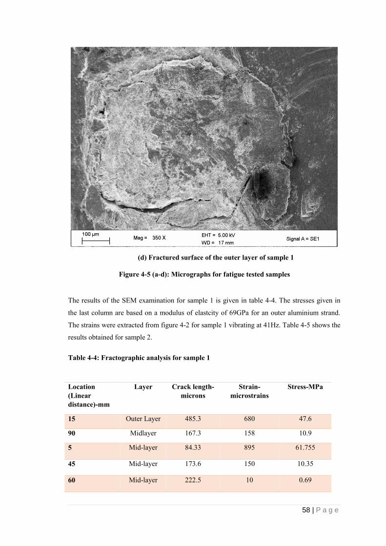
58 | P a g e

(d) Fractured surface of the outer layer of sample 1

Figure 4-5 (a-d): Micrographs for fatigue tested samples

The results of the SEM examination for sample 1 is given in table 4-4. The stresses given in

the last column are based on a modulus of elastcity of 69GPa for an outer aluminium strand.

The strains were extracted from figure 4-2 for sample 1 vibrating at 41Hz. Table 4-5 shows the

results obtained for sample 2.

Table 4-4: Fractographic analysis for sample 1

Location (Linear distance)-mm

Layer Crack length-microns

Strain-microstrains

Stress-MPa

15 Outer Layer 485.3 680 47.6

90 Midlayer 167.3 158 10.9

5 Mid-layer 84.33 895 61.755

45 Mid-layer 173.6 150 10.35

60 Mid-layer 222.5 10 0.69

59 | P a g e

Location (Linear distance)-mm

Layer Crack length-microns

Strain-microstrains

Stress-MPa

60 Mid-layer 102.9 10 0.69

85 Mid-layer 176.8 115 7.935

80 Mid-layer 115.1 75 5.175

90 Mid-layer 81.19 165 11.385

25 Inner Layer 61.59 475 32.775

34 Inner Layer 44.87 315 21.735

60 Inner Layer 266.9 10 0.69

Table 4-5: Fractographic analysis for sample 2

Location (Linear distance)-mm

Layer Crack length-microns

Strain-microstrains

Stress-MPa

5 Outer Layer 170.9 350 24.15

24 Outer Layer 97.5 208 14.352

50 Outer Layer 270.4 150 10.35

20 Outer Layer 111.0 238 16.42

47 Outer Layer 53.71 142 9.80

10 Outer Layer 60 310 21.39

37 Outer Layer 118.1 142 9.80

55 Outer Layer 147.6 160 11.04

25 Mid-layer 43.96 206 14.21

93(89mmpoint) Mid-layer 219.1 30 2.07

7 Mid-layer 99.06 335 23.12

30 Mid-layer 105.6 170 11.73

45 Inner Layer 104.4 140 9.66

20 Inner Layer 138.0 238 16.42

60 | P a g e

Location (Linear distance)-mm

Layer Crack length-microns

Strain-microstrains

Stress-MPa

21 Inner Layer 130.0 230 15.87

59 Inner Layer 44.86 168 11.59

44 Inner Layer 61.00 140 9.66

35 Inner Layer 88.74 142 9.80

The stress calculated in most cases is higher than the Electrical Power Research Institute

(EPRI) quoted endurance capability for a multilayer conductor of 8.5N/mm2. Meaning that

theoretcially the conductor can not endure 500 million cycles. The bending strain measured at

the 89mm point in the test carried out at 41Hz was 200 microstrains which corresponds to the

IEEE recommended enduarance capability for multilayer conductors. Note that the position of

gauges in the table were measured relative to the clamp keep and not the LCP. Therefore, the

89mm point is actually at 93mm from the clamp keeper. Fig. 4-2 was used for extracting the

strain values.

4.5 EDS on fatigue tested samples

The results of the EDS on fatigue tested samples on the fret marks are presented below.

Sample reports per layer are given for illustration purposes only. The results from all the

reports are collated in table 4-6 below.

Table 4-6: EDS on fatigue tested samples

Layer Position Al O C Si K Ca Zn Fe Total Trace

Top 94,91 4,83 0 0,26 0 0 0 0 100 0

71,7 15,48 9,56 2,76 0,11 0 0 0,4

88,69 10,48 0 0,3 0,11 0 0 0,21

80,195 12,98 4,78 1,53 0,11 0 0 0,305 99,9 0,1

Top 76,14 17,37 0 5,72 0,15 0 0 0,5 99,88 0,12

77,51 7,93 10,15 0.31 0 0 0 0,2

64,86 11,2 13,88 0,07 0 0 13,45 0

71,185 9,565 12,015 0,035 0 0 6,725 0,1 99,625 0,375

74,07 7,65 17,69 0,23 0 0 0 0,26

90,74 6,92 0 1,87 0 0,02 0 0,45

82,405 7,285 8,845 1,05 0 0,01 0 0,355 99,95 0,05

Inner Layer

Mid-Layer

Outer Layer

Bottom

Bottom

Bottom

61 | P a g e

The results from the EDS analysis can be summarised in the histogram below. The analysis is

carried out per layer to show the elemental changes per layer. Figure 4-4 (a) to (d)

(a) Inner Layer top fret marks

(b) Inner Layer Bottom fret marks

0

20

40

60

80

100

120

Al O C Si K Ca Zn Fe Total Trace

Inner Layer Top

Before After

0

20

40

60

80

100

120

Al O C Si K Ca Zn Fe Total Trace

Inner Layer Bottom

Before After

62 | P a g e

(c) Middle layer top fret marks

(d) Mid-Layer Bottom fret marks

0

20

40

60

80

100

120

Al O C Si K Ca Zn Fe Total Trace

Mid-Layer Top

Before After

0

20

40

60

80

100

120

Al O C Si K Ca Zn Fe Total Trace

Mid-Layer Bottom

Before After

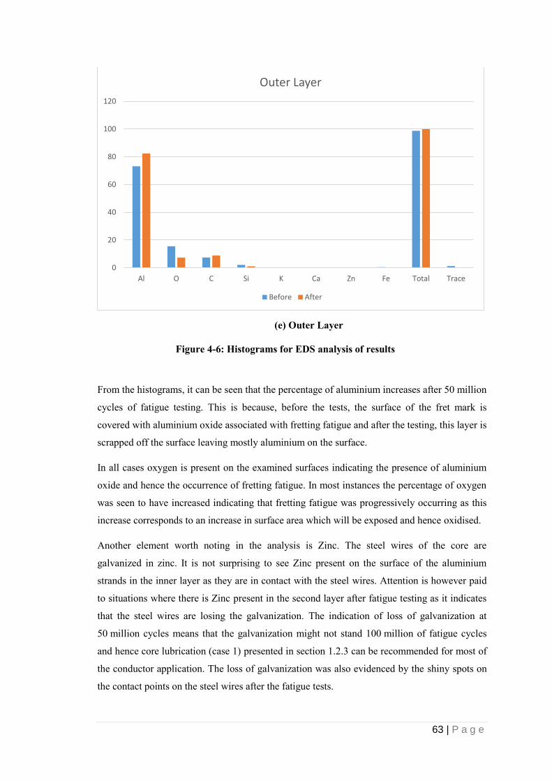
63 | P a g e

(e) Outer Layer

Figure 4-6: Histograms for EDS analysis of results

From the histograms, it can be seen that the percentage of aluminium increases after 50 million

cycles of fatigue testing. This is because, before the tests, the surface of the fret mark is

covered with aluminium oxide associated with fretting fatigue and after the testing, this layer is

scrapped off the surface leaving mostly aluminium on the surface.

In all cases oxygen is present on the examined surfaces indicating the presence of aluminium

oxide and hence the occurrence of fretting fatigue. In most instances the percentage of oxygen

was seen to have increased indicating that fretting fatigue was progressively occurring as this

increase corresponds to an increase in surface area which will be exposed and hence oxidised.

Another element worth noting in the analysis is Zinc. The steel wires of the core are

galvanized in zinc. It is not surprising to see Zinc present on the surface of the aluminium

strands in the inner layer as they are in contact with the steel wires. Attention is however paid

to situations where there is Zinc present in the second layer after fatigue testing as it indicates

that the steel wires are losing the galvanization. The indication of loss of galvanization at

50 million cycles means that the galvanization might not stand 100 million of fatigue cycles

and hence core lubrication (case 1) presented in section 1.2.3 can be recommended for most of

the conductor application. The loss of galvanization was also evidenced by the shiny spots on

the contact points on the steel wires after the fatigue tests.

0

20

40

60

80

100

120

Al O C Si K Ca Zn Fe Total Trace

Outer Layer

Before After

64 | P a g e

5. Contact Mechanics

The mathematical theory for the general three-dimensional contact problems was first given by

Hertz (1881). There is an extensive Hertzian theory which includes both stress and strain and

strain analysis together with a comprehensive bibliography has been published by Lubkin

(1962).

5.1 General Theory

The assumption is made that the surfaces in contact are perfectly smooth, that the bodies are

isotropic and linearly elastic, that the elastic limit of the materials is not exceeded and that

frictional forces are absent. The finite force keeping them together will then be distributed over

the common area of contact. The surfaces of the bodies will be assumed to be of second

degree, implying that all the terms higher than two in the surface equations will be neglected.

If two bodies are in mathematical contact (touching but unstressed and not deformed) so that

the common normal is parallel to the applied load, the common tangent plane is the plane xy

and the common normal is the z as shown in figure 5-1 below.

Figure 5-1: Two dimensional bodies in mathematical contact

(Source: Johnson, K. L., 1985)

The general equation of a surface of second degree is given by:

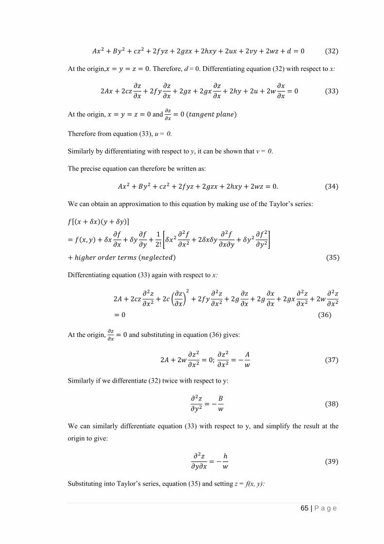
65 | P a g e

𝐴𝑥2 + 𝐵𝑦2 + 𝑐𝑧2 + 2𝑓𝑦𝑧 + 2𝑔𝑧𝑥 + 2ℎ𝑥𝑦 + 2𝑢𝑥 + 2𝑣𝑦 + 2𝑤𝑧 + 𝑑 = 0 (32)

At the origin,𝑥 = 𝑦 = 𝑧 = 0. Therefore, d = 0. Differentiating equation (32) with respect to x:

2𝐴𝑥 + 2𝑐𝑧𝜕𝑧

𝜕𝑥+ 2𝑓𝑦

𝜕𝑧

𝜕𝑥+ 2𝑔𝑧 + 2𝑔𝑥

𝜕𝑧

𝜕𝑥+ 2ℎ𝑦 + 2𝑢 + 2𝑤

𝜕𝑥

𝜕𝑥= 0 (33)

At the origin, 𝑥 = 𝑦 = 𝑧 = 0 and 𝜕𝑧

𝜕𝑥= 0 (𝑡𝑎𝑛𝑔𝑒𝑛𝑡 𝑝𝑙𝑎𝑛𝑒)

Therefore from equation (33), u = 0.

Similarly by differentiating with respect to y, it can be shown that v = 0.

The precise equation can therefore be written as:

𝐴𝑥2 + 𝐵𝑦2 + 𝑐𝑧2 + 2𝑓𝑦𝑧 + 2𝑔𝑧𝑥 + 2ℎ𝑥𝑦 + 2𝑤𝑧 = 0. (34)

We can obtain an approximation to this equation by making use of the Taylor’s series:

𝑓[(𝑥 + 𝛿𝑥)(𝑦 + 𝛿𝑦)]

= 𝑓(𝑥, 𝑦) + 𝛿𝑥𝜕𝑓

𝜕𝑥+ 𝛿𝑦

𝜕𝑓

𝜕𝑦+

1

2![𝛿𝑥2

𝜕2𝑓

𝜕𝑥2+ 2𝛿𝑥𝛿𝑦

𝜕2𝑓

𝜕𝑥𝜕𝑦+ 𝛿𝑦2

𝜕𝑓2

𝜕𝑦2]

+ ℎ𝑖𝑔ℎ𝑒𝑟 𝑜𝑟𝑑𝑒𝑟 𝑡𝑒𝑟𝑚𝑠 (𝑛𝑒𝑔𝑙𝑒𝑐𝑡𝑒𝑑) (35)

Differentiating equation (33) again with respect to x:

2𝐴 + 2𝑐𝑧𝜕2𝑧

𝜕𝑥2+ 2𝑐 (

𝜕𝑧

𝜕𝑥)2

+ 2𝑓𝑦𝜕2𝑧

𝜕𝑥2+ 2𝑔

𝜕𝑧

𝜕𝑥+ 2𝑔

𝜕𝑥

𝜕𝑥+ 2𝑔𝑥

𝜕2𝑧

𝜕𝑥2+ 2𝑤

𝜕2𝑧

𝜕𝑥2

= 0 (36)

At the origin, 𝜕𝑧

𝜕𝑥= 0 and substituting in equation (36) gives:

2𝐴 + 2𝑤𝜕𝑧2

𝜕𝑥2= 0;

𝜕𝑧2

𝜕𝑥2= −

𝐴

𝑤 (37)

Similarly if we differentiate (32) twice with respect to y:

𝜕2𝑧

𝜕𝑦2= −

𝐵

𝑤 (38)

We can similarly differentiate equation (33) with respect to y, and simplify the result at the

origin to give:

𝜕2𝑧

𝜕𝑦𝜕𝑥= −

ℎ

𝑤 (39)

Substituting into Taylor’s series, equation (35) and setting z = f(x, y):

66 | P a g e

𝑓[(𝑥 + 𝛿𝑥), (𝑦 + 𝛿𝑦)] = 𝑧

= 𝑓(0,0) + 𝑥𝜕𝑧

𝜕𝑥+ 𝑦

𝜕𝑥

𝜕𝑦

+1

2![𝑥2𝜕2𝑧

𝜕𝑥2+

2𝑥𝑦𝜕2𝑧

𝜕𝑥𝜕𝑦+ 𝑦2

𝜕2𝑧

𝜕𝑦2] (40)

We can therefore show that:

𝑧 =1

2(−𝑎𝑥2

𝑤−

2ℎ𝑥𝑦

𝑤−

𝑏𝑦2

𝑤) (41)

Equation (41) can be written in a general form as:

𝑧 = 𝐸𝑥2 + 𝐹𝑦2 + 2𝐻𝑥𝑦 (42)

If z is constant, equation (42) is an ellipse with its principle axes rotated with respect to the

coordinate axes as shown in figure 5-2.

If the coordinate axes are aligned with the principle axes (global), the xy term will varnish.

This is achieved by making the transformation:

𝑥 = 𝑋𝑐𝑜𝑠𝜃 − 𝑌𝑠𝑖𝑛𝜃 𝑎𝑛𝑑 𝑦 = 𝑋𝑠𝑖𝑛𝜃 + 𝑌𝑐𝑜𝑠𝜃 (43)

The angle 𝜃 is given by:

tan 𝜃 =2𝐻

𝐸 − 𝐹 (44)

Substituting in equation (42):

𝑧 = 𝐸(𝑋𝑐𝑜𝑠𝜃 − 𝑌𝑠𝑖𝑛𝜃)2 + 𝐹(𝑋𝑠𝑖𝑛𝜃 + 𝑌𝑐𝑜𝑠𝜃)2

= 𝑋2(𝐸𝑐𝑜𝑠2𝜃 + 𝐹𝑠𝑖𝑛2𝜃 + 2𝐻𝑐𝑜𝑠𝜃𝑠𝑖𝑛𝜃)

+ 𝑌2(𝐸𝑆𝑖𝑛2𝜃 + 𝐹𝑐𝑜𝑠2𝜃 − 2𝐻𝑐𝑜𝑠𝜃𝑠𝑖𝑛𝜃 + 𝑋𝑌(−2𝐸𝑠𝑖𝑛𝜃𝑐𝑜𝑠𝜃 + 2𝐹𝑠𝑖𝑛𝜃𝑐𝑜𝑠𝜃

+ 2𝐻𝑐𝑜𝑠2𝜃 − 2𝐻𝑠𝑖𝑛2𝜃) (45)

When 𝜃 is defined as in equation (44), the xy term vanishes and the equation with respect to

the new coordinate axes is:

𝑧 = 𝐶𝑜𝑛𝑠𝑡𝑎𝑛𝑡1 × 𝑋2 + 𝐶𝑜𝑛𝑠𝑡𝑎𝑛𝑡2 × 𝑌2 (46)

67 | P a g e

y

X

𝜃

x

Y

Figure 5-2: Transformation of Axes

We can then determine the constants in equation (46) in terms of the dimension of the

respective bodies in contact. Let R1 and R1’ be the principle radii of curvature of one of the

bodies as shown in figure 5-3.

Writing equation (46) as below:

𝑧 = 𝐴𝑥2 + 𝐵𝑦2 (47)

In the plane y=0, we have 𝐴𝑥2 = 𝑧. If we assume a circular curvature in the y =0 plane, refer

to figure 5-3 for illustration.

𝑥2 = 2𝑅1𝑧 − 𝑧2 (48)

If the second order term of the small quantity z is ignored:

𝑧 =𝑥2

2𝑅1 (49)

Since also 𝑧 = 𝐴𝑥2,

𝐴 =1

2𝑅1 (50)

Similarly,

68 | P a g e

𝐵 =1

2𝑅′1 (51)

Figure 5-3: Body with different orthogonal radii of curvature

(Source: Johnson, K. L., 1985)

We can therefore write the equation of two body 1 and 2 in contact by substituting in equation

(47):

𝑧1 = 𝐴1𝑥12 + 𝐵1𝑦1

2 =𝑥1

2

𝐷1+

𝑦12

𝐷′1 (52)

𝑧2 = 𝐴2𝑥22 + 𝐵2𝑦2

2 =𝑥2

2

𝐷2+

𝑦22

𝐷′2 (53)

D1, D’1, and D2, D’2 being twice the principle radii of curvature of the bodies respectively.

In order to obtain the compression effect between the two bodies, i.e. their mutual approach

under an applied force, it is necessary to transform the coordinate axes of the two bodies to a

69 | P a g e

single coordinate system with different signs for the z axes and then combine equations (52)

and (53).

Assuming a new common coordinate axes (normal to the z- axes) to be (X, Y), making the

angles β1 and β2 with the independent axes x1 and x2 respectively, such that β1 + β2 = w. This is

shown in figure 5-4 below.

Y

y2 y1 x2

β1

β2 X

x1

Figure 5-4: Transformation of axes for deformation analysis

𝑥1 = 𝑋𝑐𝑜𝑠𝛽1 − 𝑌𝑠𝑖𝑛𝛽1

𝑦1 = 𝑋𝑠𝑖𝑛𝛽1 + 𝑌𝑐𝑜𝑠𝛽1

𝑥2 = 𝑋𝑐𝑜𝑠𝛽2 + 𝑌𝑠𝑖𝑛𝛽2

𝑦2 = −𝑋𝑠𝑖𝑛𝛽2 + 𝑌𝑐𝑜𝑠𝛽2 (54)

Substituting in equations (52) and (53) we obtain:

𝑧1 = 𝐴1(𝑋𝑐𝑜𝑠𝛽1 − 𝑌𝑠𝑖𝑛𝛽1)2 + 𝐵1(𝑋𝑠𝑖𝑛𝛽1 + 𝑌𝑐𝑜𝑠𝛽1)

2 (55)

𝑧2 = 𝐴2(𝑋𝑐𝑜𝑠𝛽2 − 𝑌𝑠𝑖𝑛𝛽2)2 + 𝐵2(𝑋𝑠𝑖𝑛𝛽2 + 𝑌𝑐𝑜𝑠𝛽2)

2 (56)

70 | P a g e

Adding equations (55) and (56) and expanding the bracket terms gives:

𝑧1 + 𝑧2 = 𝑋2(𝐴1𝑐𝑜𝑠2𝛽1 + 𝐴2𝑐𝑜𝑠2𝛽2 + 𝐵1𝑠𝑖𝑛2𝛽1 + 𝐵2𝑠𝑖𝑛

2𝛽2)

+ 2𝑋𝑌(−𝐴1𝑐𝑜𝑠𝛽1𝑠𝑖𝑛𝛽1 + 𝐵1𝑠𝑖𝑛𝛽1𝑐𝑜𝑠𝛽1 + 𝐴2𝑐𝑜𝑠𝛽2𝑠𝑖𝑛𝛽2 − 𝐵2𝑠𝑖𝑛𝛽2𝑐𝑜𝑠𝛽2)

+ 𝑌2(𝐴1𝑠𝑖𝑛2𝛽1 + 𝐴2𝑠𝑖𝑛

2𝛽2 + 𝐵1𝑐𝑜𝑠2𝛽1 + 𝐵2𝑐𝑜𝑠2𝛽2) (57)

Now writing the coefficients of X 2and Y2 as A and B:

𝐴 = (𝐴1𝑐𝑜𝑠2𝛽1 + 𝐴2𝑐𝑜𝑠2𝛽2 + 𝐵1𝑆𝑖𝑛2𝛽1 + 𝐵2𝑠𝑖𝑛2𝛽2) (58)

𝐵 = (𝐴1𝑠𝑖𝑛2𝛽1 + 𝐴2𝑠𝑖𝑛

2𝛽2 + 𝐵1𝑐𝑜𝑠2𝛽1 + 𝐵2𝑐𝑜𝑠2𝛽2) (59)

Adding (58) and (59):

𝐴 + 𝐵 = 𝐴1 + 𝐴2 + 𝐵1 + 𝐵2

Subtracting we get:

𝐴 − 𝐵 = 𝐴1𝑐𝑜𝑠2𝛽1 − 𝐵1𝑐𝑜𝑠2𝛽1 + 𝐴2𝑐𝑜𝑠2𝛽2 − 𝐵2𝑐𝑜𝑠2𝛽2

= (𝐴1 − 𝐵1)𝑐𝑜𝑠2𝛽1 + (𝐴2 − 𝐵2)𝑐𝑜𝑠2𝛽2 (60)

Equation (57) can be simplified further if the cross product (xy) in equation (57) is made to disappear yielding:

−(𝐴1 − 𝐵1)𝑠𝑖𝑛2𝛽1 + (𝐴2 − 𝐵2)𝑠𝑖𝑛2𝛽2 = 0 (61)

Squaring equation (60) and (61) and adding:

(𝐴 − 𝐵)2 = (𝐴1 − 𝐵1)2 + (𝐴2 − 𝐵2)

2 + 2(𝐴1 − 𝐵1)(𝐴2 − 𝐵2)𝑐𝑜𝑠2𝜔 (62)

Where 𝜔 = 2(𝛽1 + 𝛽2).

Equation (57) may therefore be written as:

𝑧1 + 𝑧2 = 𝐴𝑋2 + 𝐵𝑌2 (63)

Where

𝐴 + 𝐵 =1

𝐷1+

1

𝐷′1+

1

𝐷2+

1

𝐷′2 (64)

(𝐴 − 𝐵)2 = (1

𝐷1−

1

𝐷′1)2

+ (1

𝐷2−

1

𝐷′2)2

+ 2(1

𝐷1−

1

𝐷′1) (

1

𝐷2−

1

𝐷′2) 𝑐𝑜𝑠2𝜔 (65)

71 | P a g e

Where ω is the angle between the original x-axes of the two bodies.

5.2 Contact modelling of the TERN conductor

The contact modelling of the TERN conductor was modelled using the theory of contact

mechanics given above. The strands were modelled as circular helical curves contacting one

another. The outer layer of the two contacting layers was taken as a convex surface, hence

negative radius of curvature.

5.2.1 Equation of helical curves

The lay of strands in the ACSR tern conductor can be considered to be laid on a right circular

cylinder. The surfaces of a cylinder can be developed into a plane enabling the development

of some relationship between the centroid axis and other parameters.

The parametric equation of a circular helix is given by the equations:

𝑥𝑠 = 𝑅𝑠𝑐𝑜𝑠𝜃𝑠

𝑦𝑠 = 𝑅𝑠𝑠𝑖𝑛𝜃𝑠

𝑧𝑠 = 𝑅𝑠𝜃𝑠𝑡𝑎𝑛𝛼 (66)

Where; Rs is the mean radius of the strand about the helix centroid, 𝛼 is the lay angle and 𝜃𝑠 is

the angle of rotation. The lay angle is given by the equation:

𝑡𝑎𝑛𝛼 =2𝜋𝑅𝑠

𝑃 (67)

P is the lay length of the layer.

5.2.2 Strand to strand contact modelling

For modelling and drawing purposes in CAD software such as inventor fusion, the rotation

angle is expressed in terms of a parameter,‘t’. This parameter varies between 0 and 1 for one

complete turn in a layer. The equation of the helix can then be written as:

72 | P a g e

𝑥(𝑡) = 𝑅𝑐𝑜𝑠(2𝜋𝑡 + ), 𝑦(𝑡) = 𝑅𝑠𝑖𝑛(2𝜋𝑡 + ), 𝑧(𝑡) = 𝑃𝑡 (68)

Where R is radius about the helix axis, P is the lay length and is the phase angle. Figure 5-5

shows the outer and mid-layer strand contact and the local and global coordinate systems. α1

and α2 are the lay angles for the inner and outer layer respectively of the contacting pair under

consideration.

αα

Figure 5-5 Global and local axes for contact analysis

The contact in this case is elliptical and each body can be described locally with orthogonal

radii of curvature. We can find a radius (Rc) which to first order will represent a sphere in

contact with plane as;

𝑅𝑐 = √(𝑅𝑎𝑅𝑏) (69)

Ra and Rb are the major and minor axes of an equivalent toroid in contact with a flat plane

respectively.

𝑅𝑎 =1

(𝐴+𝐵)−(𝐵−𝐴) And 𝑅𝑏 =

1

(𝐴+𝐵)+(𝐵−𝐴) (70)

𝐴 + 𝐵 =1

2(

1

𝑅1𝑥𝑥+

1

𝑅1𝑦𝑦+

1

𝑅2𝑥𝑥+

1

𝑅2𝑦𝑦) 𝑎𝑛𝑑

(𝐵 − 𝐴)2 =1

2{(

1

𝑅1𝑥𝑥−

1

𝑅1𝑦𝑦)

2

+ (1

𝑅2𝑥𝑥−

1

𝑅2𝑥𝑥)2

+ 2(1

𝑅1𝑥𝑥−

1

𝑅2𝑦𝑦)(

1

𝑅2𝑥𝑥−

1

𝑅2𝑦𝑦) cos (𝛼1 + 𝛼2)}

Where A and B are constants.

The curvature of a helix given by;

Y α1 x1 X

y2 x2

y2 α2

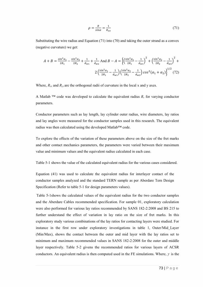
73 | P a g e

𝜌 =𝑅

𝑠𝑖𝑛𝛼=

1

𝑅𝑥𝑥 (71)

Substituting the wire radius and Equation (71) into (70) and taking the outer strand as a convex

(negative curvature) we get:

𝐴 + 𝐵 =𝑠𝑖𝑛2𝛼1

2𝑅1−

𝑠𝑖𝑛2𝛼2

2𝑅2+

1

𝑑𝑤1+

1

𝑑𝑤2 And 𝐵 − 𝐴 = {(

𝑠𝑖𝑛2𝛼1

2𝑅1−

1

𝑑𝑤1)2

+ (𝑠𝑖𝑛2𝛼2

2𝑅2−

1

𝑑𝑤2)2

+

2(𝑠𝑖𝑛2𝛼1

2𝑅1−

1

𝑑𝑤1) (

𝑠𝑖𝑛2𝛼2

2𝑅2−

1

𝑑𝑤2) 𝑐𝑜𝑠2(𝛼1 + 𝛼2)}

1/2

(72)

Where, Rxx and Ryy are the orthogonal radii of curvature in the local x and y axes.

A Matlab ™ code was developed to calculate the equivalent radius Rc for varying conductor

parameters.

Conductor parameters such as lay length, lay cylinder outer radius, wire diameters, lay ratios

and lay angles were measured for the conductor samples used in this research. The equivalent

radius was then calculated using the developed Matlab™ code.

To explore the effects of the variation of these parameters above on the size of the fret marks

and other contact mechanics parameters, the parameters were varied between their maximum

value and minimum values and the equivalent radius calculated in each case.

Table 5-1 shows the value of the calculated equivalent radius for the various cases considered.

Equation (41) was used to calculate the equivalent radius for interlayer contact of the

conductor samples analyzed and the standard TERN sample as per Aberdare Tern Design

Specification (Refer to table 5-1 for design parameters values).

Table 5-1shows the calculated values of the equivalent radius for the two conductor samples

and the Aberdare Cables recommended specification. For sample 01, exploratory calculation

were also performed for various lay ratios recommended by SANS 182-2:2008 and BS 215 to

further understand the effect of variation in lay ratio on the size of fret marks. In this

exploratory study various combinations of the lay ratios for contacting layers were studied. For

instance in the first row under exploratory investigations in table 1, Outer/Mid_Layer

(Min/Max), shows the contact between the outer and mid layer with the lay ratios set to

minimum and maximum recommended values in SANS 182-2:2008 for the outer and middle

layer respectively. Table 5-2 givens the recommended ratios for various layers of ACSR

conductors. An equivalent radius is then computed used in the FE simulations. Where, is the

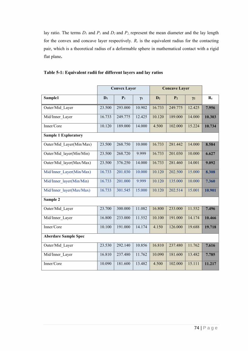
74 | P a g e

lay ratio. The terms D1 and P1 and D2 and P2, represent the mean diameter and the lay length

for the convex and concave layer respectively. Rc is the equivalent radius for the contacting

pair, which is a theoretical radius of a deformable sphere in mathematical contact with a rigid

flat plane.

Table 5-1: Equivalent radii for different layers and lay ratios

Convex Layer Concave Layer

Sample1 D1 P1 1 D2 P2 2 Rc

Outer/Mid_Layer 23.500 293.000 10.902 16.733 249.775 12.425 7.956

Mid/Inner_Layer 16.733 249.775 12.425 10.120 189.000 14.000 10.303

Inner/Core 10.120 189.000 14.000 4.500 102.000 15.224 10.734

Sample 1 Exploratory

Outer/Mid_Layer(Min/Max) 23.500 268.750 10.000 16.733 281.442 14.000 8.584

Outer/Mid_layer(Min/Min) 23.500 268.720 9.999 16.733 201.030 10.000 6.627

Outer/Mid_layer(Max/Max) 23.500 376.250 14.000 16.733 281.460 14.001 9.092

Mid/Inner_Layer(Min/Max) 16.733 201.030 10.000 10.120 202.500 15.000 8.308

Mid/Inner_layer(Min/Min) 16.733 201.000 9.999 10.120 135.000 10.000 7.360

Mid/Inner_layer(Max/Max) 16.733 301.545 15.000 10.120 202.514 15.001 10.901

Sample 2

Outer/Mid_Layer 23.700 300.000 11.082 16.800 233.000 11.552 7.496

Mid/Inner_Layer 16.800 233.000 11.552 10.100 191.000 14.174 10.466

Inner/Core 10.100 191.000 14.174 4.150 126.000 19.688 19.718

Aberdare Sample Spec

Outer/Mid_Layer 23.530 292.140 10.856 16.810 237.480 11.762 7.616

Mid/Inner_Layer 16.810 237.480 11.762 10.090 181.600 13.482 7.785

Inner/Core 10.090 181.600 13.482 4.500 102.000 15.111 11.217

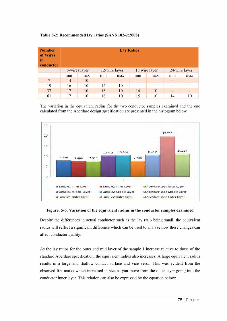
75 | P a g e

Table 5-2: Recommended lay ratios (SANS 182-2:2008) Number of Wires in conductor

Lay Ratios

6-wires layer 12-wire layer 18 wire layer 24-wire layer min max min max min max min max

7 14 10 - - - - - - 19 16 10 14 10 - - - - 37 17 10 16 10 14 10 - - 61 17 10 16 10 15 10 14 10

The variation in the equivalent radius for the two conductor samples examined and the one calculated from the Aberdare design specification are presented in the histogram below.

Figure: 5-6: Variation of the equivalent radius in the conductor samples examined

Despite the differences in actual conductor such as the lay ratio being small, the equivalent

radius will reflect a significant difference which can be used to analyze how these changes can

affect conductor quality.

As the lay ratios for the outer and mid layer of the sample 1 increase relative to those of the

standard Aberdare specification, the equivalent radius also increases. A large equivalent radius

results in a large and shallow contact surface and vice versa. This was evident from the

observed fret marks which increased in size as you move from the outer layer going into the

conductor inner layer. This relation can also be expressed by the equation below:

76 | P a g e

𝑡𝑎𝑛𝛼 = 𝜋 [1

𝛾−

2𝑅𝑤

𝑃]

−𝜋

2< 𝛼 <

𝜋

2 (73)

From Equation (73) as the lay ratio increases, the lay angle reduces hence increasing the

contact surface. Figure 8 shows the sizes for fret marks in different layers of the conductor.

From Equation (73) and the table we can conclude that winding conductor layers such that

there lay ratios are close to each other and both closer to the recommended maximum lay ratio

with result in a high value of the equivalent radius. Winding the same layers with lay ratios

close together but closer the minimum recommended lay ratio with will result in a smaller

equivalent radius.

(a) (b)

Figure 5-7: (a) Large and shallow mark for inner layer (b) Relatively smaller and deeper Fret mark for mid Layer

5.2.3 Finite Element Analysis (FEA)

The equivalent sphere of radius Rc was used for modeling in MSC Marc Mentat. A hemisphere

was modeled as being in mathematical contact with a rigid flat plane. Both linear elastic and

nonlinear analysis are presented. The quadrilateral element type 11 was used with large strain

in plain strain and Von Mises failure criterion. For the nonlinear simulation the actual stress

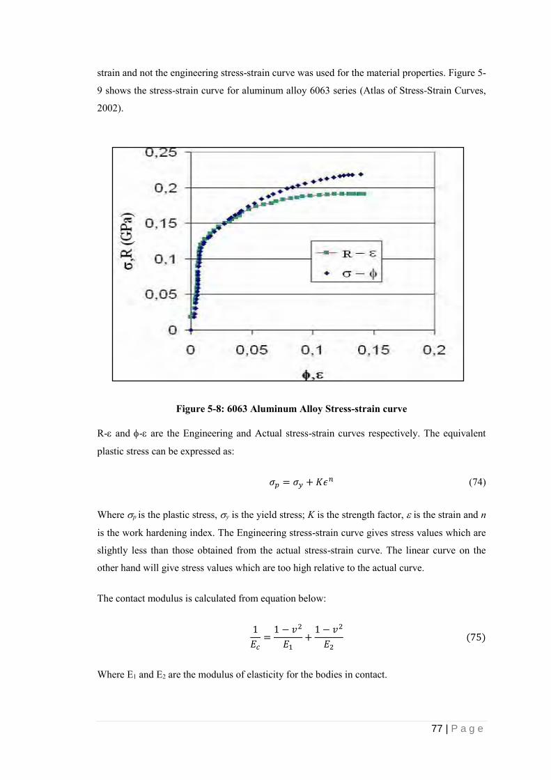
77 | P a g e

strain and not the engineering stress-strain curve was used for the material properties. Figure 5-

9 shows the stress-strain curve for aluminum alloy 6063 series (Atlas of Stress-Strain Curves,

2002).

Figure 5-8: 6063 Aluminum Alloy Stress-strain curve

R- and - are the Engineering and Actual stress-strain curves respectively. The equivalent

plastic stress can be expressed as:

𝜎𝑝 = 𝜎𝑦 + 𝐾𝜖𝑛 (74)

Where p is the plastic stress, y is the yield stress; K is the strength factor, is the strain and n

is the work hardening index. The Engineering stress-strain curve gives stress values which are

slightly less than those obtained from the actual stress-strain curve. The linear curve on the

other hand will give stress values which are too high relative to the actual curve.

The contact modulus is calculated from equation below:

1

𝐸𝑐=

1 − 𝑣2

𝐸1+

1 − 𝑣2

𝐸2 (75)

Where E1 and E2 are the modulus of elasticity for the bodies in contact.

78 | P a g e

When E1 is equal to E2 we get:

𝐸𝑐 =𝐸

2(1−𝑣2) (76)

Ec is the Contact modulus, E is the Modulus of Elasticity for Aluminum (69GPa) and v is the

Poisson’s ratio (0.31).With these values, a best fitting curve was fitted in equation (74) and

plotted in MSC Marc Mentat as shown in figure 5-10. The best fitting equation was expressed

as:

𝜎 =35(1 + 8.543휀0.044)𝑁

𝑚𝑚2 (78)

The hemisphere used in the contact modelling was given the load boundary conditions shown

in figure 5-9. The hemisphere was constrained by a fixed point on its top most point. The

hemisphere was subjected to a ramping load imposed by moving flat plane. The displacement

of the flat plane was set equal to the maximum interference observed in the outer and middle

layer contacting pair.

A job was created for large strain analysis. Figure 5-10 shows the job set-up.

Figure 5-9: Material properties in MSC Marc

79 | P a g e

Figure 5-10: Boundary Conditions (BCs)

(a) Job set-up

80 | P a g e

(b)

Figure 5-11: Successful completion of a job

The results from the post processing are shown in figure 5-13 (a) to (c).

(a) Equivalent Von Mises stress

81 | P a g e

(b) Displacement

(c) Hoop stress

Figure: 5-12: Results from the simulations

The results of the simulations are summarized in the tables below. The simulations were

carried out in 50 steps for the loading and 20 steps for the unloading. The tables only show the

50 loading steps.

82 | P a g e

Table 5-3: Simulation results for sphere of equivalent radius of 7.956mm

Increment Normal Contact

force(N)

Stress(MPa) Plastic strain

1 28.37 42.25 1.297E-3

2 42.01 54.00 4.33E-3

3 49.95 62.05 7.793E-3

4 55.61 68.3 1.152E-2

5 60.13 73.52 1.535E-2

6 63.95 73.52 1.535E-2

7 67.28 82.07 2.321E-2

8 70.25 85.72 2.72E-2

9 72.95 89.07 3.123E-2

10 75.43 92.18 3.527E-2

11 77.73 95.09 3.935E-2

12 79.87 97.38 4.344E-2

13 81.89 100.4 4.755E-2

14 83.79 102.9 5.169E-2

15 85.59 105.2 5.584E-2

16 87.3 107.5 6.002E-2

17 88.94 109.7 6.421E-2

18 90.21 112.6 7.015E-2

19 90.49 116.4 7.833E-2

20 90.75 120.0 8.658E-2

21 90.98 123.5 9.49E-2

22 91.18 126.8 1.033E-1

23 91.36 129.9 1.118E-1

24 91.52 132.9 1.203E-1

25 91.66 135.8 1.29E-1

26 91.79 138.7 1.377E-1

27 91.90 141.4 1.464E-1

28 92.0 144.1 1.553E-1

29 92.02 146.7 1.642E-1

30 92.17 149.2 1.733E-1

31 92.23 151.7 1.826E-1

32 92.29 154.1 1.92E-1

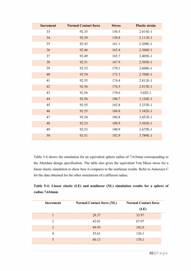
83 | P a g e

Increment Normal Contact force Stress Plastic strain

33 92.35 156.5 2.015E-1

34 92.39 158.8 2.111E-1

35 92.43 161.1 2.208E-1

36 92.46 163.4 2.306E-1

37 92.49 165.7 2.405E-1

38 92.51 167.9 2.505E-1

39 92.53 170.1 2.606E-1

40 92.54 172.3 2.708E-1

41 92.55 174.4 2.811E-1

42 92.56 176.5 2.915E-1

43 92.56 178.6 3.02E-1

44 92.56 180.7 3.126E-1

45 92.55 182.8 3.233E-1

46 92.55 184.8 3.342E-1

47 92.54 186.8 3.451E-1

48 92.53 188.9 3.562E-1

49 92.53 190.9 3.675E-1

50 92.51 192.9 3.789E-1

Table 5-4 shows the simulation for an equivalent sphere radius of 7.616mm corresponding to

the Aberdare design specification. The table also gives the equivalent Von Mises stress for a

linear elastic simulation to show how it compares to the nonlinear results. Refer to Annexure C

for the data obtained for the other simulations of a different radius.

Table 5-4: Linear elastic (LE) and nonlinear (NL) simulation results for a sphere of

radius 7.616mm

Increment Normal Contact force (NL) Normal Contact force

(LE)

1 28.37 33.97

2 42.01 67.97

3 49.95 102.0

4 55.61 136.1

5 60.13 170.1

84 | P a g e

Increment Normal Contact force (NL) Normal Contact force

(LE)

6 63.95 204.3

7 67.28 238.4

8 70.25 272.6

9 72.95 306.8

10 75.43 341.0

11 77.73 375.3

12 79.87 409.6

13 81.89 443.9

14 83.79 478.2

15 85.59 512.6

16 87.3 547

17 88.94 581.4

18 90.21 615.9

19 90.49 650.4

20 90.75 684.9

21 90.98 719.4

22 91.18 754

23 91.36 788.6

24 91.52 823.2

25 91.66 857.8

26 91.79 892.5

27 91.90 927.2

28 92.0 961.9

29 92.09 996.7

30 92.17 1031

31 92.23 1066

32 92.29 1083

33 92.35 1098

34 92.39 1113

35 92.43 1128

36 92.46 1143

37 92.49 1158

38 92.51 1174

39 92.53 1189

85 | P a g e

Increment Normal Contact force (NL) Normal Contact force

(LE)

40 92.54 1204

41 92.55 1219

42 92.56 1234

43 92.56 1249

44 92.56 1264

45 92.55 1280

46 92.55 1295

47 92.54 1310

48 92.53 1325

49 92.53 1340

50 92.51 1356

Notice the large difference in the contact force between the linear elastic and the nonlinear

simulation results. This difference can also be seen from figure 5-14. The deformation can be

seen to be more in the nonlinear simulation (a). The linear elastic simulation used 50

increments for the simulation and not the 70 used for the nonlinear. This is because for the

linear elastic the deformation can only be seen as the load is applied, which is the first 50

increments and will regain its original shape when the load is removed in the last 20 steps

(a) Nonlinear simulation result

86 | P a g e

(b) Linear elastic simulation result

Figure 5-13: (a) Nonlinear result (b) linear Elastic result

The relationship between the equivalent sphere radius and the Von Mises stress, plastic strain,

fret mark dimensions and the normal contact force for the nonlinear simulation are explained

below.

5.2.3.1 Total equivalent plastic strain

A plot of the equivalent radius versus the total equivalent plastic strain is shown in figure 5-14.

There is very strong linear correlation between the equivalent radius and the plastic strain with

a correlation constant of 0.915. The plastic strain decreases linearly with the increase in the

equivalent radius. This results implies very deep fret marks for a lower value of the equivalent

radius. This supports the observation presented above.

87 | P a g e

Figure 5-14: Equivalent radius vs Total Equivalent plastic strain

5.2.3.2 Von Mises stress

The Von Mises stress shows a strong linear correlation with the equivalent radius. It decreases

linearly with an increase in the equivalent radius. The correlation constant is 0.926. This

implies that for a smaller equivalent radius, there is more stress at the contact surfaces which

will result in high plastic strain and hence more deformation. For the simulated outer layer,

there exist a theoretical equivalent radius of 26.74mm which will result in zero contact stress

and hence zero plastic strain. Winding the conductor such that the equivalent radius is closer to

this value will result in better conductor quality. Fig. 5-15 shows how the Von Mises stress

varies with the equivalent radius.

Figure 5-15: Equivalent radius vs Equivalent von mises stress

0,25

0,3

0,35

0,4

0,45

0,5

6 7 8 9 10 11

Equ

ival

en

t P

last

ic s

trai

n

Equivalent Radius(mm)

Equivalent Radii vs Equivalent Plastic Strain

Equivalent Plastic Strain

Linear (Equivalent PlasticStrain)

y = -10,297x + 275,35R² = 0,8575

150

160

170

180

190

200

210

6 7 8 9 10 11

Equ

ival

en

t V

on

Mis

es

Stre

ss(M

Pa)

Equivalent Radius(mm)

Equivalent Radii vs Equivalent Von Mises Stress

Von Mises Stress

Linear (Von Mises Stress)

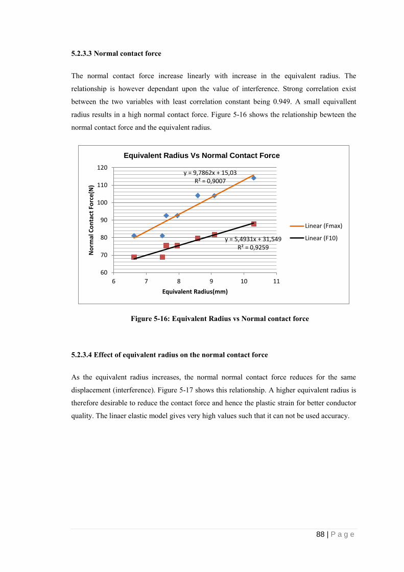
88 | P a g e

5.2.3.3 Normal contact force

The normal contact force increase linearly with increase in the equivalent radius. The

relationship is however dependant upon the value of interference. Strong correlation exist

between the two variables with least correlation constant being 0.949. A small equivallent

radius results in a high normal contact force. Figure 5-16 shows the relationship bewteen the

normal contact force and the equivalent radius.

Figure 5-16: Equivalent Radius vs Normal contact force

5.2.3.4 Effect of equivalent radius on the normal contact force

As the equivalent radius increases, the normal normal contact force reduces for the same

displacement (interference). Figure 5-17 shows this relationship. A higher equivalent radius is

therefore desirable to reduce the contact force and hence the plastic strain for better conductor

quality. The linaer elastic model gives very high values such that it can not be used accuracy.

y = 9,7862x + 15,03R² = 0,9007

y = 5,4931x + 31,549R² = 0,9259

60

70

80

90

100

110

120

6 7 8 9 10 11

No

rmal

Co

nta

ct F

orc

e(N

)

Equivalent Radius(mm)

Equivalent Radius Vs Normal Contact Force

Linear (Fmax)

Linear (F10)

89 | P a g e

Figure 5-17: Inference per layer vs. Normal contact force

5.2.3.5 Fret mark dimensions versus equivalent radius

The relationship between the fret mark and the equivalent radius has a parabolic appearance

with a correlation constant of 0.947. This relationship suggests that there exist a maximum fret

mark length which can be obtained for a given tension for a particular set-up. Refer to figure 5-

19. A straight line can also be fitted on this data although it gives a weaker correlation.

Figure 5-18: Equivalent Radius vs. Length of fret mark

0

20

40

60

80

100

120

0 0,1 0,2 0,3 0,4 0,5

No

rmal

Co

nta

ct F

orc

e (

N)

Interference

Interference Vs Normal Force

6.627mm

7.616mm

8.584mm

7.616mm(Linear Elastic)

1900

2000

2100

2200

2300

2400

2500

2600

2700

7 8 9 10 11

Len

gth

, Bo

tto

m f

ret

laye

r Fr

et

mar

ks(m

m)

Equivalent Contact Radius

Relative Radii Vs Length of Fret Mark

Equivalent Radius

90 | P a g e

The depth of the fret marks decreased as the equivalent radius increased. This is depicted in

figure 5-20. If the two outlying points are neglected based on the assumption that there was an

error in measurement, a strong linear correlation is observed between the equivalent radius and

the depth of the fret marks with a correlation constant of 0.9996. From this linear regression, a

hypothetical equivalent radius of 12.772mm would result in zero indentation depth at the

winding tension used for this conductor sample. If however the points are taken into account,

the data shows a large scatter and no simple relationship can be established.

Figure 5-19: Equivalent Radius versus fret mark depth

From the results, it can be seen that the outer layer will have the deepest marks as it has the

smallest equivalent radius. The equivalent radius is directly proportional to the difference

between the curvatures (reciprocal of equivalent radii of curvature) of the contacting surfaces.

Because the lay angles are generally small, the size of the curvature can be said to be inversely

proportional to the radius of the helix about the conductor axis as given in Eq. (9). Therefore

the outer layer having the largest value or the helix radius will have the smallest curvature and

hence would give the smallest equivalent radii. The middle layer is more susceptible to failure

as it has mark on both sides. On average the middle layer has total depth in excess of

420microns, which is the sum of depths of the marks on either side (top and bottom) for the

samples analyzed. This reduces the effective length of crack propagation by 12%. This implies

that the crack has a shorter cross section of the strand to propagate before it reaches the critical

length.

150

200

250

300

350

400

450

7 7,5 8 8,5 9 9,5 10 10,5 11

Inte

rfe

ren

ce p

er

laye

r to

laye

r co

nta

ct(m

icro

ns)

Equivalent Contact Radii

Equivalent Contact Radii vsTotal Depth

91 | P a g e

5.3 Inner conductor contact model

The normal contact force from the FE model was used to calculate the tension applied to the

conductor wire to obtain the observed average interference. The inner conductor contact

mechanics is model as massless strands connected by springs. Figure 5-21 shows the model

used to calculate the tension. In figure 5-21 (a), K is the vertical component of the radial

contact stiffness k. The forces pushing each layer downwards are designated as F1, F2, F3, F4

and the corresponding displacement as X1, X2, X3 and X4. Using the finite element method, the

stiffness and the forces causing the displacement can be expressed in matrix form:

𝐹 = 𝐾𝑋 (79)

Where F is the force, K is the stiffness and X is the displacement. In terms of the vertical

stiffness, K, the matrix equation is:

[

𝐾1 −𝐾1 0 0−𝐾1 𝐾1 + 𝐾2 −𝐾2 0

0 −𝐾2 𝐾2 + 𝐾3 −𝐾3

0 0 −𝐾3 𝐾3

] [

𝑋1

𝑋2

𝑋3

𝑋4

] = [

𝐹1

𝐹2

𝐹3

𝐹4

] (80)

At Equilibrium X4 is zero. The interference per layer is given by the difference in

displacements i.e. for a1 (outer vs. middle layer); 𝑎1 = 𝑋1 − 𝑋2

In figure 5-21(b) the symbols; S1, S2 and S3 denote the strands of the outer layer that are

contacting the layer beneath. The radial contact force and displacement are resolved and their

vertical components expressed as an equivalent stiffness.

Figure 5-21 shows the outer layer strands contacting the layer underneath. i is the angle

between the strands in the layer and for compact packing is given by ;

∅𝑖 = 2𝜋

𝑛𝑖 (81)

Where ni is the number of strands in the layer, i is layer number with i=1 being the outer layer.

Resolving all the radial stiffness in the vertical direction, we can obtain the following value of

total vertical stiffness for a finite length of the conductor, for K1;

𝐾1𝑡𝑜𝑡𝑎𝑙 = 𝐾1 + 𝐾1𝑐𝑜𝑠𝑛∅1 + 𝐾2𝑐𝑜𝑠∅2 + ⋯+ 𝐾𝑛𝑖𝑐𝑜𝑠∅𝑛𝑖 (82)

92 | P a g e

Where K1total is the total vertical stiffness in the vertical direction for a finite length of the

conductor. Equation (47) can be expressed in compact form as:

𝐾1𝑡𝑜𝑡𝑎𝑙 = 𝐾1 ∑𝑐𝑜𝑠𝑛𝑖∅𝑛𝑖

𝑛𝑖

0

(83)

All the three radial stiffness can be expressed in a similar form and substituted in equation (45)

to give:

(

𝐹1

𝐹2

𝐹3

𝐹4

)

=

[

𝐾1 ∑𝑐𝑜𝑠𝑛∅1

𝑛𝑖1

0

−𝐾1 ∑𝑐𝑜𝑠𝑛∅1

𝑛𝑖1

0

0 0

−𝐾1 ∑𝑐𝑜𝑠𝑛∅1

𝑛𝑖1

0

𝐾1 ∑𝑐𝑜𝑠𝑛∅1

𝑛𝑖1

0

+ 𝐾2 ∑𝑐𝑜𝑠𝑛∅2

𝑛𝑖2

0

−𝐾2 ∑𝑐𝑜𝑠𝑛∅2

𝑛𝑖2

0

0

0 −𝐾2 ∑𝑐𝑜𝑠𝑛∅2

𝑛𝑖2

0

𝐾2 ∑𝑐𝑜𝑠𝑛∅2

𝑛𝑖2

0

+ 𝐾3 ∑𝑐𝑜𝑠𝑛∅3

𝑛𝑖3

0

0

0 0 −𝐾3 ∑𝑐𝑜𝑠𝑛∅3

𝑛𝑖3

0

𝐾3 ∑𝑐𝑜𝑠𝑛∅3

𝑛𝑖3

0 ]

[

𝑋1

𝑋2

𝑋3

𝑋4

]

(a) (b)

Figure 5-20: Inner Conductor contact mechanics model

93 | P a g e

From this matrix equation:

𝐹1 = (𝑋1 − 𝑋2)𝐾1 ∑ 𝑐𝑜𝑠𝑛∅1𝑛𝑖10 (84)

𝐹2 = 𝐾1 ∑𝑐𝑜𝑠∅2

𝑛𝑖3

0

(𝑋3 − 𝑋2) + 𝐾3𝑋3 ∑𝑐𝑜𝑠∅3

𝑛𝑖3

0

(85)

𝐾4𝑋3 ∑𝑐𝑜𝑠∅3

𝑛𝑖3

0

= 𝐹4 (86)

If we consider a finite length of the conductor, L, the ratio of the number of wires in each layer

in this length is:

𝑠𝑖𝑛𝛼1

𝑑1:𝑠𝑖𝑛𝛼2

𝑑2:𝑠𝑖𝑛𝛼3

𝑑3

For nx wire in the outer layer, the contact force per fret mark (F1c) is given by;

𝐹1𝑐 = (𝐹1) (𝑑2𝑠𝑖𝑛𝛼1

𝑛𝑥𝑑1𝑠𝑖𝑛𝛼2) With ni1= nx (87)

F1 is the normal contact force per fret mark obtained from the FEA simulations.

From the inner conductor contact model by Hruska, 1953 the Tension conductor is given by:

𝑇 =𝑓𝑖(𝐴𝐸)

𝐴𝑖𝐸𝑖𝑐𝑜𝑠2𝛼𝑖, 𝑓𝑖 =

𝐹1𝑐

sin𝛼 and 𝐴𝐸(𝑎𝑥𝑖𝑎𝑙 𝑆𝑡𝑖𝑓𝑓𝑛𝑒𝑠𝑠) = 𝐸𝑐𝐴𝑐 + ∑ 𝑛𝑖𝐴𝑖𝐸𝑖𝑐𝑜𝑠3𝛼𝑖

𝑚1 (89)

Where m is the layer number, A is cross section area and E is modulus of elasticity. To

calculate the force per aluminum wire one needs to find the tension in the core alone given by:

𝐹𝑐 =𝐴𝑐𝐸𝑐

(𝐴𝐸)𝑇 (90)

Where; Ac and Ec are the cross section area and the Young Modulus of the core respectively.

94 | P a g e

6. Fatigue crack propagation

Determination of the fatigue crack propagation curve is an essential part of the fracture

mechanics design approach. Residual strength calculations do have shortcomings, but the

prediction of crack propagation is even less accurate, despite the vast amount of research

conducted in this subject (Broek D., 1986). For compound structures such as the transmission

line conductors very little data is available for the prediction of the crack growth. This chapter

is therefore dedicated to modelling of the fatigue data using Linear Elastic Fracture Mechanics

(LEFM).

6.1 Crack growth and the stress intensity factor

In the elastic case the stress intensity factor is sufficient parameter to describe the whole stress

field at the tip of the crack. When the size of the plastic zone is small compared to the crack

length, the stress intensity factor is a good indication of the stress environment of the crack tip.

If two different cracks have the same stress environment, they will behave in the same manner

and show equal crack growth rate. The rate of fatigue crack growth is then governed by the

stress intensity factor. This can be expressed mathematically as shown in equation (91).

𝑑𝑎

𝑑𝑁= 𝑓(∆𝐾) = 𝑓{(𝑆𝑚𝑎𝑥 − 𝑆𝑚𝑖𝑛)√𝜋𝑎 (91)

Where:

∆𝐾 is the Stress intensity factor range

Smin and Smax are the minimum and maximum stresses in the cycle

a is the crack length

N is the number of fatigue cycles

Paris, Gomez and Anderson where the first to point this out (Broek D, 1986). Equation (91) is

sometimes expressed as a simple power function:

𝑑𝑎

𝑑𝑁= 𝐶(∆𝐾)𝑛 (92)

In this equation, C and n are supposed to be material constants. A double logarithmic plot of 𝑑𝑎

𝑑𝑁 versus ∆𝐾 would then be a straight line. In this law.

95 | P a g e

Equation (92) is a case of LEFM and does not fully represent reality. Actual fatigue data falls

on an S-Shaped curve which can be broken down into three regions.

o Region 1-Non continuum behaviour

In this region, the behaviour of the crack is largely influenced by the following:

I. Microstructure

II. Mean stress

III. Environment

o Region 2-Continuum behaviour

This region is the linear part of the double logarithmic plot the power law (Paris law).

For a failed metallic material in this region, there are usually striations on the failed

surface. This region is characterized by the following:

I. Small to large influence of the microstructure depending on the material

II. Large influence of a certain combinations of the environment, mean stress,

and frequency.

o Region 3:- Static mode behaviour

This is the unpredictable region in the curve and it’s associated with features such as

cleavage, intergranular and dimples. This region has the following characteristics:

I. Large influence of the microstructure, mean stress and thickness

II. Little influence of the environment

In region 1, there exist a threshold stress intensity factor ∆𝐾𝑇𝐻 at which cracks propagate at a

very slow rate or do not propagate at all. Above this value of the stress intensity factor, the

crack propagates relatively rapidly with increasing stress intensity factor range.

In region 2 the crack growth rate, da/dn is a power function of ∆𝐾. Finally in region 3, the

crack growth curve raises rises to an asymptote where maximum stress intensity factor, Kmax

becomes equal to the critical stress intensity factor Kc, the fracture toughness of the material.

Many equations have been proposed to try and describe the crack growth curve. The mostly

widely known is the Paris equation:

𝑑𝑎

𝑑𝑁= 𝐶(∆𝐾)𝑚 (93)

Forman proposed the following well known improved equation:

𝑑𝑎

𝑑𝑛=

𝐶(∆𝐾)𝑚

(1 − 𝑅)𝐾𝑐 − ∆𝐾 (94)

96 | P a g e

R is the ratio of the maximum stress to the minimum stress.

Many variations of the Paris equation, exist but the analysis used in this research was based on

the Paris law itself.

6.2 Modelling of the fatigue data

The modelling of the fatigue data was based on the assumption of centre crack on an infinite

specimen as most of the cracks were observed to be transverse to the direction of the fret

marks measured on the major axis. In this case the stress intensity factor range can be

calculated using as:

∆𝐾 = ∆𝜎√𝜋𝑎√𝐷

𝜋𝑎tan (

𝜋𝑎

𝐷) (95)

Where:

∆𝜎 is the stress range

D is the diameter of the strand

a is the crack length.

This equation holds for the condition:

𝑎

𝐷< 0.25

Using the fatigue crack data from tables 4-3 and 4-4 respectively, the stress intensity factor

was calculated and used in the modelling of the fatigue data. Table 6-1 shows the values of the

calculated stress intensity factors.

97 | P a g e

Table 6-1: Stress Intensity factors for sample 1

From the table log K is the logarithm of the stress intensity factor range and the last column

shows the logarithm of the rate of crack growth. The actual stresses where calculated using the

assumption of bending solid bar. The Euler-Bernoulli equation was used to approximate the

stresses at various interfaces using the measured stresses on the surfaces.

𝑀 =𝜎𝐼

𝑦 (96)

Where:

M is the moment

I is the second moment of area

𝜎 is the stress

y is the distance from the centre of the conductor core to the point where the stress has to be

measured.

Using the Paris law, a double logarithmic plot of the data was done and is shown in figure 6-1

below.

The double logarithm plot will give a straight line of the form:

log𝑑𝑎

𝑑𝑛= log𝐶 + 𝑚 log∆𝐾 (97)

A straight line whose gradient is m and intercept is log C can be fitted in the fatigue data.

Location (Linear distance)-mm

Layer Crack length-microns

Strain-microstrains

Stress-MPa Actual Stress Delta K logK lg(da/dn)

15 Outer Layer 485,3 680 47,60 35,7 1444,606986 3,159749711 -11,0129690 Midlayer 167,3 158 10,90 8,175 188,1912549 2,274599438 -11,4754745 Mid-layer 84,33 895 61,76 46,31625 754,6976203 2,877772981 -11,772988

45 Mid-layer 173,6 150 10,35 7,7625 182,0858103 2,260276103 -11,4594260 Mid-layer 222,5 10 0,69 0,5175 13,78180958 1,139306245 -11,3516460 Mid-layer 102,9 10 0,69 0,5175 9,319333019 0,969384831 -11,68655585 Mid-layer 176,8 115 7,94 5,95125 140,9029112 2,148919966 -11,45148880 Mid-layer 115,1 75 5,18 3,88125 73,95085918 1,868943224 -11,63789590 Mid-layer 81,19 165 11,39 8,53875 136,5090712 2,135161512 -11,789467

98 | P a g e

Figure 6-1: Log-log plot of fatigue data for sample 1

A straight line of best fit was then fitted into this data and is shown in figure 6-2.

Figure 6-2: Best fit line

-11,9

-11,8

-11,7

-11,6

-11,5

-11,4

-11,3

-11,2

-11,1

-11

-10,9

0 0,5 1 1,5 2 2,5 3 3,5LO

G(R

ATE

OF

CR

AC

K G

RO

WTH

)

LOG(DELTA K)

Lg(ΔK) vs. lg(da/dn)

y = 0,3058x - 12,1R² = 0,8306

-11,9

-11,8

-11,7

-11,6

-11,5

-11,4

-11,3

-11,2

-11,1

-11

-10,9

0 0,5 1 1,5 2 2,5 3 3,5

LOG

OF

CR

AC

K G

RO

WTH

RA

TE

LOG DELTA K

Sample1

99 | P a g e

From this best fit line fitted with a correlation constant of 0.91, a gradient of 0.3058 and

intercept of -12.1 were found. From these value the following values of C and m were

calculated.

𝐶 = 7.943 × 10−13 𝑎𝑛𝑑 𝑚 = 0.3058

A crack growth law of the following form was established;

𝑑𝑛

𝑑𝑎= 7.943 × 10−13(∆𝐾)0.3058 (98)

The values of C and m in this case are not material constants but rather structure constants for

this set-up. Table 6-2 shows a comparison between the cracks calculated from this law and the

actual crack size. The average value of the variance is 11.766%. The same procedure described

here was applied to data for sample 1 and a crack growth law with 𝐶 = 4.1 × 10−14 𝑎𝑛𝑑 𝑚 =

0.7466. The variance for this law averaged at -17.969%.

Table 6-2: Comparison of the calculated crack length to the actual length

Crack length (Calculated ) Crack length(Actual) Variance

375,57 485,30 -22,61 200,15 167,30 19,63 307,33 84,33 264,44 198,12 173,60 14,12 89,28 222,50 -59,87 79,12 102,90 -23,11 183,04 176,80 3,53 150,00 115,10 30,32 181,26 81,19 123,25 25,16 61,59 -59,15 21,10 44,87 -52,96 9,61 266,90 -96,40

Average 11,7662

6.3 Equivalent Initial Flaw Size (EIFS)

The Equivalent Initial Flaw Size (EIFS) is the size of the initial flaw that under-static cyclic

loading would result in a prescribed endurance. The calculation of the value of the EIFS was

based on the established crack growth laws and back extrapolation of the fatigue data.

100 | P a g e

Integration of the Paris law given by equation (93) for a centre crack on an infinite plate will

give the following result:

𝑎𝑓

2−𝑚2 + 𝑎𝑜

2−𝑚2 = (

𝑚 − 2

2)

𝐶

√𝜋3 . 𝑁 (99)

Where N is the number of fatigue cycles.

Where:

𝑎𝑓 is the final crack length after N cycles

𝑎𝑜 is the EIFS

For sample 1 with a maximum final crack length of 266.9 microns, the EIFS was found to be

266.899 microns. For the second sample the EIFS was found to be 270.40 microns.

Assuming a linear relationship between the EISF and the actual average fret marks

dimensions, the following dimensions were obtained for an EIFS of size zero;

o Fret mark length of 2457.538 microns

o Fret mark width of 407.98 microns

o Fret mark Depth of 217.413 microns

These dimensions can be taken as the maximum allowable initial flaw size for the conductor at

manufacturing.

101 | P a g e

7. Conclusion

The surface quality of the manufactured TERN ACSR conductor has been studied and its

contact mechanics analysed. Both linear elastic and nonlinear finite element analysis has been

used to determine the normal contact force and hence the tension injected in the conductor

during manufacturing to result in this surface quality. From the conductor inner contact

mechanics model presented, it was shown that a tension of 4.4kN was used during the

manufacturing of the conductor. This tension resulted in an interference averaging about 432

microns in the outer layer.

The outer layer has the smallest equivalent radius and hence will have the deepest fret marks

as the depth is inversely proportional to the equivalent radius. These deep marks will result in a

higher stress concentration factor and hence earlier nucleation of cracks. For layers with large

equivalent radii and hence large fret marks, crack nucleation will be delayed but if the surface

becomes too large, multiple cracks might initiate and eventually merge to cause failure. Hence

the equivalent radius must not be too large even if a larger one would result in a lower stress

concentration.

The calculated tension of 4.4kN will require the bobbin braking system to be set at 12.83kg

(13) for a bobbin of 200mm flange size. From the results presented it is recommended that

the winding set-up is such that the lay ratios for the contacting layers are relatively closer to

each and closer to the maximum recommended lay for those layers for improved strand

surface quality. Although a maximum equivalent radii to result in theoretically no fret marks

on the strand surfaces has being given, it would be practically too challenging to achieve it.

The calculated radius of 12.77mm can be achieved by setting the outer layer lay ratio to 14

which is the maximum permissible but this will require the mid-layer ratio to be set to over 20.

This is would be way above the recommended maximum ratio of 15 for this layer and hence

the conductor would not be compliant to the current manufacturing standards.

The analyses from the Energy dispersive Spectroscopy (EDS) showed that oxygen is present

before and after the fatigue testing indicating that fretting was occurring throughout the life of

the conductor samples. The presence of a high percentage of zinc (maximum of 13.45%) for an

untested sample and 0% after testing indicates that there might be some of form of loss of the

galvanization on the core wires.

The fractographic analysis showed that by 40 million cycles of fatigue testing, cracks had

already evolved and by 50 million cycles they had grown to a maximum size of 485.3 microns.

102 | P a g e

From the established fatigue crack propagation models, the equivalent initial flaw size of

454.49 microns and 270.43 microns for sample one and two were calculated respectively.

Using the EISF and assuming a linear back extrapolation, the maximum allowable surface

defect of the conductor was estimated to be 2457.54 microns, 407.98 microns and

217.41microns for the length, width and depth of the fret marks respectively.

103 | P a g e

8. References

1. Shigley,J., and Bundynas, R., (2008). Mechanical Engineering Design. Tata McGraw-

Hill, New Delhi.

2. Jansen, M., Zuidema, J., and Wanhill, R.,(2002). Fracture Mechanics, 2nd Edition,

Spons Press, London.

3. Mathur, D., (1981).Mechanics. S. Chand and Company limited, New Delhi.

4. Guirgutiu, V.,(2008). Structural Health Monitoring with Piezoelectric Wafer Active

Sensors. Elsevier, New York.

5. T.L. Anderson, T.L,. (1991). Fracture Mechanics, Fundamentals and Applications.

CRC Press, Florida.

6. S. Rao, S.,(2004). Mechanical Vibrations, 4th Edition. Pearson Education, Miami.

7. Benham, P.P,. and R.J. Crawford, R.J,.(1987).Mechanics of Engineering Materials.

Longman Scientific & Technical, New York.

8. Timoshenko, S., and J. Gere, J,.(1998). Mechanicals of Materials. Stanley Thornes

Ltd, Cheltenham.

9. Broek, D,.(1986). Elementary Engineering Fracture Mechanics, 4th Edition, Kluwer

Academic Publishers, Dordrecht.

10. Bougue, M,.(2009).High Voltage overhead Power Lines, Theoretical Calculations and

formulae for conductor installations. Crown Publications cc, Johannesburg.

11. O’Connor, P.D,. and Kleyner, A,.(2012). Practical Reliability Engineering, 5th

Edition, Wiley, West Sussex.

12. Bisnatch, s,. et al (2006). The Fundamentals and Practice of Overhead Line

Maintenance. Crown Publishers cc, Johannesburg.

13. Kogut, L. and Etsion, I., 2002. Elastic-plastic contact analysis of a sphere and a rigid

flat. Journal of Applied Mechanics.

14. Sanders A.P. and Brannon R.M., 2011.Determining a surrogate contact pair in hertzian

contact problem. Journal of Tribology.

15. Vu-quoc, L., Zhang, X., and Lesburg, L. 2000. A Normal Force-Displacement Model

for Contacting Spheres Accounting for Plastic Deformation: Force Driven

Formulation. ASME J. Appl. Mech, 67, pp.363-371.

16. Antoine, J. F., Visa, C., Sauvey, C., and Abba, G. 2006.Approximate analytical Model

for Hertzian Elliptical Contact Problems. ASME J. Tribology.

17. Sanchez-Brea, L.M., Gomez-Pedrero, J.A., and Bernabeu, E. 1999. Measurement of

surface defects on thin steel wires by atomic force microscopy. Journal of Applied

Surface science.

104 | P a g e

18. Kogut, L. and Etsion, I. 2002. A Finite Element Based Elastic-Plastic Model for the

Contact of Rough surfaces. Tribology Transactions

19. Johnson, K. L., 1985. Contact Mechanics, First Ed, Cambridge University Press,

Cambridge.

20. Timoshenko, S.P., and Goodier, J. N. 1970.Theory of Elasticity. Second Ed, McGraw

Hill, New York)

21. Cardou, A. 2013. Stick-Slip Mechanical Models for Overhead Electrical Conductors in

Bending. Universite’ Laval, Quebec)

22. Hale, L. C. 1999. “Contact Mechanics, in “Principles and Techniques for designing

precision machines. “MIT PhD Thesis, pp. 417-426.

23. Rawlins, C.B. 2005. Analytical Elements of Overhead Conductor Fabrication. First

Ed. Fultus Corporation.

24. The Planning, Design and construction of Overhead Power Lines .2010. Eskom Power

series

25. Brandon, D. and Kaplan, D. W. 2008. Microstructural Characterization of Materials.

Second Ed. John Wiley & sons, Ltd, West Sussex)

26. Xie, J. 2011. Stereomicroscopy: 3D Imaging and the Third Dimension Measurement.

Application Note, Agilent Technologies.

27. EPRI AC Transmission Line Reference Book-200kV and Above.2006. 2nd Ed, the

Orange Book

28. https://en.wikipedia.org/wiki/K%C3%A1rm%C3%A1n_vortex_street

29. http://www.mscsoftware.com/product/marc

30. http://www.afgrow.net/applications/DTDHandbook/

31. http://www.mech.utah.edu/~me7960/lectures/Topic7-

ContactStressesAndDeformations.pdf

32. http://feaforall.com/2014/10/23/hertz-contact/

33. http://solareis.anl.gov/documents/docs/APT_61117_EVS_TM_08_4.pdf

34. https://www.jic.ac.uk/microscopy/intro_EM.html

35. https://books.google.co.za/books?id=NojlBwAAQBAJ&pg=PA106&lpg

36. http://www.microscopemaster.com/electron-microscope.html

37. http://www.mechanical.in/engineering-metrology-and-measurements-subject-notes/

38. http://www.nist.gov/calibrations/upload/89-4088.pdf

39. https://www.youtube.com/watch?v=oNqSzzycRhw

40. http://www.sciencedirect.com/science/article/pii/S0142112308001710

41. http://www.managementstudyguide.com/quality-control-techniques.htm

105 | P a g e

Annexure A Strands Tensile Tests Certificate

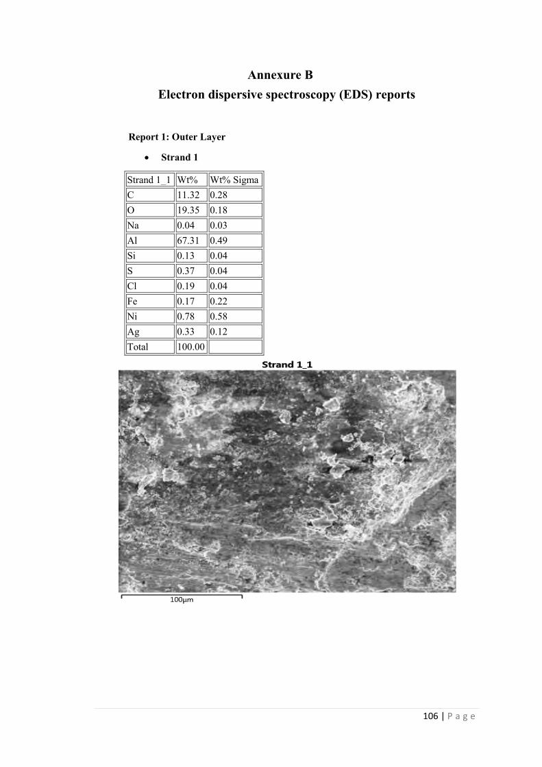
106 | P a g e

Annexure B Electron dispersive spectroscopy (EDS) reports

Report 1: Outer Layer

Strand 1

Strand 1_1 Wt% Wt% Sigma C 11.32 0.28 O 19.35 0.18 Na 0.04 0.03 Al 67.31 0.49 Si 0.13 0.04 S 0.37 0.04 Cl 0.19 0.04 Fe 0.17 0.22 Ni 0.78 0.58 Ag 0.33 0.12 Total 100.00

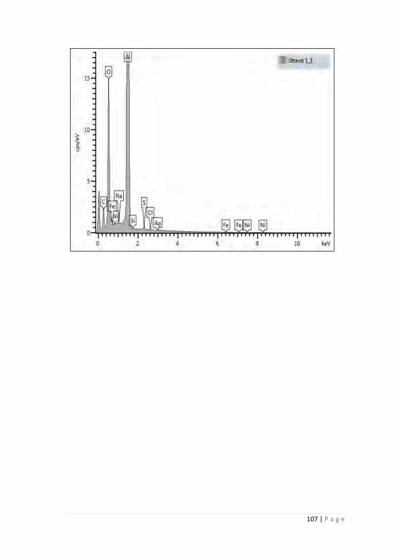
107 | P a g e

108 | P a g e

Report 2: Middle layer

Strand 1, point 1

Sample 2_1 Wt% Wt% Sigma C 0.00 0.00 O 10.23 0.22 Al 84.67 0.24 Si 3.75 0.06 Ar 0.08 0.05 K 0.23 0.03 Ca 0.09 0.02 Fe 0.49 0.04 Ag 0.47 0.12 Total 100.00

109 | P a g e

110 | P a g e

Strand 1, point 2

Sample 2_2 Wt% Wt%

Sigma C 0.00 0.00 O 8.33 0.23 Al 89.85 0.26 Si 0.66 0.04 Ar 0.00 0.00 K 0.06 0.03 Ca 0.17 0.03 Fe 0.40 0.05 Ag 0.53 0.13 Total 100.00

111 | P a g e

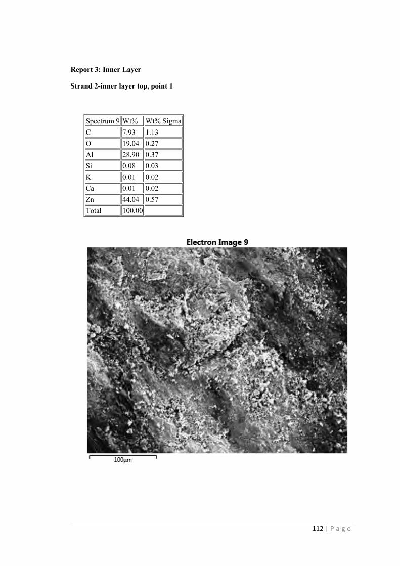
112 | P a g e

Report 3: Inner Layer

Strand 2-inner layer top, point 1

Spectrum 9 Wt% Wt% Sigma C 7.93 1.13 O 19.04 0.27 Al 28.90 0.37 Si 0.08 0.03 K 0.01 0.02 Ca 0.01 0.02 Zn 44.04 0.57 Total 100.00

113 | P a g e

114 | P a g e

Report 1: Inner Layer

strand1_top Wt% Wt% Sigma

C 9.56 0.80 O 15.48 0.21 Al 71.70 0.65 Si 2.76 0.06 K 0.11 0.03 Fe 0.40 0.05 Total 100.00

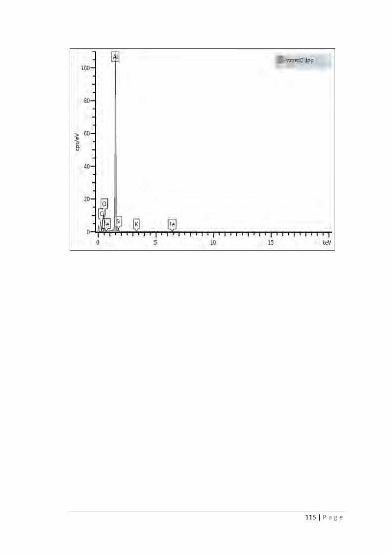
115 | P a g e

116 | P a g e

Report 2: Middle Layer

Spectrum 19 Wt% Wt%

Sigma O 17.37 0.17 Al 76.14 0.18 Si 5.72 0.08 Ar 0.12 0.03 K 0.15 0.03 Fe 0.50 0.05 Total 100.00

117 | P a g e

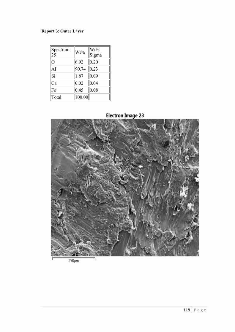
118 | P a g e

Report 3: Outer Layer

Spectrum 25 Wt% Wt%

Sigma O 6.92 0.20 Al 90.74 0.23 Si 1.87 0.09 Ca 0.02 0.04 Fe 0.45 0.08 Total 100.00

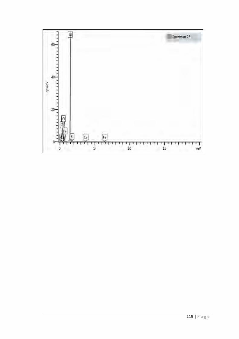
119 | P a g e

120 | P a g e

Annexure C

Simulation results for different equivalent radii

Table C1: Simulation results for sphere of equivalent radius of 8.584mm

Increment Normal Contact force Stress Plastic strain

1 24.72 38.18 6.805E-4

2 40.21 49.66 2.95E-3

3 49.87 57.58 5.728E-3

4 56.7 63.74 8.726E-3

5 62.04 68.86 1.19E-2

6 66.47 73.29 1.52E-2

7 70.3 77.23 1.856E-2

8 73.7 80.79 2.197E-2

9 76.76 84.06 2.542E-2

10 79.56 87.08 2.891E-2

11 82.15 89.91 3.242E-2

12 84.56 92.57 3.596E-2

13 86.82 95.08 3.951E-2

14 88.95 97.47 4.309E-2

15 90.96 99.75 4.669E-2

16 92.88 101.9 5.03E-2

17 94.7 104.0 5.393E-2

18 96.45 106.0 5.758E-2

19 98.12 108.0 6.125E-2

20 99.73 109.9 6.493E-2

21 100.7 113.1 7.149E-2

22 101.0 116.4 7.862E-2

23 101.3 119.5 8.582E-2

24 101.5 122.6 9.308E-2

25 101.8 125.5 1.004E-1

26 102.0 128.2 1.078E-1

27 102.2 130.9 1.152E-1

28 102.4 133.6 1.227E-1

121 | P a g e

Increment Normal Contact force Stress Plastic strain

29 102.5 136.1 1.303E-1

30 102.7 138.6 1.379E-1

31 102.8 141.0 1.456E-1

32 103.0 143.3 1.534E-1

33 103.1 145.6 1.612E-1

34 103.2 147.8 1.691E-1

35 103.3 150.0 1.771E-1

36 103.4 152.2 1.853E-1

37 103.5 154.3 1.935E-1

38 103.5 156.5 2.019E-1

39 103.6 158.5 2.109E-1

40 103.7 160.6 2.189E-1

41 103.7 162.6 2.275E-1

42 103.8 164.6 2.362E-1

43 103.9 166.6 2.45E-1

44 103.9 168.6 2.53E-1

45 103.9 170.5 2.628E-1

46 104.0 172.4 2.718E-1

47 104.0 174.3 2.809E-1

48 104.0 176.2 2.9E-1

49 104.1 178.0 2.993E-1

50 104.1 179.9 3.086E-1

122 | P a g e

Table C2: Simulation results for sphere of equivalent radius of 6.627mm

Increment Normal Contact force Stress Plastic strain

1 27.01 44.41 1.693E-3

2 39.05 56.55 5.294E-3

3 45.99 64.89 9.371E-3

4 51.0 71.38 1.37E-2

5 55.04 76.8 1.814E-2

6 58.47 81.52 2.265E-2

7 61.47 85.72 2.72E-2

8 64.15 89.53 3.18E-2

9 66.59 93.03 3.644E-2

10 68.83 96.28 4.11E-2

11 70.91 99.33 4.579E-2

12 72.85 102.2 5.051E-2

13 74.67 104.9 5.525E-2

14 76.39 107.5 6.002E-2

15 78.01 110.0 6.481E-2

16 79.14 113.7 7.246E-2

17 79.42 118.0 8.184E-2

18 79.66 122.0 9.131E-2

19 79.87 125.8 1.009E-1

20 80.05 129.4 1.106E-1

21 80.21 132.9 1.203E-1

22 80.35 136.2 1.302E-1

23 80.47 139.4 1.401E-1

24 80.54 142.5 1.502E-1

25 80.67 145.5 1.604E-1

26 80.75 148.5 1.706E-1

27 80.82 151.3 1.812E-1

28 80.88 154.1 1.92E-1

29 80.93 156.8 2.028E-1

30 80.98 159.5 2.138E-1

31 81.01 162.1 2.249E-1

32 81.04 164.7 2.362E-1

123 | P a g e

Increment Normal Contact force Stress Plastic strain

33 81.06 167.3 2.476E-1

34 81.08 169.8 2.591E-1

35 81.09 172.3 2.708E-1

36 81.1 174.7 2.826E-1

37 81.11 177.1 2.945E-1

38 81.11 179.5 3.065E-1

39 81.10 181.9 3.187E-1

40 81.10 184.2 3.31E-1

41 81.09 186.5 3.435E-1

42 81.08 188.8 3.562E-1

43 81.07 191.1 3.691E-1

44 81.06 193.4 3.821E-1

45 81.05 195.7 3.954E-1

46 81.03 198.0 4.088E-1

47 81.02 200.2 4.225E-1

48 81.0 202.5 4.364E-1

49 80.98 204.8 4.505E-1

50 80.96 207.0 4.649E-1

124 | P a g e

Table C3: Simulation results for a sphere of equivalent radius of 9.092mm

Increment Normal Contact force Stress Plastic strain

1 29.41 40.46 1.012E-3

2 44.64 51.84 3.606E-3

3 53.62 59.63 6.607E-3

4 59.93 65.68 9.845E-3

5 64.94 70.72 1.321E-2

6 69.15 75.09 1.665E-2

7 72.82 78.98 2.013E-2

8 76.08 82.49 2.366E-2

9 79.04 85.72 2.72E-2

10 81.75 88.71 3.078E-2

11 84.26 91.51 3.437E-2

12 86.61 94.14 3.799E-2

13 88.81 96.63 4.162E-2

14 90.88 99.0 4.527E-2

15 92.85 101.3 4.893E-2

16 94.72 103.4 5.261E-2

17 96.51 105.5 5.631E-2

18 98.22 107.5 6.002E-2

19 99.85 109.4 6.375E-2

20 101.3 111.8 6.836E-2

21 101.6 115.2 7.561E-2

22 101.8 118.5 8.292E-2

23 102.1 121.6 9.028E-2

24 102.3 124.6 9.771E-2

25 102.5 127.5 1.052E-1

26 102.7 130.2 1.123E-1

27 102.8 132.9 1.204E-1

28 103.0 135.5 1.28E-1

29 103.1 138.0 1.357E-1

30 103.2 140.5 1.435E-1

31 103.3 142.4 1.514E-1

32 103.4 145.2 1.593E-1

125 | P a g e

Increment Normal Contact force Stress Plastic strain

33 103.5 147.5 1.672E-1

34 103.6 149.7 1.754E-1

35 103.6 151.9 1.837E-1

36 103.7 154.1 1.92E-1

37 103.8 156.2 2.004E-1

38 103.8 158.3 2.09E-1

39 103.8 160.4 2.176E-1

40 103.9 162.4 2.265E-1

41 103.9 164.4 2.35E-1

42 103.9 166.4 2.439E-1

43 104.0 168.4 2.528E-1

44 104.0 170.4 2.618E-1

45 104.0 172.3 2.708E-1

46 104.0 174.2 2.8E-1

47 104.0 176.1 2.892E-1

48 104.0 177.9 2.985E-1

49 104.0 179.8 3.079E-1

50 104.0 181.6 3.174E-1

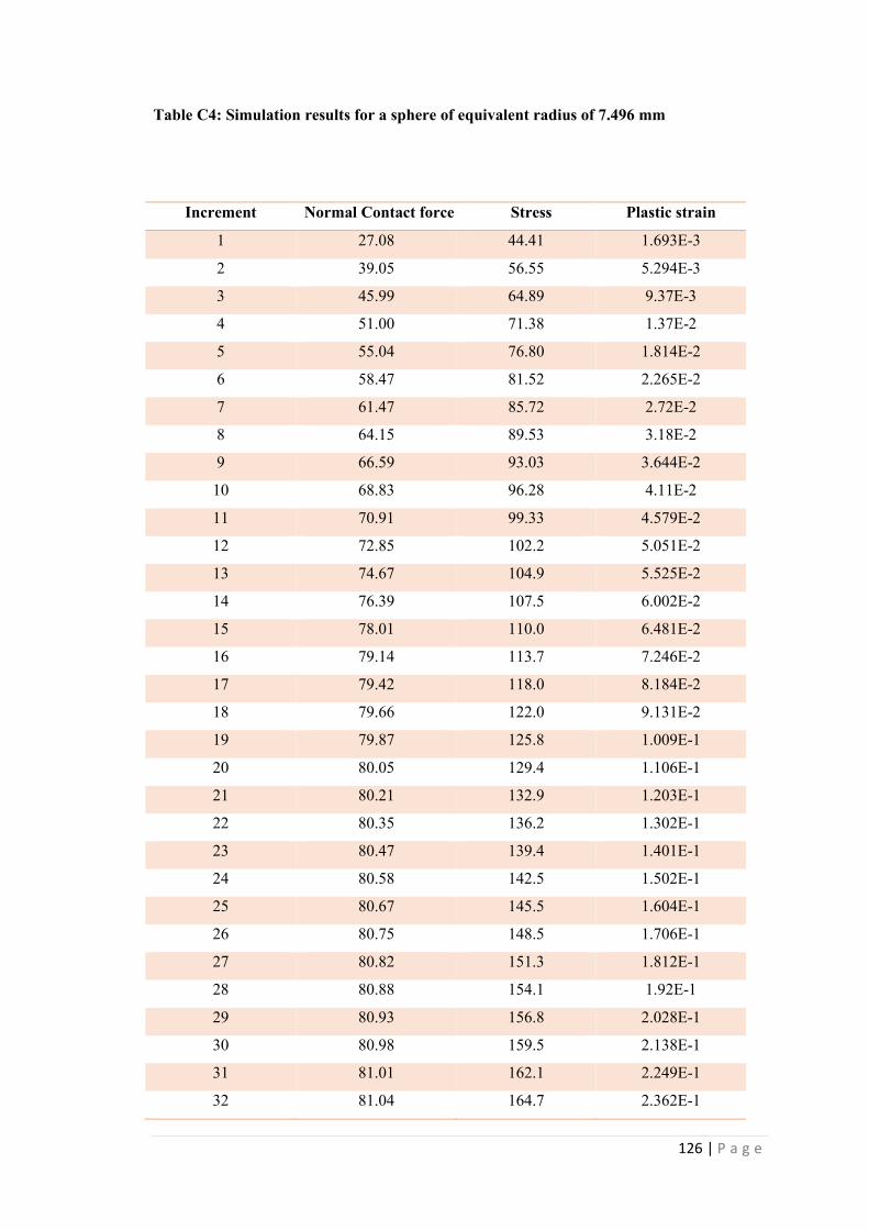
126 | P a g e

Table C4: Simulation results for a sphere of equivalent radius of 7.496 mm

Increment Normal Contact force Stress Plastic strain

1 27.08 44.41 1.693E-3

2 39.05 56.55 5.294E-3

3 45.99 64.89 9.37E-3

4 51.00 71.38 1.37E-2

5 55.04 76.80 1.814E-2

6 58.47 81.52 2.265E-2

7 61.47 85.72 2.72E-2

8 64.15 89.53 3.18E-2

9 66.59 93.03 3.644E-2

10 68.83 96.28 4.11E-2

11 70.91 99.33 4.579E-2

12 72.85 102.2 5.051E-2

13 74.67 104.9 5.525E-2

14 76.39 107.5 6.002E-2

15 78.01 110.0 6.481E-2

16 79.14 113.7 7.246E-2

17 79.42 118.0 8.184E-2

18 79.66 122.0 9.131E-2

19 79.87 125.8 1.009E-1

20 80.05 129.4 1.106E-1

21 80.21 132.9 1.203E-1

22 80.35 136.2 1.302E-1

23 80.47 139.4 1.401E-1

24 80.58 142.5 1.502E-1

25 80.67 145.5 1.604E-1

26 80.75 148.5 1.706E-1

27 80.82 151.3 1.812E-1

28 80.88 154.1 1.92E-1

29 80.93 156.8 2.028E-1

30 80.98 159.5 2.138E-1

31 81.01 162.1 2.249E-1

32 81.04 164.7 2.362E-1

127 | P a g e

Increment Normal Contact force Stress Plastic strain

33 81.06 167.3 2.476E-1

34 81.08 169.8 2.591E-1

35 81.09 172.3 2.708E-1

36 81.10 174.7 2.826E-1

37 81.11 177.1 2.945E-1

38 81.11 179.5 3.065E-1

39 81.10 181.9 3.187E-1

40 81.10 184.2 3.31E-1

41 81.09 186.5 3.435E-1

42 81.08 188.8 3.562E-1

43 81.07 191.1 3.691E-1

44 81.06 193.4 3.821E-1

45 81.05 195.7 3.954E-1

46 81.03 198.0 3.954E-1

47 81.02 200.2 4.088E-1

48 81.00 202.5 4.225E-1

49 80.98 204.8 4.364E-1

50 80.96 207.0 4.505E-1

128 | P a g e

ANNEXURE D

Table D-1:Fatigue testing recordings for sample 1

04 November 2014 00:00:00 00:05:00 00:05:00

04 November 2014 00:00:00 00:15:00 00:15:00

05 November 2014 00:03:31 00:25:25 0:21:54

05 November 2014 00:03:40 00:17:53 0:14:13

05 November 2014 00:26:38 01:08:30 0:41:52

05 November 2014 00:05:00 00:31:51 0:26:51

05 November 2014 00:00:00 01:00:00 1:00:00

05 November 2014 00:00:00 00:26:26 0:26:26

05 November 2014 00:00:00 00:12:03 0:12:03

06 November 2014 00:00:00 01:14:31 1:14:31

06 November 2014 00:00:31 00:08:35 0:08:04

06 November 2014 00:01:30 00:38:30 0:37:00

06 November 2014 00:06:00 00:16:31 0:10:31

06 November 2014 00:00:00 00:00:00 0:00:00

06 November 2014 00:00:00 00:00:00 0:00:00

06 November 2014 00:00:00 00:00:00 0:00:00

06 November 2014 00:01:54 02:21:54 2:20:00

07 November 2014 0:03:30 0:18:36 0:15:06

07 November 2014 0:19:05 03:43:09 3:24:04

07 November 2014 00:03:40 02:09:55 2:06:15

10 November 2014 00:00 01:00:00 1:00:00

10 November 2014 00:00:00 00:13:14 0:13:14

10 November 2014 00:00:00 05:30:00 5:30:00

11 November 2014 00:00:00 07:30:00 7:30:00

12 November 2014 00:00:00 07:35:06 7:35:06

13 November 2014 00:00:00 07:30:00 7:30:00

14 November 2014 08:21:00 10:54:00 2:33:00

14 November 2014 11:01:00 11:37:07 0:36:07

14 November 2014 11:37:00 13:40:00 2:03:00

14 November 2014 02:28:00 04:46:00 2:18:00

17 November 2014 00:00:00 07:00:00 7:00:00

18 November 2014 00:00:00 08:05:30 8:05:30

19 November 2014 00:00:00 09:01:09 9:01:09

20 November 2014 00:00:00 02:30:00 2:30:00

21 November 2014 00:00:00 07:10:00 7:10:00

24 November 2014 00:00:00 07:08:00 7:08:00

25 November 2014 00:00:00 07:48:55 7:48:55

27 November 2014 08:52:00 10:16:00 1:24:00

27 November 2014 00:00:00 01:51:36 1:51:36

27 November 2014 00:00:00 00:52:00 0:52:00

27 November 2014 00:00:00 00:58:40 0:58:40

27 November 2014 00:00:00 02:00:00 2:00:00

02 December 2014 00:00:00 02:35:00 2:35:00

03 December 2014 00:00:00 00:46:00 0:46:00

129 | P a g e

03 December 2014 00:00:00 05:25:00 5:25:00

04 December 2014 00:00:00 01:45:00 1:45:00

05 December 2014 00:00:00 00:56:00 0:56:00

05 December 2014 00:00:00 01:19:00 1:19:00

08 December 2014 00:00:00 03:54:00 3:54:00

08 December 2014 00:00:00 03:00:00 3:00:00

09 December 2014 00:00:00 06:37:00 6:37:00

10 December 2014 00:00:00 04:07:00 4:07:00

12 December 2014 00:00:00 02:00:00 2:00:00

12 January 2015 00:00:00 06:45:00 6:45:00

13 January 2015 00:00:00 07:00:00 7:00:00

14 January 1900 00:00:00 03:28:00 3:28:00

15 January 2015 00:00:00 03:30:00 3:30:00

16 January 2015 00:00:00 04:04:00 4:04:00

19 January 2015 00:00:00 01:20:00 4:04:00

20 January 2015 00:00:00 08:10:00 8:10:00

21 January 1900 00:00:00 3:37:00 8:53:35

22 January 2015 0:00:00 8:00:00 8:00:00

23 January 2015 0:00:00 8:30:00 8:30:00

26 January 1900 0:00:00 7:00:00 7:00:00

27 January 2015 0:00:00 6:01:00 6:01:00

28 January 2015 0:00:00 2:00:00 2:00:00

29 January 2015 0:00:00 8:00:00 8:00:00

30 January 2015 0:00:00 5:09:00 5:09:00

02 February 2015 0:00:00 3:32:00 3:32:00

03 February 2015 0:00:00 7:20:00 7:20:00

04 February 2015 0:00:00 8:00:00 8:00:00

05 February 2015 0:00:00 8:00:00 8:00:00

06 February 2015 0:00:00 4:49:00 4:49:00

09 February 2015 0:00:00 9:00:00 9:00:00

10 February 2015 0:00:00 2:40:00 2:40:00

11 February 2015 0:00:00 5:00:00 5:00:00

12 February 2015 0:00:00 7:30:00 7:30:00

13 February 2015 0:00:00 8:15:00 8:15:00

16 February 2015 0:00:00 8:18:00 8:18:00

17 February 2015 0:00:00 3:01:00 3:01:00

18 February 2015 0:00:00 7:31:00 7:31:00

19 February 2015 0:00:00 6:20:00 6:20:00

20 February 2015 0:00:00 8:00:00 8:00:00

23 February 2015 0:00:00 5:40:00 5:40:00

24 February 2015 0:00:00 8:00:00 8:00:00

25 February 2015 0:00:00 4:04:00 4:04:00

3.5 months 344:35:42

50862222

50,9

Total No. of Cycles

Cycles in Million cycles

Total Duration