1

The Effect of Disability Insurance on Beneficiaries’ Mortality1

May 2015

Alexander Gelber UC Berkeley and NBER

Timothy Moore

George Washington University and NBER

Alexander Strand Social Security Administration

Abstract

We study how U.S. Social Security Disability Insurance (DI) payments affect beneficiaries’ mortality. The formula linking DI payments to past earnings has “bend points,” or discontinuous changes in the marginal replacement rate, allowing us to use a regression kink design. Using Social Security Administration microdata on all new DI beneficiaries from 1997 to 2009, we document a substantial effect of DI payment amounts on mortality, particularly for the lowest-income beneficiaries. Our preferred estimates suggest that at the lower bend point, an increase of $1,000 in annual DI payments decreases beneficiaries’ probability of mortality over the subsequent four years by 0.47 percentage points per year, corresponding to an elasticity of -1.11. These large effects suggest that DI transfer payments have benefits that have not previously been recognized in analyses of the benefits and costs of DI.

Keywords: Social Security, Disability Insurance, Income, Health, Mortality, Regression Kink Design

1 This research was supported by the U.S. Social Security Administration through grant DRC12000002-02-00 to the National Bureau of Economic Research as part of the SSA Disability Research Consortium. The findings and conclusions expressed are solely those of the authors and do not represent the views of SSA, any agency of the Federal Government, or the NBER. We thank Thuy Ho and Paul O’Leary for helping us with the Disability Analysis File data, and we thank Zhuan Pei, Lesley Turner and David Weaver for helpful suggestions. We thank the UC Berkeley Burch Center for research support. All errors are our own.

2

I. Introduction

A key issue in health economics and public economics is how income—or income from

transfer programs specifically—affects health outcomes. The literature on the effects of income

or transfer programs on health has a long history, reaching mixed conclusions in different

contexts.2

Social Security Disability Insurance (DI) is a part of the safety net that targets people

whose health affects their ability to work. Around five percent of 25-64 year-olds receive DI.

Approximately seven percent of the federal budget is spent on DI and the medical care that is

provided through DI-related Medicare eligibility, while a further two percent is spent on cash

payments and Medicaid eligibility for low-income disabled workers through the Supplemental

Security Income (SSI) program (U.S. Treasury 2013).

A sizeable body of research has established that DI has substantial work disincentive

effects.3 This raises the possibility that DI has not only direct costs through transfers but also

substantial moral hazard costs. In light of reductions in the volatility of income or consumption

due to DI (e.g. Chandra and Samwick 2005, Ball and Low 2009, Deshpande 2014), the literature

has found mixed answers about the sign of the welfare effect of increased DI payments (Bound

et al. 2004, Meyer and Mok 2014, Low and Pistaferri 2015).4

Much less work has documented potential benefits of DI specifically in terms of

improving health outcomes. Weathers and Stegman (2012) use the Accelerated Benefits

demonstration project to examine the effects of expanding the health insurance coverage of

newly entitled DI beneficiaries, finding positive impacts on self-reported health and no impact on

mortality. Garcia-Gomez and Gielen (2014) find that stricter eligibility criteria for DI in Holland

lead to greater hospitalizations and mortality among women, but lower mortality among men.5

2 For example, see Kitagawa and Hauser 1973, Preston 1975, Preston and Taubman 1994, Ettner 1996, Deaton and Paxson 2001, Deaton 2001, Lindahl 2005, Snyder and Evans 2006, Wilkinson and Pickett 2006, Cutler, Deaton, and Lleras-Muney 2006, Sullivan and von Wachter 2009 and Akee et al. 2013. 3 See Bound 1989, Gruber and Kubik 1997, Gruber 2000, Black, Daniel, and Sanders 2002, Autor and Duggan 2003, Chen and van der Klaauw 2008, von Wachter, Manchester and Song 2011, Maestas, Mullen and Strand 2013, French and Song 2014, Autor, Maestas, Mullen and Strand 2015, Weathers and Hemmeter 2011, Campolieti and Riddell 2012, Kostøl and Mogstad 2014, Gubits et al. 2014, Coile 2015, Borghans, Gielen and Luttmer 2014, Moore 2015, Gelber, Moore, and Strand 2015. For a review of earlier work, see Bound and Burkhauser (1999). 4 See Diamond and Sheshinski (1995) for a theoretical exploration of optimal DI. 5 Singleton (2009) examines how Veterans’ Administration Disability Compensation affects diabetes detection. See Milligan and Wise (2011) for a review of historical trends across and within countries in mortality, health, employment, and disability insurance.

3

However, none of this work has examined the effects of DI payments on health outcomes. One

reason is the difficulty in identifying causal effects on health for a program that specifically

targets people whose health is poor.

We estimate the effect of DI payments on mortality using the details of the formulas that

determine benefit amounts. The DI benefit amount is defined as the Primary Insurance Amount

(PIA) subject to a family maximum. The PIA is a function of the persons earnings history,

operationalized as Average Indexed Monthly Earnings (AIME).6 The benefit formula replaces

AIME at a higher rate for beneficiaries with low average earnings. As shown in Figure 1, the

marginal replacement rate changes around several “bend points” in the schedule for converting

AIME to PIA. Below a threshold level of AIME, the marginal replacement rate is 90 percent;

between this threshold and the next, the marginal replacement rate is 32 percent; and above the

second threshold, the rate is 15 percent. The point where the marginal replacement rate changes

from 90 to 32 percent is called the “lower bend point” and the point where the marginal

replacement rate changes from 32 to 15 percent is called the “upper bend point.” In addition, the

rules for the family maximum imply that the marginal replacement rate for the family’s

combined worker and dependent benefits changes from 85 percent to 48 percent at a point

between the two bend points. We refer to this point as the "family maximum bend point." 7

Using these bend points, we implement a “Regression Kink Design (RKD)” (Nielsen,

Sorensen and Taber 2010, Card, Lee, Pei and Weber 2012). Intuitively, the technique is based on

observed changes in the slope of the relationship between mortality and lifetime earnings around

the bend points. We interpret these changes as the causal effect on health of changes in

replacement rates if the claimants in a narrow band around the bend points can be viewed as

similar to the population in a randomized experiment. More specifically, claimants that are close

to the bend points are like a treatment and a control group if they are not able to control on which

side of the bend point they fall. In this sense, each bend point creates an experiment that can be

used to estimate the causal effect relevant to the population with AIME levels near the formula

bend points (Local Average Treatment Effect (LATE)).

6 AIME is a measure of earnings in Social Security-covered employment over the individual’s highest-earning years (the number of years used in the calculation varies by age). 7 This is the different from kinks in the family maximum formulas related to benefits paid from Social Security Retirement and Survivors Insurance.

4

We investigate whether the data support this quasi-experimental interpretation. First, we

show that the population that is not affected by the bend points – that is, non-beneficiaries – does

not experience a shift in mortality around the bend points (placebo tests). Second, we show that

the population characteristics and population counts do not shift around the bend points

(covariate balance tests). This gives indirect support to the idea that claimants do not manipulate

their position relative to the bend points. Third, we show that shifts in mortality of similar

magnitude do not occur at other points in the distribution of AIME away from the bend points

(placebo kink tests).

With a large sample size of 3,648,988 beneficiaries in the full sample, we document

evidence that DI payments reduce mortality, particularly among the lowest-income beneficiaries

where the effects are large. Our baseline estimates suggest that at the lower bend point, an

increase of $1,000 in annual DI payments decreases beneficiaries’ probability of mortality over

the subsequent four years by 0.47 percentage points per year, corresponding to an elasticity of -

1.11. We find some evidence of a reduction in mortality at the family maximum bend point,

though the effect is smaller and less robust in this case. At the upper bend point, we find no

robust evidence of an effect, though our confidence intervals cannot rule out substantial effects.

The estimates are notable in light of the large value of a statistical life (VSL) (Viscusi and

Aldy 2003, in $2013). This is important in evaluating the costs of DI relative to the benefits,

particularly around the lower bend point where we estimate large effects. Our mortality gains

suggest that within any plausible VSL and estimate of the social costs of DI, the mortality

benefits of additional DI transfer income to the lowest-income beneficiaries would be of the

same order of magnitude as the costs. This suggests an important benefit that has not been

recognized in previous estimates of optimal disability insurance benefit levels.

The remainder of the paper is structured as follows. Section II describes the policy

environment. Section III explains our identification strategy. Section IV describes the data.

Section V shows our graphical analysis and RKD estimates of the effects. Section VI concludes.

5

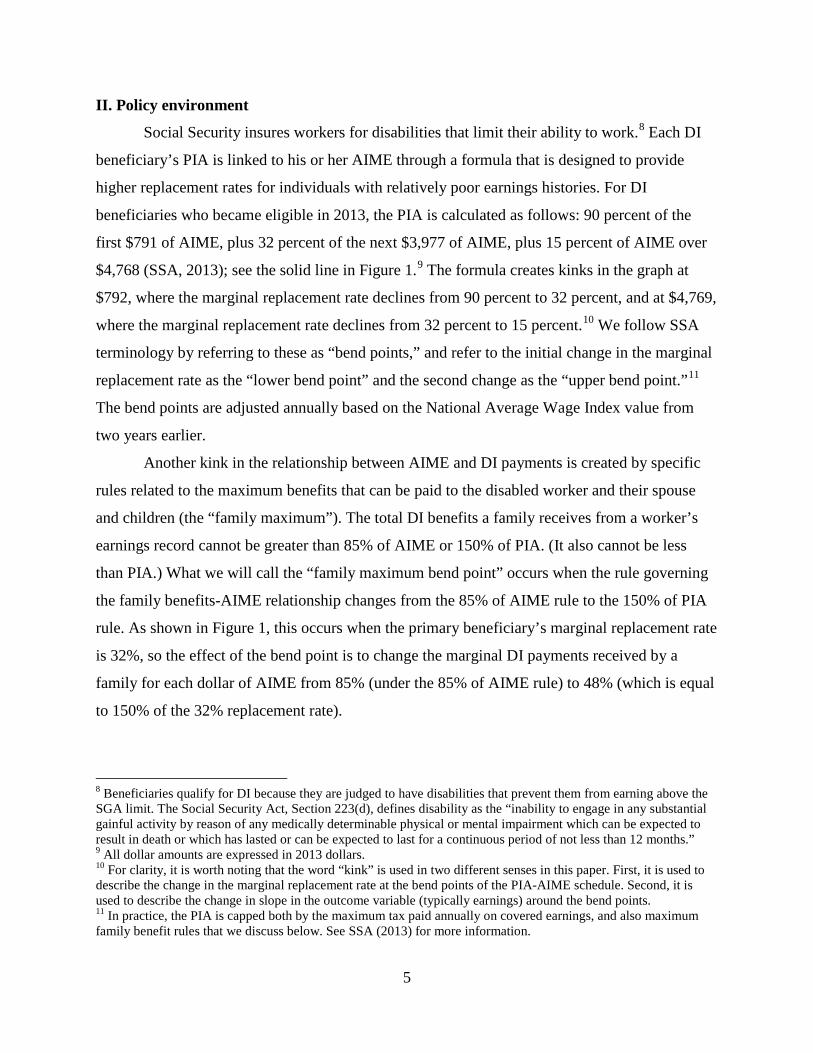
II. Policy environment

Social Security insures workers for disabilities that limit their ability to work.8 Each DI

beneficiary’s PIA is linked to his or her AIME through a formula that is designed to provide

higher replacement rates for individuals with relatively poor earnings histories. For DI

beneficiaries who became eligible in 2013, the PIA is calculated as follows: 90 percent of the

first $791 of AIME, plus 32 percent of the next $3,977 of AIME, plus 15 percent of AIME over

$4,768 (SSA, 2013); see the solid line in Figure 1.9 The formula creates kinks in the graph at

$792, where the marginal replacement rate declines from 90 percent to 32 percent, and at $4,769,

where the marginal replacement rate declines from 32 percent to 15 percent.10 We follow SSA

terminology by referring to these as “bend points,” and refer to the initial change in the marginal

replacement rate as the “lower bend point” and the second change as the “upper bend point.”11

The bend points are adjusted annually based on the National Average Wage Index value from

two years earlier.

Another kink in the relationship between AIME and DI payments is created by specific

rules related to the maximum benefits that can be paid to the disabled worker and their spouse

and children (the “family maximum”). The total DI benefits a family receives from a worker’s

earnings record cannot be greater than 85% of AIME or 150% of PIA. (It also cannot be less

than PIA.) What we will call the “family maximum bend point” occurs when the rule governing

the family benefits-AIME relationship changes from the 85% of AIME rule to the 150% of PIA

rule. As shown in Figure 1, this occurs when the primary beneficiary’s marginal replacement rate

is 32%, so the effect of the bend point is to change the marginal DI payments received by a

family for each dollar of AIME from 85% (under the 85% of AIME rule) to 48% (which is equal

to 150% of the 32% replacement rate).

8 Beneficiaries qualify for DI because they are judged to have disabilities that prevent them from earning above the SGA limit. The Social Security Act, Section 223(d), defines disability as the “inability to engage in any substantial gainful activity by reason of any medically determinable physical or mental impairment which can be expected to result in death or which has lasted or can be expected to last for a continuous period of not less than 12 months.” 9 All dollar amounts are expressed in 2013 dollars. 10 For clarity, it is worth noting that the word “kink” is used in two different senses in this paper. First, it is used to describe the change in the marginal replacement rate at the bend points of the PIA-AIME schedule. Second, it is used to describe the change in slope in the outcome variable (typically earnings) around the bend points. 11 In practice, the PIA is capped both by the maximum tax paid annually on covered earnings, and also maximum family benefit rules that we discuss below. See SSA (2013) for more information.

6

We therefore have three kinks that change the marginal relationship between DI benefits

and AIME: the lower and upper bend points that affect the DI payments to the primary

beneficiary, and the family maximum bend point that affects the total DI payments whenever the

primary beneficiary has a dependent.12 However, there are two characteristics of the program

rules that weaken these relationships for some beneficiaries. One is the family maximum rules as

they apply at locations away from the family maximum kink. The other is how SSI payments

interact with DI payments for some beneficiaries eligible for both programs.

The family maximum rules complicate the analysis at the lower bend point by changing

the relationship between DI payments and AIME. This is apparent in Figure 1. At low values of

AIME, the relevant rule is that the family benefits must be at least as large as PIA (because the

initial 90% marginal replacement rate is less than the “85% of AIME” rule), The family

maximum is equal to the PIA until the PIA is equal to 85% of AIME. In 2013, this occurred at an

AIME that is $75 above the lower bend point. Between this level and family maximum bend

point described above, the “85% of AIME” rule applies. This means that, when considering total

family DI payments, the marginal replacement rate is 90 percent of AIME up to the lower bend

point, then 32 percent for the next $75 of AIME, then 85 percent for the next $1,000 of AIME.

This creates measurement issues in the region of the lower bend point, although not in the region

of the family maximum bend point and upper bend point.13,14

SSI payments also affect the relationship between AIME and payment amounts,

especially in the region of the lower bend point. SSI is available to disabled individuals who,

apart from a home and a car, have no more than a few thousand dollars in assets. SSI recipients

are also subject to different and more restrictive earnings rules. SSI provides an income floor that

does not depend on AIME or any other measure of past earnings. In 2013, the federal benefit rate

for SSI-eligible individuals was $710 per month. Dually-eligible DI beneficiaries whose PIA is

greater than their SSI payment only receive SSI payments during their DI waiting period, which

12 A dependent receives 50% of the worker’s PIA. Given that the family maximum is always limited to 150% of PIA, this means that a family with one dependent will receive the same as a family with more than one dependent. Note that this is not the case for Social Security Retirement and Survivors Insurance. 13 While this suggests we should remove beneficiaries with dependents in the region of the lower bend point, differential reporting of dependents can occur because the family maximum being initially equal to PIA means no extra payments come from reporting a dependent. This measurement issue is discussed later in the paper. 14 The 150% of PIA applies in the region of the upper bend point, which means that the marginal rate for the family maximum changes from 48% (150% of 32%) to 22.5% (150% of 15%). Later in the paper, we examine the results at the upper bend point for beneficiaries without dependents.

7

is five months after the date of disability onset, while dually-eligible DI beneficiaries whose PIA

is below the federal SSI payment are “topped up” to the SSI income floor, breaking the link

between AIME and total disability payments. In other words, for the dual-eligible group, we

would not necessarily expect to observe a kink in the slope of their net disability benefits as a

function of AIME near that bend point because an additional dollar in DI payments reduces their

SSI payments by one dollar.15 The SSI monthly payment amount of $710 is nearly identical to

$712, the PIA they would receive if they had an AIME that put them at the lower bend point.

The substantial majority of DI recipients are dual-eligible for SSI in the region of the lower bend

point (approximately two-thirds of our potential sample in the region of the lower bend point, as

shown in Appendix Figure A6). For this large group of dual-eligibles, there is no change in the

marginal replacement rate (net of both SSI and DI payments) at the lower bend point.

In order to use the regression kink design to generate causal estimates, beneficiaries

should not be able to locate at specific AIME values. The policy environment helps in this

regard, as steps involved in calculating the AIME are as follows: (i) determine the number of

years between the year after an individual turns 21 and the year of eligibility for DI; (ii) convert

earnings in each of these years to the year of eligibility using the National Average Wage Index,

which is based on the growth in earnings two years earlier (e.g., 2007 earnings are scaled by

Index values for 2005); (iii) remove one-fifth of the lowest earnings years (rounded to the next

lower integer), up to a maximum of five years;16 (iv) average the earnings across the remaining

years; and (v) divide by 12 to convert to monthly amounts. For most DI beneficiaries, many

years go into the AIME calculation: in 2012, 65.5 percent of DI entrants were aged 50 years or

older, and so have a relevant earnings history that lasts 28 or more years (SSA, 2013).

III. Identification strategy and interpretation of estimates

Recent work has shown that under certain conditions, a change in the slope of treatment

intensity can be used to identify local treatment effects by comparing the relative magnitudes of

15 The amount of the SSI payment also depends on other unearned income besides the DI benefit and the earned income of family members, as well as in-kind support. 16 At least two years must be used in the AIME computation. Disabled workers who receive fewer than three “dropout years” (i.e. low-earning years that are discarded from the AIME calculation) under the rule guaranteeing that one-fifth of earnings years are dropped may be credited with additional dropout years based on child care if they had no earnings and a child aged under three years (up to a total of three additional years).

8

the kink in the assignment variable and the induced kink in the outcome variable. This is known

as a “Regression Kink Design” (RKD). Estimates can be interpreted as a treatment-on-the-

treated parameter (Card et al. 2012).

In our context, the treatment intensity is the size of DI benefits (i.e. PIA), the assignment

variable is the average value of past earnings (i.e. AIME) observed when the individual first

applies for DI, and our primary outcome variable is beneficiaries’ probability of death after

entering DI. An extra dollar in AIME leads to a smaller change in PIA just above a bend point

than just below it. This discontinuously changes the slope of DI payments as a function of AIME

at a bend point, while the slope of the relationship between other determinants of earnings (such

as human capital, work experience, etc.) and AIME should not change discontinuously around

the bend points. In this case, we can estimate the causal effect of DI benefits on the probability of

mortality by comparing the change in the slope of the mortality-AIME relationship to the change

in the slope of the PIA-AIME relationship at the bend point. If DI payments decrease mortality,

then the slope in the mortality-AIME relationship will be steeper above a bend point than below

it. Of course, we would expect the opposite change in slope if higher benefits increase mortality.

Mathematically, we want to estimate the marginal effect of DI benefits (B) on the

probability of mortality (Y). Benefits depend on AIME (A). Using the RKD, we can estimate the

marginal effect of benefits on the probability of mortality around a given bend point A0 using the

following equation:

(1)

That is, the marginal effect we estimate is the change at the bend point in the slope of mortality

probability as a function of AIME, divided by the change at the bend point in the slope of DI

benefits as a function of AIME.

Identification of the effect of DI benefits on mortality relies on two assumptions (Card et

al., 2012). First, the direct marginal effect of AIME on the outcome must be smooth. Second, the

density of the unobserved error component evolves smoothly with AIME, so that the derivative

of its conditional probability density function is continuous at the bend point. These assumptions

may not hold if we observe sorting in relation to the bend points, either because we observe a

change in slope or level of the density of the assignment variable at the bend point or because we

E �𝜕𝜕𝜕𝜕𝜕𝜕𝜕𝜕

|𝐴𝐴 = 𝐴𝐴0� = limA→A0

+∂E[Y|A = A0]

∂A − limA→A0−∂E[Y|A = A0]

∂AlimA→A0

+∂B(A)∂A − limA→A0

−∂B(A)∂A

9

observe a change in the distribution of predetermined covariates at the bend point. In our context,

there are several reasons why it would be surprising to see individuals sorting around the bend

points. First, the value of AIME that we use is from before individuals go on DI, implying that it

cannot be affected by earnings after people are on DI. Second, individuals would typically have

to change their earnings over long periods of time to change their AIME substantially.17 As

discussed in the previous section, close to two-thirds of individuals entering DI in 2012 were

aged 50 years or older and so have a relevant earnings history that lasts 28 or more years. If

disability onset occurs relatively unexpectedly, it may be infeasible to choose earnings long in

advance to change the earnings history substantially. Third, as we described above, the

calculation of the AIME on the basis of an individual’s earnings history is complex, involving

inflation of earnings from long-past years using the National Average Wage Index, which

implies that it is likely to be difficult for individuals to accurately estimate their AIME and,

therefore, where their earnings history will put them in relation to the bend points. Finally,

disabled workers typically experience decreasing earnings trajectories in the years before

applying for DI (von Wachter, Song and Manchester, 2011). A year just prior to applying for DI

would in many cases be among the lowest-earning years and would therefore be excluded from

the AIME calculation. All of these factors suggest that it is extremely difficult for an individual

to choose an AIME in relation to the bend points.

In measuring the denominator of (1), note that the determination of PIA on the basis of

AIME is deterministic; by law the marginal replacement rate changes around the bend points in

the ways described above. Moreover, observed PIA closely matches the values estimated when

using the Social Security formula.18 Accordingly, our main specification uses a “sharp” RKD

where we only need to estimate the numerator, which is the change in the slope of the

conditional expectation function of earnings at the bend point. If the relationship between an

outcome Y and AIME is linear, then the numerator can be estimated by running regression

models of the form:

(2)

17 AIME calculations are based on earnings in, at most, the 35 highest-earning years, beginning the year after an individual turns 21. Shorter periods apply for younger claimants. 18 We show that the average difference between actual and estimated PIA is $1.80 around the lower bend point, $2.18 around the family maximum bend point, and $2.62 around the upper bend point.

10

where in our context Y is typically the average annual mortality rate over the first four years on

DI, A is AIME, A0 is the level of AIME at the bend point, D = 1[A≥A0] is an indicator for being

above the bend point threshold, and the change in the slope of the graph of average earnings

against AIME at the bend point is given by β2. We limit the analysis to observations for which

|A-A0|≤h, where h is the bandwidth size.

Our assignment variable in the sharp RKD is an individual’s initial AIME, i.e., the value

of AIME when they apply for DI. Gelber, Moore, and Strand (2015) show that accounting for

changes in AIME over time using a “fuzzy RKD” changes the results negligibly.

Interest in RKD is relatively recent, and many of the details surrounding the econometric

theory and empirical implementation of the approach are unsettled. One is the choice of

bandwidth.19 At the lower bend point, the bandwidth is constrained to $500 by low AIME value

at which it occurs.20 At the family maximum bend point, the bandwidth is constrained to $900 by

the distance to the lower bend point. At the upper bend point, we selected $1,500 as our primary

bandwidth.21 We examine the robustness of our analysis by estimating regressions using

different bandwidths and find similar results across a wide range of bandwidths.

Another issue is the order of the polynomial chosen to estimate the relationship between

the assignment and outcome variable. We call model (2) the “linear” specification because the

control for (A-A0) is linear. Local linear regression is appealing in our context, where there is a

constant marginal relationship between AIME and the PIA away from the bend points. Card et

al. (2012) and Dong (2012) argue that the derivative is likely to suffer from boundary bias. Card

et al. (2012) show that local quadratic regression should have smaller bias than local linear

regression using the same bandwidth, although with much higher variance. They use both linear

and quadratic specifications in their analysis. Calonico, Cattaneo and Titiunik (2014) propose an

RKD estimator where the quadratic specification can be used to correct for the bias in the linear

estimator. In a recent working paper, Ganong and Jaeger (2014) argue that using cubic splines

perform better than other estimators and recommend the quadratic specification of Calonico,

19 Following standard practice in RD and common practice in RKD studies, we always use symmetric bandwidths. 20 At the lower bend point, the AIME of $791 constrains the bandwidth to a value less than that. In practice, there are almost no observations below an AIME of $200, as beneficiaries with such low earnings are unlikely to have sufficient quarters of coverage to qualify for DI. 21 The bandwidths for the lower and upper bend points are the same as those in Gelber, Moore and Strand (2015).

11

Cattaneo and Titiunik’s estimator with robust bias correction (where the default form of bias

correction means this is equivalent to a local cubic estimator).

Our approach is to implement linear, quadratic and cubic versions of equation (2) (i.e.

controlling for only (A-A0), adding a term in (A-A0)2, or adding an additional control for (A-A0)3,

respectively) to investigate the robustness of our results across all of these different choices.

Similarly to Card et al. (2012), we use a parsimonious test for a change in slope by examining

whether there is a change in the linear term of the polynomial above the bend point (i.e.

examining whether β2 in (2) is significantly different from zero).

Another issue is whether or not to allow for a discontinuity at the bend point in the level

of the outcome variable. When treatment effects are heterogeneous, the imposition of continuity

is necessary for change in slope at the bend point to be considered a causal parameter (Card et

al., 2012). However, there are concerns that imposing continuity increases the likelihood of

spurious results (Ando, 2013). Again, we will implement specifications that impose continuity

and others that allow for a discontinuity at the bend point.

A third area of some discussion is the role of covariates. An attractive feature of the RKD

is that the lack of sorting around the kink should result in smoothness in predetermined

covariates, and the ability to identify causal effects without relying on extensive covariates.

However, Ando (2013) argues the addition of covariates minimizes the likelihood of spurious

results. To demonstrate the robustness of our results, we try both specifications where we control

for predetermined covariates and other specifications where we omit these controls.

Thus, for each sample and outcome we will generally produce estimates using nine

regressions: base versions of the linear, quadratic and cubic regressions; a version of each of

these that allows for a discontinuity in the level of the outcome variable at the bend point; and a

version of each of these that includes predetermined covariates.

Our main bin size is $50, which is the largest bin size at which all dependent variables

pass the two tests of excess smoothing for regression discontinuity designs recommended by Lee

and Lemeieux (2010).22 We take the mean of variables within each bin and run the regression

22 We follow Landais (2014) in applying this to an RKD context. The first test assesses whether using narrower bins provides a better fit to the data. It is implemented by comparing the R-squared from a regression with dummy variables for each bin of width w to the R-squared from a regression with dummy variables for each bin of width w/2. The bin size w is decreased until the resulting F statistic is not statistically significant. The second test is based on the idea that a bin width is too wide if, within each bin, there is a systematic relationship between the outcome

12

using the aggregated data, weighting bins by the number of observations in each bin. By

averaging data within each bin, we estimate standard errors that we view as conservative,

following one of Lee and Lemieux’s (2010) suggestions in the Regression Discontinuity context.

We follow Card et al. (2012) in using White robust standard errors. We also show robustness to

estimating all nine regressions at the individual level, and to estimating the regressions with a

variety of other bin sizes, in both cases also using robust standard errors.23

We interpret our results as reflecting the effects of greater DI transfer payments on

mortality. Gelber, Moore, and Strand (2015) estimate that around one-fifth of an increase in DI

payments is offset through lower earnings. Thus, the estimates of the effects of increased DI

payments on mortality could be mediated both through the increase in net income and the

decrease in earnings. Note that a priori, greater DI transfer payments could lead to either

decreases or increases in mortality. For example, increased DI transfer payments could lead

individuals to purchase more of goods that allow them to avoid mortality (e.g. a better diet or

treatment for disability-related conditions). On the other hand, increased DI transfer payments

could lead individuals to work less (as the evidence suggests), and working less could lead to

increased mortality (see e.g. Snyder and Evans 2006), for example if working improves cognitive

functioning and therefore reduces mortality.

Individuals often are not aware of the Social Security rules (Liebman and Luttmer

forthcoming). Our RKD strategy does not necessarily assume that individuals are aware of the

kink in benefits at the bend points; they could be responding, for example, to the amount of DI

payments they themselves are receiving, or their total income, which seem much more salient.

variable and the assignment variable. It is implemented by interacting each bin dummy variable with the assignment variable, regressing the outcome variable on the set of bin indicators as well as these interaction terms, and testing the joint significance of the interaction terms. The bin size w is decreased until the F-statistic on the joint test is not statistically significant. 23 Because our outcome is the mortality of a given individual over a given period, there is one observation per individual. Thus we do not have to address within-individual correlation of errors over time, and we do not have to control for time dummies. Results are similar when we include dummy variables for the year the outcome is observed and/or the year the individual goes on DI.

13

IV. Data

IV.a. Sample selection

We use administrative data from the 2010 version of the Disability Analysis File (DAF)

(previously called the Ticket Research File). The DAF is a compilation of multiple

administrative data sources from the Social Security Administration, including the Master

Beneficiary Record, Supplemental Security Record, 831 File, Numident File, and Disability

Control File. The DAF contains information on all disability beneficiaries with at least one

month of current-pay status between 1997 and 2010, including information on AIME and PIA.

The data sources that are used to construct the DAF also provide information on each

beneficiary’s demographic characteristics, including age, race, and gender; DI program activity,

including path to allowance (e.g. whether a claimant was determined to be eligible by the initial

disability examiner or through a hearings-level appeal) and the magnitude of disability payments;

and exact date of death (day, month, and year) (Hildebrand et al., 2012). We obtained updated

information on date of death through 2013 in order to extend the period over which we could

track beneficiaries’ mortality.

We choose a sample of individuals who entered DI between 1997 and 2009 and who

were aged 21 to 61 years at the time of filing. The program rules were largely consistent

throughout this time period, and we are able to observe whether these individuals died within

four years of beginning to receive DI payments. The upper age restriction to those under 61

avoids interactions with rules associated with the Social Security Old Age and Survivors

Insurance program. We also limit the sample to DI claimants who did not receive SSI at any

point in the sample period.

We clean the data by removing records with missing or imputed observations of basic

demographic information (e.g., date of birth, sex). We also remove records in which there is no

initial AIME or PIA value, or in which the stated date of disability onset used for the PIA

calculation is more than 12 months before the date of filing or 17 months after the date of filing

(the range over which documented date of disability onset should lie). In addition, we remove

individuals who have a PIA based on eligibility for DI under both their record and that of another

worker or who had not received DI payments within four years of filing. We clean the data to

remove cases in which the data contain unreliable measures of AIME by removing those with

more than four AIME changes. The SSA data systems typically have a small number of cases

14

with unusual or implausible records; these sample restrictions are similar to those generally made

when using these data (e.g., von Wachter, Song and Manchester 2011, Maestas, Mullen and

Strand 2013, Gelber, Moore and Strand 2015, Moore 2015).

We choose samples around each bend point in order to focus on the effects of that bend point on

mortality. Thus, for the family maximum bend point, we restrict to beneficiaries where the

earnings record also supports a dependent benefit. The samples for lower and upper bend points

do not have this restriction.24

IV.b. Summary statistics

Table 1 shows summary statistics. In the full sample, we use data on 3,648,988

observations. Average PIA is $1,360. PIA is a monthly measure of DI payments, so that $1,360

in monthly payments translates into an annualized value of $16,315.

In examining post-award mortality, we use a four year follow-up period. This allows us

to examine the mortality effects close to when individuals first receive DI, and after they have

had time to adjust to DI payments and rules. Four years also is the same length of time used in

Maestas, Mullen and Strand (2013) and Gelber, Moore and Strand (2015). Annual mortality rates

in the four years after first receiving DI range between 2.6 percent (fourth year after program

entry) and 7.0 percent (first year after program entry). Average age when applying is 48.6, and

53.1 percent of the sample is male. For approximately half of the sample, their primary disability

is either a musculoskeletal condition (29.7 percent) or mental disorder (20.1 percent), with

neoplasms (cancer) (11.6 percent) and circulatory conditions (largely heart disease) (10.3

percent) also common.

Since our identification strategy is based on examining earnings patterns around the bend

points, the estimates will be local to individuals in the region of these bend points. For

comparison, the table also shows the summary statistics for samples around each of the bend

points (the lower bend point, the family maximum bend point, and the upper bend point). Those

around higher bend points have higher mean PIA. The lowest mortality rates are observed for the

family maximum bend point sample, with the requirement that beneficiaries have a dependent in

24 While we would like to restrict the lower bend point sample to beneficiaries without dependents in order to deal with the measurement issues related to the family maximum rules, the lack of additional payments to dependents at low AIME values means we cannot reliably make this restriction.

15

order to be included resulting in the relatively young sample. Modestly higher mortality rates at

the lower bend point and upper bend points.

V. Graphical and regression analysis

V.a. Preliminary analysis

We begin our empirical analysis with validity checks on our empirical method. Figure 2

shows that the number of observations and its slope appears continuous around the bend points.

This finding is consistent with the possibility that DI onset occurs relatively unexpectedly,

supporting the notion that the effects we document are associated with changes in transfer

income that were not anticipated prior to going on DI. Appendix Figure 1 shows the distribution

of the means of six predetermined covariates available in the administrative data (fraction male,

fraction black, fraction allowed via hearing, fraction whose disability is a mental disorder,

fraction whose disability is a musculoskeletal condition and average age when applying for DI).

All of these appear smooth through all three of the bend points. Appendix Figure 2 shows that, as

expected, measured PIA in the dataset shows changes in slope at the bend points in AIME in

precisely the ways the policy dictates.

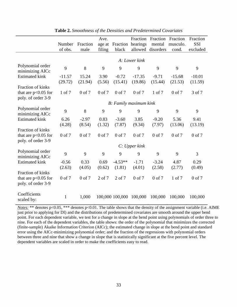
Our regressions in Table 2 confirm that the number of observations, these predetermined

covariates, and the fraction of the potential sample on SSI, are all smooth in the region of the

bend points. We adopt an approach similar to Card et al. (2012) and Turner (2014) by examining

whether the first derivative changes at the bend point, as measured by coefficient β2, when we

run separate regressions with polynomials in AIME of order between three and nine. For each

dependent variable, we select the polynomial order that minimizes the finite-sample (corrected)

Akaike Information Criterion (AICc) and report the change in slope at the bend point for that

specification. We use our baseline specification with binned covariates and outcomes, without

additional controls, and with no discontinuity in the dependent variable at the bend point. Out of

24 regressions (8 outcomes for each of three bend points), only one estimate for a change in the

slope at the bend point is significantly different from zero at the five percent level. This is likely

to be due to chance, as even randomly-generated data should produce a statistically significant

coefficient at the five percent significance level once in every 20 regressions.

Moreover, Table 2 also shows that these regressions are rarely statistically significant for

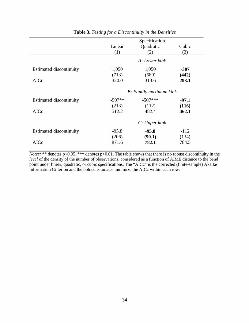
any particular polynomial order. Table 3 verifies that there is no robust evidence of a change in

16

the level of the density of the running variable around each of the three kinks under linear,

quadratic, or cubic specifications. (While there is a statistically significant discontinuity at the

family maximum bend point in the linear and quadratic specifications, the AIC-minimizing

specification at this bend point is the cubic specification, where there is an statistically

insignificant change in the level.)

All of these results suggest that individuals do not appear to locate their AIME

strategically and RKD methods are appropriate for estimating causal treatment effects. As we

discussed above, it is not surprising to find that there is no sorting around the bend points given

that it is difficult to understand, calculate and manipulate AIME.

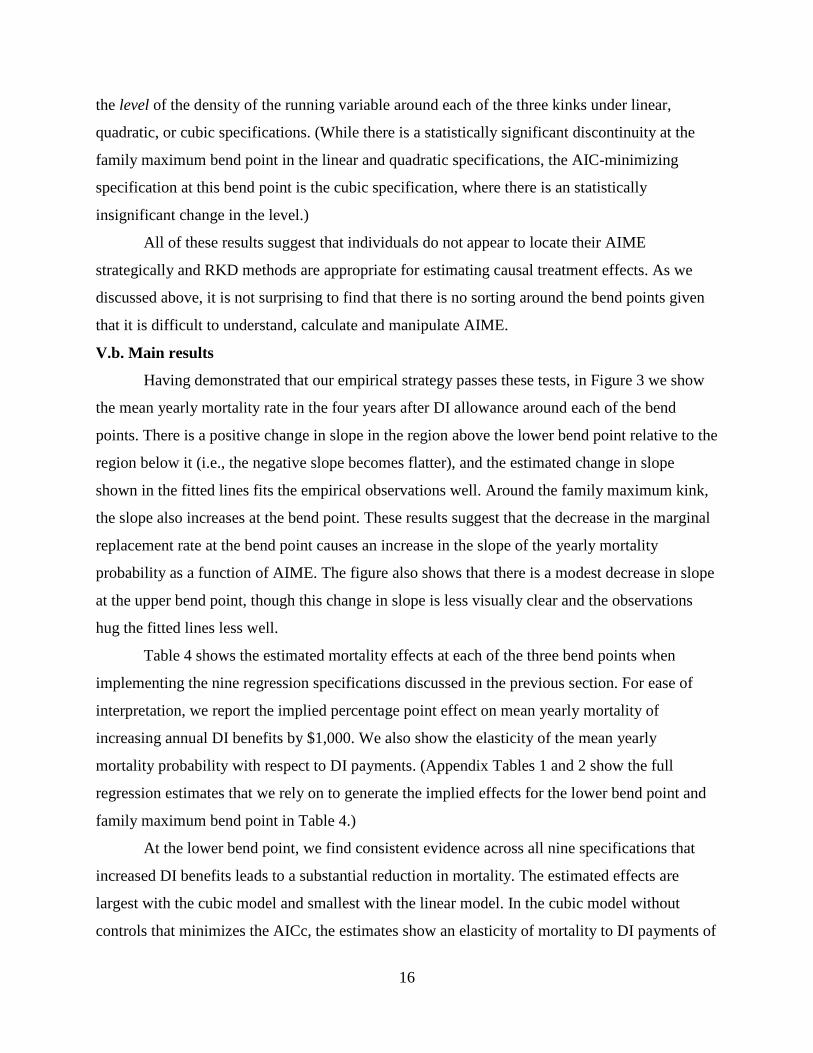
V.b. Main results

Having demonstrated that our empirical strategy passes these tests, in Figure 3 we show

the mean yearly mortality rate in the four years after DI allowance around each of the bend

points. There is a positive change in slope in the region above the lower bend point relative to the

region below it (i.e., the negative slope becomes flatter), and the estimated change in slope

shown in the fitted lines fits the empirical observations well. Around the family maximum kink,

the slope also increases at the bend point. These results suggest that the decrease in the marginal

replacement rate at the bend point causes an increase in the slope of the yearly mortality

probability as a function of AIME. The figure also shows that there is a modest decrease in slope

at the upper bend point, though this change in slope is less visually clear and the observations

hug the fitted lines less well.

Table 4 shows the estimated mortality effects at each of the three bend points when

implementing the nine regression specifications discussed in the previous section. For ease of

interpretation, we report the implied percentage point effect on mean yearly mortality of

increasing annual DI benefits by $1,000. We also show the elasticity of the mean yearly

mortality probability with respect to DI payments. (Appendix Tables 1 and 2 show the full

regression estimates that we rely on to generate the implied effects for the lower bend point and

family maximum bend point in Table 4.)

At the lower bend point, we find consistent evidence across all nine specifications that

increased DI benefits leads to a substantial reduction in mortality. The estimated effects are

largest with the cubic model and smallest with the linear model. In the cubic model without

controls that minimizes the AICc, the estimates show an elasticity of mortality to DI payments of

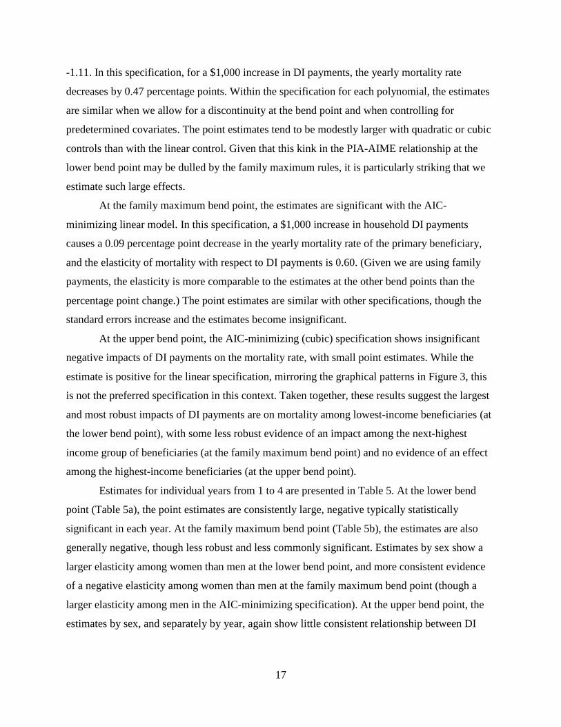
17

-1.11. In this specification, for a $1,000 increase in DI payments, the yearly mortality rate

decreases by 0.47 percentage points. Within the specification for each polynomial, the estimates

are similar when we allow for a discontinuity at the bend point and when controlling for

predetermined covariates. The point estimates tend to be modestly larger with quadratic or cubic

controls than with the linear control. Given that this kink in the PIA-AIME relationship at the

lower bend point may be dulled by the family maximum rules, it is particularly striking that we

estimate such large effects.

At the family maximum bend point, the estimates are significant with the AIC-

minimizing linear model. In this specification, a $1,000 increase in household DI payments

causes a 0.09 percentage point decrease in the yearly mortality rate of the primary beneficiary,

and the elasticity of mortality with respect to DI payments is 0.60. (Given we are using family

payments, the elasticity is more comparable to the estimates at the other bend points than the

percentage point change.) The point estimates are similar with other specifications, though the

standard errors increase and the estimates become insignificant.

At the upper bend point, the AIC-minimizing (cubic) specification shows insignificant

negative impacts of DI payments on the mortality rate, with small point estimates. While the

estimate is positive for the linear specification, mirroring the graphical patterns in Figure 3, this

is not the preferred specification in this context. Taken together, these results suggest the largest

and most robust impacts of DI payments are on mortality among lowest-income beneficiaries (at

the lower bend point), with some less robust evidence of an impact among the next-highest

income group of beneficiaries (at the family maximum bend point) and no evidence of an effect

among the highest-income beneficiaries (at the upper bend point).

Estimates for individual years from 1 to 4 are presented in Table 5. At the lower bend

point (Table 5a), the point estimates are consistently large, negative typically statistically

significant in each year. At the family maximum bend point (Table 5b), the estimates are also

generally negative, though less robust and less commonly significant. Estimates by sex show a

larger elasticity among women than men at the lower bend point, and more consistent evidence

of a negative elasticity among women than men at the family maximum bend point (though a

larger elasticity among men in the AIC-minimizing specification). At the upper bend point, the

estimates by sex, and separately by year, again show little consistent relationship between DI

18

payments and mortality. Appendix Figure 3 shows that the corresponding graphical patterns by

sex at each of the bend points mirror the regression results.

V.c. Robustness and further validity checks

We perform several exercises to further establish the robustness of the mortality

estimates. In Figure 4 and Table 6, we show results for four placebo samples. Panel A of Figure

4 shows the mortality of beneficiaries without dependents who are in the region of the family

maximum bend point. These beneficiaries are unaffected by the family maximum rules and

therefore we should not see a change in the mortality-AIME relationship at the family maximum

bend point. This is the case; moreover, the regression estimates for this sample that are presented

in Panel A of Table 6 verify that there is no robust significant change in mortality at the family

maximum bend point. A significant elasticity appears in the linear specification, though it is

much smaller than the elasticity that appears at this bend point in the main sample (-0.14

compared to -0.60) and is not the AIC-minimizing specification.

Figure 4 Panels B through D show the mortality rates for non-DI beneficiaries as a

function of AIME at each of the three bend points. We create a sample of non-beneficiaries from

the 2011 Continuous Work History Sample, a one percent sample of active Social Security

Numbers. The analysis sample is living DI-insured workers age 18-57 in 2005 who have never

applied for DI. AIME is calculated as if they had become eligible for DI during 2005. We also

use a four-year follow up period for this group and so measure mortality from 2006 to 2009.

Unsurprisingly, this non-beneficiary group has much lower mortality rates than the samples of

DI beneficiaries.

There is no increase in slope at the lower and family maximum bend points—in fact, if

anything, the slope modestly decreases at the bend points, though not sharply. At the upper bend

point, the slope decreases at the bend point more sharply, suggesting that the modest decrease in

slope at the upper bend point among beneficiaries may simply reflect a pattern that occurs in the

placebo sample. The regression estimates in Table 6 correspondingly shows that there is no

significant change in slope at the any of the bend points in the placebo sample, including at the

lower bend point. This reinforces our conclusion that there is a substantial and robust effect at

the lower bend point that does not represent a pre-existing relationship between mortality and the

distribution of AIME values.

19

Another robustness exercise is presented in Figure 5, where we show how the mortality

estimates at the lower and family maximum bend points vary as a function of the chosen

bandwidth. At the lower bend point, using the AIC-minimizing cubic specification, the estimated

mortality effects are similar to the main estimate and statistically significant at the five percent

level using bandwidths from $750 to $300 (below which the small number of observations lead

to insignificant estimates). At the family maximum bend point, using the AIC-minimizing linear

specification, the estimates are also similar and statistically significant for bandwidths from

$1,100 to $650. In both cases, the ranges over which the estimates are stable include the

bandwidth computed using the RKD bandwidth selection procedures of Calonico, Cattaneo and

Titiunik (2014).

Another approach to establishing the robustness of the estimates is to examine where the

structure of data indicates there is a kink by comparing our estimates with estimates based on

“placebo” kinks at other locations (Ganong and Jaeger, 2014). Figure 6 shows the elasticity

estimate and 95 percent confidence interval when we run the RKD regression (2) for “placebo”

kinks that are located throughout the range of AIME values covered by the bandwidths. The

figure shows that, in both the lower bend point and the family maximum samples, the largest and

most statistically significant coefficients (in absolute value) occur at the actual location of the

bend points. The contrast in real and placebo coefficients is sharper for the lower bend point

sample for than the family maximum sample, but in both cases these results suggest that a data-

driven approach would find kinks where the Social Security policy rules says they should be.

Ganong and Jager (2014) argue that RKD estimates may simply reflect a nonlinear relationship

in the data that happens to have an inflection point close to the kink. The lack of such points at

other locations in the data window minimizes the concerns that our estimates are spurious.

Table 7 shows a variety of additional robustness checks. First, to explicitly deal with the

binary nature of mortality as an outcome, we run a grouped logit model where the dependent

variable is ln[mortality rate/(1 – mortality rate)] and the coefficients are transformed into

marginal effects by multiplying them by E[(mortality rate)/(1 – mortality rate)]. This

specification generates comparable results to our main specification.

Second, individuals who received SSI were removed from the sample considered thus far.

To assess whether our estimates are robust to including SSI recipients in the sample, in Table 7

we report the earnings estimates when we include SSI recipients in our sample. As described in

20

the section on policy environment, SSI can break the link between AIME and total disability

payments. Thus, it is not surprising that we see smaller and less robust estimates of the mortality

effects at the lower and family maximum bend points (where SSI receipt is prevalent).

Third, as noted, in our main sample we drop individuals whose AIME changes more than

four times. In Table 7 we show results for the full sample when we do not restrict the number of

times that AIME may change. The coefficient estimates are slightly different but in the same

range as those in our baseline sample, which is unsurprising given the additional measurement

error in this sample.

Fourth, Table 7 shows regressions using the individual-level data (rather than collapsing

to the bin level), and alternatively with $25-wide bins or $100-wide bins. These all show

extremely similar results to our baseline estimates.

V.d. Effect heterogeneity

Table 8 shows the mortality effects at the lower and family maximum bend points in

different subgroups of the population. We report estimates using the respective AIC-minimizing

specifications, which is the cubic specification with no controls at the lower bend point and the

linear specification with no controls at the family maximum bend point. We present both the

percentage-point change in the annual mortality rate resulting from an additional $1,000 in

annual DI payments and the elasticity in mortality in relation to DI payments, as the former

provides information about absolute changes in mortality and the latter depends on the

underlying mortality rates in the subgroup.

At the lower bend point, the absolute changes in mortality are similar for younger (aged

below 45 at filing) and older (aged 45 and older at filing) beneficiaries, although the elasticity is

twice as large for the younger group than the older group because of their relatively low

mortality. There are larger absolute changes in mortality and mortality elasticities for those

initially allowed DI through an initial Disability Determination Services (DDSs) assessment than

those allowed via a hearing (after an initial denial). When breaking down the results by type of

primary disability, the largest and most significant changes in mortality are for cancers and

circulatory conditions. There are not large, clear differences by race or when individuals entered

the DI program. The differences in mortality outcomes across these groups are qualitatively

similar at the family maximum bend point.

21

VI. Conclusion

A key policy question regarding DI is the extent to which disability insurance payments

affect mortality. The graphical and regression evidence suggests that DI payments can reduce

mortality, particularly in the lowest-income groups. In particular, at the lower bend point, we

robustly find that DI payments decrease mortality quite substantially. In this group, our baseline

shows that the elasticity of mortality with respect to DI income is -1.11, and that a $1,000

increase in yearly DI payments leads to a decrease in the yearly mortality rate of 0.47 on a basis

of 3.61 percentage points (see Table 5). It is perhaps not surprising to find the largest effect of DI

payments in the lowest-income group, as DI payments are largest relative to lifetime income in

this group.

The estimates are notable in light of the large value of a statistical life (VSL), estimated

to be in the range of $9 million for prime-age workers (Viscusi and Aldy 2003, in $2013). Even

at the lower end of the plausible range of the VSL suggested by Viscusi and Aldy (2003) (around

$5.25 million), it is clear that the mortality benefits should be large within any plausible range of

the value of life. This is important in evaluating the costs of DI relative to the benefits,

particularly around the lower bend point where we estimate large effects. Our large mortality

gains suggest that within any plausible VSL and estimate of the social costs of DI, the benefits of

additional income to lower-income beneficiaries greatly outweigh the costs. For example,

consider the costs and benefits of increasing the annual DI transfer by $1,000 to the full

population of low-income beneficiaries. Using a relatively modest value of an additional year of

life of $100,000 and considering only a single year’s mortality experience, the benefits of the

mortality reduction are $470, which are substantial compared to the accounting costs of $1,000.

Of course, there are many additional benefits and costs of DI due to consumption volatility

reduction, the deadweight cost of taxes needed to finance the transfers (so that the social costs of

the increase should equal the $1,000 multiplied by the marginal cost of public funds), moral

hazard costs, and so on. The purpose of this exercise is not to provide a full analysis of the costs

and benefits of DI payments or their optimality, which have been extensively explored elsewhere

(e.g. Bound et al. 2004, Meyer and Mok 2014, Low and Pistaferri 2015). Rather, what we

conclude is that the benefits of the mortality reduction among the lowest-income group are large;

are of the same order of magnitude as the major costs of the program; and that this should have

22

important implications for future cost-benefit analyses of the program and the optimal level of DI

benefits for the lowest-income beneficiaries.

As noted, our estimates are local to the region of the bend points, but the sample near the

bend points we study spans a large fraction of all DI recipients and is therefore of great interest

in studying the program. At the same time, our mortality effect estimates do not necessarily

generalize to other populations. DI recipients have particularly high mortality rates, particularly

in the lowest-income groups where we find the biggest mortality effects, and their mortality

probability might be particularly affected by transfer income. Further literature will continue to

add to our knowledge about the effects of DI income on earnings in other contexts.

23

References

Akee, Randall, Emilia Simeonova, William Copeland, Adrian Angold, and E. Jane Costello. 2013. "Young Adult Obesity and Household Income: Effects of Unconditional Cash Transfers." American Economic Journal: Applied Economics, 5(2): 1-28.

Ando, Michihito. 2013. “How Much Should We Trust Regression-Kink-Design Estimates?" Uppsala University Working Paper.

Autor, David, and Mark Duggan. 2003. "The Rise in the Disability Rolls and the Decline in Unemployment." Quarterly Journal of Economics 118.1: 157-206.

Ball, Steffan, and Hamish Low. 2009. “Do Self-Insurance and Disability Insurance Prevent Consumption Loss on Disability?” Finance and Economics Discussion Series: 2009-31, Washington DC: Board of Governors of the Federal Reserve System.

Black, Dan, Kermit Daniel, and Seth Sanders. 2002. "The Impact of Economic Conditions on Participation in Disability Programs: Evidence from the Coal Boom and Bust." American Economic Review 92.1: 27-50.

Borghans, Lex, Anne C. Gielen, and Erzo FP Luttmer. 2014. "Social Support Shopping: Evidence from a Regression Discontinuity in Disability Insurance Reform." American Economic Journal: Economic Policy 6.4: 34-70.

Bound, John. "The Health and Earnings of Rejected Disability Insurance Applicants." 1989. American Economic Review 79: 482-503.

Bound, John; Julie Berry Cullen; Austin Nichols and Lucie Schmidt. 2004. "The Welfare Implications of Increasing Disability Insurance Benefit Generosity." Journal of Public Economics, 88(12): 2487-514.

Calonico, Sebastian, Matias Cattaneo, and Rocio Titiunik. 2014. "Robust Nonparametric Confidence Intervals for Regression-Discontinuity Designs." Econometrica Forthcoming.

Campolieti, Michele, and Chris Riddell. 2012. "Disability Policy and the Labor Market: Evidence from a Natural Experiment in Canada." Journal of Public Economics 96.3-4: 306-16.

Card, David, David Lee, Zhuan Pei, and Andrea Weber. 2012. "Nonlinear Policy Rules and the Identification and Estimation of Causal Effects in a Generalized Regression Kink Design." UC Berkeley Working Paper.

Chandra, Amitabh and Andrew A. Samwick. 2005. "Disability Risk and the Value of Disability Insurance." National Bureau of Economic Research Working Paper 11605.

Chen, Susan, and Wilbert Van Der Klaauw. 2008. "The Work Disincentive Effects of the Disability Insurance Program in the 1990s." Journal of Econometrics 142: 757-84.

Coile, Courtney. 2015. “Disability Insurance Incentives and the Retirement Decision: Evidence from the U.S.” NBER Working Paper 20916.

Cutler, David M., Angus S. Deaton, and Adriana Lleras-Muney. 2006. “The Determinants of Mortality.” NBER Working Paper 11963.

Deaton, Angus S. 2001. “Health, Inequality, and Economic Development.” NBER Working Paper 8318.

Deaton, Angus S., and Christina Paxson. 2001. "Mortality, education, income, and inequality among American cohorts." Themes in the Economics of Aging. Chicago IL: University of Chicago Press: 129-170.

Deshpande, Manasi. 2014. “Does Welfare Inhibit Success? The Long-Term Effects of Removing Low-Income Youth from Disability Insurance.” MIT Working Paper.

Diamond, Peter, and Eytan Sheshinski. 1995. “Economic Aspects of Optimal Disability

24

Benefits.” Journal of Public Economics 57: 1-23. Dong, Yingying. 2014. "Jump or Kink? Regression Discontinuity without the Discontinuity."

UC Irvine Working Paper. Ettner, Susan L. 1996. "New Evidence on the Relationship between Income and Health.”

Journal of Health Economics 15.1: 67-85. French, Eric, and Jae Song. 2014. "The Effect of Disability Insurance Receipt on Labor

Supply." American Economic Journal: Economic Policy 6.2: 291-337. Ganong, Peter, and Simon Jäger. 2014. "A Permutation Test and Estimation Alternatives for

the Regression Kink Design." IZA Discussion Paper 8282. Gelber, Alexander, Timothy Moore, and Alexander Strand. 2015 . "The Effect of Disability

Insurance Income on Earnings: Are Income Effects Important?" George Washington University Working Paper.

Gruber, Jonathan. 2000. "Disability Insurance Benefits and Labor Supply." Journal of Political Economy 108.6: 1162-183.

Gruber, Jonathan, and Jeffrey Kubik. 1997. "Disability Insurance Rejection Rates and the Labor Supply of Older Workers." Journal of Public Economics 64.1: 1-23.

Gubits, Daniel, Winston Lin, Stephen Bell, and David Judkins. 2014. BOND Implementation and Evaluation: First- and Second-Year Snapshot of Earnings and Benefit Impacts for Stage 2. Social Security Administration Contract No. SS00-10-60011, Cambridge MA: Abt Associates.

Hildebrand, Lesley, Laura Kosar, Jeremy Page, Miriam Loewenberg, Dawn Phleps, Natalie Justh, and David Ross. 2012. User Guide for the Ticket Research File: TRF10. Washington DC: Mathematica Policy Institute.

Kitagawa E.M., and P.M. Hauser. 1973. Differential Mortality in the United States: A Study in Socioeconomic Epidemiology. Cambridge, MA: Harvard University Press.

Kostøl, Andreas Ravndal, and Magne Mogstad. 2014. "How Financial Incentives Induce Disability Insurance Recipients to Return to Work." American Economic Review 104.2: 624-55.

Landais, Camille. 2014. "Assessing the Welfare Effects of Unemployment Benefits Using the Regression Kink Design." American Economic Journal: Economic Policy Forthcoming.

Lee, David, and Thomas Lemieux. 2010. "Regression Discontinuity Designs in Economics." Journal of Economic Literature 48: 281–355.

Liebman, Jeffrey B., and Erzo F.P. Luttmer. 2015. "Would People Behave Differently If They Better Understood Social Security? Evidence From a Field Experiment." American Economic Journal: Economic Policy 7.1: 275-299.

Lindahl, Mikael. 2005. "Estimating the effect of income on health and mortality using lottery prizes as an exogenous source of variation in income." Journal of Human Resources 40.1: 144-168.

Maestas, Nicole, Kathleen J. Mullen, and Alexander Strand. 2013. "Does Disability Insurance Receipt Discourage Work? Using Examiner Assignment to Estimate Causal Effects of SSDI Receipt." American Economic Review 103.5: 1797-829.

Meyer, Bruce, and Wallace Mok. 2013. "Disability, Earnings, Income, and Consumption." NBER Working Paper 18869.

Milligan, Kevin, and David Wise. “Introduction and Summary.” In David Wise, ed., Social Security and Retirement Around the World: Historical Trends in Mortality and Health,

25

Employment, and Disability Insurance Participation and Reforms. Chicago IL: University of Chicago Press.

Moore, Timothy. 2015. "The Employment Effects of Terminating Disability Benefits." Journal of Public Economics 124: 30-43.

Neilson, Helena S., Torben Sorensen, and Christopher Taber. 2010. "Estimating the Effect of Student Aid on College Enrollment: Evidence from a Government Grant Policy Reform." American Economic Journal: Economic Policy 2.2: 185-215.

Low, Hamish, and Luigi Pistaferri. 2015. “Disability Insurance and the Dynamics of the Incentive-Insurance Tradeoff.” American Economic Review, Forthcoming.

Preston, Samuel H. 1975. "The Changing Relation between Mortality and Level of Economic Development." Population Studies 29.2: 231-248.

Preston, Samuel H., and Paul Taubman. 1994. "Socioeconomic Differences in Adult Mortality and Health Status." Demography of Aging 1: 279-318.

Schimmel, Jody, David C. Stapleton, and Jae Song. 2011. “How Common is ‘Parking’ among Social Security Disability Insurance Beneficiaries? Evidence from the 1999 Change in the Earnings Level of Substantial Gainful Activity.” Social Security Bulletin 71.4: 77-92.

Singleton, Perry. 2009. “The Effect of Disability Insurance on Health Investment.” Journal of Human Resources 44.4: 998-1022.

Snyder, Stephen, and William Evans. 2006. "The Effect of Income on Mortality: Evidence from the Social Security Notch." Review of Economics and Statistics 88.3: 482-495.

Social Security Administration. 2013. Annual Statistical Report on the Social Security Disability Insurance Program, 2012. Washington DC: Social Security Administration Office of Retirement and Disability Policy.

Social Security Administration. 2014. The 2014 Annual Report of the Board of Trustees of the Federal Old-Age and Survivors Insurance and Federal Disability Insurance Trust Funds. Washington, DC: Social Security Administration Office of the Chief Actuary.

Sullivan, Daniel, and Till Von Wachter. 2009. "Job Displacement and Mortality: An Analysis using Administrative Data." Quarterly Journal of Economics 124.3: 1265-1306.

Turner, Lesley. 2014. "The Road to Pell Is Paved with Good Intentions: The Economic Incidence of Federal Student Grant Aid." University of Maryland Working Paper.

U.S. Department of the Treasury. 2013. Combined Statement of Receipts, Outlays, and Balances. Washington DC: Government Printing Office.

Von Wachter, Till, Joyce Manchester, and Jae Song. 2011. "Trends in Employment and Earnings of Allowed and Rejected Applicants to the Social Security Disability Insurance Program." American Economic Review 101.7: 3308-329.

Weathers, Robert, and Michelle Stegman. 2012. “The Effect of Expanding Access to Health Insurance on the Health and Mortality of Social Security Disability Insurance Beneficiaries.” Journal of Health Economics 31.6: 863-875.

Weathers, Robert, and Jeffrey Hemmeter. 2011. “The Impact of Changing Financial Work Incentives on the Earnings of Social Security Disability Insurance (SSDI) Beneficiaries.” Journal of Policy Analysis and Management 30.4: 708-728.

Wilkinson, Richard G., and Kate E. Pickett. 2006. "Income Inequality and Population Health: A Review and Explanation of the Evidence." Social Science & Medicine 62.7: 1768-84.

26

Figure 1 Relationship of Primary Insurance Amount to Average Indexed Monthly Earnings

Notes: The solid black line displays the relationship between Average Indexed Monthly Earnings (AIME) and the Primary Insurance Amount (PIA) for beneficiaries. The red dashed line shows the maximum family benefits that can be paid to beneficiaries and their dependents. The kink in the family maximum occurs when the binding rule changes from family payments not being larger than 85% of AIME to the one that it may not be larger than 150% of PIA. This means that the marginal rate changes from 85% to 48% of AIME (which is equal to 150% of the 32% replacement rate). The 150% rule applies to AIME values higher than this bend point, so at the upper bend point the marginal rate for the family maximum changes from 48% (150% of 32%) to 22.5% (150% of 15%).

27

Figure 2 Number of Observations around the Bend Points A: Lower kink

B: Family maximum kink

C: Upper kink

1000

020

000

3000

040

000

Num

ber o

f Obs

erva

tions

-500 -250 0 250 500Distance from Bend Point

1250

013

500

1450

015

500

Num

ber o

f Obs

erva

tions

-900 -450 0 450 900Distance from Bend Point

1000

020

000

3000

040

000

Num

ber o

f Obs

erva

tions

-1500 -750 0 750 1500Distance from Bend Point

28

Figure 3 Annual Mortality Rates around the Bend Points A: Lower kink

B: Family maximum kink

C: Upper kink

.034

.037

.04

.043

Ann

ual m

orta

lity

rate

-500 -250 0 250 500Distance from Bend Point

.027

.03

.033

.036

Ann

ual m

orta

lity

rate

-900 -450 0 450 900Distance from Bend Point

.043

.045

.047

.049

.051

Ann

ual m

orta

lity

rate

-1500 -750 0 750 1500Distance from Bend Point

29

Figure 4 Placebo Mortality Figures

A: Beneficiaries’ without Dependents Annual Mortality Rates around Family Max. Kink

C: Non-beneficiaries’ Annual Mortality Rates around the Family Maximum Kink

B: Non-beneficiaries’ Annual Mortality Rates around the Lower Kink

D: Non-beneficiaries’ Annual Mortality Rates around the Upper Kink

.039

.041

.043

.045

Ann

ual M

orta

lity

Rat

e

-900 -450 0 450 900Distance from Bend Point

.001

5.0

02.0

025

.003

Ann

ual M

orta

lity

Rat

e

-900 -450 0 450 900Distance from Bend Point

.001

8.0

022

.002

6.0

03A

nnua

l Mor

talit

y R

ate

-500 -250 0 250 500Distance from Bend Point

.001

7.0

021

.002

5.0

029

Ann

ual M

orta

lity

Rat

e

-900 -450 0 450 900Distance from Bend Point

30

Figure 5 Mortality Elasticity Estimates using Varying Bandwidths

A: Lower Kink

B: Family Maximum Kink

31

Figure 6 Mortality Elasticity Estimates for Placebo Kink Locations

A: Lower Kink

B: Family Maximum Kink

32

Table 1. Summary Statistics

Lower kink

Family maximum kink

Upper kink

Full sample

Mean SD Mean SD Mean SD Mean SD

Demographic & Employment Information

Age when applying for SSDI (years) 46.8 9.73 41.6 8.47 50.2 7.42 48.6 8.61

Fraction male 0.239 0.426 0.524 0.499 0.700 0.460 0.531 0.499 Fraction black 0.123 0.328 0.168 0.374 0.128 0.334 0.135 0.341

SSDI Information Primary Insurance Amount

(monthly $) 689 143 1,091 173 1,743 232 1,360 480

(annual $) 8,268 1,722 13,091 2,072 20,921 2,782 16,315 5,764 Fraction allowed DI via a hearing

(After an initial denial) 0.317 0.465 0.361 0.480 0.255 0.436 0.283 0.450

Fraction by disability type: Musculoskeletal cond. 0.307 0.461 0.285 0.451 0.294 0.455 0.297 0.457 Mental disorders 0.239 0.426 0.266 0.442 0.171 0.376 0.201 0.401 Neoplasms 0.102 0.302 0.091 0.288 0.127 0.333 0.116 0.320 Circulatory conditions 0.078 0.267 0.074 0.262 0.122 0.327 0.103 0.304 Other disabilities 0.274 0.446 0.284 0.451 0.286 0.452 0.283 0.450

Mortality Rates after SSDI Allowance (percentage points)

1st year after entry 6.1 23.9 5.2 22.2 7.9 27.0 7.0 25.6 2nd year after entry 3.5 18.5 3.0 16.9 4.4 20.5 3.9 19.5 3rd year after entry 2.6 16.0 2.2 14.6 3.4 18.0 3.0 17.0 4th year after entry 2.3 14.9 1.9 13.5 2.9 16.8 2.6 15.9

Observations 509,285 526,376 1,324,063 3,648,988 Notes: “SD” denotes the standard deviation. The lower kink sample includes DI beneficiaries within $500 of the lower bend point; the family maximum kink sample includes DI beneficiaries with dependents within $900 of the kink induced by the family maximum schedule; and the upper bend point sample includes DI beneficiaries within $1500 of the upper bend point. These samples are the same as those considered in our regressions.

33

Table 2. Smoothness of the Densities and Predetermined Covariates

Number of obs.

Fraction male

Ave. age at filing

Fraction black

Fraction hearings allowed

Fraction mental

disorders

Fraction musculo.

cond.

Fraction SSI

excluded A: Lower kink Polynomial order minimizing AICc 9 8 9 9 9 9 9 9

Estimated kink -11.57 15.24 3.90 -0.72 -17.35 -9.71 -15.68 -10.01 (29.72) (21.94) (5.56) (15.41) (19.86) (15.44) (21.53) (11.59)

Fraction of kinks that are p<0.05 for poly. of order 3-9

1 of 7 0 of 7 0 of 7 0 of 7 0 of 7 1 of 7 0 of 7 3 of 7

B: Family maximum kink Polynomial order minimizing AICc 9 8 9 9 9 9 9 9

Estimated kink 6.26 -2.97 0.83 -3.60 3.85 -9.20 5.36 9.41 (4.28) (8.54) (1.32) (7.87) (9.34) (7.97) (13.06) (13.19)

Fraction of kinks that are p<0.05 for poly. of order 3-9

0 of 7 0 of 7 0 of 7 0 of 7 0 of 7 0 of 7 0 of 7 0 of 7

C: Upper kink Polynomial order minimizing AICc 9 9 9 9 9 9 9 3

Estimated kink -0.56 0.33 0.69 -4.53** -1.71 -3.24 4.87 0.29 (2.63) (4.05) (0.62) (1.81) (4.01) (2.58) (2.77) (0.49)

Fraction of kinks that are p<0.05 for poly. of order 3-9

0 of 7 0 of 7 2 of 7 2 of 7 0 of 7 0 of 7 1 of 7 0 of 7

Coefficients scaled by: 1 1,000 100,000 100,000 100,000 100,000 100,000 100,000

Notes: ** denotes p<0.05, *** denotes p<0.01. The table shows that the density of the assignment variable (i.e. AIME just prior to applying for DI) and the distributions of predetermined covariates are smooth around the upper bend point. For each dependent variable, we test for a change in slope at the bend point using polynomials of order three to nine. For each of the dependent variables, the table shows: the order of the polynomial that minimizes the corrected (finite-sample) Akaike Information Criterion (AICc); the estimated change in slope at the bend point and standard error using the AICc-minimizing polynomial order; and the fraction of the regressions with polynomial orders between three and nine that show a change in slope that is statistically significant at the five percent level. The dependent variables are scaled in order to make the coefficients easy to read.

34

Table 3. Testing for a Discontinuity in the Densities

Specification

Linear

(1) Quadratic

(2) Cubic

(3)

A: Lower kink

Estimated discontinuity 1,050 1,050 -307 (713) (589) (442) AICc 320.0 313.6 293.1 B: Family maximum kink

Estimated discontinuity -507** -507*** -97.1 (213) (112) (116) AICc 512.2 482.4 462.1 C: Upper kink

Estimated discontinuity -95.8 -95.8 -112 (206) (90.1) (134) AICc 871.6 782.1 784.5

Notes: ** denotes p<0.05, *** denotes p<0.01. The table shows that there is no robust discontinuity in the level of the density of the number of observations, considered as a function of AIME distance to the bend point under linear, quadratic, or cubic specifications. The “AICc” is the corrected (finite-sample) Akaike Information Criterion and the bolded estimates minimize the AICc within each row.

35

Table 4. Effect of DI Benefits on Mortality in the Four Years after Entering DI

Linear models Quadratic models Cubic models (1) (2) (3) (4) (5) (6) (7) (8) (9)

A: Lower kink

p.p. change per $1,000 more in DI

-0.17*** -0.17*** -0.24* -0.38*** -0.40*** -0.40** -0.47*** -0.48*** -0.44** (0.04) (0.05) (0.13) (0.12) (0.12) (0.18) (0.14) (0.16) (0.19)

Elasticity of mortality to DI payments

-0.41*** -0.40*** -0.56* -0.91*** -0.94*** -0.95** -1.11*** -1.13*** -1.05** (0.10) (0.11) (0.31) (0.29) (0.28) (0.42) (0.33) (0.37) (0.46)

AICc -226.9 -224.2 -215.8 -227.3 -224.7 -214.3 -230.5 -227.5 -215.4

B: Family maximum kink

p.p. change per $1,000 more in DI

-0.09*** -0.09*** -0.02 -0.06 -0.06 -0.08 -0.06 -0.06 -0.08 (0.02) (0.02) (0.04) (0.07) (0.07) (0.07) (0.07) (0.07) (0.07)

Elasticity of mortality to DI payments

-0.60*** -0.60*** -0.10 -0.40 -0.40 -0.52 -0.40 -0.41 -0.52 (0.15) (0.14) (0.27) (0.47) (0.46) (0.47) (0.47) (0.45) (0.48)

AICc -413.7 -412.0 -407.8 -411.5 -409.6 -405.8 -411.6 -411.1 -405.8

C: Upper kink

p.p. change per $1,000 more in DI

0.10*** 0.09*** 0.00 -0.06 -0.04 0.01 -0.01 -0.02 0.01 (0.02) (0.02) (0.04) (0.08) (0.07) (0.08) (0.08) (0.08) (0.08)

Elasticity of mortality to DI payments

0.47*** 0.43*** -0.02 -0.29 -0.21 0.07 -0.04 -0.09 0.07 (0.10) (0.09) (0.21) (0.39) (0.34) (0.41) (0.39) (0.38) (0.41)

AICc -704.3 -707.9 -708.8 -708.8 -711.3 -708.9 -713.7 -712.5 -709.7 Discontinuity -- Yes -- -- Yes -- -- Yes -- Covariates -- -- Yes -- -- Yes -- -- Yes

Notes: ** denotes p<0.05, *** denotes p<0.01. The coefficients (and standard errors) are converted into a percentage point change in the annual mortality rate and scaled by a $1,000 change in annual DI payments (for ease of reading the coefficients). The results are also presented as elasticities with respect to DI payments. The annual mortality rates at the kink are 3.61% in the lower bend point sample, 2.96% in the family maximum sample and 4.79% in the upper bend point sample. The estimates are based on regression model (2) in the text, which is a regression kink design based on relating mean mortality to the distance between an individual’s AIME in the year just prior to applying for DI and the formulas the conversions to DI payments. “Covariates” refers to a specification controlling for covariates within each bin (mean age, percent male, percent black and percent allowed at the hearings stage). The full set of regression coefficients for the Lower Kink and Family Maximum Kink samples are reported in Appendix Tables 1 and 2. The “AICc” is the corrected Akaike Information Criterion and the bolded estimates minimize the AICc within each row.

36

Table 5a. Effect of DI Benefits on Mortality around the Lower Kink

Linear models Quadratic models Cubic models Ave. Mort. Rate at Kink (1) (2) (3) (4) (5) (6) (7) (8) (9)

A: Main Estimate

Elasticity -0.41*** -0.40*** -0.56* -0.91*** -0.94*** -0.95** -1.11*** -1.13*** -1.05** 3.61% (0.10) (0.11) (0.31) (0.29) (0.28) (0.42) (0.33) (0.37) (0.46)

AICc -226.9 -224.2 -215.8 -227.3 -224.7 -214.3 -230.5 -227.5 -215.4 B: Single Year Estimates

First year on DI Elasticity -0.28 -0.23 -0.51 -0.73 -0.83 -1.21** -1.24*** -1.24*** -1.37** 6.18%

(0.16) (0.19) (0.35) (0.39) (0.44) (0.45) (0.38) (0.42) (0.47) AICc -188.7 -188.0 -180.7 -186.9 -186.9 -181.8 -195.6 -192.4 -183.3

Second year on DI Elasticity -0.43** -0.49** -0.72 -1.39** -1.32** -1.26 -1.64** -1.86*** -1.26 3.51%

(0.17) (0.18) (0.62) (0.59) (0.60) (0.86) (0.59) (0.56) (0.91) AICc -202.1 -201.1 -192.5 -202.5 -200.5 -189.5 -203.8 -207.0 -189.5

Third year on DI Elasticity -0.60*** -0.62** -1.04 -0.94 -0.91 -0.73 -0.44 -0.33 -0.57 2.56%

(0.20) (0.24) (0.64) (0.79) (0.82) (0.98) (0.76) (0.69) (1.06) AICc -212.3 -209.9 -206.7 -209.8 -206.9 -202.5 -214.0 -212.0 -203.3

Fourth year on DI Elasticity -0.50** -0.46 0.10 -0.60 -0.68 0.02 -0.71 -0.61 -0.38 2.20% (0.23) (0.23) (0.83) (0.81) (0.74) (1.14) (0.91) (0.80) (1.22) AICc -212.5 -210.3 -202.1 -209.7 -207.2 -197.3 -209.8 -207.3 -200.4 C: Estimates by Sex

Females Elasticity -0.54*** -0.53*** -0.85*** -1.02*** -1.05*** -1.00*** -1.22*** -1.24*** -1.20*** 3.57%

(0.09) (0.10) (0.16) (0.26) (0.25) (0.25) (0.27) (0.30) (0.32) AICc -230.8 -228.3 -227.4 -231.5 -229.3 -223.7 -236.2 -233.3 -226.0

Males Elasticity 0.06 0.07 0.16 -0.41 -0.45 -0.05 -0.74 -0.75 0.54 3.72%

(0.16) (0.18) (0.31) (0.57) (0.55) (0.52) (0.68) (0.78) (0.94) AICc -203.8 -201.1 -202.1 -201.9 -199.1 -198.2 -203.1 -200.0 -199.4 Discontinuity -- Yes -- -- Yes -- -- Yes -- Covariates -- -- Yes -- -- Yes -- -- Yes Notes: ** denotes p<0.05, *** denotes p<0.01. “Covariates” refers to a specification controlling for covariates within each bin (mean age, percent male, percent black and percent allowed at the hearings stage). The “AICc” is the corrected Akaike Information Criterion and the bolded estimates minimize the AICc within each row. See notes to Table 3.

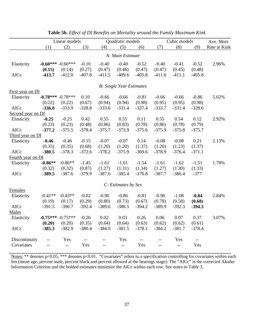
37

Table 5b. Effect of DI Benefits on Mortality around the Family Maximum Kink

Linear models Quadratic models Cubic models Ave. Mort. Rate at Kink (1) (2) (3) (4) (5) (6) (7) (8) (9)

A: Main Estimate

Elasticity -0.60*** -0.60*** -0.10 -0.40 -0.40 -0.52 -0.40 -0.41 -0.52 2.96% (0.15) (0.14) (0.27) (0.47) (0.46) (0.47) (0.47) (0.45) (0.48)

AICc -413.7 -412.0 -407.8 -411.5 -409.6 -405.8 -411.6 -411.1 -405.8 B: Single Year Estimates

First year on DI Elasticity -0.78*** -0.78*** 0.10 -0.66 -0.66 -0.81 -0.66 -0.66 -0.86 5.02%

(0.22) (0.22) (0.67) (0.94) (0.94) (0.98) (0.95) (0.95) (0.98) AICc -336.0 -333.9 -328.8 -333.6 -331.4 -327.4 -333.7 -331.4 -328.6

Second year on DI Elasticity -0.25 -0.25 0.42 0.55 0.55 0.11 0.55 0.54 0.12 2.92%

(0.23) (0.23) (0.48) (0.86) (0.83) (0.78) (0.86) (0.78) (0.79) AICc -377.2 -375.5 -378.4 -375.7 -373.9 -375.6 -375.9 -375.8 -375.7

Third year on DI Elasticity -0.46 -0.46 -0.15 -0.07 -0.07 0.14 -0.08 -0.08 0.21 2.13%

(0.35) (0.35) (0.68) (1.20) (1.20) (1.37) (1.20) (1.23) (1.37) AICc -380.5 -378.3 -372.6 -378.2 -375.9 -369.6 -378.9 -376.4 -371.1

Fourth year on DI Elasticity -0.86** -0.86** -1.45 -1.61 -1.61 -1.54 -1.61 -1.62 -1.51 1.78% (0.32) (0.32) (0.87) (1.27) (1.31) (1.34) (1.27) (1.30) (1.33) AICc -389.5 -387.6 -379.9 -387.6 -385.4 -376.8 -387.7 -386.4 -377 C: Estimates by Sex

Females Elasticity -0.41** -0.43** -0.02 -0.90 -0.86 -0.81 -0.96 -1.08 -0.84 2.84%

(0.19) (0.17) (0.29) (0.80) (0.73) (0.67) (0.78) (0.58) (0.68) AICc -391.5 -390.7 -392.4 -389.6 -388.5 -394.2 -389.9 -392.3 -394.3

Males Elasticity -0.75*** -0.75*** -0.26 0.02 0.03 0.26 0.06 0.07 0.37 3.07%

(0.20) (0.20) (0.35) (0.64) (0.64) (0.63) (0.62) (0.62) (0.61) AICc -385.3 -382.9 -380.4 -384.0 -381.5 -378.1 -384.2 -381.7 -378.4 Discontinuity -- Yes -- -- Yes -- -- Yes -- Covariates -- -- Yes -- -- Yes -- -- Yes Notes: ** denotes p<0.05, *** denotes p<0.01. “Covariates” refers to a specification controlling for covariates within each bin (mean age, percent male, percent black and percent allowed at the hearings stage). The “AICc” is the corrected Akaike Information Criterion and the bolded estimates minimize the AICc within each row. See notes to Table 3.

38

Table 5c. Effect of DI Benefits on Mortality around the Upper Kink

Linear models Quadratic models Cubic models Ave. Mort. Rate at Kink (1) (2) (3) (4) (5) (6) (7) (8) (9)

A: Main Estimate

Elasticity 0.47*** 0.43*** -0.02 -0.29 -0.21 0.07 -0.04 -0.09 0.07 4.79% (0.10) (0.09) (0.21) (0.39) (0.34) (0.41) (0.39) (0.38) (0.41)

AICc -704.3 -707.9 -708.8 -708.8 -711.3 -708.9 -713.7 -712.5 -709.7 B: Single Year Estimates

First year on DI Elasticity 0.28 0.20 0.09 0.43 0.58 0.70 0.88 0.76 0.70 8.14%

(0.19) (0.18) (0.39) (0.82) (0.72) (0.77) (0.77) (0.77) (0.76) AICc -574.7 -578.3 -576.2 -574.8 -578.7 -577.2 -579.8 -579.5 -579.5

Second year on DI Elasticity 0.62*** 0.64*** 0.23 -0.44 -0.50 -0.78 -0.35 -0.20 -0.77 4.54%

(0.21) (0.21) (0.46) (0.66) (0.69) (0.95) (0.79) (0.78) (0.95) AICc -621.4 -619.5 -615.5 -623.3 -621.7 -617.1 -623.4 -623.1 -617.3

Third year on DI Elasticity 0.71** 0.69** -0.09 -1.21 -1.21 0.27 -1.04 -0.97 0.27 3.48%

(0.30) (0.30) (0.65) (1.25) (1.30) (1.33) (1.32) (1.28) (1.34) AICc -620.2 -618.1 -624.9 -623.8 -621.6 -625.1 -624.1 -622.1 -625.2

Fourth year on DI Elasticity 0.51 0.41 -0.61 -0.94 -0.79 -0.59 -0.92 -1.22 -0.60 3.01% (0.28) (0.28) (0.71) (1.26) (1.18) (1.54) (1.35) (1.24) (1.54) AICc -621.8 -622 -617.5 -623.4 -623.1 -617.5 -623.4 -624.4 -617.8 C: Estimates by Sex

Females Elasticity -0.25 -0.36 -0.53 -0.74 -0.58 -0.38 -0.12 -0.23 -0.10 4.23%

(0.19) (0.19) (0.28) (0.66) (0.69) (0.71) (0.75) (0.75) (0.81) AICc -646.5 -647.4 -652.8 -647.0 -647.6 -652.8 -650.2 -648.5 -653.7

Males Elasticity 0.80*** 0.76*** 0.13 -0.21 -0.16 -0.05 0.00 -0.02 0.00 5.01%

(0.12) (0.12) (0.30) (0.49) (0.44) (0.54) (0.50) (0.49) (0.55) AICc -673.3 -675 -674.5 -678.5 -679.6 -674.7 -682.9 -681 -677.2 Discontinuity -- Yes -- -- Yes -- -- Yes -- Covariates -- -- Yes -- -- Yes -- -- Yes Notes: ** denotes p<0.05, *** denotes p<0.01. “Covariates” refers to a specification controlling for covariates within each bin (mean age, percent male, percent black and percent allowed at the hearings stage). The “AICc” is the corrected Akaike Information Criterion and the bolded estimates minimize the AICc within each row. See notes to Table 3.

39

Table 6. Placebo Mortality Tests

Linear models Quadratic models Cubic models Ave. Mort. Rate at Kink (1) (2) (4) (5) (7) (8)

A: Family Maximum Kink using Beneficiaries without Dependents

Elasticity -0.14** -0.14** -0.07 -0.07 -0.07 -0.07 4.11% (0.06) (0.06) (0.25) (0.25) (0.25) (0.26)

AIC -447.0 -445.5 -447.1 -445.6 -448.5 -446.2

B: Lower Kink using Non-beneficiaries

Elasticity 0.08 0.13 0.32 0.22 0.02 0.09 0.25% (0.50) (0.50) (1.73) (2.05) (1.90) (1.98)

AIC -268.3 -266.0 -268.3 -266.0 -265.9 -262.9

C: Family Maximum Kink using Non-beneficiaries

Elasticity 0.71 0.72 1.95 1.93 1.99 2.03 0.24% (0.46) (0.45) (2.03) (2.02) (2.06) (1.99)

AIC -499.5 -497.6 -500.0 -498.0 -500.2 -499.7

D: Upper Kink based using Non-beneficiaries

Elasticity -0.36 -0.41 3.48 3.61 3.29 2.94 0.23% (0.91) (0.94) (3.37) (3.37) (3.66) (3.61)

AIC -811.2 -809.0 -812.6 -810.6 -812.7 -811.1 Discontinuity -- Yes -- Yes -- Yes

Notes: ** denotes p<0.05, *** denotes p<0.01. Panel A estimates come from a sample of 1,066,679 DI beneficiaries without dependents that are within $900 of the family maximum kink. Data sources and sample restrictions are the same as the other samples used in the paper. The other estimates come from samples drawn from the 2009 Continuous Work History Sample, which is a1% sample of active SSNs linked to the Master Beneficiary Record and Numident files. We focus on fully-insured workers aged 18-57 years who did not have a previous DI entitlement and calculate AIME based on previous earnings (all of this is evaluated as at January 1st, 2005). Mortality is measured from 2006 to 2009. The same bandwidths are used for each of the non-beneficiary samples, and the numbers of observations are 203,656 (around lower bend point), 377,150 (around family maximum kink) and 499,482 (around upper bend point). “Covariates” refers to a specification controlling for covariates within each bin (mean age, percent male, percent black and percent allowed at the hearings stage). The “AICc” is the corrected Akaike Information Criterion and the bolded estimates minimize the AICc within each row. See notes to Table 3.

40

Table 7a. Robustness of the Mortality Effects around the Lower Bend Point

Linear models Quadratic models Cubic models (1) (2) (3) (4) (5) (6) (7) (8) (9)

Main estimate Elasticity -0.41*** -0.40*** -0.56* -0.91*** -0.94*** -0.95** -1.11*** -1.13*** -1.05**

(0.10) (0.11) (0.31) (0.29) (0.28) (0.42) (0.33) (0.37) (0.46) AIC -226.9 -224.2 -215.8 -227.3 -224.7 -214.3 -230.5 -227.5 -215.4

Using a grouped logit model Elasticity -0.37*** -0.36*** -0.52 -0.87*** -0.90*** -0.91** -1.07*** -1.08*** -0.99**

(0.09) (0.10) (0.30) (0.29) (0.27) (0.39) (0.31) (0.34) (0.43) AIC -94.6 -92.0 -83.9 -95.4 -93.1 -83.0 -98.9 -95.8 -83.9

Sample change 1 – including SSI recipients Elasticity 0.20** 0.21** -0.21 -0.55** -0.58** -0.30** -0.67*** -0.67*** -0.36

(0.09) (0.09) (0.14) (0.19) (0.21) (0.13) (0.11) (0.11) (0.18) AIC -239.2 -238.6 -256.9 -247.3 -250.1 -258.9 -265.5 -262.3 -254.2

Sample change 2 – including beneficiaries with more than four AIME changes Elasticity -0.35*** -0.34*** -0.57 -0.91*** -0.94*** -1.01** -1.14*** -1.16*** -1.12**

(0.10) (0.11) (0.28) (0.28) (0.26) (0.39) (0.29) (0.34) (0.43) AIC -227.6 -225.0 -218.1 -229.1 -227.0 -217.8 -234.0 -231.1 -218.7

Using individual-level data (with main sample) Elasticity -0.41*** -0.40*** -0.17** -0.89*** -0.92*** -0.85*** -1.14*** -1.17*** -1.10***

(0.07) (0.07) (0.06) (0.23) (0.23) (0.22) (0.26) (0.26) (0.25) AIC -1,029,822

-1,029,821 -1,060,013

-1,029,825 -1,029,824

-1,060,021 -1,029,831

-1,029,830 -1,060,028

Using $25 bins (with main sample) Elasticity -0.41*** -0.40*** -0.45** -0.94*** -0.97*** -1.10*** -1.16*** -1.18*** -1.22***

(0.08) (0.09) (0.18) (0.24) (0.23) (0.29) (0.27) (0.30) (0.32) AIC -443.7 -441.5 -435.2 -446.1 -444.5 -441.7 -450.7 -448.5 -443.6

Using $100 bins (with main sample) Elasticity -0.42*** -0.42*** -1.36*** -0.91*** -0.93** -1.36** -1.09*** -1.12*** -1.53***

(0.09) (0.11) (0.20) (0.24) (0.30) (0.23) (0.23) (0.19) (0.01) AIC -120.8 -116.6 -107.7 -121.4 -116.0 -78.7 -127.4 -122.7 -178.9

Discontinuity -- Yes -- -- Yes -- -- Yes -- Covariates -- -- Yes -- -- Yes -- -- Yes Notes: ** denotes p<0.05, *** denotes p<0.01. We re-present the main results and six more sets of results. First is from a grouped logit model, where the dependent variable is ln[mortality rate/(1 – mortality rate)] and the coefficients are transformed into marginal effects by multiplying them by E[(mortality rate)/(1 – mortality rate)]. Second and third are sample changes using the main specification: including SSI recipients and then including beneficiaries with more than four AIME changes. Fourth, fifth and sixth use the main sample and change the level of aggregation: using the individual level, smaller $25 bins and larger $100 bins. “Covariates” refers to a specification controlling for covariates within each bin (mean age, percent male, percent black and percent allowed at the hearings stage). The “AICc” is the corrected Akaike Information Criterion and the bolded estimates minimize the AICc within each row. See notes to Table 3 for more details.

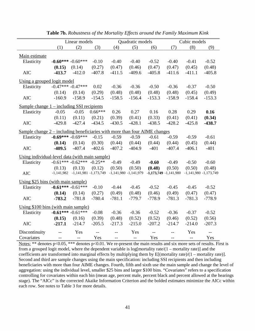
41

Table 7b. Robustness of the Mortality Effects around the Family Maximum Kink

Linear models Quadratic models Cubic models (1) (2) (3) (4) (5) (6) (7) (8) (9)

Main estimate Elasticity -0.60*** -0.60*** -0.10 -0.40 -0.40 -0.52 -0.40 -0.41 -0.52

(0.15) (0.14) (0.27) (0.47) (0.46) (0.47) (0.47) (0.45) (0.48) AIC -413.7 -412.0 -407.8 -411.5 -409.6 -405.8 -411.6 -411.1 -405.8

Using a grouped logit model Elasticity -0.47*** -0.47*** 0.02 -0.36 -0.36 -0.50 -0.36 -0.37 -0.50

(0.14) (0.14) (0.29) (0.48) (0.48) (0.48) (0.48) (0.45) (0.49) AIC -160.9 -158.9 -154.5 -158.5 -156.4 -153.3 -158.9 -158.4 -153.3

Sample change 1 – including SSI recipients Elasticity -0.05 -0.05 0.66*** 0.26 0.27 0.16 0.28 0.29 0.16

(0.11) (0.11) (0.21) (0.39) (0.41) (0.33) (0.41) (0.41) (0.34) AIC -429.8 -427.4 -434.5 -430.5 -428.1 -438.5 -428.2 -425.8 -438.7

Sample change 2 – including beneficiaries with more than four AIME changes Elasticity -0.69*** -0.69*** -0.15 -0.59 -0.59 -0.61 -0.59 -0.59 -0.61

(0.14) (0.14) (0.30) (0.44) (0.44) (0.44) (0.44) (0.45) (0.44) AIC -409.5 -407.4 -402.6 -407.2 -404.9 -401 -407.4 -406.1 -401

Using individual-level data (with main sample) Elasticity -0.61*** -0.62*** -0.25** -0.49 -0.49 -0.60 -0.49 -0.50 -0.60

(0.13) (0.13) (0.12) (0.50) (0.50) (0.48) (0.50) (0.50) (0.48) AIC -1,141,982 -1,141,981 -1,173,749 -1,141,980 -1,141,979 -1,173,749 -1,141,980 -1,141,980 -1,173,749

Using $25 bins (with main sample) Elasticity -0.61*** -0.61*** -0.10 -0.44 -0.45 -0.52 -0.45 -0.45 -0.52

(0.14) (0.14) (0.27) (0.49) (0.48) (0.46) (0.49) (0.47) (0.47) AIC -783.2 -781.8 -780.4 -781.1 -779.7 -778.9 -781.3 -781.3 -778.9

Using $100 bins (with main sample) Elasticity -0.61*** -0.61*** -0.08 -0.36 -0.36 -0.52 -0.36 -0.37 -0.52

(0.15) (0.16) (0.39) (0.48) (0.52) (0.52) (0.46) (0.52) (0.56) AIC -217.1 -214.7 -205.5 -217.3 -215.0 -207.2 -214.7 -214.0 -207.3

Discontinuity -- Yes -- -- Yes -- -- Yes -- Covariates -- -- Yes -- -- Yes -- -- Yes Notes: ** denotes p<0.05, *** denotes p<0.01. We re-present the main results and six more sets of results. First is from a grouped logit model, where the dependent variable is log[mortality rate/(1 – mortality rate)] and the coefficients are transformed into marginal effects by multiplying them by E[(mortality rate)/(1 – mortality rate)]. Second and third are sample changes using the main specification: including SSI recipients and then including beneficiaries with more than four AIME changes. Fourth, fifth and sixth use the main sample and change the level of aggregation: using the individual level, smaller $25 bins and larger $100 bins. “Covariates” refers to a specification controlling for covariates within each bin (mean age, percent male, percent black and percent allowed at the hearings stage). The “AICc” is the corrected Akaike Information Criterion and the bolded estimates minimize the AICc within each row. See notes to Table 3 for more details.

42

Table 8a. Heterogeneity in the Mortality Effects around the Lower Bend Point

Category

Subgroup p.p. change per

$1,000 more in DI Elasticity Mortality rate

at kink (1) (2) (3) All -0.47*** -1.11*** 3.61% (0.14) (0.33) Age at filing for DI Age < 45 years -0.45** -1.85** 2.06% (0.16) (0.65) Age ≥ 45 years -0.47** -0.91** 4.42% (0.17) (0.32) Race Nonblack -0.43*** -1.03*** 3.58%

(0.14) (0.34) Black -0.82** -1.84** 3.84%

(0.37) (0.83) Type of allowance Initial DDS allowance -0.66*** -1.18*** 4.74%

(0.18) (0.32) Hearings allowance -0.03 -0.20 1.24% (0.11) (0.76) When entered DI Started in 1997-2005 -0.46** -0.90** 4.40% (0.16) (0.32) Started in 2006-2009 -0.39** -1.25** 2.69% (0.18) (0.56) Primary disability Mental disorders -0.30* -2.52* 1.02% (0.15) (1.25) Musculoskeletal cond. -0.06 -0.52 0.99% (0.09) (0.77) Circulatory conditions -0.70* -1.48* 4.04% (0.33) (0.71) Cancers -1.29** -0.63** 17.54% (0.60) (0.29) All other disabilities -0.34 -0.84 3.47% (0.20) (0.49)

Notes: * denotes p<0.10, ** denotes p<0.05, *** denotes p<0.01. Each estimate comes from the specification using a cubic polynomial without a discontinuity and covariates (as this is the specification that minimizes the corrected Akaike Information Criteria (AICc) for the main results). Bolded estimates are the ones for which this specification also minimizes the AICc for that subsample. Column (1) shows the coefficients (and standard errors) as percentage point changes in the annual mortality rate and scaled by a $1,000 change in annual DI payments (for ease of reading the coefficients). Column (2) shows the results as elasticities with respect to DI payments. Column (3) shows the annual mortality rates at the kink. See notes to Table 3 for more information.

43

Table 8b. Heterogeneity in the Mortality Effects around the Family Maximum Kink

Category

Subgroup p.p. change per

$1,000 more in DI Elasticity Mortality rate

at kink (1) (2) (3) All -0.09*** -0.60*** 2.96% (0.02) (0.15) Age at filing for DI Age < 45 years -0.07*** -0.64*** 2.15% (0.02) (0.21) Age ≥ 45 years -0.04 -0.19 4.47% (0.05) (0.20) Race Nonblack -0.10*** -0.68*** 2.91%

(0.02) (0.14) Black -0.06 -0.35 3.23%

(0.06) (0.33) Type of allowance Initial DDS allowance -0.13*** -0.60*** 4.07%

(0.03) (0.15) Hearings allowance 0.00 0.08 1.03% (0.02) (0.28) When entered DI Started in 1997-2005 -0.08*** -0.48*** 3.03% (0.03) (0.17) Started in 2006-2009 -0.13*** -0.84*** 2.85% (0.03) (0.21) Primary disability Mental disorders -0.02 -0.41 0.81% (0.02) (0.41) Musculoskeletal cond. 0.02 0.43 0.88% (0.02) (0.51) Circulatory conditions -0.11* -0.62* 3.37% (0.06) (0.32) Cancers -0.20*** -0.22*** 16.91% (0.07) (0.08) All other disabilities -0.07 -0.51 2.65% (0.05) (0.34)

Notes: * denotes p<0.10, ** denotes p<0.05, *** denotes p<0.01. Each estimate comes from the specification using a cubic polynomial without a discontinuity and covariates (as this is the specification that minimizes the corrected Akaike Information Criteria (AICc) for the main results). Bolded estimates are the ones for which this specification also minimizes the AICc for that subsample. Column (1) shows the coefficients (and standard errors) as percentage point changes in the annual mortality rate and scaled by a $1,000 change in annual DI payments (for ease of reading the coefficients). Column (2) shows the results as elasticities with respect to DI payments. Column (3) shows the annual mortality rates at the kink. See notes to Table 3 for more information.

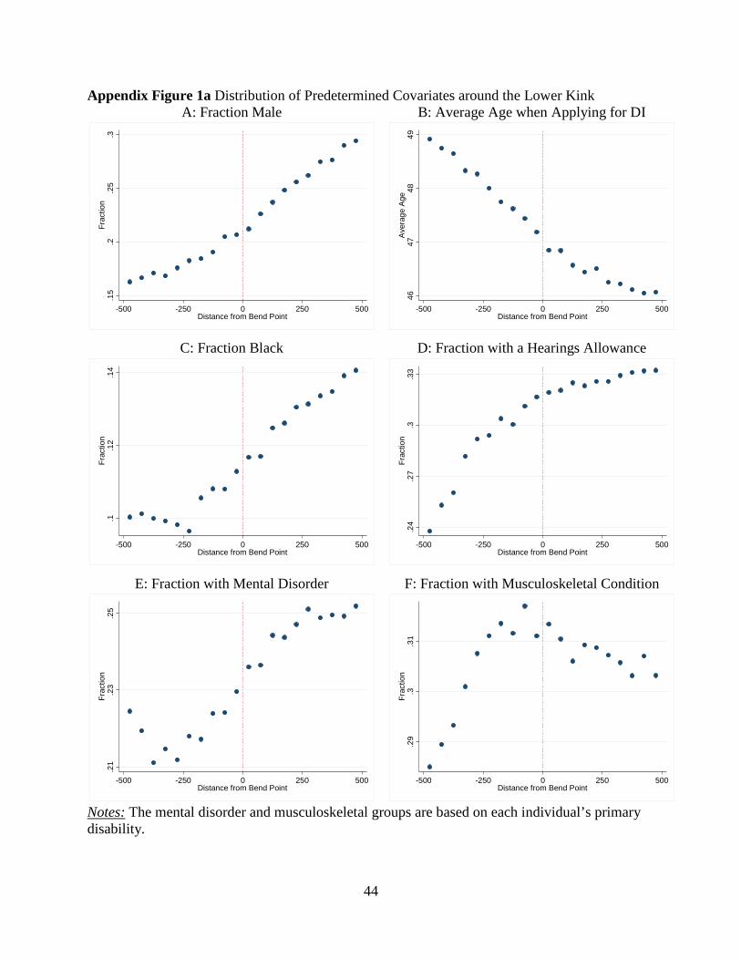
44

Appendix Figure 1a Distribution of Predetermined Covariates around the Lower Kink A: Fraction Male

C: Fraction Black

E: Fraction with Mental Disorder

B: Average Age when Applying for DI

D: Fraction with a Hearings Allowance

F: Fraction with Musculoskeletal Condition

Notes: The mental disorder and musculoskeletal groups are based on each individual’s primary disability.

.15

.2.2

5.3

Frac

tion

-500 -250 0 250 500Distance from Bend Point

.1.1

2.1

4Fr

actio

n

-500 -250 0 250 500Distance from Bend Point

.21

.23

.25

Frac

tion

-500 -250 0 250 500Distance from Bend Point

4647

4849

Ave

rage

Age

-500 -250 0 250 500Distance from Bend Point

.24

.27

.3.3

3Fr

actio

n

-500 -250 0 250 500Distance from Bend Point

.29

.3.3

1Fr

actio

n

-500 -250 0 250 500Distance from Bend Point

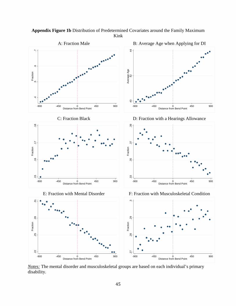
45

Appendix Figure 1b Distribution of Predetermined Covariates around the Family Maximum Kink

A: Fraction Male

C: Fraction Black

E: Fraction with Mental Disorder

B: Average Age when Applying for DI

D: Fraction with a Hearings Allowance

F: Fraction with Musculoskeletal Condition

Notes: The mental disorder and musculoskeletal groups are based on each individual’s primary disability.

.4.5

.6.7

Frac

tion

-900 -450 0 450 900Distance from Bend Point

.15

.16

.17

.18

Frac

tion

-900 -450 0 450 900Distance from Bend Point

.22

.25

.28

.31

Frac

tion

-900 -450 0 450 900Distance from Bend Point

4042

44A

vera

ge A

ge

-900 -450 0 450 900Distance from Bend Point

.33

.35

.37

.39

Frac

tion

-900 -450 0 450 900Distance from Bend Point

.27

.28

.29

.3Fr

actio

n

-900 -450 0 450 900Distance from Bend Point

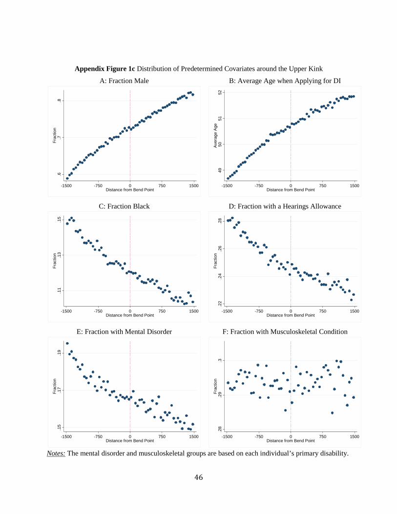
46

Appendix Figure 1c Distribution of Predetermined Covariates around the Upper Kink

A: Fraction Male

C: Fraction Black

E: Fraction with Mental Disorder

B: Average Age when Applying for DI

D: Fraction with a Hearings Allowance

F: Fraction with Musculoskeletal Condition

Notes: The mental disorder and musculoskeletal groups are based on each individual’s primary disability.

.6.7

.8Fr

actio

n

-1500 -750 0 750 1500Distance from Bend Point

.11

.13

.15

Frac

tion

-1500 -750 0 750 1500Distance from Bend Point

.15

.17

.19

Frac

tion

-1500 -750 0 750 1500Distance from Bend Point

4950

5152

Ave

rage

Age

-1500 -750 0 750 1500Distance from Bend Point

.22

.24

.26

.28

Frac

tion

-1500 -750 0 750 1500Distance from Bend Point

.28

.29

.3Fr

actio

n

-1500 -750 0 750 1500Distance from Bend Point

47

Appendix Figure 2 Distribution of Primary Insurance Amount/Family Payments

A: Primary Insurance Amount around Lower Kink

B: Primary Insurance Amount around Upper Kink

250

500

750

Prim

ary

Insu

ranc

e A

mou

nt ($

)

-500 -250 0 250 500Distance from Bend Point

1500

1750

2000

Prim

ary

Insu

ranc

e A

mou

nt ($

)

-1500 -750 0 750 1500Distance from Bend Point

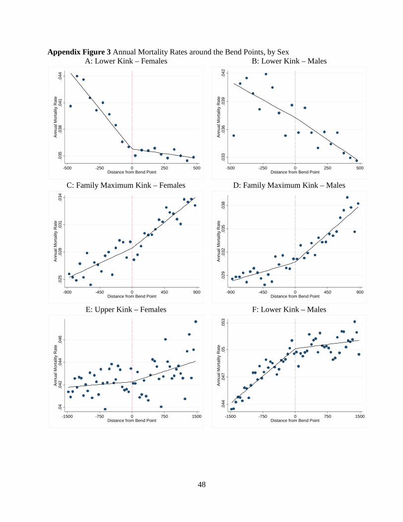
48

Appendix Figure 3 Annual Mortality Rates around the Bend Points, by SexA: Lower Kink – Females

C: Family Maximum Kink – Females

E: Upper Kink – Females

B: Lower Kink – Males

D: Family Maximum Kink – Males

F: Lower Kink – Males

.035

.038

.041

.044

Ann

ual M

orta

lity

Rat

e

-500 -250 0 250 500Distance from Bend Point

.025

.028

.031

.034

Ann

ual M

orta

lity

Rat

e

-900 -450 0 450 900Distance from Bend Point

.04

.042

.044

.046

Ann

ual M

orta

lity

Rat

e

-1500 -750 0 750 1500Distance from Bend Point

.033

.036

.039

.042

Ann

ual M

orta

lity

Rat

e

-500 -250 0 250 500Distance from Bend Point

.029

.032

.035

.038

Ann

ual M

orta

lity

Rat

e

-900 -450 0 450 900Distance from Bend Point

.044

.047

.05

.053

Ann

ual M

orta

lity

Rat

e

-1500 -750 0 750 1500Distance from Bend Point

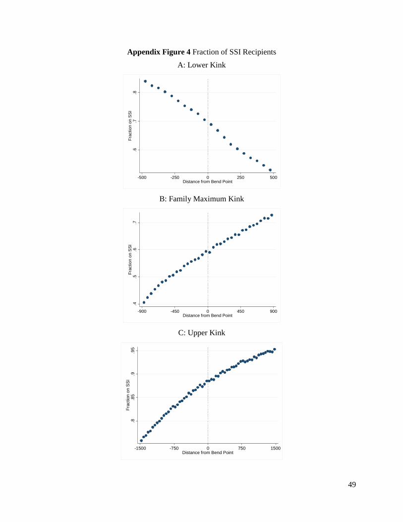
49

Appendix Figure 4 Fraction of SSI Recipients

A: Lower Kink

B: Family Maximum Kink

C: Upper Kink

.6.7

.8Fr

actio

n on

SSI

-500 -250 0 250 500Distance from Bend Point

.4.5

.6.7

Frac

tion

on S

SI

-900 -450 0 450 900Distance from Bend Point

.8.8

5.9

.95

Frac

tion

on S

SI

-1500 -750 0 750 1500Distance from Bend Point

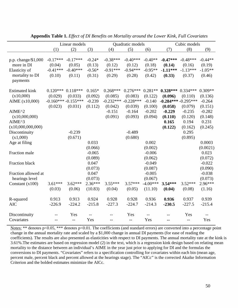
50

Appendix Table 1. Effect of DI Benefits on Mortality around the Lower Kink, Full Covariates

Linear models Quadratic models Cubic models (1) (2) (3) (4) (5) (6) (7) (8) (9)

p.p. change/$1,000

more in DI -0.17*** -0.17*** -0.24* -0.38*** -0.40*** -0.40** -0.47*** -0.48*** -0.44**

(0.04) (0.05) (0.13) (0.12) (0.12) (0.18) (0.14) (0.16) (0.19) Elasticity of

mortality to DI payments

-0.41*** -0.40*** -0.56* -0.91*** -0.94*** -0.95** -1.11*** -1.13*** -1.05** (0.10) (0.11) (0.31) (0.29) (0.28) (0.42) (0.33) (0.37) (0.46)

Estimated kink

(x10,000) 0.120*** 0.118*** 0.165* 0.268*** 0.276*** 0.281** 0.328*** 0.334*** 0.309** (0.029) (0.033) (0.092) (0.085) (0.083) (0.122) (0.096) (0.110) (0.136)

AIME (x10,000) -0.160*** -0.155*** -0.239 -0.232*** -0.228*** -0.140 -0.284*** -0.295*** -0.264 (0.023) (0.031) (0.112) (0.042) (0.039) (0.100) (0.058) (0.079) (0.151) AIME^2 -0.151 -0.164 -0.202 -0.229 -0.235 -0.282

(x10,000,000) (0.091) (0.093) (0.094) (0.110) (0.120) (0.148) AIME^3 (x10,000,000,000)

0.165 0.194 0.231 (0.122) (0.162) (0.245)

Discontinuity -0.239 -0.489 0.295 (x1,000) (0.671) (0.680) (0.895)

Age at filing 0.033 0.002 0.0003 (0.066) (0.002) (0.0021)

Fraction male -0.065 -0.006 0.023 (0.089) (0.062) (0.072) Fraction black 0.047 -0.049 -0.022 (0.073) (0.087) (0.090) Fraction allowed at

hearings level 0.047 -0.005 -0.038 (0.073) (0.067) (0.073)

Constant (x100) 3.61*** 3.62*** 2.36*** 3.55*** 3.57*** -4.00*** 3.54*** 3.52*** 2.96*** (0.03) (0.06) (10.83) (0.04) (0.05) (11.10) (0.04) (0.08) (1.16) R-squared 0.913 0.913 0.924 0.928 0.928 0.936 0.936 0.937 0.939 AIC -226.9 -224.2 -215.8 -227.3 -224.7 -214.3 -230.5 -227.5 -215.4 Discontinuity -- Yes -- -- Yes -- -- Yes -- Covariates -- -- Yes -- -- Yes -- -- Yes

Notes: ** denotes p<0.05, *** denotes p<0.01. The coefficients (and standard errors) are converted into a percentage point change in the annual mortality rate and scaled by a $1,000 change in annual DI payments (for ease of reading the coefficients). The results are also presented as elasticities with respect to DI payments. The annual mortality rate at the kink is 3.61%.The estimates are based on regression model (2) in the text, which is a regression kink design based on relating mean mortality to the distance between an individual’s AIME in the year just prior to applying for DI and the formulas the conversions to DI payments. “Covariates” refers to a specification controlling for covariates within each bin (mean age, percent male, percent black and percent allowed at the hearings stage). The “AICc” is the corrected Akaike Information Criterion and the bolded estimates minimize the AICc.

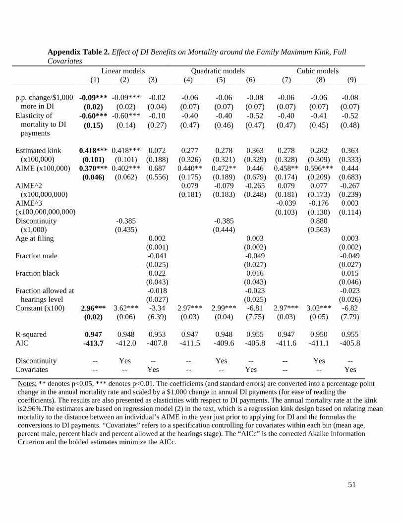
51

Appendix Table 2. Effect of DI Benefits on Mortality around the Family Maximum Kink, Full Covariates

Linear models Quadratic models Cubic models (1) (2) (3) (4) (5) (6) (7) (8) (9)

p.p. change/$1,000

more in DI -0.09*** -0.09*** -0.02 -0.06 -0.06 -0.08 -0.06 -0.06 -0.08

(0.02) (0.02) (0.04) (0.07) (0.07) (0.07) (0.07) (0.07) (0.07) Elasticity of

mortality to DI payments

-0.60*** -0.60*** -0.10 -0.40 -0.40 -0.52 -0.40 -0.41 -0.52 (0.15) (0.14) (0.27) (0.47) (0.46) (0.47) (0.47) (0.45) (0.48)

Estimated kink

(x100,000) 0.418*** 0.418*** 0.072 0.277 0.278 0.363 0.278 0.282 0.363 (0.101) (0.101) (0.188) (0.326) (0.321) (0.329) (0.328) (0.309) (0.333)

AIME (x100,000) 0.370*** 0.402*** 0.687 0.440** 0.472** 0.446 0.458** 0.596*** 0.444 (0.046) (0.062) (0.556) (0.175) (0.189) (0.679) (0.174) (0.209) (0.683) AIME^2 0.079 -0.079 -0.265 0.079 0.077 -0.267

(x100,000,000) (0.181) (0.183) (0.248) (0.181) (0.173) (0.239) AIME^3 (x100,000,000,000)

-0.039 -0.176 0.003 (0.103) (0.130) (0.114)

Discontinuity -0.385 -0.385 0.880 (x1,000) (0.435) (0.444) (0.563)

Age at filing 0.002 0.003 0.003 (0.001) (0.002) (0.002)

Fraction male -0.041 -0.049 -0.049 (0.025) (0.027) (0.027) Fraction black 0.022 0.016 0.015 (0.043) (0.043) (0.046) Fraction allowed at

hearings level -0.018 -0.023 -0.023 (0.027) (0.025) (0.026)

Constant (x100) 2.96*** 3.62*** -3.34 2.97*** 2.99*** -6.81 2.97*** 3.02*** -6.82 (0.02) (0.06) (6.39) (0.03) (0.04) (7.75) (0.03) (0.05) (7.79) R-squared 0.947 0.948 0.953 0.947 0.948 0.955 0.947 0.950 0.955 AIC -413.7 -412.0 -407.8 -411.5 -409.6 -405.8 -411.6 -411.1 -405.8 Discontinuity -- Yes -- -- Yes -- -- Yes -- Covariates -- -- Yes -- -- Yes -- -- Yes

Notes: ** denotes p<0.05, *** denotes p<0.01. The coefficients (and standard errors) are converted into a percentage point change in the annual mortality rate and scaled by a $1,000 change in annual DI payments (for ease of reading the coefficients). The results are also presented as elasticities with respect to DI payments. The annual mortality rate at the kink is2.96%.The estimates are based on regression model (2) in the text, which is a regression kink design based on relating mean mortality to the distance between an individual’s AIME in the year just prior to applying for DI and the formulas the conversions to DI payments. “Covariates” refers to a specification controlling for covariates within each bin (mean age, percent male, percent black and percent allowed at the hearings stage). The “AICc” is the corrected Akaike Information Criterion and the bolded estimates minimize the AICc.