RESEARCH ARTICLE

The effect of acquisition error and level of detail on the accuracy of spatialanalysesFilip Biljecki a, Gerard B.M. Heuvelink b, Hugo Ledoux a and Jantien Stoter a

a3D Geoinformation, Delft University of Technology, Netherlands; bSoil Geography and Landscape group, Wageningen University,Netherlands

ABSTRACTThere has been a great deal of research about errors in geographic information and how theyaffect spatial analyses. A typical GIS process introduces various types of errors at different stages,and such errors usually propagate into errors in the result of a spatial analysis. However, moststudies consider only a single error type thus preventing the understanding of the interaction andrelative contributions of different types of errors. We focus on the level of detail (LOD) andpositional error, and perform a multiple error propagation analysis combining both types of error.We experiment with three spatial analyses (computing gross volume, envelope area, and solarirradiation of buildings) performed with procedurally generated 3D city models to decouple anddemonstrate the magnitude of the two types of error, and to show how they individually andjointly propagate to the output of the employed spatial analysis. The most notable result is that inthe considered spatial analyses the positional error has a much higher impact than the LOD. As aconsequence, we suggest that it is pointless to acquire geoinformation of a fine LOD if theacquisition method is not accurate, and instead we advise focusing on the accuracy of the data.

ARTICLE HISTORYReceived 06 October 2016Accepted 05 January 2017

KEYWORDSScale; level of detail; error;accuracy; 3D city model;CityGML

Introduction

Geographical data are produced in many different fla-vors and combinations: at different levels of detail(LODs) and at different accuracies depending on thenature of the data, spatial scale, acquisition technique,and available funds. These different qualities affectspatial analyses in distinct ways, and investigating thepropagation of a specific type of error (e.g. thematicerror) has been extensively researched in geographicalinformation science. However, mixed error propaga-tion studies, which analyze the joint propagation ofmultiple error types, are scarce. Error propagationanalyses commonly focus on one type of error and onone spatial analysis, and they are never carried out atmultiple scales. This prevents the understanding of therelation, magnitude and relative contribution of eachtype of error.

In this paper we focus on the errors induced by (i)different LODs and by (ii) positional errors incurred bythe acquisition. We run experiments to isolate andquantify them, and to investigate whether the benefitprovided by spatial data of finer LOD is still valid incases of significant acquisition errors.

Understanding the relation between detail and acqui-sition error is important for stakeholders in GIScience in

order to put the two quality characteristics into perspec-tive. For example, the presented approach provides prac-titioners and scientists a way of determining whether it isworth increasing the accuracy of the dataset, or rather itsLOD, when designing the specification of a dataset to beacquired, so that the produced data will be suitable for aspecific purpose (e.g. “What should the minimum accu-racy and LOD available in the data be, so that these areusable for accurately calculating the volume of build-ings?”). Likewise, it is relevant to set expectations aboutthe capabilities of a certain dataset: this involves deter-mining whether a dataset is adequately detailed andaccurate enough to derive sufficiently reliable results ina spatial analysis. For instance, a user can avoid orderingthe acquisition of an expensive and overly detailed data-set, which in a certain spatial analysis brings only aminuscule benefit when compared with a less detailedand less costly alternative.

Before proceeding to the core of the paper, it is impor-tant to separate the two considered qualities of geogra-phical data – LOD and accuracy, which are unfortunatelyperennially misapprehended as synonyms. While there isan association between the two (representations at finerscales tend to be of higher quality (Heuvelink, 1998)),these are two independent concepts (Chrisman, 1991).

CONTACT Filip Biljecki f.biljecki@tudelft.nl

CARTOGRAPHY AND GEOGRAPHIC INFORMATION SCIENCE, 2018VOL. 45, NO. 2, 156–176https://doi.org/10.1080/15230406.2017.1279986

© 2017 The Author(s). Published by Informa UK Limited, trading as Taylor & Francis GroupThis is an Open Access article distributed under the terms of the Creative Commons Attribution-NonCommercial-NoDerivatives License (http://creativecommons.org/licenses/by-nc-nd/4.0/), which permits non-commercial re-use, distribution, and reproduction in any medium, provided the original work is properly cited, and is not altered, transformed, or builtupon in any way.

Dow

nloa

ded

by [2

7.0.

232.

205]

at 1

9:14

19

Dec

embe

r 201

7

For instance, a national government may produce a GISdataset in which buildings are modeled in a coarse butaccurately derived representation, and a municipalitymay produce a dataset of a city in finer detail but withless accuracy due to an inferior acquisition technique (e.g.automatic reconstruction from lidar instead of terrestrialmeasurements).

While acquisition induces multiple types of errors(e.g. thematic and positional), in this paper we focus onthe positional errors resulting from acquisition.However, the developed work may be applied to inves-tigate other aspects of acquisition as well.

The type of questions that we address in this paperare usual considerations for GIS users:

• Given two distinct datasets covering the same area(from multiple sources), where one is less detailed butmore accurate than the other, which is the better choicefor a particular spatial analysis?

• At what LOD and at what accuracy should a 3Dmodel be acquired to be usable for a particular spatialanalysis? Understanding this aspect would aid dataproducers in designing a specification that bears inmind the intended use of the data.

• Is it beneficial to acquire a dataset of a fine LOD ifthe acquisition technique has poor accuracy?Understanding this aspect may prevent wasting effortto produce a dataset that is detailed and it is perhapsvisually pleasing, but is ultimately not acceptable for aparticular spatial analysis because of poor accuracy.This reasoning was also described by Burrough andMcDonnell (1998): “The quality of GIS products is

often judged by the visual appearance of the end-pro-duct [. . .]. Uncertainties and errors are intrinsic tospatial data and need to be addressed properly, notswept away under the carpet of fancy graphics dis-plays.” (p. 220)

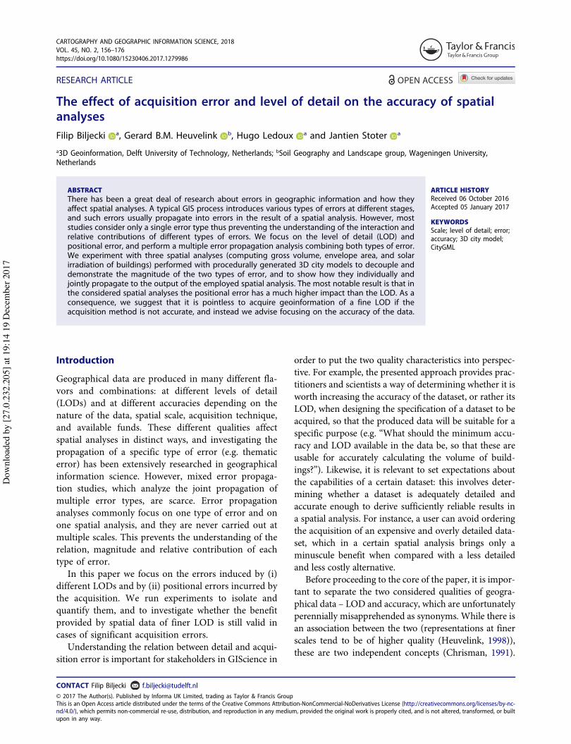
This research is also relevant in regard to theincreasing availability of datasets with heterogeneousquality (Goodchild & Li, 2012). An example of suchdataset is one based on old but accurate cadastral data,in which newer buildings have been supplemented withother acquisition techniques such as footprints digi-tized from aerial images. Such approaches may resultin data of variable accuracy and differing LODs, aphenomenon inherent to volunteered geoinformation(Camboim, Bravo, & Sluter, 2015; Fan, Zipf, Fu, &Neis, 2014; Senaratne, Mobasheri, Ali, Capineri, &Haklay, 2017; Touya & Brando-Escobar, 2013; Uden& Zipf, 2013). Because such data are becoming increas-ingly used for spatial analyses (Wendel, Murshed,Sriramulu, & Nichersu, 2016), it is worthwhile to inves-tigate for which portions of the dataset caution shouldbe exercised due to lower reliability than in other partsof the dataset. Figure 1 shows an example of suchdataset.

Our experiments help in determining which LODand accuracy are sufficiently acceptable for particularspatial analyses.

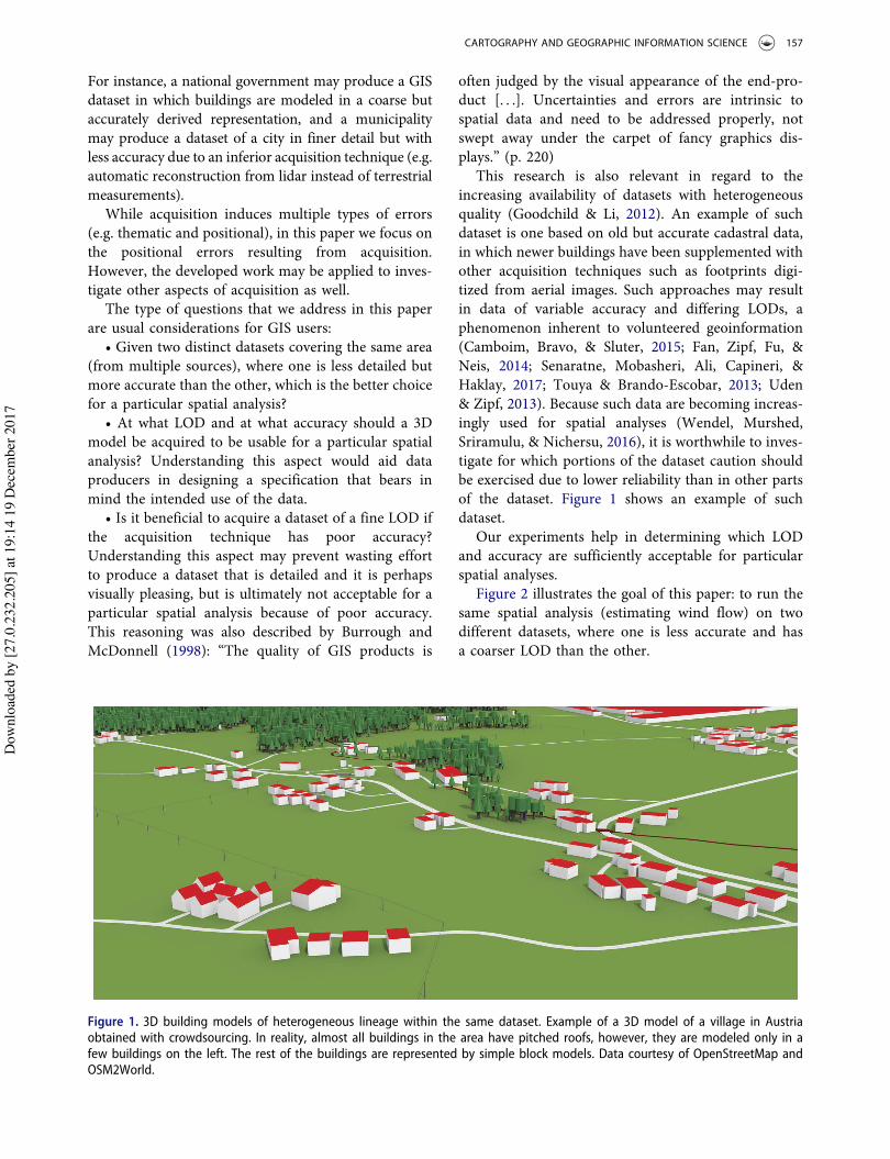
Figure 2 illustrates the goal of this paper: to run thesame spatial analysis (estimating wind flow) on twodifferent datasets, where one is less accurate and hasa coarser LOD than the other.

Figure 1. 3D building models of heterogeneous lineage within the same dataset. Example of a 3D model of a village in Austriaobtained with crowdsourcing. In reality, almost all buildings in the area have pitched roofs, however, they are modeled only in afew buildings on the left. The rest of the buildings are represented by simple block models. Data courtesy of OpenStreetMap andOSM2World.

CARTOGRAPHY AND GEOGRAPHIC INFORMATION SCIENCE 157

Dow

nloa

ded

by [2

7.0.

232.

205]

at 1

9:14

19

Dec

embe

r 201

7

While the difference between the two LODs isobvious, it cannot be determined whether the differ-ence in the results should be attributed primarily to theprogression of the LOD or to the increase in the accu-racy of the data. Furthermore, due to the absence ofground truth data, it is not clear whether the improve-ment that a more detailed dataset brings is still advan-tageous, as it may still deviate considerably from thereal-world. A minor caveat here is that due to theabsence of ground truth data we do not have proofthat in this case the dataset of the finer LOD and higheraccuracy brings more accurate results. However, it isreasonable to assume that such comparative differencesbring more accurate results (or at least equally accu-rate) in comparison to analyses using their coarser andless accurate counterparts.

In Section Background we introduce a theoreticalframework and an overview of related work. SectionData and method presents the design of a method todecompose and quantify the two types of errors underconsideration. We select three spatial analyses (estimat-ing the area of the building envelope, gross volume of abuilding, and solar irradiation of roofs) in order toinvestigate their different behaviors. We investigatewhether these spatial analyses are more sensitive topositional error or to the reduction in the LOD. Theresults are presented in Section Results and discussion.

Background: decomposition of errors andrelated work

Decoupling errors

We decompose the errors induced in a typical GISprocess into multiple components. Figure 3 illustratesour standpoint: error is induced before any acquisitionhas even taken place because a specification is designedto capture a certain subset of reality at a certain LOD.For instance, a data producer may decide to modelbuildings with simple roof shapes, without openingsand finer details; such LOD induces an error whichwe call representation-induced error.

The second step in the process is to realize the specifica-tion with data acquisition techniques. Due to the imperfec-tion of measurements, several types of errors are inducedin the process and the results of a spatial analysis arefurther degraded. When such errors propagate through aspatial analysis, we call this as acquisition-induced error.Here we focus on the positional error, as it is one of themost prominent types of errors in many context andapplication (Ariza-López & Rodríguez-Avi, 2015b;Drummond, 1995) and subject to intensive research (e.g.Biljecki, Heuvelink, Ledoux, & Stoter, 2015; Cheung & Shi,2004; Chow, Dede-Bamfo, & Dahal, 2016; Jacquez, 2012;McKenzie, Hegarty, Barrett, & Goodchild, 2016; Ruiz-Lendínez, Ariza- López, & Ureña-Cámara, 2016).

Figure 2. The results of two wind flow analyses of the Singapore central business district: one carried out on an accurate anddetailed 3D city model shown here (flow lines in blue), and another one with a crude block model (flow lines in red). The left panelshows both LODs in corresponding colors, while the right panel reveals only the data in the finer LOD for clarity. Data, analysis, andimage (c) Singapore Land Authority.

158 F. BILJECKI ET AL.

Dow

nloa

ded

by [2

7.0.

232.

205]

at 1

9:14

19

Dec

embe

r 201

7

We term the combination of the acquisition-induced and positional errors as combined error, anddescribe them in further detail in the next subsections.

Representation-induced error

Depending on the purpose and scale of measurement,real-world phenomena may be modeled in differentways – different LODs.

In appropriate scale ranges (Mackaness, 2007), datamodeled in finer detail are inherently believed to ben-efit spatial analyses, at the expense of an increased costof acquisition, storage complexity and maintenance,and hindering the speed of spatial analyses. Hence,the benefit may not always justify the investment.

Experiments that we present in this paper arerelevant for understanding how different LODsaffect the accuracy of a spatial analysis. This has atwofold meaning. First, as modeling data at finerLODs comes at a higher cost, a relevant question iswhether a certain spatial analysis can take advantageof this finer detail. Second, the problem may beapproached from the generalization perspective; 3Dgeoinformation at fine LODs may in fact be toocomplex for certain spatial analyses. Hence, thedata are occasionally generalized to reduce complex-ity while attempting to preserve usability (Deng &Cheng, 2015). Insights into the performance of theLODs may help to achieve that balance: by general-izing the models to a point at which their complexityis sufficiently reduced but at the same time theirusability is not compromised by the reduced LOD.

There has been a considerable amount of researchon the influence of different representations in

cartography and remote sensing across multiple scales(Hillsman & Rhoda, 1978). For instance, Veregin(2000) and Cheung and Shi (2004) study the effect ofthe simplification of lines (e.g. roads) in maps and theirpropagation to positional displacement.

Usery et al. (2004), Booij (2005), Chaubey, Cotter,Costello, and Soerens (2005), Ling, Ehlers, Usery, andMadden (2008), and Pogson and Smith (2015) investi-gated the effects of input rasters using different resolu-tions and found a significant difference in the outcomeof a spatial analysis. For example, the study of Chaubeyet al. (2005) indicates that the resolution of digitalelevation models affects the output of a hydrologicspatial analysis.

In another relevant study, Ruiz Arias, Tovar Pescador,Pozo Vázquez, andAlsamamra (2009) estimated the solarirradiation of several locations with digital elevationmod-els of different resolutions (100 m vs. 20m grid). A strongpoint of Ruiz Arias et al. (2009) is that predictions wereevaluated against independent, accurate measurementsfrom meteorological stations, essentially obtaining thedifference against true data. The results showed that theimprovement of the resolution of the Digital ElevationModels (DEMs) was minuscule in comparison to theerror induced by the spatial analysis.

In 3D geoinformation, the influence of differentrepresentations has mostly been evaluated in urbanplanning and related domains in which the visualimpression is the main decisive factor (Ellul &Altenbuchner, 2013; Hannibal, Brown, & Knight,2005; Herbert & Chen, 2015; Kibria, Zlatanova, Itard,& Dorst, 2009; Rautenbach, Çöltekin, & Coetzee, 2015).

There are related analyses comparing the results of aspatial analysis utilizing data of the same area modeled

Figure 3. Longitudinal error decomposition as discussed in this paper: errors are induced at different stages of a typical GIS process,most prominently errors induced by abstraction and by realization of the data. In reality it would include additional errors; see theoverview of Lunetta et al. (1991).

CARTOGRAPHY AND GEOGRAPHIC INFORMATION SCIENCE 159

Dow

nloa

ded

by [2

7.0.

232.

205]

at 1

9:14

19

Dec

embe

r 201

7

at different LODs (Besuievsky, Barroso, Beckers, &Patow, 2014; Biljecki, Ledoux, & Stoter, 2017; Billger,Thuvander, & Wästberg, 2016; Brasebin, Perret,Mustière, & Weber, 2012; Deng, Cheng, & Anumba,2016; Ellul, Adjrad, & Groves, 2016; Fai & Rafeiro,2014; Neto, 2006; Peronato, Bonjour, Stoeckli, Rey, &Andersen, 2016; Strzalka, Monien, Koukofikis, &Eicker, 2015). In general, research has demonstratedthat in certain spatial analyses the benefit of a finerLOD may be overestimated and even detrimental, asthe potential small benefit may be countervailed by costand complexity. A shortcoming of such analyses is thatmost of these are performed on only two LODs, and onreal-world data, thus preventing the focus on the repre-sentation-induced error alone. Moreover, some of thedatasets used, are generated from different sources,containing different magnitudes of errors.Furthermore, the analyses do not put the derivederror into perspective – the error induced by theLOD may seem significant, but if other errors areadded to the equation, it could turn out to beirrelevant.

An aspect that cannot be ignored is how thespatial detail is modeled, as there are multiple validrepresentations of a feature that are of the samedetail and scale. For instance, on a coarse scale acity may be represented as a point. The placement ofthe point (e.g. centroid vs. a point placed at the mostpopulous area of the city) may affect the calculationof the distance between two cities. Such examina-tions have been the subject of many research papers(Cromley, Lin, & Merwin, 2012; Hillsman & Rhoda,1978; Miller, 1996; Murray & O’Kelly, 2002). In thisresearch, we do not separate the two, but instead weuse the most common modeling approaches (e.g.median height of the roof structure is selected asthe elevation of the top surface of LOD1 models),based on the conclusions of Biljecki, Ledoux, Stoter,and Vosselman (2016).

Acquisition-induced error

The realization of the specification intrinsically intro-duces errors. Several different types of errors can beintroduced during the acquisition, which propagatethrough a spatial analysis in different ways, dependingon the context. For instance, the standard ISO 19157on geographic data quality defines several types oferrors, for example, completeness, topological, posi-tional, thematic (attribute), and temporal errors (ISO,2013). Most of these have been the focus of variousanalyses, for example, thematic error (Veregin, 1995).

In this paper we focus on positional error, which hasbeen the subject of several error propagation analyses(Beekhuizen et al., 2014; de Bruin, Heuvelink, &Brown, 2008; Heuvelink, Burrough, & Stein, 1989).For example, Goulden, Hopkinson, Jamieson, andSterling (2016) investigate the propagation of posi-tional error in point clouds to the calculation of varioustopographic attributes, such as slope, aspect, andwatershed area. Griffith, Millones, Vincent, Johnson,and Hunt (2007) and Zandbergen, Hart, Lenzer, andCamponovo (2012) observe the influence of positionalerror in geocoded addresses on various administrativeuse cases such as the assignment of houses to censusblocks, and allocation of students to their nearest pub-lic schools. Hartzell, Gadomski, Glennie, Finnegan, andDeems (2015) estimate the propagation of positionalerror from terrestrial laser scanning to the measure-ment of snow volume.

Positional errors are omnipresent in GIS and theyhave been much discussed in the literature, hence theydo not require a lengthier introduction.

Multiple error propagation analyses

Virtually all error propagation analyses focus on onetype of error. In contrast, our analysis considers twotypes of errors. To the extent of our knowledge, we areaware of only a few analyses that investigate multipletypes of errors, that is, multiple error propagationanalyses. Moreover, not all of these investigate theerror propagation simultaneously, that is, in mostcases a separate analysis is made for each type of error.

Shi, Ehlers, and Tempfli (1999), Couturier et al.(2009), and Tayyebi, Tayyebi, and Khanna (2013)investigate the combined effect of positional and the-matic error in land cover maps. Rios and Renschler(2016) mix probabilistic and fuzzy positional errormodels to expose the error in the detection of thecontamination of groundwater. Lee, Chun, andGriffith (2015) examine the propagation of error inblood lead-level measurements of children and thelocations of their residential addresses. Their analysisexposes the error in the aggregated results per censusblock.

An effort that is to some extent related to ours is therecent paper of Leao (2016) which examines the trade-off between spatial resolution and the quality of climatedata. The analysis is performed on 2D raster data. Acharacteristic of the data is that due to interpolation therelationship between resolution and quality is not con-sistent, and the paper seeks to find the balance betweenthe two.

160 F. BILJECKI ET AL.

Dow

nloa

ded

by [2

7.0.

232.

205]

at 1

9:14

19

Dec

embe

r 201

7

Analysis-induced error

A spatial analysis per se is not faultless: no matter howaccurate and detailed a dataset we have at our disposal,there will usually be error induced by the imperfectionof the empirical models and other factors behind aspatial analysis. Usually these differences are due toexternal factors that are not influenced by geographicinformation. Here we do not focus on such error, butwe deem that this type of error has been overlooked inrelated work, and it is important to acknowledge itspresence by dedicating a few paragraphs to it. A fewexamples follow:

(1) Geographic information may be used to predictthe energy demand of households based on the mor-phology of a building, among other factors (Bruse,Nouvel, Wate, Kraut, & Coors, 2015; Nouvel et al.,2015; Swan & Ugursal, 2009). However, such predic-tions are sensitive to building occupation, energy con-sumption habits and lifestyles of occupants, anddifferences in insulations of homes; which are regularlynot included in the modeling (Guerra-Santin & Itard,2010; Ioannou & Itard, 2015; Majcen, Itard, &Visscher, 2013).

(2) 3D city models are frequently used to estimatethe solar irradiation of building rooftops for determin-ing the suitability of installing photovoltaic panels(Bremer, Mayr, Wichmann, Schmidtner, & Rutzinger,2016; Lukač, Seme, Dežan, Žalik, & Štumberger, 2016).However, estimation models are empirically derived,and use other data which are prone to errors (e.g.cloud cover data). Besides the imperfection of theempirical models, each year is subject to differentatmospheric conditions. All of these factors are beyondthe scope of the quality of geographic information andare typically ignored in a GIS analysis.

(3) Based on the distribution of building stock,population estimation can be conducted. However,different factors such as vacant buildings and variableapartment densities due to socioeconomic aspectsaffect the accuracy estimates. Again, these factors aretypically not included in an analysis and hence invokean analysis-induced error.

While spatial analyses have been extensivelyresearched, surprisingly they are rarely validated usingtrue data, most likely due to a variety of reasons.Foremost, the true value of a specific phenomena isfrequently absent as the exact value is typically unob-servable (Heuvelink & Brown, 2016), or it is not fea-sible to acquire it, as large-scale validation utilizingmore accurate data is expensive and laborious. For

instance, in order to validate the analysis-inducederror of solar potential estimates it would be requiredto gauge the output of a myriad of solar panels or toplace instruments (e.g. pyranometers) on many roofs(Erdélyi, Wang, Guo, Hanna, & Colantuono, 2014;Jakubiec & Reinhart, 2013; Lukač, Seme, Žlaus,Štumberger, & Žalik, 2014). Hence, when such scarcestudies are available, they are limited to small samplesizes.

Another reason for the infrequency of such studiesis that the output of a spatial analysis using real-worlddata already contains different types of errors (seeagain Figure 3). Determining the analysis-inducederror is difficult because it may not be possible toisolate other errors from the error budget. For instance,Freitas, Cristóvão, Amaro e Silva, and Brito (2016)assess the performance of using lidar data to predictthe sky view factor, by comparing measurements withestimates derived with other methods. Here it is notpossible to deduce whether the performance improvesif the density of the point cloud (akin to scale or LOD)is augmented. Furthermore, there is no proof that themeasurements that represent the ground truth are ofan order of magnitude more accurate to warrant theirrole. Researchers working on other spatial analysessuch as estimating the residential stock also cite thisproblem (Boeters, Arroyo Ohori, Biljecki, & Zlatanova,2015).

This topic is important to keep in mind when asses-sing the propagation of positional and LOD errors.

Data and method

Experiments

The method used in this research is straightforward: a3D building model in multiple LODs is intentionallydegraded with simulated acquisition errors in repeatediterations (Monte Carlo simulation; an approachwidely used in tasks such as this one (Xue et al.,2016)), and is used in multiple spatial analyses. TheMonte Carlo method was used because of its conveni-ence when spatial analyses are too complex to trace theuncertainty propagation analytically (Yeh & Li, 2006).

The results of the spatial analyses using the erro-neous models are compared with the results of theirerror-free counterparts.

However, each of these steps is hampered by severalbarriers, primarily lack of data and lack of suitablespatial analyses. Besides technical details, in this sectionwe present solutions to these challenges.

CARTOGRAPHY AND GEOGRAPHIC INFORMATION SCIENCE 161

Dow

nloa

ded

by [2

7.0.

232.

205]

at 1

9:14

19

Dec

embe

r 201

7

Representations

The concept of LOD in 3D GIS is somewhat differentfrom the one in cartography and imagery (Biljecki,Ledoux, Stoter, & Zhao, 2014). In rasters, detail issimply quantified as the size of pixels (spatial resolu-tion). Hence it is straightforward to line up differentrepresentations (e.g. orthophotos with pixel sizes of 10,20, and 50 cm). In maps, the LOD is tied to scale: eachscale series (e.g. 1:10k, 1:20k, and 1:50k) contains acertain amount of detail that ought to be mapped.However, in 3D city modeling the distinction is notas straightforward, due to the digital environment andinvolvement of different features, which results in dif-ferent understandings of measuring detail.

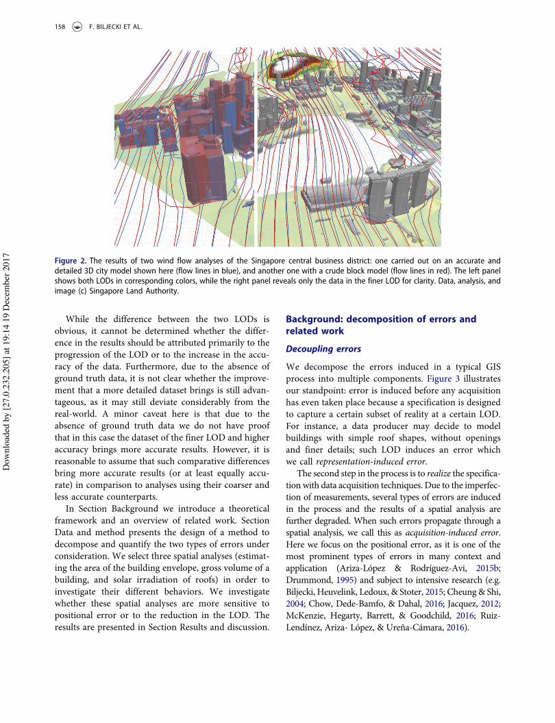
In this paper we focus on the most prominent LODcategorization, the one found in the OGC CityGMLstandard (Gröger & Plümer, 2012). The standarddefines LODs that progress in geometric detail andsemantic information: LOD1 is a block model, LOD2is a generalized model containing basic roof shapes,and LOD3 is an architecturally detailed model contain-ing openings and facade detail (Kolbe, Gröger, &Plümer, 2005).

These LODs roughly reflect the different outcomesof different acquisition techniques (Biljecki, Ledoux, &Stoter, 2016b). For instance, LOD1 is usually produced

by extruding footprints (Ledoux & Meijers, 2011),LOD2 can be acquired automatically from lidar data(Kada & McKinley, 2009), while LOD3 usually involvessubstantial manual work or is obtained after conver-sion from architectural sources (Donkers, Ledoux,Zhao, & Stoter, 2016). Examples of buildings modeledin these LODs will be exhibited in the next sections(Figures 4 and 5).

LOD3 marks the boundary of 3D GIS, as data offiner detail are considered to belong to the BuildingInformation Modeling arena. Moreover, LOD3 modelsare rarely used in spatial analyses and we are not awareof any LOD3 model produced on a large spatial scaledue to excessive costs of acquisition. Hence LOD3 is agood choice as ground truth reference data.

Selection of the spatial analyses

3D city models may be used for a variety of purposes,for instance, estimating the noise pollution at a location(Stoter, de Kluijver, & Kurakula, 2008), assessing visi-bility (Koltsova, Tunҫer, & Schmitt, 2013), and analyz-ing thermal comfort (Nichol & Wong, 2005). However,not all of the outcomes of these analyses result in aquantifiable result, which is a prerequisite for errorpropagation analyses as it provides a measure to

Figure 4. Two datasets of different LODs overlaid on an orthophoto (LOD1 – blue and LOD2 – yellow) of the same area but ofdifferent accuracy. The models are produced in separate campaigns, resulting in different positional accuracies and varyingcompleteness. Data (c) Swiss Federal Office of Topography.

162 F. BILJECKI ET AL.

Dow

nloa

ded

by [2

7.0.

232.

205]

at 1

9:14

19

Dec

embe

r 201

7

compare results. Several spatial analyses appear toderive ambiguous results, notwithstanding the chal-lenges of how to quantify them. For instance, 3D citymodels may be used for different kinds of visibilityanalyses, and therefore quantified in different ways:binary (a point in space is visible or not), distance(range) of visibility, the area or volume visible from apoint, number of buildings that have visual access to a

feature, and population that has visual access to a point(Cervilla, Tabik, Vías, Mérida, & Romero, 2016; Grassi& Klein, 2016; Wrózyński, Sojka, & Pyszny, 2016; Yuet al., 2016). Each one has different error propagationbehavior (Biljecki et al., 2017).

The error propagation task is further impeded bythe fact that capabilities of existing software are limited.In analyses such as this several building models are

Figure 5. Illustration of a subset of the experiments and results of one simulation on a sample of one 3D building model disturbedaccording to two different levels of accuracy (σx;y;z ¼ 0:2 and 0.5 m). The results from the three considered spatial analyses arelisted in the figure, and two types of errors are given for each case: the acquisition-induced error, and the combined error (inparentheses). This particular case is interesting because in the first two spatial analyses the LOD1 model inherently results in lessinaccurate results than the LOD2 model.

CARTOGRAPHY AND GEOGRAPHIC INFORMATION SCIENCE 163

Dow

nloa

ded

by [2

7.0.

232.

205]

at 1

9:14

19

Dec

embe

r 201

7

disturbed in hundreds of simulations, resulting in alarge abundance of datasets that have to be analyzed.Thus the capability to automatically and repeatedlyload the data and analyze the results is essential, sostudies such as this one entail the creation of customsoftware. Moreover, the large number of model runsentails an increased computational cost, which can besubstantial in some spatial analyses. For example, esti-mating the wind flow (as in Figure 2) may take a fewhours of computational time. Since Monte Carlo simu-lations involve repeated disturbances of data and re-running spatial analyses for hundreds if not thousandsof simulations, this can result in substantial simulationtime. Hence, it is important to select spatial analysesthat are feasible for Monte Carlo simulations.

We select the following three spatial analyses that wehave found to be appropriate for our research:

(1) Area of the building envelope. 3D city models aresuitable to calculate the area of the exposedbuilding shell. This information is useful inplanning energy-efficient retrofitting, estimatingindoor thermal comfort and energy consump-tion, analyzing the urban heat island effect, andfurther similar applications (Chwieduk, 2009;Deakin, Campbell, Reid, & Orsinger, 2014;Eicker, Nouvel, Duminil, & Coors, 2014;Maragkogiannis, Kolokotsa, Maravelakis, &Konstantaras, 2014; Nouvel, Schulte, Eicker,Pietruschka, & Coors, 2013; Perez, Kämpf, &Scartezzini, 2013; Previtali et al., 2014; van derHoeven & Wandl, 2015).

(2) Gross volume of a building. Estimation of thevolume of buildings is useful in various analyses,such as urban planning (Ahmed & Sekar, 2015),estimating the stock of materials in the buildingsector (Schebek et al., 2016), waste management(Mastrucci, Marvuglia, Popovici, Leopold, &Benetto, 2016), population estimation (Lwin &Murayama, 2009), quantifying developmentdensities (Meinel, Hecht, & Herold, 2009),energy estimation (Eicker et al., 2014; Nouvelet al., 2013), and predicting thermal comfort(Chwieduk, 2009; Perez et al., 2013).

(3) Solar irradiation of rooftops. Estimating theinsolation (solar exposure) of buildings is oneof the most prominent spatial analyses using 3Dcity models. The solar irradiation of rooftops iscalculated based on the orientation and inclina-tion of roofs, among other factors, whichinvolve spatial operations that are all prone toerrors. This application has wide applicability,for example, assessing the suitability of installing

solar panels (Szabó et al., 2016), preventingoverheating (Nichol & Wong, 2005), and pre-dicting house prices (Helbich, Jochem, Mücke,& Höfle, 2013). Typically the annual exposure tosun is estimated and quantified in kWh/m2

(Nault, Peronato, Rey, & Andersen, 2015). Wetake into account solar irradiation because it isan interesting use case, where the coarsest LODconsidered performs poorly because it only hasflat roofs, hence it is subject to large systematicerror. Due to computationally quite intensiveestimations we do not take shadowing intoaccount. However, the work of Biljecki et al.(2017) demonstrates that the LOD does nothave a significant influence on shadowestimation.

A particularity of our spatial analyses is that they areprone to positional errors that affect deformable objects(whose relative position can vary under uncertainty –for example, the width of the modeled building may besmaller than it is in reality). However, the analysesconsidered here is not affected by errors related topositional error in rigid objects (e.g. displacement of abuilding by 20 m due to processing errors does notalter its volume). For more on this topic the reader isreferred to Heuvelink, Brown, and van Loon (2007).

Procedural generation of the data

While it is reasonable to assume that using real-worlddata in the analyses is the best option, it is important tobe aware that real-world data are also burdened byacquisition errors. As a result, there is a risk of varyinglevels of quality and inconsistencies in the realizationof the specification. For instance, the LOD may not beconsistent across the dataset. In addition, real-worlddata have several other shortcomings making theiruse implausible. First, real-world 3D datasets are hardto perturb due to complex geometries, and they usuallycontain topological errors, not only preventing spatialanalyses but also making the simulations more difficultand prone to inconsistencies. Second, multi-LOD data-sets are rare (data producers usually produce data inone representation), and when they are available, theyare usually sourced from a different lineage; such inte-gration may induce additional errors or other types oferrors (and is therefore not comparable) (Figure 4).Third, an alternative to producing data in multipleLODs would be to take a fine LOD and obtain coarsercounterparts with generalization. However, data mod-eled in a fine LOD are seldom available, and whenavailable these are usually restricted to a small area,

164 F. BILJECKI ET AL.

Dow

nloa

ded

by [2

7.0.

232.

205]

at 1

9:14

19

Dec

embe

r 201

7

insufficiently large and diverse for experiments.Moreover, while research in 3D generalization is plen-tiful (Xie & Feng, 2016), there is no implementation weare aware of. The absence of data in fine LODs wouldmake experiments less interesting and would result inlack of a reference to gauge the results.

All of the above shortcomings can be solved by theuse of procedurally generated data as procedural mod-eling offers a sterile and controllable environment sui-ted for this problem. Procedural modeling involvesgenerating geographical data based on a set of custo-mized rules to represent a specific setting (Müller,Wonka, Haegler, Ulmer, & van Gool, 2006). Theirimportance in GIS is growing (Tsiliakou,Labropoulos, & Dimopoulou, 2014), for instance, toenhance existing data (Müller Arisona, Zhong,Huang, & Qin, 2013). In general, synthetic data havealready been in use in GIS when experimenting witherror and spatial analyses (Besuievsky et al., 2014;Burnicki, Brown, & Goovaerts, 2007; Erdélyi et al.,2014), and were proven powerful in testing diverseconfigurations.

An advantage of procedural models is that they can begenerated in a straightforward manner and for a largearea, and such an approach minimizes inconsistencies.Furthermore, the nature of procedural modeling war-rants that the models are produced according to a strictspecification which introduces no additional errors.

In this paper, we use a procedural modeling enginedeveloped by Biljecki, Ledoux, and Stoter (2016a),which generates 3D diverse building models, and cangenerate a fine representation in LOD3, which we useas reference data. The engine generates a diverse con-figuration of buildings (from small sheds to tall build-ings), warranting a variation of the input dataset.

Perturbation and grades of accuracy

3D city models may be derived with differentapproaches involving diverse technologies, each withdifferent capabilities when it comes to the accuracy.Hence, it is important to investigate different magni-tudes of positional error (standard deviation σ).

In our approach, we simulate positional error bydegrading the geometry of a 3D city model with valuessampled from a normal probability distribution func-tion with standard deviation σ, which is in line withrelated work (Ben-Haim, Dalyot, & Doytsher, 2015;Brown & Heuvelink, 2007; Xue et al., 2016). The ver-tices of the 3D model are disturbed while retainingright angles to mimic common acquisition approachesof the data, such as photogrammetric mapping.

Our approach assumes that there is no correlation inthe errors in different dimensions.We follow the assump-tion of uncorrelated errors in coordinates. 3D city modelsare often acquired in different acquisition campaigns (e.g.footprints are acquired with a geodetic survey, while theelevation of the building is acquired with airborne laserscanning). However, we acknowledge that correlatederrors may influence the outcome of the analysis, asdemonstrated by Navratil and Achatschitz (2004).

With the exception of satellite platforms (Duan &Lafarge, 2016; Toth & Jóźków, 2016), researchers reg-ularly report submeter accuracy of 3D acquisition tech-niques (Jarząbek-Rychard & Borkowski, 2016;Kabolizade, Ebadi, & Mohammadzadeh, 2012;Mårtensson & Reshetyuk, 2016; Rottensteiner et al.,2014; Wang, Kutterer, & Fang, 2016). Hence, we con-sider positional accuracy in the range of 0–1 m in10 cm increments resulting in 11 error classes. Takinginto consideration multiple accuracy classes also helpsin understanding the impact that increasing the errorof the input has on the error of the output.

Because of the integration of data from different sourcesand the nature of acquisition methods, another point thatwe consider is the varying level of accuracy in the planarand vertical coordinates (σx;y!σz). While this is an inher-ent property of 3D acquisition techniques such as laserscanning (Gil de la Vega, Ariza-López, & Mozas-Calvache, 2016; Goulden et al., 2016; McClune, Mills,Miller, & Holland, 2016), the varying accuracies are espe-cially emphasized in cases such where building footprintsand heights were derived in separate measurements, forexample, footprints from ground measurements andheights guessed from the number of storeys orwith anothermethod of incomparable accuracy. In such cases the differ-ence between planar and vertical accuracies may be sub-stantial, so for each of σx;y and σz we combine 11 classesresulting in 121 independent accuracy classes. LOD3 is anexception as the perturbations were carried out up to σ ¼0:3 m, as in reality the error is not larger than that.

Implementation

We generated a dataset of 100 3D building models inCityGML and perturbed these in 1000 iterations usingMonte Carlo simulation, according to 121 accuracyclasses resulting in 12.1 million cases to be analyzed.The methodology is described in Biljecki et al. (2015).

An example of a part of the simulations is shown inFigure 5. The simulations and the spatial analyses tookseveral weeks. During the simulations, there were someoccasions with excessive acquisition-induced errors,causing the realization of data containing topological

CARTOGRAPHY AND GEOGRAPHIC INFORMATION SCIENCE 165

Dow

nloa

ded

by [2

7.0.

232.

205]

at 1

9:14

19

Dec

embe

r 201

7

errors. Our implementation includes a built-in validatoraccording to international standards in GIS (Ledoux,2013), therefore simulations that had topological errorswere discarded to avoid the introduction of inconsisten-cies other than positional errors.

Results and discussion

Due to the large number of results we specifically focuson the most important findings. We present the resultsgraphically in plots and tables, and describe them inthe text. Furthermore, in order for a direct comparisonof results between different spatial analyses, we presentthe errors in percentages of the true value.

Representation-induced errors

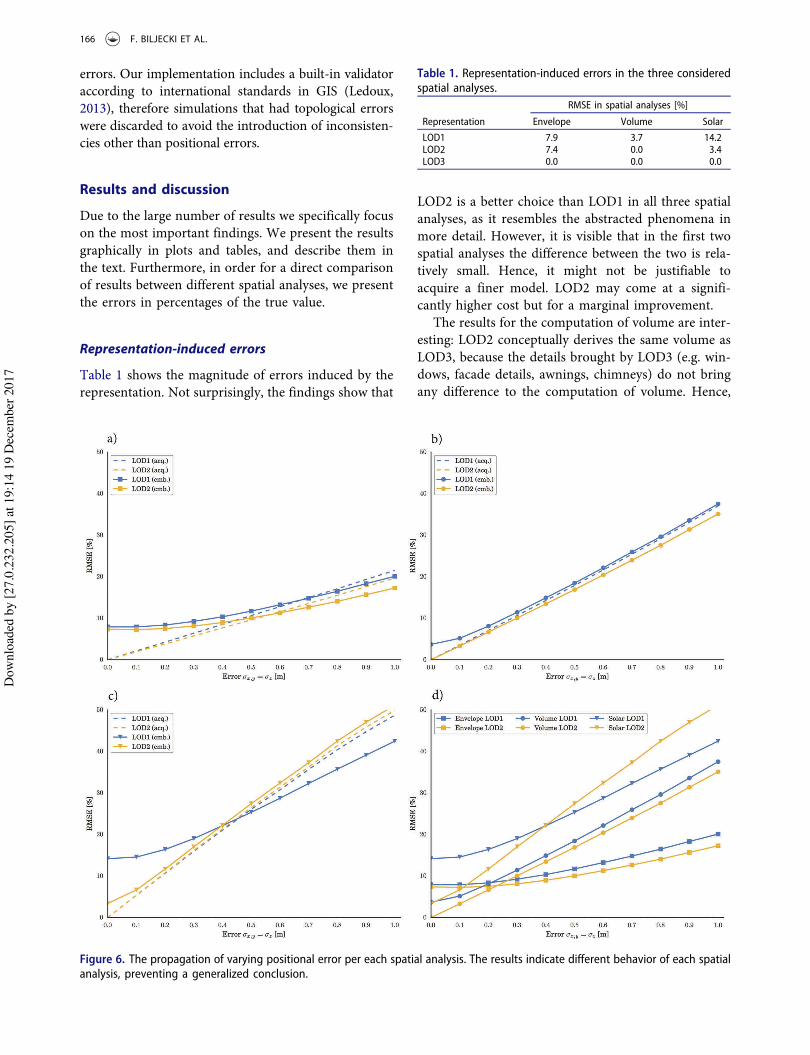
Table 1 shows the magnitude of errors induced by therepresentation. Not surprisingly, the findings show that

LOD2 is a better choice than LOD1 in all three spatialanalyses, as it resembles the abstracted phenomena inmore detail. However, it is visible that in the first twospatial analyses the difference between the two is rela-tively small. Hence, it might not be justifiable toacquire a finer model. LOD2 may come at a signifi-cantly higher cost but for a marginal improvement.

The results for the computation of volume are inter-esting: LOD2 conceptually derives the same volume asLOD3, because the details brought by LOD3 (e.g. win-dows, facade details, awnings, chimneys) do not bringany difference to the computation of volume. Hence,

Table 1. Representation-induced errors in the three consideredspatial analyses.

RMSE in spatial analyses [%]

Representation Envelope Volume Solar

LOD1 7.9 3.7 14.2LOD2 7.4 0.0 3.4LOD3 0.0 0.0 0.0

Figure 6. The propagation of varying positional error per each spatial analysis. The results indicate different behavior of each spatialanalysis, preventing a generalized conclusion.

166 F. BILJECKI ET AL.

Dow

nloa

ded

by [2

7.0.

232.

205]

at 1

9:14

19

Dec

embe

r 201

7

ignoring acquisition errors at this point, it appears thatLOD3 does not bring any benefit over LOD2 when itcomes to the computation of gross volume.

Acquisition-induced errors

The results shown in Section Representation-inducederrors indicate the magnitude of error if the modelswere (theoretically) acquired without acquisition errors.This section first considers the effect of positional errorsin isolation. These effects are visualized in the dashedlines of Figure 6, for each spatial analysis separately.

The results indicate that the error propagates linearlyin all three analyses, but that it has a different impact onthe final result. For instance, the error induced by acqui-sition scenario σx;y ¼ 0:4 m/σz ¼ 0:2 m for the threeanalyses is 6.6%, 12.6%, and 20.8%, respectively.

The propagation of positional error is similarbetween LODs in all three spatial analyses. However,notice that in the first experiment the error for LOD1(dashed blue line) is larger than that of LOD2 (dashedyellow line), which is not the case for the third spatialanalysis, while in the second experiment they coincide.This result suggests that positional error affects differ-ent LODs in different spatial analyses in different ways.

Two errors in combination

Figure 6 shows the combination of the two errors as solidlines. In addition, the plot in the bottom right shows thecombined errors jointly for the three spatial analyses forcomparison. The representation-induced error is alsoprovided in the plots: this is the case where σ ¼ 0.

The results suggest that the combined effect of the twoerror sources is not additive but is much more complexthan that. The reason has to be studied in furtherresearch. The results also indicate that LOD2 is in mostcases better than LOD1 by a thin margin, which means

that despite the added positional error, the finer LOD2still offers a slight benefit over the coarser LOD1.

However, the propagation of error in the third experi-ment gives unexpected results. LOD1 has an unfavorablestarting point (the representation induces gross errorsowing to flat rooftops), but eventually at σ ¼ 0:5 m itsurpasses the accuracy of the analysis with LOD2, probablyowing to the more complex geometry of LOD2. A secondunexpected result occurs in the first experiment (envelopearea): the acquisition error (dashed line) is larger than thecombined error (solid line), for both LOD1 and LOD2.These results indicate the presence of a systematic error.

Recall the dilemma discussed in the introduction inregard to using a dataset of a finer LOD but of lesseraccuracy in contrast to the inverse situation. In ourexperiments an LOD1 acquired with σ ¼ 0:2 m is amuch better choice than the finer LOD2 acquired withpoorer accuracy (σ ¼ 0:5 m); see Table 2 for compar-ison of all three considered spatial analyses.

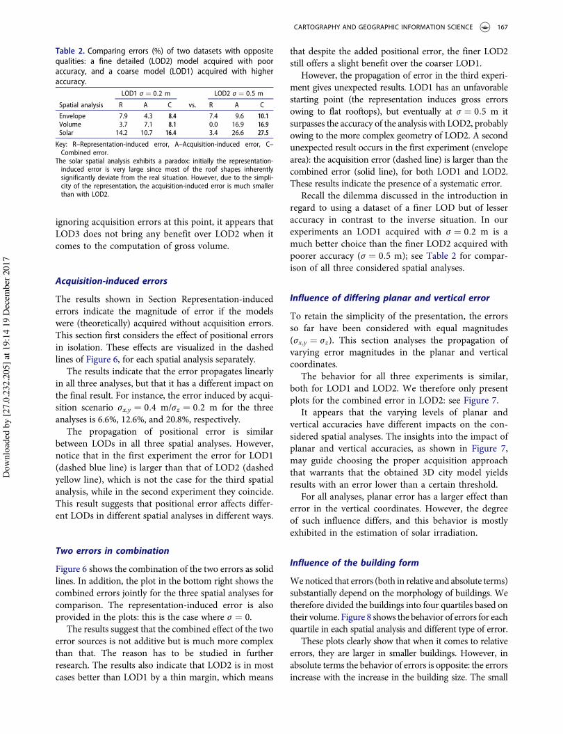
Influence of differing planar and vertical error

To retain the simplicity of the presentation, the errorsso far have been considered with equal magnitudes(σx;y ¼ σz). This section analyses the propagation ofvarying error magnitudes in the planar and verticalcoordinates.

The behavior for all three experiments is similar,both for LOD1 and LOD2. We therefore only presentplots for the combined error in LOD2: see Figure 7.

It appears that the varying levels of planar andvertical accuracies have different impacts on the con-sidered spatial analyses. The insights into the impact ofplanar and vertical accuracies, as shown in Figure 7,may guide choosing the proper acquisition approachthat warrants that the obtained 3D city model yieldsresults with an error lower than a certain threshold.

For all analyses, planar error has a larger effect thanerror in the vertical coordinates. However, the degreeof such influence differs, and this behavior is mostlyexhibited in the estimation of solar irradiation.

Influence of the building form

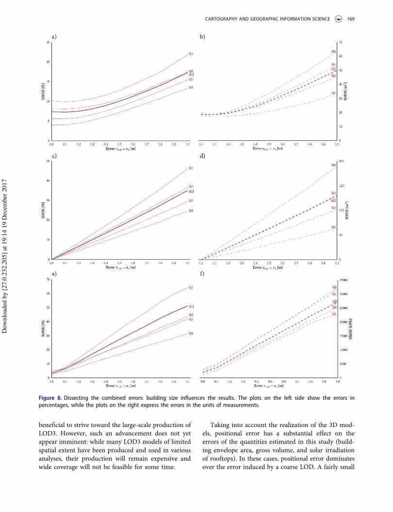
Wenoticed that errors (both in relative and absolute terms)substantially depend on the morphology of buildings. Wetherefore divided the buildings into four quartiles based ontheir volume. Figure 8 shows the behavior of errors for eachquartile in each spatial analysis and different type of error.

These plots clearly show that when it comes to relativeerrors, they are larger in smaller buildings. However, inabsolute terms the behavior of errors is opposite: the errorsincrease with the increase in the building size. The small

Table 2. Comparing errors (%) of two datasets with oppositequalities: a fine detailed (LOD2) model acquired with pooraccuracy, and a coarse model (LOD1) acquired with higheraccuracy.

LOD1 σ ¼ 0:2 m LOD2 σ ¼ 0:5 m

Spatial analysis R A C vs. R A C

Envelope 7.9 4.3 8.4 7.4 9.6 10.1Volume 3.7 7.1 8.1 0.0 16.9 16.9Solar 14.2 10.7 16.4 3.4 26.6 27.5

Key: R–Representation-induced error, A–Acquisition-induced error, C–Combined error.

The solar spatial analysis exhibits a paradox: initially the representation-induced error is very large since most of the roof shapes inherentlysignificantly deviate from the real situation. However, due to the simpli-city of the representation, the acquisition-induced error is much smallerthan with LOD2.

CARTOGRAPHY AND GEOGRAPHIC INFORMATION SCIENCE 167

Dow

nloa

ded

by [2

7.0.

232.

205]

at 1

9:14

19

Dec

embe

r 201

7

exception in the third experiment (right plot in the bottomrow; showing different order for Q3 and Q4) is caused bythe varying degrees of insolation of roof surfaces. That is,rooftops with smaller areas may have a higher amount ofsolar irradiation than larger rooftops, so that rooftops ofsmaller buildings may have a larger absolute error in solarirradiation than rooftops of larger buildings.

These results imply that the outcome of analyses such asthese also depend on the base dataset that is used, primarilybecause these are driven by the morphology of the build-ings. In 2D this topic has been investigated by Berk andFerlan (2016), pointing out that the size and the shape of aparcel may characterize the propagation of error whencalculating its area.

General discussion and key findings

A major finding of this paper is that taking care of theaccuracy of the data is more important than striving to

produce data of a finer LOD, at least in the spatialanalyses that we considered.

LOD1 and LOD2 are significantly different models –they are acquired with different approaches with thelatter being more complex to produce. Despite suchdistinction, when used in the first two spatial analyses(envelope area and gross volume) the difference in theperformance of LOD1 and LOD2 is so small that itappears that in many cases it is not worth acquiring anLOD2. For instance, when an LOD1 is used in theestimation of envelope area the RMSE is 7.9%, andLOD2 shaves off the error to 7.4%, which is practicallynegligible. In such cases it may be more favorable touse the coarser LOD1–they are simpler to acquire, theyhave a smaller storage footprint, and they are faster toprocess. Hence the increased costs for obtaining thefiner LOD2 may not always be justified.

The leap between LOD2 and LOD3 is much largerthan between LOD1 and LOD2. Hence it would be

Figure 7. Contour plots showing the influence of variable accuracy levels onto the error of the three spatial analyses for LOD2. Notethat the color ranges vary among plots. The bottom right plot exposes the differences in error propagation by showing thesensitivity of the spatial analyses at a certain threshold (value of 10% RMSE).

168 F. BILJECKI ET AL.

Dow

nloa

ded

by [2

7.0.

232.

205]

at 1

9:14

19

Dec

embe

r 201

7

beneficial to strive toward the large-scale production ofLOD3. However, such an advancement does not yetappear imminent: while many LOD3 models of limitedspatial extent have been produced and used in variousanalyses, their production will remain expensive andwide coverage will not be feasible for some time.

Taking into account the realization of the 3D mod-els, positional error has a substantial effect on theerrors of the quantities estimated in this study (build-ing envelope area, gross volume, and solar irradiationof rooftops). In these cases, positional error dominatesover the error induced by a coarse LOD. A fairly small

Figure 8. Dissecting the combined errors: building size influences the results. The plots on the left side show the errors inpercentages, while the plots on the right express the errors in the units of measurements.

CARTOGRAPHY AND GEOGRAPHIC INFORMATION SCIENCE 169

Dow

nloa

ded

by [2

7.0.

232.

205]

at 1

9:14

19

Dec

embe

r 201

7

error of 0.2 m outweighs the benefit of a fine LOD, andour results indicate that in two of the three consideredspatial analyses, an LOD1 acquired with σ ¼ 0:2 m is amuch better choice than the finer LOD2 acquired withpoorer accuracy (σ ¼ 0:5 m). However, this is not thecase for the solar irradiation of rooftops use case, inwhich LOD1 cannot be used due to its systematicshortcoming of having flat roofs. A paradox in thisspatial analysis is that at poorer accuracies the errorby LOD1 is smaller, due to the high sensitivity of solarirradiation estimation to positional errors.

The combined error cannot be simply decoupledinto representation- and acquisition-induced errorbecause they do not sum up. This is also obviousfrom the errors given in Figure 5, see for instance thecase of LOD1 disturbed with σ ¼ 0:5 m. Such resultindicates that there are interactions between the errors,as they are not additive.

These experiments provide insight into designingspecifications of 3D city models while taking intoaccount the intended spatial analyses; the increase ofdetail does conceptually bring some benefit, but inpractice, when models are realized (and hence affectedby the imperfection of measurement) the benefit iscountervailed by acquisition errors. As a consequence,the representation benefit between LOD1 and LOD2becomes negligible.

The results also show that each spatial analysis hasdifferent behavior. Hence, it is important to considereach spatial analysis separately in experiments. As thework also suggests that spatial analyses have a substan-tially different behavior when compared to each other,data suitable for one spatial analysis may be of littlevalue for another.

Real-world data offer little room for manoeuvre inexperiments such as ours, hence we suggest researchersin related work resorting to procedurally generatedmodels as their benefit in such analyses is underesti-mated and unparalleled. By using a proceduralapproach we were able to obtain models that are bur-dened only with the errors we want (e.g. we did nothave to worry that other errors such as completenesscould have compromised our analysis), and by indu-cing specific errors in a simulation we could isolate theinfluence of different errors. On the other hand, itshould be noted that synthetic data might not alwaysproperly represent real-world data.

A limitation of our study is that we do not addressthe inability of software to take advantage of finerLODs. For example, in theory there could be a sub-stantial difference between using LOD1 and LOD2 forestimating noise pollution (e.g. sloped roofs henceforthavailable in LOD2 may bounce the noise in a different

way resulting in substantially different predictions, seeVan Renterghem and Botteldooren (2010) whichdemonstrates that roof shapes are an important factorto consider in noise pollution estimations). However,the software may simply not be capable of takingadvantage of the more detailed geometry of the roof-tops (e.g. it considers only the bounding box of abuilding), and will give the same results as for LOD1.

Looking into this matter is certainly our priorityfor future work, and for this, we plan to follow theapproach of Ruiz Arias et al. (2009). In their analysisinvolving rasters of multiple resolutions, they com-pare the results from multiple software packages andconclude that some software solutions lead to largererror propagation. In our analysis we have dealt withvolume and area computation, which should notdiffer between different software packages (when weprogrammed the two we compared the results fromanother software for validation). However, this isprobably not the case for the solar irradiation usecase, especially because due to computationallyintensive calculations it was not possible to takeinto account shadowing effects. In the context ofthis paper, the absence of shadowing is an exampleof a factor in the analysis-induced error.

Another aspect that we did not address, is that it isnot always possible to separate the LOD and positionalerrors. Sometimes they are fused, for example, a com-plex building footprint may be simplified as a rectan-gle, and at the same time its geometry may be displaceddue to generalization rules. That is, because in coarserscales such a rectangle would encompass the building(e.g. a bounding box) and the vertices would not cor-respond across multiple LODs (Arroyo Ohori, Ledoux,Biljecki, & Stoter, 2015). In 3D GIS, LOD1 and LOD2are usually realized using the same footprints (Biljeckiet al., 2016b), hence this does not affect much of ourwork and while we do not contend that we have asolution here, it is certainly important to acknowledgethe occasionally blurry distinction between representa-tion and acquisition errors.

Finally, to maintain a reasonable level of simplicity,this study did not take into account potential systema-tic errors such as projection errors (Chrisman, 2016;Girres, 2011), which may – together with the errorscaused by ignoring terrain elevation – affect the build-ing footprint dimensions (Berk & Ferlan, 2016).

Conclusions

LOD and positional accuracy are arguably some of themain ingredients in the metadata of most GIS datasets.In this paper we performed a combined (multiple) error

170 F. BILJECKI ET AL.

Dow

nloa

ded

by [2

7.0.

232.

205]

at 1

9:14

19

Dec

embe

r 201

7

propagation analysis that demonstrates how much erroris induced on top of error caused by using differentLODs. Our main contribution in the subject of errorpropagation is that we take into account simultaneouslymultiple types of errors, and we consider multiple spatialanalyses. While errors may be induced at many differentpoints in a typical GIS process (Gahegan & Ehlers, 2000;Lunetta et al., 1991), we deem that acquisition- andrepresentation-induced errors are the most prominentones, hence we focused on them.

The main conclusions of this paper are: (i) thepositional error is in many cases significantly moredominant than representation error; (ii) as a result ofthis, in a lot of instances there is no need to go for ahigh representation level (LOD3) because the addedvalue will vanish due to acquisition error; (iii) the twoconsidered errors are not additive; (iv) error propaga-tion is case specific, hence there is no general conclu-sion that can be drawn for all spatial analyses; and (v)when disturbed with larger positional errors a lowerrepresentation may give better results in a spatial ana-lysis than a higher representation disturbed with theerror of the same magnitude.

This paper also suggests that LOD in 3D GIS andscale in 2D GIS are related but different concepts. Scalein 2D is mainly associated with accuracy and precision,with less detail on small-scale maps, while for 3D thatrelation does not always hold. In 3D data of coarsedetail at a high precision/accuracy level is common,regardless of the spatial scale.

Plans for future work are to investigate the behaviorof the propagated error in other spatial analyses, and toinvestigate the behavior of correlated errors as thesemay significantly impact the error propagation(Navratil & Achatschitz, 2004). Correlations betweenpositional errors can be incorporated in a probabilisticmodel but will require stationarity assumptions to limitthe number of model parameters (Heuvelink et al.,2007). Furthermore, we intend to consider other typesof acquisition error common in geoinformation, suchas completeness, which next to positional accuracy iscommonly cited as a principal acquisition-inducederror (Ariza-López & Rodríguez-Avi, 2015a; Demir,2015). Finally, a continuation of the work would beto consider the bigger picture of errors and analyzetheir consequences by associating them to a meaningfulapplication. For example, the impact of a 10% error inthe estimation of volume depends on the intended useof the derived information. If the volume was used todetermine property tax, an error of 10% would not beacceptable. However, if it was used to estimate thevolumetric building stock of a complete neighborhoodfor heating demand estimation or for population

estimation, on a large scale such error might be lesssevere as the errors would probably cancel out inthe sum.

Acknowledgments

We thank the three anonymous reviewers for providinginsightful comments which have improved the paper. Weappreciate the sample data and visuals provided by theSingapore Land Authority, Swiss Federal Office ofTopography, and OpenStreetMap contributors. The licensefor FME was kindly provided by Safe Software Inc. Wegratefully acknowledge the discussions with Niko Lukač(University of Maribor), Giuseppe Peronato (Swiss FederalInstitute of Technology in Lausanne), Romain Nouvel (HFTStuttgart), and Anna Labetski (TU Delft).

Disclosure statement

No potential conflict of interest was reported by the authors.

Funding

This research is supported by the Dutch TechnologyFoundation STW, which is part of the NetherlandsOrganisation for Scientific Research (NWO), and which ispartly funded by the Ministry of Economic Affairs (projectcode: 11300).

ORCID

Filip Biljecki http://orcid.org/0000-0002-6229-7749Gerard B.M. Heuvelink http://orcid.org/0000-0003-0959-9358Hugo Ledoux http://orcid.org/0000-0002-1251-8654Jantien Stoter http://orcid.org/0000-0002-1393-7279

References

Ahmed, F. C., & Sekar, S. P. (2015). Using three-dimensionalvolumetric analysis in everyday urban planning processes.Applied Spatial Analysis and Policy, 8(4), 393–408.doi:10.1007/s12061-014-9122-2

Ariza-López, F. J., & Rodríguez-Avi, J. (2015a). Estimatingthe count of completeness errors in geographic data setsby means of a generalized Waring regression model.International Journal of Geographical Information Science,29(8), 1394–1418. doi:10.1080/13658816.2015.1010536

Ariza-López, F. J., & Rodríguez-Avi, J. (2015b). Using inter-national standards to control the positional quality ofspatial data. Photogrammetric Engineering and RemoteSensing, 81(8), 657–668. doi:10.14358/PERS.81.8.657

Arroyo Ohori, K., Ledoux, H., Biljecki, F., & Stoter, J. (2015).Modeling a 3D city model and its levels of detail as a true4D model. ISPRS International Journal of Geo-Information, 4(3), 1055–1075. doi:10.3390/ijgi4031055

Beekhuizen, J., Heuvelink, G. B. M., Huss, A., Bürgi, A.,Kromhout, H., & Vermeulen, R. (2014). Impact of input

CARTOGRAPHY AND GEOGRAPHIC INFORMATION SCIENCE 171

Dow

nloa

ded

by [2

7.0.

232.

205]

at 1

9:14

19

Dec

embe

r 201

7

data uncertainty on environmental exposure assessmentmodels: A case study for electromagnetic field modellingfrom mobile phone base stations. Environmental Research,135, 148–155. doi:10.1016/j.envres.2014.05.038

Ben-Haim, G., Dalyot, S., & Doytsher, Y. (2015). Local absolutevertical accuracy computation of wide-coverage digital ter-rain models. In F. Harvey and Y. Leung (Eds.), Advances inspatial data handling and analysis (pp. 209–225). Cham,Switzerland: Springer International. doi:10.1007/978-3-319-19950-4_13

Berk, S., & Ferlan, M. (2016). Accurate area determination inthe cadaster: Case study of Slovenia. Cartography andGeographic Information Science. Advance online publica-tion. doi:10.1080/15230406.2016.1217789

Besuievsky, G., Barroso, S., Beckers, B., & Patow, G. (2014).A configurable LoD for procedural urban models intendedfor daylight simulation. In G. Besuievsky & V. Tourre(Eds.), Eurographics workshop on urban data modellingand visualisation (pp. 19–24). Aire-la-Ville, Switzerland:Eurographics Association. doi:10.2312/udmv.20141073

Biljecki, F., Heuvelink, G. B. M., Ledoux, H., & Stoter, J.(2015). Propagation of positional error in 3D GIS:Estimation of the solar irradiation of building roofs.International Journal of Geographical InformationSciences, 29(12), 2269–2294. doi:10.1080/13658816.2015.1073292

Biljecki, F., Ledoux, H., & Stoter, J. (2016a). Generation of multi-LOD 3D city models in CityGML with the procedural model-ling engine Random3Dcity. ISPRS Annals PhotogrammRemote Sensing Spatial Information Sciences IV-4/W1, 51–59. doi:10.5194/isprs-annals-IV-4-W1-51-2016

Biljecki, F., Ledoux, H., & Stoter, J. (2016b). An improvedLOD specification for 3D building models. Computers,Environment and Urban Systems, 59, 25–37. doi:10.1016/j.compenvurbsys.2016.04.005

Biljecki, F., Ledoux, H., & Stoter, J. (2017). Does a finer levelof detail of a 3D city model bring an improvement forestimating shadows? In A. Abdul-Rahman (Ed.), Advancesin 3D geoinformation (pp. 31–47). Cham, Switzerland:Springer International. doi:10.1007/978-3-319-25691-7_2

Biljecki, F., Ledoux, H., Stoter, J., & Vosselman, G. (2016).The variants of an LOD of a 3D building model and theirinfluence on spatial analyses. ISPRS Annals of thePhotogrammetry, Remote Sensing and Spatial InformationSciences, 116, 42–54. doi:10.1016/j.isprsjprs.2016.03.003

Biljecki, F., Ledoux, H., Stoter, J., & Zhao, J. (2014).Formalisation of the level of detail in 3D city modelling.Computers, Environment and Urban Systems, 48, 1–15.doi:10.1016/j.compenvurbsys.2014.05.004

Billger, M., Thuvander, L., & Wästberg, B. S. (2016). Insearch of visualization challenges: The development andimplementation of visualization tools for supporting dia-logue in urban planning processes. Environment andPlanning B: Planning and Design. Advance online publica-tion. doi:10.1177/0265813516657341

Boeters, R., Arroyo Ohori, K., Biljecki, F., & Zlatanova, S.(2015). Automatically enhancing CityGML LOD2 modelswith a corresponding indoor geometry. InternationalJournal of Geographical Information Science, 29(12),2248–2268. doi:10.1080/13658816.2015.1072201

Booij, M. J. (2005). Impact of climate change on river flood-ing assessed with differ- ent spatial model resolutions.

Journal of Hydrology, 303(1–4), 176–198. doi:10.1016/j.jhydrol.2004.07.013

Brasebin, M., Perret, J., Mustière, S., & Weber, C. (2012).Measuring the impact of 3D data geometric modeling onspatial analysis: Illustration with Skyview factor. In T.Leduc, G. Moreau, & R. Billen (Eds.), Usage, usability,and utility of 3D city models – European cost actiontu0801 (02001)1–16). Les Ulis, France: EDP Sciences.doi:10.1051/3u3d/201202001

Bremer, M., Mayr, A., Wichmann, V., Schmidtner, K., &Rutzinger, M. (2016). A new multi-scale 3D-GIS-approachfor the assessment and dissemination of solar income of digitalcity models. Computers, Environment and Urban Systems, 57,144–154. doi:10.1016/j.compenvurbsys.2016.02.007

Brown, J. D., & Heuvelink, G. B. M. (2007). The data uncer-tainty engine (DUE): A software tool for assessing and simu-lating uncertain environmental variables. Computers &Geosciences, 33(2), 172–190. doi:10.1016/j.cageo.2006.06.015

Bruse,M., Nouvel, R.,Wate, P., Kraut, V., &Coors, V. (2015). Anenergy-related cityGML ADE and its application for heatingdemand calculation. International Journal of 3-D InformationModeling, 4(3), 59–77. doi:10.4018/IJ3DIM.2015070104

Burnicki, A. C., Brown, D. G., & Goovaerts, P. (2007).Simulating error propagation in land-cover change analy-sis: The implications of temporal dependence. Computers,Environment and Urban Systems, 31(3), 282–302.doi:10.1016/j.compenvurbsys.2006.07.005

Burrough, P. A., & McDonnell, R. A. (1998). Errors andquality control. In P. A. Burrough, R. A. McDonnell,and C. D. Lloyd (Eds.), Principles of geographical infor-mation systems (pp. 220–240). Oxford: OxfordUniversity Press.

Camboim, S., Bravo, J., & Sluter, C. (2015). An investigationinto the completeness of, and the updates to, openstreet-map data in a heterogeneous area in Brazil. ISPRSInternational Journal of Geo-Information, 4(3), 1366–1388. doi:10.3390/ijgi4031366

Cervilla, A. R., Tabik, S., Vías, J., Mérida, M., & Romero, L.F. (2016). Total 3D-viewshed map: Quantifying the visiblevolume in digital elevation models. Transactions in GIS.Advance online publication. doi:10.1111/tgis.12216

Chaubey, I., Cotter, A. S., Costello, T. A., & Soerens, T. S.(2005). Effect of DEM data resolution on SWAT outputuncertainty. Hydrological Processes, 19(3), 621–628.doi:10.1002/hyp.5607

Cheung, C. K., & Shi, W. (2004). Estimation of the positionaluncertainty in line simplification in GIS. The CartographicJournal, 41(1), 37–45. doi:10.1179/000870404225019990

Chow, T. E., Dede-Bamfo, N., & Dahal, K. R. (2016).Geographic disparity of positional errors and matchingrate of residential addresses among geocoding solu-tions. Annals of GIS, 22(1), 29–42. doi:10.1080/19475683.2015.1085437

Chrisman, N. (1991). The error component in spatial data.In P. A. Longley, M. F. Goodchild, D. J. Maguire, & D.W. Rhind (Eds.), Geographical information systems:Principles and applications (pp. 165–174). Harlow, UK:Longmans.

Chrisman, N. R. (2016). Calculating on a round planet.International Journal of Geographical InformationScience. Advance online publication. doi:10.1080/13658816.2016.1215466

172 F. BILJECKI ET AL.

Dow

nloa

ded

by [2

7.0.

232.

205]

at 1

9:14

19

Dec

embe

r 201

7

Chwieduk, D. A. (2009). Recommendation on modelling ofsolar energy incident on a building envelope. RenewableEnergy, 34(3), 736–741. doi:10.1016/j.renene.2008.04.005

Couturier, S., Mas, J.-F., Cuevas, G., Benítez, J., Vega-Guzman, A., & Coria-Tapia, V. (2009). An accuracyindex with positional and thematic fuzzy bounds forland-use/land-cover maps. Photogrammetric Engineeringand Remote Sensing, 75(7), 789–805. doi:10.14358/PERS.75.7.789

Cromley, R. G., Lin, J., & Merwin, D. A. (2012).Evaluating representation and scale error in the max-imal covering location problem using GIS and intelli-gent areal interpolation. International Journal ofGeographical Information Science, 26(3), 495–517.doi:10.1080/13658816.2011.596840

de Bruin, S., Heuvelink, G. B. M., & Brown, J. D. (2008).Propagation of positional measurement errors to agricul-tural field boundaries and associated costs. Computers andElectronics in Agriculture, 63(2), 245–256. doi:10.1016/j.compag.2008.03.005

Deakin, M., Campbell, F., Reid, A., & Orsinger, J. (2014). Themass retrofitting of an energy efficient—Low carbon zone.London: Springer. doi:10.1007/978-1-4471-6621-4

Demir, N. (2015). Use of airborne laser scanning data andimage-based three-dimensional (3-D) edges for automatedplanar roof reconstruction. Lasers in Engineering, 32(3–4),173–205.

Deng, Y., & Cheng, J. C. P. (2015). Automatic transformationof different levels of detail in 3D GIS city models inCityGML. International Journal of 3-D InformationModeling, 4(3), 1–21. doi:10.4018/IJ3DIM.2015070101

Deng, Y., Cheng, J. C. P., & Anumba, C. (2016). Aframework for 3D traffic noise mapping using datafrom BIM and GIS integration. Structure andInfrastructure Engineering, 12(10), 1267–1280.doi:10.1080/15732479.2015.1110603

Donkers, S., Ledoux, H., Zhao, J., & Stoter, J. (2016).Automatic conversion of IFC datasets to geometricallyand semantically correct CityGML LOD3 buildings.Transactions in GIS, 20(4), 547–569. doi:10.1111/tgis.12162

Drummond, J. (1995). Positional accuracy. In S. C. Guptilland J. L. Morrison (Eds.), Elements of spatial data quality(pp. 31–58). Oxford: Elsevier. doi:10.1016/B978-0-08-042432-3.50010-0

Duan, L., & Lafarge, F. (2016). Towards large-scale cityreconstruction from satellites. In B. Leibe, J. Matas, N.Sebe, M. Welling (Eds.). Computer Vision - ECCV 2016(pp. 89–104). Cham, Switzerland: Springer International.doi:10.1007/978-3-319-46454-1_6

Eicker, U., Nouvel, R., Duminil, E., & Coors, V. (2014).Assessing passive and active solar energy resources incities using 3D city models. Energy Procedia, 57, 896–905. doi:10.1016/j.egypro.2014.10.299

Ellul, C., Adjrad, M., & Groves, P. (2016). The impact of 3Ddata quality on improving GNSS performance using citymodels initial simulations. ISPRS Annals of thePhotogrammetry, Remote Sensing and Spatial InformationSciences, IV-2-W1, 171–178. doi:10.5194/isprs-annals-IV-2-W1-171-2016

Ellul, C., & Altenbuchner, J. (2013). LOD 1 VS. LOD 2 –Preliminary investigations into differences in mobile

rendering performance. ISPRS Annals of thePhotogrammetry, Remote Sensing and Spatial InformationSciences, II-2/W1, 129–138. doi:10.5194/isprsannals-II-2-W1-129-2013

Erdélyi, R., Wang, Y., Guo, W., Hanna, E., & Colantuono, G.(2014). Three- dimensional SOlar RAdiation Model(SORAM) and its application to 3-D urban planning.Solar Energy, 101, 63–73. doi:10.1016/j.solener.2013.12.023

Fai, S., & Rafeiro, J. (2014). Establishing an appropriate level ofdetail (LoD) for a building information model (BIM) – WestBlock, Parliament Hill, Ottawa, Canada. ISPRS Annals of thePhotogrammetry, Remote Sensing and Spatial InformationSciences, II-5, 123–130. doi:10.5194/isprsannals-II-5-123-2014

Fan, H., Zipf, A., Fu, Q., & Neis, P. (2014). Quality assess-ment for building footprints data on OpenStreetMap.International Journal of Geographical Information Science,28(4), 700–719. doi:10.1080/13658816.2013.867495

Freitas, S., Cristóvão, A., Amaro e Silva, R., & Brito, M. C.(2016). Obstruction surveying methods for PV applicationin urban environments. In Proceedings of the 32ndEuropean photovoltaic solar energy conference and exhibi-tion (pp. 2759-2764). WIP: Munich. doi:10.4229/EUPVSEC20162016-6AV.5.18

Gahegan, M., & Ehlers, M. (2000). A framework for themodelling of uncertainty between remote sensing andgeographic information systems. ISPRS Journal ofPhotogrammery and Remote Sensing, 55(3), 176–188.doi:10.1016/S0924-2716(00)00018-6

Gil de la Vega, P., Ariza-López, F. J., & Mozas-Calvache, A.T. (2016). Models for positional accuracy assessment oflinear features: 2D and 3D cases. Survey Review, 48(350),347–360. doi:10.1080/00396265.2015.1113027

Girres, J.-F. (2011, October). A model to estimate length mea-surements uncertainty in vector databases. Paper presentedat the 7th International Symposium on Spatial Data Quality(ISSDQ’11), Coimbra, Portugal.

Goodchild, M. F., & Li, L. (2012). Assuring the quality ofvolunteered geographic information. Spatial Statistics, 1,110–120. doi:10.1016/j.spasta.2012.03.002

Goulden, T., Hopkinson, C., Jamieson, R., & Sterling, S. (2016).Sensitivity of DEM, slope, aspect and watershed attributes toLiDAR measurement uncertainty. Remote Sensing ofEnvironment, 179, 23–35. doi:10.1016/j.rse.2016.03.005

Grassi, S., & Klein, T. M. (2016). 3D augmented reality forimproving social acceptance and public participation inwind farms planning. Journal of Physics: Conference Series,749, 012020. doi:10.1088/1742-6596/749/1/012020

Griffith, D. A., Millones, M., Vincent, M., Johnson, D. L., &Hunt, A. (2007). Impacts of positional error on spatialregression analysis: A case study of address locations inSyracuse, New York. Transactions in GIS, 11(5), 655–679.doi:10.1111/j.1467-9671.2007.01067.x

Gröger, G., & Plümer, L. (2012). CityGML – Interoperablesemantic 3D city models. ISPRS Journal ofPhotogrammetry and Remote Sensing, 71, 12–33.doi:10.1016/j.isprsjprs.2012.04.004

Guerra-Santin, O., & Itard, L. (2010). Occupants’ behaviour:Determinants and effects on residential heating consump-tion. Building Research & Information, 38(3), 318–338.doi:10.1080/09613211003661074

Hannibal, C., Brown, A., & Knight, M. (2005). An assessmentof the effectiveness of sketch representations in early stage

CARTOGRAPHY AND GEOGRAPHIC INFORMATION SCIENCE 173

Dow

nloa

ded

by [2

7.0.

232.

205]

at 1

9:14

19

Dec

embe

r 201

7

digital design. International Journal of ArchitecturalComputing, 3(1), 107–126. doi:10.1260/1478077053739667

Hartzell, P. J., Gadomski, P. J., Glennie, C. L., Finnegan, D.C., & Deems, J. S. (2015). Rigorous error propagation forterrestrial laser scanning with application to snow volumeuncertainty. Journal of Glaciology, 61(230), 1147–1158.doi:10.3189/2015JoG15J031

Helbich, M., Jochem, A., Mücke, W., & Höfle, B. (2013).Boosting the predictive accuracy of urban hedonic houseprice models through airborne laser scanning. Computers,Environment and Urban Systems, 39, 81–92. doi: 10.1016/j.compenvurbsys.2013.01.001

Herbert, G., & Chen, X. (2015). A comparison of usefulnessof 2D and 3D representations of urban planning.Cartography and Geographic Information Science, 42(1),22–32. doi:10.1080/15230406.2014.987694

Heuvelink, G. B. M. (1998). Uncertainty analysis in environ-mental modelling under a change of spatial scale. NutrientCycling in Agroecosystems, 50(1), 255–264. doi:10.1023/A:1009700614041

Heuvelink, G. B. M., & Brown, J. D. (2016). Uncertainenvironmental variables in GIS. In S. Shekar, H. Xiong(Eds.), Encyclopedia of GIS (pp. 1184–1189) New York:Springer. doi:10.1007/978-0-387-35973-1_1422

Heuvelink, G. B. M., Brown, J. D., & van Loon, E. E. (2007).A probabilistic framework for representing and simulatinguncertain environmental variables. International Journalof Geographical Information Science, 21(5), 497–513.doi:10.1080/13658810601063951

Heuvelink, G. B. M., Burrough, P. A., & Stein, A. (1989).Propagation of errors in spatial modelling with GIS.International Journal of Geographical Information Sys-tems, 3(4), 303–322. doi:10.1080/02693798908941518

Hillsman, E. L., & Rhoda, R. (1978). Errors in measuringdistances from populations to service centers. The Annalsof Regional Science, 12(3), 74–88. doi:10.1007/BF01286124

Ioannou, A., & Itard, L. C. M. (2015). Energy performanceand comfort in residential buildings: Sensitivity for build-ing parameters and occupancy. Energy and Buildings, 92,216–233. doi:10.1016/j.enbuild.2015.01.055

ISO. (2013). ISO 19157:2013 – Geographic information –Data quality. Geneva: International Organization forStandardization.

Jacquez, G. M. (2012). A research agenda: Does geocodingpositional error matter in health GIS studies? Spatial andSpatio-Temporal Epidemiology, 3(1), 7–16. doi:10.1016/j.sste.2012.02.002

Jakubiec, J. A., & Reinhart, C. F. (2013). A method forpredicting city-wide electricity gains from photovoltaicpanels based on LiDAR and GIS data combined withhourly Daysim simulations. Solar Energy, 93, 127–143.doi:10.1016/j.solener.2013.03.022

Jarząbek-Rychard, M., & Borkowski, A. (2016). 3D buildingreconstruction from ALS data using unambiguous decom-position into elementary structures. ISPRS Journal ofPhotogrammetry and Remote Sensing, 118, 1–12.doi:10.1016/j.isprsjprs.2016.04.005

Kabolizade, M., Ebadi, H., & Mohammadzadeh, A. (2012).Design and implementation of an algorithm for automatic3D reconstruction of building models using genetic algo-rithm. International Journal of Applied Earth Observation

and Geoinformation, 19, 104–114. doi:10.1016/j.jag.2012.05.006

Kada, M., & McKinley, L. (2009). 3D building reconstructionfrom LiDAR based on a cell decomposition approach.Annals of the Photogrammetry, Remote Sensing andSpatial Information Sciences, XXXVIII-3/W4, 47–52.

Kibria, M. S., Zlatanova, S., Itard, L., &Dorst, M. (2009). GeoVEsas tools to communicate in urban projects: Requirements forfunctionality and visualization. In J. Lee and S. Zanatova(Eds.), 3d Geo-Information Sciences (pp. 379–395). Berlin:Springer. doi:10.1007/978-3-540-87395-2_24

Kolbe, T. H., Gröger, G., & Plümer, L. (2005, March).CityGML: Interoperable access to 3D city models. In P.van Oosterom, S. Zlatanova, & E. Fendel (Eds.), Geo-information for disaster management (pp. 883–899).Berlin: Springer. doi:10.1007/3-540-27468-5_63

Koltsova, A., Tunçer, B., & Schmitt, G. (2013). Visibilityanalysis for 3d urban environments. In R. Stouffs & S.Sariyildiz (Eds.), eCAADe 2013, Computation andPerformance (Vol. 2) (pp. 375–384). Brussels: eCAADe.

Leao, S. Z. (2016). Assessing the trade-off between data qualityand spatial resolution for the Thornthwaite Moisture Indexmapping. Journal of Spatial Science. Advance OnlinePublication. doi:10.1080/14498596.2016.1220871

Ledoux, H. (2013). On the validation of solids representedwith the international standards for geographic informa-tion. Computer-Aided Civil and Infrastructure Engineering,28(9), 693–706. doi:10.1111/mice.12043

Ledoux, H., & Meijers, M. (2011). Topologically consistent3D city models obtained by extrusion. InternationalJournal of Geographical Information Science, 25(4), 557–574. doi:10.1080/13658811003623277

Lee, M., Chun, Y., & Griffith, D. (2015). Uncertainties ofspatial data analysis introduced by selected sources oferror. In Proceedings of the 13th international conferenceon GeoComputation (pp. 18–24). Retrieved at http://www.geocomputation.org/2015/papers/GC15_05.pdf

Ling, Y., Ehlers, M., Usery, E. L., & Madden, M. (2008).Effects of spatial resolution ratio in image fusion.International Journal of Remote Sensing, 29(7), 2157–2167. doi:10.1080/01431160701408345

Lukač, N., Seme, S., Dežan, K., Žalik, B., & Štumberger, G.(2016). Economic and environmental assessment of roof-tops regarding suitability for photovoltaic systems installa-tion based on remote sensing data. Energy, 107, 854–865.doi:10.1016/j.energy.2016.04.089

Lukač, N., Seme, S., Žlaus, D., Štumberger, G., & Žalik, B.(2014). Buildings roofs photovoltaic potential assessmentbased on LiDAR (Light Detection And Ranging) data.Energy, 66, 598–609. doi:10.1016/j.energy.2013.12.066

Lunetta, R. S., Congalton, R. G., Fenstermaker, L. K., Jensen,J. R., McGwire, K. C., & Tinney, L. R. (1991). Remotesensing and geographic information systems: Errorsources and research issues. Photogrammetric Engineeringand Remote Sensing, 57(6), 677–687.

Lwin, K., & Murayama, Y. (2009). A GIS approach to esti-mation of building population for micro-spatial analysis.Transactions in GIS, 13(4), 401–414. doi:10.1111/j.1467-9671.2009.01171.x

Mårtensson, S.-G., & Reshetyuk, Y. (2016). Height uncer-tainty in digital terrain modelling with unmanned aircraft

174 F. BILJECKI ET AL.

Dow

nloa

ded

by [2

7.0.

232.

205]

at 1

9:14

19

Dec

embe

r 201

7

systems. Survey Review. Advance Online Publication.doi:10.1080/00396265.2016.1180754

Mackaness, W. A. (2007). Understanding geographic space.In W. A. Mackaness, A. Ruas and L. T. Sarjakoski (Eds.),Generalisation of geographic information (pp. 1–10).Oxford: Elsevier. doi:10.1016/B978-008045374-3/50003-X

Majcen, D., Itard, L., & Visscher, H. (2013). Actual andtheoretical gas consumption in Dutch dwellings: Whatcauses the differences? Energy Policy, 61, 460–471.doi:10.1016/j.enpol.2013.06.018

Maragkogiannis, K., Kolokotsa, D., Maravelakis, E., &Konstantaras, A. (2014). Combining terrestrial laser scan-ning and computational fluid dynamics for the study ofthe urban thermal environment. Sustainable Cities andSociety, 13, 207–216. doi:10.1016/j.scs.2013.12.002

Mastrucci, A., Marvuglia, A., Popovici, E., Leopold, U., &Benetto, E. (2016). Geospatial characterization of buildingmaterial stocks for the life cycle assessment of end-of-lifescenarios at the urban scale. Resources, Conservation &Recycling. Advance online publication. doi:10.1016/j.resconrec.2016.07.003

McClune, A. P., Mills, J. P., Miller, P. E., & Holland, D. A.(2016). Automatic 3D building reconstruction from a denseimage matching dataset. Annals of the Photogrammetry,Remote Sensing and Spatial Information Sciences, XLI-B3,641–648. doi:10.5194/isprsarchives-XLI-B3-641-2016

McKenzie, G., Hegarty, M., Barrett, T., & Goodchild, M.(2016). Assessing the effectiveness of different visualiza-tions for judgments of positional uncertainty. Inter-national Journal of Geographical Information Science, 30(2), 221–239. doi:10.1080/13658816.2015.1082566

Meinel, G., Hecht, R., & Herold, H. (2009). Analyzing build-ing stock using topographic maps and GIS. BuildingResearch & Information, 37(5–6), 468–482. doi:10.1080/09613210903159833

Miller, H. J. (1996). GIS and geometric representation infacility location problems. International Journal ofGeographical Information Systems, 10(7), 791–816.doi:10.1080/02693799608902110

Müller Arisona, S., Zhong, C., Huang, X., & Qin, H. (2013).Increasing detail of 3Dmodels through combined photogram-metric and procedural modelling. Geo-Spatial InformationScience, 16(1), 45–53. doi:10.1080/10095020.2013.774102

Müller, P., Wonka, P., Haegler, S., Ulmer, A., & Van Gool, L.(2006). Procedural modeling of buildings. ACMTransactions on Graphics, 25(3), 614–623. doi:10.1145/1179352.1141931

Murray, A. T., & O’Kelly, M. E. (2002). Assessing representationerror in point- based coverage modeling. Journal ofGeographical Systems, 4(2), 171–191. doi:10.1007/s101090200084

Nault, E., Peronato, G., Rey, E., & Andersen, M. (2015). Reviewand critical analysis of early-design phase evaluation metricsfor the solar potential of neighborhood designs. Building andEnvironment, 92, 679–691. doi:10.1016/j.buildenv.2015.05.012

Navratil, G., & Achatschitz, C. (2004). Influence of correla-tion on the quality of area computation. In A. Frank & E.Grum (Eds.), Proceedings of the ISSDQ ’04 (pp. 291–304).Vienna: Technical University of Vienna.

Neto, P. L. (2006). Public perception in contemporary Portugal:The digital representation of space. Journal of Urban Design,11(3), 347–366. doi:10.1080/13574800600888301

Nichol, J., & Wong, M. S. (2005). Modeling urban envir-onmental quality in a tropical city. Landscape andUrban Planning, 73(1), 49–58. doi:10.1016/j.landurbplan.2004.08.004

Nouvel, R., Mastrucci, A., Leopold, U., Baume, O., Coors, V.,& Eicker, U. (2015). Combining GIS-based statistical andengineering urban heat consumption models: Towards anew framework for multi-scale policy support. Energy andBuildings, 107, 204–212. doi:10.1016/j.enbuild.2015.08.021

Nouvel, R., Schulte, C., Eicker, U., Pietruschka, D., & Coors,V. (2013). CityGML- based 3D city model for energydiagnostics and urban energy policy support. In E.Wurtz (Ed.), Proceedings of BS2013: 13th conference ofinternational building performance simulation association(pp. 218–225). Retrieved from: http://www.ibpsa.org/proceedings/BS2013/p_989.pdf.

Perez, D., Kämpf, J. H., & Scartezzini, J.-L. (2013). urban areaenergy flow microsimulation for planning support: A cali-bration and verification study. International Journal onAdvances in Systems and Measurements, 6(3&4), 260–271.

Peronato, G., Bonjour, S., Stoeckli, J., Rey, E., & Andersen, M.(2016). Sensitivity of calculated solar irradiation to the level ofdetail: Insights from the simulation of four sample buildings inurban areas. In P. La Roche &M. Schiler (Eds.), Proceedings ofthe 32nd international conference on passive and low energyarchitecture (Vol. 2, pp. 685–690). Lausanne: EFPL. Retrievedfrom: https://infoscience.epfl.ch/record/218046

Pogson, M., & Smith, P. (2015). Effect of spatial data resolu-tion on uncertainty. Environmental Modelling & Software,63, 87–96. doi:10.1016/j.envsoft.2014.09.021

Previtali, M., Barazzetti, L., Brumana, R., Cuca, B., Oreni, D.,Roncoroni, F., & Scaioni, M. (2014). Automatic fac¸ade mod-elling using point cloud data for energy- efficient retrofitting.Applied Geomatics, 6(2), 95–113. doi:10.1007/s12518-014-0129-9

Rautenbach, V., Çöltekin, A., & Coetzee, S. (2015). Exploringthe impact of visual complexity levels in 3D city models onthe accuracy of individuals’ orientation and cognitivemaps. Annals of the Photogrammetry, Remote Sensingand Spatial Information Sciences, II-3/W5, 499–506.doi:10.5194/isprsannals-II-3-W5-499-2015

Rios, J. F., & Renschler, C. S. (2016). A new combinedassessment of mixed un- certainty in spatial models:Conceptualization and Implementation. Transactions inGIS. Advance online publication. doi:10.1111/tgis.12219

Rottensteiner, F., Sohn, G., Gerke, M., Wegner, J. D., Breitkopf,U., & Jung, J. (2014). Results of the ISPRS benchmark onurban object detection and 3D building reconstruction.ISPRS Journal of Photogrammetry and Remote Sensing, 93,256–271. doi:10.1016/j.isprsjprs.2013.10.004

Ruiz Arias, J. A., Tovar Pescador, J., Pozo Vázquez, D., &Alsamamra, H. (2009). A comparative analysis of DEM-based models to estimate the solar radiation in mountainousterrain. International Journal of Geographical InformationScience, 23(8), 1049–1076. doi:10.1080/13658810802022806

Ruiz-Lendínez, J. J., Ariza-López, F. J., & Ureña-Cámara, M. A.(2016). A point- based methodology for the automatic posi-tional accuracy assessment of geospatial databases. SurveyReview, 48(349), 269–277. doi:10.1179/1752270615Y.0000000030

Schebek, L., Schnitzer, B., Blesinger, D., Köhn, A., Miekley,B., Linke, H. J., . . . Seemann, A. (2016). Material stocks of

CARTOGRAPHY AND GEOGRAPHIC INFORMATION SCIENCE 175

Dow

nloa

ded

by [2

7.0.

232.

205]

at 1

9:14

19

Dec

embe

r 201

7

the non-residential building sector: The case of the Rhine-Main area. Resources, Conservation & Recycling. Advanceonline publication. doi:10.1016/j.resconrec.2016.06.001

Senaratne, H., Mobasheri, A., Ali, A. L., Capineri, C., &Haklay, M. M. (2017). A review of volunteered geographicinformation quality assessment methods. InternationalJournal of Geographical Information Science, 31(1), 139–167. doi:10.1080/13658816.2016.1189556

Shi,W., Ehlers, M., & Tempfli, K. (1999). Analytical modelling ofpositional and thematic uncertainties in the integration ofremote sensing and geographical information systems.Transactions in GIS, 3(2), 119–136. doi:10.1111/1467-9671.00011

Stoter, J., de Kluijver, H., & Kurakula, V. (2008). 3D noisemapping in urban areas. International Journal ofGeographical Information Science, 22(8), 907–924.doi:10.1080/13658810701739039

Strzalka, A., Monien, D., Koukofikis, A., & Eicker, U. (2015).Sensitivity analysis for minimization of input data forurban scale heat demand forecasting. In Rodrigues, L.(Ed.), Sustainable Energy for a Resilient Future:Proceedings of the 14th International Conference onSustainable Energy Technologies (Vol. 3) (pp. 79–89)Nottingham: University of Nottingham Architecture,Energy & Environment Research Group. Retrived from:http://eprints.nottingham.ac.uk/34706/3/SET2015%20Book%20of%20Proceedings%20Volume%20III.pdf

Swan, L. G., & Ugursal, V. I. (2009). Modeling of end-useenergy consumption in the residential sector: A review ofmodeling techniques. Renewable and Sustainable EnergyReviews, 13(8), 1819–1835. doi:10.1016/j.rser.2008.09.033

Szabó, S, Enyedi, P, Horváth, M, Kovács, Z, Burai, P,Csoknyai, T, & Szabó, G. (2016). Automated registrationof potential locations for solar energy production withLight Detection and Ranging (LiDAR) and small formatphotogrammetry. Journal Of Cleaner Production, 112,3820–3829. doi: 10.1016/j.jclepro.2015.07.117

Tayyebi, A. H., Tayyebi, A., & Khanna, N. (2013). Assessinguncertainty dimensions in land-use change models: Usingswap and multiplicative error models for injecting at- tributeand positional errors in spatial data. International Journal ofRemote Sensing, 35(1), 149–170. doi:10.1080/01431161.2013.866293

Toth, C., & Jóźków, G. (2016). Remote sensing platforms andsensors: A survey. ISPRS Journal of Photogrammetry andRemote Sensing, 115, 22–36. doi:10.1016/j.isprsjprs.2015.10.004

Touya, G., & Brando-Escobar, C. (2013). Detecting level-of-detail inconsistencies in volunteered geographic informa-tion data sets. Cartographica: The International Journal forGeographic Information and Geovisualization, 48(2), 134–143. doi:10.3138/carto.48.2.1836

Tsiliakou, E., Labropoulos, T., & Dimopoulou, E. (2014).Procedural modeling in 3D GIS environment.International Journal of 3-D Information Modeling, 3(3),17–34. doi:10.4018/ij3dim.2014070102

Uden, M., & Zipf, A. (2013). Open building models: Towardsa platform for crowdsourcing virtual 3D cities. In J.Pouliot, S. Daniel, F. Hubert, A. Zamyadi (Eds.), Progressand new trends in 3D geoinformation sciences (pp. 299–314). Berlin: Springer. doi:10.1007/978-3-642-29793-9_17

Usery, E. L., Finn, M. P., Scheidt, D. J., Ruhl, S., Beard, T., &Bearden,M. (2004). Geospatial data resampling and resolutioneffects on watershed modeling: A case study using the agricul-tural non-point source pollution model. Journal ofGeographical Systems, 6(3), 289–306. doi:10.1007/s10109-004-0138-z

van der Hoeven, F., & Wandl, A. (2015). Amsterwarm:Mapping the landuse, health and energy-efficiency impli-cations of the Amsterdam urban heat island. BuildingServices Engineering Research and Technology, 36(1), 67–88. doi:10.1177/0143624414541451

Van Renterghem, T., & Botteldooren, D. (2010). The impor-tance of roof shape for road traffic noise shielding in theurban environment. Journal of Sound and Vibration, 329(9), 1422–1434. doi:10.1016/j.jsv.2009.11.011

Veregin, H. (1995). Developing and testing of an error pro-pagation model for GIS overlay operations. InternationalJournal of Geographical Information Systems, 9(6), 595–619. doi:10.1080/02693799508902059

Veregin, H. (2000). Quantifying positional error induced byline simplification. International Journal of GeographicalInformation Science, 14(2), 113–130. doi:10.1080/136588100240877

Wang, J., Kutterer, H., & Fang, X. (2016). External errormodelling with com- bined model in terrestrial laser scan-ning. Survey Review, 48(346), 40–50. doi:10.1080/00396265.2015.1097589

Wendel, J., Murshed, S.M., Sriramulu, A., &Nichersu, A. (2016).Development of aWeb-browser based interface for 3D data—A case study of a plug-in free approach for visualizing energymodelling results. In G. Gartner, M. Jobst, H. Huang (Eds.),Progress in cartography (pp. 185–205). Cham, Switzerland:Springer International Publishing. doi:10.1007/978-3-319-19602-2_12

Wróżyński, R., Sojka, M., & Pyszny, K. (2016). The applica-tion of GIS and 3D graphic software to visual impactassessment of wind turbines. Renewable Energy, 96, 625–635. doi:10.1016/j.renene.2016.05.016

Xie, J., & Feng, -C.-C. (2016). an integrated simplificationapproach for 3D build- ings with sloped and flat roofs.ISPRS International Journal of Geo-Information, 5(8), 128.doi:10.3390/ijgi5080128

Xue, S., Dang, Y., Liu, J., Mi, J., Dong, C., Cheng, Y., . . . Wan,J. (2016). Bias estimation and correction for triangle-basedsurface area calculations. International Journal ofGeographical Information Science, 30(11), 2155–2170.doi:10.1080/13658816.2016.1162795

Yeh, A. G.-O., & Li, X. (2006). Errors and uncertainties inurban cellular automata. Computers, Environment andUrban Systems, 30(1), 10–28. doi:10.1016/j.compenvurbsys.2004.05.007

Yu, S., Yu, B., Song, W., Wu, B., Zhou, J., Huang, Y., . . . Mao,W. (2016). View-based greenery: A three-dimensionalassessment of city buildings’ green visibility using floorgreen view index. Landscape and Urban Planning, 152,13–26. doi:10.1016/j.landurbplan.2016.04.004

Zandbergen, P. A., Hart, T. C., Lenzer, K. E., & Camponovo,M. E. (2012). Error propagation models to examine theeffects of geocoding quality on spatial analysis of indivi-dual-level datasets. Spatial and Spatio-TemporalEpidemiology, 3(1), 69–82. doi:10.1016/j.sste.2012.02.007

176 F. BILJECKI ET AL.

Dow

nloa

ded

by [2

7.0.

232.

205]

at 1

9:14

19

Dec

embe

r 201

7