the edf day ahead unit commitment · pdf filethe edf systemthe modelthe...

The EDF System The Model The Algorithm Conclusion References

The EDF Day Ahead Unit Commitment Approach

Scheduling a la Francaise – It’s all French to me!

School of Mathematics

The EDF Unit Commitment Approach Tim Schulze


Agenda

1. The EDF System

2. The Model

3. The Algorithm

4. Conclusion



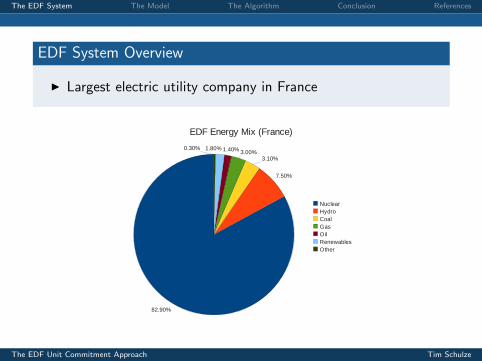
EDF System Overview

I Largest electric utility company in France



EDF System Overview

I 58 nuclear units and 47 other thermal units (coal, gas, oil)

I 50 hydro valleys: interconnected reservoirs (150) and hydroplants (448)

I Wind, solar and biomass < 2% but significantly growing

The day-ahead model has 48h in half-hour periods (96 periods)



EDF System Overview

1. Data collection finished, optimization timeframe of 15 min

2. Human postprocessing of schedules

3. Grid operator and engineers on site prepare for operation

4. Schedule is active, hourly intra-day reoptimization with atmost 30 changes in total, 3h ahead



Model for Thermal Units (incl. Nuclear)

1. Output bounds, min up/down times

2. Discrete output levels, ramp rates

3. Min const. time after increase and variation prohibition afterdecrease

4. Startup and shutdown curves

5. Daily limits on variation, startup, shutdown

6. IP instead of MIP, so as to be solved by DP



Model for Hydro Valleys

1. Turbines discharge water from upstream reservoirs, some canpump

2. The plants’ turbines are modeled individually, with fixedoutput (approx.)

3. Discrete output levels for plants, turbines ranked according topower rates (sequence constraint)

4. A plant can either produce or pump, with 30min pause inbetween

5. A turbine has to be switched (on/off) for at least 1h

6. There are plant-wide ramp rates

7. Preservation constraints balance the water flow, objective isthe value of water



Abstract Model of the Whole System

min(pi ,ri )∈Pi

∑i∈I

ci (pi )

s.t.∑i∈I

pit = Dt , ∀t ∈ T∑i∈I

rit ≥ Rt , ∀t ∈ T

Notation

I – units (gens,valleys) pi – output schedule (all t ∈ T )T – planning horizon ri – reserve (all t ∈ T )Pi – feasible schedules Dt – demandRt – required reserve



The Solution Method

I APOGEE solver, proprietary software developed 1993 under A.Renaud, later modified by C. Lemarechal

I Based on Lagrangian decomposition of the system into

1. Individual thermal units2. Individual hydro valleys (multiple plants, turbines, reservoirs)

I Solve the Lagrangian by Uzawa type subgradient methods (innew version: bundle methods)



The Primal

min(pi ,ri )∈Pi

Xi∈I

ci (pi )

s.t.Xi∈I

pit = Dt , ∀t ∈ T

Xi∈I

rit ≥ Rt , ∀t ∈ T

A Lagrangian Dual

maxλ free, µ≥0

min(pi ,ri )∈Pi

Xi∈I

ci (pi ) +Xt∈T

λt

Dt −

Xi∈I

pit

!+Xt∈T

µt

Rt −

Xi∈I

rit

!

I Inner problem separable by generation units / valleys

I Thermal unit subproblems solved by DP, hydro valley solutionsapproximated by LP (simplex method)

I Outer problem can be solved by subgradient method



Uzawa’s Subgradient Method

Initialize k = 1, λ = µ = 0 and a tolerance δ > 0. Choose sequences`εkp´k∈N

and`εkr´k∈N with

P∞k=0 ε

k =∞ andP∞

k=0

`εk´2<∞.

1. For all i ∈ I solve min(pi ,ri )∈Pi

ˆci (pi )−

Pt∈T λ

kt pit −

Pt∈T µ

kt rit˜

to find

pk+1i and r k+1

i .

2. Update λk+1t = λk

t + εkp`Dt −

Pi∈I pk+1

it

´.

3. Update µk+1t = max

˘µk

t + εkr`Rt −

Pi∈I r k+1

it

´, 0¯

.

4. If‚‚λk+1

t − λkt

‚‚2< δ and

‚‚µk+1t − µk

t

‚‚2< δ terminate. Otherwise set

k = k + 1 and go to 1.



A Variable Metric Bundle MethodInitialize k = 1 and λ1 = µ1 = λ = µ = 0 and p1, r1. Choose a penalty s > 0 and tolerance δ > 0.

1. For all i ∈ I solve min(pi ,ri )∈Pi

hci (pi )−

Pt∈T λ

kt pit −

Pt∈T µ

kt rit

ito find pk+1

i and rk+1i .

2. If L(pk+1, rk+1, λk , µk ) > L(pk , rk , λk , µk ) set λ = λk ,µ = µk and increase s. Else decrease s.

3. To find λk+1t and µk+1

t , solve

max r − 12s‖λ− λ‖2

2 −12s‖µ− µ‖2

2

s.t. r ≤ L(pl, r l, λ

l, µ

l ) + λT (Dt −

Xi∈I

plit ) + µ

T (Rt −Xi∈I

r lit ), ∀l = 1, . . . , k

µ ≥ 0

4. If‚‚‚ropt − L(pk+1, rk+1, λk+1, µk+1)

‚‚‚2< δ terminate. Otherwise set k = k + 1 and go to 1.



Why it fails.

I Primal problem is nonconvex → duality gap is nonzero

I Subgradient method: solving the dual yields no primal point

I Bundle method: After convergence of the dual, the primalpoint is noninteger

I This convex combination of schedules (think CG in theprimal!) is called pseudo schedule

I For hydro valleys only the LP relaxation is solved



How to proceed.

Use the dual solution as lower bound and perform a heuristicsearch for a primal solution.

APOGEE:

1. Solve the dual to obtain a pseudo schedule and a lowerbound. Formerly by subgradients, more recently by a bundlemethod. Solve subproblems by DP (thermal) and LP (hydro).

2. Primal recovery: perform an augmented Lagrangian basedheuristic search for primal feasible solutions. Solvesubproblems by DP (thermal) and IP heuristics (hydro).



Phase 2: Augmented Lagrangians

Consider the convex split variable problem (J1, J2 differentiable, U ∩ V 6= ∅)

minu∈U, v∈V

J1(u) + J2(v) s.t. u − v = 0.

Its augmented Lagrangian

L(u, v , λ) = J1(u) + J2(v) + λT (u − v) + c2

(u − v)T (u − v)

is not separable due to the quadratic term. However, with a maximizing price λthe primal minimization yields a feasible solution.Idea: make quadratic term separable by linearizing it.



An Auxiliary Problem

Consider the convex problem (with l1 differentiable, l2 l.s.c.)

minx∈X

l1(x) + l2(x).

The auxiliary function at a given point x ∈ X with some strongly convex,differentiable K [e.g. K(x) = 1

2xT x ] and ε > 0 is

G x(x) := 1εK(x)− 1

εxTK ′(x) + xT l ′1(x) + l2(x).

Lemma (Auxiliary Problem Principle), Proof in [1]Assume that x minimizes G x :

G x(x) = minx∈X

G x(x),

thenl1(x) + l2(x) = min

x∈Xl1(x) + l2(x).



Auxiliary Problem for the Augmented Lagrangian

We can apply this to the Lagrangian

L(u, v , λ) = J1(u) + J2(v) + λT (u − v)| {z }l2(u,v)

+ c2

(u − v)T (u − v)| {z }l1(u,v)

to get a separable auxiliary function

G (uk ,vk )(u, v) := 1εK1(u)− 1

εuTK ′1(uk) + [λ+ c(uk − v k)]Tu + J1(u)

+ 1εK2(v)− 1

εvTK ′2(v k)− [λ+ c(uk − v k)]T v + J2(v)



The Algorithm

Initialize k = 1 and λk , uk , v k , a tolerance δ > 0 and a steplength 0 < ρ < 2c.

1. uk+1 = argminu∈Uˆ

1εK1(u)− 1

εuTK ′1(uk) + [λk + c(uk − v k)]Tu + J1(u)

˜2. v k+1 = argminv∈V

ˆ1εK2(v)− 1

εvTK ′2(v k)− [λk + c(uk − v k)]T v + J2(v)

˜3. λk+1 = λk + ρ(uk+1 − v k+1)

4. If‚‚uk+1 − v k+1

‚‚2< δ stop. Otherwise set k = k + 1 and go to 1.

The choice for K1,2(·) is K(x) := εK c‖x‖2.



The Split Variable Unit Commitment Problem

minXi∈I

ci (pi )

s.t.Xi∈I

qit = Dt , ∀t ∈ T

Xi∈I

sit ≥ Rt , ∀t ∈ T

(pi , ri ) ∈ Pi

pit = qit , ∀t ∈ T , i ∈ I

rit = sit , ∀t ∈ T , i ∈ I

I qi and si satisfy the static constraints (demand, reserve)

I pi and ri satisfy the dynamic constraints (technical, temporal)

I the linking constraints need to be relaxed to achieve separability by units

I apply the augmented Lagrangian based decomposition heuristic to solvethis problem



The Phase 2 AlgorithmInitialize k = 1 and λk , µk from Phase 1 and choose a tolerance δ > 0

1. For all i ∈ I find pk+1i , rk+1

i by solving

min(pi ,ri )∈Pi

24ci (pi )−Xt∈T

“λ

kitpit + µ

kit rit

”+ Kc

Xt∈T

“(pit − pk

it )2 + (rit − rkit )2”35

2. For all t ∈ T find qk+1t , sk+1

t by solving

minqit ,sit

24Xi∈I

“λ

kitqit + µ

kit sit

”+ Kc

Xi∈I

“(qit − qk

it )2 + (sit − skit )2”35

s.t.Xi∈I

qit = Dt ,Xi∈I

sit = Rt .

3. Set λk+1it = λk

it + c(qk+1it − pk+1

it ) and µk+1it = µk

it + c(sk+1it − rk+1

it ).

4. If‚‚‚qk+1

it − pk+1it

‚‚‚2< δ and

‚‚‚rk+1it − sk+1

it

‚‚‚2< δ stop. Otherwise set k = k + 1 and go to 1.

Here the shifted duals are λkit = λk

it + c(qkit − pk

it ) and µkit = µk

it + c(skit − rk

it ).



Performance

I In operational practice phases 1 and 2 require ≈10 min

I Due to nonconvexity the final schedule satisfies load balance onlyapproximately

I The final gap is ≈3%

I Marginal costs are taken from the phase 1 solution

EDF in the Future

I MIP for hydro subproblems in phase 1 (currently LP in phase 1 and heur.in phase 2)

I Get meaningful marginal costs from phase 2

I Improve phase 2: better heuristics (gen. alg.) to reduce the gap



G. Cohen.Optimization by decomposition and coordination: A unifiedapproach.IEEE Transactions on Automatic Control, 1978.

L. Dubost, R. Gonzalez, and C. Lemarechal.A primal-proximal heuristic applied to the french unitcommitment problem.Mathematical Programming, 2005.

G. Hechme-Doukopoulos, S. Brignol-Charousset, J. Malick,and C. Lemarechal.The short-term electricity production management problem atEDF.OPTIMA 84 Mathematical Optimization Society Newsletter,2010.



A. Renaud.Daily generation management at Electricite de France: Fromplanning towards real time.IEEE Transactions on Automatic Control, 1993.



The EDF Day Ahead Unit Commitment Approach

Scheduling a la Francaise – It’s all French to me!

School of Mathematics


the edf day ahead unit commitment · pdf filethe edf systemthe modelthe...

Documents