The Economics of Water Project Capacities and Conservation Technologies

Yang Xie David Zilberman

Department of Agricultural and Resource Economics

University of California, Berkeley

phd.yang.xie@gmail.com zilber11@berkeley.edu

Selected Paper prepared for presentation at the Agricultural & Applied Eco-

nomics Association’s 2014 AAEA Annual Meeting, Minneapolis, MN, July

27–29, 2014

Copyright 2014 by Yang Xie and David Zilberman. All rights reserved. Readers may

make verbatim copies of this document for non-commercial purposes by any means, provided

that this copyright notice appears on all such copies.

The Economics of Water Project Capacities andConservation Technologies∗

Yang Xie† David Zilberman‡

May 26, 2014

Abstract

This paper builds a model determining optimal capacities of diversion dams or wa-ter transfer projects. The model incorporates stochastic inflows to the dams and therole of the dam capacity in reducing overflows, and gives a closed-form expression ofthe marginal benefit of capacities. Comparative static analysis suggests that largerwater projects could be required by 1) improvements in water management efficiency,2) upward shifts in the marginal overflow-caused loss, or 3) more abundant inflows.The result provides important policy implications about the impact of integrated wa-ter reforms, rising concern about food security, and climate change on optimal waterproject capacities. The model is also applied to analyze the relation between waterproject capacities and conservation technologies, showing 1) that too large or too smallwater projects could discourage adopting conservation technologies, 2) that the impactof conservation technologies on optimal capacities is ambiguous, and 3) that if design-ers of water projects take water users’ potential adoption of conservation technologiesinto account, the first-order condition of the capacity determination model could havemultiple solutions.

∗This paper is prepared for the Agricultural and Applied Economics Association 2014 Annual Meetingat Minneapolis, MN, on July 27–29, 2014. We thank the three anonymous reviewers for their valuablecomments.

†Corresponding author. Affiliation: Department of Agricultural and Resource Economics, University ofCalifornia at Berkeley. Address: 207 Giannini Hall, University of California, Berkeley, CA 94720-3310, U.S.Email: phd.yang.xie@gmail.com.

‡Affiliation: Department of Agricultural and Resource Economics, University of California at Berke-ley. Address: 207 Giannini Hall, University of California, Berkeley, CA 94720-3310, U.S. Email: zil-ber11@berkeley.edu.

1 Introduction

Water is arguably the most important natural resource in social, economic, and political

development, and eventually, the source of life and death. Water is subjected to large

variability and special inequality, however, both across time and between regions. The

variability and the inequality make water the focal issue in world and local cooperation and

conflicts, and to overcome the variability and the inequality, people build dams, reservoirs,

canals, and other water projects to store, release, and transfer water intertemporally and

interregionally.

Stabilization and improved allocation of water justify investments in water projects, since

they provide agricultural, industrial, environmental, and other social-economic benefits to

society. Yet, building large water projects also incurs enormous cost in construction, mainte-

nance, and environmental externality. Moreover, the benefit and the cost are not distributed

equally among regions and people, so in both developed and developing countries, large

water projects are always not only economically significant, but also politically sensitive.1

Motivated by political considerations, water projects have been major public work, but

not always justified on the ground of economic efficiency. Realizing it, international organi-

zations recommend to establish cost-benefit criteria to evaluate water projects and determine

their optimal capacities. This area has therefore seen the flourish of the cost-benefit analysis

method. The success of the method has been symbolized by the Principles and Guidelines

(1983) of the United States. As recognized in Zilberman et al. (1994), however, one major

critique of the method and the Principles and Guidelines is that they lead to the design

of water projects that overemphasizes “hard” engineering solutions, ignoring the problem-

solving capacities of “soft” management and institutional solutions. The critique has also

been highlighted in the recent California drought and the related policy discussions, as the

expansion of water project capacities and the policies encouraging conservation and recy-

cling are competing bitterly for limited policy resources.2 In this paper, we develop a new

1A controversial term hydraulic civilizations is coined by historian Wittfogel (1957), associating theauthoritarian regime in East Asia with the large-scale public water projects in the area. Fischhendler andZilberman (2005) discuss the political implications of the United States Central Valley Project ImprovementAct of 1992. Duflo and Pande (2007) examine the productivity and distributional effects of large irrigationdams in India. For other examples, see McCully (2001) and Singh (2002). Among others, recent and ongoingexamples are about the series of dams in the Amazon Basin in South America and along the Yangtze River inChina, with the Belo Monte Dam in Brazil and the Three Gorges Dam in China topping the lists, respectively.Examples of the media coverage include Kennedy (2001), Lyons (2012), The Economist (2013a, 2013b), andCheng (2014), among others. Jackson and Sleigh (2000) detail the social-economic impacts of resettlementfor the Three Gorges Dam in China. Another ongoing example specifically about water scarcity and waterprojects is about the proposed canal from the Paraıba do Sul to the Cantareira Water System, initiated bythe Governor of Sao Paulo, Brazil. For media coverage, see Carvalho (2014) and de Arauo (2014a,b).

2On the one hand, several bills have been introduced to the Congress to authorize and fund expansion of

1

analytical framework for the design of water projects, incorporating rising concerns about

climate change, resource conservation, and water-provided food, energy, and environmental

amenities. The framework provides insights about the implications of the changes in the in-

stitutional, environmental, and technological conditions on optimal water project capacities.

The framework is founded on a stylized model for the optimal capacity determination of

a dam. The dam sits upstream, gathers inflows in wet seasons, and releases all the gathered

water downstream in dry seasons, generating agricultural, industrial, and environmental ben-

efits. The model incorporates stochastic inflows to the dam and the role of the dam capacity

in reducing overflows, and the incorporation is done in such a simple way that we can find

a closed-form expression of the marginal benefit of dam capacities. The comprehensiveness

and the simplicity establish the novelty of our model with respect to literature (e.g. Tsur

(1990), Fisher and Rubio (1997), and Schoengold and Zilberman (2007, p.2943,2955)).

Our model links the marginal benefit of dam capacities to the benefit of water releases,

and takes into account the inflow distribution and the losses caused by overflows. This

feature allows our framework to obtain major conceptual results with implications to ma-

jor policy problems, about water project capacities, water allocation institutions, tradeoffs

among alternative water-dependent services, water distribution systems, climate change,

resource conservation, and the relation among them. We believe that the importance and

variety of the results, implications, and insights will allow rich discussions and investigations.

The first category of the insights comes from the comparative static analysis around the

water release benefit, which suggests that many improvements in water management effi-

ciency could lead to larger optimal capacities of water projects. We find conditions under

which institutional reforms, technological reforms, and reduced concentration of water al-

location will affect optimal dam capacities. We discuss four improvements as examples of

the implications, which are 1) reforming water rights to water markets, which, for example,

has been encouraged in the western United States by the Central Valley Project Improve-

ment Act of 1992, 2) reallocating water from irrigation to hydropower or environmental

sectors in the age of rising energy prices, which has been discussed in literature, for example,

about Australia’s Murray–Darling Basin, 3) optimally centralizing conveyance investments,

water storage and conveyance capacities, including at least the California Emergency Drought Relief Act of2014, the Upper San Joaquin River Storage Act of 2014, the Shasta Dam Expansion Act of 2014, the SanLuis Reservoir Expansion Act of 2014, the Sacramento Valley Water Storage and Restoration Act of 2014,and the Sacramento–San Joaquin Valley Emergency Water Delivery Act of 2014. Californian lawmakers havealso been discussing issuing water bonds to finance more water projects. On the other hand, there are alsovoices suspecting the usefulness of increasing capacities and requiring more funding for recycling projectsand conservation technology adoption. Examples of discussions on the recent Californian water policy issuesinclude Calefati (2014), Feinstein (2014b,a), Freking (2014), Garamendi (2014a,b), and Nirappil (2014),among others.

2

which has been analyzed in Chakravorty et al. (1995), and 4) weakening the market power

of monopsony, like the Water Users Associations in the United States, in water generation

markets, which has been discussed in Chakravorty et al. (2009). The discussion can be

generalized to a framework suggesting that integrated improvements in water management

efficiency, for example the Central Valley Project Improvement Act, could optimally require

more or larger water projects. The implication contrasts the cost-minimization logic which

predicts smaller water projects under higher efficiency of water distribution, allocation, use,

and management.

The second category of the insights emerges with the comparative static analysis around

the loss caused by overflows. We show that larger dams are needed if the marginal over-

flow loss increases. The analysis contributes to literature, since economic models about

dam capacity determination rarely present explicit impacts of the overflow loss on optimal

capacities. The analysis also suggests that if the marginal overflow loss is positively corre-

lated with economic growth, then economic growth could require larger capacities of water

projects, and that if the economic loss caused by overflow-interrupted food supply is more

seriously concerned, especially in the age emphasizing food security, then larger capacities

of water projects could be needed.

The comparative static analysis around the inflow distribution provides the third category

of the insights. We show that if the inflow to the dam is more abundant in both dry and wet

years, or more precisely, has its distribution shifted to the right in a first-order dominating

way, then the dam could be optimally larger. This result contributes to the literature about

the impact of climate change on optimal capacities of water projects, examples of which

include Fisher and Rubio (1997), among others. Different to Fisher and Rubio (1997), who

focus on the impact of variability of inflows, we focus on the impact of the general abundance

of the inflows. This result implies that if warming makes water more abundant in the source

area of water transfer programs, the programs might optimally need to prepare larger transfer

capacities. The implication is practically important, since the scenario of warming-caused

inflow change might not be too wild for some large, important water transfer programs,

for example the California State Water Project and China’s South–North Water Transfer

Project.

Last but not least, our model insights about the relation between dam capacities and

conservation technologies, which, to our knowledge, hasn’t been systematically analyzed in

literature. In this paper, we analyze the relation in a framework where a dam capacity

decision and a technology adoption decision are to be made respectively by a dam designer

and a representative water user.3 We characterize conservation technologies as rotating

3Readers can regard the approach as a simplified integrated watershed management, which incorporates

3

clockwise the marginal water release benefit function. This characterization is consistent with

that in Caswell and Zilberman (1986) and some other literature. With the characterization,

we analyze the relation from the following three perspectives:

Impacts of dam capacities on conservation technology adoption Though public

water projects usually affect a large number of water users and potential adopters, they are

almost ignored in the literature that studies factors affecting conservation technology adop-

tion.4 We fill the gap by showing a non-monotonic impact of dam capacities on the incentive

of adopting conservation technologies. This impact suggests that too large or too small dams

could discourage adopting conservation technologies. This result is also consistent with the

studies that finding a non-monotonic relation between resource abundance and conservation

technology adoption: on the one hand, more abundant water or resource availability substi-

tutes the need of conservation; on the other hand, having too little water or resource leaves

too little room for conservation technologies to aggregate their marginal-benefit advantage

over existing technologies to cover the fixed adoption cost.

Impacts of conservation technologies on optimal dam capacities The comparative

static analysis of our capacity determination model shows that the impact of conservation

technology adoption on optimal dam capacities is ambiguous, and depends on the dam

capacity with existing technologies. Compared with the literature on capacity determination,

which includes Tsur (1990), Fisher and Rubio (1997), Schoengold and Zilberman (2007,

p.2943,2955), and others, it is novel that we identify conservation technology adoption as

a potential factor affecting the dam capacity decision. The result also contrasts the cost-

minimization logic in capacity determination, which would unambiguously predict a smaller

dam with conservation technologies.

Impacts of potential adoption of conservation technologies on optimal dam ca-

pacities We consider another setting in which the dam designer recognizes that her dam

capacity decision would affect water users’ technology adoption decision, and would then

affect the benefit of the dam. Different to the literature like Zhao and Zilberman (2001)

that focuses on the option value and optimal timing of resource development, our setting

makes the potential adoption create a discontinuous marginal benefit of dam capacities. The

discontinuity potentiates multiple solutions to the first-order condition of the capacity deter-

mination model, making the dam capacity problem not only more complicated, but also more

decision-making at different levels of water systems.4We shall discuss the literature in more detail in Section 4.

4

interesting. The analysis also suggests that one reason for oversized water projects could be

the designer’s overlooking of the future potential adoption of conservation technologies.

The paper is unfolded as follows. Section 2 builds and solves the model for optimal

dam capacity determination. Section 3 analyzes the comparative statics of the model, and

presents theoretical and practical implications of the analysis. Section 4 analyzes the relation

between dam capacities and conservation technologies. Section 5 concludes the paper with

summary and directions for extensions and further research.

2 An optimal dam capacity problem and its solution

In this Section we build a model for the determination of optimal dam capacities. In each

period t, water of stochastic amount et flows into the dam of a capacity w, and then the dam

releases water of amount wt into a distribution and allocation system. As the economics of the

distribution and allocation system has been discussed in detail in Chakravorty et al. (1995)

and Chakravorty et al. (2009) and isn’t our paper’s main focus, we leave the functioning of

the system out of the model.

In our model, the water release is determined by the following Assumption.

Assumption 1 (Water release determination). The dam capacity caps the maximum amount

of the release: wt = min {et, w}.

Assumption 1 means that in each period, the dam cannot hold more inflow than how much

its capacity allows, and the dam releases all of the held. Readers can regard the dam as a

diversion dam or water transfer project which sits upstream, gathers inflows in wet seasons,

and releases all the gathered water downstream in dry seasons, generating agricultural,

industrial, environmental, and ecological benefits. For simplicity, we don’t consider the

intertemporal water inventories in the dam. In a concurrent paper, Xie and Zilberman

(2014) build and analyze a parallel model which incorporates the optimal management of

water inventories.

In each period, the benefit of the dam includes the benefit generated by the water release,

Bt(wt), net of the loss caused by overflows from the dam, Lt(max {et, w}− w).5 This setting

completes the water system with the dam, as illustrated in Figure 1.

Before the dam is built, its designer recognizes the construction and maintenance cost,

C(w), and the environmental damage cost, D(w). The properties of the benefit, the loss,

and the cost functions are formalized by the following Assumption.

5For simplicity we don’t model each of the elements of the benefit and the loss in detail, which could bea direction for future research.

5

Figure

1:A

water

system

withadam

6

Assumption 2 (Function properties). The marginal water release benefit is non-negative

and decreasing: B′t(·) ≥ 0 and Bt

′′(·) < 0. The overflow loss is zero when there is no overflow,

it is positive when there is an overflow, and the marginal overflow loss is positive and weakly

increasing: Lt(0) = 0, Lt(·) > 0 elsewhere, Lt′(·) > 0, and Lt

′′(·) ≥ 0. The marginal

construction and maintenance cost is positive and increasing: C ′(·) > 0 and C ′′(·) > 0. The

marginal environmental damage cost is positive and increasing: D′(·) > 0 and D′′(·) > 0.

Assumption 2 isn’t very unrealistic. For example, the water release benefit depends on

the design of the distribution system, the pricing scheme of water, the institution of water

allocation, the efficiency of water application, and many other things, but most importantly,

the marginal benefit of water should be much higher when it is scarce than when it is

abundant, so a decreasing marginal water release benefit is reasonable; huge overflows weaken

the economy’s ability to react to additional overflows, so the marginal overflow loss should be

weakly increasing; resource of dam building and maintenance is always limited, so assuming

increasing marginal construction and maintenance cost isn’t too wild; larger dams make

the ecological system more vulnerable to further human actions, so it is fair to assume

an increasing marginal environmental damage cost.6 Furthermore, as we shall see later,

Assumption 2 makes our optimal dam capacity problem, which is formalized by the following

Assumption, have solutions.

Assumption 3 (The social planner’s problem with a discount factor). A social planner

chooses the dam capacity to maximize the discounted expected sum of water release benefits

minus overflow losses, net of the construction, maintenance, and environmental cost of the

dam. The discount factor ρ ∈ (0, 1).

With Assumptions 1 and 2, Assumption 3 presents the optimal dam capacity problem:

maxw≥0

E0

[∞∑s=0

ρs (Bs(min {es, w})− Ls(max {es, w} − w))

]− C(w)−D(w). (1)

For technical simplicity, we propose another two Assumptions.

Assumption 4 (Stationary water release benefits and overflow losses). The water release

benefit function is the same across time: Bt(·) = B(·) for any t. The overflow loss function

is the same across time: Lt(·) = L(·) for any t.

Assumption 5 (Inflows i.i.d.). The stochastic inflow is identically and independently dis-

tributed as e, with the cumulative distribution function F (·) and the probability density func-

tion f(·), where F ′(·) = f(·).6The environmental damage of dams could be correlated with how water releases are used. In this model

we model the environmental damage that is related to water releases into the water release benefit function.

7

The two Assumptions suggest that we ignore trends in the water release benefit, the

overflow loss, and the inflow. They turn the optimal dam capacity problem into

maxw≥0

1

1− ρE [B(min {e, w})− L(max {e, w} − w)]− C(w)−D(w), (2)

which is equivalent to

maxw≥0

1

1− ρ

[∫ w

−∞B(e)f(e)de+ (1− F (w))B(w)

]+

(− 1

1− ρ

∫ ∞

w

L(e− w)f(e)de

)− C(w)−D(w).

(3)

In the objective function, the first term is the discounted expected sum of water release

benefits, and the second term is the negative discounted expected sum of overflow losses.

The two terms form the benefit of the dam. The third and the fourth terms form the cost

of the dam. By Leibniz’s integral rule, the marginal values of the discounted expected sum

of water release benefits and the negative discounted expected sum of overflow losses with

respect to dam capacities are

1

1− ρ(1− F (w))B′(w) > 0 and

1

1− ρ

∫ ∞

w

L′(e− w)f(e)de > 0, (4)

respectively. The first-order condition of the problem is then

1

1− ρ(1− F (w))B′(w) +

1

1− ρ

∫ ∞

w

L′(e− w)f(e)de = C ′(w) +D′(w). (5)

The left-hand side of the condition is the marginal benefit of dam capacities, which

depends on the water release benefit function, the overflow loss function, and the inflow

distribution. The right-hand side is the marginal cost of dam capacities. Assumptions 2, 4,

and 5 guarantee that the marginal benefit is decreasing and the marginal cost is increasing,

so the root of the first-order condition, w∗, helps the objective function to reach its maximum

but not minimum.7

The root is the solution to the optimal dam capacity problem if and only if the root is

nonnegative. Otherwise, the model might have a corner solution, which is a capacity of zero.

7The first term in the marginal benefit is the product of a positive constant and two positive, de-creasing functions, so it is decreasing in w. The second term is the product of a positive constantand an positive integral. The integral is decreasing in w, since its derivative with respect to w is− 1

1−ρ

[L′(0)f(w) +

∫∞w

L′′(e− w)f(e)de], which is negative. The second term is then also decreasing in

w. The marginal benefit is then increasing in w. The marginal cost is the sum of two positive, increasingfunctions, so it is decreasing in w.

8

Zero capacities could happen when the marginal cost of dam capacities is already larger

than the marginal benefit when the capacity is zero. It is also possible that the first-order

condition has no root. In this case, the marginal cost of dam capacities is always smaller

than the marginal benefit, and the solution to the problem is an infinite capacity. As the

zero-capacity and the infinite-capacity cases add little intuition to our further analysis, we

rule them out by the following Assumption.

Assumption 6 (Finite, interior solutions). The marginal benefit of dam capacities is larger

than the marginal cost when the capacity is zero, while smaller when the capacity is large

enough.

Since Assumption 2 provides monotonicity and continuity for all the functions, Assump-

tion 6 means there is always a unique, finite, and positive root of the first-order condition,

which solves the optimal dam capacity problem.8

All the Assumptions and the analysis proves the following Proposition, the main result

of this Section.

Proposition 1 (The model’s solution). Under Assumptions 1, 2, 3, 4, 5, and 6, the optimal

dam capacity w∗ makes the marginal benefit dam capacities equal to the marginal cost. Math-

ematically, w∗ solves Equation (5). Graphically, w∗ makes the decreasing marginal benefit1

1−ρ(1− F (w))B′(w) + 1

1−ρ

∫∞w

L′(e − w)f(e)de intersect with the increasing marginal cost

C ′(w) +D′(w).

Proposition 1 characterizes the solution to our model, a model with minimal but still

necessary complication. Literature has proposed several models about optimal determina-

tion of water project capacities. Almost all of the models carry minimal and necessary

complication for their own purposes, but are generally either too simplified, unnecessarily

complicated, or too general for our purpose. For example, Schoengold and Zilberman (2007,

p.2943) model the marginal benefit of dam capacities in a static, black-box style, which is

sufficient for their focus on the logic of oversized water projects, but might be difficult to

proceed with further serious analysis and implications. In the same Chapter, Schoengold

and Zilberman (2007, p.2955) also try to improve the model by incorporating water demand

uncertainty and simplifying water release as the dam capacity. They stop their analysis after

deriving the first-order condition, based on the intensive simplification. They also ignore the

stochastic inflows and the role of the dam capacity in reducing overflows, so the improved

model does extend their story to the case with water demand uncertainty, but might help

8For the readers who might think corner solution should be emphasized in the optimal dam capacityproblem, it could be helpful if we regard the dam capacity in our model as the storage capacity of a hugewater system, in which a new dam only means a small increase in the storage capacity.

9

little to analyze the impact of the inflow distribution and the overflow loss on optimal dam

capacities. Tsur (1990) discusses the optimal capacity of a groundwater project as a buffer

of uncertain supply of surface water, but the inflow to the groundwater project is still as-

sumed deterministic, so the model serves well as a contribution to the idea of conjunctive

use of groundwater and surface water, but might help little to examine the impact of the

inflow distribution.9 As in Burt (1964, 1966, 1967, 1970), Tsur and Graham-Tomasi (1991),

Truong (2012), and many other papers, the literature that incorporates stochastic inflows

or dynamic control focuses on the optimal control rule of water releases or inventories, but

at the same time, largely increases the difficulty in finding closed-form expressions of the

marginal benefit of dam capacities. It is then difficult to analyze comparative static effects

on dam capacities in the models. An admirable attempt by Fisher and Rubio (1997) finds

a closed-form expression, but their continuous-time dynamic control of both the water in-

ventory and the storing capacity, at the other extreme, is more than what we need in this

paper. Moreover, their model focuses on the impact of the variability of the stochastic in-

flows instead of that of the whole distribution, and doesn’t explicitly characterize the dam’s

function in controlling the overflow loss. In more general settings, Arrow and Fisher (1974)

and Zhao and Zilberman (1999, 2001), among others, focus on the general option value and

optimal timing of environmental restoration investment. Their treatment is out of the scope

of this paper.

Contributing to the literature, our model incorporates stochastic inflows and overflow

losses simultaneously, and is still so simplified that we can find the closed-form expression

of the marginal benefit of dam capacities, without much loss in intuition. The closed-form

expression clearly shows the dependency of the marginal benefit on the inflow distribution,

the water release benefit function, and the overflow loss function. This feature allows us to

minimize the complication in comparative statics, and provide implications to answer many

important, theory- and policy-relevant questions about water project capacities, water allo-

cation institutions, tradeoffs among alternative water-dependent services, water distribution

systems, climate change, resource conservation, and the relation among them. We shall show

the comparative statics and the implications in following Sections.

3 Comparative static analysis

In this Section we analyze the comparative statics of the capacity determination model

around the water release benefit function B(·), the overflow loss function L(·), and the

distribution of the stochastic inflow, which is represented by F (·). The analysis provides

9Reducing overflows isn’t applicable to groundwater projects.

10

important policy implications about the impact of water management efficiency and climate

change on optimal capacities of water projects. Appendix A presents the comparative statics

around the construction, maintenance, and environmental damage cost functions, which is

more straightforward and less interesting.

3.1 The impact of the water release benefit

We exhibit the impact of the water release benefit function on optimal dam capacities by

the following Proposition.

Proposition 2 (The impact of the water release benefit). Under Assumptions 1, 2, 3, 4, 5,

and 6, if the marginal water release benefit function shifts up, then the optimal dam capacity

becomes larger. Mathematically and more precisely, consider two functions of the water

release benefit, B1(·) and B2(·), and the corresponding optimal dam capacities, w∗1 and w∗2.

If B2′(·) ≥ B1′(·), then w∗2 ≥ w∗1.

As mentioned in Section 2, Xie and Zilberman (2014) extend Proposition 2 to the case

with optimal water-inventory control. Figure 2 graphically illustrates the intuition of Propo-

sition 2. In the Figure, upward shifting B′(·) shifts up the marginal benefit of dam capacities.

Since the marginal benefit of dam capacities intersects with the marginal cost from above,

their intersection moves to the right. By Proposition 1, the optimal dam capacity increases.

Though apparently straightforward, Proposition 2 contributes to literature, since to our

knowledge, not much literature emphasizes the comparative analysis about capacity deter-

mination around the water release benefit function. For example, among papers that are

specifically about capacity determination, Schoengold and Zilberman (2007, p.2943,2955)

don’t analyze comparative statics. Tsur (1990) mentions that larger uncertainty in surface

water supply suggests a higher value of groundwater projects, but the paper doesn’t empha-

size whether the groundwater project capacity should be larger. Tsur (1990) does discuss

the comparative statics of capacities around cost functions, but not around benefit functions.

Proposition 2 can provide important policy implications, since many improvements in

water management efficiency could shift up the marginal water release benefit function.

For example, we analyze four improvements, which are reforming water rights to water

markets, reallocating water from irrigation to hydropower or environmental sectors in the

age of rising energy prices, optimally centralizing conveyance investments, and weakening

the market power of monopsony in water generation markets. By Proposition 2, all the four

improvements could encourage larger dams.

11

B2′(·) ≥ B1′(·) ⇒ w∗2 ≥ w∗1

Figure 2: The impact of the water release benefit on the optimal dam capacity

Transitions from water rights to water markets Much literature recognizes that

reforming a traditional water right system to market-like water allocation can improve water

use efficiency, including Burness and Quirk (1979), Gisser and Sanchez (1980), Gisser and

Johnson (1984), Howe et al. (1986), Chakravorty et al. (1995), Dinar and Tsur (1995), and

Brill et al. (1997), among others. Good surveys about the topic include Saleth and Dinar

(2000), Zilberman and Schoengold (2005), Chong and Sunding (2006), and Tsur (2009). As

one example of the traditional systems, in the queuing system used in the western United

States before the Central Valley Project Improvement Act of 1992, the seniority of water

rights is determined by historical water use in irrigation, and water is priced by the average

cost. As argued in Zilberman and Schoengold (2005), in this system, “trading bans and

low water prices do not provide the owners of senior rights with the incentive to adopt

water conserving technologies to reduce their water use and sell the extra water to highly

efficient individuals with junior or no water rights.” The Central Valley Project Improvement

Act, however, allows water users to sell some of their water rights in a water market. The

transition from water rights to water markets includes the high willingness-to-pay of the

highly efficient individuals for additional water into the marginal water-use benefit, and has

water priced by the marginal cost instead of the average cost. The two improvements expand

the marginal water-use benefit, and then shift up the marginal water release benefit.10 By

10This argument is formalized in Appendix D.

12

Proposition 2, we have the following Implication about the impact of the transition on

optimal dam capacities.

Implication 1. Transitions from water rights to water markets could require larger capacities

of water projects.

Rising energy prices and reallocation of water from irrigation to hydropower or

environmental sectors In the age of rising energy prices, increasing water provision for

hydropower could gain extra water release benefit. Hydropower is cleaner than fossil fuels, so

the gain could also occur in the environmental sector. Released water could also help down-

stream areas to resist saltwater from intruding, protect endangered species, and therefore

improve the quality of water and environment. Following this idea, much literature recog-

nizes that reallocating water use from agricultural sector to hydropower or environmental

sectors could improve water management efficiency and shift up the marginal water release

benefit, including Chatterjee et al. (1998), Quiggin (2006), Schoengold et al. (2008), and

Truong (2012), among many others. For example, about the case of the Murray–Darling

Basin, Australia’s significant agricultural area, Truong (2012) reads, “it is now widely ac-

knowledged that the (marginal) value of water use for environmental purposes is much higher

than the (marginal) value of water use in irrigation and reallocation of water resources from

the irrigation sector to the environmental sector will significantly enhance the efficiency in

water usage (Quiggin 2006).” By Proposition 2, the upward shift in the marginal water

release benefit could lead to larger dams. The following Implication documents the impact.

Implication 2. Rising energy prices and reallocation of water from irrigation to hydropower

or environmental sectors could require larger capacities of water projects.

Optimal centralization of conveyance investments Chakravorty et al. (1995) com-

pare “a utility that supplies water to firms but fails to invest optimally in the distribution

canals” with a utility that centralizes and optimizes the investments. They discuss two pric-

ing schemes for the suboptimal utility, which are a spatially uniform pricing solution and

a water market solution, respectively. They argue that there exists a range of the level of

water release in which the marginal water release benefit with optimal conveyance invest-

ments is always higher than that with suboptimal conveyance investments. The argument

is confirmed by their simulation of water use for cotton irrigation in the western United

States. This result implies that if the water release from our dam is always within the range,

then centralizing conveyance investments will shift up the marginal water-benefit function.

By Proposition 2, the shift could encourage larger dams, as documented by the following

Implication.

13

Implication 3. Optimal centralization of conveyance investments could require larger ca-

pacities of water projects.

Weakening of the market power of monopsony in water generation markets

Chakravorty et al. (2009) compare the private Water Users Associations in the western

U.S. with the social optimal water distribution system. The Water Users Associations are

monopsonies in the water generation market, examples of which include California’s water

districts. As described in Congressional Budget Office of the United States (1997), the dis-

tricts “appropriate water, construct reservoirs and distribution systems” and buy surface

water supplies from the State or the Bureau of Reclamation. Chakravorty et al. (2009) show

that the market power of the monopsony could make the water conveyed into the distri-

bution system smaller than the social optimal level. Following this idea, when the water

release from our dam caps the maximum amount of water that is conveyed into the distribu-

tion system by the water generation market (and actually applied in economy), removing the

market power of the private Water Users Associations can weakly increase water application,

and then shift up the marginal water release benefit.11 Proposition 2 implies the following

Implication, which documents the positive impact of the shift on dam capacities.

Implication 4. Weakening of the market power of monopsony in water generation markets

could require larger capacities of water projects.

The four examples suggest a framework which analyzes the impact of improvements

in water management efficiency on optimal capacities of water projects, and gives some

empirical implications. With progresses in environmental, resource, and water economics,

major water reforms have been and will be implemented, and they could help to gain extra

water release benefit. For example, the purposes of the Central Valley Project Improvement

Act include to increase economic and environmental benefit from the Central Valley Project

through reforms in water transfers, water pricing, conservation, and wildlife restoration.12

By Proposition 2, whether and how much the reforms would lead to larger water projects

depends on whether and how much the efficiency improvements would shift up the marginal

water release benefit. The dependency asks for serious empirical analysis on the impact of

the reforms on the marginal water release benefit.

To conclude this Subsection, we discuss a little bit more about the intellectual interest-

ingness of the implications of Proposition 2. One might literally expect that improvements

in water management efficiency should mean more efficient water use, so it would require

11This argument is formalized in Appendix E.12For details about environmental impacts of the Central Valley Project Improvement Act, see United

States Department of Interior et al. (1999).

14

smaller water supply and dam capacities. This logic is found in some engineering literature,

where dam designers are minimizing cost of dams to satisfy specific engineering and policy

constraints.13 In contrast, Proposition 2 shows that weighing the marginal benefit and cost

of dam capacities, larger dams would be required. This contrast is similar to the surprise in

Chakravorty et al. (1995), where the optimal water use is larger under optimal distribution

system than that under non-optimal distribution system.

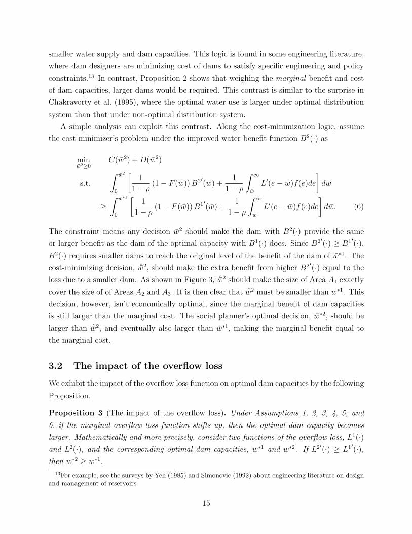
A simple analysis can exploit this contrast. Along the cost-minimization logic, assume

the cost minimizer’s problem under the improved water benefit function B2(·) as

minw2≥0

C(w2) +D(w2)

s.t.

∫ w2

0

[1

1− ρ(1− F (w))B2′(w) +

1

1− ρ

∫ ∞

w

L′(e− w)f(e)de

]dw

≥∫ w∗1

0

[1

1− ρ(1− F (w))B1′(w) +

1

1− ρ

∫ ∞

w

L′(e− w)f(e)de

]dw. (6)

The constraint means any decision w2 should make the dam with B2(·) provide the same

or larger benefit as the dam of the optimal capacity with B1(·) does. Since B2′(·) ≥ B1′(·),B2(·) requires smaller dams to reach the original level of the benefit of the dam of w∗1. The

cost-minimizing decision, ˆw2, should make the extra benefit from higher B2′(·) equal to the

loss due to a smaller dam. As shown in Figure 3, ˆw2 should make the size of Area A1 exactly

cover the size of of Areas A2 and A3. It is then clear that ˆw2 must be smaller than w∗1. This

decision, however, isn’t economically optimal, since the marginal benefit of dam capacities

is still larger than the marginal cost. The social planner’s optimal decision, w∗2, should be

larger than ˆw2, and eventually also larger than w∗1, making the marginal benefit equal to

the marginal cost.

3.2 The impact of the overflow loss

We exhibit the impact of the overflow loss function on optimal dam capacities by the following

Proposition.

Proposition 3 (The impact of the overflow loss). Under Assumptions 1, 2, 3, 4, 5, and

6, if the marginal overflow loss function shifts up, then the optimal dam capacity becomes

larger. Mathematically and more precisely, consider two functions of the overflow loss, L1(·)and L2(·), and the corresponding optimal dam capacities, w∗1 and w∗2. If L2′(·) ≥ L1′(·),then w∗2 ≥ w∗1.

13For example, see the surveys by Yeh (1985) and Simonovic (1992) about engineering literature on designand management of reservoirs.

15

Capacity w∗1 is optimal when the water release benefit function is B1(·). Capacity w∗2 isoptimal when the water release benefit function is B2(·). Capacity ˆw2 is the minimal capacityto provide the same or larger benefit with B2(·) as the dam of w∗1 with B1(·) does. Thewater release benefit functions satisfy that B2′(·) ≥ B1′(·), so ˆw2 ≤ w∗1 ≤ w∗2, and the sizeof the Areas satisfies that A1 = A2 + A3.

Figure 3: Comparison between cost minimization and economic-profit maximization

L2′(·) ≥ L1′(·) ⇒ w∗2 ≥ w∗1

Figure 4: The impact of the overflow loss on the optimal dam capacity

16

Proposition 3 is illustrated in Figure 4. Since the marginal value of the negative dis-

counted expected sum of overflow losses with respect to dam capacities is 11−ρ

∫∞w

L′(e −w)f(e)de, an upward shift in L′(·) shifts up the marginal value and therefore the marginal

benefit of dam capacities. Since the marginal benefit intersects with the marginal cost from

above, the intersection then moves to the right. By Proposition 1, the optimal dam capacity

then increases.

Though the role of dam capacities in reducing overflows is well recognized, as for example

in Green et al. (2000), economic models about dam capacity determination rarely present

explicit impacts of the overflow loss on optimal capacities. As mentioned in Section 2, the

examples include Tsur (1990), Fisher and Rubio (1997), and Schoengold and Zilberman

(2007, p.2943, 2955), among others. Proposition 3 contributes to the literature, by modeling

the role of dam capacities in reducing overflows, and showing the relation among the overflow

loss, the marginal benefit of dam capacities, and the optimal dam capacity.

Proposition 3 also gives policy implications. For example, if floods caused by overflows can

wipe out production in flooding areas, the (marginal) economic damage caused by overflows

then becomes larger as economy grows. Proposition 3 implies that larger dams are required

as economy grows. The implication is documented by the following Implication.

Implication 5. If the marginal overflow loss is positively correlated with economic growth,

then economic growth could require larger capacities of water projects.

Another example of the implications of Proposition 3 is related to the increasing concern

about food security. Overflows might seriously interrupt agricultural production by flooding

and waterlogging, and if the loss is more seriously concerned, especially in the age empha-

sizing food security, then larger capacities of water projects could be required. We conclude

this Subsection by documenting this implication by the following Implication.

Implication 6. If the marginal overflow loss is more seriously concerned in the age empha-

sizing food security, then the emphasis could require larger capacities of water projects.

3.3 The impact of the inflow distribution

By integration by parts, the marginal benefit of dam capacities

1

1− ρ(1− F (w))B′(w) +

1

1− ρ

∫ ∞

w

L′(e− w)f(e)de

=1

1− ρ(1− F (w))B′(w) +

1

1− ρ

(L′(∞)− L′(0)F (w)−

∫ ∞

w

F (e)L′′(e− w)de

). (7)

17

Since Assumption 2 requires positive B′(·) and L′(·) and nonnegative L′′(·), a downward shift

in F (·) shifts up the marginal benefit of dam capacities. This analysis proves the following

Proposition on the impact of the inflow distribution on optimal dam capacities.

Proposition 4 (The impact of the inflow distribution). Under Assumptions 1, 2, 3, 4,

5, and 6, if the inflow distribution is shifted in a first-order stochastically dominating way,

then the optimal dam capacity becomes larger. Mathematically and more precisely, consider

two cumulative distribution functions of the inflow, F 1(·) and F 2(·), and the corresponding

optimal dam capacities, w∗1 and w∗2. If F 2(·) ≤ F 1(·), then w∗2 ≥ w∗1.

F 2(·) ≤ F 1(·) ⇒ w∗2 ≥ w∗1

The probability density function f i(·) corresponds to the cumulative distribution functionF i(·), where i = 1, 2.

Figure 5: The impact of the inflow distribution on the optimal dam capacity

Proposition 4 is illustrated in Figure 5. In the Figure, a downward shift in F (·) shifts

up both the marginal values of the discounted expected sum of water release benefits and

the negative discounted expected sum of overflow losses, and then the marginal benefit of

dam capacities. Since the marginal benefit intersects with the marginal cost from above, the

intersection moves to the right. By Proposition 1, the optimal dam capacity then increases.

Since the inflow distribution is largely determined by climate, Proposition 4 implies a

straightforward but important impact of climate change on optimal dam capacities, which

is documented by the following Implication.

18

Implication 7. Climate change that makes the inflows more abundant could require larger

capacities of water projects.

The Corollary is important since it contributes to the literature about the impact of

climate change, especially on optimal capacities of water projects. For example, Fisher and

Rubio (1997) study the impact of the variability of water resource, which could be induced

by climate change, on optimal water storage capacities. For many large-scale water transfer

programs, however, climate change could also have serious impacts on the abundance of

their inflows. For example, Schwabe and Connor (2012) mention that warming could reduce

the natural storage capacity of the Sierra Nevada snowpacks. This impact could make

precipitation increasingly fall as rain which will eventually flow into the California State

Water Project, which transfers water from Northern to Southern California. By Proposition

4, the impact could suggest a larger optimal water transfer capacity. A similar impact could

also happen to China’s South–North Water Transfer Project, which transfers water from

Southern to Northern China, as Piao et al. (2010) project a potential increasing trend of the

runoff of the Yangtze River, the main water source of Southern China.

4 The relation between dam capacities and conserva-

tion technologies

This section analyzes the relation between dam capacities and conservation technologies.

More specifically, we ask three questions: First, under what conditions about dam capacities

would water users adopt a newly-available conservation technology? Second, what is the

impact of adopting the technology on optimal dam capacities? Third, what will happen

if the dam designer recognizes that her capacity decision can affect water users’ adoption

decision and then affect the benefit of the dam?

The key to these questions is how to characterize conservation technologies. Our charac-

terization is formalized by the following assumption.

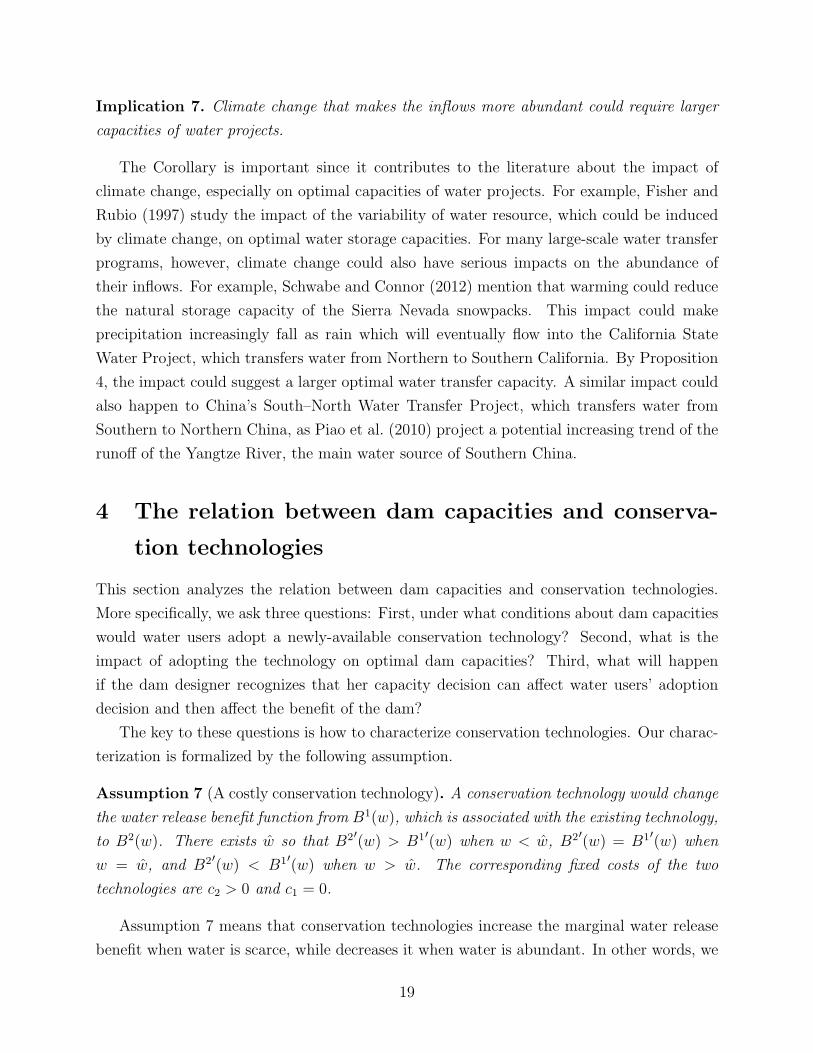
Assumption 7 (A costly conservation technology). A conservation technology would change

the water release benefit function from B1(w), which is associated with the existing technology,

to B2(w). There exists w so that B2′(w) > B1′(w) when w < w, B2′(w) = B1′(w) when

w = w, and B2′(w) < B1′(w) when w > w. The corresponding fixed costs of the two

technologies are c2 > 0 and c1 = 0.

Assumption 7 means that conservation technologies increase the marginal water release

benefit when water is scarce, while decreases it when water is abundant. In other words, we

19

assume that conservation technologies rotate clockwise the marginal water release benefit

function. Notably, this characterization is different to that in Zhao and Zilberman (2001) for

example, in which the conservation technology shifts down the marginal benefit of resource,

but consistent with that in Caswell and Zilberman (1986) and some other literature.

Assumption 7 is straightforward, if we assume 1) that the water release benefit equals

to a benefit function in effective water, whose share in the released water is increased by

conservation technologies, 2) that there is a finite upper bound of the water release benefit,

which could result from some constraints on the expansion of the water using sector, and

3) that the curvature of the marginal effective water benefit isn’t too positive. As argued

in Caswell and Zilberman (1986), the Assumption means that the elasticity of the marginal

effective water benefit with respect to effective water crosses one, which is more plausible in

irrigation water use, than some other specifications of the effective water benefit function,

for example the Cobb and Douglas (1928) specification, are. We show the following example

to illustrate the Assumption. A more formal justification can be found in Appendix B.

Example 1 Consider an effective water benefit function B(W) = W(2a−W), where W ∈[0, a] is the effective water, and a > 0 is a parameter. Note that the effective water benefit

function is weakly increasing, and that its marginal value is weakly decreasing. Assume a

technology is assumed to effectively use α of the water release, w, so W = αw. Therefore

we can write the water release benefit function as B(w) = αw(2a − αw). The marginal

water release benefit is then B′(w) = 2aα − 2α2w. Now consider the existing technology

that gives α = α1 and the conservation technology that gives α = α2, where α2 > α1. The

two corresponding marginal water release benefit functions are then respectively B1′(w) =

2aα1 − 2α21w and B2′(w) = 2aα2 − 2α2

2w. Since α2 > α1, the intercept on the vertical

axis of B2′(w) is then higher than B1′(w)’s, the intercept on the horizontal axis of B2′(w)

is then lower than B1′(w)’s, and B2′(w) is steeper than B1′(w). Simple algebra also gives

w = aα2+α1

. We can conclude that the conservation technology rotates clockwise the marginal

water release benefit function around w = w.

Under Assumption 7, we answer the three important questions in the following Subsec-

tions, respectively.

4.1 Impacts of dam capacities on conservation technology adop-

tion

Under what conditions about dam capacities would water users adopt a newly-available

conservation technology? To answer this question, first assume the representative potential

20

adopter is rational.

Assumption 8 (Rational adoption of the representative water user). The representative

water user chooses whether to switch from the existing technology to the conservation tech-

nology by comparing the respective discounted expected sums of water release benefits net of

the fixed costs.

Assumption 8 implies that the conservation technology will be adopted if and only if the

representative water user could gain from the adoption. Mathematically, under Assumptions

1, 2, 4, 5, 7, and 8, the representative water user’s technology adoption problem is

maxi∈{1,2}

E0

[∞∑s=0

ρsBis(min {es, w})

]− ci, (8)

which is equivalent to

maxi∈{1,2}

1

1− ρ

[∫ w

−∞Bi(e)f(e)de+ (1− F (w))Bi(w)

]− ci, (9)

and the water user will adopt the conservation technology, which means i∗ = 2, if and only

if ∫ w

−∞ (B2(e)−B1(e)) f(e)de+ (1− F (w)) (B2(w)−B1(w))

1− ρ> c2. (10)

The left-hand side of the condition is the discounted comparative benefit of adopting the

conservation technology over not adopting, or the conservation technology’s advantage, and

the right-hand side is the fixed cost of the adoption. For notational simplicity, denote the

left-hand side as A(w), where A represents advantage. To investigate its shape, we calculate

its derivative and have

A′(w) =1

1− ρ(1− F (w))

(B2′(w)−B1′(w)

), (11)

which means

A′(w) > 0 and A(w) is increasing, if w < w;

A′(w) = 0 and A(w) reaches its maximum, if w = w;

A′(w) < 0 and A(w) is decreasing, if w > w. (12)

This analysis implies that the conservation technology’s advantage is smaller with large or

small dams than with dams of moderate capacities. This implication proves the following

Proposition, which documents the impact of dam capacities on conservation technology

21

adoption.

Proposition 5 (Too small or too large dams discourage adopting conservation technologies).

Under Assumptions 1, 2, 4, 5, 7, and 8, if the dam is too large or too small, then the

conservation technology won’t be adopted. Mathematically and more precisely, the following

two statements are true:

1) If A(w) > c2, then the conservation technology will be adopted if and only if ws < w <

wl, where ws and wl solve A(w) = c2.

2) If A(w) ≤ c2, then given any w, the conservation technology won’t be adopted.

Figure 6 illustrates the first statement in Proposition 5. The top panel exhibits that the

conservation technology rotates clockwise the marginal water release benefit function around

w = w. The mid panel presents the marginal advantage of the conservation technology, which

intersects the horizontal axis from above at w = w. The bottom panel shows the advantage,

which flips its monotonicity in w at w = w. In the panel, a horizontal line of height c2

intersects A(w), and identifies the two roots to A(w) = c2, ws and wl. The three panels give

the following observations: when the dam is small, the conservation technology is marginally

more beneficial than the existing technology, but the cumulative benefit isn’t large enough to

cover the fixed cost of adoption; when the dam is large, then the conservation technology is

marginally less beneficial than the existing technology, so the cumulative benefit is decreasing

and the fixed cost becomes even more difficult to be covered; only when the dam is neither

too small nor too large, the conservation technology will be sufficiently more beneficial than

the existing technology to cover the fixed cost, and it will then be adopted.

From the bottom panel of Figure 6, it is also clear that A(w) won’t reach the horizon-

tal line of height c2 when c2 is sufficiently large, which is about the second statement in

Proposition 5.

To my knowledge, Proposition 5 is the first result about impacts of public water projects

on conservation technology adoption, though public water projects usually affect a large

number of water users and potential adopters. Following the threshold model of technol-

ogy adoption in David (1975), numerous theoretical and empirical studies about irrigation

and conservation technology adoption have emerged. Caswell (1991) surveys the literature

about factors affecting adoption choices. Notable examples include Feinerman (1983), Fein-

erman and Vaux (1984), Caswell and Zilberman (1986), Dinar and Knapp (1986), Caswell

et al. (1990), Dinar and Yaron (1990, 1992), Dinar and Letey (1991), Dinar and Zilberman

(1991a,b), Dinar et al. (1992), Lynne et al. (1995), Shah et al. (1995), Green et al. (1996),

Khanna and Zilberman (1997), Carey and Zilberman (2002), Foltz (2003), and Koundouri

et al. (2006), among others. The factors in focus include farm size, labor availability, tenure

22

Figure 6: Impacts of dam capacities on conservation technology adoption

systems, market imperfection and learning cost, economic variables (water price and oth-

ers), capital constraints, water-related endowments (land quality, well depth, climate, and

others), production risk, human capital, resource exhaustibility, water markets, agricultural

characteristics, policies, and psychology, among others, and good surveys are also written by

Feder et al. (1985), Sunding and Zilberman (2001), and Schoengold and Zilberman (2007).

Apparently no studies, however, have ever discussed the impact of dam capacities.14 Propo-

14One reason for the lack of attention of the impact of water projects on conservation technology adoption

23

sition 5 fills the gap by showing a non-monotonic impact of dam capacities on the incentive

of adopting conservation technologies.

Proposition 5 is also consistent with the studies on the potential non-monotonic relation

between resource abundance and conservation technology adoption. Caswell and Zilberman

(1986) shows that when applied water is little, adopting conservation technologies could

induce more water usage, while the opposite could happen when applied water is already a

lot, since the elasticity of the marginal product with respect to the effectively applied water

could cross unity when the applied water increases. This theoretical result is well recognized

in many papers (e.g. Caswell et al. (1990), Dinar et al. (1992), Dinar and Zilberman (1991a),

Shah et al. (1995), Dridi and Khanna (2005), Lichtenberg (2013), and Lin (2014)) and surveys

(e.g. Feder and Umali (1993) and Lichtenberg (2002)). The non-monotonicity, especially the

increasing part, has also been shown empirically relevant by studies like Peterson and Ding

(2005), Frisvold and Emerick (2008), and Lin (2014), among others.15 Proposition 5 shows

that this potential non-monotonic relation could be applicable to water project capacities.

Proposition 5 suggests that governments can encourage conservation technology adoption

by building larger dams or closing some water projects. To find the correct policy, the

governments should have good knowledge about the reason why people don’t adopt the

technology: Is water so abundant that there is no need to conserve, or so scarce that there

is little aggregate gain from conservation? This is an empirical question that should be

answered seriously.

4.2 Impacts of conservation technologies on optimal dam capaci-

ties

Will water users’ adoption of conservation technologies require larger or smaller dams? Since

conservation technologies change the water release benefit function, the following Proposition

answers the question by comparative static analysis of our capacity determination model

around the water release benefit.

Proposition 6 (Conservation technologies require smaller dams if and only if the dams are

already large). Under Assumptions 1, 2, 3, 4, 5, and 6, and 7, if the initial optimal dam

capacity is small, then adopting the conservation technology requires a larger optimal dam

could be the difficulty in empirically identifying the impact: on the one hand, as public water projects affecta large number of water users, there is little variation in the water project capacity across these water users;on the other hand, across the water users with different water projects, it is also difficult to argue that thereare few confounding factors when we attempt to estimate the impact of water project capacity.

15Another non-monotonic relation is presented by Carey and Zilberman (2002), in which the impact ofwater markets on adoption has an opposite interactions with water endowment in the case of water abundanceto the case of water scarcity.

24

capacity; if the initial optimal dam capacity is large, then adopting the conservation technol-

ogy requires a smaller optimal dam capacity. Mathematically and more precisely, consider

the optimal dam capacities with the existing technology and the conservation technology, w∗1

and w∗2. If w∗1 < w, then w∗1 < w∗2 < w; if w∗1 = w, then w∗1 = w∗2 = w; if w∗1 > w,

then w < w∗2 < w∗1.

Figure 7 illustrates Proposition 6. Since adopting the conservation technology rotates

clockwise the marginal water release benefit function, whether it rotates up or down the

marginal benefit of dam capacities depends on whether the marginal benefit intersects the

marginal cost on the left or on the right of w: if the initial dam capacity is small, then

adopting the conservation technology rotates up the marginal benefit of dam capacities.

Following the logic in Proposition 2, the optimal dam capacity increases. If the initial dam

capacity is large, then a similar but opposite logic holds.

Figure 7: Impacts of conservation technologies on optimal dam capacities

Compared with literature about capacity determination, including Tsur (1990), Fisher

and Rubio (1997), Schoengold and Zilberman (2007, p.2943,2955), and others, it is a novel

contribution that Proposition 6 identifies conservation technology adoption as a potential

factor affecting the dam capacity decision. Proposition 6 also contrasts the cost-minimization

logic mentioned in Section 3. We prove in Appendix C that given any capacity, the dam

with the conservation technology can generate more benefit than that with the existing

25

technology does. Along the cost-minimization logic and with the target benefit level being

the benefit of the dam with the existing technology, the best decision of dam capacity would

then be unambiguously smaller than the initial dam capacity with the existing technology.

The social optimal dam capacity with the conservation technology, however, would depend

on the critical capacity level w, and is larger than the initial dam capacity when the initial

optimal dam capacity is small.

4.3 Impacts of potential adoption of conservation technologies on

optimal dam capacities

Proposition 6 assumes that adopting conservation technologies is given. An even more

interesting situation is where the water users can choose whether to adopt the conservation

technology at the fixed cost after the social planner has decided the dam capacity. In other

words, the dam designer should recognize that her capacity decision will affect water users’

adoption decision, and then affect the benefit of the dam. What is the impact of the potential

adoption on the dam capacity problem?16

First we formalize the situation by the following Assumption.

Assumption 9 (Potential adoption of conservation technologies). A(w) > c2, and the social

planner acknowledges the potential costly adoption of the conservation technology.

Assumption 9 means first, that there exists a range of capacities that can induce adoption

of the conservation technology, and second, that the dam designer is a von Stackelberg

leader and the representative water user is the follower. Similar problems have been seen

in Zhao and Zilberman (2001), for example, in a case about resource restoration. Different

to their focus on the option value and optimal timing of resource development, the von

Stackelberg setting of our analysis, as we shall show now, makes the potential adoption

create a discontinuous marginal benefit of dam capacities.

Recall that the marginal benefit of dam capacities is

1

1− ρ(1− F (w))B′(w) +

1

1− ρ

∫ ∞

w

L′(e− w)f(e)de. (13)

Therefore, when the dam capacity does or doesn’t lie in the range that induces the adoption,

the marginal benefit of dam capacities is calculated with different marginal water release

16The question can be generalized into a classic economic question about the interaction between a regu-lator and the regulated. For example, Amacher and Malik (2002) analyze the properties of a pollution taxwhen the regulated firms chooses abatement technologies. For more detail about the literature, see Amacherand Malik (2002)’s references.

26

benefit functions. The marginal benefit should then experience discontinuity when the dam

capacity moves into or out of the range. Mathematically, under Assumptions 1, 2, 3, 4, 5,

6, 7, 8, and 9, the marginal benefit of dam capacities turns out to be

1

1− ρ(1− F (w))B1′(w) +

1

1− ρ

∫ ∞

w

L′(e− w)f(e)de, if w ≤ ws or w ≥ wl;

1

1− ρ(1− F (w))B2′(w) +

1

1− ρ

∫ ∞

w

L′(e− w)f(e)de, if ws < w < wl. (14)

The discontinuity suggests multiple intersections between the marginal benefit of dam capac-

ities and the marginal cost, and therefore multiple solutions to Equation (5), the first-order

condition. This observation is documented by the following Proposition.

Proposition 7 (Multiple solutions with potential adoption of conservation technologies).

Under Assumptions 1, 2, 3, 4, 5, 6, 7, 8, and 9, it is possible to have multiple solutions to

Equation 5, the first-order condition of the capacity determination problem.

Figure 8 illustrates Proposition 7. In the Figure, the marginal benefit of dam capacities

is shown by the solid lines, and it is clear that the marginal benefit experiences discontinuity

at the boundaries of the range that induces adoption, ws and wl. We circled all intersections

in all possible cases of the marginal cost function. The two interesting cases that induces

multiple intersections are also circled by dotted lines. We address them in the following two

Cases, respectively.

Case 1 Figure 9 illustrates this case. In this case, there are two intersections, w∗2 and

w∗1, corresponding to adopting the conservation technology and not adopting it. Moreover,

w∗1 < ws < w∗2 < w.

The social planner then faces the ultimate choice: a small dam with neither adoption nor

the fixed cost, versus a not large dam with adoption and the fixed adoption cost. In Figure

9, the key to the choice is the comparison between the shadowed areas. To see this point,

note 1) that without adoption, the increase in social welfare when the capacity moves from

ws to w∗1 equals to the size of the lower shadowed area, 2) that with adoption, the increase

in social welfare when the capacity moves from ws to w∗2 equals to the size of the higher

shadowed area, and 3) that when the capacity is ws, the social welfare with adoption and

that without adoption are the same.17 Therefore, if the higher shadowed area is larger, then

the capacity that induces adoption, w∗2, implies higher social welfare than w∗1 does. As the

17To see the third point, note when the capacity is ws, the water release benefits including fixed costs ofthe technologies are the same.

27

Figure 8: Impacts of potential adoption of conservation technologies on optimal damcapacities

Figure 9: Impacts of potential adoption of conservation technologies on optimal damcapacities: Multiple intersections when dams are small

comparison depends on the steepness of the marginal cost of dam capacities, we have the

following Corollary.

Corollary 1. In Case 1, under Assumptions 1, 2, 3, 4, 5, 6, 7, 8, and 9, if the marginal

cost of dam capacities is increasing slowly, then the optimal dam capacity induces adoption.

28

Mathematically and more precisely, if C ′′(·) +D′′(·) is small, then w∗ = w∗2.

Case 2 Figure 10 illustrates this case. In this case, there are two intersections, w∗2 and

w∗1, corresponding to adopting the conservation technology and not adopting it. Moreover,

w < w∗2 < wl < w∗1.

Figure 10: Impacts of potential adoption of conservation technologies on optimal damcapacities: Multiple intersections when dams are large

The social planner then face the ultimate choice: a large dam with adoption and the

fixed cost, versus a not small dam with neither adoption nor the fixed cost. Along a similar

logic to that in Case 1, we have the following Corollary.

Corollary 2. In Case 2, under Assumptions 1, 2, 3, 4, 5, 6, 7, 8, and 9, if the marginal cost

of the dam capacity is increasing fast and the existing technology is very weak with abundant

water, then the optimal dam capacity induces adoption. Mathematically and more precisely,

if C ′′(·) +D′′(·) is large, then w∗ = w∗2.

Case 2 also sheds some new light on the logic of oversized water projects. Schoengold and

Zilberman (2007) show that oversized water projects could be resulted from the distortion

in the marginal dam cost. Our analysis suggests that they could also be induced by the dam

designer’s overlooking of the potential future adoption of conservation technologies.

Compared with our analysis in the former Subsection, the two Cases imply that the

impacts of potential adoption on optimal dam capacities are more complicated than the case

29

with given adoption. This complication asks for serious empirical analysis about the impact

of conservation technologies on the marginal water release benefit, since the analysis would

help to identify the critical capacity levels, ws and wl, and whether the marginal cost of dam

capacities is steep enough.

5 Conclusion

This paper develops a stylized model for the determination of optimal dam capacities, and

analyzes how it varies under plausible scenarios. Comparative static analysis of the models

shows the impact of water management efficiency, overflow losses, and climate change on

optimal water project capacities: integrated water reforms, emphasis on food security, and

warming-caused inflow abundance could make larger water projects desirable. This paper

also systematically analyzes the non-monotonic relation between dam capacities and conser-

vation technologies, probably as the first attempt in literature: too small or too large wa-

ter projects could discourage conservation technology adoption, adoption suggests smaller

projects if and only if the projects are already large, and one reason for oversized water

projects could be the designer’s overlooking of the future potential adoption of conservation

technologies.

The model and analysis in this paper can be extended to several nontrivial directions. For

example, further effort can assume water users heterogenous, and model a non-monotonic

impact of dam capacities on the percentage of adoption in a population of water users. A

water distribution system can be added, and it is natural to expect that only the water

users neither too close to nor too far away from the water source would adopt conservation

technologies. Results that are parallel to the Propositions can be derived if we incorporate

optimal water-inventory control, as we are doing in Xie and Zilberman (2014). Moreover,

this paper asks for more serious empirical tests on the derived analytical results.

To conclude, our paper provides a new analytical framework, suggesting that the design

of water projects is not divorced from the efficiency of water use downstream, and that the

changes in the institutional, environmental, and technological conditions could significantly

modify the optimal scale of water projects. The issue is not how large is a water project but

how valuable are the water economic and environmental services that the project provides.

The framework can serve as a starting point for investigation in future research, on the

economics and policy implications about the design and improvements of water systems.

30

References

102nd United States Congress. 1992. Central Valley Project Improvement Act (Public Law 102-575,Title 34). Washington, Disctrict of Columbia: United States Congress.

Amacher GS, Malik AS. 2002. Pollution taxes when firms choose technologies. Southern EconomicJournal 68: 891–906.

Arrow KJ, Fisher AC. 1974. Environmental preservation, uncertainty, and irreversibility. QuarterlyJournal of Economics 88: 312–319.

Brill E, Hochman E, Zilberman D. 1997. Allocation and pricing at the water district level. AmericanJournal of Agricultural Economics 79: 952–963.

Burness HS, Quirk JP. 1979. Appropriative water rights and the efficient allocation of resources.American Economic Review 69: 25–37.

Burt OR. 1964. Optimal resource use over time with an application to ground water. ManagementScience 11: 80–93.

Burt OR. 1966. Economic control of groundwater reserves. Journal of Farm Economics 48: 632–647.

Burt OR. 1967. Temporal allocation of groundwater. Water Resources Research 3: 45–56.

Burt OR. 1970. Groundwater storage control under institutional restrictions. Water ResourcesResearch 6: 1540–1548.

Calefati J. 2014. California drought: So many water bonds, so little time. San Jose Mercury News,March 22, 2014.

Carey JM, Zilberman D. 2002. A model of investment under uncertainty: Modern irrigationtechnology and emerging markets in water. American Journal of Agricultural Economics 84:171–183.

Carvalho E. 2014. Transpor agua do Rio Paraıa do Sul nao resolve problema de SP, diz ONG. G1,March 19, 2014.

Caswell MF. 1991. Irrigation technology adoption decisions: Empirical evidence. In Dinar A,Zilberman D (eds.) The Economics and Management of Water and Drainage in Agriculture.New York: Springer Verlag, 295–312.

Caswell MF, Lichtenberg E, Zilberman D. 1990. The effects of pricing policies on water conservationand drainage. American Journal of Agricultural Economics 72: 883–890.

Caswell MF, Zilberman D. 1986. The effects of well depth and land quality on the choice of irrigationtechnology. American Journal of Agricultural Economics 68: 798–811.

Chakravorty U, Hochman E, Umetsu C, Zilberman D. 2009. Water allocation under distributionlosses: Comparing alternative institutions. Journal of Economic Dynamics and Control 33:463–476.

31

Chakravorty U, Hochman E, Zilberman D. 1995. A spatial model of optimal water conveyance.Journal of Environmental Economics and Management 29: 25–41.

Chatterjee B, Howitt RE, Sexton RJ. 1998. The optimal joint provision of water for irrigation andhydropower. Journal of Environmental Economics and Management 36: 295–313.

Cheng W. 2014. The second navigation lock of the Three Gorges Dam discussed by Ministriesand Commissions (Duo Buwei yi diaoyan toujian Sanxia Daba di’er chuanzha). 21st CenturyBusiness Herald (21 Shiji Jingji Baodao), April 30, 2014.

Chong H, Sunding D. 2006. Water markets and trading. Annual Review of Environment andResources 36: 239–264.

Cobb CW, Douglas PH. 1928. A theory of production. American Economic Review 18: 139–165.

Congressional Budget Office of the United States. 1997. Water Use Conflicts in the West: Implica-tions of Reforming the Bureau of Reclamation’s Water Supply Policies. Washington, the Districtof Columbia: Congress of the United States.

David PA. 1975. Technical Choice Innovation and Economic Growth: Essays on American andBritish Experience in the Nineteenth Century. London: Cambridge University Press.

de Arauo T. 2014a. Crise da agua em SP: Voce ja bebeu “volume morto”? Em breve ele chegaraa sua casa. Brasil Post, April 11, 2014.

de Arauo T. 2014b. Entenda a guerra da agua entre Sao Paulo e Rio de Janeiro. Brasil Post, March21, 2014.

Dinar A, Campbell MB, Zilberman D. 1992. Adoption of improved irrigation and drainage reductiontechnologies under limiting environmental conditions. Environmental and Resource Economics2: 373–398.

Dinar A, Knapp KC. 1986. A dynamic analysis of optimal water use under saline conditions.Western Journal of Agricultural Economics 11: 58–66.

Dinar A, Letey J. 1991. Agricultural water marketing, allocative efficiency, and drainage reduction.Journal of Environmental Economics and Management 20: 210–223.

Dinar A, Tsur Y. 1995. Efficiency and equity considerations in pricing and allocating irrigationwater. World Bank Policy Research Working Paper No. 1460.

Dinar A, Yaron D. 1990. Influence of quality and scarcity of inputs on the adoption of modernirrigation technologies. Western Journal of Agricultural Economics 14: 224–233.

Dinar A, Yaron D. 1992. Adoption and abandonment of irrigation technologies. AgriculturalEconomics 6: 315–332.

Dinar A, Zilberman D. 1991a. The economics of resource-conservation, pollution-reduction tech-nology selection: The case of irrigation water. Resources and Energy 13: 323–348.

Dinar A, Zilberman D. 1991b. Effects of input quality and environmental conditions on selectionof irrigation technologies. In Dinar A, Zilberman D (eds.) The Economics and Management ofWater and Drainage in Agriculture. New York: Springer US, 229–250.

32

Dridi C, Khanna M. 2005. Irrigation technology adoption and gains from water trading underasymmetric information. American Journal of Agricultural Economics 87: 289–301.

Duflo E, Pande R. 2007. Dams. Quarterly Journal of Economics 122: 601–646.

Feder G, Just RE, Zilberman D. 1985. Adoption of agricultural innovations in developing countries:A survey. Economic Development and Cultural Change 33: 255–298.

Feder G, Umali DL. 1993. The adoption of agricultural innovations: A review. TechnologicalForecasting and Social Change 43: 215–239.

Feinerman E. 1983. Crop density and irrigation with saline water. Western Journal of AgriculturalEconomics 8: 134–140.

Feinerman E, Vaux HJ Jr. 1984. Uncertainty and the management of salinity with irrigation water.Western Journal of Agricultural Economics 9: 259–270.

Feinstein D. 2014a. California, Oregon Senators introduce drought relief legislation. Dianne Fein-stein Press Releases, Feburary 11, 2014.

Feinstein D. 2014b. Feinstein, Boxer preparing California drought legislation. Dianne FeinsteinPress Releases, Feburary 5, 2014.

Fischhendler I, Zilberman D. 2005. Packaging policies to reform the water sector: The case of theCentral Valley Project Improvement Act. Water Resources Research 41.

Fisher AC, Rubio SJ. 1997. Adjusting to climate change: Implications of increased variabilityand asymmetric adjustment costs for investment in water reserves. Journal of EnvironmentalEconomics and Management 34: 207–227.

Foltz JD. 2003. The economics of water-conserving technology adoption in Tunisia: An empiricalestimation of farmer technology choice. Economic Development and Cultural Change 51: 359–373.

Freking K. 2014. Congress focuses on dams amid California’s drought. Associated Press, March23, 2014.

Frisvold GB, Emerick KJ. 2008. Rural-urban water transfers with applications to the U.S. Mexicoborder region. In Dinar A, Albiac J, Sanchez-Soriano J (eds.) Game Theory and Policy Makingin Natural Resources and the Environment. New York: Routledge Press.

Garamendi J. 2014a. Congressmen Garamendi and LaMalfa announce Sites Reservoir Water Stor-age Bill. John Garamendi Press Releases, March 19, 2014.

Garamendi J. 2014b. A water plan for all of California. John Garamendi Press Releases, March27, 2014.

Gisser M, Johnson RN. 1984. Institutional restrictions on the transfer of water rights and the sur-vival of an agency. In Anderson TL (ed.) Water Rights: Scarce Resource Allocation, Bureaucracy,and the Environment. New York: Harper & Row Publishers.

Gisser M, Sanchez DA. 1980. Competition versus optimal control in groundwater pumping. WaterResources Research 16: 638–642.

33

Green CH, Parker DJ, Tunstall SM. 2000. Assessment of flood control and management options. InSecretariat of the World Commission on Dams (ed.) Options Assessment: IV.4, WCD ThematicReview. Cape Town: World Commission on Dams.

Green G, Sunding D, Zilberman D, Parker DD. 1996. Explaining irrigation technology choices: Amicroparameter approach. American Journal of Agricultural Economics 78: 1064–1072.

Howe CW, Schurmeier DR, Shaw WD Jr. 1986. Innovative approaches to water allocation: Thepotential for water markets. Water Resources Research 22: 439–445.

Jackson S, Sleigh A. 2000. Resettlement for China’s Three Gorges Dam: Socio-economic impactand institutional tensions. Communist and Post-Communist Studies 33: 223–241.

Kennedy B. 2001. China’s Three Gorges Dam. Cable News Network.

Khanna M, Zilberman D. 1997. Incentives, precision technology and environmental protection.Ecological Economics 23: 25–43.

Koundouri P, Nauges C, Tzouvelekas V. 2006. Technology adoption under production uncertainty:Theory and application to irrigation technology. American Journal of Agricultural Economics88: 657–670.

Lichtenberg E. 2002. Agriculture and the environment. Handbook of Agricultural Economics 2:1249–1313.

Lichtenberg E. 2013. Optimal investment in precision irrigation systems: A dynamic intraseasonalapproach. 2013 Agricultural and Applied Economics Association and Canadian AgriculturalEconomics Society Joint Annual Meeting, August 2013.

Lin LPCYC. 2014. Does efficient irrigation technology lead to reduced groundwater extraction?Empirical evidence. Journal of Environmental Economics and Management 67: 189–208.

Lynne GD, Casey CF, Hodges A, Rahmani M. 1995. Conservation technology adoption decisionsand the theory of planned behavior. Journal of Economic Psychology 16: 581–598.

Lyons C. 2012. The dam boom in the Amazon. The New York Times, June 30, 2012.

McCully P. 2001. Silenced Rivers: The Ecology and Politics of Large Dams. London: Zed Books.

Nirappil F. 2014. Two Northern California congressmen seek momentum to build new reservoir.Associated Press, March 20, 2014.

Peterson JM, Ding Y. 2005. Economic adjustments to groundwater depletion in the High Plains:Do water-saving irrigation systems save water? American Journal of Agricultural Economics87: 147–159.

Piao S, Ciais P, Huang Y, Shen Z, Peng S, Li J, Zhou L, Liu H, Ma Y, Ding Y, Friedlingstein P,Liu C, Tan K, Yu Y, Zhang T, Fang J. 2010. The impacts of climate change on water resourcesand agriculture in China. Nature 467: 43–51.

Quiggin J. 2006. Repurchase of renewal rights: A policy option for the National Water Initiative.Australian Journal of Agricultural and Resource Economics 50: 425–435.

34

Saleth RM, Dinar A. 2000. Institutional changes in global water sector: Trends, patterns, andimplications. Water Policy 2: 175–199.

Schoengold K, Sproul T, Zilberman D. 2008. Irrigated agriculture in an era of high energy prices.In Villacampa Esteve Y, Brebbia CA, Prats Rico D (eds.) Sustainable irrigation: Management,technologies and policies II, volume 112 of WIT Transactions on Ecology and the Environment.Southampton: WIT Press.

Schoengold K, Zilberman D. 2007. The economics of water, irrigation, and development. Handbookof Agricultural Economics 3: 2933–2977.

Schwabe KA, Connor JD. 2012. Drought issues in semi-arid and arid environments. Choices 27.

Shah FA, Zilberman D, Chakravorty U. 1995. Technology adoption in the presence of an exhaustibleresource: The case of groundwater extraction. American Journal of Agricultural Economics 77:291–299.

Simonovic SP. 1992. Reservoir systems analysis: Closing gap between theory and practice. Journalof Water Resources Planning and Management 118: 262–280.

Singh S. 2002. Taming the Waters: The Political Economy of Large Dams in India. New Delhi:Oxford University Press.

Sunding D, Zilberman D. 2001. The agricultural innovation process: Research and technologyadoption in a changing agricultural sector. Handbook of Agricultural Economics 1: 207–261.

The Economist. 2013a. Opening the floodgates. The Economist, September 21, 2013.

The Economist. 2013b. The rights and wrongs of Belo Monte. The Economist, May 4, 2013.

Truong CH. 2012. An analysis of storage capacity reallocation impacts on the irrigation sector.Environmental and Resource Economics 51: 141–159.

Tsur Y. 1990. The stabilization role of groundwater when surface water supplies are uncertain:The implications for groundwater development. Water Resources Research 26: 811–818.

Tsur Y. 2009. On the economics of water allocation and pricing. Annual Review of ResourceEconomics 1: 513–536.

Tsur Y, Graham-Tomasi T. 1991. The buffer value of groundwater with stochastic surface watersupplies. Journal of Environmental Economics and Management 21: 201–224.

United States Department of Interior, United States Bureau of Reclamation, United States Fishand Wildlife Service. 1999. Central Valley Project Improvement Act Final Programmatic Envi-ronmental Impact Statement: Executive Summary. Sacramento, California.

United States Water Resources Council. 1983. Economic and environmental principles and guide-lines for water and related land resources implementation studies. Washington, the District ofColumbia: United States Government Printing Office.

von Stackelberg HF. 1934. Marktform und Gleichgewicht. Vienna: Julius Springer.

35

Wittfogel KA. 1957. Oriental Despotism: A Comparative Study of Total Power. London: OxfordUniversity Press.

Xie Y, Zilberman D. 2014. The economics of water project capacities under optimal water in-ventory management. Uncompressed working paper, Department of Agricultural and ResourceEconomics, University of California, Berkeley.

Yeh WWG. 1985. Reservoir management and operations models: A state-of-the-art review. WaterResources Research 21: 1797–1818.

Zhao J, Zilberman D. 1999. Irreversibility and restoration in natural resource development. OxfordEconomic Papers 51: 559–573.

Zhao J, Zilberman D. 2001. Fixed costs, efficient resource management, and conservation. AmericanJournal of Agricultural Economics 83: 942–957.

Zilberman D, Griffin RC, Parker DD, Mazzotta MJ, Opaluch JJ, Hyde WF, Larson DM, FisherAC. 1994. Review of Principles and Guidelines. Berkeley, California: Department of Agriculturaland Resource Economics, University of California.

Zilberman D, Schoengold K. 2005. The use of pricing and markets for water allocation. CanadianWater Resources Journal 30: 47–54.

A Appendix: Cheaper cost, larger dams

Innovation in construction and maintenance cost efficiency or decrease in the marginal environmen-tal damage can also affect optimal dam capacities.

Proposition 8 (Cheaper or more environmentally-friendly dam-building technologies encourageslarger dams). Under Assumptions 1, 2, 3, 4, 5, and 6, if improvement in dam construction andmaintenance cost efficiency shifts down the marginal construction and maintenance cost of damcapacities, or more environmentally-friendly dam building technologies shifts down the marginalenvironmental damage cost of dam capacities, then the optimal dam capacity becomes larger. Mathe-matically, consider two functions of the construction and maintenance cost of dam capacities, C1(·)and C2(·), two functions of the environmental damage cost of dam capacities, D1(·) and D2(·), andthe two corresponding optimal dam capacities, w∗1 and w∗2. If C2′(·) ≤ C1′(·) or D2′(·) ≤ D1′(·),then w∗2 ≥ w∗1.

B Appendix: Justification of Assumption 7

Assumption 7 reads:

There exists w so that B2′(w) > B1′(w) when w < w, B2′(w) = B1′(w) whenw = w, and B2′(w) < B1′(w) when w > w.

To justify this Assumption, consider an effective water benefit function B(W), where W is theeffective water. Assume B(·) is smooth, −∞ < B(∞) < ∞, 0 < B′(0) < ∞, B′′(·) < 0, and B′′′(·)

36

is not large so that B′′′(x) < −2B′′(x)/x for x ∈ (0,∞). A technology is assumed to use α of waterrelease w effectively.

The water release benefit function is then B(w,α) ≡ B(αw). The marginal benefit of water

release is then ∂B(w,α)∂w ≡ αB′(αw). Now consider the impact of α on ∂B(w,α)

∂w . The partial derivative

of ∂B(w,α)∂w with respect to α is

∂2B(w,α)

∂α∂w= B′(αw) + αwB′′(αw). (15)

On the one hand, since 0 < B′(0) < ∞, ∂2B(w,α)∂α∂w |w=0

= B′(0) ∈ (0,∞). Since B(·) is smooth,

there must exist w > 0 such that∫ w0

∂2B(w,α)∂w∂α dw > 0.

On the other hand, since B(∞, α) = B(∞) ∈ (−∞,∞),

∂B(w,α)

∂α |w=∞= 0,∫ ∞

0

∂2B(w,α)

∂w∂αdw = 0,

(16)

Therefore,∫∞w

∂2B(w,α)∂w∂α dw < 0, which means there must exist w > 0 such that ∂2B(w,α)

∂w∂α |w=w< 0.

As ∂2B(w,α)∂α∂w |w=0

= B′(0) > 0, ∂2B(w,α)∂w∂α |w=w

< 0, and ∂2B(w,α)∂w∂α is continuous, there must exist w

such that ∂2B(w,α)∂w∂α |w=w

= 0.

The partial derivative of ∂2B(w,α)∂w∂α with respect to w is

∂3B(w,α)

∂w2∂α= 2αB′′(αw) + α2wB′′′(αw). (17)

Since B′′′(x) < −2B′′(x)/x, ∂3B(w,α)∂w2∂α

< 0, which means ∂2B(w,α)∂w∂α is decreasing in w. Therefore, the

impact of α on ∂B(w,α)∂w is

∂2B(w,α)

∂α∂w> 0, if 0 < w < w;

∂2B(w,α)

∂α∂w= 0, if w = w;

∂2B(w,α)

∂α∂w< 0, if w > w.

(18)

There are two technologies: the existing one can use α1 of water release w effectively, and thenewly available conservation technology can use α2 of water release w effectively, where α2 > α1.The corresponding water release benefit functions are respectively B1(w) ≡ B(α1w) and B2(w) ≡B(α2w). Assumption 7 then follows the impact of α on ∂B(w,α)

∂w .

37

C Appendix: Dams are more valuable with the con-

servation technology than those with the existing

technology

Following the analysis in Appendix B, the dam with the conservation technology always generatesmore benefit than the dam of the same capacity but with the existing technology. To see this point,note the dam of capacity w can generate the benefit of∫ w

0

1

1− ρ(1− F (x))αB′(αx)dx

=

∫ w

0

1

1− ρ(1− F (x))B′(αx)d(αx)

=

∫ w

0

1

1− ρ(1− F (x))dB(αx)

=1

1− ρ

[(1− F (w))B(αw)−

∫ w

0B(αx)d(1− F (x))

]=

1

1− ρ

[(1− F (w))B(αw) +

∫ w

0B(αx)dF (x)

].

(19)

Assume B′(·) ≥ 0 for all x ≥ 0. The benefit is then increasing in α, which means given anycapacity, dams are more valuable with the conservation technology than those with the existingtechnology.

D Appendix: The marginal water release benefit is

shifted up by the transition from water rights to

water markets

Assume the water release w is supplied to an agricultural area by an utility with a supply costfunction SC(w), which satisfies SC(0) > 0, SC ′(·) > 0, and SC ′′(·) > 0. Assume that before thetransition from water rights to water markets, the irrigation demand or marginal benefit of wateruse in agriculture is AB1

′(w), and the water is priced as the average supply cost, SC(w)w . Assume

that after the transition, the irrigation demand is AB2′(w), and the water is priced as the marginal

supply cost, SC ′(w). Assume ABi′(·) > 0 and ABi

′′(·) < 0, where i = 1, 2.It is easy to calculate the marginal water release benefit Bi′(w) as ABi

′(w)−SC ′(w)+NAB′(w),where i = 1, 2, and NAB′(w) is the marginal water release benefit not from irrigation, guaranteeingnonnegative Bi′(·), which is required by Assumption 2.

The transition includes the high willingness-to-pay of the highly efficient individuals for addi-tional water into the marginal water-use benefit, so AB2

′(·) > AB1′(·).

The transition also has water priced by the marginal cost instead of the average cost. Forexample, we assume that the water release w will be supplied if and only if it isn’t larger than theequilibrium quantity, which is determined by the irrigation demand and the pricing scheme. We

38

have then

B1′(w) =(AB1

′(min {w,w∗1})− SC ′(min {w,w∗

1}))Iw≤w∗

1(w) +NAB′(w),

where w∗1 solves AB1

′(w)− SC(w)

w= 0;

B2′(w) =(AB2

′(min {w,w∗2})− SC ′(min {w,w∗

2}))Iw≤w∗

2(w) +NAB′(w),

where w∗2 solves AB2

′(w)− SC ′(w) = 0. (20)

Now assume w∗1 > w1, where w1 solves SC ′(w) − SC(w)

w = 0. Since AB2′(·) > AB1

′(·), w∗2 >

w1. We can then discuss two cases. First, when w ≤ w1 < w∗2, B

2′(w) = AB2′(min {w,w∗

2}) −SC ′(min {w,w∗

2}) + NAB′(w) > AB1′(min {w,w∗

1}) − SC ′(min {w,w∗1}) + NAB′(w) = B1′(w).

Second, when w > w1, B2′(w) ≥ NAB′(w) ≥ B1′(w).

To conclude, B2′(·) ≥ B1′(·), which means the marginal water release benefit is shifted up bythe transition from water rights to water markets.

E Appendix: The marginal water release benefit is

shifted up by weakening the market power of monop-

sonies in water generation markets

Consider the case in which all of the water release from our dam is conveyed into the distributionsystem if and only if it isn’t lager than the equilibrium quantity in the water generation market.Denote the derived demand of marginal benefit of conveyed water as DD(w), the marginal costassociated with transfer the water from the dam to the Association as MC(w). The respectivemarginal water release benefits with the Association and within the social optimal, centralizeddistribution system are then

B1′(w) = (DD (min {w,w∗1})−MC (min {w,w∗

1})) Iw≤w∗1(w),

where w∗1 solves DD(w) = MC ′(w)w +MC(w);

B2′(w) = (DD (min {w,w∗1})−MC (min {w,w∗

1})) Iw≤w∗2(w),

where w∗2 solves DD(w) = MC(w). (21)

Assuming MC ′(·) > 0, w∗1 < w∗

2. Therefore, B1′(w) ≤ B2′(w), which means removing the marketpower of the private Water Users Association can shift the marginal water release benefit up.

39