the economics of financing and integrating renewable energies · the economics of financing and...

The Economics ofFinancing and Integrating

Renewable Energies

vorgelegt von

Nils Günter May, M.Sc.

geboren in Gütersloh

von der Fakultät VII - Wirtschaft und Management

der Technischen Universität Berlin

zur Erlangung des akademischen Grades

Doktor der Wirtschaftswissenschaften

doctor rerum oeconomicarum

(Dr. rer. oec.)

- genehmigte Dissertation -

Promotionsausschuss:

Vorsitzender: Prof. Dr. Christian von Hirschhausen

Gutachter: Prof. Karsten Neuhoff, PhD

Gutachter: Prof. Dr. Rolf Wüstenhagen

Tag der wissenschaftlichen Aussprache: 30. April 2018

Berlin, 2018

Acknowledgements

I am grateful to all the people who made the completion of this dissertation possible.

Above all, I express my sincere gratitude to Karsten Neuhoff, my first supervisor. I

very much appreciate that you provided me with feedback when needed and asked

me critical questions when necessary. It meant a lot to me to know I could always

approach you when I required help. Working on this dissertation was fun not least

because you created a friendly and pleasurable working environment in the Climate

Policy department at DIW Berlin. Your enthusiasm for energy and climate economics

is contagious. Further, I am grateful to my second supervisor Rolf Wüstenhagen for

his support and providing me with the opportunity to present my research many

times over the years.

Part of this thesis was written while I stayed at UCL London. I thank Michael

Grubb for hosting me and ensuring that I got into contact with the local research

community.

I thank the DIW’s Graduate Center for its help over the years, in particular

Juliane Metzner and Yun Cao. The summer workshops, the coursework and all the

extra events provided many valuable experiences.

Next, I would like to thank Øivind Anti Nilsen for our joint work on a paper

outside this dissertation. I learned plenty from your expertise on persevering in light

of the scientific publishing process and enjoyed working together.

I wrote this thesis while working in the Climate Policy department at DIW

Berlin. I want to thank all my colleagues who made the office an enjoyable, com-

fortable work environment. Our team drinks, excursions, and countless coffee breaks

provided many relaxing and insightful moments and I could not have hoped for a

friendlier group. This is especially true for William Acworth, Olga Chiappinelli, Ker-

iii

stin Ferguson, Thilo Grau, Ingmar Jürgens, Heiner von Lüpke, Jörn Richstein, Nolan

Ritter, Sebastian Petrick, Carlotta Piantieri, Anne Schopp, Puja Singhal, Jan Stede,

Sebastian Schwenen, and Olga Zhylenko. Particularly, I thank my office-mate Vera

Zipperer, for turning ours into the institute’s greenest office and all the conversations

about the PhD-life.

My friends from my 2013 Graduate Center cohort deserve a special thanks, begin-

ning with the great help in the initial coursework. Sascha Drahs, Mathias Hübener,

Katharina Lehmann-Uschner, Roman Mendelevitch, Alexandra Peeva, Clara Wel-

teke, you were always up for any fun activity and for what usually started out as “but

only one quick round of foosball”. I am very happy that while looking for a PhD, I

found friends.

Last but by no means least, I thank my family and friends for their love and

their continuous encouragement and believe in me. My sisters Merle and Nina always

showed the greatest trust in their brother’s abilities and I know I can always count

on your unconditional support. My parents Christiane and Klaus-Günter believed in

me, backed any decisions I took, and made me the person I am. Thank you. Beyond

all, I thank Suus for her loving support and sharing all the ups and downs along the

way. Knowing that I would be in Berlin for the PhD for a while to come, you came

to Berlin. You are my delight.

iv

Contents

List of Figures ix

List of Tables xi

Prior Publications xiii

Abstract xv

Zusammenfassung xix

General Introduction 1

1 The Impact of Wind Power Support Schemes on Technology Choices 9

1.1 Introduction . . . . . . . . . . . . . . . . . . . . . . . . . . . . . . . . 10

1.2 Methodology . . . . . . . . . . . . . . . . . . . . . . . . . . . . . . . 14

1.2.1 Wind power investment . . . . . . . . . . . . . . . . . . . . . 15

1.2.2 Fixed feed-in tariff . . . . . . . . . . . . . . . . . . . . . . . . 15

1.2.3 Sliding feed-in premium . . . . . . . . . . . . . . . . . . . . . 16

1.2.4 Production value-based benchmark approach . . . . . . . . . . 19

1.3 Data . . . . . . . . . . . . . . . . . . . . . . . . . . . . . . . . . . . . 23

1.3.1 Wind turbine technology . . . . . . . . . . . . . . . . . . . . . 23

1.3.2 Prices . . . . . . . . . . . . . . . . . . . . . . . . . . . . . . . 28

1.3.3 Wind speed data . . . . . . . . . . . . . . . . . . . . . . . . . 29

1.3.4 Numerical application . . . . . . . . . . . . . . . . . . . . . . 30

1.4 Results . . . . . . . . . . . . . . . . . . . . . . . . . . . . . . . . . . . 32

v

vi CONTENTS

1.4.1 Fixed feed-in tariff . . . . . . . . . . . . . . . . . . . . . . . . 33

1.4.2 Sliding feed-in premium . . . . . . . . . . . . . . . . . . . . . 34

1.4.3 Production value-based benchmark approach . . . . . . . . . . 37

1.5 Conclusion . . . . . . . . . . . . . . . . . . . . . . . . . . . . . . . . . 38

1.6 Appendix . . . . . . . . . . . . . . . . . . . . . . . . . . . . . . . . . 41

1.6.1 Production volume-based benchmark approach . . . . . . . . . 41

1.6.2 Sensitivities . . . . . . . . . . . . . . . . . . . . . . . . . . . . 43

1.6.3 REMix model . . . . . . . . . . . . . . . . . . . . . . . . . . . 49

2 Financing Power: Impacts of Energy Policies in Changing Regula-

tory Environments 53

2.1 Introduction . . . . . . . . . . . . . . . . . . . . . . . . . . . . . . . . 54

2.2 Investments into renewable energy . . . . . . . . . . . . . . . . . . . . 56

2.3 Estimating investors’ financing costs . . . . . . . . . . . . . . . . . . 58

2.3.1 Data . . . . . . . . . . . . . . . . . . . . . . . . . . . . . . . . 58

2.3.2 Estimation strategy . . . . . . . . . . . . . . . . . . . . . . . . 60

2.3.3 Results . . . . . . . . . . . . . . . . . . . . . . . . . . . . . . . 62

2.3.4 Robustness checks . . . . . . . . . . . . . . . . . . . . . . . . 65

2.4 Long-term contracts . . . . . . . . . . . . . . . . . . . . . . . . . . . 67

2.4.1 Implications of long-term contracts for private off-takers . . . 68

2.4.2 Estimation of off-takers’ costs . . . . . . . . . . . . . . . . . . 71

2.4.3 Financial position of private off-takers . . . . . . . . . . . . . 74

2.5 Additional costs under green certificate schemes . . . . . . . . . . . . 76

2.6 Conclusion . . . . . . . . . . . . . . . . . . . . . . . . . . . . . . . . . 78

2.7 Appendix . . . . . . . . . . . . . . . . . . . . . . . . . . . . . . . . . 80

2.7.1 Normality of weighted average cost of capital estimates . . . . 80

2.7.2 Sensitivity analyses regarding the coding of responses . . . . . 82

2.7.3 Functional form of the interest rate function . . . . . . . . . . 84

CONTENTS vii

3 Too Good to Be True? How Time-Inconsistent Renewable Energy

Policies Can Deter Investments 87

3.1 Introduction . . . . . . . . . . . . . . . . . . . . . . . . . . . . . . . . 88

3.2 Setup of the regulation game . . . . . . . . . . . . . . . . . . . . . . . 90

3.3 Regulatory optima . . . . . . . . . . . . . . . . . . . . . . . . . . . . 94

3.3.1 Commitment benchmark . . . . . . . . . . . . . . . . . . . . . 94

3.3.2 Dynamic optimization: no commitment case . . . . . . . . . . 96

3.4 The role of policies and targets . . . . . . . . . . . . . . . . . . . . . 98

3.4.1 Time-inconsistency under different policy regimes . . . . . . . 98

3.4.2 Targets as commitment devices . . . . . . . . . . . . . . . . . 102

3.5 Why did Spain deviate when Germany did not? . . . . . . . . . . . . 107

3.5.1 Parameters in 2012 . . . . . . . . . . . . . . . . . . . . . . . . 107

3.5.2 Results . . . . . . . . . . . . . . . . . . . . . . . . . . . . . . . 111

3.6 Conclusion . . . . . . . . . . . . . . . . . . . . . . . . . . . . . . . . . 114

3.7 Appendix . . . . . . . . . . . . . . . . . . . . . . . . . . . . . . . . . 116

3.7.1 Levy condition . . . . . . . . . . . . . . . . . . . . . . . . . . 116

3.7.2 Limited deviations . . . . . . . . . . . . . . . . . . . . . . . . 116

3.7.3 Levy calculation . . . . . . . . . . . . . . . . . . . . . . . . . . 117

3.7.4 Demand calculation . . . . . . . . . . . . . . . . . . . . . . . . 118

General Conclusion 121

Bibliography 127

List of Figures

1-1 Optimal turbines with low shares of renewables . . . . . . . . . . . . 17

1-2 Optimal turbines with high shares of renewables . . . . . . . . . . . . 20

1-3 Power curves of two exemplary wind power technologies . . . . . . . . 26

1-4 Comparison of technologies’ production . . . . . . . . . . . . . . . . . 27

1-5 The turbines’ technology configurations . . . . . . . . . . . . . . . . . 28

1-6 Results for Boltenhagen . . . . . . . . . . . . . . . . . . . . . . . . . 33

1-7 Results for Heligoland . . . . . . . . . . . . . . . . . . . . . . . . . . 34

1-8 Comparison of monthly production and values . . . . . . . . . . . . . 35

1-9 Average production values . . . . . . . . . . . . . . . . . . . . . . . . 36

1-10 Average remuneration at different locations . . . . . . . . . . . . . . . 42

1-11 Results for Hanover . . . . . . . . . . . . . . . . . . . . . . . . . . . . 43

1-12 Results for Feldberg . . . . . . . . . . . . . . . . . . . . . . . . . . . . 44

1-13 Results for Kahler Asten . . . . . . . . . . . . . . . . . . . . . . . . . 45

1-14 Sensitivities of results for Boltenhagen: Investor . . . . . . . . . . . . 46

1-15 Sensitivities of results for Boltenhagen: Regulator . . . . . . . . . . . 47

1-16 Sensitivities of results for Boltenhagen: Regulator II . . . . . . . . . . 49

2-1 Onshore wind power policies in the EU . . . . . . . . . . . . . . . . . 61

2-2 Default spread as function of corporate credit rating . . . . . . . . . . 70

2-3 Extra re-financing costs for private off-takers . . . . . . . . . . . . . . 73

2-4 Average debt-equity ratio of large EU utilities . . . . . . . . . . . . . 75

ix

x LIST OF FIGURES

2-5 Credit ratings of large EU utilities . . . . . . . . . . . . . . . . . . . . 76

2-6 Additional costs under green certificates . . . . . . . . . . . . . . . . 77

2-7 Normality assumption in levels . . . . . . . . . . . . . . . . . . . . . . 80

2-8 Normality assumption in logs . . . . . . . . . . . . . . . . . . . . . . 81

2-9 Extra re-financing costs for off-takers with linear interest rate . . . . 85

3-1 Timing of the period game . . . . . . . . . . . . . . . . . . . . . . . . 92

3-2 Bulgarian renewable energy target achievement . . . . . . . . . . . . 105

3-3 German renewable energy target achievement . . . . . . . . . . . . . 106

3-4 Spanish renewable energy target achievement . . . . . . . . . . . . . . 106

3-5 Differences Spain and Germany . . . . . . . . . . . . . . . . . . . . . 111

3-6 Spanish renewable energy levy . . . . . . . . . . . . . . . . . . . . . . 112

3-7 German renewable energy levy . . . . . . . . . . . . . . . . . . . . . . 113

List of Tables

1 Overview over the dissertation’s three chapters . . . . . . . . . . . . . 8

1.1 Capacity mix in 2030 in the REMix model . . . . . . . . . . . . . . . 51

2.1 Descriptive statistics . . . . . . . . . . . . . . . . . . . . . . . . . . . 59

2.2 OLS estimation results . . . . . . . . . . . . . . . . . . . . . . . . . . 64

2.3 Interval regression estimation results . . . . . . . . . . . . . . . . . . 66

2.4 Interest rate as quadratic function of credit ratings . . . . . . . . . . 72

2.5 Credit grade as function of debt-equity ratio . . . . . . . . . . . . . . 73

2.6 OLS estimation results with alternative coding . . . . . . . . . . . . . 82

2.7 OLS estimation results with alternative coding II . . . . . . . . . . . 83

2.8 Interest rate as linear function of credit ratings . . . . . . . . . . . . . 84

xi

Prior Publications

Chapter 1: The Impact of Wind Power Support Schemes on Technology Choices

• No co-author

• Published in Energy Economics (2017), Volume 65: 343-354

• Previously published as: DIW Discussion Paper 1485

• Parts of this chapter have been published in– Neuhoff, Karsten, May, Nils and Jörn Richstein. 2017. "Anreize für die

langfristige Integration von erneuerbaren Energien: Plädoyer für ein Mark-twertmodell." DIW Wochenbericht 42.

– Neuhoff, Karsten, May, Nils and Jörn Richstein. 2017. "Incentives forthe long-term integration of renewable energies: a plea for a market valuemodel." DIW Economic Bulletin 46-47.

– May, Nils, Neuhoff, Karsten and Frieder Borggrefe. 2015. "Marktanreizefür systemdienliche Auslegungen von Windkraftanlagen." DIW Wochen-bericht 24.

– May, Nils, Neuhoff, Karsten and Frieder Borggrefe. 2015. "Market incen-tives for system-friendly designs of wind turbines." DIW Economic Bulletin24.

Chapter 2: Financing Power: Impacts of Energy Policies in Changing RegulatoryEnvironments

• Co-author: Karsten Neuhoff (DIW Berlin, TU Berlin)

• Published as: DIW Discussion Paper 1684

• Parts of this chapter have been published in– May, Nils, Jürgens, Ingmar and Karsten Neuhoff. 2017. "Erneuerbare

Energien: Risikoabsicherung wird zu zentraler Aufgabe der Förderinstru-mente." DIW Wochenbericht 39.

– May, Nils, Jürgens, Ingmar and Karsten Neuhoff. 2017. "Renewable en-ergy policy: risk hedging is taking center stage." DIW Economic Bulletin39–40.

xiii

xiv PRIOR PUBLICATIONS

Chapter 3: Too good to be true? How time-inconsistent renewable energy policiescan deter investments

• Co-author: Olga Chiappinelli (DIW Berlin)• Published as: DIW Discussion Paper 1726

Abstract

This dissertation comprises three chapters on the economics of financing and integrat-

ing renewable energies and on designing associated support policies. The transition

toward carbon-neutral economies requires large-scale investments into renewable en-

ergy. The integration of these intermittent renewable energies poses new challenges to

power systems designed around dispatchable thermal power plants. As, for example,

more and more wind power is generated in high wind, it is increasingly important

to provide incentives that encourage project developers to choose alternative wind

power technologies that supply power also under mediocre wind conditions. Another

challenge are the investments’ financing costs, as they, to a large extent, define over-

all investment costs and are affected by the design of support policies. The question

arises which policies lead to higher financing costs. Further, in order to facilitate large

investment volumes, it is crucial to design policies such that they constitute credible

commitments on the basis of which investments can be made.

Chapter 1 analyzes the integration of wind power into energy systems with in-

creasing shares of renewable energies. In energy systems with large shares of variable

renewable energies, electricity generation is lower during unfavorable weather con-

ditions. System-friendly wind turbines rectify this by producing a larger share of

their electricity at low wind speeds. The chapter analyzes to what extent the ben-

efits of system-friendly wind turbines out-weigh their additional costs and how to

incentivize investments into them. A wind power investment model for Germany

shows that system-friendly wind turbines indeed deliver benefits for the energy sys-

tem that overcompensate for their cost premium. Sliding feed-in premia incentivize

xv

xvi ABSTRACT

their deployment only where investors bear significant price risks and possess sufficient

foresight. Alternatively, a new production value-based benchmark triggers investors

to install turbines that meet the requirements of power systems with increasing shares

of variable renewable energies, without inducing additional investment risks.

Chapter 2 provides novel evidence that some support policies lead to higher fi-

nancing and overall deployment costs than others. Power systems with increasing

shares of wind and solar power generation have higher capital and lower operational

costs than power systems based on fossil fuels. This increases the importance of the

cost of financing for total system cost. We quantify how renewable policy design can

influence the cost of financing by addressing regulatory risk and facilitating hedging.

First, we use interview data on wind power financing costs from the EU and derive

effects on project developers’ financing costs. Second, we model how long-term con-

tracts signed between project developers and energy suppliers impact financing costs

in the context of green certificate schemes. The costs of renewable energies increase by

about 30 percent in comparison to policies that provide implicit long-term contracts

between project developers and electricity consumers.

Chapter 3 shows that time-inconsistency issues can arise for renewable energy

investments, deterring investments, and how these issues can be addressed by policy-

makers. Investments into renewable energies are commonly enabled by support poli-

cies. Yet, governments can have incentives – and the ability – to deviate from

previously-announced support once investments are made, which can deter invest-

ments. In the first step, we analyze a renewable energy regulation game and apply

a model of time-inconsistency to renewable energy policies. Based on the model,

we derive under what conditions governments have incentives to deviate from their

commitments, analyzing the potentially mitigating effects of various policy designs

and targets. In the second step, we provide a numerical example of our theoretical

model and explain why Spain conducted retrospective changes in 2010-2013 whereas

Germany stuck to its commitments. The model suggests that, on the one hand, the

extra costs of renewable energies were considerably lower in Spain due to the higher

wholesale electricity price, rendering compliance more attractive in Spain. However,

xvii

on the other hand, this is outweighed by the dirtier German conventional power plant

fleet and especially by the larger myopia of the Spanish regulator, caused by high dis-

counting during the financial crisis of future benefits of sustained renewable energy

deployment.

Zusammenfassung

Diese Dissertation umfasst drei Kapitel über die volkswirtschaftlichen Effekte der

Finanzierung und Integration erneuerbarer Energien und das Design entsprechen-

der Förderinstrumente. Die Umstellung hin zu einer CO2-neutralen Wirtschaft be-

dingt groß angelegte Investitionen in erneuerbare Energien. Die Integration wetter-

abhängiger erneuerbarer Energien stellt neue Herausforderungen dar für Energiesys-

teme, die für regelbare thermische Kraftwerke ausgelegt wurden. Beispielsweise wird

bei starkem Wind mehr und mehr Windenergie erzeugt. Deshalb ist es zunehmend

wichtig, Anreize zu schaffen, die Projektentwickler dazu ermutigen, alternative Wind-

krafttechnologien zu wählen, welche Strom auch unter mittelmäßigen Windbeding-

ungen liefern. Eine weitere Herausforderung sind die Finanzierungskosten der In-

vestitionen, da sie die Gesamtinvestitionskosten weitgehend bestimmen und von der

Gestaltung der Förderpolitik beeinflusst werden. Es stellt sich die Frage, welche

Politikinstrumente mit höheren Finanzierungskosten einhergehen. Außerdem ist es,

um große Investitionsvolumina zu ermöglichen, essentiell, Politikinstrumente so zu

gestalten, dass sie glaubwürdige Zusagen darstellen, auf deren Grundlage Investitio-

nen getätigt werden können.

Kapitel 1 analysiert die Integration von Windenergie in Energiesysteme mit

steigenden Anteilen erneuerbarer Energien. In solchen Energiesystemen ist die Strom-

erzeugung bei ungünstigen Wetterbedingungen geringer. Systemfreundliche Winden-

ergieanlagen korrigieren dies, indem sie einen größeren Anteil ihres Stroms bereits bei

niedrigen Windgeschwindigkeiten produzieren. In diesem Beitrag wird analysiert, in-

wieweit die Vorteile systemfreundlicher Windenergieanlagen ihre zusätzlichen Kosten

xix

xx ZUSAMMENFASSUNG

übersteigen und wie man Anreize für Investitionen in solche Anlagen geben kann. Ein

Windkraft-Investitionsmodell für Deutschland zeigt, dass systemfreundliche Winden-

ergieanlagen tatsächlich Vorteile für das Energiesystem bieten, die ihre zusätzlichen

Kosten überkompensieren. Gleitende Marktprämien bieten nur dann einen Anreiz

für solche Anlagen, wenn Investoren ein erhebliches Preisrisiko tragen und ausre-

ichend vorausschauend sind. Alternativ veranlasst ein neues Referenzwertmodell In-

vestoren dazu, Anlagen zu installieren, die die Anforderungen von Energiesystemen

mit steigenden Anteilen erneuerbarer Energien erfüllen, ohne dass Investoren dadurch

zusätzliche Risiken entstehen.

Kapitel 2 liefert neue Belege dafür, dass einige Förderinstrumente zu höheren

Finanzierungs- und Gesamtkosten der erneuerbaren Energien führen als andere. En-

ergiesysteme mit steigenden Anteilen an Wind- und Solarenergie haben höhere Kapi-

talkosten und geringere Betriebskosten als Energiesysteme auf Basis fossiler Brennstoffe.

Dies erhöht die Bedeutung der Finanzierungskosten für die Gesamtsystemkosten. Wir

quantifizieren, wie Förderinstrumente die Finanzierungskosten beeinflussen können,

indem sie regulatorische Risiken adressieren und Absicherungen ermöglichen. Zum

einen verwenden wir Befragungsdaten zu den Finanzierungskosten für Windenergie

aus der EU und ermitteln daraus die Auswirkungen von Förderinstrumenten auf

die Finanzierungskosten der Projektentwickler. Zum anderen modellieren wir, wie

langfristige Verträge zwischen Projektentwicklern und Energieversorgungsunterneh-

men die Finanzierungskosten bei grünen Zertifikatehandeln beeinflussen. Die Kosten

für erneuerbare Energien steigen um etwa 30 Prozent im Vergleich zu Förderinstru-

menten, welche implizite Langzeitverträge zwischen Projektentwicklern und Stromver-

brauchern darstellen.

Kapitel 3 zeigt einerseits, dass Probleme zeitlicher Inkonsistenzen bei Investi-

tionen in erneuerbare Energien auftreten können, wodurch Investitionen verhindert

werden, und andererseits, wie diese Probleme von politischen Entscheidungsträgern

angegangen werden können. Investitionen in erneuerbare Energien werden üblicher-

weise durch Förderinstrumente unterstützt. Regierungen können jedoch Anreize und

die Möglichkeit haben, von zuvor angekündigten Vergütungszahlungen abzuweichen,

xxi

sobald Investitionen getätigt wurden, was Investoren abschrecken kann. Im ersten

Schritt analysieren wir ein Regulierungsspiel von Investitionen in erneuerbare En-

ergien und wenden ein Modell der zeitlichen Inkonsistenz auf die Förderung erneuer-

barer Energien an. Auf der Grundlage des Modells leiten wir ab, unter welchen Be-

dingungen Regierungen Anreize haben, von ihren Verpflichtungen abzuweichen, und

analysieren die potenziell mildernden Auswirkungen verschiedener Förderinstrumente

und von erneuerbare-Energien-Zielen. Im zweiten Schritt geben wir ein numerisches

Beispiel für unser theoretisches Modell und erklären, warum Spanien 2010-2013 ret-

rospektive Änderungen seiner Förderung durchführte, während Deutschland seinen

Verpflichtungen nachkam. Die Modellergebnisse deuten darauf hin, dass die zusät-

zlichen Kosten für erneuerbare Energien in Spanien aufgrund des höheren Großhan-

delsstrompreises deutlich niedriger waren als in Deutschland, was eigentlich die Er-

füllung der Verpflichtungen in Spanien attraktiver machte. Jedoch wird dies durch

die schmutzigere deutsche konventionelle Kraftwerksflotte und insbesondere durch

die Kurzsichtigkeit der spanischen Regulierer mehr als aufgewogen, welche in der Fi-

nanzkrise dem zukünftigen Nutzen erneuerbarer Energien durch hohe Diskontierung

wenig Wert beimaßen.

General Introduction

Anthropogenic climate change increases the Earth’s average global temperature and

leads to the acidification of oceans (IPCC, 2014). Between 1880 and 2012, global

average temperature has already increased by about 0.85 degrees Celsius. When the

temperature increase surpasses tipping points, this results in self-reinforcing, irre-

versible climate-changing processes, possibly causing catastrophic damages (IPCC,

2014). As greenhouse gases accumulating in the atmosphere and the oceans are

identified as the main culprit for climate change, the 2015 Paris Agreement sets the

backdrop for large-scale mitigation actions, aiming to keep total warming well below

two degrees (UNFCCC, 2015). By early 2018, 195 countries had signed the agree-

ment and submitted nationally-determined contributions, laying out climate change

mitigation and adaptation measures (UNFCCC, 2018).

Decreasing the emissions of the electricity sector through renewable energy de-

ployment is a key means to implementing the national plans under the Paris Agree-

ment. The energy supply sector represents around 35 percent of all man-made emis-

sions, mostly stemming from electricity supply (IPCC, 2014). Therefore, renewable

energy deployment is included in the national plans of 145 countries and 109 coun-

tries set themselves renewable energy targets (IRENA, 2017b). Global solar and wind

power capacity has already grown from 94 Gigawatts (GW) in 2007 to around 467

GW in 2017 (IRENA, 2017a) and strong future growth is expected (IEA, 2017). For

example, China is growing its renewable capacity by about 54 GW a year (IRENA,

2017a). The European Union set itself a target of 20 percent of energy to stem from

renewable energies by 2020 and at least 27 percent by 2030 (European Union, 2009).

1

2 GENERAL INTRODUCTION

India plans to increase its renewable energy capacity to 175 GW by 2022, based on

growth in solar power from 2016’s 10 GW to 100 GW and in wind power from 2016’s

29 GW to 60 GW (NREL et al., 2017, IRENA, 2017a).

Moreover, electricity from renewable energy is frequently envisioned to decar-

bonize sectors beyond the electricity sector, indicating strong future demand growth

for electricity from, in particular, wind and solar power. Electric vehicles take on im-

portant roles in long-term decarbonization plans (IEA, 2017). Through heat pumps,

wind and solar power can fuel part of the heating and cooling sector (see e.g. German

Ministry for Economic Affairs and Energy (2017)). In light of these decarbonization

plans, for example the upcoming German coalition government intends to significantly

raise the country’s 2030 renewable energies target explicitly in order to account for

electricity demand growth from other sectors (CDU et al., 2018).

In order to facilitate the required large investment volumes, renewable energy in-

vestments are backed by support policies in almost all countries. As capital-intensive

investments, they commonly require support policies to underpin future revenue

streams. Such policies aim to decrease revenue risks and financing costs. Three

types of policies dominate globally: feed-in tariffs, sliding feed-in premia and green

certificate schemes. In 2015, 82 countries had feed-in tariffs or sliding feed-in premia.

Green certificate schemes supported renewable energies in 34 countries. In addition,

35 countries auctioned the eligibility to support through tenders, which in principle

can be combined with any of the support systems (REN21, 2017).

The support policy defines to a large extent how investors can finance their assets.

Feed-in tariffs used to be, and in some regions still are, the most common support pol-

icy for renewable energy. Regulators (or regulated grid companies) take the electricity

from investors,1 who are paid a certain support level per electricity output. Thus, per

unit of output, they generally do not face any revenue risks. With increasing shares

of renewable energies, sliding feed-in premia have gained popularity to facilitate mar-

ket integration. Investors sell their electricity themselves (or transfer the marketing

1This dissertation uses the terms investor, project developer and operator interchangeably, unlessstated otherwise. The differences matter particularly when discussing the financing structure ofprojects, where project developers seek capital from investors.

3

rights to another firm), receiving the power price and introducing balancing risks,

while they additionally receive a premium payment. Therefore, they face some un-

certainty about their exact total remuneration level. The level of the premium varies

with the technology-specific weighted power price, in most designs effectively shield-

ing investors from a large degree of the revenue uncertainty. Among others, Germany,

the Netherlands and the UK have shifted to feed-in premia (Eclareon, 2017).2 Under

quantity-based support policies, like green certificate schemes, implemented for ex-

ample in Sweden and many US states, investors sell their electricity and receive green

certificates proportional to their output. Retail electricity companies are obliged to

obtain such certificates, thus creating demand for them and representing a revenue

stream for renewable energy investors in addition to the sale of electricity.

With increasing shares of renewable energies, support policies increasingly need

to account for the time and location of power generation. In power systems originally

designed around inflexible thermal plants, electricity supply and electricity prices

change with wind and solar conditions when introducing renewables. Whereas in

windy periods, wind power supply is large and the production value is low, generation

is scarce when there is no wind. Thus, with more renewable energy in the system,

the average production value of renewable energy falls (Wiser et al., 2017, Fraunhofer

IWES, 2013a, Fraunhofer ISE, 2014, Hirth, 2013). Rintamäki et al. (2017) show

that in Germany, this effect is particularly pronounced for wind power, as the bulk

of production takes place in hours of rather low demand. Regarding the locational

dimension, Pechan (2017), Schmidt et al. (2013) and Grothe and Müsgens (2013)

analyze how different policies affect the optimal locations for wind power investments.

System-friendly technologies can help to mitigate the decreasing value of wind

power by having a larger share of their production in times of moderate wind (Fraun-

hofer IWES, 2013a). Hirth and Müller (2016) compare one system-friendly and one

conventional wind turbine and demonstrate that, when installing system-friendly tur-2Frequently, fixed feed-in premia are discussed where the premium is fixed, which exposes in-

vestors to all power price fluctuations, see for example (Kitzing, 2014) and (Pechan, 2017). However,due to the associated risks and, thus, higher financing costs, fixed feed-in premia are rarely used.This dissertation focuses on sliding feed-in premia and explicitly uses the term fixed premia whensuch premia are meant.


bines, the value of wind power remains significantly higher for high wind power pen-

etration levels. However, they do not consider in how far individual investors can

capture this additional value of system-friendly technologies and whether it is, hence,

optimal for investors to choose such turbines. The overall output of system-friendly

turbines tends to be lower, increasing their levelized cost of electricity (Molly, 2014),

a measure of discounted lifetime costs per unit of output.

Chapter 1 asks how the requirements for renewable energy investments shift

with increasing shares of renewable energies and how system-friendly wind power can

contribute to the long-term integration of renewable energies. It analyzes investors’

incentives to choose system-friendly technologies under different support policies. Fur-

ther, it derives a socially-optimal level of system-friendliness and explores the design

of a policy to align privately-optimal with socially-optimal technologies. How can in-

centives based on electricity prices be given to investors without inducing additional

revenue risks and, thus, financing costs?

The chapter employs a simple analytical analysis, modeling the net present value

of wind power technologies under different support policies, extending the analysis of

Schmidt et al. (2013) to technology choices. Based on these theoretical arguments,

the wind power technology maximizing value from a social perspective is derived. A

numerical model of the net present value of projects for specific locations with a large

number of wind power technologies allows the identification of marginal changes be-

tween technologies and goes beyond the literature’s usual limited technology options.

The model incorporates the wind power technologies and their respective electricity

yield as functions of rotor blade length, hub height and capacity. Exposing project

developers to different support policies allows for the identification of the impact of

different support policies on investors’ technology choices.

The role of support policies is changing due to the lower costs of renewables. The

costs of solar power deployment in Germany, for example, have dropped by roughly

89 percent between 2007 and 2018 from e379 to e43 per MWh (megawatt hour)

(IWR, 2018, Bundesnetzagentur, 2018a). Costs for onshore wind power have fallen

by 40 percent from around e78 to e47 per MWh (IWR, 2018, Bundesnetzagentur,

5

2018b).3 Diminishing additional funding is required beyond the electricity wholesale

price. Rather than providing additional funding, support policies act as facilitators

of low-cost financing, enabling investments at low capital costs.

As the share of renewable energies increases, the costs of renewable energies, de-

fined largely by their financing costs, represent growing shares of the energy system’s

total costs. Based on a choice experiment, Lüthi and Wüstenhagen (2012) find that

differences in the designs of support policies can directly translate into additional

deployment costs. Analyzing the differences in financing costs, Haas et al. (2011)

scrutinize descriptive statistics on installation numbers and support costs for a small

number of European countries, finding that feed-in tariffs are more successful in both

respects. Applying a mean-variance approach, Kitzing (2014) shows that the risks

and financing costs under feed-in tariffs are lower than fixed feed-in premia. Cou-

ture and Gagnon (2010) argue that feed-in tariffs lead to lower financing costs than

sliding feed-in premia as well. However, Klobasa et al. (2013) find no such effect

after a change from tariff to premium in Germany. Butler and Neuhoff (2008) find

that the German feed-in tariff has led to more investments at lower costs than the

British green certificate scheme. Yet, Boomsma and Linnerud (2015) argue, based on

a simulation of the green certificate scheme in Norway and Sweden, that the addi-

tional risks under green certificates are not economically significant. However, these

policy comparisons are either based on observations from only a few countries or on

theoretical or simulated arguments.

Chapter 2, jointly written with Karsten Neuhoff, analyzes the role of renewable

energy support policies in facilitating low-cost financing. The chapter studies the

differences in capital costs between support policies empirically, based on financing

cost data from 23 EU countries. It further looks at how the absence of implicit

long-term contracts between project developers and consumers under some policies

influences contractual arrangements. It scrutinizes how private long-term contracts

32007’s values are for large-scale installations to make them more comparable to 2018’s auctionresults. Successful bids in the auctions have two years of time to implement their projects, whereas2007’s values refer to the actual date of implementation. 2007’s value for wind power is based ondiscounting of 4 percent since the support varied over the installations’ lifetimes.


between project developers and off-takers, currently debated as long-term alternatives

to explicit support policies (BDEW, 2018), affect the financial situation of off-takers.

How do private long-term contracts for renewable energies affect off-takers’ own re-

financing costs and, eventually, overall deployment costs of renewable energies?

The analysis in chapter 2 evaluates a survey conducted by Diacore (2015) for

which investors, bankers, academics, and utility employees from 23 EU countries

provided estimates of the financing costs of onshore wind power in their countries.

The econometric estimation takes the nature of their replies into account, where some

respondents do not provide point estimates, but rather answer that the financing

costs are higher or lower than indicated thresholds. We account for this through

various interpretations and an interval estimator that assumes the replies follow a

normal distribution. As private long-term contracts are seen as a way to mitigate

the additional risks under some policies, we then proceed to analyze the effects of

such long-term contracts on off-takers financial position, applying a simple model of

firms’ re-financing costs and estimating the effects of changes in debt-equity ratios

and credit ratings.

Several European countries, including Bulgaria, the Czech Republic, Italy, and,

prominently, Spain – previously a front-runner in renewable energy deployment –

implemented some kind of retrospective changes to their renewable energy support

policies (Fouquet and Nysten, 2015), meaning they reduced their support payments

for renewable energy investments earlier than initially promised.4 Other countries

stuck to their initial commitments. The incentives for regulators to conduct retro-

spective changes can be understood through models of time-inconsistency. These

explain how regulators can have incentives to promise support payments to renew-

able energy investors, yet to deviate from these commitments once the investments

are completed.

Models of time-inconsistency have previously been applied both in the wider

4This dissertation uses the term “retrospective changes” in line with the definition by Fouquetand Nysten (2015), i.e. changes to previously-made regulations that are valid as of the introductionof the changes. This stands in contrast to “retroactive changes” that are valid as of a past date andinvestors have to pay back previously-received support.

7

macroeconomics literature and to more specific climate policies. Kydland and Prescott

(1977) introduced the concept, initially in the context of the interactions between in-

flation and unemployment. It has since been applied widely to general questions in

climate policy, e.g. by Laffont and Tirole (1996) and Helm et al. (2004). Salant and

Woroch (1992) explore how commitment equilibria can be sustained through trigger

strategies in dynamic regulation games. Applying time-inconsistency to a general

question of abatement, Jakob and Brunner (2014) demonstrate the nature and im-

portance of target-setting by the regulator. Habermacher and Lehmann (2017) apply

a model of time-inconsistency to renewable energy investments, yet focus on adjust-

ments to the support for new installations, rather than the classic time-inconsistency

issue where optimal regulation changes over time, even in the absence of new in-

formation. Hence, even though several countries have conducted policy changes to

their renewable energy support potentially caused by time-inconsistency, the concept

– and potential remedies – have not yet been applied to renewable energy policies

and investments.

Chapter 3, jointly written with Olga Chiappinelli, extends a model of time-

inconsistency by Chiappinelli and Neuhoff (2017) to renewable energy investments

and regulation. The paper analyzes how time-inconsistency issues can arise for re-

newable energy policies and what regulators can do to address them. When does

time-inconsistency occur and how can regulators use policy design to overcome it?

What role can deployment targets play? Why did some countries, e.g. Spain in the

2010 to 2013 period, conduct retrospective cuts, indicating time-inconsistency issues,

while other countries, like Germany, did not?

Analyzing a dynamic game setup, chapter 3 captures that support is commonly

paid for output rather than capacity, which implies that past commitments last well

into future periods, rendering investments potentially prone to time-inconsistency.

We derive the incentives that regulators have to deviate from announced support.

Through a numerical example of the respective situations in Spain and Germany

around 2012, we test our model’s applicability and derive the reasons why Spain

conducted retrospective changes and why Germany lacked the incentives to do so.


Table 1: Overview over the dissertation’s three chapters

Chapter 1 2 3

Title

The Impact of

Wind Power

Support Schemes on

Technology Choices

Financing Power:

Impacts of Energy

Policies in Changing

Regulatory Environments

Too Good to Be True?

How Time-Inconsistent

Renewable Energy Policies

Can Deter Investments

Authors Nils May Nils May & Karsten Neuhoff Nils May & Olga Chiappinelli

Metho-

dology

a) Small analytical model of

wind power investments;

b) Numerical wind power

investment model.

a) Econometric analysis of a

survey of wind power

financing costs in the EU;

b) Analytical model of how

private long-term contracts

translate into higher re-

financing costs of off-takers.

a) Regulatory game

between regulator and

renewable energy investors;

b) Numerical example of

the renewable energy policy

settings in Spain and

Germany in 2012.

Contri-

butions

to the

litera-

ture

1.) Identifies the incentives

to invest into system-

friendly technologies

under different policies;

2.) Defines a way to

measure system-optimal

wind power technologies;

3.) Derives an optimal policy

that aligns private and

public optima.

1.) Finds empirical evidence

that green certificates are

associated with higher financing

costs than feed-in tariffs and

sliding feed-in premia;

2.) Explores implications

of private long-term contracts;

3.) Shows that such contracts

raise off-takers’ re-financing

costs, increasing overall costs.

1.) Derives when time-

inconsistency issues can arise;

2.) Shows how support po-

licies and deployment targets

can alleviate these issues;

3.) Identifies the reasons

why Spain around 2012

had incentives to

retrospectively cut its sup-

port and Germany did not.

Own

contri-

bution

Single-authored paper

Nils May contributed to all

parts; Karsten Neuhoff

particularly to

3.1, 3.3, 3.4, and 3.6.

Nils May contributed to all

parts; Olga Chiappinelli

particularly to 4.1,

4.2, 4.3, and 4.5.

Chapter 1

The Impact of Wind Power Support

Schemes on Technology Choices∗

Abstract

In energy systems with large shares of variable renewable energies, electricity gener-ation is lower during unfavorable weather conditions. System-friendly wind turbines(SFTs) rectify this by producing a larger share of their electricity at low wind speeds.This chapter analyzes to what extent the benefits of SFTs out-weigh their additionalcosts and how to incentivize investments into them. A wind power investment modelfor Germany shows that SFTs indeed deliver benefits for the energy system that over-compensate for their cost premium. Sliding feed-in premia incentivize their deploy-ment only where investors bear significant price risks and possess sufficient foresight.Alternatively, a new production value-based benchmark approach triggers investorsto install SFTs that meet the requirements of power systems with increasing sharesof variable renewable energies.

∗I am grateful to Karsten Neuhoff for guidance in approaching this paper. I thank FriederBorggrefe, Thilo Grau, Kira Lancker, Philipp M. Richter, Nolan Ritter, Wolf-Peter Schill, Sebas-tian Schwenen, Alexander Zerrahn, and two anonymous referees for their helpful comments andsuggestions. I also benefited from comments by participants at the 21st EAERE conference, the10th AURÖ workshop, the 5th INREC conference, the 2015 conference of the German EconomicAssociation, seminars at the University of St. Gallen, two Berlin Strommarkttreffen sessions, andinternal seminars at DIW Berlin. Data provided by the German Aerospace Center (DLR) is greatlyappreciated.

9

10 CHAPTER 1. INTEGRATING RENEWABLE ENERGIES

1.1 Introduction

Since 2000, global deployment of renewable energies, such as wind and solar power,

has grown strongly. Germany has been at the forefront of this development, undergo-

ing the Energiewende, which facilitates the country’s transition to renewable energy.

Renewables provided about 32.5 % of Germany’s gross electricity consumption in 2015

(AG Energiebilanzen, 2015). The official national goal is a renewable share of at least

80 % by 2050. To achieve this, the German government targets an annual capacity

increase on the order of 2.8-2.9 GW in onshore wind (Bundestag, 2016).

However, the volatile power generation of solar and wind power poses new chal-

lenges and costs to an energy system originally designed around thermal power plants.

In times of little sunshine and low wind speeds, back-up capacity, storage and demand

side response measures can be required in order to meet the – rather inelastic – de-

mand for electricity.

Yet, there is also the option to directly address the volatile generation from

renewables. For solar, alternative orientations facing east and west are discussed in

this context, so that the power is supplied more smoothly throughout the day, see for

example Fraunhofer ISE (2014). For wind power, the vast majority of electricity is

currently produced in high wind, recently debated system-friendly turbines can serve

this purpose. These have a larger share of their production in low and medium wind,

i.e. when less wind power is in the system. Ceteris paribus, a lower supply of wind

power means a lower supply of electricity, such that the price-setting power plant

has higher marginal costs. Additionally, system-friendly turbines make better use of

existing infrastructure, since their maximum output tends to be lower, meaning that

there is less need to expand the grid and integration costs are lower. For the purpose

of this study, only the increase in market prices is analyzed, as the avoided costs for

grid expansion, integration, storage, back-up capacity, and demand side responses are

hardly quantifiable. These benefits would persist even if all new installations shifted

to system-friendly turbines. Could these benefits also be captured in this analysis, the

𝑜𝑝𝑡𝑖𝑚𝑎𝑙𝑙𝑦-deployed turbines would be more system-friendly than what is identified

1.1. INTRODUCTION 11

here.

Whether investors choose system-friendly turbines depends on the policy scheme.

Originally, fixed feed-in tariffs (FIT) were the method of choice for increasing capac-

ities of solar and wind power. Through the Renewable Energy Sources Act, a feed-in

tariff was introduced in Germany in 2000. Under feed-in tariffs, investors receive a

specific remuneration per produced MWh. Thus, the more electricity they produce,

the higher the absolute amount of remuneration received.1 As this remuneration is

the only source of revenues, investors are indifferent to the actual wholesale electric-

ity prices. Yet, the wholesale price reflects, to a certain degree, if supply is low and

demand is high. In times of a relatively low power supply, prices will, ceteris paribus,

be higher and vice versa prices be lower in relatively high supply. Summarized, fixed

feed-in tariffs provide investors with a high degree of certainty, but little incentives

to install system-friendly wind turbines.

The sliding feed-in premium (FIP) aims to bring the wind power supply closer to

demand. Germany first introduced the feed-in premium on a voluntary basis in 2012,

making it obligatory in August 2014, thus abolishing the fixed feed-in tariff except for

very small installations. The FIP exposes operators to the wholesale electricity price

and additionally provides them with a variable premium (Gawel and Purkus, 2013).

The overall payment is based on how strongly a turbine’s generation correlates with

overall wind power production and whether deviations from it occur in hours of lower

or higher electricity prices. Therefore, the covariance between a turbine’s electricity

generation with the overall German wind power feed-in plays an important role in

determining investors’ revenues (Schmidt et al., 2013).

This covariance with the overall German wind power feed-in is potentially influ-

enced by the location. Grothe and Müsgens (2013) find that, under the FIP, locations

in Germany gain or lose to different degrees, depending on their correlation with the

overall German feed-in. Schmidt et al. (2013) analyze the covariance between the

generation at Austrian sites with overall generation and find that under a feed-in pre-

1Due to the adjustments of the production volume-based benchmark approach, this does notexactly hold true in Germany. Higher generation can lead to a shorter extension of the higherfeed-in tariff and can, hence, also partially lower remuneration; see appendix 3.7.


mium, the optimal allocation of turbines differs compared to the optimal allocation

under a feed-in tariff.

Tisdale et al. (2014) analyze how feed-in premia influence the reliance on project

finance for investors and find that the feed-in premium incurs additional risks to in-

vestors. The remuneration is potentially lower compared to feed-in tariffs. Therefore,

investors’ return on investment requirement is higher under feed-in premia than un-

der feed-in tariffs. In order to have access to such cheap debt, investors are bound to

conservative estimates of their future cash flows as these are usually the only source

from which creditors are paid (Tisdale et al., 2014). Bürer and Wüstenhagen (2009)

find that European investors especially prefer the secure revenue streams from feed-in

tariffs over feed-in premia.

The prevailing policy regime also potentially affects the turbine technology de-

ployed, yet the consequences of the shift toward the feed-in premium are not clear.

Öko-Institut (2014) assume perfect foresight on the investors’ side, yet find a minimal

impact. However, they only enable investors to choose between two turbine models

and no gradual changes are observable.

In 2015, installed turbines in Germany were more system-friendly compared to

previous years (Deutsche WindGuard, 2015). This development can be driven by sev-

eral reasons: A generally different investment environment, the (initially voluntary)

introduction of a sliding feed-in premium in 2012, and the supply-side availability

of more system-friendly turbines. Fraunhofer IWES (2013b) states that there is no

clear evidence that turbine technologies in wind-rich regions have changed, but pri-

marily became more specialized at low wind speeds at low-wind sites. In contrast,

Fraunhofer IWES (2015) find that at sites with intermediate wind conditions, more

system-friendly turbines have also gained in popularity. Among others, Deutsche

WindGuard (2014), Molly (2011, 2012, 2014), Fraunhofer IWES (2013a,b), and Hirth

and Müller (2016) argue that more system-friendly turbines would benefit the energy

system as a whole.

One so-far neglected aspect is the question of how the system-optimal turbine

should be defined. The aforementioned authors only generally state that more system-


friendly turbines benefit the system. Only Molly (2012) defines an optimality crite-

rion: The costs for a turbine that is combined with a storage, in order to perfectly

smoothen the power generation over the year. However, this introduces excessive

costs since the power production of any individual turbine does not necessarily need

to be smooth. Alternatively, I define the system-optimal turbine to minimize the

discounted difference between costs per MWh and the expected electricity value, i.e.

price, per MWh.2 This difference sets the subsidy level, so the required subsidy is

minimized. This minimizes overall costs as the wind power output at times of higher

value replaces costlier alternative electricity supply. The turbine that optimizes this

criterion is considered system-optimal.

This study assesses the impact of different policy measures, such as the FIP, on

investors’ technology choices. By applying the optimality criterion, I scrutinize how

close these technologies get to this system-optimum. Knowing about the effects on

risk and locational choices, I analyze the effect of the FIP on investors’ technology

choices and the channels through which such effects can be induced. This is conducted

by modeling investors’ investment optimization problem. As in Schmidt et al. (2013)

and Grothe and Müsgens (2013), investors are assumed to maximize the net present

value of their investment, treating the prevailing policy as exogenously given. Yet,

since investors depend on risk-averse project-finance, I assume they cannot integrate

long-term expected power market changes into their investment decision, thus basing

it on the current power price profile. Furthermore, unlike Grothe and Müsgens (2013),

Schmidt et al. (2013), and Öko-Institut (2014), who take only one or two turbine types

into account, I analyze investors who are free to choose from more than 140 turbine

configurations. Importantly, I extend the analysis of Schmidt et al. (2013), who find

that the covariance between turbines’ production and the overall wind power supply

affects the net present value. I allow this difference in covariances not only to occur

between turbine locations, but also between turbine technologies.

Furthermore, I suggest and model a new alternative policy, the production value-

2As Joskow (2011) points out, it is not sufficient to merely compare the levelized cost of electricityand opt for the volatile technology that comes at the least costs per MWh because the productionvalues can vary between technologies.


based benchmark approach. Based on a model of the future energy system, it a

priori adjusts a turbine’s remuneration level depending on its production’s future

market value. Thus, it replicates the cost-covering nature of the existing production

volume-based benchmark approach (where remuneration is adjusted to the location,

see appendix 3.7) and applies it to the turbine configuration and system-friendliness

of turbines. Investors fully receive the average production value their turbines are

forecast to obtain in the future. Hence, turbines that will provide a greater market

value in the future are eligible for a higher remuneration level. This way, the system-

optimal turbine is also most attractive to investors.3

The remainder of this chapter is structured as follows: In section 1.2, I present

the investment model. Then, I give an overview of the calculations for the fee-in tariff,

the feed-in premium, and the production value-based benchmark approach. I describe

the data and wind turbine technologies in section 1.3. The results are discussed in

section 1.4. Section 1.5 draws conclusions and identifies policy implications.

1.2 Methodology

Investors optimize their discounted future revenues and costs, taking the prevailing

renewable support policy as exogenously given. I analyze one scenario per policy and

investigate the differences between these. I outline the fixed feed-in tariff and the slid-

ing feed-in premium in sections 1.2.2 and 1.2.3, indicating how they are implemented

in the investment decision model. Finally, the production value-based benchmark ap-

proach is a policy explicitly granting remuneration depending on the turbine’s future

system-friendliness, as laid out in section 1.2.4.

3Öko-Institut (2014) suggest a different remuneration scheme where the remuneration dependson a turbine’s production characteristics. This approach can support the development of system-friendly turbines. However, it does so explicitly, generally assuming their deployment is advantageousfor the system.

1.2. METHODOLOGY 15

1.2.1 Wind power investment

The investor maximizes their net present value (NPV) with respect to turbine tech-

nology 𝑖. Three technology characteristics are important determinants of output: hub

height, generator nominal power and rotor blade length (cp. section 1.3.1). In its

general form, turbine 𝑖’s NPV 𝑁𝑖 is defined as:

𝑁𝑖 = −𝛼𝑖 +∑︁𝑡

𝛿𝑡𝜔𝑖,𝑡(𝜋𝑝𝑜𝑙𝑖𝑐𝑦𝑖,𝑡 − 𝛽𝑡) (1.1)

𝛼𝑖 represents the turbine’s fixed costs. Its generated electricity at time 𝑡 is 𝜔𝑖,𝑡. It

is discounted with the discount factor 𝛿𝑡. The policy-specific remuneration per MWh

is captured in 𝜋𝑝𝑜𝑙𝑖𝑐𝑦𝑖,𝑡 . The variable operations and maintenance costs are 𝛽𝑡.4

1.2.2 Fixed feed-in tariff

Fixed feed-in tariffs compensate investors with a fixed payment per generated MWh.

Even though the rate is fixed, in the German implementation, a turbine receives

either the initial high payment 𝐹ℎ𝑖𝑔ℎ or a lower, subsequent payment 𝐹𝑙𝑜𝑤. The initial

period lasts at least five years and can be extended to cover up to the entire lifetime.

The exact time span depends on the location and technology chosen, cp. appendix

3.7. The payment 𝜋𝐹𝑖,𝑡is the payment per MWh for turbine 𝑖 and is:

𝜋𝐹𝑖,𝑡= 𝐹𝑖,𝑡 (1.2)

= 𝜒𝑖,𝑡𝐹ℎ𝑖𝑔ℎ + (1 − 𝜒𝑖,𝑡)𝐹𝑙𝑜𝑤 (1.3)

The payment is simply equal to the FIT 𝐹𝑖,𝑡 because there is no other revenue

source. The variable 𝜒𝑖,𝑡 lies in the interval between 0 and 1. It reflects that at any

time 𝑡, a turbine receives either the high initial FIT 𝐹ℎ𝑖𝑔ℎ or the lower subsequent

FIT 𝐹𝑙𝑜𝑤.4The operations and maintenance costs do not change the qualitative analysis in the following

and are thus omitted from the theoretical analysis.


Following Schmidt et al. (2013) and treating 𝜔𝑖,𝑡 as a random variable, it is

possible to take the expectations of a combination of equations (1.1) and (1.2) to

express the investor’s expected NPV under the FIT 𝑁𝐹 as in equation (1.4). The

binary variable 𝜇𝑖 indicates which turbine an investor chooses.

𝐸(𝑁𝐹 ) =∑︁𝑖

𝜇𝑖

(︃−𝛼𝑖 +

∑︁𝑡

𝛿𝑡

(︂𝐸(𝜔𝑖,𝑡)𝐸(𝜋𝐹𝑖,𝑡

) + 𝐶𝑜𝑣(𝜔𝑖,𝑡, 𝜋𝐹𝑖,𝑡)

)︂)︃(1.4)

This equation simply states that the NPV is influenced by the expected produc-

tion amount, the expected remuneration and the covariance between the two. With

uniform remuneration levels across turbines, the covariance between production and

remuneration is equal across turbines. Consequently, investors will choose – from

among turbines with equal costs – the turbine with the largest expected energy yield.

Figure 1-1 depicts that with low shares of wind power, the turbine with the lowest

levelized cost of electricity minimizes support and overall costs and is, thus, optimal.

Parallel to the increase in nominal power shown on the x-axis, the rotor blade length

and the hub height decrease, so that more system-friendly turbines appear on the left

of the figure. The value curve runs horizontally. This is the case because without

significant shares of wind power, the electricity price is independent of wind strengths

and is, therefore, equal across turbines.

Equal remuneration across turbines means a FIT. Consequently, the cost-minimizing

turbine (i.e. the turbine that has the lowest levelized cost of electricity) is optimal

for investors, in the example a turbine with a nominal power of 3 MW (Megawatt).

1.2.3 Sliding feed-in premium

The remuneration for a generated MWh by wind power is (Bundestag, 2014):

𝜋𝑀𝑖,𝑡= 𝑝(𝛾−𝑖,𝑡) + 𝑃𝑖,𝑡 (1.5)

𝜋𝑀𝑖,𝑡represents the payment for one MWh of generated electricity by turbine 𝑖

1.2. METHODOLOGY 17

Figure 1-1: Illustrative visualization of turbine chosen under cost-minimizing FIT.The value/costs refer to levelized lifetime value/costs per MWh.

at time 𝑡. 𝑝(𝛾−𝑖,𝑡) is the electricity price as a function of the wind power production

𝛾−𝑖,𝑡 of all other turbines −𝑖, assuming that an individual investor’s decision to install

turbine 𝑖 has no effect on the electricity price. However, the cumulative output 𝛾−𝑖,𝑡

of all German wind turbines depresses electricity prices via the merit-order effect.

The feed-in premium 𝑃𝑖,𝑡 is defined as

𝑃𝑖,𝑡 = 𝐹𝑖,𝑡 − 𝜓𝑡𝑝𝑡 (1.6)

The feed-in premium is comparable to the support level under fixed feed-in tariffs

minus the average German day-ahead market price 𝑝𝑡 times 𝜓𝑡, a month-specific

wind-value adjustment factor. In any month, if German wind power was sold at

90 % of the average market price, 𝜓𝑡 would be equal to 0.9. Sliding feed-in premia

have been implemented with different arrangements: While the UK’s Contracts for

Differences have hourly adjustment factors and thus very little price risk for investors,

annual adjustments as in the Netherlands are also conceivable, where investors’ price

exposure is considerably higher. Appendix 1.6.2 indicates the implications of such

annual adjustments.


Under this support scheme, it is theoretically possible for turbines to earn more

compared to the FIT. Turbines that produce at times of scarcity are rewarded. Pro-

duction at times of surplus is penalized. An intended consequence is that turbines

stop operating in times in which their overall payment per MWh is negative. This is

the case when the electricity price is negative and its absolute value is larger than the

feed-in premium. This can similarly be achieved under the FIT through the provision

of respective wind spill regulations. In all scenarios, turbines are assumed to operate

only when the payment per MWh is positive.

For the FIP, the NPV of every turbine technology 𝑖 is

𝑁𝑃𝑉𝑀𝑖= −𝛼𝑖 +

∑︁𝑡

𝛿𝑡𝜔𝑖,𝑡𝜋𝑀𝑖,𝑡(1.7)

Taking expectations of and transforming equation (1.7) and combining the result

with equations (1.5) and equation (1.6) yields

𝐸(𝑁𝑀𝑖) = −𝛼𝑖 +

∑︁𝑡

𝛿𝑡

(︂𝐸(𝜔𝑖,𝑡)𝐸(𝑝(𝛾−𝑖,𝑡) + 𝑃𝑖,𝑡) + 𝐶𝑜𝑣(𝜔𝑖,𝑡, 𝑝(𝛾−𝑖,𝑡) + 𝑃𝑖,𝑡)

)︂(1.8)

Regardless of the absolute merit-order effect, the resulting price as function of

the merit order effect can be expressed as 𝑝(𝛾−𝑖,𝑡) = 𝑝*𝑡 − 𝑓(𝑝*𝑡 , 𝛾−𝑖,𝑡), where 𝑝*𝑡 is

the reference price without any wind power supply and 𝑓 is the merit order effect as

function of the initial price level 𝑝*𝑡 and the overall wind power supply 𝛾−𝑖,𝑡. Next,

the equation can be rewritten as5

𝐸(𝑁𝑀𝑖) = −𝛼𝑖 +

∑︁𝑡

𝛿𝑡

(︂𝐸(𝜔𝑖,𝑡)𝐸(𝑝*𝑡 − 𝑓(𝑝*𝑡 , 𝛾−𝑖,𝑡) + 𝑃𝑖,𝑡)

−𝐶𝑜𝑣(𝜔𝑖,𝑡, 𝑓(𝑝*𝑡 , 𝛾−𝑖,𝑡) − 𝑃𝑖,𝑡)

)︂(1.9)

5For simplicity, assuming that 𝐶𝑜𝑣(𝜔𝑖,𝑡, 𝑝*𝑡 ) = 0. In the numerical model, the price is an exogenous

variable, such that this assumption is dropped.

1.2. METHODOLOGY 19

Again, the NPV depends on the expected production amount and the expected

remuneration level. Moreover, the expected price 𝑝*𝑡 −𝑓(𝑝*𝑡 , 𝛾−𝑖,𝑡) is introduced. Most

importantly, the equation shows that the expected NPV of a turbine technology 𝑖

decreases the larger the covariance between on the one hand the turbine’s generation

𝜔𝑖,𝑡 and on the other hand the overall German wind power supply 𝛾−𝑖,𝑡 and the

negative feed-in premium −𝑃𝑖,𝑡. Notably, a turbine’s NPV decreases, the larger the

covariance between its own production and the overall German wind power feed-

in. Stated positively, the subtraction of 𝐶𝑜𝑣(𝜔𝑖,𝑡, 𝑓(𝑝*𝑡 , 𝛾−𝑖,𝑡)) implies that a turbine

technology is more attractive to investors, the lower the covariance of its electricity

generation with German wind power supply. An investor can potentially lower this

“penalty for a high positive covariance” by opting for a system-friendly wind turbine,

i.e. a turbine technology under which a larger share of production occurs in times of

generally low wind power feed-in.

1.2.4 Production value-based benchmark approach

The production value-based benchmark approach incentivizes the deployment of tur-

bines that in the future provide the greatest value to the system, measured as the

levelized difference between costs and market value of the production. This differ-

ence sets the required subsidy level in energy system where renewables are unable to

entirely re-finance themselves through the electricity market.6 Minimization of this

difference thus defines the system-optimal turbine.

In systems with increasing shares of wind power, more system-friendly turbines

become optimal from the system’s perspective. Wind turbines have a stronger im-

pact on electricity prices, such that more system-friendly turbines produce at higher

average market values in systems with high shares of wind power. The difference

between costs and market value is minimized with a more-system friendly turbine, as

depicted in figure 1-2. This turbine comes at a higher cost than the cost-minimizing7

6Ideally, the policy-maker knows the costs of companies and sets the remuneration level accord-ingly. The important question how to find this remuneration level is beyond the scope of this chapter.In the German context, tenders have been introduced in 2017 (Bundestag, 2016).

7The turbine with the lowest levelized cost of electricity.


Figure 1-2: Illustrative visualization of turbine costs and values. The value/costsrefer to levelized lifetime value/costs per MWh.

one, but overcompensates for these additional costs through the increased value of its

production. The higher the share of wind power in the system, the steeper the drop

in market value for less system-friendly turbines. While the nominal power increases,

the rotor blade length and the hub height decrease, rendering turbines on the right

of the figure again less system-friendly. If this difference in production values is not

accounted for, the turbines will not be system-friendly enough as compared to the

system-optimum, leading to an increased required subsidy level.

Since the considered level of wind power penetration matters, the system-optimum

depends on the chosen time horizon and the discount factor. Lower social discount

factors lead to stronger valuations of the future. Depending on these parameters, the

system-optimal turbine will be more or less system-friendly, i.e. lies further right or

left in figure 1-2. In the following, I abstract from the discussion of which period to

consider and what discount factor to apply. I simplify by assuming that the energy

system of 2030 is what solely defines the system optimal turbine. Sensitivities in the

appendix 1.6.3 indicate that also with alternative definitions, the results hold.8

8Arguably, the question as to which time span to consider at what discount factor leaves amplespace for research. The presented mechanism works as a proxy for an in-depth treatment of this

1.2. METHODOLOGY 21

In order to overcome the overvaluation of current power price profiles charac-

terized by low shares of wind power, renumeration can be directly based on future

market values, taking into account renewable energy deployment targets. This can be

implemented analogous to the existing production volume-based benchmark approach

where remuneration is adjusted comparing production volumes for every location with

a benchmark location. Analogously, remuneration can be adjusted comparing produc-

tion values for every turbine type with a benchmark turbine. In consequence, inde-

pendent of investors’ foresight of power price profile changes, they are incentivized

to build wind turbines that are system-optimal for energy systems with increasing

shares of wind power.

This installation-specific remuneration level is implemented based on a fixed

feed-in tariff and could alternatively be based on an hourly-sliding feed-in premium.

Remuneration is adjusted based on an installation’s production characteristics: Those

that provide a higher value to the system, measured as the average electricity price

they obtain in the future, receive a higher remuneration level than other installations.

This means that the remuneration level under the FIT, 𝐹ℎ𝑖𝑔ℎ/𝐹𝑙𝑜𝑤 is individualized

to 𝐹ℎ𝑖𝑔ℎ𝑖/𝐹𝑙𝑜𝑤𝑖

. This comparison is conducted with respect to a benchmark turbine 𝜆.

For this turbine, its future average electricity value 𝑝2030𝜆 is calculated. Introducing

this benchmark turbine erases the relevance of the general price level of the considered

future period and only deviations from the average level influence the remuneration.9

The power price forecasts are provided by a power market model for 2030 by the

German Aerospace Center, see section 1.3.2.

To calculate the turbine-specific remuneration levels, the difference between the

turbines’ future production value and the benchmark turbine’s future production

issue. New technologies could challenge some, but not all, of the advantages of system-friendlyturbines. Under the production value-based benchmark approach, the regulator carries this risk, inorder to prevent investors from having to pay excessive risk premia or underinvest in system-friendlyturbines.

9In practice, the benchmark turbine 𝜆 could be any turbine. In the analysis, for every locationit is the turbine that investors choose there under the normal FIT. This allows for comparing theremuneration directly, as only the differences in remuneration levels between turbine types matterto the analysis, not the absolute level. Using a different benchmark turbine would only change theabsolute remuneration level, but not the differences in remuneration levels.


value is added to the baseline remuneration level. Combining future electricity prices,

wind speed data at the analyzed sites, and any turbine’s power curve, it is possible to

calculate the expected average price a turbine will obtain in 2030, 𝑝2030𝑖 . The average

production value in 2030 of the benchmark turbine 𝜆 is 𝑝2030𝜆 . The difference between

the two is added to the default remuneration level, as shown in equation (1.10).

𝐹ℎ𝑖𝑔ℎ/𝑙𝑜𝑤𝑖= 𝐹ℎ𝑖𝑔ℎ/𝑙𝑜𝑤 + (𝑝2030𝑖 − 𝑝2030𝜆) (1.10)

The advantage of this approach over explicit extra-remuneration for certain more

system-friendly turbines is that 𝑝2030𝑖 only depends on value to the system, but is

turbine-technology independent. It is based on production characteristics rather than

technological characteristics. Remuneration can be computed in advance, such that

no additional investment risks are incurred for investors and investors are not required

to possess perfect foresight. A limitation is that, in advance, the investor requires

a wind speed time-series from the baseline year at the analyzed location(s) which is

reliable enough to calculate 𝑝2030𝑖 . If no reliable enough wind speed information was

available, an alternative option could be the use of average wind speeds at nearby

measuring points. Moreover, the regulator needs to provide a forecast for the future

power price profile. While such projections are inherently uncertain, e.g. linked

to fuel and carbon price assumptions, not the absolute level, but only deviations

from average prices are utilized.10 The most relevant uncertainties link to shares of

renewables, grid and storage development and, thus, are largely determined by public

policy choices. As such, the commitment of a regulator to a specific future perspective,

for example with the power price profile forecast, is the basis for coordinating private

actor choices. Assuming that future electricity prices differ between hours with high

and low amounts of wind power seems reasonable to expect and is in line with the

findings of Hirth and Müller (2016) and Ueckerdt et al. (2013).

10Leaving the regulator with the risk that future price variability is much lower than expected,i.e. the case for system-friendly turbines is lower than anticipated.

1.3. DATA 23

1.3 Data

Turbine technologies, their production characteristics and how these have been im-

plemented are shown in section 1.3.1. Past day-ahead electricity prices and modeled

market prices in future energy systems are explained in section 1.3.2. Measured wind

speeds and their extrapolation to actual hub heights are described in section 1.3.3.

The numerical application is detailed in section 1.3.4.

1.3.1 Wind turbine technology

Investors choose certain turbine technologies which decide the turbines’ system-friendliness.

Based on two of the three technology parameters, the power curve describes how much

electricity a turbine produces under different wind conditions. Based on this model-

ing, I allow investors to choose from a wide range of turbines, unlike most models in

the literature where investors can only choose from one or a few turbine types.

Technology parameters

Three main technology parameters define a turbine’s production pattern and its

system-friendliness: the hub height, the rotor blade length and the nominal power.

First, a higher turbine induces higher costs for materials, but as wind strengths in-

crease in greater heights, a turbine encounters higher wind speeds. Thus, it is able to

generate electricity at more times and more regularly. The more obstacles there are

on the ground, the more the wind strength increases with additional height. This is

one reason why we observe that wind turbines in southern Germany tend to be higher

than turbines at the northern coasts, which are exposed to the open sea. Second, the

rotor blade length defines how much energy a turbine can harvest from the wind at

any given wind strength. With a longer rotor blade and a larger rotor swept area,

the turbine is exposed to more wind energy. Third, a lower nominal power of the

generator implies that the maximum conversion level is already obtained at a lower

wind speed.


The ratio of nominal power to rotor swept area is the specific power, measured

in Wm−2. In the case of a very low specific power (large rotor blades and a generator

with a low nominal power), a turbine is almost always able to capture enough wind

energy to operate its generator at full nominal power. Such a turbine would have a

very high capacity factor and high number of full load hours. Accordingly, turbines

with a lower specific power are considered more system-friendly (Molly, 2011).

In contrast, a turbine with a high specific power (short rotor blades and generator

with a large nominal power) can rarely reap enough energy from the wind to run its

generator at full capacity. With every small change in wind speeds, the amount

of generated electricity changes, as the generator is operating below its maximum

(Molly, 2011).

Power curve scaling

Power curves describe how efficiently turbines convert kinetic energy from the wind

into electricity. They are defined by turbines’ rotor blade lengths and their nominal

powers. The third technology parameter hub height is not reflected in the power

curve as it merely influences which wind speed a turbine is exposed to, but not how

well this energy is converted. Based on Narbel et al. (2014), the general formula for

the potentially generated electricity 𝑃𝑝𝑜𝑡 is:

𝑃𝑝𝑜𝑡 =1

2𝜙𝑎𝑖𝑟𝜋𝐶𝑝(𝑣)𝑟2𝑣3 (1.11)

𝜙𝑎𝑖𝑟 is the air density (assumed to be 1.225 kg/m3, a standard value for Germany

(Deutsches Institut für Bautechnik, 2012)). 𝐶𝑝(𝑣) is the mechanical efficiency and

depends on the wind speed. According to Betz’ law, it cannot possibly exceed about

59 percent (Narbel et al., 2014). In modern turbines, factors of up 45-52 % percent

can be observed, e.g. in Enercon (2012). Lastly, the wind speed 𝑣 enters the formula

in cubic form, demonstrating the importance of favorable wind conditions for wind

power generation.

Once the nominal power 𝑃𝑛𝑜𝑚 is reached, the actual produced amount of elec-

1.3. DATA 25

tricity, 𝑃𝑊 , ceases to increase and stays at this maximum until reaching its cut-out

speed at around 25 ms−1, as in Enercon (2012). Close to reaching its nominal power,

however, a turbine’s mechanical efficiency decreases, resulting in a characteristic dent

in the power curve.11 In addition, turbines also possess cut-in speeds below which

they cannot start running. I assume these to lie uniformly at 3 ms−1, as depicted in

Enercon (2012), where turbines have very low efficiencies below this level. Just above

this threshold their efficiency is not high yet, approximated by a low mechanical ef-

ficiency until a wind speed of 4 ms−1 is reached. Summarized, equation (1.12) shows

these calculations of the generated electricity over different wind speeds, 𝑃𝑊 .

𝑃𝑊 =

⎧⎪⎪⎪⎪⎪⎪⎪⎪⎪⎪⎪⎨⎪⎪⎪⎪⎪⎪⎪⎪⎪⎪⎪⎩

0 if 𝑣 ≤ 3𝑚𝑠−1,

0.9 * 𝑃𝑝𝑜𝑡 if 𝑣 > 3𝑚𝑠−1 and 𝑣 ≤ 4𝑚𝑠−1,

𝑃𝑝𝑜𝑡 if 𝑣 > 4𝑚𝑠−1 and 𝑃𝑝𝑜𝑡 ≤ 0.85 * 𝑃𝑛𝑜𝑚,𝑃𝑝𝑜𝑡 − 0.85 * 𝑃𝑛𝑜𝑚

2+ 0.85 * 𝑃𝑛𝑜𝑚 if 1.15 * 𝑃𝑛𝑜𝑚 ≥ 𝑃𝑝𝑜𝑡 ≥ 0.85 * 𝑃𝑛𝑜𝑚,

𝑃𝑛𝑜𝑚 if 𝑃𝑝𝑜𝑡 > 1.15 * 𝑃𝑛𝑜𝑚.(1.12)

Hence, the power curves are based on the underlying technology parameters.

This way, the model is flexible to accommodate for investment decisions not only

between a few real-world turbines and their respective power curves, but enables the

choice from 147 different turbines.

Two extreme turbine configurations are depicted in figure 1-3. Both have the

same price, as explained in section 1.3.1. The less system-friendly one’s nominal

power is 4 MW and the diameter of its rotor blades is rather low at 90 m. The

second, more system-friendly technology configuration has a much smaller nominal

power at 2 MW and the diameter of its rotor blades is considerably higher at 122.5 m.

Both configurations possess the same hub height of 80 m. Further, the frequency of

wind speeds at a roughly typical German location is displayed, namely the frequency

11Here, I used a decrease in efficiency starting at 85% of the rated output, approximated fromEnercon (2012). The results are robust to sensitivity analyses with respect to the exact specification.


Figure 1-3: Power curves of two exemplary technology configurations

of wind speeds at the benchmark location as defined in the German law, cp. ap-

pendix 3.7. From this we see that at most times, the system-friendly turbine actually

generates more electricity. Here, it does so in 72 % of the time, whereas the system-

unfriendly configuration only produces more 8 % of the time. Moreover, as most

German project sites actually have worse wind conditions than this wind distribution

(Deutsche WindGuard, 2014), this comparison would be even more favorable for the

system-friendly configuration there.

It is easy to see that the less system-friendly turbine can produce more electricity

at fairly strong winds and that the alternative turbine is more efficient at medium-

strong winds. Figure 1-4 depicts the modeled power output of the two extreme turbine

configurations for two exemplary days at the same location in January 2015: Whereas

the system-unfriendly turbine generates much more power in some of the hours, the

system-friendly configuration runs considerably more constantly also in hours of low

wind speeds.

Technology trade-off

Investors face a trade-off between the three technology parameters hub height, rotor

blade length and nominal power. An increment in each of these categories leads to

an increase in investment costs. In the model, the investor can opt for a range of

combinations covering very system-friendly and system-unfriendly turbines. Based

1.3. DATA 27

Figure 1-4: Comparison of power production on January 13th and 14th 2015

on the three technology parameters, the turbine’s power curve is then calculated, as

described in the previous section.

Investment costs 𝛼𝑖 are held constant for this purpose, so that an investor has

to optimize the relative costs and benefits of the three parameters and cannot simply

opt for a configuration where all three are very large. Rough cost estimates from

Deutsche WindGuard (2013) give e1150 per kW (kilowatt) in nominal power and

e410 per m2 in rotor swept area. Averaging cost estimates for different hub heights

between 80 and 140 m from Hau (2014) yield approximate costs of e12 500 per meter

hub height increase. The analyzed specific powers, i.e. the ratio between nominal

power and rotor-swept area, lie between 167 and 629 Wm−2, covering all new onshore

installations in 2014 (NREL, 2015). The generator’s nominal power is between 2

and 4 MW, covering 91.5 % of all sizes installed in 2014. The rotor blade length

is between 45 and 61.7 m, covering about 74 % of new turbines, and finally the hub

height lies between 80 and 140 m, covering 76 % of new onshore installations (Deutsche

WindGuard, 2015). As it turns out, the privately optimal investment decision in

almost all cases lies on one trajectory between on the one hand a very high nominal

power (4 MW), short rotor blades (45 m) and a low hub height (80 m) and on the


Figure 1-5: The turbines’ technology configurations

other hand a fairly small generator (2 m), rather long rotor blades (56.8 m) and rather

high hub height (140 m). Figure 1-5 visualizes this trajectory. Following Deutsche

WindGuard (2013), quasi-fixed annual costs and variable operations and maintenance

costs amount to 24.1 e/MWh for the first ten operational years and 26.8 e/MWh

afterwards.

1.3.2 Prices

The day-ahead prices for 2013 and 2015 are obtained from European Energy Exchange

(2016). 2013’s average price stood at e37.8 per MWh, with a standard deviation of

e16.5 per MWh. There were 64 hours with negative prices and an average negative

price of -e14.17. In 2015, the number of hours had increased to 126, but at an average

value closer to zero at -e9.00. The mean value decreased to e31.6 per MWh, with

a decreased standard deviation of e12.7 per MWh, i.e. a flatter power price profile.

The model is implemented with a discount factor of 𝛿 = 0.95. As turbines are eligible

for some kind of remuneration for 20 years, the lifetime T is assumed to be 20.

The underlying model REMix estimates electricity prices in 2030 and was devel-

oped by Deutsches Zentrum für Luft-und Raumfahrt (2014) in order to evaluate the

1.3. DATA 29

long-term developments of power plants, the power grid, demand side management,

energy storage as well as combined heat and power. The model covers Western and

Northern Europe, as well as parts of Eastern Europe and North Africa. It assumes a

minimum share of renewable energies of 50 percent of the total electricity generation

by 2030. Wind power investments are endogenous and take place at the sites with the

best wind resources first, using system-unfriendly turbines.12 The modeled years are

based on the wind speed patterns of 2006. The electricity prices indicate the value

of power generation in future energy systems with higher shares of renewables. The

price variation increases, possibly due to the further-increasing share of fluctuating

renewable energies.

In the baseline scenario, national and international grid investments are as-

sumed to occur as envisioned by the European Ten-Year Network Development Plans

(ENTSO-E, 2012) and in Germany according to the national network development

plans (50Hertz et al., 2013). All these grid connections become operational as planned

and on time. The results have been tested for robustness with a scenario with

additional, endogenous, optimized grid investments, shown in appendix 1.6.2. As

expected, price variation and, thus, the case for system-friendly turbine designs de-

creases, but only slightly so. Appendix 1.6.3 gives some details on the resulting power

price profile. Deutsches Zentrum für Luft-und Raumfahrt (2014) provides a detailed

explanation of the model.

1.3.3 Wind speed data

As input to the model, I use historic wind speed information provided by Deutscher

Wetterdienst (2016). As a site with very favorable wind conditions, Heligoland is ana-

lyzed, an island in the North Sea. As a site with medium wind resource, Boltenhagen

in the North-East is used. For sensitivity analyses, sites with generally unfavorable

conditions (Hanover) and several other locations are scrutinized, see appendix 1.6.2.

12If the model included more system-friendly turbines, the covariance between the general windoutput and any new system-friendly turbines would lie higher. Still, new system-friendly turbineswould produce at higher value and be beneficial as they shift production away from very windyhours and produce more predictably.


Results are robust across locations, unless stated otherwise.

For the primary analysis, I employ data for 2013. As sensitivity analysis, data

from 2015 has also been used, with robust results. In order to compute inputs into

the future energy systems which are based on the wind patterns of 2006, 2006 wind

speed data is also used. When measurements for individual hours were missing, the

arithmetic mean of the two adjacent existing measurements was taken.

The data on wind speeds was measured at different heights than the turbines’

hub heights. This requires height scaling. As commonly done, I assume a logarithmic

vertical height profile, described in Hau (2014). Knowing a wind speed at height ℎ2,

the speed at height ℎ1 can be calculated by:

𝑣ℎ1 = 𝑣ℎ2 *ln ℎ1

𝑧0

ln ℎ2𝑧0

(1.13)

𝑧0 stands for the roughness length at the ground, i.e. if there are many obstacles

like trees or buildings. It varies between locations. Urban places tend to have more

obstacles and, thus, the roughness length is higher, e.g. about 0.5 for Hanover. Rural

places have lower values, e.g. Boltenhagen (German Baltic coast) rather has a value

of 0.1 (Silva et al., 2000). Even if these values based on broader categorizations were

not exactly correct, it would not spoil this analysis, as the focus of this study is not

where turbines are allocated in the first place, but how the utilized technologies differ

under different policy regimes.

1.3.4 Numerical application

I concentrate on the investment decision for a single turbine. The optimization prob-

lem is implemented in GAMS. Naturally, investments can occur in locations with very

favorable wind conditions, so the analysis focuses on one such location. Moreover,

the German support scheme incentivizes installations also at sites with only fair wind

resources, thus such a site is also analyzed. Deployment at sites with very poor wind

conditions is not incentivized and therefore not relevant.

The volatility of the applied time series of power prices matters for two cases:

1.3. DATA 31

First, under the sliding feed-in premium, investors consider some power price profile

for their optimization. Second, in order to derive an optimal decision from a regula-

tor’s perspective, the considered power price profile of the regulator also matters.13

In the numerical application, investors and the regulator differ in their applied

time horizons: Whereas investors stress current flat power price profiles, the regula-

tor also considers the implications of systems with a high share of variable renewable

energies. As commonly assumed, investors have higher discount rates than the regu-

lator. Moreover, and extraordinarily for renewable energy projects, the vast majority

of projects relies on (risk-averse) project finance (Steffen, 2018). This implies that

in order to gain access to cheap capital, they are unable to incorporate long-term

drastic changes in the power market. Consequently, investors apply a power price

profile which resembles the current, rather flat profile with few price spikes.

The regulator uses a lower discount rate. Importantly, when the regulator is

committed to a future with a high(er) share of renewable energies, the regulator is

able to incorporate the future implications of such a future power system: Less base

load power production, more volatile generation, and, thus, a more variable power

price profile with more price spikes.

The exact time horizons are parametric choices. Sensitivity analyses with re-

spect to these choices can be found in appendix 1.6.2. In the base case, investors

only consider a current flat power price profile, implemented for every year of the

optimization once on the basis of the electricity prices of 2013 and once based on the

prices of 2030. In sensitivities, the power price profiles of 2015 were applied, as well

as a combination of 2013’s prices for the first ten years of turbine lifetime and 2030’s

prices for the subsequent ten years.

The regulator considers only the future volatile power price profile of 2030, on the

basis of which the optimal turbine is derived. In a sensitivity, the regulator assumes

the profile of 2013 to prevail in the first ten years of turbine lifetime and 2030’s volatile

profile afterwards. With a low social discount rate of 2 %, this implies a weight of

13In both cases only the volatility of the power price profile matters, not the absolute price level,as such differences are canceled out by design under either remuneration scheme.


55 % on 2013’s profile and 45 % on 2030’s.

The production value-based benchmark approach functions independently of the

specific parameterization. The degree to which a regulator wants to commit to and

consider exclusively such a future power system in the end is a political question

beyond the scope of this chapter.

1.4 Results

In every scenario, the investors take the policy regime as exogenously given and

optimize their net present value. I discuss the findings for one location with mediocre

wind resources, Boltenhagen, and one location with very favorable wind resources,

Heligoland.

Figure 1-6 provides an overview over the results for the site with mediocre wind

conditions. It depicts the remuneration amounts under the different policies and the

levelized cost of electricity. The system-optimum is shown as the turbine chosen when

accounting for future production values, minimizing the difference between costs and

market value. The system optimal turbine’s nominal power is 2.4 MW. In compar-

ison, the fixed feed-in tariff leads to a relatively system-unfriendly configuration of

2.7 MW.14

The feed-in premium leads to only very limited incentives for a more system-

friendly design when investors’ foresight is limited; the slope is barely distinguishable

from the feed-in tariff’s. With better foresight and with higher price exposure, the

investments come closer to what is socially-optimal. The results are detailed in the

following.

14Due to the default production volume-based benchmark approach, the FIT already distinguishesbetween the turbine designs to a limited extent, with the result that the remuneration line has aslight downward slope.

1.4. RESULTS 33

Figure 1-6: Remuneration and levelized cost of electricity for Boltenhagen. Forcomparability, the level of the FIP is set to equal the fixed FIT for the turbinethat is chosen under the fixed FIT. The remuneration/costs refer to levelized lifetimeremuneration/costs per MWh for the investor.

1.4.1 Fixed feed-in tariff

Under the fixed feed-in tariff, investors opt for a turbine which is not very system-

friendly, as shown in figure 1-6. This is in line with the empirical data we can

observe in Germany: rather large generator capacities compared to the rotor blade

lengths. Such technology combinations yield, under the fixed FIT, the largest returns

for investors. The chosen turbine in this baseline scenario has a nominal power of

2.7 MW and a rotor swept area of 8756 m2, based on a rotor blade length of 52.8 m.

The hub height lies at 118 m.

On more wind-rich Heligoland, the privately-optimal turbine under the FIT is

naturally more specialized in the generation at high wind speeds. It is considerably

less system-friendly than the privately-optimal one in Boltenhagen: It has a higher

nominal power, shorter rotor blades and lower hub height. The nominal power lies

32 % higher at 3.6 MW, visualized in figure 1-7.


Figure 1-7: Remuneration and levelized cost of electricity for Heligoland. For com-parability, the level of the FIP is set to equal the fixed FIT for the turbine that ischosen under the fixed FIT. The remuneration/costs refer to levelized lifetime remu-neration/costs per MWh for the investor.

As expected, the model demonstrates that more system-friendly turbines lead to

higher capacity factors. The turbines’ number of full load hours increases and they

produce a larger share of their production in times of weak and medium wind speeds.

1.4.2 Sliding feed-in premium

Investors with limited foresight (“FIP 2013”) only slightly alter their investment de-

cisions under feed-in premia. In figures 1-6 and 1-7, we can see that while the in-

vestment decision does not change at all in Boltenhagen, there is a slight adjustment

in turbine configuration in wind-rich Heligoland. However, this adjustment remains

well less system-friendly than what is identified as system-optimal. Where investors

possess greater foresight (“FIP 2030”), they opt for more system-friendly designs in

both Boltenhagen and Heligoland, as they consider a more volatile price profile. In

Boltenhagen, the chosen turbine has a nominal power of slightly less than 2.5 MW,

its blades are 1.5 m longer than the ones under the FIT, and its tower stands 8 m

1.4. RESULTS 35

Figure 1-8: Production of two turbine configurations and the average wind powervalue in 2015, relative to monthly averages.

taller at 126 m.

The policy design causes the incentive for more system-friendly deployment to

be weaker than optimal. The theoretical analysis of section 1.2.3 holds at the hourly,

daily and weekly level, but not on a monthly, annual or life-time level. The remuner-

ation level is defined such that the average remuneration level is the same for every

month, even though price levels vary between months. Hence, investors do not receive

higher remuneration when turbines produce in months with higher production values.

Incentives under the feed-in premium are hence not even aligned with the system-

optimum when both the investor and the regulator take into account the exact same

power price profile, as shown in appendix 1.6.2. Figure 1-8 indicates the effect of this

in 2015: Both turbines produce – relatively speaking – a lot of energy in the windy

winter months. The system-unfriendly turbine exclusively generates more electricity

than the system-friendly turbine in months where the price is below average. The

system-friendly turbine has a larger share of its production in months with relatively

low wind speeds, where prices are relatively high. Due to the policy design, this differ-

ence in production values is not captured in the investors’ optimization, independent

of the investor’s foresight.

This changes with annually-adjusted feed-in premia, where the average remu-


Figure 1-9: Average production values in Boltenhagen, each data series normed to100 % for the most system-friendly configuration

neration is based on the annual average wind power production value; thus investors

are fully exposed to sub-annual price fluctuations. Then, if investors have no limited

foresight, investment incentives are aligned with the system-optimum, as appendix

1.6.2 shows, with investors choosing significantly more system-friendly turbines. Nat-

urally, investors take larger price risks under this design, inducing higher financing

risk premia.

The results suggest that under current flat power price profiles investors can

barely deviate systematically from the overall German wind generation remuneration

level through their turbine technology choice, even though it is theoretically conceiv-

able. Under flat power price profiles, 𝐶𝑜𝑣(𝜔𝑖,𝑡, 𝑓(𝑝*𝑡 , 𝛾−𝑖,𝑡)) does not differ strongly at

the sub-monthly level for different turbine technologies. Thus, the electricity prices

𝑝(𝛾−𝑖,𝑡) for different turbines lie too close together to impact revenues strongly enough

to incentivize more system-friendly turbines when investors cannot incorporate long-

term power system changes into their optimization.

Figure 1-9 shows that the additional value of system-friendly turbines material-

izes stronger in the future. Under the flat profile of 2013, system-friendly turbines’

production is barely priced higher than other turbines’. Between the most extreme

configurations, the difference is a mere 1.1 % of prices, or 0.6 % of total remuneration.

Thus, the sliding feed-in premium’s slopes in figures 1-6 and 1-7 remain relatively

1.4. RESULTS 37

flat. Yet, under a future, more volatile price profile, system-friendly turbines produce

at considerably higher values than system-unfriendly ones, explaining the stronger

incentives for system-friendly turbines when investors possess greater foresight. In

the example for Boltenhagen the average value difference amounts to 14 % of prices.

These results hold under a variety of assumptions regarding the investors’ fore-

sight and their ability to incorporate long-term changes in the price profile into their

optimization. Appendix 1.6.2 lays out a number of sensitivities. Investors utilize

a different base year for their optimization, foresee long-term changes in the price

profile, or entirely optimize based on a long-term future price profile. Results vary

slightly, but they share that without inducing additional revenue risks, the private op-

timum is not aligned with the system optimum, as higher generation in higher-priced

months is not converted into incentives for investors, even if investors possessed per-

fect foresight. Moreover, it remains questionable in how far investors are able to apply

long-term developments in their investment decisions.

1.4.3 Production value-based benchmark approach

The production value-based benchmark approach conveys strong incentives to in-

vestors to alter their investment decisions. As shown in Figures 1-6 and 1-7, the

remuneration is more strongly differentiated between turbines. By design, investors

will always choose the system-optimal turbine configurations.

For Boltenhagen, compared to the baseline, the optimally chosen turbine’s nomi-

nal power is reduced by 333 kW, whereas the rotor swept area increases by 630 m2, the

rotor blade length rises by 1.9 m, and the hub height goes up by 10 m. The specific

power is reduced by 18 %. This results in an increase in full load hours by 11 % or

equivalently an increase in capacity factor by 5 percentage points. More importantly,

the share of the production shifts to times of lower wind speeds with ceteris paribus

higher electricity values, in particular in systems with high shares of intermittent

renewable energies. For lower wind speeds (<5 m−1) (occurring about 30 percent of

the time in Boltenhagen), the (generally low) number of full load hours increases by


26 percent. For medium wind speeds (≥ 5 m−1 and <10 m−1, about 50 percent of the

time), the number of full load hours increases by 19 percent and for strong winds (≥

10 m−1, about 20 percent of the time) it remains equal.

On wind-rich Heligoland, remuneration under feed-in tariff and sliding feed-in

premium are almost constant across turbines and the value-based benchmark ap-

proach establishes some differentiation between turbines. The resulting turbine has

a nominal power of 3.3 MW. Its rotor blades are 1.7 m longer and the hub height is

increased by 8 m compared to the baseline, resulting in the specific power, the ratio

of nominal power to rotor-swept area, lieing 14 % lower at 422 Wm−2. The number

of full load hours increases by 12 % and production is shifted into hours with higher

value.

1.5 Conclusion

The power generation profile of wind turbines differs greatly from conventional ther-

mal plants’. Prices in times of strong winds diminish, whereas electricity prices in

low wind relatively increase. In line with previous literature, I argue that turbines

with a higher share of their production in low and medium wind, i.e. system-friendly

wind turbines, provide higher values to the energy system. This is, on the one hand,

quantifiable in the higher average value of their production and, on the other hand,

not quantifiable in terms of their more constant and predictable production. In de-

tail, these are turbines with a lower nominal power, longer rotor blades, and higher

towers.

I evaluate the effectiveness of different policies to encourage the deployment of

system-friendly turbines. Since other benefits are hardly quantifiable, I use the in-

creased average production value as main criterion. For this purpose, I define the

system-optimal turbine to minimize production costs minus expected future market

value.

The introduction of the sliding feed-in premium sought to change investors’ in-

vestment decisions by incentivizing the alignment of wind energy supply and its de-

1.5. CONCLUSION 39

mand. I demonstrate through which mechanism investors’ behavior can be influenced,

namely through the covariance between a turbine’s power generation and the overall

national wind power generation. However, under monthly-adjusted feed-in premia,

investors do not benefit from production in months with higher prices, since the

monthly remuneration level is independent of the monthly price level. Based on a

wind power investment model and assuming that investors are constrained by imper-

fect foresight and are bound to conservative power price profile developments due to

their financing structure, I show that this sliding feed-in premium does not strongly

align wind power supply and demand. Both with better foresight and with higher

price risk exposure, investment decisions come closer to the social optimum. However,

larger risk exposure also possibly raises financing costs.

The production value-based benchmark approach takes future energy systems’

prices into account and incentivizes system-friendly deployment for investors. Based

on the fixed feed-in tariff or hourly-sliding feed-in premia, an adjustment to the re-

muneration level – depending on the average electricity value at which a turbine is

expected to produce in the future – is implemented. Through this variation, in-

vestors strongly adjust their investment behavior, since they can fully integrate the

additional future value of system-friendly turbines into their projected cash flows.

Investments are aligned with system-optimality. An additional requirement is that

regulators need to project power price profiles that are based on the hourly wind

patterns of a pre-defined year (or set of years), which needs to be made available

to investors. The regulator then takes over the power price profile risk, i.e. that a

more or less volatile profile develops. If a different price profile emerges, more or

less system-friendly turbines might be optimal. An important difference to feed-in

premia with high price exposure is that under those, investors carry the price risk,

possibly inducing higher financing cost risk premia. Hence, in contrast to investments

incentives under feed-in premia, the production value-based benchmark approach is

a way to prevent these additional risk-induced costs, but to still set incentives for

system-friendly deployment.

This analysis can be expanded by exploring if adjustments are necessary with


respect to the construction of wind parks. Losses in the wind energy content through

shading might differ across wind turbine types and thus justify further adjustments.

Furthermore it needs to be assessed how robust the results for wind turbine choices

are to changes in system parameters, to the question of whether it suffices to select

one historic reference year of wind output or whether multiple years are required, the

question how constrained investors are in their foresight and whether to use a 2030

projection of power price profiles or a combination of several years.

1.6. APPENDIX 41

1.6 Appendix

1.6.1 Production volume-based benchmark approach

The production volume-based benchmark approach aims to diversify the installation

locations of German wind turbines. Across a broad range of sites, it provides cost-

covering remuneration. Because local diversification has been, and still is, desired,

the production volume-based benchmark approach has been part of the fixed feed-in

tariff and prevails under the feed-in premium of 2014 (Bundestag, 2014).15 Without

it, investors would – even more than observed – only prefer those sites with the most

favorable wind conditions, largely in the north at the German coast. The production

volume-based benchmark approach increases the attractiveness of sites with poorer

wind conditions.

The approach sets a turbine’s average remuneration level by defining for how

long a turbine is eligible to the higher initial feed-in payment. Thus, it sets 𝜒𝑖,𝑡

in equations (1.2) and (1.5). Figure 1-10 illustrates what the average remuneration

level is for investments in one turbine type at different locations.16 It is evident that

investments in a wind-rich location, such as Heligoland, require a lower feed-in tariff

than investments in areas with low wind strengths, such as Frankfurt (Main).

The approach works by comparing any turbine’s actual production with its the-

oretical production at a benchmark location (Bundestag, 2014). The wind profile at

the latter location follows a Weibull distribution with a shape parameter of 𝛼 = 2

(which makes it a Rayleigh distribution), with an average wind speed of 5.5 ms−1 at a

height of 30 m. Vertical extrapolation functions through a logarithmic height profile.

Its roughness length 𝑧0 is 0.1. In accordance with legislation, every wind turbine

type is theoretically installed at this benchmark location and the annual benchmark

15The definition of the volume-based benchmark approach has since changed (Bundestag, 2016),but the key mechanisms and incentives continue to function as before.

16The cost curve is of an illustrative nature, scaled to equal the remuneration for a turbine thatreaches 80 percent of the electricity yield at the benchmark location, as explained in the following.For the illustration, the costs per MWh are assumed to depend solely on the amount of energyproduced at a site.


Figure 1-10: Average remuneration at different locations

yield is calculated. The actual electricity yield where a wind turbine is installed,

𝜔𝑖,𝑡, is then set in relation to this benchmark yield, which gives the benchmark ra-

tio 𝜁𝑖. The lower this benchmark ratio is, the longer a wind investor receives the

higher feed-in payment. Consequently, turbines at poorer sites receive higher average

remunerations.

𝑙𝑖 =

⎧⎪⎪⎪⎪⎪⎪⎪⎪⎨⎪⎪⎪⎪⎪⎪⎪⎪⎩

60 if 𝜁𝑖 ≥ 130%,

60 +130 − 𝜁𝑖

0.36if 130% ≥ 𝜁𝑖 ≥ 100%,

60 +130 − 𝜁𝑖

0.36+

100 − 𝜁𝑖0.48

if 100% ≥ 𝜁𝑖 ≥ 80%,

240 if 𝜁𝑖 ≤ 80.

(1.14)

The exact remuneration depends on the benchmark ratio and has changed over

time. Since an adjustment in August 2014, the calculation of the length extension

𝑙𝑖, measured in months after installation, adheres to equation (1.14). The calculated

length extension 𝑙𝑖 directly translates into whether in a year 𝜒𝑖,𝑡 is equal to zero, one,

or a value in between. For example, a value of 60 implies that 𝜒𝑖, 𝑡 is equal to one for

the initial five years and zero ever after.

1.6. APPENDIX 43

Figure 1-11: Remuneration and levelized cost of electricity for Hanover. For com-parability, the level of the FIP is set to equal the fixed FIT for the turbine that ischosen under the fixed FIT. The remuneration/costs refer to levelized lifetime remu-neration/costs per MWh for the investor.

1.6.2 Sensitivities

In the following, the results of model runs for different locations and different opti-

mization parameters are given. In general, these sensitivities support the findings of

the main analysis, unless stated there explicitly.

Locations

The results show similar patterns across locations. In wind-poor Hanover in cen-

tral northern Germany, the privately-optimal turbine under the FIP is slightly more

system-friendly than under the FIT, as figure 1-11 depicts. Under the FIP, the nomi-

nal power is 2.6 MW, whereas it is 2.7 MW under the FIT. The system-optimal turbine

is encouraged under the production value-based benchmark approach. It has a lower

nominal power of 2.3 MW. Its tower is 130 m and hence 10 m higher than under the

FIT. At 55.0 m, its rotor blades are 1.9 longer. Consequently, its power production

is more constant as its capacity factor is 11 % higher and production is shifted into

hours with higher value.


Figure 1-12: Remuneration and levelized cost of electricity for Feldberg. For com-parability, the level of the FIP is set to equal the fixed FIT for the turbine that ischosen under the fixed FIT. The remuneration/costs refer to levelized lifetime remu-neration/costs per MWh for the investor.

Feldberg is a wind-rich location in the south of Germany. Both the FIT and

the FIP lead to a 3.9 MW turbine, as figure 1-12 visualizes. The production value-

based benchmark approach incentivizes a considerably more system-friendly turbine

at 3.5 MW, with an increment in rotor blade length by 2.5 m to 48.0 m and of hub

height by 13 m to 94 m. Consequently, the capacity factor rises by 20.2 %, equivalent

to an increase in full load hours by 442 h.

The results in figure 1-13 for Kahler Asten, a location in Germany’s west, show

a comparable pattern. Incentives under FIT and FIP are fairly similar. Under the

FIT, investors opt for a turbine with 2.7 MW, whereas under the FIP they opt for a

2.6 MW turbine. Conversely, the remuneration is strongly differentiated according to

system-friendliness under the production value-based benchmark approach. Thus, a

2.3 MW turbine is optimal, increasing hub height by 14 m to 132 m and rotor blade

length by 2.6 m to 55.4 m. This results in an increase in capacity factor by 16.0 % or

570 full load hours.

1.6. APPENDIX 45

Figure 1-13: Remuneration and levelized cost of electricity for Kahler Asten. Forcomparability, the level of the FIP is set to equal the fixed FIT for the turbinethat is chosen under the fixed FIT. The remuneration/costs refer to levelized lifetimeremuneration/costs per MWh for the investor.

Investor optimization

Investors can utilize different power price profiles for their optimization, which matter

particularly under the feed-in premium scheme. Yet, due to the policy design, only

the price profile, i.e. its volatility and correlation with high wind speeds, matters, but

not the absolute price level. The baseline scenario is based on the 2013 prices. Figure

1-14 shows sensitivities for different assumptions with respect to their optimization,

at the example of Boltenhagen. As alternative, the prices and wind speeds of 2015 are

applied. Moreover, investors could possess a greater ability to incorporate expected

long-term developments in the power market, for instance if they do not rely on

project finance. In one scenario, investors assume 2013’s flat power price profile to

be representative for the first ten years of the investment. In the second half of the

turbine’s lifetime, a volatile price profile based on 2030 is applied. Furthermore, a

pure FIP-based optimization based on the prices of 2030 is conducted. These results

can be compared to the social optimum, which is derived from 2030’s prices.

The results indicate that more forward-looking optimization can lead to more

system-friendly turbines, but does not reach the system-optimum. Optimization



based on 2015’s price profile leads to a somewhat more system-friendly configura-

tion in Boltenhagen. However, this effect stems not only from the different volatility

of the price profile, but also from the different weather in 2015. While in Hanover,

the effect is similar, in Feldberg, Kahler Asten and Heligoland, optimization based

on 2015 only leads to insignificant changes.

The private optimum does not reach the system-optimum in any of the scenarios,

even when investors apply the very same price profiles as the regulator. This is

the case because investors will not see all additional value of more system-friendly

turbines in their optimization, even if they do possess perfect foresight. Production in

months with higher production values is not rewarded, as discussed in section 1.4.2.

Consequently, even with optimization based exclusively on 2030’s price profile, the

system-optimum is not attained.

1.6. APPENDIX 47

Figure 1-15: Remuneration and levelized cost of electricity for Boltenhagen. Theremuneration/costs refer to levelized lifetime remuneration/costs per MWh for theinvestor.

Regulator optimization

The regulator’s choice of which time period to consider influences the definition of the

socially-optimal turbine and thus of the privately-optimal turbine under the produc-

tion value-based benchmark approach. Again, only the volatility and the correlation

with wind patterns impact the optimal choices. Figure 1-15 depicts the remuneration

under the production value-based benchmark approach for different choices of the reg-

ulator, again at the example of Boltenhagen. The scenario “Production value-based

benchmark approach (2030, grid expansion as planned)” is the base scenario in the

main analysis. As previously, the optimal turbine’s nominal power is 2.4 MW, its hub

height 128 m and its rotor blade length 54.7 m.

Additional grid expansions (“Production value-based benchmark approach (2030,

grid expansion as planned + add. grid)”) beyond what is planned could lead to a

similar effect as the deployment of more system-friendly turbines: as the resulting

power price profile is less volatile, the optimal turbine is also less system-friendly. Its

nominal power lies 133 kW higher, its hub height is 4 m lower and its rotor blades are

0.7 m shorter.


When the regulator chooses to apply a combination of current flat (2013) and fu-

ture (2030) power price profiles (“Production value-based benchmark approach (2013

and 2030)”, the optimal turbine is the same one as in the case with further additional

grid expansion. The remuneration varies slightly under the two different remuner-

ation schemes, but is barely distinguishable, leading to the same chosen turbine.

Importantly, even when both the regulator and the investor (under the FIP) apply

a combination of 2013 and 2030 prices, the socially- and privately-optimal turbines

differ.

Design of the feed-in premium

Sliding feed-in premia can have alternative remuneration designs, exposing investors

to the electricity price to varying degrees and impacting risks and investment incen-

tives differently. Beyond the so-far discussed monthly arrangements, deviations from

the national wind power feed-in can also be calculated e.g. on an hourly or yearly

basis, which changes the premium of equation (1.6). Hourly adjustments as under the

UK’s Contracts for Differences allow for no deviations from the strike price and, thus,

– besides potential balancing costs and related risks – have very similar implications

as fixed feed-in tariffs.

Annual adjustments expose the investor to the electricity price and erase only

the annual average wind power value variability. Investors are more exposed to the

price than under monthly approaches. They face higher price risks, possibly inducing

higher financing costs. At the same time, stronger incentives for investments into

system-friendly turbines can be expected.

Figure 1-16 shows the results for feed-in premium schemes with annually-sliding

premia. They naturally depend on the year applied for the investor’s optimization.

Based on 2013, the optimal turbine is equal to the one under a fixed feed-in tar-

iff. With prices of 2015, incentives for system-friendly turbines are stronger: The

privately-optimal turbine’s nominal power lies 5 % lower at 2.6 MW, has longer rotor

blades and a higher tower.

1.6. APPENDIX 49


Annual premia based on 2030 yield the same strong incentives for system-friendly

turbines as the regulator’s optimization: The system-optimal turbine is chosen. From

a modeling perspective, the two approaches are very similar. The main differences

are that under annually-sliding feed-in premia, investors take over a larger part of

the price risk and require foresight with respect to future price patterns. Where

future price patterns are uncertain, investors potentially have to pay higher financing

costs. When future price patterns are uncertain under the production value-based

benchmark approach, no additional financing costs are induced, but the regulator

risks to incentivize configurations that are either too system-friendly or not system-

friendly enough.

1.6.3 REMix model

The REMix model is used to model future power price profiles for the year 2030. It

is a dynamic bottom-up energy system model that focuses on the operational opti-


mization of electricity and heat-generating technologies in conjunction with temporal

and spatial load-balancing options.

For Germany, the average price and its volatility increase compared to 2013 and

2015. The mean price is e66 per MWh, with an increased standard deviation of

e27 per MWh. In the sensitivity with further grid expansion, many additional grid

connections are assumed to operate in 2030. Germany possesses additional 28 GW of

capacity to its neighboring countries and an additional 8 GW of internal connections.

The resulting power price profile is flatter, leading to a decreased standard deviation

of e21 per MWh.

The model does not directly allow for negative prices, but near-zero prices occur

frequently. In 492 hours, prices are below e5 in the base scenario, almost four times

as frequently as in 2013. These prices are obtained by taking the average of prices

from the six geographical regions into which Germany is divided in the model. Prices

are equal across regions unless there is congestion between them. These prices are

weighed by the areas’ supply and demand and the average of the supply-weighed and

the demand-weighed prices is taken.

Table 1.1 indicates the installed capacities across generation technologies in Ger-

many in 2030. While nuclear energy has been phased out, wind and solar power have

been scaled up. Hard coal is assumed to cost e59 per MWh, lignite e69 per MWh

and gas e43 per MWh. The CO2 price is e45 per ton. Further details are given in

Deutsches Zentrum für Luft-und Raumfahrt (2014).

1.6. APPENDIX 51

Technology Installed capacity (GW)Nuclear 0Coal 21.4Gas and oil 38.9PV 87Wind onshore 64.4Wind offshore 29.2Hydro 4.9Biomass 10.9Geothermal 1Pump storage and other storage 6.5Total 264.2

Table 1.1: Installed capacities in 2030 (Deutsches Zentrum für Luft-und Raumfahrt,2014)

Chapter 2

Financing Power: Impacts of Energy

Policies in Changing Regulatory

Environments∗

Abstract

Power systems with increasing shares of wind and solar power generation have highercapital and lower operational costs than power systems based on fossil fuels. This in-creases the importance of the cost of financing for total system cost. We quantify howrenewable energy support policies can influence the financing costs by addressing reg-ulatory risk and facilitating hedging. We use interview data on wind power financingcosts from the EU and model how long-term contracts signed between project devel-opers and energy suppliers impact financing costs in the context of green certificateschemes. We find that between the support policies, the costs of renewable energydeployment differ by around 30 percent.

∗This chapter is based on joint work with Karsten Neuhoff. We thank Robert Brückmann, OlgaChiappinelli, Ingmar Jürgens, Nolan Ritter, Marie Therese von Schickfus, Bjarne Steffen, OliverTietjen, and Vera Zipperer for their helpful comments and suggestions. We also benefited fromcomments by participants at the 11th Conference on The Economics of Energy and Climate Changeat the Toulouse School of Economics, the 23rd EAERE conference, the 12th AURÖ workshop, the5th International Symposium on Environment and Energy Finance Issues, the 39th conference ofthe International Association for Energy Economics, a seminar at UCL London, a seminar at theUniversity of St. Gallen, and internal seminars at DIW Berlin.

53

54 CHAPTER 2. FINANCING POWER

2.1 Introduction

The rising share of capital-intensive assets increases the importance of financing costs

for the total costs in power systems. This applies particularly to renewable energies,

as opposed to coal and gas power plants, because the costs of renewable energy

deployment are, to a large extent, driven by the capital costs used to finance these

assets. Bloomberg New Energy Finance (2016) project investments of $7.3 trillion

into wind and solar power between 2017 and 2040 and a estimate a further $5.3

trillion in order to achieve the goal of keeping the global temperature increase below

two degrees.

The financing costs depend on the risks faced by investors, which hinge on the

regulatory framework. On the one hand, regulation impacts the mere risk allocation,

for example regarding project performance, which is usually best left with investors

to avoid adverse incentives. On the other hand, the regulatory framework can also

induce risks, for instance linked to uncertain policy developments, or it can eliminate

risks, e.g. by facilitating contracts between parties with complementary exposure.

The regulatory regime can have two main impacts on financing risks: regulatory risks

and market risks.

First, regulatory risks arise due to uncertainty about the future revenues provided

by support policies like feed-in tariffs, feed-in premia, and green certificate schemes.

The policy design may shift regulatory risk between parties, but where policy risk

can be avoided altogether, policies can reduce, rather than shift, overall deployment

costs.

Second, market risks are introduced where support mechanisms do not comprise

explicit off-take guarantees. Investors then typically sign bilateral long-term contracts

to secure these revenue streams. As Newbery (2016) argues, some forms of long-term

contracts between generators and retailers are required to hedge against market risks

and to provide investors with sufficient certainty about their future cash flows. Dis-

cussing investments into peak generators, Joskow (2006) analyzes how the lack of

long-term contracts does not necessarily deter investments, but increases financing


costs. Both producers and consumers are risk averse, preferring a stable price over an

uncertain price. However, under liberalized power markets, individual and industrial

customers do not sign contracts for durations exceeding a few years. This may re-

flect constraints on switching time-frames (or compensation payments), counterparty

risks that are difficult to hedge, and asymmetric information about what would be a

competitive price.

We quantify how much the regulatory and market risks under different renewable

energy policies affect the overall deployment costs. To this end, we first analyze how

far regulatory risks under feed-in tariffs, sliding feed-in premia, and tradable green

certificates translate into higher financing costs for renewable energy investors. We

test this with a unique dataset on wind power financing cost estimates for which

investors, bankers, academics and utilities provide estimates of the weighted average

costs of capital in the EU. Second, we analyze the effects of market risks on long-

term contracts when policies do not provide explicit or implicit off-take guarantees.

We find structural reasons why the price renewable investors receive for long-term

contracts is below the expected value, reflecting increased financing costs incurred by

their counterparties when engaging in such contracts.

Overall, our results indicate that policy design can change the level of financing

costs by about 4.8 percentage points overall, when comparing fixed feed-in tariffs with

green certificate schemes, which is equivalent to a change in the costs of renewable

energy deployment of about 29 percent. The change in costs is a result of, on the one

hand, reducing regulatory risk, and, on the other hand, eliminating market-related

risks by facilitating implicit hedging between producers and consumers.

The remainder of this chapter is structured as follows: After an overview over

policies supporting renewable energy in section 2.2, we estimate policy impacts on in-

vestors’ financing costs in section 2.3. Section 2.4 analyzes how incomplete long-term

contracts incur additional costs for off-takers. The chapter ends with a conclusion.


2.2 Investments into renewable energy

Three main policies that support renewable energy investments dominate globally:

Fixed feed-in tariffs (FIT), sliding feed-in premia (FIP) and tradable green certificates

(TGC).1 In 2015, feed-in tariffs or feed-in premia existed in 82 countries, whereas

tradable green certificates were in place in 34 countries and many US states (REN21,

2017).2

Price-based support policies, e.g. feed-in tariffs and feed-in premia, provide in-

vestors with a certain remuneration level. Under feed-in tariffs, the regulator takes the

electricity output and guarantees a remuneration level, such that operators face no un-

certainty with respect to remuneration per kWh. Under feed-in premia, investors sell

their output to private off-takers, and receive an additional sliding premium, where

the sum of the two elements on average across all installations equals the feed-in tariff

remuneration. For any individual plant, there is some uncertainty with respect to the

total remuneration due to deviations from average production patterns (May, 2017),

while additional balancing costs or changes of price zones can induce risks (Tisdale

et al., 2014), leading e.g. Couture and Gagnon (2010) to argue, based on theoretical

arguments, that feed-in premia entail risk premia as compared to feed-in tariffs. Yet,

so far Klobasa et al. (2013) find no significant changes in investment conditions when

analyzing descriptive statistics of the German experience after a shift in 2012 from a

feed-in tariff to a sliding premium, and Kitzing (2014) goes as far as classifying feed-

in tariffs and sliding feed-in premia as one, merely distinguishing higher risk fixed

feed-in premia.

Tradable green certificates constitute quantity-based instruments where investors

sell their electricity output to private counterparties and further receive green certifi-

cates proportional to their output. Retail companies are obliged to obtain such cer-

1Alternative names for FIPs are Market Premium and Contracts for Differences, while the maindifference is that under Contracts for Differences, the contractual obligation goes both ways, suchthat the premium can be negative, shielding consumers from high power prices. TGC are also calledRenewable Portfolio Standards or Green Quotas.

2Since sliding feed-in premia dominate fixed feed-in premia globally, we discuss only sliding feed-inpremia.

2.2. INVESTMENTS INTO RENEWABLE ENERGY 57

tificates, creating demand for them; thus establishing a revenue stream for renewable

energy operators in addition to the sale of electricity.

Many authors raise concerns that under real world conditions, green certificates

induce additional investment risks. Butler and Neuhoff (2008) analyze the British

green certificate scheme and the German feed-in tariff, finding that when correcting

for the countries’ different wind resources, the German system has been more suc-

cessful, in the sense that it triggered considerably more investments at lower cost to

consumers. Similarly, Haas et al. (2011) scrutinize descriptive statistics on installation

numbers and general remuneration costs for a small number of European countries,

finding that feed-in tariffs have been more successful in both respects. In line, Bürer

and Wüstenhagen (2009) conduct a survey among investors and show, using a stated

preferences approach, that these prefer feed-in tariffs over green certificates. A survey

of British investors suggests that the expected risk premium of the green certificates

compared to the newly-introduced feed-in premium amounts to 0.8-1.7 percentage

points (NERA, 2013).

Yet, some authors also argue in favor of the efficiency of quantity instruments.

Applying a real options investment model, Boomsma and Linnerud (2015) argue

that investment incentives do not differ strongly between green certificates and feed-

in tariffs, meaning that additional risk premia under green certificates are small.

Schmalensee (2012) argues that social costs under feed-in tariffs are higher due to the

unknown installation quantities.

However, studies on the impact of these policies on financing cost are based on

theoretical assessments or on case studies for only very few countries. Analyzing a

survey on wind power financing costs in 23 European countries, we contribute to the

literature by providing empirical evidence on differences in financing costs between

countries with different policies.


2.3 Estimating investors’ financing costs

Renewable energy policies expose investors to varying degrees of regulatory. We test

the effects on financing costs with interview data on the financing costs of wind power

projects from the EU. We estimate in how far wind power policies can be associated

with higher risk premia for wind power investors.

The risk premium is the difference between the weighted average cost of capital

(WACC) and a country’s specific risk-free rate 𝛾𝑐.

𝑟𝑖𝑠𝑘 𝑝𝑟𝑒𝑚𝑖𝑢𝑚 = 𝑊𝐴𝐶𝐶 − 𝛾𝑐 (2.1)

2.3.1 Data

For the analysis, we deploy interview data of financing cost estimates by project devel-

opers, bankers, and academics from 23 EU countries.3 Table 2.1 provides descriptive

statistics for the variables.

The financing costs are represented by the weighted average costs of capital,

which reflect the costs of both equity and debt. Equity naturally has higher required

returns than debt. The respective ratio between the two variables matters: higher

shares of equity lead to higher weighted average cost of capital estimates. Details on

the data and the interviews are in Diacore (2015).

We obtain the wind power risk premium by subtracting the risk-free rate from

the weighted average cost of capital. This risk-free rate is commonly approximated by

the yield on long-term government bonds, as it represents the varying country risks

due to general political and financial contexts. At close to 10 percent, Greek bonds

ranked the highest, followed by Cypriot and Portuguese ones, based on Eurostat

(2017a). At the lower end, the bonds of Germany, Denmark, and Finland paid the

lowest returns with less than two percent.4 Since the interviews were conducted in

3We lack data for Luxembourg, Malta, Portugal and Slovenia. As explained in the following, weexclude Estonia due to its very particular FIT implementation.

4We also tested using official Eurostat data on firm lending rates. Yet, we deemed the data unre-

2.3. ESTIMATING INVESTORS’ FINANCING COSTS 59

Table 2.1: Descriptive statistics

Variable N Mean Std. dev. Min. Max.

WACC 53 8.22 2.81 2.5 13.5WACC approximated† 53 8.30 2.92 2.5 15Avg gvt. bond yields 01/14 53 3.73 2.53 1.59 9.81Risk premium approximated‡ 53 4.57 1.43 0.73 7.25

Feed-in tariff 53 0.57 0.50 0 1Sliding feed-in premium 53 0.23 0.42 0 1TGC w. price floor 53 0.15 0.36 0 1TGC w/o price floor 53 0.06 0.23 0 1

Tenders 53 0.08 0.27 0 1Retroactive changes conducted 53 0.25 0.43 0 1No policy in place 53 0.19 0.39 0 1

Consultant/Academic 53 0.32 0.47 0 1Equity investor 53 0.34 0.48 0 1Utility employee 53 0.17 0.38 0 1Banker 53 0.17 0.38 0 1

Note: The policy dummies for feed-in tariff, sliding feed-in premium, TGC with price-floor,and TGC without price floor are mutually exclusive. The same holds for the intervieweetypes consultant/academic, equity investor, utility employee, and banker. †For relativeresponses, “slightly higher” was treated as 0.5 percentage points higher, “higher” as 1.0percentage point, and “much higher” as 1.5 percentage points‡approximated WACC minus average government bond yields

spring 2014, we approximate the country risk with the average yield in the six months

before and after the beginning of 2014, i.e. 07/2013-06/2014.

Based on Eclareon (2017) and González and Arántegui (2015), we identify whether

feed-in tariffs, sliding feed-in premia, or green certificate schemes prevailed in early

2014 in the EU countries (see figure 2-1). When support varied with project size, we

classify the country using the policy for larger installations, as project developers are

more likely to be involved in larger settings.

Several countries had particular policy implementations that distinguish their

liable, as in 2013 and 2014, lending rates for Spanish, Italian, and Greek firms seemed unrealisticallylow, i.e. lower than, for example, the lending rate of British firms. Additionally, the resulting riskpremium for renewable projects was partially negative, additionally casting doubts on this dataset’sreliability.


schemes from those of other countries. In Germany, investors could choose between

a feed-in tariff and a feed-in premium in early 2014. Diverging from Klobasa et al.

(2013), we evaluate this as a feed-in tariff, since investors were always able to choose

the safe feed-in tariff. Estonia defines an annual limit of remunerated generation.

Once this limit is reached, no further remuneration is paid, as occurred in 2015, when

about 13 percent of production did not receive any support (Estonian Windpower

Association, 2015). This mechanism introduces significant revenue risks for operators

and seems not comparable to the usual policies, such that we drop the Estonian obser-

vations (which show indeed very high risk premia). The Belgian regions and Romania

run green certificate schemes. However, price minima provide absolute safety against

lower returns, similar to feed-in tariffs. Thus, we count their policies as feed-in tar-

iffs. For sensitivity analyses, we drop this assumption and include them as a separate

class of policy scheme. Only Denmark employed a fixed feed-in premium. However,

its payouts partially resemble sliding premia, as total remuneration is capped, simi-

lar to a strike price under sliding premia. Explicitly treating Denmark as having a

fixed feed-in premium does not influence the results in the following, such that we

generally simply include it in the group of countries with sliding feed-in premia. The

Czech Republic, Spain, and Latvia had implicitly abandoned any remuneration for

new projects, if not explicitly. Only Italy used tenders for large-scale wind power

projects at that time.

In the interview data, we furthermore have information on whether respondents

think that retrospective cuts were conducted in their countries. Moreover, we know

the investor type, with roughly a third of consultants/academics and equity investors,

and about a sixth of utility employees and bankers.

2.3.2 Estimation strategy

We aim to estimate the effect of wind power policies on the wind power risk premium,

i.e. the weighted average cost of capital minus the risk-free rate, estimated as shown

in equation (2.16). Importantly, our key explanatory variable, whose effect we aim to


Figure 2-1: Onshore wind power policies in the EU in spring 2014. Source: Eclareon(2017) and González and Arántegui (2015)

assess, is the policy scheme. Its coefficients are 𝛽1 for sliding feed-in premia and 𝛽2

for green certificate schemes, as compared to the baseline of a fixed feed-in tariff.

𝑟𝑖𝑠𝑘 𝑝𝑟𝑒𝑚𝑖𝑢𝑚𝑖 = 𝛼 + 𝛽1𝐹𝐼𝑃 + 𝛽2𝑇𝐺𝐶 +𝑋𝛿 + 𝑢𝑖 (2.2)

For each interview-observation 𝑖, we control for additional factors through ex-

planatory variables contained in 𝑋. Our additional co-variates include dummies for

the implicit stop of renewable energy support, retrospective changes, tenders and

the type of respondent. Retrospective changes play a particularly important role.

Some countries have implicitly, if not explicitly, abandoned any support for renew-

able energies, for instance through the abolition of remuneration payments or network

operators stopped grid connections for new wind power plants due to network sta-

bility concerns. Where governments have retrospectively changed remuneration, the


underlying risks for new installations may have also shifted, resulting in additional re-

newable energy risk premia. Through such changes, some governments aim to reduce

their own or their constituents’ financial obligations to existing projects. Therefore,

we also include information about whether such changes have occurred. An additional

dimension are tenders. These are potentially implemented on top of the regular pol-

icy regime, such that market actors have to participate in tenders in order to be

entitled to receive the normal remuneration. The type of respondent – project de-

veloper, banker or academic – might also influence the results if these groups have

systematically different perceptions of financing parameters.

This simple specification can be estimated using ordinary least squares (OLS).

However, one obvious necessity for this estimator is that the dependent variable con-

sists of individual values, e.g. a risk premium of 5.3 percent. However, in several

interviews (23 percent), respondents did not provide point estimates for the financing

costs, but ranges with an open upper or lower limit, e.g. “The weighted average cost

of capital is less than 5.3 percent”. Consequently, in order to run an ordinary least

square regression, we have to approximate the exact value they mean. In a first step,

we assume the decrease (increase) to be .5 percentage points when the actual number

was “slightly lower" (higher), 1 percentage point when it was “lower" (higher), and

1.5 percentage points when it was “much lower" (higher).

2.3.3 Results

The results of our main specification show that feed-in tariffs and sliding premia are

associated with the same risk premium for investors, whereas green certificate schemes

are associated with significantly higher costs. The differences between feed-in tariffs

and sliding feed-in premia are insignificant (see column (1) of table 2.2). Under the

feed-in premium, the revenue risk remains as low as under the feed-in tariff, most

likely because investors receive the sliding market premium on top of the electricity

prices, with a particular, almost certain, strike price. It appears that markets evaluate

the risks as low as under feed-in tariffs, or that they trust that the regulator would


bail-out any stranded assets that might appear due to e.g. the introduction of new

price zones. We present an additional regression with all “safe policies” as baseline,

feed-in tariff and feed-in premium, shown in column (2). In both estimations (1) and

(2), significance of the explanatory variables remains the same.

Most importantly, tradable green certificates are associated with an increase in

the risk premium by 1.2-1.3 percentage points, or 27-33 percent in the logarithmic

specification. This indicates that investors keep some of the power price risk. This

is also possibly the case when they sign long-term contracts with off-takers, as these

off-takers might go bankrupt or ask for renegotiations of contracts when spot market

prices fall (Finon, 2011).

Where regulators have implicitly, if not officially, stopped implementing the pol-

icy scheme for new installations, financing costs are also increased. The results in-

dicate they are increased by 2.3 percentage points. One reason for this could be the

additional uncertainty with respect to administrative processes and the significant

revenue uncertainty. Similarly, in the logarithmic specifications, the coefficients are

statistically significant at the one percent level, implying an increase in financing costs

by almost 50 percent.

Somewhat surprisingly, retrospective changes have no statistically significant ef-

fect on the financing costs. One explanation is that the respondents evaluated their

country’s situation as if these changes had not taken place. Additionally, countries

that conducted retrospective changes usually also changed their support policies, fre-

quently by implicitly abandoning support payments, which – as identified above –

increases financing costs by around 2.3 percentage points and might also capture the

effects of retrospective changes, which we cannot disentangle where both are the case.

Furthermore, tenders do not decrease or increase revenue risks if they are imple-

mented on top of the main policies. This means tenders set the price level, but once

investors have won them, regular feed-in tariffs/premia apply, i.e. no new revenue

risks are induced for investors at that stage. Where financing needs to be secured

before the tenders, uncertainty about the tender outcome can still induce risks at such

an early stage. The responses from the different types of investors do not differ from


one another. Compared to the baseline academic/consultant, none of the intervie-

wee categories (equity investors, utility employees and bankers) gave systematically

different replies.

Table 2.2: OLS estimation results

(1) (2) (3) (4)Level Level Log Log

Dep. var: risk premium

Sliding feed-in premium -0.290 -0.176(0.501) (0.187)

Tradable green certificates 1.209** 1.306** 0.269** 0.328***(0.417) (0.389) (0.095) (0.087)

No policy 2.274*** 2.341*** 0.453*** 0.494***(0.438) (0.421) (0.097) (0.087)

Retrosp. changes -0.139 -0.082 -0.048 -0.013(0.366) (0.361) (0.088) (0.083)

Tenders 1.030 0.887 0.304 0.217(0.608) (0.575) (0.156) (0.130)

Equity investor -0.266 -0.293 -0.048 -0.065(0.323) (0.320) (0.080) (0.074)

Utility employee -0.336 -0.316 -0.093 -0.080(0.539) (0.528) (0.126) (0.118)

Banker -0.708 -0.729 -0.263 -0.275(0.507) (0.535) (0.192) (0.212)

𝑁 53 53 53 53Robust standard errors in parentheses* 𝑝 < 0.05, ** 𝑝 < 0.01, *** 𝑝 < 0.001

Fixed feed-in tariff and the Belgian and Romanian TGC systems with significant pricefloors are the baseline policy. In columns 2 and 4, also the feed-in premium is in the base-line. Academic/Consultants are the baseline respondent group.

Our results indicate that secure designs of sliding feed-in premia facilitates such

policies without inducing significant additional revenue risks and, thus, without addi-

tional financing costs, at least in the short term. However, with potentially increasing

balancing costs and changes in the power market design, investors might perceive the

revenues under feed-in premia as more uncertain, which would lead to increases in

financing costs.

These results rest on several assumptions. We assume that by controlling for


countries’ general financing environments, we can control for national factors that

influence project financing costs for wind power projects or that such variations occur

randomly across countries. Moreover, we rely on the respondents’ knowledge of the

financing costs in their country. If this knowledge varies with the prevailing policy

scheme, the results are biased.

2.3.4 Robustness checks

We conduct robustness checks with respect to our assessment of financing costs of

observations, where respondents only stated that the financing costs lie higher or

lower than some indicated threshold, but did not provide a specific point estimate.

We can derive the unknown estimates conditional on the known ones, assuming a

specific functional form for the distribution of the risk premium estimates. We have a

vector of lower boundaries (in case of statements where the upper boundary is open)

and a vector of upper boundaries (in case of statements where the lower boundary

is open). We assume that the lower (upper) boundaries follow normal distributions

and that the unknown values also adhere to these distributions. Consequently, a

maximum likelihood estimator is unbiased: the interval regression estimator, which

is a generalized censored regression estimator. The unbiasedness of this estimator

hinges on two assumptions: First, the lower (upper) estimates need to follow normal

distributions. Second, the unknown values have to follow the same normal distribu-

tion. We can test only the first of these assumptions. Visual and numerical checks of

this assumption state that normality of the known estimates cannot be rejected for a

specification in levels. As it is rejected in the logarithmic specification, we prefer the

level specification over the logarithmic one. Details on the normality assumptions are

given in Appendix 2.7.1.

The results from the interval regression are very similar to the OLS estimates,

indicating that neither estimator induces significant biases, therefore confirming the

validity of our initial approach. Table 2.3 provides an overview of the results for the

interval regressions. As argued before, the level specification in columns 1 and 2 are


preferred over the logarithmic estimations in columns 3 and 4. The first estimation

indicates that the differences between feed-in tariff and sliding feed-in premium are

again insignificant.

Also under the interval regression, tradable green certificates are associated with

a 1.2 percentage points higher risk premium at a one percent significance level. This

is, on average, equivalent to an increase of the risk premium by almost a third and,

thus, also significant economically. Turning toward the other explanatory variables,

their sign and statistical significance are similar to those of the OLS regressions.

Where policies have been abolished implicitly, financing costs strongly increase.

Table 2.3: Interval regression estimation results




Tradable green certificates 1.213** 1.222** 0.292** 0.333**(0.417) (0.414) (0.094) (0.108)

No policy 2.477*** 2.484*** 0.528*** 0.557***(0.458) (0.451) (0.105) (0.110)

Retrosp. changes -0.212 -0.207 -0.047 -0.023(0.354) (0.354) (0.092) (0.092)

Tenders 0.867 0.851 0.270 0.203(0.604) (0.534) (0.177) (0.125)

Equity investor -0.320 -0.323 -0.057 -0.069(0.304) (0.311) (0.080) (0.078)


Banker -0.592 -0.592 -0.229 -0.230(0.496) (0.500) (0.198) (0.208)



The interval regression estimator relies on additional assumptions on asymptotic

2.4. LONG-TERM CONTRACTS 67

characteristics of the data. Specifically, it assumes that the unknown weighted average

cost of capital estimates are distributed according to the normal distributions derived

from the known estimates. Yet, especially in the case of the unknown ones, one could

argue that they are likely to be outliers as compared to those that are known.

Additional robustness checks test how sensitive the OLS specification is to the

necessary interpretation of replies, as the unbiasedness of OLS relies on the correct

interpretation of these replies. The relevance of this limitation can be identified by

comparing the results with different codings. We estimate the regression with different

absolute interval interpretations and with relative interpretations, i.e. “slightly lower"

(higher) implying five percent lower (higher) weighted average cost of capital, ten

percent when it was “lower" (higher), and 20 percent when it was “much lower"

(higher). These sensitivity estimates are presented in Appendix 3.7. They support

the results of the main analysis, implying that the actual coding-specification has

some effect on the magnitude of the point estimates, but does not strongly affect

statistical significance and indicating that no significant bias is introduced by the

necessary response interpretations under the OLS specification.

2.4 Long-term contracts

Long-term contracts play a key role for renewable energy investments under green

certificate schemes and fixed premia. Where policy design does not comprise im-

plicit long-term contract, we observe that market participants seek to sign bilateral

long-term contracts as basis for project financing of renewable energy projects. The

counterparty to the project developer, which we will in the following refer to as off-

taker, may incur risks in signing such contracts: the price to which the power is

acquired via long-term contract may exceed the price at which the off-taker can sell

it in future years to customers. Such risks imply that the off-taker, only offers prices

below the expected value of the energy from the renewable project to compensate for

its additional costs. This, in turn, implies that the project needs to obtain additional

support to break even, which directly translates into additional deployment costs.


While we focus the subsequent discussion on investments through project finance,

the most common financing arrangement e.g. in Germany (Steffen, 2018), the anal-

ysis and results holds similarly for vertically-integrated companies, as Finon (2008)

describes how long-term contracts between generators and retailers are substitutes

with vertical integration to establish the required long-term cash flow security. Aïd

et al. (2011) argue that whether vertical integration or long-term contracts prevails

depends on the degree of power price uncertainty.

2.4.1 Implications of long-term contracts for private off-takers

Project investors seek long-term certainty about their revenue streams; commonly se-

curing them between ten and twenty years into the future, in order to facilitate a high

share of debt relative to equity and, thus, low capital costs for the investment. With

long-term contracts and the according low variability of project revenues, lenders’

revenue requirements lie lower, i.e. the project’s financing costs (Markowitz, 1952,

Roques et al., 2008). This is particularly important since long-term financial hedging

is not available for electricity, unlike for ordinary commodities. It is not storable

economically on a long-term at large scale and it is heterogeneous: its value varies

with place and time of generation (Finon, 2011, Roques et al., 2008).

We quantify the additional risks for the long-term contract’s off-taker. This risk

is primarily that the off-taker has contracted the power at long-term prices that turn

out to be above spot market prices. However, the off-taker, usually electricity re-

tail companies, cannot sign equivalent long-term contracts with private households

for regulatory reasons and such contracts pose too large obligations for most com-

panies, such that off-taker cannot sign corresponding long-term contracts with final

customers. Therefore, the off-taker carries the price risk and, in a situation with low

spot prices, incurs losses.5

This explains why, according to Baringa (2013) and Standard & Poor’s (2017),

rating agencies consider long-term contracts as imputed debt in their credit rating by

5The off-taker also incurs the risk that the project fails to produce at times when the contractprice is below the spot price level.


adding the value of the long-term contract to the liabilities of a company. Accordingly,

an additional long-term contract is treated equivalently to additional debt, hence in-

creasing the debt-equity ratio. The higher debt-equity ratio reduces the credit rating,

resulting in higher default spreads for all debt raised and higher return requirements

for equity.6

Consequently, the off-taker will only sign long-term contracts at a discount to the

expected power price, which in competitive markets reflects the increased financing

costs. Project developers will require compensating payments through other channels,

e.g. by bidding higher required remuneration levels under fixed premia, or requiring

higher green certificate prices.

We approximate the cost incurred by an off-taker in signing a long-term contract.

A firm’s total capital cost 𝐶 and comprises both the cost for debt 𝑑 and equity 𝑒 at

the respective return requirements 𝑟𝑑𝑒𝑏𝑡 and 𝑟𝑒𝑞𝑢𝑖𝑡𝑦.

𝑐(𝑑, 𝑒) = 𝑟𝑑𝑒𝑏𝑡𝑑+ 𝑟𝑒𝑞𝑢𝑖𝑡𝑦𝑒 (2.3)

The return requirements depend on the rating grade 𝑔(𝑑, 𝑒), which is, in turn, a

function of the debt-equity ratio. Thus, the total capital costs are

𝑐(𝑑, 𝑒) = 𝑟𝑑𝑒𝑏𝑡(𝑔(𝑑, 𝑒))𝑑+ 𝑟𝑒𝑞𝑢𝑖𝑡𝑦(𝑔(𝑑, 𝑒))𝑒 (2.4)

Private off-takers’ balance sheets change for rating purposes when they sign long-

term contracts. The additional long-term liabilities are added to the companies’ debt

stock, worsening their debt-equity ratio and rating grade. For simplicity, we analyze

only the changes in the costs of debt, rendering our estimates a lower bound of the

costs of an increase in debt, as equity can be expected to become more expensive as

well. The derivate is:

6If rating agencies treat only part of the contract value as liabilities, this reduces the estimatedcosts. Yet, according to Standard & Poor’s (2017), even for companies not subject to retail compe-tition and with regulated cost recovery, half of the contract value is counted, indicating even highernumbers for companies in retail competition.


0% Rating grade𝐴𝑎𝑎𝐴𝑎1𝐴𝑎2𝐴𝑎3

𝐴1𝐴2𝐴3𝐵𝑎𝑎1𝐵𝑎𝑎2𝐵𝑎𝑎3

𝐵𝑎1𝐵𝑎2𝐵𝑎3

𝐵1𝐵2𝐵3𝐶𝑎𝑎1𝐶𝑎𝑎2𝐶𝑎𝑎3

𝐶𝑎𝐶𝐷

2%

4%

6%

8%

10%

12%

14%

16%SpeculativeInvestment In Default

𝑟𝑑𝑒𝑏𝑡

Figure 2-2: Default spread as function of corporate credit rating, based onDamodaran (2017)

∂𝑐(𝑑, 𝑒)

∂𝑑=∂𝑟𝑑𝑒𝑏𝑡(𝑔(𝑑, 𝑒))

∂𝑔

∂𝑔(𝑑, 𝑒)

∂𝑑𝑑+ 𝑟𝑑𝑒𝑏𝑡(𝑔(𝑑, 𝑒)) (2.5)

The term ∂𝑟𝑑𝑒𝑏𝑡(𝑔(𝑑,𝑒))∂𝑔

∂𝑔(𝑑,𝑒)∂𝑑

𝑑 represents the increase in costs caused by the increase

in interest rate, as this higher interest rate is in the long run applied to the total stock

of debt 𝑑. The term 𝑟𝑑𝑒𝑏𝑡(𝑔(𝑑, 𝑒)) represents the costs of an additional unit of debt

and simply equals the interest rate. As described in Standard & Poor’s (2017), the

long-term contract is evaluated as imputed debt, i.e. equivalent to an increase in

liabilities, hence, impacting the debt-equity ratio. Debt is not formally increased, so

we omit the term 𝑟𝑑𝑒𝑏𝑡(𝑔(𝑑, 𝑒)) in the following.

We analyze how the interest rate responds to an incremental change in credit

rating using data provided by Damodaran (2017) for all traded US companies.7 An-

alyzing the link between default spreads and ratings reveals that the default spread

function is non-linear in rating: The worse the rating, the stronger the impact of a

one step change in the credit rating on the default spread (see figure 2-2).8

Moreover, the credit rating itself is approximately a linear function of debt. The

7We refer to the rating categories in Moody’s nomenclature.8For comparison, appendix 2.7.3 shows the estimation and results for a linear functional form,

which, however, has a lower R-squared (82 percent in the linear against 93 percent in the quadraticcase).


data by Damodaran (2017) on the relationship between another key financial metric,

the interest coverage ratio, and the credit rating indicates that the rating is roughly

linear in interest coverage ratio (and approximately correspondingly in debt-equity

ratio). This implies that the distances between the otherwise ordinal rating grades 𝑔

are approximately equidistant.

2.4.2 Estimation of off-takers’ costs

We estimate off-takers’ costs of signing long-term contracts by parameterizing equa-

tion (2.5). To this end, we derive the default spread based on the credit rating and we

parameterize function 𝑟𝑑𝑒𝑏𝑡(𝑔(𝑑, 𝑒)). As argued before, the spread increases approx-

imately exponentially, as confirmed by Moody’s (2005) and Elton et al. (2001). A

respective non-linear function for the default spread 𝑟𝑑𝑒𝑏𝑡 as function of credit grade

(𝑔(𝑑, 𝑒)) is:9

𝑟𝑑𝑒𝑏𝑡(𝑔(𝑑, 𝑒)) = 𝑚+ 𝜆𝑔(𝑑, 𝑒)2 (2.6)

with slope

∂𝑟𝑑𝑒𝑏𝑡(𝑔(𝑑, 𝑒))

∂𝑔(𝑑, 𝑒)= 2𝜆𝑔(𝑑, 𝑒) (2.7)

We estimate equation (2.14) with the aggregated data by Damodaran (2017).

Specifically, we regress the default spread on the according squared rating, using a

simple OLS estimator. Following the discussion in section 2.4, we assume equidistant

rating grades and codify them as numerical values 𝑛, with the best rating AAA as

1, the second best rating AA1 as 2, and so forth. The term 𝑢𝑔 represents the error

term.

𝑟𝑑𝑒𝑏𝑡𝑔 = 𝑚+ 𝜆𝑛2𝑔 + 𝑢𝑔 (2.8)

9We estimate a function for the default spread, even though we discussed the interest rate previ-ously. Yet, we are only interested in changes in the default spread, i.e. the slope. The risk-free ratewould be contained in the constant and, thus, is not relevant for our subsequent analysis.


Table 2.4: Interest rate as quadratic function of traded US companies’ credit ratings,based on aggregate data by Damodaran (2017)

Estimation results(1)

Dep. var.: 𝑟𝑑𝑒𝑏𝑡g2 0.000231***

(0.0000175)m -0.000481

(0.00434)N 15Robust standard errors in parentheses* p<0.10, ** p<0.05, *** p<0.010

The coefficient 𝜆 is statistically significant and is equal to 0.00023, while the

constant is insignificant, as table 2.4 shows. The equation describes how the default

spread reacts to a change in credit grade. For example, a downgrade by one rating

from Ba2 to Ba3 results in an increase in default spread from 2.8 to 3.3 percent.

The rating grade 𝑔(𝑑, 𝑒) is a function of the debt-equity ratio. The function differs

between industries, such that we prefer deriving parameter values from a sample of

European utilities. The credit grade function can be expressed as:

𝑔(𝑑, 𝑒) = 𝑛+ 𝜖𝑑

𝑒(2.9)

where 𝑛 is a constant and 𝜖 the effect of a one unit increase in the debt-equity

ratio on the credit grade. The function’s derivative with respect to 𝑑 is:

∂𝑔(𝑑, 𝑒)

∂𝑑=𝜖

𝑒(2.10)

We regress the credit rating on the debt-equity ratio, applying an OLS estimator.

We use aggregated annual data on average debt-equity ratios and credit ratings of

twelve large European utility companies over 11 years. The term 𝑢𝑡 represents the

error term.

𝑛𝑔𝑡 = 𝑏+ 𝜖(𝑑

𝑒)𝑡 + 𝑢𝑡 (2.11)


Table 2.5: Credit grade as function of debt-equity ratio based on aggregated annualaverages of large EU utilities


Dep. var.: gdebt-equity ratio 2.876032***

(0.5518585)m 2.183433


The slope 𝜖 is estimated as 2.88 and the constant 𝑏 is 2.18, as shown in table

2.5. Hence, an increase in debt-equity ratio by one is associated with a downgrade of

almost three rating grades.

Combined, we can calculate the off-taker’s cost of signing a long-term contract

and holding it as liability on the balance sheet for a year by inserting the estimated

parameters into equation (2.5).

∂𝑐(𝑑, 𝑒)

∂𝑑= 2𝜆(𝑏+ 𝜖

𝑑

𝑒)𝜖

𝑒𝑑 (2.12)

Figure 2-3: Extra re-financing costs for private off-takers as share of contract value

Based on European utilities’ average debt-equity ratio of 2015 of 1.85, we cal-


culate these annual costs as 1.84 percent of contract value. In order to obtain the

present value of the imputed debt over the contract lifetime, we need to calculate

the present value equivalent to levelizing the cost of electricity according to equation

(2.13). The remaining outstanding liabilities decrease every year, as captured in the

numerator. For an exemplary lifetime of 𝑇 of 20 years, the off-taker possesses liabili-

ties for 20 more years in the first year, in the second year for another 19 years, and

so forth.

𝑐𝑝𝑟𝑒𝑠𝑒𝑛𝑡 =

∑︀𝑇𝑡=1 𝜁

𝑡−1𝑐𝑎𝑛𝑛𝑢𝑎𝑙(𝑇 − 𝑡− 1)∑︀𝑇𝑡=1 𝜁

𝑡−1(2.13)

Applying a discount factor 𝜁 of exemplary 0.96 percent, the levelized average

costs 𝑐𝑝𝑟𝑒𝑠𝑒𝑛𝑡 are 21.8 percent of the contract value. The costs are depicted in figure

2-3 across a range of debt-equity ratios of the off-taking company.

These costs lie lower for off-takers in more favorable financial positions: The

average debt-equity ratio of the 12 European utilities in 2005 was 1.15. Inserting this

ratio and the parameter values yields a credit rating between A1 and A2 and thus

extra costs of only 9.9 percent.

2.4.3 Financial position of private off-takers

In the absence of long-term financial hedges, utilities are commonly the sole market

actors that hold relatively stable long-term customer bases, which essentially func-

tion as price hedges (Finon, 2011).10 Moreover, utilities have traditionally possessed

relatively strong financial positions and large portfolios, enabling them to commit to

long-term contracts (Baringa, 2013), and experience with electricity markets possi-

bly decreases their renewable energy risk premia compared to institutional investors

(Salm, 2018). Consequently, green certificate schemes generally depend on utilities

with large sticky customer bases and strong financial positions. However, the subse-

quent analysis extends to other kinds of companies as well.10Sometimes, companies other than utilities aim to obtain renewable electricity directly from

investors. In particular, in the US, large (IT) companies have acted as off-takers to long-termcontracts (Bloomberg New Energy Finance, 2016).


Figure 2-4: Average debt-equity ratio of twelve large EU utilities. Source: Owncalculations based on Datastream International (2016) and Vattenfall (2015)

Liberalized electricity markets mean new competition on the retail and wholesale

markets (Tulloch et al., 2017), while the rise of renewable energies challenged incum-

bents’ business models due to different risk-return profiles (Helms et al., 2015). This

resulted in reduced valuations of conventional power stations, reducing the equity

value of companies. Figure 2-4 visualizes the development of utilities’ debt-equity ra-

tios. The average debt-equity ratio of Europe’s ten largest utilities, by electricity sales

according to RWE (2015), plus the UK’s Centrica and SSE, has increased strongly

between 2005 and 2015: Whereas the average debt-equity ratio stood at 116 percent

in June 2005, it was 184 percent in December 2015, an average annual increase of 6.5

percentage points. A multitude of factors may underlie this: generally falling costs

of debt, write-downs on thermal power assets, and the increased competition due to

market liberalization.

As a result, utilities’ credit ratings have worsened. As figure 2-5 indicates, the

credit ratings have declined across the board over recent years. On average, bond

ratings have fallen more than 2.5 rating categories, e.g. from Aa1 to Aa2 or from A3

to Baa1.


Figure 2-5: Credit ratings of large EU utilities. Source: Based on Moody’s (2017)

2.5 Additional costs under green certificate schemes

Due to regulatory and market risks, green certificates especially increase the costs of

renewable energy deployment. For an exemplary wind power project with levelized

costs of electricity of e50 per MWh under a feed-in tariff,11 the average technology-

weighed power price of 2016 pays for about half of the costs, with the other half

required as additional support. Under green certificates, the overall costs increase to

about e65 per MWh, increasing the required support (overall remuneration minus

power price) by roughly 75 percent.

This increase stems from both additional regulatory risks, inducing higher financ-

ing costs for investors, and market risks, inducing costs for off-takers of long-term

contracts. Firstly, incomplete hedging of regulatory risks increase investors’ financing

costs by about 1.2 percentage points, as identified in section 2.3.3. This translates into

an increase to e53 per MWh, as shown in figure 2-6. Secondly, the failure to hedge

market risks induce higher costs for off-takers of long-term contracts, amounting to

about 21.8 percent of the contract value, as described in section 2.4. This translate

11We apply rather low cost estimates of e1080 per kW and e50 per kW annually as operationand maintenance costs combined with a high capacity factor of 33 percent, based on DeutscheWindGuard (2013), and exemplary 4 percent financing costs.

2.5. ADDITIONAL COSTS UNDER GREEN CERTIFICATE SCHEMES 77

Figure 2-6: Additional costs under green certificates

into a cost increase to e65 per MWh, equivalent to an increase in investors’ financing

costs by another 3.6 percentage points. In total, this cost increase is equivalent to an

increase in investors’ financing costs by 4.8 percentage points.

With higher initial project costs, the additional costs increase proportionally.

Initial costs of e89 per MWh under a feed-in tariff rise to e116 per MWh under

green certificates.12 This divides into additional costs of eper MWh for the new

regulatory risks and additional costs of e20 per MWh for the new market risks.

In general, the same extra costs for long-term contracts are introduced when

all policy support is abolished and investments are conducted based on a significant

carbon price. This price would have to be high enough that the expectation of the

resulting power price is sufficient to support investments into renewable energies.

Then, investors would still hedge their resulting price risks and liabilities, implying

similar cost increases.

Under fixed premia, the cost increase applies only to a part of the overall costs of

renewable energies. Investors sell their electricity and receive additional, fixed premia,

so they only need to sign long-term contracts for the power value, as the premium is

guaranteed by the regulator. If, as in the previous example, the power price makes

12This scenario grounds on the same cost assumption as previously, but higher investment costsof e1500 per kW and a lower capacity factor of 23 percent.


up about half of the total remuneration, then the extra costs of 21.8 percent only

applies to this half. Thus, the additional costs for the off-takers increase the overall

costs by around eleven percent.

2.6 Conclusion

Power systems with increasing shares of wind and solar generation have high capital

and low operational costs. This increases the importance of the cost of financing for

total system cost. We estimate how different risk factors affect investors’ financing

costs.

First, based on a survey on wind power financing cost estimates from 23 EU coun-

tries, we find that sliding feed-in premia do not increase financing costs in comparison

with fixed feed-in tariffs. With evolving power market designs, however, investors are

exposed to additional risks under feed-in premia, e.g. in relation to balancing costs,

such that risk premia might increase in the future.

Tradable green certificates can be associated with increases in the wind power

risk premium by about 1.2 percentage points. Capital providers require higher risk

premia because of the higher revenue variability. These results hold under ordinary

least square specifications as well as with interval regressions, which take into account

the specific nature of responses, with several replies in relative terms.

Second, we model the implicit long-term hedge that renewable support mecha-

nisms can offer to market participants. In principle, both renewable project developers

and final consumers would like to hedge against price uncertainty. In practice, market

design rules and counterparty risks inhibit such long-term contracts between project

developers and final consumers. In the absence of such long-term contracts, project

developers commonly sign long-term contracts with electricity retail companies in

order to secure revenue streams for financing purposes. Yet, signing such long-term

contracts constitutes imputed debt on the balance sheets of the retail companies. We

estimate by how much such contracts increase retail companies’ re-financing costs.

Ultimately, these costs are passed on to consumers — resulting in around 20 percent

2.6. CONCLUSION 79

additional costs of renewable energy deployment.

The combined increases in financing costs for the investor and for the private off-

takers of long-term contracts render renewable energy deployment about 30 percent

more expensive under green certificate schemes compared to feed-in tariffs, increasing

the costs of an illustrative wind power plant from e50 per MWh to e65 per MWh.

With increasing shares of renewable energies and higher contracted volumes, this cost

premium increases.

Combining the effects of risk for project investors and risk for counterparties

signing long-term off-take contracts may also explain a paradox of previous assess-

ments. Studies like Ragwitz et al. (2012) and Butler and Neuhoff (2008) show that

significantly higher support levels are required where policy design involves green cer-

tificate systems, but no equivalent discrepancy in financing cost has been identified in

surveys of investors. Ample space for future research remains with respect to changes

in financing costs over time. When sales represent a larger share of revenues, then

the extra costs of policies with a higher power price exposure might induce higher

extra costs. Information on renewable energy financing cost over time would allow

for identification of such effects. Future research could also investigate the role of

additional dimensions of renewable energy support like preferential public loans and

priority dispatch on investors’ financing costs.


2.7 Appendix

2.7.1 Normality of weighted average cost of capital estimates

We test the normality of the estimates of the weighted average cost of capital, provided

by the interviewees. A rough initial visual check of this assumption can be made by

plotting the existing responses against normal distributions and evaluating if the data

appears to adhere to the distribution. Figure 2-7 shows the risk premium in levels,

figure 2-8 shows it in logarithms. The level specification appears like a better match,

as the data is less skewed towards a very narrow interval and has fewer outliers.

Figure 2-7: Normality assumption for lower and upper estimates of risk premiumin levels

Numerically, we check normality through a Shapiro-Wilk test. It tests the null

hypothesis that certain data is normally-distributed (Shapiro and Wilk, 1965). The

test of the lower bound yields a W-value of 0.954, with a resulting p-value of 0.0578.

Hence, the null hypothesis of the data following a normal distribution cannot be

discarded at a five percent significance level, yet is rejected at a ten percent significance

level. The respective test of the upper bound yields a W-value of 0.963 and a p-value

2.7. APPENDIX 81

of 0.161. Thus, we cannot reject the null hypothesis of a normal distribution for the

upper bound at any reasonable significance level. Summarizing, some doubts remain

with respect to the normality of the lower risk premium boundary, whereas the upper

boundary appears normally distributed.

The same tests for the logarithm of the risk premium clearly reject the null

hypotheses of normality: The lower boundary’s W-value is 0.719, with a p-value of

0.000. The upper boundary’s W-value is 0.776, with a resulting p-value of 0.000.

Hence, we prefer the levels-estimation over the log-specification, as the latter will be

biased.

Figure 2-8: Normality assumption for lower and upper estimates of risk premiumin logarithms


2.7.2 Sensitivity analyses regarding the coding of responses

Table 2.6: OLS estimation results w. alternative coding




Tradable green certificates 1.585** 1.741** 0.372** 0.453***(0.533) (0.507) (0.125) (0.119)

No policy 2.622*** 2.729*** 0.568*** 0.623***(0.591) (0.572) (0.146) (0.140)

Retrosp. changes 0.033 0.125 -0.027 0.021(0.559) (0.569) (0.147) (0.148)

Tenders 1.214 0.984 0.415* 0.296(0.677) (0.634) (0.187) (0.149)

Equity investor -0.377 -0.421 -0.095 -0.118(0.473) (0.467) (0.128) (0.125)


Banker -0.567 -0.601 -0.159 -0.176(0.534) (0.556) (0.194) (0.212)



The interview replies are interpreted in some cases where the replies do not yield a

point estimate, but provide ranges above or below a certain threshold. Consequently,

for OLS regressions, we must make assumptions about what interviewees possibly

meant. In the baseline scenario, we count “slightly higher” as 0.5 percentage points

higher, “higher” as 1.0 percentage point, and “much higher” as 1.5 percentage points.

In the first sensitivity, we change these interpretations to 1, 2, and 3 percentage

points, respectively. Table 2.6 shows the results. Statistical significance levels are the

same as previously. The only relevant difference is that the effect of green certificates

is even more pronounced: They are associated with an increase of financing costs of

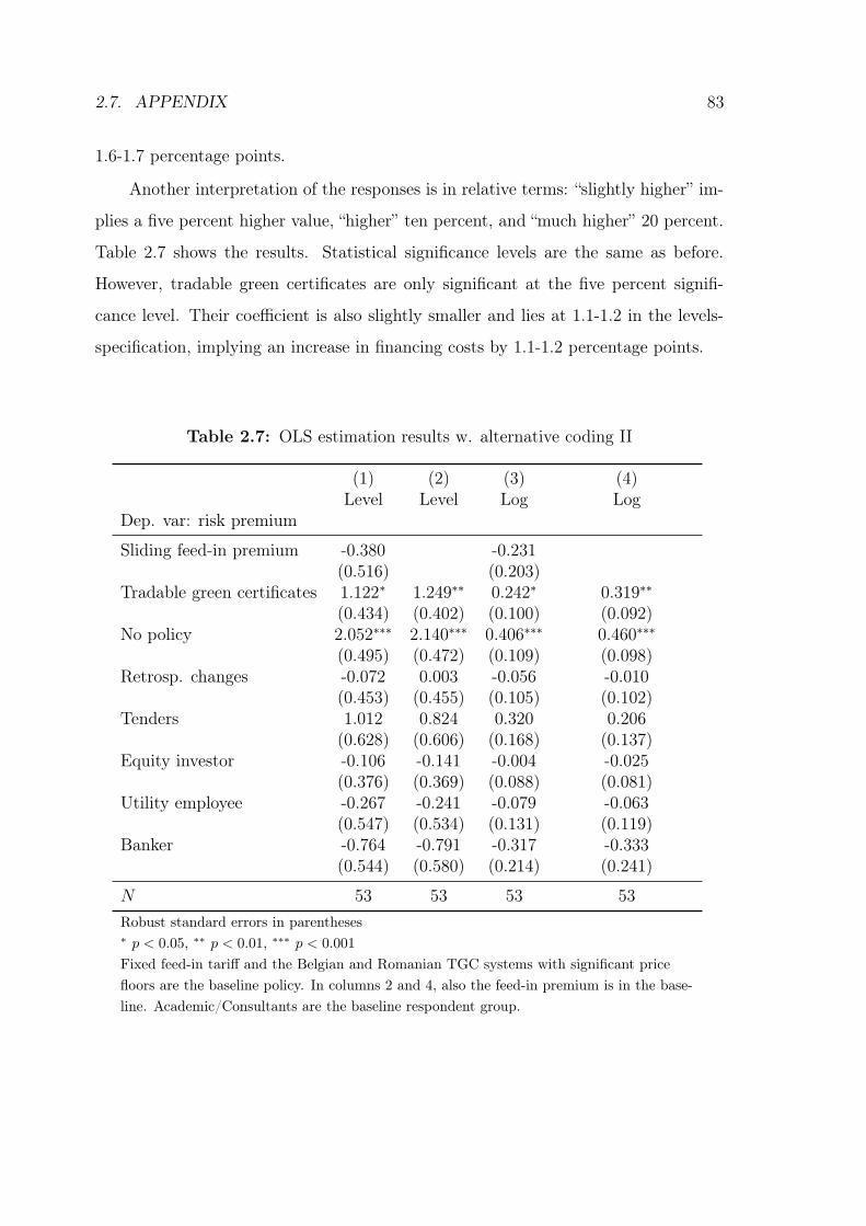
2.7. APPENDIX 83

1.6-1.7 percentage points.

Another interpretation of the responses is in relative terms: “slightly higher” im-

plies a five percent higher value, “higher” ten percent, and “much higher” 20 percent.

Table 2.7 shows the results. Statistical significance levels are the same as before.

However, tradable green certificates are only significant at the five percent signifi-

cance level. Their coefficient is also slightly smaller and lies at 1.1-1.2 in the levels-

specification, implying an increase in financing costs by 1.1-1.2 percentage points.

Table 2.7: OLS estimation results w. alternative coding II




Tradable green certificates 1.122* 1.249** 0.242* 0.319**(0.434) (0.402) (0.100) (0.092)

No policy 2.052*** 2.140*** 0.406*** 0.460***(0.495) (0.472) (0.109) (0.098)

Retrosp. changes -0.072 0.003 -0.056 -0.010(0.453) (0.455) (0.105) (0.102)

Tenders 1.012 0.824 0.320 0.206(0.628) (0.606) (0.168) (0.137)

Equity investor -0.106 -0.141 -0.004 -0.025(0.376) (0.369) (0.088) (0.081)


Banker -0.764 -0.791 -0.317 -0.333(0.544) (0.580) (0.214) (0.241)




Table 2.8: Interest rate as linear function of traded US companies’ credit ratings,based on aggregate data by Damodaran (2017)


Dep. var.: 𝑟𝑑𝑒𝑏𝑡g 0.0052989***

(0.0009123)m -0.02087331**


2.7.3 Functional form of the interest rate function

Assuming a linear functional form for the interest rate function 𝑟𝑑𝑒𝑏𝑡𝑔 , we formulate

the following function:

𝑟𝑑𝑒𝑏𝑡(𝑔(𝑑, 𝑒)) = 𝑚+ 𝜆𝑔(𝑑, 𝑒) (2.14)

with slope

∂𝑟𝑑𝑒𝑏𝑡(𝑔(𝑑, 𝑒))

∂𝑔(𝑑, 𝑒)= 𝜆 (2.15)

Equivalent to the previous estimation, we estimate:

𝑟𝑑𝑒𝑏𝑡𝑔 = 𝑚+ 𝜆𝑛𝑔 + 𝑢𝑔 (2.16)

In this case, the constant is -.0208 and the slope is 0.0052, as depicted in 2.8.

The additional costs for long-term contracts under green certificates differ ac-

cordingly, as depicted in figure 2-9. Using the exemplary cost parameters laid out

in section 2.5, an installation based on the average debt-equity ratio of the large EU

utilities of 1.85 sees additional costs of about 33.4%, i.e. considerably more than

in the quadratic case. With worse debt-equity ratios, the costs under the quadratic

functional form increase more sharply.

2.7. APPENDIX 85

Figure 2-9: Extra re-financing costs for private off-takers as share of contract valuewith linear interest rate

Chapter 3

Too Good to Be True? How

Time-Inconsistent Renewable Energy

Policies Can Deter Investments∗

Abstract

The transition towards low-carbon economies requires massive investments into re-newable energies, which are commonly supported through regulatory frameworks.Yet, governments can have incentives – and the ability – to deviate from previously-announced support once those investments have been made, which can deter invest-ments. We analyze a renewable energy regulation game, apply a model of time-inconsistency to renewable energy policy and derive under what conditions govern-ments have incentives to deviate from their commitments. We analyze the effects ofvarious support policies and deployment targets and explain why Spain conductedretrospective changes in the period 2010-2013 whereas Germany stuck to its commit-ments.

∗This chapter is based on joint work with Olga Chiappinelli. We thank Sascha Drahs, KarstenNeuhoff, and Jörn Richstein for their helpful comments and suggestions. We also benefited fromcomments by participants at the joint energy market research seminar by TU Berlin, the Ifo Institutefor Economic Research, TU Munich, the University of Nuremberg, and DIW Berlin.

87

88 CHAPTER 3. TIME-INCONSISTENCY & RENEWABLE ENERGIES

3.1 Introduction

In 2016, global investments into renewables-based power capacity outpaced invest-

ments into coal and gas power plants, amounting to e297 billion (IEA, 2017). In-

vestment needs remain high over the next decades, supporting countries’ transitions

to not just low-carbon electricity but also other energy sectors. The vast majority of

renewable energy projects are facilitated through supportive regulatory frameworks

and policies. These policies offset the usually not-internalized negative externalities

of thermal power plants and support the learning of technologies (Edenhofer et al.,

2013).

Governments support renewable energy investments by promising investors cer-

tain policy frameworks and remuneration levels. Time-inconsistency can arise as

regulators follow a multi-objective agenda: They pursue long-term decarbonization

trajectories, yet these may conflict with short term distributional concerns regarding

the costs of energy (Chiappinelli and Neuhoff, 2017). Moreover, in addition to the

desire to do so, regulators can have the ability to deviate from previously-announced

support levels since renewable energy investments are irreversible and operate at very

low marginal costs: Regulators interested in renewable energy announce support lev-

els to be paid via levies on electricity, based on which investors respond by investing

into new capacity. However, regulators then possibly deviate, not paying out the

promised support, benefiting from both the now-existing renewable energy capacity

and the low costs of electricity. Firms anticipate this opportunistic behavior and do

not invest in the first place. However, when the game is repeated, there is scope for

compliance depending on policies and technology parameters.

The monetary policy literature first applied time-inconsistency concepts to infla-

tion and economic growth. In their ground-breaking article, Kydland and Prescott

(1977) analyze unemployment and inflation and lay out the problem that rational

agents optimizing at different points in time adjust their behavior simply due to the

different timing, leading to sub-optimal outcomes when agents are rational. Barro

and Gordon (1983) underpin the argument that rules for government behavior can


have favorable outcomes rather than the discretion to adjust policies when optimal.

Subsequently, the concept has been used to analyze broader climate policies.

Helm et al. (2003) demonstrate that emission pricing faces similar problems since

agents foresee that incentives for emission reductions that are optimal ex-ante be-

come suboptimal ex-post, thus diminishing their credibility in the first place. This is

extended for different cases, e.g. where governments and firms are uncertain about

future governments’ preferences, inducing arguments for research grants (Ulph and

Ulph, 2013). Brunner et al. (2012) discuss solutions to the commitment problem

with a focus on delegation to an independent climate agency, long-term planning via

targets and securitization through legal rights. In this context, they mention feed-

in tariffs for renewable energies as favorable example and dismiss the retrospective

changes that Spain had just initiated as “unlikely to affect investors’ property” (p.16),

which has since turned out to be incorrect. Remuneration levels were cut by around

25 percent on average (Comisión Nacional de los Mercados y la Competencia, 2014,

2015).

Renewable energy policy has some common features with general environmen-

tal regulation: Demand for renewable energy is driven and affected by government

regulations. Due to their high initial capital intensity and low marginal costs, invest-

ments into wind and solar power are potentially exposed to time-inconsistency issues

as once investments are made, operators will usually operate the assets independent

of remuneration. Consequently, governments might face incentives to deviate because

existing installations will run in any case.

We contribute to the literature by scrutinizing time-inconsistency problems of

renewable energy policies in detail. Building on the analysis of time-inconsistency of

environmental regulation by Chiappinelli and Neuhoff (2017), we show that renewable

energy policies can be affected by time-inconsistency and consider different policy

regimes and how they affect regulatory compliance. As renewable energy support is

usually not paid out as capacity support, but rather over the projects’ lifetimes as

payments for output, we model the interaction between firms and the government

as a dynamic game where the effects of past periods’ support commitments and


investments last into the present.

We analyze commitment devices in the field of renewable energy. While Borgh-

esi (2011) argues that renewable energy targets, like the European 2020 renewable

energy targets can incentivize commitment, we show that targets only do so under

certain conditions. Habermacher and Lehmann (2017) analyze more generally how

uncertainty about environmental benefits leads to changing optimal support levels

over time, but do not focus on the classical commitment problem where the optimal

regulatory support differs over time even in the absence of new information.

Our analysis can explain why some countries deviate from their announced re-

newable energy support policies while others do not. For example, Spain, then a

global frontrunner in renewable energies, cut its renewable energy support over the

2010 to 2013 period, while Germany, another frontrunner, did not.

The chapter is structured as follows: Section 3.2 describes the dynamic regulatory

game. Section 3.3 characterizes optimal regulatory and firm behavior. We discuss

the effects of various renewable energy policies and targets in section 3.4. Next, in

section 3.5, we proceed to apply the model to the situations facing Spain and Germany

around 2012 to derive reasons for their differing behavior. The chapter ends with a

conclusion.

3.2 Setup of the regulation game

Regulatory support for renewable energies can be modeled as a game where the

regulator announces and sets support levels, while firms form expectations about the

anticipated support levels and choose to invest or not. A dynamic regulatory game is

a useful model of renewable energies support policies for the following reasons: First,

investments into renewable energies are capital intensive up-front, which implies that

expectations about lifetime earnings formed at the investment stage define capital

costs and, thus, the required support level (see, among others, Couture et al., 2010,

Haas et al., 2011, May, 2017). Due to the dependence of investments on support

policies, investors emphasize the importance of stable regulation without unexpected

3.2. SETUP OF THE REGULATION GAME 91

changes (Lüthi and Wüstenhagen, 2012). Only a small fraction of the costs is incurred

after the investment stage, such that installations will operate (almost) independent

of actual revenues. This matters because, secondly, renewable support is typically

paid out throughout the lifetime of the assets as support per output to incentivize

efficient project planning and management. Consequently, over the lifetime of the

assets, there is ample time for regulators to behave strategically and to deviate of

their initial support commitments because the assets will continue generating power

regardless.

The government acts as Nash leader, such that it announces a renewable energy

regime and support level that a representative firm, as Nash follower, can observe and

take into account for its investment decision. The firms invest into renewable energy

depending on the remuneration they expect.

The game modifies the more general setup introduced by Chiappinelli and Neuhoff

(2017) to take into account dynamic aspects of the interaction between the govern-

ment and the firms, depicting the renewable energy setting in more detail. Figure

3-1 visualizes the general setup. First, the government announces its support for

renewable energy. The remuneration is financed as a levy on the electricity price, to

be paid by all electricity consumers, thus decreasing the demand for electricity, as is

implemented in most European countries (Eclareon, 2017). Second, the firms choose

to invest into renewable energy capacity, generating renewable energy. Third, the

government observes the firms’ investment decisions and sets the actual remunera-

tion level. This mirrors that regulators can, if the policy design allows them to, alter

the support level after project completion, effectively changing the remuneration over

the entire lifetime of the project.

To reflect that renewable energy support is almost universally paid out per unit

of output, rather than installed capacity, the model is dynamic and actions directly

affect future periods. Support promised in period 𝑡 lasts into the next period 𝑡 + 1

and investments undertaken in 𝑡 still reduce emissions in 𝑡 + 1, after which they are

assumed to cease operating.

We adopt a linear direct demand function 𝑄𝑡 where electricity prices increase with


Regulator announces support level p

Firms choose investment level, generating x

Regulator sets actual support level p and payoffs are realized

Figure 3-1: Timing of the period game, which is repeated indefinitely

renewable energy support: Without support, demand is equal to 𝑎 and decreases by 𝑏

for every Euro of support per megawatt-hour (MWh). Support for renewable energies

𝑝 is promised for two periods,1 such that both the past period’s promised support

𝑝𝑡−1 and the present support 𝑝𝑡 influence demand in the present.

𝑄𝑡 = 𝑎− 𝑏𝑝𝑡−1 − 𝑏𝑝𝑡 (3.1)

In every period, the government optimizes welfare 𝑊𝑡 by setting the renewable

energy levy 𝑝𝑡. The regulator represents the interests of electricity customers and,

thus, cares about consumer surplus, comparable to the model setup in Salant and

Woroch (1992), but also cares about environmental pollution, as in Chiappinelli and

Neuhoff (2017). As shown in equation (3.2), per-period welfare depends on the con-

sumer surplus from the consumption of electricity (first term) and the environmental

damage caused by the production of non-renewable electricity (second term).2 Dam-

age depends on emissions from covering the demand and are reduced by generation

from renewable energies. These renewable energies are the sum of generation across

1While this can easily be increased to longer support horizons, it does not alter the nature of theresults; such that we stick to two periods for notional simplicity.

2We are interpreting the alternative to investments into renewable energy as running existingthermal plants, e.g. coal and gas power plants. The avoided costs of running these, the so-calledmerit-order effects (Ketterer, 2014), implicitly dampen the costs for renewable energy support. Inthe numerical application in section 3.5, we subtract these costs from the renewables’ support costs.

3.2. SETUP OF THE REGULATION GAME 93

all firms 𝑗,∑︀𝐽

𝑗=1 𝑥𝑗𝑡 and∑︀𝐽

𝑗=1 𝑥𝑗𝑡−1 ,3 again reflecting that previous investments im-

pact later periods. The sum is multiplied with a pollution parameter 𝑒, indicating

how polluting the non-renewable power supply is.4

𝑊𝑡 =

∫︁ 𝑝′𝑡

𝑝𝑡

𝑄(𝑧)𝑑𝑧 − 𝑒(𝑄𝑡 −𝐽∑︁

𝑗=1

𝑥𝑗𝑡 −𝐽∑︁

𝑗=1

𝑥𝑗𝑡−1) (3.2)

The maximum total support, at which electricity demand drops to zero, is given

by 𝑎𝑏. Consequently, the maximum level for 𝑝𝑡 is 𝑝′𝑡 = 𝑎

𝑏− 𝑝𝑡−1.

In the long-run, welfare is the sum of future welfare, discounted by the discount

factor 𝛿 ∈ [0, 1].

𝑊 =∞∑︁𝑠=𝑡

𝛿𝑠−𝑡

[︂ ∫︁ 𝑝′𝑠

𝑝𝑠

𝑄(𝑧)𝑑𝑧 − 𝑒(𝑄𝑠 −𝐽∑︁

𝑗=1

𝑥𝑗𝑠 −𝐽∑︁

𝑗=1

𝑥𝑗𝑠−1)

]︂(3.3)

The firms are identical competitive price-takers, representing the investment be-

havior of renewable energy investors and covering all demand. Every individual firm’s

renewable generation 𝑥𝑖𝑡 is very small compared to the sum of all firms’ generation∑︀𝐽𝑗=1 𝑥𝑗𝑡 . For simplicity, the convex cost function 𝑐(𝑥𝑖𝑡) is assumed to be quadratic

in investments, depending on some factor 𝛼 > 0, as shown in equation (3.4). Costs

occur up-front and increase with deployment because project developers might only

have capacities to implement a limited number of projects at a time and because

suitable sites are scarce. Marginal operational costs are zero.

𝑐(𝑥𝑖𝑡) =𝛼

2𝑥2𝑖𝑡 (3.4)

Each firm’s short-run profits 𝜋𝑖𝑡 are influenced by the firm’s present and past re-

newable energy investments 𝑥𝑖𝑡 and 𝑥𝑖𝑡−1 and the support per unit of output. The over-

all support payments divided by the overall new generation from renewables, 𝑝𝑡𝑄𝑡∑︀𝐽𝑗=1 𝑥𝑗𝑡

,

3Precisely, 𝑥 stands for renewable energy generation, so when discussing “investments”, we referto “the investments necessary to generate 𝑥”.

4Not all non-renewable electricity is equal. With increasing renewable energy shares, thermalpower plants with higher marginal costs, e.g. gas power plants in most of Europe, might be replacedfirst, while other plants are replaced later. We abstract from this differentiation and assume onesingle pollution parameter.


represent the support per unit of output. Stated differently, the ratio 𝑥𝑖𝑡∑︀𝐽𝑗=1 𝑥𝑗𝑡

𝑝𝑡𝑄𝑡

indicates how much of the overall support for renewable energies for new generation

in period 𝑡, 𝑝𝑡𝑄𝑡, is generated by firm 𝑖.5

𝜋𝑖𝑡 =𝑥𝑖𝑡∑︀𝐽𝑗=1 𝑥𝑗𝑡

𝑝𝑡𝑄𝑡 +𝑥𝑖𝑡−1∑︀𝐽𝑗=1 𝑥𝑗𝑡−1

𝑝𝑡−1𝑄𝑡 − 𝑐𝑡 (3.5)

In the long-run, firms’ profits are the sum of all future profits, discounted by the

discount factor 𝛿.

𝜋𝑖 =∞∑︁𝑠=𝑡

𝛿𝑠−𝑡

[︂𝑥𝑖𝑠∑︀𝐽𝑗=1 𝑥𝑗𝑠

𝑝𝑠𝑄𝑠 +𝑥𝑖𝑠−1∑︀𝐽𝑗=1 𝑥𝑗𝑠−1

𝑝𝑠−1𝑄𝑠 − 𝑐𝑖𝑠

]︂(3.6)

3.3 Regulatory optima

The government maximizes welfare by setting the support level, while the firms max-

imize profits by choosing investment levels. In the commitment benchmark, the

government has to set exactly the level it has previously announced, whereas in the

absence of commitment, it has the ability to deviate. In the absence of renewable en-

ergy investments, electricity demand is covered by conventional technologies, leading

to proportional environmental damage.6

3.3.1 Commitment benchmark

When the government can commit to a particular support level 𝑝𝑡, it can take the

firms’ reaction function∑︀𝐽

𝑗=1 𝑥𝑗𝑡(𝑝𝑡) into account for its optimization of welfare 𝑊 .

Accordingly, we solve the game by backward induction, starting with the firms’ re-

action function. When optimizing, any firm’s production is very small compared to5To ensure that levy payments by electricity consumers and pay-offs for renewable energy output

match exactly, independent of demand fluctuations, balancing accounts facilitate this inter-temporalexchange, cp. for example the German “renewable energy accounts” (Bundestag, 2016). For sim-plicity and as the management of these balancing accounts is not our focus, we abstract from themand assume that levy payments and payouts match exactly in every period.

6We assume that in the absence of any renewable investments, the government will always seta support level of zero, i.e. curbing demand is not an end in itself. Appendix 3.7.1 spells out thiscondition.

3.3. REGULATORY OPTIMA 95

overall production such that it takes the sum of production as constant. This implies

that any one firm’s action does not alter the support per output, whereas all firms’

collective investments may well change the support per output.

Deriving any firm’s profit function yields that its marginal costs, 𝛼𝑥𝑖𝑡 , must in

the optimum equal its marginal revenues, 𝑝𝑡(𝑄𝑡+𝛿𝑄𝑡+1)∑︀𝐽𝑗=1 𝑥𝑗𝑡

, which are composed of the

revenues in in the investment period and in the discounted subsequent period. The

optimal investments are thus:

𝑥*𝑖𝑡 =𝑝𝑡(𝑄𝑡 + 𝛿𝑄𝑡+1)

𝛼∑︀𝐽

𝑗=1 𝑥𝑗𝑡(3.7)

Therefore, the sum of renewable energy generation from new investments is:

𝐽∑︁𝑗=1

𝑥*𝑗𝑡 =𝑝𝑡(𝑄𝑡 + 𝛿𝑄𝑡+1)

𝛼(3.8)

Consequently, the regulator takes the firms’ investment decisions into account

when setting the optimal support level 𝑝𝑠 which maximizes welfare:

𝑊 =∞∑︁𝑠=𝑡

𝛿𝑠−𝑡

[︂ ∫︁ 𝑝′𝑠

𝑝𝑠

𝑄(𝑧)𝑑𝑧 − 𝑒(𝑄𝑠 −𝑝𝑠(𝑄𝑠 + 𝛿𝑄𝑠+1)

𝛼− 𝑝𝑠−1(𝑄𝑠−1 + 𝛿𝑄𝑠)

𝛼)

]︂(3.9)

In the optimum, the regulator sets the support level in every period such that on

the margin, the additional costs of an increase in the levy in terms of reduced consumer

surplus equal the environmental benefits of the increase of the levy. The regulator is

able do this under commitment as it knows the firms’ reaction functions and possesses

perfect foresight. Consequently, in this simple setup without new information during

the game, the regulator will optimally set the same levy in every period, 𝑝𝑡−1 =

𝑝𝑡 = 𝑝𝑡+1. Any deviation would decrease welfare. When increasing the levy from this

optimal levy, the costs of a higher levy would not be worth the resulting environmental

benefits. When decreasing the levy, welfare would be lower due to the forsaken

environmental benefits.7 Imposing the steady state yields:7In our setup, a potentially optimal alternative to the steady state exists: Consumer surplus is


𝑝* =𝑎𝛼− 𝑏𝑒𝑐− 𝑎𝑒− 𝑎𝑒𝛿

𝑏(2𝑐+ 2𝑐𝛿 − 3𝑒− 8𝑒𝛿 − 4𝑒𝛿2)(1 + 𝛿) (3.10)

Overall, investments are:

𝐽∑︁𝑗=1

𝑥*𝑗 =𝑝*𝑎− 2𝑏𝑝*

𝛼(1 + 𝛿) (3.11)

Every firm invests:

𝑥*𝑖 =𝑝*𝑎− 2𝑏𝑝*

𝛼∑︀𝐽

𝑗=1

(1 + 𝛿) (3.12)

3.3.2 Dynamic optimization: no commitment case

Without commitment, the regulator deviates from the announced support level if that

is optimal. Whether or not it is optimal depends on the strategies the players are

following: Under open loop strategies, they only consider the current period’s pay-

offs, while under trigger strategies, past actions impact future actions. We explore

how far the commitment outcome can be attained under these strategies and what

factors attainment relies on.

Open loop strategies

When the government cannot commit, it can observe the firms’ investment decisions

and choose to set the remuneration level to the level that optimizes welfare, indepen-

dent of its initial announcement. The government optimizes, taking the renewable

energy output as exogenously given.

decreased by the sum of the levy of the current and the previous period. Thus, the levy does notactually have to be equal in every individual period in order to set the marginal costs of an increaseof the levy equal to the marginal benefits of an increase of the levy; it suffices that the total per-period payments are the same. The regulator could constantly switch between a high levy in oneperiod and a low levy in the next period, such that the total per-period levy payments are the samein all periods. However, this decreases welfare due to the convexity of costs in combination withlinear demand and linear environmental damages. Besides, this seems unrealistic, as real-optionstheory indicates that potential investors would delay their investments until levies are high, see e.g.Ritzenhofen and Spinler (2016).

3.3. REGULATORY OPTIMA 97

∂𝑊

∂𝑝𝑡=

∞∑︁𝑠=𝑡

𝛿𝑠−𝑡

[︂∂

∂𝑝𝑡

∫︁ 𝑝′𝑠

𝑝𝑠

𝑄(𝑧)𝑑𝑧 − 𝑒∂𝑄𝑠

∂𝑝𝑡

]︂(3.13)

Any positive remuneration level curbs demand, which reduces consumer surplus.

The only benefits are the avoided emissions due to the lower demand. However,

we assumed that the regulator will not set a levy only in order to curb demand,

see appendix 3.7.1. Thus, the government sets the support level to zero. The firms

anticipate this and optimally choose not to invest – a classical expropriation argument

(see e.g. Williamson (1975)).

Grim trigger strategies

With trigger strategies, players are able to observe the others’ past behavior and

react. A grim trigger means that once the payers deviate, they are punished forever.

In our setup, only the regulator can deviate owing to the timing of output-based

support payments. The firms can punish by not making further investments after the

regulator has deviated from its previously-announced support. In order to sustain a

subgame perfect Nash equilibrium, a deviation may not be profitable for the regulator

at any time. For a detailed formal definition of such trigger strategies, see Chiappinelli

and Neuhoff (2017).

The regulator evaluates the overall benefits of deviating against the threat of no

new investments in the future. To this end, the government compares the welfare of

compliance 𝑊 𝑐 to the welfare if it deviates 𝑊 𝑑.

𝑊 𝑐 ≥ 𝑊 𝑑 (3.14)

∞∑︁𝑠=𝑡

𝛿𝑠−𝑡𝑊 (𝑝𝑠 = 𝑝*, 𝑥𝑖𝑠 = 𝑥*𝑖 ) ≥∞∑︁𝑠=𝑡

𝛿𝑠−𝑡𝑊 (𝑝𝑠 = 0, 𝑥𝑖𝑠=𝑡 = 𝑥*𝑖 , 𝑥𝑖𝑠�=𝑡= 0) (3.15)

Transforming yields as compliance condition:


∞∑︁𝑠=𝑡

𝛿𝑠−𝑡2𝑏𝑒𝑝* +∞∑︁

𝑠=𝑡+1

𝛿𝑠−𝑡2𝑒

𝛼(1 + 𝛿)𝑝*𝑄 ≥

∞∑︁𝑠=𝑡

𝛿𝑠−𝑡(𝑎𝑝* − 𝑏𝑝*2

) (3.16)

The left hand side of equation (3.16) represents the total discounted environmen-

tal benefits that occur under compliance. Demand is reduced when the support level

is positive, which occurs in every period with some environmental benefits captured

by 2𝑏𝑒𝑝*. In contrast, only future investments are decision-relevant because the in-

vestments in period 𝑡 have been made regardless. Thus, the environmental benefits

from renewable energies 2𝑒𝛼

(1+𝛿)𝑝*𝑄 only accrue from period 𝑡+1 onward. Naturally,

past investments’ environmental benefits also do not play a role.

The right hand side shows the benefits of deviating: consumer surplus is increased

since no more support is paid. Importantly, this already begins in period 𝑡, even

though new investments have potentially still been triggered in period 𝑡, to which the

regulator is not paying the promised support. Equivalently, the regulator also does

not pay any longer for generation from investments made in period 𝑡 − 1, which are

also still eligible to support in period 𝑡.

3.4 The role of policies and targets

We analyze the effects that different support policies and explicit renewable energy

deployment targets have on compliance, costs, and renewable energy investments.

3.4.1 Time-inconsistency under different policy regimes

Policy regimes can support commitment equilibrium outcomes even though no govern-

mental action is able to rule out deviations altogether. Yet, some policy frameworks

allow for easier changes to announced support than others. An example that is eas-

ily integrated into the model are prohibitively high costs in case of “full” deviations:

Beyond some threshold, e.g. a deviation on more than a certain share (1 − 𝛾) with

3.4. THE ROLE OF POLICIES AND TARGETS 99

𝛾 ∈ [0, 1] of commitments, firms in other sectors will also fear deviations by the

regulator, which outweighs the gains from full deviations. Depending on the policy

regime, this threshold can differ. The fear of contamination of other sectors’ invest-

ments might be larger when the initial promise of the government is stronger, as the

necessary political and legal barriers are harder to overcome. If the government is

willing to get over large barriers to deviate from its renewable energy commitments, it

might appear more likely to do so in other sectors as well. In contrast, when support

levels are not clearly defined, deviations are harder to detect and understand, and

deviations might be less likely to spread to other sectors.

The model is easily extended to incorporate limited deviations. Since the pay-

offs under compliance remain unaltered, the optimal support level 𝑝* and the optimal

investment level 𝑥*𝑖 remain the same. However, the left hand side of the compliance

inequality (3.16) – the environmental benefits of compliance – decrease. Whereas

the second term on the left hand side of equation (3.17), the environmental benefits

of new investments, does not change, the environmental benefits from a decrease

in demand actually decrease with limited deviations compared to full deviations, as

shown in equation (3.17). The simple reason is that in the first two periods after the

deviation, the levy for commitments made until the time of deviation remains at 𝛾𝑝*

rather than falling to zero. As of the second period after deviation, the levy is zero

once again and the benefits accrue just as with full deviations. Appendix 3.7.2 details

the calculations.

Similarly, the benefits of deviating in terms of reduced levy payments decrease

compared to full deviations. As of the second period after a deviation, the pay-offs are

the same as under full deviations. After deviating, some levy 𝛾𝑝* remains, rendering

deviations less attractive.

In total, compliance becomes more attractive when deviations are limited than

when regulators can fully deviate. Demand is depressed after the deviation, leading

to some environmental benefits on its own, but larger negative impacts on consumer

surplus (which holds independently of the levy 𝑝 and the remaining share 𝛾 by our

assumption of negative impacts on welfare in the absence of investments; see appendix


3.7.1). The value of the left hand side decreases less than the value of the right hand

side between equations (3.16) and (3.17).

𝑒𝑏𝛾𝑝*(2 + 𝛿) +∞∑︁

𝑠=𝑡+2

𝛿𝑠−𝑡2𝑏𝑒𝑝* +∞∑︁

𝑠=𝑡+1

𝛿𝑠−𝑡2𝑒

𝛼(1 + 𝛿)𝑝*𝑄 ≥

𝛾(1 + 𝛿)𝑎𝑝* − 𝛾2(1 +𝛿

2𝑏)𝑝*

2

+∞∑︁

𝑠=𝑡+2

𝛿𝑠−𝑡(𝑎𝑝* − 𝑏𝑝*2

) (3.17)

We differentiate between three policy frameworks: Those where deviations are

difficult for governments to implement as they must also change the constitution,

frameworks where a – simpler – change of law suffices, and, lastly, such frameworks

where only some rules need to be adjusted in order to deviate.

First, there are policy frameworks where the renewable energy policy itself stresses

that it represents a remuneration stream that will not and cannot be altered over time

and where, additionally, the constitution provides investment security through strong

grandfathering rules. In order to change the constitution, which explicitly protects

existing assets from legal changes, usually a qualified majority is required in parlia-

ment, posing a high threshold for retrospective changes of the renewable energy policy

(Jakob and Brunner, 2014). This can be the case both for feed-in tariffs and feed-in

premia. However, under feed-in premia, balancing costs remain with the investors,

rendering the rules around balancing cost assignment prone to time-inconsistency

issues (Neuhoff et al., 2016). Thus, with constitutional rights and respective poli-

cies, no full deviations are possible and 𝛾 in equation (3.17) is increased, rendering

compliance more attractive.

Second, policy frameworks provide investors with an investment environment

where regulators legally guarantee some support, but this support is not backed by

constitutional grandfathering rights. Regulators can explicitly guarantee a specific

remuneration level or a sense can prevail that overall profitability of projects is guar-

anteed, but not specific support levels. Without constitutional grandfathering rights

and specified support levels, 𝛾 in equation (3.17) is lower than under the first set of


policies.

Based on such arguments, Spanish investors who had invested before 2010 lost

their case against the Spanish government that had retrospectively cut their support

payments. The Spanish supreme court judges argued that the investors were entitled

to profitability of their investments, but not necessarily the exact level they had

initially been promised. In particular, they stated that the adjustments were in line

with “legitimate expectations” (El País, 2014). This has since been explicitly codified

in the Spanish remuneration scheme and investors are guaranteed a certain markup

over the returns of governmental long-term bonds (Spanish Ministry of Industry and

Energy and Tourism, 2014). As early as between 2004 and 2007, the policy regime

explicitly adjusted support levels based on the wholesale electricity price (Spanish

Ministry of Economic Affairs, 2004), indicating a more subtle promise of support

stability in comparison to explicit long-term stability of specific support levels.

Third, policy regimes like tradable green certificates promise remuneration streams

that can be adjusted over time without retrospective legal changes. Under green cer-

tificate schemes, the number of certificates in the system defines the value of these

certificates and, thus, the remuneration levels that renewable energies receive. Regula-

tors can devalue certificates by flooding the market, e.g. by providing new certificates

to foster new technologies. Alternatively, the regulator can decrease the demand for

certificates by lowering (or not increasing) the number of certificates that power sup-

pliers need to obtain, as was the case in Poland between 2010 and 2012 (Skarżyński,

2016) and in Romania in 2017 (Business Review, 2016). In any of these cases, the

anticipated remuneration level is lowered during the lifetime of projects without the

need for explicit retrospective legal changes. Therefore, 𝛾 in equation (3.17) is even

lower compared to the other discussed policies.

These three policy frameworks hold implications for the overall costs of renewable

energy deployment. When firms have imperfect foresight, the investment costs 𝛼

increase when retrospective changes are easier to implement. In turn, this renders

retrospective changes more likely, which increases the investment costs even further,

creating a vicious cycle. This implies that ceteris paribus policies leaving more space


for regulators to deviate lead to higher costs of deployment.8

3.4.2 Targets as commitment devices

National targets monitored or enforced by a supranational entity or the public can

impact governmental behavior and can act as commitment devices. They do not

directly affect the possibility of deviations, but they increase the costs at stake when

considering deviations. Targets from a supranational level cannot usually be changed

through changes of law at the national level. As Jakob and Brunner (2014) outline,

such costs can be in terms of reputation, described by Barro and Gordon (1983), or

financially.

The commitment benchmark changes. The firms’ profit functions are not touched

in the first stage and the reaction functions remain the same as before. Welfare under

commitment is altered, incorporating the potential fine from deviation if the target

expansion �̄� is not reached. The fine 𝑓 is multiplied with the deviation from the

investment trajectory target, �̄�.

𝑊𝑡 =

∫︁ 𝑝′𝑡

𝑝𝑡

𝑄(𝑧)𝑑𝑧 − 𝑒(𝑄𝑡 −𝐽∑︁

𝑗=1

𝑥𝑗𝑡(𝑝) −𝐽∑︁

𝑗=1

𝑥𝑗𝑡−1(𝑝)) − 𝑓 [�̄�−𝐽∑︁

𝑗=1

𝑥𝑗𝑡(𝑝) −𝐽∑︁

𝑗=1

𝑥𝑗𝑡−1(𝑝)]

(3.18)

with 𝑓 = 0 if∑︀𝐽

𝑗=1 𝑥𝑗𝑡(𝑝) +∑︀𝐽

𝑗=1 𝑥𝑗𝑡−1(𝑝) ≥ �̄�. As long as the renewable energy

target is not reached, the fine 𝑓 works similarly to the increased environmental ben-

efits of renewable energies, with the only exception that reducing demand does not

inherently decrease potential fines.9 Solving for the optimal levy in the steady state

yields as optimal levy:

𝑝*𝑡𝑎𝑟𝑔𝑒𝑡 =𝑎𝛼− 𝑏𝑒𝑐− 𝑎(𝑒+ 𝑓)(1 + 𝛿)

𝑏[2𝑐(1 + 𝛿) − (𝑒+ 𝑓)(3 + 8𝛿 + 4𝛿2)](1 + 𝛿) (3.19)

8Citizen ownership is another means to alleviate time-inconsistency issues. When the regula-tor represents the interests of electricity consumers and those consumers also constitute electricityproducers, the regulator also weighs producer surplus, reducing time-inconsistency issues.

9When targets are set relative to demand, then the additional effect occurs that reducing demandlowers the renewable energy target, which is not captured by our model.


Therefore, the levy under commitment is larger if the renewable energy target

is not already reached without target. Similarly, based on the same reaction func-

tion as before, the investment level under commitment increases. If the renewable

target is not yet reached without target, but the optimal levy and investment levels

with target yield an expansion beyond the renewable target, then the corner solution∑︀𝐽𝑗=1 𝑥𝑗𝑡(𝑝) +

∑︀𝐽𝑗=1 𝑥𝑗𝑡−1(𝑝) = �̄� maximizes welfare.

As a result, potential costs of not-achievement are added to the left hand side of

equation (3.16) if the expansion target �̄� is not reached. Inequality (3.20) provides

the compliance condition. The second term on the left hand side, the environmental

benefits of renewable energy investments, is increased by the potential benefits of

avoided fines.

∞∑︁𝑠=𝑡

𝛿𝑠−𝑡2𝑏𝑒+∞∑︁

𝑠=𝑡+1

𝛿𝑠−𝑡2(𝑒+ 𝑓)

𝛼(1 + 𝛿)𝑄 ≥

∞∑︁𝑠=𝑡

𝛿𝑠−𝑡(𝑎𝑝*𝑡𝑎𝑟𝑔𝑒𝑡 − 𝑏𝑝*2

𝑡𝑎𝑟𝑔𝑒𝑡) (3.20)

Therefore, with target, compliance becomes more likely than without targets due to

the increased benefits of renewable energies if the target is high enough. With a low

target that is over-achieved in any case, the target does not increase the levy, the

investment level, or the attractiveness of compliance.

The European Union’s renewable energy deployment targets for 2020 are poten-

tially relevant for national decision-making. In 2009, the European Union introduced

the Renewable Directive. It included binding targets for the share of energy stem-

ming from renewable energies both at the European level and at the individual coun-

try level. It specifies the share out of total energy use, incorporating the transport,

heating, cooling and the electricity sectors.

The European targets are binding at the national level. These are based on

each country’s initial share of renewable energy in 2005 and their wealth, requiring

stronger actions from wealthier member states. In 2005, Malta was the country with

the lowest share of renewable energy, 0.2 percent, which it has to increase to ten

percent by 2020, whereas the country with the second-lowest share, the UK at 1.4


percent, must increase its share to 15 percent. On the other hand, Sweden with the

highest initial share of 40.6 percent, has to increase it to 49 percent and Latvia with

the second-highest share of 32.3 percent needs to reach 40 percent. Between 2009

and 2020, there are additional non-binding targets, indicating whether countries are

on track to reaching their 2020 targets.

These national targets influence the regulatory incentives for compliance as they

might be fined by the European Commission. Alternatively, countries missing their

targets can directly pay other EU countries that over-achieve their targets for sta-

tistical transfers of renewable energies, of which the first deals were closed in 2017,

technically transferring renewable energy production from Lithuania and Estonia to

Luxembourg (European Commission, 2017a,b). Equivalently, this implies a direct

financial cost for countries that do not achieve their targets through their own renew-

able energy generation.

The 2020 targets only function as commitment devices when countries do not

possess sufficient alternatives. The sustainability of biomass matters less in some

countries (Ratarova et al., 2012). Using biomass seems to have been cheaper than

wind and solar power in many Eastern European countries. Consequently, on the one

hand, the European targets made biomass investments more attractive. On the other

hand, they did not render compliance more likely for wind and solar power in these

countries, as they can reach their targets more or less regardless of wind and solar

power deployment.

Figure 3-2 shows the growth in renewable energy generation since the baseline

year of 2005 in Bulgaria.10 Starting at an initial share of 9.4 percent of renewable

energies, it stood at 18.2 percent in 2015, an increase of 8.8 percentage points. The

share of biomass has grown significantly and together with a small uptake in hydro

power generation almost suffices to fulfill the Bulgarian 2020 target of 16 percent

(an increase of 6.6 percentage points since 2005).11 Thus, targets do not function as

10Assuming that the growth in renewable energies for heating and cooling came from biomass.11Still, some wind and solar power have been installed. However, as no sustained growth in

their capacities is required to reach the 2020 target, compliance is not attractive to the Bulgariangovernment. In 2013, it retrospectively introduced a 20 percent revenue tax for wind and solar


Figure 3-2: New generation from renewable energies since 2005 in Bulgaria, basedon Eurostat (2017b)

commitment devices when alternative, preferred technologies exist or if targets are

reached ahead of time.

In most Western European countries, electricity from wind and solar power are

the main viable renewable energy technologies to reach the 2020 targets.12 Figure

3-3 depicts the increase in renewable energy in Germany since 2005.13 Even though

biomass and other renewable energies, particularly energy from municipal waste, also

play a role, new wind and solar power is considerably more prominent than it is in

Bulgaria.

Figure 3-4 shows the growth in generation from renewable energies in Spain

since 2005. Starting at 8.4 percent in 2005, the country initially strongly increased

its renewable energy share. However, after retrospective cuts between 2010 and 2013

and the passing of a moratorium for new installations, the renewable energy share

stagnated, such that the 20 percent target for 2020 is more difficult to achieve.

power, yet not for biomass installations (Fouquet and Nysten, 2015). In parallel, it announced amoratorium for all new wind and solar power installations. The national constitutional court hassince ruled that the retrospective revenue tax was unconstitutional (Fouquet and Nysten, 2015).

12Finland and Sweden represent interesting exceptions as they have strongly increased their sharesof biomass fuels in the transport sector.

13Approximating the generation and installation data from BSW-Solar (2016), we assume thattwo-thirds of the solar thermal production of 2015 was installed after 2005, in roughly equal annualamounts. The remainder of renewable energy growth in the heating and cooling sector is assumedto come from biomass.


Figure 3-3: New generation from renewable energies since 2005 in Germany, basedon Eurostat (2017b)

Countries that can only reach their targets through long-term favorable invest-

ment environments for specific technologies are more likely to stay committed to these

technologies. If they have viable alternative technologies or reach their targets ahead

of time, the potential fines 𝑓 in equation (3.4.2) diminish. Thus, commitments are

more credible in countries that are endowed with the potential for few alternative

technologies and that lag behind enforceable, supranational targets.

Figure 3-4: New generation from renewable energies since 2005 in Spain, based onEurostat (2017b)

3.5. WHY DID SPAIN DEVIATE WHEN GERMANY DID NOT? 107

3.5 Why did Spain deviate when Germany did not?

We evaluate the time-inconsistency model for 2012 by numerically modeling the exam-

ples of Spain and Germany as these countries were frontrunners in renewable energy,

but only Spain deviated. Germany in 2012 was the global number three in terms of

installed wind power capacity and number one for solar, Spain was number four for

wind power and number five for solar power (IRENA, 2017a). With its renewable

energy payments at about e34 per MWh in 2012 (Comisión Nacional de Energia,

2012), Spain conducted retrospective changes between 2010 and 2013. Germany did

not, even though it had also experienced unprecedented growth in PV installations,

increasing the levy three-fold from e11.3 per MWh in 2009 to e36.9 per MWh in

2012 (and subsequently to e52.7 per MWh in 2013) (Bundesnetzagentur, 2017). Why

did and could Spain take these measures, whereas Germany did not?

As this analysis focuses on time-inconsistency, all past investments into renewable

energies are taken for granted and not accounted for in terms of environmental benefits

because they accrue in any case. This is also where potential time-inconsistency

arises from: As the investments before 2012 have already been made, only their

disadvantages, namely their costs, persist and matter for the decision-maker.

3.5.1 Parameters in 2012

In 2012, Spain had 22.8 GW of wind power and 6.6 GW of solar capacity, highlighting

a focus on (then cheaper) wind power. Germany had 31.3 GW of wind power capacity,

owing to rather constant growth in wind power capacities, and rather erratic growth

in PV between 2009 and 2012, when 22 GW of the PV total of 32.8 GW were installed

(IRENA, 2017a).

The policy framework sets the backdrop against which investors invest and spec-

ifies how easily retrospective changes can be conducted. After some policy changes

in the 2000s, Spain had a feed-in tariff for wind power, photovoltaics and concen-

trated solar power. Between 2004 and 2007, installations were not granted specific


remuneration levels, but multiples of the power price. This policy, based on a more

general sense of profitability as laid out in section 3.4.1, allowed some deviations.

Spain cut about 25 percent of its renewable energy payments from a total of e9.1

billion to e6.6 billion (Comisión Nacional de los Mercados y la Competencia, 2014,

2015). Since then, there have been conflicting court rulings. As detailed in section

3.4.1, the Spanish Supreme Court decided that Spanish investors were not eligible

for compensation. International investors have been deploying the Energy Charter

Treaty, which also led to different outcomes: On the one hand, one firm successfully

argued that its revenues fell by two-thirds and it was awarded compensation from

the Spanish government. On the other hand, a similar case of another firm that had

invested somewhat later was dropped on the grounds that “no reasonable investor

could have the expectation that this framework would not be modified in the future

and would remain unchanged" (Stibbe, 2017). Therefore, we assume that the Span-

ish regulators were able to cut around twenty percent of support payments, setting

𝛾 = 0.8 in equation (3.17), slightly less than the actual 25 percent, which, at least in

some cases, seems to have infringed on investors’ legal rights.

Germany had a feed-in tariff that allowed firms the option to shift to a feed-in

premium. As described in section 3.4.1, the focus of the legislation and the consti-

tutional grandfathering rights was on providing stable support. This enables only

small deviations. In order to compare factors other than the policy regime differences

between Spain and Germany, we set 𝛾 = 0.8 for Germany as well, noting that this is

an upper bound of the attractiveness of deviating.

The regulator compares the current and future benefits and costs of compliance

and deviation based on equation (3.17). The payouts are calculated for all future

periods until 2050, summing up the discounted welfare of the individual years.

Costs of renewable energy

We need to know how renewable energy generation 𝑥, costs 𝑐, power demand 𝑄, and

the renewable energy support 𝑝 develop in the future under compliance. We use a

detailed model created by Öko-Institut (2017) that provides estimates for the German


renewable energy levy, which uses installation trajectories, power demand, and costs

as inputs. In order to calculate the levy under compliance for Spain, we calculate how

large the levy would have been without deviation and add approximated extra costs

of new renewables installed after 2012 under compliance. Details of the calculations

can be found in appendix 3.7.3.

Discount factor

The discount factor 𝛿 determines the relative weight of current and future periods and

affects time-(in)consistent behavior to a large extent. Spain was at the height of the

financial crisis in 2012. The government passed austerity measures in many sectors of

the economy. Whereas the government previously filled the utility companies’ tariff

deficit, it was severely constrained to do so. We use the average Spanish ten-year

governmental bond rate, a standard indicator of the regulatory discount rate of 2012,

which was 5.9 percent (Eurostat, 2017a). In Germany, this rate was considerably

lower at 1.5 percent (Eurostat, 2017a).

Demand

In line with the model setup, we assume that demand Q is linear. We need to assume

values for 𝑎 and 𝑏. For both countries, we assume a demand slope of 𝑏 = 30 MWh2/e.

This is based on long-run inelastic demand elasticities of .16 in Germany and .3 in

Spain, obtained from Madlener et al. (2011). For example, for Germany in 2012, this

yields that a levy of e36 per MWh and at an exemplary household electricity price

without levy of e230 per MWh reduces demand by about 2.5 percent. Based on this,

we can calculate the increase in demand after a deviation, i.e. with a lowered levy.

We use the same demand slope for Spain as for Germany because Spanish demand

is lower, but the demand elasticity is almost twice as high. For Spain, this implies

that the Spanish levy of e34 per MWh decreases demand without levy by about 4.3

percent. Moreover, based on realized demand volumes and the demand elasticities,

we derive 𝑎, the demand without any levy. For Germany, this demand in 2017 was


about 361 TWh,14 whereas it stood at 239 TWh in Spain. Details on the calculations

can be found in appendix 3.7.4.

We treat the costs of renewable energies as levy in Spain as well, even though

this is only partially correct: Utility companies bore the costs, but were only partially

reimbursed through customers’ electricity bills. They were stuck with a considerable

chunk of the costs. This accumulated in a tariff deficit, which accumulated to e30

billion (Linden et al., 2014). These costs were eventually securitized and offered on the

financial market. Ultimately, these costs are borne by electricity consumers (Reuters,

2010), such that the link between costs of new investments and levy is less direct than

in Germany, but nevertheless exists.

Environmental benefits

The environmental benefits 𝑒 from renewable energies (and to a much smaller extent

from the reduction in demand) are the main factor driving and justifying renewable

energy support. For both countries, we apply a shadow carbon price of e50 per ton

of CO2. This by far exceeds the observed emission prices of the European emission

trading scheme, for which many authors argue that they insufficiently reflect the true

costs of pollution, e.g. Grubb (2012) and Edenhofer et al. (2017).

The carbon price is then multiplied with the carbon intensity for each country.

In Spain, the average carbon intensity in 2013 stood at 303 grams of carbon dioxide

equivalents per MWh (Moro and Lonza, 2017), yielding 𝑒 = 15.15 e/MWh, which

we apply for every period after 2012. In Germany, the intensity was 567 grams per

ton (Moro and Lonza, 2017), implying that the environmental benefits of reduced

conventional generation of 𝑒 = 28.35 e/MWh exceed Spain’s.

Investment volumes after 2012

In Spain, we observe a stand-still following the deviation and the simultaneously-

introduced moratorium. Thus, we do not know what installation volume a regulator14In addition, there are around 150 TWh of industry demand and self-consumption of electricity

that are mostly exempted from the renewable levy.


Figure 3-5: Drivers of the Spanish deviation. Positive values indicate that compli-ance is (rendered) more attractive, negative values that deviating is (rendered) moreattractive.

would have assumed. We choose 1500 MW for wind power, 750 MW for photovoltaics,

and no new concentrated solar power. For Germany, we use the realized installation

volumes for 2013-2016, even though those, particularly the PV boom between 2010

and 2012, certainly were not exactly expected.

Targets

As detailed in section 3.4.2, Spain and Germany were on a rather similar track toward

reaching their 2020 obligations in 2012. Spain’s renewable energy share was 14.3

percent in 2012, well on its way toward its target of 20 percent by 2020 (Eurostat,

2018). Germany’s share in 2012 was 12.1 percent, similarly far on its path to reaching

18 percent by 2020 (Eurostat, 2018).

3.5.2 Results

In Spain, deviation was more attractive than compliance by about e2 billion, whereas

in Germany compliance was more attractive by about e10 billion. Figure 3-5 visu-

alizes the effects of the main drivers: Spain’s higher discounting of future periods,


Figure 3-6: Spanish renewable energy levy, where compliance includes benefits ofthe merit-order effect of renewable energies installed after 2012

Germany’s relatively dirty fleet of conventional power plants, and Spain’s higher elec-

tricity prices implying lower extra costs for renewable energies.

The higher Spanish discount factor is able to explain a significant part of the dif-

ference between Germany and Spain. Had Germany conducted the same discounting

as Spain, deviating would have been more attractive also there. The higher discount

rate would have made deviating e45 billion more promising. The high Spanish dis-

count factor, for example, implies that pay-offs in 2020 only count 60 percent of the

pay-offs in 2012, whereas in Germany, 2020-payoffs still count 86 percent as much.

The dirty German thermal power plant fleet turns out as very relevant as well.

Germany with the Spanish thermal power plant fleet would have had large incentives

to deviate, as deviating would have been e27 billion more attractive than with the

German power plant. This also implies that Spain would not have deviated, had it

possessed the dirty German power plant fleet.

The extra costs of renewables are considerably lower in Spain, almost entirely

driven by the higher wholesale electricity price. With the low Spanish extra costs

of renewables, compliance pay-offs would have been around e60 billion higher in

Germany. Figures 3-6 and 3-7 show the renewable energy levies in Spain and Germany

under compliance and deviation, also taking into account the induced merit-order of


Figure 3-7: German renewable energy levy, where compliance includes benefits ofthe merit-order effect of renewable energies installed after 2012

new installations. In Spain, the levy after deviating is the actual Spanish levy, which

we can observe between 2012 and 2017. The levy under compliance lies higher since

on the one hand, costs have not been cut by 20 percent in 2012 and, on the other

hand, because new installations after 2012 are supported. The levy does not increase

anymore after 2013 even under compliance. The reason is the Spanish wholesale

electricity price, which stood at e44 per MWh in 2012 and increased to about e51

per MWh in 2017 (OMIE, 2018), reducing support costs as the difference between

power price level and support level decreases. In Germany, the opposite happened.

Power prices declined strongly from e55 per MWh in 2012 to around e30 per MWh

in 2017 and the levy for new investments, despite their relatively low costs, increases

somewhat until the early 2020s and only falls thereafter. Therefore, the extra costs for

renewable energies, i.e. the difference between the costs of new installations and the

power price, is much smaller in Spain, rendering compliance more attractive there.

Due to the high Spanish price level and the falling costs of renewable energies,

renewable energies become cost-competitive when considering their environmental

benefits as early as 2020 for wind power and 2029 for solar power. The date for

solar power is later since the costs consist of a combination of utility and small-

scale installations, where utility-scale solar becomes cheaper than the power price


beforehand already. In Germany, power prices are lower but environmental benefits

are larger. Wind power is cost-competitive in 2020 and the mix of utility- and small-

scale solar power in 2027.15

When adding a fine for breaching the countries’ 2020 targets, both countries be-

come more likely to comply, but the effect is considerably larger in Germany. Through

Germany’s low discount rate, the potential fines – only starting in 2020 – weigh 25

percent heavier than in Spain. While the pay-offs after 2020 represent almost three

quarters of all pay-offs in Germany, they only represent 58 percent in Spain.

3.6 Conclusion

Time inconsistency can arise for renewable energy investments and deter investments.

In light of large investment needs, it is crucial that policy-makers address time incon-

sistency issues through policy frameworks.

We develop a dynamic regulatory game where the regulator optimizes welfare

by announcing and setting renewable energy support, while firms invest in renew-

able energies. While, with open loop strategies, the regulator always deviates, trigger

strategies can induce compliance if environmental benefits of future investments out-

weigh the costs of old and new investments. Governmental behavior, thus, hinges on

the environmental benefits of future investments. If the expected renewable energy

output and its environmental pay-offs are sufficiently large and firms do not invest

after regulatory deviations, governments do not deviate from their announced policies.

Some policies make it easier for the regulator to deviate, whereas others tie the

hands of the regulator more tightly. Firstly, sliding premia and feed-in tariffs that

stress specific support levels together with grandfathering rules guaranteed by the

constitution leave the least space for regulatory deviations. Secondly, sliding premia

and feed-in tariffs with a more vague expectation of general profitability based on

certain power market characteristics, like the wholesale electricity price, give the

15Assuming that due to simultaneity of supply, renewable energies produce at only 80 percent ofthe wholesale power price.

3.6. CONCLUSION 115

regulator some flexibility with respect to remuneration levels. Through legal changes,

remuneration levels can be adjusted to a certain extent. Thirdly, green certificate

schemes provide regulators with the ability to adjust support levels ex-post more

easily still. The rules of the system, like the number of certificates for new installations

or the obligations for electricity retailers, can be adjusted relatively easily without

explicitly interfering with firms’ property rights.

Moreover, we show that national, binding deployment targets stemming from a

supranational entity like the EU can make compliance more attractive for govern-

ments as their stakes are increased. However, we also demonstrate that this holds

exclusively when only limited renewable resources are available to reach those targets

as governments can otherwise simply shift the focus to other renewables.

In a numerical application, we identify the reasons why Spain conducted retro-

spective cuts to its renewable energy support, while Germany did not. The model

suggests that on the one hand, the extra costs of renewable energies were actually

considerably lower in Spain due to the higher wholesale electricity price, rendering

compliance more attractive in Spain. However, on the other hand, this is outweighed

by the dirtier German conventional power plants, which increase the environmental

benefits of renewable energies in Germany. Most importantly, the larger myopia of

the Spanish regulator, caused by high discounting during the financial crisis of future

benefits of sustained renewable energy deployment, rendered deviating more attrac-

tive. These factors were combined with an enabling policy regime that left some space

for retrospective changes.

Questions remain how to make compliance more attractive for regulators. One

approach might be Contracts for Differences – existing in the UK – where firms have to

pay back the regulator when power prices lie above support levels. If the general power

price level increases while costs of renewables decrease, regulators have incentives

to keep renewables inside support schemes and deviating becomes less attractive.

Additionally, the effects of differing discount rates between the regulator and firms

might extend the existing analysis and allow for interesting scenario analyses.


3.7 Appendix

3.7.1 Levy condition

We assume that in the absence of investments into renewable energies, the regulator

optimally sets the levy to zero since any positive support level would decrease welfare.

The rational is that such additional levies on the electricity price might well be in

place, but they exist independently of the renewable energy levy. A simple example

is an energy efficiency levy, which seeks to curb demand, that is implemented inde-

pendently of the renewable energy levy. However, the renewable energy levy still also

curbs demand, but the regulator will only set a positive level if the investments into

renewable energies “are worth it”.

This assumption means that any increase in the levy 𝑝𝑡 that is not accompanied

by an increase in the investment level at some point has a negative impact on welfare.

As this must hold in every individual period, it also holds in the (discounted) sum of

period pay-offs. We assume the following holds in every period 𝑡:

∂𝑊𝑡

∂𝑝𝑡|( ∂𝑥∂𝑝𝑡

= 0) =∂

∂𝑝𝑡

∫︁ 𝑝′𝑡

𝑝𝑡

𝑄(𝑧)𝑑𝑧 − 𝑒∂𝑄𝑠

∂𝑝𝑡< 0 (3.21)

It follows that without investments into renewables, curbing demand decreases

consumer surplus more than it increases environmental benefits. Welfare from setting

a zero levy 𝑊𝑡(𝑥 = 0, 𝑝𝑡 = 0) is larger than welfare with any positive levy 𝑊𝑡(𝑥 =

0, 𝑝𝑡��=0) when there are no investments into renewable energies.

∫︁ 𝑝′𝑡

0

𝑄(𝑧)𝑑𝑧 − 𝑒𝑎 >

∫︁ 𝑝′𝑡

𝑝𝑡

𝑄(𝑧)𝑑𝑧 − 𝑒𝑄𝑡 (3.22)

3.7.2 Limited deviations

With limited deviations, as of period 𝑡 + 2, the pay-offs are the same as under full

deviations and only the pay-offs in 𝑡 and 𝑡 + 1 are altered. The impact of renewable

3.7. APPENDIX 117

energy investments remains the same as before in any case as no new investments

take place after a deviation.

As some share of the levy remains in place in period 𝑡 and period 𝑡 + 1, the

left hand side of equation (3.16) decreases because of the environmental benefits of

reduced demand. In period 𝑡, these benefits are 2𝑒𝑏𝛾𝑝*, i.e. per period the same as

before but multiplied with 𝛾 and, thus, lower than under full deviations. In 𝑡 + 1,

only the effect of 𝑝𝑡 prevails, which is discounted and, therefore, accrues to 𝛿𝛾𝑏𝑒𝑝*.

Analyzing the right hand side of equation (3.17), in period 𝑡, the regulator pays

out 𝛾𝑝𝑡 for investments from period 𝑡 and 𝛾𝑝𝑡−1 for investments from the previous

period. Therefore, the benefits of deviating decrease as some costs remain. The

negative effect on consumer surplus is 𝛾𝑎𝑝* − 𝛾2𝑝*2 . In period 𝑡+ 1, 𝛾𝑝𝑡−1 continues

to depress demand by 𝛾𝑎𝑝* − 12𝛾2𝑝*

2 . Demand reaches the same level as under full

deviations as of period 𝑡+ 2.

3.7.3 Levy calculation

To calculate the levy under compliance for Germany, we adjust the model in several

ways: First, we update the cost estimates for renewable energies in light of the coun-

try’s most recent auction results. Generally, this implies lower costs than previously

assumed. We assume wind onshore to cost e41 per MWh by 2025, PV on average

between small-scale roof-top installations and ground-mounted installations e67 per

MWh and offshore wind power e45 per MWh. Following Öko-Institut (2017), the

new installations follow the national target corridors of 2500 MW of onshore wind

power annually, 2500 MW photovoltaics, and a total of 14 GW of offshore wind power

capacity between 2017 and 2030. We assume that after 2035 support is no longer re-

quired, simplifying the calculations and resembling the current cost trends. Knowing

the support lifetimes of the new installations through 2035, we can derive the support

levels until 2050.

For Spain, we combine data from multiple sources to derive the potential renew-

able energy levy until 2050: we assume a simplistic capacity expansion of 1500 MW


of new wind power and of 750 MW of PV per year, roughly reflecting the higher

national weight on wind power deployment and the lower overall installation volume

than in Germany. The deployment costs are derived from differences in costs in 2012:

New wind power installations were about four percent more expensive per kWh in

Spain than in Germany, PV was 16 percent more expensive. Spanish wind and solar

conditions are superior to Germany’s, but the policy regime leaves more room for

retrospective changes, thus increasing the costs of financing.

Renewable energy generation reduces the overall power price. We impute this

implicit merit order effect, which dampens the renewable energy levy. Cludius et al.

(2014) show that in 2015, Germany’s 176 TWh of renewable energy generation damp-

ened the power price by about e15. This effect varies with the generation mix and the

flexibility of the system. For simplicity, we assume the merit order effect of e0.085

per TWh as constant.16 We add this merit-order effect to the renewable energy levy

in order to capture the entire electricity price effect of renewable energies.

3.7.4 Demand calculation

Following Öko-Institut (2017), German demand develops until 2021 according to the

TSO’s trend scenario (Energy Brainpool, 2014, Leipziger Institut für Energie, 2016,

Prognos, 2014); i.e. the demand paying the renewable levy decreases slightly from 356

TWh in 2016 to 322 TWh in 2021. We assume subsequent demand remains constant

due to the counter-acting effects of increased energy efficiency and self-consumption

of PV power, on the one hand, and electrification of the transport and heating and

cooling sectors, on the other hand. However, these values are realized demand values

that take into account the existing renewable energy levy. Accordingly, we calculate

the demand level without renewable energy levy, 𝑎.

In 2015 and, thus, after the deviation, Spanish demand was 232 TWh (Eurostat,

2018), which we for simplicity assume as constant in the following years. Calculating

16Spain’s electricity sector is smaller than Germany’s, thus, we would expect a larger merit-ordereffect there. However, to the authors’ best knowledge, no existing research analyzed both countries’merit-order effects with one approach. Analyses with different methodologies reach vastly differentresults, e.g. Gelabert et al. (2011) and Sáenz de Miera et al. (2008), who find much larger effects.

3.7. APPENDIX 119

the electricity demand under compliance needs to be done vice versa as Spain did

deviate in the early 2010s, such that the realized demand is based on a levy that

is already reduced by 20 percent. We start with the realized demand values, based

on Eurostat (2018), which gives us the demand Q after deviation. Knowing the

renewable energy levy 𝑝 under deviation and compliance and 𝑏, we can thus calculate

how large demand would have been without deviation. For example, Q would have

been 229 TWh in 2015.

General Conclusion

This dissertation addresses the financing and integration of renewable energies. Chap-

ter 1 demonstrates that system-friendly wind power facilitates an easier integration

of large shares of intermittent renewable energies and analyzes the incentives that

investors have to install such technologies. Chapter 2 finds empirical evidence that fi-

nancing costs differ across renewable energy support policies and identifies additional

deployment costs that occur with private long-term contracts for renewable energy.

Chapter 3 analyzes potential time-inconsistency issues, addresses how policy design

and deployment targets can alleviate them and scrutinizes the reasons why Spain had

incentives to conduct retrospective changes around 2012 while Germany did not.

Chapter 1 finds that system-friendly renewable energy technologies become more

important in power systems with higher shares of intermittent renewables. With more

wind and solar power, the technology with the lowest costs may no longer minimize

overall costs. Electricity prices decrease when it is windy in power systems designed

around thermal power plants. System-friendly technologies counter this effect, as they

have a larger share of their production in times of low wind. Therefore, in energy

systems with high shares of intermittent renewables, more system-friendly turbines

are system-optimal, i.e. minimize overall costs, than in systems with lower shares of

renewable energies.

The German sliding feed-in premium provides some incentives for system-friendly

choices, as shown both analytically and numerically, but does not transmit sufficient

incentives to install system-optimal technologies. On the one hand, system-friendly

technologies that run less simultaneously with all other wind power receive a higher

121

122 GENERAL CONCLUSION

total support. On the other hand, though, market price signals remain suppressed in

order to keep additional risks from price exposure in check. Moreover, when investors

lack perfect foresight, incentives are even less system-optimal.

Based on the system-optimality criterion, a policy designed to align private in-

centives with system-optimality while keeping revenue risks low is analyzed. Support

levels are adjusted by installation-specific adjustment factors, representing the re-

spective expected production values. System-friendly installations receive bonuses,

whereas conventional installations receive penalties. Thus, investors can consider the

entire additional expected production values of system-friendly technologies without

facing additional revenue risks during the installations’ lifetimes. This requires the

regulator to provide an expected power price profile. Further discussions of this ap-

proach, including an extension to facilitate also system-optimal locational choices, can

be found in Neuhoff et al. (2017). Questions of political acceptance of the proposed

reference-yield model arise, which future research might address. Large-scale power

system models that are detailed enough to include the specific actions of individual

investors, e.g. regarding differentiated turbine technology investment choices, would

facilitate comparing the differences to current and alternative policies in more detail.

However, such large-scale energy system models are usually not detailed enough to

analyze the incentives of individual players, let alone model important aspects like

imperfect foresight, risk-aversion, specific financing costs, or investors’ heterogeneous

requirements in terms of risk-return profiles. Additionally, large-scale models com-

monly do not allow actors to choose between several investment alternatives in terms

of technologies, as investment models like the approach in chapter 1 do, or in terms

of timing of the investment, as the real-options literature does.

The analysis in chapter 2 consists of two parts: an empirical analysis focusing

on empirically testing the impact of renewable energy support policies on wind power

financing costs and an analytical approach concentrating on the implications of long-

term contracts between investors and private off-takers. The empirical analysis finds

evidence that green certificate schemes are associated with financing costs that are

around 1.2 percentage points higher than those for feed-in tariffs and sliding feed-

123

in premia. The main reasons, frequently discussed in the literature, are the higher

revenue risks due to the uncertainty of wholesale power prices and certificate values.

The additional risks of sliding feed-in premia compared to feed-in tariffs appear to

be evaluated as rather low, which might, however, change in the future. The analysis

does not support a statistical difference in financing costs between the two policies,

even though sliding feed-in premia expose investors to some revenue risks and risks

linked to the future development of power markets, e.g. the development of balancing

costs.

In the absence of implicit long-term contracts between investors and consumers,

private long-term contracts induce additional deployment costs. Sliding feed-in pre-

mia and feed-in tariffs represent implicit long-term contracts between investors and

consumers, backed and facilitated by the regulator. Under green certificate schemes,

as well as with investments based solely on the electricity price, no such implicit con-

tracts exist. Private long-term contracts between investors and off-takers, frequently

large utility companies, aim to take over their role. Credit rating agencies count such

contracts as liabilities on off-takers’ balance sheets, such that the off-takers’ financial

ratios worsen. Consequently, their re-financing costs increase, leading to potentially

substantial implicit costs of the long-term contracts. This reduces their demand for

long-term contracts, lowers the price of these contracts below the expected power

price, increases the revenues required by investors additionally to the contracts, and,

consequently, increases overall deployment costs. These effects are larger when the

off-takers, typically large utility companies, are financially constrained. Considering

European utilities’ financial situations, we estimate that the overall costs of green

certificate schemes are around 30 percent higher than the costs under feed-in pre-

mia and feed-in tariffs. Future research could estimate the extra costs of private

long-term contracts empirically when more data on contracted volumes and contract

conditions becomes available. Moreover, if more data on financing costs, e.g. over

time, was known, also changes in effects of support policies on financing costs could

be investigated.

Chapter 3 demonstrates, analyzing the dynamic game between the regulator and


renewable energy investors, that time-inconsistency issues can arise for renewable en-

ergy investments. Regulators can have incentives to revoke previous support promises

after investments have been made in order to benefit from new installations and low

electricity prices. In an open loop game, where players only consider the current pe-

riod, no compliance can be attained since the regulator anticipates no disadvantages

when deviating. As firms foresee this, no investments are made in the first place.

Trigger strategies, i.e. where players react to other players’ previous actions and take

future consequences into account, can sustain commitment outcomes depending on

a variety of factors, including the regulator’s discount rate, costs of old installations,

costs of new installations, the wholesale electricity price level, and the environmental

benefits of renewable energy deployment.

We show that support policies and deployment targets can support the attain-

ment of commitment outcomes. Policies granting investors legal rights to specific

support levels, combined with constitutional grandfathering rights, decrease the reg-

ulator’s pay-offs when deviating and thus render compliance more attractive. Feed-in

premia, unlike feed-in tariffs, leave some limited space for adjustments, as structural

changes to balancing costs and general power market design questions can impact re-

newable energy operators. Moreover, systems where “general profitability” is stressed,

rather than specific support levels, leave more space for retrospective changes. Green

certificate schemes make adjustments even easier as they can be implemented through

rather simple changes to the number of certificates in circulation or the obligations

for retail companies. Besides, deployment targets support commitment when they

are technology-specific or few alternative technologies exist.

A numerical example identifies the reasons why Spain conducted retrospective

changes around 2012 while Germany did not. On the one hand, in Spain, the regulator

valued the long-term benefits of sustained renewable energy expansion much less due

to its high discount rate as the country was severely financially constrained. On the

other hand, Germany faced very low interest rates, leading to high valuations of future

pay-offs. Additionally, the environmental benefits differ: Germany’s existing power

plant fleet emitted considerably more carbon dioxide than Spain’s, increasing the

125

benefits of renewable energies in Germany. However, these differences are partially

countered by the much higher Spanish power prices, implying lower extra costs for

renewable energies. In sum, the model confirms that retrospective changes were

more attractive than compliance in Spain, whereas in Germany, compliance was more

attractive than deviating. Once more cases against the Spanish government have been

closed, future research could analyze how profitable the retrospective changes have

after all been for the Spanish government.

With falling deployment costs, the costs of renewable energies come closer to

power prices and in some periods and countries even lie below them, raising a set of

open research questions. When the reference price under conventional sliding feed-in

premia falls below the long-term expected power price, an increasing share of revenues

is subject to price risks. Costs covered through revenues from these uncertain revenues

above the reference price are difficult to finance through debt. Consequently, project

developers might need to secure private long-term contracts with off-takers for these

revenues or use equity to finance these costs, both increasing overall deployment

costs and possibly posing barriers to entry for small players. Alternatively, two-sided

sliding premia, like the UK’s Contracts for Differences, oblige operators to repay

the regulator when power prices are high, such that revenues are fixed in advance.

However, project developers then potentially have incentives to abstain from any

support and sell their output via private long-term contracts. Questions arise as to

how these two systems, installations both within and outside the support system, can

co-exist, as well as how these systems influence each other, e.g. how to steer volumes

in order to fulfill deployment targets. Another open question is how large the demand

for such long-term contracts is; i.e. how large a market outside the support system

can become.

The evolution of the power price signal leads to another set of open research

questions. On the one hand, in the long-term, power prices might increase, as de-

mand for electricity picks up due to the coupling of sectors, higher carbon prices and

power systems becoming more flexible. On the other hand, the value of wind and so-

lar power production might continue to fall because of their simultaneous production,


aggravated by the increasing shares of renewable energies. In any case, if the power

price fluctuates more strongly between times with wind and sun and times without,

the questions of time and location of production become ever more important. This

also raises the question of how the locational choices of investors should be managed:

Administratively, as currently the case for wind power in Germany, through the ex-

pected value of output at different locations, as sketched in Neuhoff et al. (2017), not

at all as the case in most countries, or via the splitting of price zones and respective

exposure to power prices. This showcases that with evolving power markets and with

technologies that exhibit learning, both renewable energy support policies and power

market design need to be addressed in order to facilitate the transformation to a

carbon-neutral energy system.

Bibliography

50Hertz, Amprion, TenneT, and TransnetBW. 2013. NetzentwicklungsplanStrom 2013: Zweiter Entwurf. Berlin, Dortmund, Bayreuth, Stuttgart.

AG Energiebilanzen. 2015. Stromerzeugung nach Energieträgern 1990 - 2015.Berlin.

Aïd, René, Gilles Chemla, Arnaud Porchet, and Nizar Touzi. 2011. “Hedgingand Vertical Integration in Electricity Markets.” Management Science, 57(8): 1438–1452, DOI: http://dx.doi.org/10.1287/mnsc.1110.1357.

Baringa. 2013. Power Purchase Agreements for independent renewable generators –an assessment of existing and future market liquidity. London, commissioned bythe UK’s Department of Energy and Climate Change.

Barro, Robert J., and David B. Gordon. 1983. “A positive theory of monetarypolicy in a natural rate model.” The Journal of Political Economy, 91(4): 589–610,DOI: http://dx.doi.org/http://doi.org/10.1086/261167.

BDEW. 2018. Investitionsrahmen für den Erneuerbare-Energien-Ausbau. Berlin.

Bloomberg New Energy Finance. 2016. Corporate renewable energy procure-ment.(December): .

Boomsma, Trine Krogh, and Kristin Linnerud. 2015. “Market and policy riskunder different renewable electricity support schemes.” Energy, 89: 435–448, DOI:http://dx.doi.org/10.1016/j.energy.2015.05.114.

Borghesi, Simone. 2011. “The European emission trading scheme and renewableenergy policies: credible targets for incredible results?.” International Journal ofSustainable Economy, 3(3): 312–327, DOI: http://dx.doi.org/http://doi.org/10.1504/IJSE.2011.041108.

Brunner, Steffen, Christian Flachsland, and Robert Marschinski. 2012.“Credible commitment in carbon policy.” Climate Policy, 12(2): 255–271, DOI:http://dx.doi.org/10.1080/14693062.2011.582327.

BSW-Solar. 2016. Statistische Zahlen der deutschen Solarwärmebranche (Solarther-mie). Berlin.

127

http://dx.doi.org/10.1287/mnsc.1110.1357

http://dx.doi.org/http://doi.org/10.1086/261167

http://dx.doi.org/10.1016/j.energy.2015.05.114

http://dx.doi.org/http://doi.org/10.1504/IJSE.2011.041108

http://dx.doi.org/http://doi.org/10.1504/IJSE.2011.041108

http://dx.doi.org/10.1080/14693062.2011.582327

128 BIBLIOGRAPHY

Bundesnetzagentur. 2017. EEG-Umlage: Was ist die EEG-Umlage undwie funktioniert sie?. https://www.bundesnetzagentur.de/SharedDocs/FAQs/DE/Sachgebiete/Energie/Verbraucher/Energielexikon/EEGUmlage.html(last accessed 15.02.2018).

Bundesnetzagentur. 2018a. Beendete Ausschreibungen 2017. Bonn.

Bundesnetzagentur. 2018b. Bundesnetzagentur - Gebotsermin 1. Februar2018 (Windenergie an Land). https://www.bundesnetzagentur.de/DE/Sachgebiete/ElektrizitaetundGas/Unternehmen_Institutionen/Ausschreibung-en/Wind_Onshore/Gebotstermin_01_02_2018/Gebotstermin_01_02_18_node.html (last accessed 02.03.2018).

Bundestag. 2014. Gesetz zur grundlegenden Reform des Erneuerbare-Energien-Gesetzes und zur Änderung weiterer Bestimmungen des Energiewirtschaftsrechts.Bundesgesetzblatt Teil I Nr. 33: 1066–1132.

Bundestag. 2016. Gesetz zur Einführung von Ausschreibungen für Strom auserneuerbaren Energien und zu weiteren Änderungen des Rechts der erneuerbarenEnergien. Bundesgesetzblatt Teil I Nr. 49: 2258–2357.

Bürer, Mary Jean, and Rolf Wüstenhagen. 2009. “Which renewable energypolicy is a venture capitalist’s best friend? Empirical evidence from a survey ofinternational cleantech investors.” Energy Policy, 37(12): 4997–5006, DOI: http://dx.doi.org/10.1016/j.enpol.2009.06.071.

Business Review. 2016. Romania’s renewable energy quota slashed to8.3 pct in 2017, according to government decision. http://www.business-review.eu/news/romanias-renewable-energy-quota-slashed-to-8-3-pct-in-2017-according-to-government-decision-127508 (last accessed 19.12.2017).

Butler, Lucy, and Karsten Neuhoff. 2008. “Comparison of feed-in tariff, quotaand auction mechanisms to support wind power development.” Renewable Energy,33(8): 1854–1867, DOI: http://dx.doi.org/10.1016/j.renene.2007.10.008.

CDU, CSU, and SPD. 2018. Koalitionsvertrag. Berlin.

Chiappinelli, Olga, and Karsten Neuhoff. 2017. Time-Consistent Carbon Pric-ing. DIW Discussion Paper 1710.

Cludius, Johanna, Hauke Hermann, Felix Chr Matthes, and VerenaGraichen. 2014. “The merit order effect of wind and photovoltaic electricity gener-ation in Germany 2008–2016: Estimation and distributional implications.” EnergyEconomics, 44: 302–313, DOI: http://dx.doi.org/10.1016/j.eneco.2014.04.020.

Comisión Nacional de Energia. 2012. Memoria de actividadese 2012. Madrid.

http://dx.doi.org/10.1016/j.enpol.2009.06.071


http://dx.doi.org/10.1016/j.renene.2007.10.008

http://dx.doi.org/10.1016/j.eneco.2014.04.020


BIBLIOGRAPHY 129

Comisión Nacional de los Mercados y la Competencia. 2014. Liquidaciónprovisonal de las primas equivalentes, primas, incentivos y complementos a lasinstalaciones de producción de energía eléctrica en régimen especial. Madrid.

Comisión Nacional de los Mercados y la Competencia. 2015. Informe sobrelos resultados de la liquidación provisional 14 de 2014 de la retribución de las in-stalaciones de producción de energías renovables, cogeneración y residuos. Madrid.

Couture, Toby D, Karlynn Cory, and Emily Williams. 2010. A Policymaker’sGuide to Feed-in Tariff Policy Design. NREL Technical Reports, DOI: http://dx.doi.org/NREL/TP-6A2-44849.

Couture, Toby, and Yves Gagnon. 2010. “An analysis of feed-in tariff remunera-tion models: Implications for renewable energy investment.” Energy Policy, 38(2):955–965, DOI: http://dx.doi.org/10.1016/j.enpol.2009.10.047.

Damodaran, Aswath. 2017. Ratings, Interest Coverage Ratios and Default Spread.http://pages.stern.nyu.edu/˜adamodar/New_Home_Page/datafile/ratings.htm(last accessed 20.10.2017).

Datastream International. 2016. Debt/Equity Ratio. Datastream Databank (lastaccessed 24.05.2016).

Deutsche WindGuard. 2013. Kostensituation der Windenergie an Land inDeutschland. Varel.

Deutsche WindGuard. 2014. Vergütung von Windenergieanlagen über das Referen-zertragsmodell. Varel, commissioned by Agora Energiewende.

Deutsche WindGuard. 2015. Status des Windenergieausbaus an Land in Deutsch-land 2014. Varel.

Deutscher Wetterdienst. 2016. Climate Data Germany: Wind. Offenbach.

Deutsches Institut für Bautechnik. 2012. Richtlinie für Windenergieanlagen:Einwirkungen und Standsicherheitsnachweise für Turm und Gründung. Berlin.

Deutsches Zentrum für Luft-und Raumfahrt. 2014. Möglichkeiten und Grenzendes Lastausgleichs durch Energiespeicher, verschiebbare Lasten und stromgeführteKWK bei hohem Anteil fluktuierender erneuerbarer Stromerzeugung. Stuttgart.

Diacore. 2015. The impact of risks in renewable investments and the role of smartpolicies. Ecofys, eclareon, Fraunhofer ISI, EPU-NTUA, LEI and TU Wien.

Eclareon. 2017. Res-legal: Renewable energy policy data base and support.http://www.res-legal.eu (last accessed 11.01.2018).

http://dx.doi.org/NREL/TP-6A2-44849

http://dx.doi.org/NREL/TP-6A2-44849


130 BIBLIOGRAPHY

Edenhofer, Ottmar, Christian Flachsland, Christoph Wolff, Lisa K.Schmid, Anna Leipprand, Nicolas Koch, Ulrike Kornek, and MichaelPahle. 2017. Decarbonization and EU ETS Reform: Introducing a price floor todrive low-carbon investments. Berlin.

Edenhofer, Ottmar, Lion Hirth, Brigitte Knopf, Michael Pahle, SteffenSchlömer, Eva Schmid, and Falko Ueckerdt. 2013. “On the economics ofrenewable energy sources.” Energy Economics, 40: S12–S23, DOI: http://dx.doi.org/10.1016/j.eneco.2013.09.015.

El País. 2014. Supreme Court backs cuts to solar power producers’ earnings.https://elpais.com/elpais/2014/01/21/inenglish/1390306709_143350.html (lastaccessed 15.12.2017).

Elton, Edwin J., Martin J. Gruber, Deepak Agrawal, and ChristopherMann. 2001. “Explaining the rate spread on corporate bonds.” Journal of Finance,56(1): 247–277, DOI: http://dx.doi.org/10.1111/0022-1082.00324.

Enercon. 2012. Enercon product overview. Aurich.

Energy Brainpool. 2014. Ermittlung des Marktwertes der deutschlandweiten Strom-erzeugung aus regenerativen Kraftwerken. Berlin, commissioned by TenneT TSOGmbH.

ENTSO-E. 2012. 10-Year Network Development Plan 2012. Brussels.

Estonian Windpower Association. 2015. Estonian wind en-ergy producers to receive EUR 32.2 mln of support in 2015.http://www.tuuleenergia.ee/en/2015/12/estonian-wind-energy-producers-to-receive-eur-32-2-mln-of-support-in-2015 (last accessed 20.06.2017).

European Commission. 2017a. Agreement on statistical transfersof renewable energy amounts between Lithuania and Luxembourg.https://ec.europa.eu/info/news/agreement-statistical-transfers-renewable-energy-amounts-between-lithuania-and-luxembourg-2017-oct-26_en (last accessed05.11.2017).

European Commission. 2017b. Second agreement on statistical trans-fers of renewable energy amounts between Estonia and Luxembourg.https://ec.europa.eu/info/news/second-agreement-statistical-transfers-renewable-energy-amounts-between-estonia-and-luxembourg-2017-nov-13_en (last accessed20.11.2017).

European Energy Exchange. 2016. EEX data. Leipzig.

European Union. 2009. “Directive 2009/28/EC of the European Parliament and ofthe Council.” Official Journal of the European Union.

Eurostat. 2017a. Long term government bond yields. Luxembourg.



http://dx.doi.org/10.1111/0022-1082.00324

BIBLIOGRAPHY 131

Eurostat. 2017b. Short Assessment of Renewable Energy Sources 2015. Luxembourg.

Eurostat. 2018. Supply, transformation and consumption of electricity - annual data.Luxembourg.

Finon, Dominique. 2008. “Investment risk allocation in decentralised electricitymarkets. The need of long-term contracts and vertical integration.” OPEC EnergyReview, 32(2): 150–183, DOI: http://dx.doi.org/10.1111/j.1753-0237.2008.00148.x.

Finon, Dominique. 2011. “Investment and Competition in Decentralized ElectricityMarkets: How to overcome market failure by market imperfections?.” In Competi-tion, Contracts and Electricity Markets: A New Perspective.

Fouquet, Dörte, and Jana V. Nysten. 2015. Policy Briefing: Retroactive andretrospective changes and moratoria to RES support. Keep on Track 2020!, Berlin.

Fraunhofer ISE. 2014. Effekte regional verteilter ausgerichteter Solarstromanlagen.Freiburg im Breisgau, comissioned by Agora Energiewende.

Fraunhofer IWES. 2013a. Entwicklung der Windenergie in Deutschland. Kassel.

Fraunhofer IWES. 2013b. Wie wird sich die Windenergietechnik in Deutschlandweiterentwickeln?. Kassel, commissioned by Agora Energiewende.

Fraunhofer IWES. 2015. Windenergie Report Deutschland 2014. Kassel.

Gawel, Erik, and Alexandra Purkus. 2013. “Promoting the market and systemintegration of renewable energies through premium schemes - A case study of theGerman market premium.” Energy Policy, 61: 599–609, DOI: http://dx.doi.org/10.1016/j.enpol.2013.06.117.

Gelabert, Liliana, Xavier Labandeira, and Pedro Linares. 2011. “An ex-postanalysis of the effect of renewables and cogeneration on Spanish electricity prices.”Energy Economics, 33: S59–S65, DOI: http://dx.doi.org/10.1016/j.eneco.2011.07.027.

German Ministry for Economic Affairs and Energy. 2017. Strom 2030. Berlin.

González, Javier Serrano, and Roberto Lacal Arántegui. 2015. The regulatoryframework for wind energy in EU Member States. European Commission, JointResearch Centre, Institute for Energy and Transport, DOI: http://dx.doi.org/10.2790/282003.

Grothe, Oliver, and Felix Müsgens. 2013. “The influence of spatial effects onwind power revenues under direct marketing rules.” Energy Policy, 58: 237–247,DOI: http://dx.doi.org/10.1016/j.enpol.2013.03.004.

Grubb, Michael. 2012. Strengthening The EU ETS Creating a stable platform forEU energy sector investment. Climate Strategies, London.

http://dx.doi.org/10.1111/j.1753-0237.2008.00148.x

http://dx.doi.org/10.1111/j.1753-0237.2008.00148.x





http://dx.doi.org/10.2790/282003

http://dx.doi.org/10.2790/282003


132 BIBLIOGRAPHY

Haas, Reinhard, Gustav Resch, Christian Panzer, Sebastian Busch, MarioRagwitz, and Anne Held. 2011. “Efficiency and effectiveness of promotionsystems for electricity generation from renewable energy sources - Lessons fromEU countries.” Energy, 36(4): 2186–2193, DOI: http://dx.doi.org/10.1016/j.energy.2010.06.028.

Habermacher, Paul, and Paul Lehmann. 2017. Commitment vs. Discretion inClimate and Energy Policy. Cesifo Working Paper 6355.

Hau, Erich. 2014. Wind Resources. Berlin, Heidelberg. Springer, DOI: http://dx.doi.org/10.1007/978-3-642-28877-7.

Helm, Dieter, Cameron Hepburn, and Richard Mash. 2003. “Credible carbonpolicy.” Oxford Review of Economic Policy, 19(3): 438–450, DOI: http://dx.doi.org/10.1093/oxrep/19.3.438.

Helm, Dieter, Richard Mash, and Cameron Hepburn. 2004. Time inconsis-tent environmental policy and optimal delegation. Oxford University Departmentof Economics, Working Paper 175.

Helms, Thorsten, Sarah Salm, and Rolf Wüstenhagen. 2015. “Investor-Specific Cost of Capital and Renewable Energy Investment Decisions.” In RenewableEnergy Finance - Powering the Future. ed. by Charles W. Donovan, London: Im-perial College Press, 77–101, DOI: http://dx.doi.org/10.1142/9781783267774_0004.

Hirth, Lion. 2013. “The market value of variable renewables.” Energy Economics,38: 218–236, DOI: http://dx.doi.org/10.1016/j.eneco.2013.02.004.

Hirth, Lion, and Simon Müller. 2016. “System-friendly wind power. How ad-vanced wind turbine design can increase the economic value of electricity generatedthrough wind power.” Energy Economics, 56: 51–63, DOI: http://dx.doi.org/10.1016/j.eneco.2016.02.016.

IEA. 2017. “World Energy Outlook 2017.” DOI: http://dx.doi.org/10.1016/0301-4215(73)90024-4.

IPCC. 2014. Climate Change 2014: Synthesis Report. Contribution of WorkingGroups I, II and III to the Fifth Assessment Report of the Intergovernmen-tal Panel on Climate Change. Core Writing Team, R.K. Pachauri and L.A.Meyer (eds.). IPCC, Geneva, Switzerland, DOI: http://dx.doi.org/10.1017/CBO9781107415324.

IRENA. 2017a. Renewable capacity statistics 2017. Abu Dhabi.

IRENA. 2017b. Untapped potential for climate action: Renewable energy in Nation-ally Determined Contributions. Abu Dhabi.



http://dx.doi.org/10.1007/978-3-642-28877-7

http://dx.doi.org/10.1007/978-3-642-28877-7

http://dx.doi.org/10.1093/oxrep/19.3.438

http://dx.doi.org/10.1093/oxrep/19.3.438

http://dx.doi.org/10.1142/9781783267774_0004

http://dx.doi.org/10.1142/9781783267774_0004




http://dx.doi.org/10.1016/0301-4215(73)90024-4

http://dx.doi.org/10.1016/0301-4215(73)90024-4

http://dx.doi.org/10.1017/CBO9781107415324

http://dx.doi.org/10.1017/CBO9781107415324

BIBLIOGRAPHY 133

IWR. 2018. EEG-Mindestvergütungssätze 2004-2008. http://www.iwr.de/re/wf/eegphotovoltaik.htm (last accessed 15.01.2018).

Jakob, Michael, and Steffen Brunner. 2014. “Optimal Commitment Under Un-certainty: Adjustment Rules for Climate Policy.” Strategic Behavior and the Envi-ronment, 4(3): 291–310, DOI: http://dx.doi.org/10.1561/102.00000047.

Joskow, Paul. 2011. “Comparing the Costs of Intermittent and Dispatchable Elec-tricity Generating Technologies.” American Economic Review, Papers and Proceed-ings of the One Hundred Twenty Third Annual Meeting of the American EconomicAssociation, 101(3): 238–241, DOI: http://dx.doi.org/10.1257/aer.100.3.238.

Joskow, Paul L. 2006. “Competitive electricity markets and investment in newgenerating capacity.” Working Papers 0609, Massachusetts Institute of Technology,Center for Energy and Environmental Policy Research.

Ketterer, Janina C. 2014. “The impact of wind power generation on the electricityprice in Germany.” Energy Economics, 44: 270–280, DOI: http://dx.doi.org/10.1016/j.eneco.2014.04.003.

Kitzing, Lena. 2014. “Risk implications of renewable support instruments: Compar-ative analysis of feed-in tariffs and premiums using a mean-variance approach.” En-ergy, 64: 495–505, DOI: http://dx.doi.org/10.1016/j.energy.2013.10.008.

Klobasa, Marian, Jenny Winkler, Frank Sensfuss, and Mario Ragwitz.2013. “Market Integration of Renewable Electricity Generation — The GermanMarket Premium Model.” Energy and Environment, 24(1-2): 127–146, DOI: http://dx.doi.org/https://doi.org/10.1260/0958-305X.24.1-2.127.

Kydland, Finn E., and Edward C. Prescott. 1977. “Rules Rather than Discre-tion: The Inconsistency of Optimal Plans.” Journal of Political Economy, 85(3):473–491, DOI: http://dx.doi.org/10.1086/260580.

Laffont, Jean-Jacques, and Jean Tirole. 1996. “Pollution permits and en-vironmental innovation.” Journal of Public Economics, 62(1-2): 127–140, DOI:http://dx.doi.org/10.1016/0047-2727(96)01576-9.

Leipziger Institut für Energie. 2016. Mittelfristprognose zur EEG-Stromeinspeisung bis 2019. Leipzig, commissioned by Tennet TSO GmbH,50Hertz Transmission GmbH, Amprion GmbH and TransnetBW GmbH.

Linden, Asa Johannesson, Fotios Kalantzis, Emmanuelle Maincent, andJerzy Pienkowski. 2014. Electricity Tariff Deficit: Temporary or PermanentProblem in the EU?. 534 1–68, DOI: http://dx.doi.org/10.2765/71426.

Lüthi, Sonja, and Rolf Wüstenhagen. 2012. “The price of policy risk - Empiricalinsights from choice experiments with European photovoltaic project developers.”

http://dx.doi.org/10.1561/102.00000047

http://dx.doi.org/10.1257/aer.100.3.238

http://dx.doi.org/10.1257/aer.100.3.238




http://dx.doi.org/https://doi.org/10.1260/0958-305X.24.1-2.127

http://dx.doi.org/https://doi.org/10.1260/0958-305X.24.1-2.127

http://dx.doi.org/10.1086/260580

http://dx.doi.org/10.1016/0047-2727(96)01576-9

http://dx.doi.org/10.2765/71426

134 BIBLIOGRAPHY

Energy Economics, 34 1001–1011, DOI: http://dx.doi.org/10.1016/j.eneco.2011.08.007.

Madlener, Reinhard, Ronald Bernstein, and Miguel Gonzalez. 2011. “Econo-metric Estimation of Energy Demand Elasticities.” E.ON Energy Research CenterSeries, 3(8).

Markowitz, Harry. 1952. “Portfolio selection.” The Journal of Finance, 7(1):77–91, DOI: http://dx.doi.org/http://dx.doi.org/10.1111/j.1540-6261.1952.tb01525.x.

May, Nils. 2017. “The impact of wind power support schemes on technology choices.”Energy Economics, 65: 343–354, DOI: http://dx.doi.org/10.1016/j.eneco.2017.05.017.

Molly, Jens Peter. 2011. “Rated Power of Wind Turbines: What is Best?.” DEWIMagazine, 38: 49–57.

Molly, Jens Peter. 2012. “Design of Wind Turbines and Storage: A Question ofSystem Optimisation.” DEWI Magazine, 40: 23–29.

Molly, Jens Peter. 2014. “New Specific Power Installation in Wind Turbines.”DEWI Magazine, 44: 32–34.

Moody’s. 2005. The Relationship between Par Coupon Spreads and Credit Ratingsin US Structured Finance. New York.

Moody’s. 2017. Moody’s - credit ratings, research, tools and analysis for the globalcapital markets. New York.

Moro, Alberto, and Laura Lonza. 2017. “Electricity carbon intensity in EuropeanMember States: Impacts on GHG emissions of electric vehicles.” TransportationResearch Part D: Transport and Environment, In Press(Corrected Proof): , DOI:http://dx.doi.org/10.1016/j.trd.2017.07.012.

Narbel, Patrick A., Jan Petter Hansen, and Jan R. Lien. 2014. Energy Tech-nologies and Economics. Springer International Publishing, DOI: http://dx.doi.org/10.1007/978-3-319-08225-7_1.

NERA. 2013. Hurdle rates change UK. London, commissioned by the UK’s Depart-ment of Energy and Climate Change.

Neuhoff, Karsten, Nils May, and Jörn Richstein. 2017. “Incentives for thelong-term integration of renewable energies: a plea for a market value model.”DIW Economic Bulletin, 46+47: 467–477.

Neuhoff, Karsten, Sophia Wolter, and Sebastian Schwenen. 2016. “Powermarkets with renewables: New perspectives for the European Target Model.” TheEnergy Journal, 37: 23–38, DOI: http://dx.doi.org/10.5547/01956574.37.2.kneu.



http://dx.doi.org/http://dx.doi.org/10.1111/j.1540-6261.1952.tb01525.x

http://dx.doi.org/http://dx.doi.org/10.1111/j.1540-6261.1952.tb01525.x



http://dx.doi.org/10.1016/j.trd.2017.07.012

http://dx.doi.org/10.1007/978-3-319-08225-7_1

http://dx.doi.org/10.1007/978-3-319-08225-7_1

http://dx.doi.org/10.5547/01956574.37.2.kneu

http://dx.doi.org/10.5547/01956574.37.2.kneu

BIBLIOGRAPHY 135

Newbery, David. 2016. “Policies for decarbonizing a liberalized power sector.”EPRG Working Paper 1607, Cambridge Working Paper in Economics 1614.

NREL. 2015. IEA Wind Task 26: Wind Technology, Cost, and Performance Trendsin Denmark, Germany, Ireland, Norway, the European Union, and the UnitedStates: 2007-2012. Golden.

NREL, Posoco, and Berkeley Lab. 2017. Greening the Grid: Pathways to In-tegrate 175 Gigawatts of Renewable Energy into India’s Electric Grid, Vol. 1 -National Study. Commissioned by USAID and the Indian Ministry of Power.

Öko-Institut. 2014. Erneuerbare-Energien-Gesetz 3.0 (Langfassung). Berlin, com-missioned by Agora Energiewende.

Öko-Institut. 2017. EEG-Rechner: Berechnungs- und Szenarienmodell zur Ermit-tlung der EEG-Umlage. Model version 3.4.8. Berlin, commissioned by Agora En-ergiewende.

OMIE. 2018. Precio horario del mercado diario. http://www.omie.es/reports (lastaccessed 17.01.2018).

Pechan, Anna. 2017. “Where do all the windmills go? Influence of the institu-tional setting on the spatial distribution of renewable energy installation.” EnergyEconomics, 65 75–86, DOI: http://dx.doi.org/10.1016/j.eneco.2017.04.034.

Prognos. 2014. Letztverbrauch bis 2019. Planungsprämissen für die Berechnung derEEG-Umlage. Berlin.

Ragwitz, Mario, Simone Steinhilber, Barbara Breitschopf, Gustav Resch,Christian Panzer, Andre Ortner, Sebastian Busch, Karsten Neuhoff,Rodney Boyd, Martin Junginger, Ric Hoefnagels, Jitske Burgers,Maroeska Boots, Inga Konstantinaviciute, and Botond Weöres. 2012.RE-Shaping: Shaping an effective and efficient European renewable energy mar-ket. Karlsruhe.

Ratarova, Vanya, Diyana Kostovska, and Lili Ilieva. 2012. Healthy Growth?Risk and Opportunity in Bulgaria’s Biomass Industry. Bulgarian Society for theProtection of Birds, Sofia.

REN21. 2017. Advancing the global renewable energy transition. Paris.

Reuters. 2010. Q&A-Tackling Spain’s power tariff deficit.https://www.reuters.com/article/spain-tariffs-qa/qa-tackling-spains-power-tariff-deficit-iduslde6am2ay20101123 (last accessed 30.10.2017).

Rintamäki, Tuomas, Afzal S. Siddiqui, and Ahti Salo. 2017. “Does renew-able energy generation decrease the volatility of electricity prices? An analy-sis of Denmark and Germany.” Energy Economics, 62: 270–282, DOI: http://dx.doi.org/10.1016/j.eneco.2016.12.019.




136 BIBLIOGRAPHY

Ritzenhofen, Ingmar, and Stefan Spinler. 2016. “Optimal design of feed-in-tariffs to stimulate renewable energy investments under regulatory uncertainty - Areal options analysis.” Energy Economics, 53: 76–89, DOI: http://dx.doi.org/10.1016/j.eneco.2014.12.008.

Roques, Fabien A., David M. Newbery, and William J. Nuttall. 2008. “Fuelmix diversification incentives in liberalized electricity markets: A Mean-VariancePortfolio theory approach.” Energy Economics, 30: 1831–1849, DOI: http://dx.doi.org/10.1016/j.eneco.2007.11.008.

RWE. 2015. Facts and Figures. November. Essen.

Sáenz de Miera, Gonzalo, Pablo del Río González, and Ignacio Vizcaíno.2008. “Analysing the impact of renewable electricity support schemes on powerprices: The case of wind electricity in Spain.” Energy Policy, 36(9): 3345–3359,DOI: http://dx.doi.org/10.1016/j.enpol.2008.04.022.

Salant, David J, and Glenn A Woroch. 1992. “Trigger Price Regulation.” RANDJournal of Economics, 23(1): 29–51, DOI: http://dx.doi.org/DOI:10.2307/2555431.

Salm, Sarah. 2018. “The investor-specific price of renewable energy project risk – Achoice experiment with incumbent utilities and institutional investors.” Renewableand Sustainable Energy Reviews, 82: 1364–1375, DOI: http://dx.doi.org/10.1016/j.rser.2017.04.009.

Schmalensee, Richard. 2012. “Evaluating policies to increase electricity generationfrom renewable energy.” Review of Environmental Economics and Policy, 6(1): 45–64, DOI: http://dx.doi.org/10.1093/reep/rer020.

Schmidt, Johannes, Georg Lehecka, Viktoria Gass, and Erwin Schmid.2013. “Where the wind blows: Assessing the effect of fixed and premium basedfeed-in tariffs on the spatial diversification of wind turbines.” Energy Economics,40: 269–276, DOI: http://dx.doi.org/10.1016/j.eneco.2013.07.004.

Shapiro, Samuel S., and Martin B. Wilk. 1965. “An Analysis of Variance Testfor Normality (Complete Samples).” Biometrika, 52(3/4): 591–611, DOI: http://dx.doi.org/10.1093/biomet/52.3-4.591.

Silva, Julieta, Carla Ribeiro, and Ricardo Guedes. 2000. “Roughness lengthclassification of Corine Land Cover classes.” In Proceedings of the European WindEnergy Conference, Milan.

Skarżyński, Grzegorz. 2016. The Green Certificates market in Poland – origin,evolution, outlook. Presented in Warsaw, Poland, in March 2016.

Spanish Ministry of Economic Affairs. 2004. “Royal Decree 436/2004.” Boletínoficial del estado, 75: 13217–13238.






http://dx.doi.org/DOI: 10.2307/2555431

http://dx.doi.org/DOI: 10.2307/2555431

http://dx.doi.org/10.1016/j.rser.2017.04.009

http://dx.doi.org/10.1016/j.rser.2017.04.009

http://dx.doi.org/10.1093/reep/rer020


http://dx.doi.org/10.1093/biomet/52.3-4.591

http://dx.doi.org/10.1093/biomet/52.3-4.591

BIBLIOGRAPHY 137

Spanish Ministry of Industry and Energy and Tourism. 2014. “Royal Decree413/2014.” Boletín oficial del estado.

Standard & Poor’s. 2017. Key Credit Factors For The Regulated Utilities Industry.New York.

Steffen, Bjarne. 2018. “The importance of project finance for renewable energyprojects.” Energy Economics, 69: 280–294, DOI: http://dx.doi.org/10.1016/j.eneco.2017.11.006.

Stibbe. 2017. Mixed results in recent arbitral awards concerning Spain’s renewable en-ergy policy. http://www.stibbeblog.nl/all-blog-posts/public-law/mixed-results-in-recent-arbitral-awards-concerning-spains-renewable-energy-policy/ (last accessed03.08.2017).

Tisdale, Matthew, Thilo Grau, and Karsten Neuhoff. 2014. “EEG ReformImpact on Wind Generator Project Finance.” DIW Berlin Discussion Paper 1387.

Tulloch, Daniel J., Ivan Diaz-Rainey, and Inguruwatt M. Premachan-dra. 2017. “The impact of liberalization and environmental policy on the finan-cial returns of European energy utilities.” Energy Journal, 38(2): 77–106, DOI:http://dx.doi.org/10.5547/01956574.38.2.dtul.

Ueckerdt, Falko, Lion Hirth, Gunnar Luderer, and Ottmar Edenhofer.2013. “System LCOE: What are the costs of variable renewables?.” Energy, 63:61–75, DOI: http://dx.doi.org/10.1016/j.energy.2013.10.072.

Ulph, Alistair, and David Ulph. 2013. “Optimal Climate Change Policies WhenGovernments Cannot Commit.” Environmental and Resource Economics, 56(2):161–176, DOI: http://dx.doi.org/10.1007/s10640-013-9682-7.

UNFCCC. 2015. Paris Agreement. Adopted at COP21 in Paris, France, on12.12.2015.

UNFCCC. 2018. Paris Agreement - Status of Ratification.http://unfccc.int/paris_agreement/items/9444.php (last accessed 27.01.2018).

Vattenfall. 2015. Vattenfall Annual and Sustainability Report 2015. Stockholm.

Williamson, Oliver E. 1975. Markets and hierarchies: analysis and antitrust im-plications. New York. Free Press, DOI: http://dx.doi.org/10.1098/rspa.1963.0204.

Wiser, Ryan, Andrew Mills, Joachim Seel, Todd Levin, and Audun Bot-terud. 2017. Impacts of Variable Renewable Energy on Bulk Power System Assets,Pricing, and Costs. Berkeley.



http://dx.doi.org/10.5547/01956574.38.2.dtul


http://dx.doi.org/10.1007/s10640-013-9682-7

http://dx.doi.org/10.1098/rspa.1963.0204

http://dx.doi.org/10.1098/rspa.1963.0204

List of publications already published

Chapter 1: The Impact of Wind Power Support Schemes on Technology Choices

• Published in Energy Economics (2017), June 2017, Volume 65: 343-354, DOI:https://dx.doi.org/10.1016/j.eneco.2017.05.017

• This is the post-print version

Chapter 2: Financing Power: Impacts of Energy Policies in Changing RegulatoryEnvironments

• Co-author: Karsten Neuhoff (DIW Berlin, TU Berlin)• Published as: DIW Discussion Paper 1684, 2017,

https://www.diw.de/documents/publikationen/73/diw_01.c.565302.de/dp1684.pdf


Chapter 3: Too good to be true? How time-inconsistent renewable energy policiescan deter investments

• Co-author: Olga Chiappinelli (DIW Berlin)• Published as: DIW Discussion Paper 1726, 2018,

https://www.diw.de/documents/publikationen/73/diw_01.c.580373.de/dp1726.pdf


139

the economics of financing and integrating renewable energies · the economics of financing and...

Documents