the economics of commercial demand response for …

Carnegie Mellon Electricity Industry Center Working Paper CEIC-15-04 www.cmu.edu/electricity

DO NOT CITE OR QUOTE WITHOUT THE PERMISSION OF THE AUTHORS

The Economics of Commercial Demand Response for Spinning

Reserve

Michael Fishera,*, Jay Apta,b, Fallaw Sowellb a Department of Engineering & Public Policy, Carnegie Mellon University. 5000 Forbes Avenue, Pittsburgh, PA

15213, USA

b Tepper School of Business, Carnegie Mellon University. 5000 Forbes Avenue, Pittsburgh, PA 15213, USA

*Corresponding author. Fax: +1 412 2683757.

E-mail addresses: [email protected] (M. Fisher), [email protected] (J. Apt), [email protected] (F. Sowell).

mailto:[email protected]




DO NOT CITE OR QUOTE WITHOUT THE PERMISSION OF THE AUTHORS 1

Abstract

Demand response (DR) for spinning reserve may be appropriate for customers whose

operational constraints preclude participation in energy and capacity DR programs. We

investigate the private business case of an aggregator providing spinning reserve in California.

Average costs to enable quick-response capability, obtained from California’s Automated

Demand Response programs and the literature, were $230/kW of controlled load. Revenues are

calculated using end use level hourly load profiles. With average annual revenue of ~$35/kW,

steady end uses (e.g., lighting) are more than twice as profitable as seasonal end uses (e.g.,

cooling) because spinning reserve is needed year-round. Business segments with longer

operating hours, such as groceries or lodging, have more revenue potential. However, average

payback periods are longer than 5 years and thus do not present a compelling business case for

an aggregator. Avoided carbon emission damages from using DR instead of fossil fuel

generation for spinning reserve could justify incentives for DR resources.

Keywords: Demand response Spinning reserve

Abbreviations: ARRA, America Recovery and Reinvestment Act; AutoDR, automated demand response; CAISO, California Independent System Operator; CEUS, California End Use Survey; DR, demand response; NGCC, natural gas combined cycle; NGCT, natural gas combustion turbine; PG&E, Pacific Gas and Electric Company; SCE, Southern California Edison.



1. Introduction

Load that can respond to price or reliability signals, referred to as “demand response” (DR),

reduce the need for relatively expensive and inefficient power from peaking plants (DOE 2006).

Traditionally, DR reduces energy demand during periods of high prices or capacity during

periods of high load, but grid operators are now exploring the use of DR for ancillary services

(Kirby, 2003; Eto et al., 2007; Callaway, 2009; Cappers et al., 2013).

One ancillary service is spinning reserve1. It provides rapid increases in power in response to

an unexpected contingency event (e.g., loss of a transmission line or generating facility) (NERC,

2011). The operational requirements vary across jurisdictions, but generally require the ability to

increase generation in a short time, typically 10 minutes (CAISO, 2014), and be able to maintain

that response for a minimum amount of time (typically 30 to 60 minutes) (Ellison et al., 2012).

The intrinsic characteristics of DR are a natural match to the requirements of spinning

reserve resources. Load resources can provide higher ramp rates (Callaway and Hiskens, 2011;

Eto et al., 2007) at lower costs (Watson et al., 2012) than traditional generation. Furthermore, a

large number of loads that are individually less reliable than a generator may provide aggregate

reliability in excess of that provided by a few large generators (Kirby, 2003; Eto et al., 2007).

The timescale on which spinning reserve operates is well served by DR because the average

event lasts only 10-20 minutes2 (Eto et al., 2007). Moreover, this short period is attractive to DR

participants because it avoids customer fatigue and business operations changes required by the 1

to 8 hour interruptions (SCE, 2014) seen in energy or capacity events.

Wholesale markets in the Mid-Atlantic, New York, Texas, and the Mid-West all allow DR to

participate in spinning reserve markets. However, current Western Electricity Coordinating

Council’s (WECC) rules implicitly prevent the California Independent System Operator

(CAISO) from allowing DR in the spinning reserve market3, but this is a purely regulatory

barrier. For our analysis we assume this barrier is removed and regulators permit DR in the

wholesale environment.

1 This type of reserve is also referred to as “synchronous reserve.” It is often considered under the umbrella of

“contingency reserves,” which include spinning and non-spinning reserve. 2 While the events are typically short, grid operators specify more robust response capabilities in the range of

30-60 minutes (as noted previously) in case of a longer contingency. 3 WECC rules require immediate and automatic response to system frequency to participate in spinning reserve

(FERC 2013). DR typically requires a signal from an outside operator to initiate response.



The open question is whether market prices are sufficient to attract participation given time-

varying resource availability and the size of implementation costs. Previous studies have

examined the use of DR for ancillary services and the economics of participation. Kirby (2003)

and Mathieu et al. (2012) consider residential air-conditioning loads in New York and California,

respectively. They characterized resource size and calculated potential revenue assuming time-

invariant resource availability. Macdonald et al. (2012) reviewed market clearing prices and

participation requirements across the U.S., though they do not discuss potential resource revenue

and assume the demand resource is time-invariant. Macdonald et al. (2014) examined

commercial building HVAC and lighting loads but did not discuss implementation costs or

match time-varying resource availability with market clearing prices.

Ma et al. (2013) and Hummon et al. (2013) examined the market dynamics of the western

interconnection using unit commitment and economic dispatch models with increased flexible

demand resources for energy and ancillary services. They did not consider the costs to enable DR

for these services.

To our knowledge, no previous study has compared the costs and potential revenues of using

DR for ancillary services while capturing the time-varying nature of resource availability across

many end uses and customers4. Here, we examine this dynamic across geographic regions,

building segments, and end uses within California. California is used as an example because its

varied load types and competitive market operations provide an ideal environment in which to

examine the business case for DR and because the results may influence DR policy in WECC.

We examine DR for commercial load which represents approximately 50% of California’s load

(EIA, 2014c).

We focus on the case where DR participates solely in spinning reserve (not in energy or

capacity). Customers may want to participate only in spinning reserve because of the low

frequency and short duration of events5. This work does not discuss frequency regulation

4 The 2009 PG&E Participating Load Pilot implemented DR for non-spinning reserve, and thus faced the true

operational costs and potential revenues, but only included 3 participants in the study. We take a more comprehensive view using data from over 2,700 buildings in California.

5 In fact, approximately 50% of the MW signed up through the California Automated Demand Response program participate in a voluntary energy reduction program (Ghatikar et al. 2014). This suggests that these customers do not like the mandatory energy curtailment required by capacity events.



(another ancillary service) because this application of commercial DR remains largely in its

infancy (Callaway and Hiskens, 2011) and the installation costs are highly scenario specific.

We find that steady end uses (e.g., lighting) are better able to make money than seasonal end

uses (e.g., cooling) because, unlike a capacity resource, spinning reserve is needed throughout

the year. Nevertheless, payback periods in excess of 5 years lead us to conclude that the stand-

alone business case for DR in spinning reserve is insufficient. Therefore, we investigate if the

damages from carbon emissions avoided by procuring DR in spinning reserve are sufficient to

justify monetary incentives to encourage greater DR participation.

Section 2 describes our methods and data used to determine the implementation costs and

potential revenue. Section 3 presents and discusses the results of our analysis. Section 4

estimates avoided carbon emissions damages by using DR for spinning reserve and presents our

conclusions.

2. Methods and Data

We consider a demand response aggregator who contracts with individual facilities to

procure DR. These facilities receive compensation for agreeing to reduce load when called upon.

In turn, the aggregator sells the cumulative DR capability to a utility or grid operator. We take

the perspective of an aggregator, not an individual facility owner, because they are more likely to

have the resources necessary for sophisticated forecasting models and the complex

administrative requirements necessary to participate in these markets.

Aggregators are most likely to target large commercial participants. Overhead costs are lower

for these customers as administrative and marketing costs often scale per customer rather than

per kW. Large customers are also more likely to participate in demand response programs (Itron,

2014a) and have the internal building controls required for automated response.

Aggregators incur costs to enable spinning reserve in participant facilities, and earn revenue

based on the market clearing price and magnitude of load response. We obtain cost estimates

from the literature and from a cost database for an automated demand response program in

California. Revenue is calculated by matching hourly DR resource availability with market

clearing prices across geographic zones, building segments, and end uses.



We do not model the effects of a call for spinning reserve on energy cost. This eliminates the

uncertainty inherent in modelling events with probabilistic frequency and duration. A first-order

analysis shows that we are ignoring less than $5/kW-yr in potential revenue gains from energy

reductions,6 which would not affect the conclusions of our work.

2.1 Costs

We consider three cost categories for an aggregator participating in demand response markets

– (1) event communication and automated response, (2) telemetry, and (3) incentives paid to

individual facilities (Table 1).

Table 1: Costs Faced by an Aggregator to Enable DR for Spinning Reserve. Cost Description

Event Communication & Automated Response

• Communication equipment allows facilities to receive event signals from the grid operator.

• DR strategies are pre-programed into building energy management systems to initiate load response automatically upon receiving an event signal.

Telemetry Equipment to measure and report power consumption to the grid operator at short timescales (~4 sec.).

Customer Incentives

Incentives paid by the aggregator to the individual facility to induce their participation.

The system architecture diagram in Fig. 1 shows how the communications and telemetry

equipment work together to provide two-way information sharing between the grid operator,

aggregator, and loads.

6 Consider the case of an end use with no energy rebound after a spinning reserve event (e.g. lighting). End uses

with energy rebound (e.g. cooling) will have less change in their total energy consumption. Assuming a fairly large number of events (30), long-duration events (1 hour), large energy reductions during all events (normalized value of 1 kW), and an average energy cost of $0.15/kWh, we can calculate that in this “worst-case” scenario we would be ignoring $4.50/kW-year of decreased energy costs.



Fig. 1. System communication architecture for loads participating in spinning reserve. Communication from the grid operator to the aggregator, and to and from the aggregator and the facility can take place over secure internet connections. Telemetry reporting from the aggregator to the grid operator must take place via a more demanding Supervisory Control and Data Acquisition (SCADA) protocol. Communication architecture design based on the OpenADR 2.0 standard (OpenADR Alliance 2014). Telemetry architecture from Kiliccote et al. (2014).

We ignore some costs that an aggregator would incur in setting up an actual spinning reserve

portfolio7, including equipment maintenance, program administration, forecasting, and CAISO

administrative fees.

2.1.1 Event Communication and Automated Response

In order for DR to provide spinning reserve within the required 10 minutes, automated

response is necessary. Personal notifications (email or phone) and manual changes to equipment

operating parameters cannot guarantee 10-minute response. Automated response can be enabled

by pre-programming DR strategies into control equipment so the response is implemented

without human intervention.

California investor-owned utilities provide incentives for the installation and programming of

such equipment through the Automated Demand Response (AutoDR) program. This program is

intended to increase participation in energy and capacity programs, but we use these incentive

data to determine the cost an aggregator would face in installing this equipment. Salient features

of the California AutoDR program are:

1. Designed for commercial/industrial customers with peak load >200 kW.

2. Requires participation in utility energy or capacity DR programs.

7 This is in part due to the fact that good cost information for this type of program does not exist. The only

publicly available information for this type of program is PG&E’s Participating Load Pilot (PG&E, 2009). It had only 3 participants and much of the cost for the program was spent on one-time startup costs.



3. Incentives are capped at the minimum of 100% of total project cost or $300/kW of load

response. These are one-time payments (not annual).

4. The amount of load response must be proven through a test event or actual performance

history from energy or capacity events.

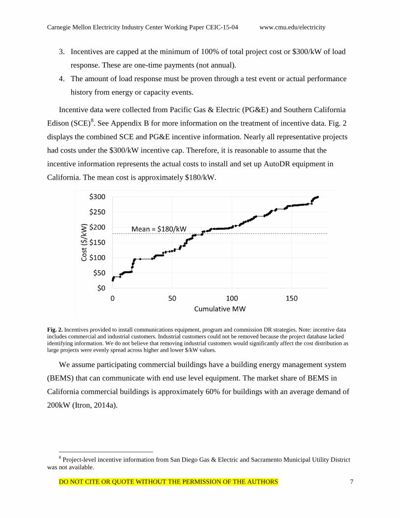
Incentive data were collected from Pacific Gas & Electric (PG&E) and Southern California

Edison (SCE)8. See Appendix B for more information on the treatment of incentive data. Fig. 2

displays the combined SCE and PG&E incentive information. Nearly all representative projects

had costs under the $300/kW incentive cap. Therefore, it is reasonable to assume that the

incentive information represents the actual costs to install and set up AutoDR equipment in

California. The mean cost is approximately $180/kW.

Fig. 2. Incentives provided to install communications equipment, program and commission DR strategies. Note: incentive data includes commercial and industrial customers. Industrial customers could not be removed because the project database lacked identifying information. We do not believe that removing industrial customers would significantly affect the cost distribution as large projects were evenly spread across higher and lower $/kW values.

We assume participating commercial buildings have a building energy management system

(BEMS) that can communicate with end use level equipment. The market share of BEMS in

California commercial buildings is approximately 60% for buildings with an average demand of

200kW (Itron, 2014a).

8 Project-level incentive information from San Diego Gas & Electric and Sacramento Municipal Utility District

was not available.



2.1.2 Telemetry

Due to the short timescales on which ancillary services operate, resources participating in

these markets are required to have telemetry. Telemetry allows the grid operator to obtain real-

time information on load characteristics, such as real and reactive power. Energy and capacity

DR programs do not rely on telemetry for measurement and verification of load reductions –

they use interval meter data that are already captured for billing purposes.

For small distributed resources like DR, the cost of telemetry is a significant obstacle to

participation in ancillary service markets. Estimates of the cost of telemetry for a large

commercial building are approximately $50,000-$80,000 (Kiliccote et al., 2014). Given the

average load response in the AutoDR program, this cost would translate to over $200/kW.

However, new designs could provide telemetry at much lower cost. Early tests show large

commercial buildings could be outfitted with telemetry at an approximate cost of $50/kW of

controlled load (Kiliccote et al., 2014). We use the $50/kW estimate for our analysis.

2.1.3 Customer Incentives

In order for an aggregator to attract DR resources, it must compensate facilities for the

possibility of interrupting their load. There are no regulated utility-based spinning reserve

programs in the United States that allow us to understand necessary customer incentives, but the

incentives provided to energy and capacity program participants can act as a guide. They may

indicate an upper bound on the incentives required for spinning reserve because reserve events

are called less often and for shorter periods of time. In SCE’s energy DR program customers

receive approximately $25/kW per year, assuming 50 hours of events. In our analysis we use an

incentive of $20/kW but consider incentives from $10/kW to $30/kW. We assume businesses

installing automated DR equipment would be willing to participate for the incentive but

acknowledge that the use of a flat customer incentive masks the differences in willingness to

participate across business and load types.

2.2 Potential Revenue Across End Uses, Business Segments, and Geographic Location

To calculate potential revenue, we gathered hourly commercial load that had been

standardized to typical weather conditions and disaggregated by geographic zone, business

segment, and end use. Using models of these profiles, we created new profiles specifically for



the period 2011-2013. Normalized hourly profiles were then matched with hourly market

clearing prices to calculate potential revenue.

By using normalized load profiles to represent DR resource availability, we assume that DR

resource availability for reserves is proportional to the load of that particular end use at that

particular time. For energy or capacity events, which can last from 1 to 8 hours in California

(SCE, 2014), this may not be an appropriate assumption. Commercial customers may not want a

portion of their electrical service interrupted for that period of time due to operational

constraints. However, spinning reserve events typically last for only 10-20 minutes, and thus

customers can shed larger percentages of their load without suffering major interruptions to

business operations. Data from PJM, the only region to publish hourly market clearing resource

amounts for DR in spinning reserve, support this assumption (see Appendix A for discussion of

this topic).

2.2.1 Load Disaggregation

One of the only large scale studies to quantify end use level demand across a broad

geographic area is the 2006 California Commercial End Use Survey (CEUS) (Itron, 2006). The

CEUS collected metered data from a stratified sample of approximately 2,700 buildings in order

to create hourly end use level load profiles. The sample was stratified across 12 geographic zones

(Fig. 3) and 12 building segments (Table 2). For each building in the survey, a simulation model

that disaggregates whole-facility load into 13 end uses (Table 2) was built in a DOE-2.2 energy

simulation environment. Simulation results were calibrated to actual consumption and weather

data to ensure the model was accurate. Once calibrated, the building model was run on a new

standardized weather set meant to represent a typical weather year in California. Buildings

within each sample strata were aggregated to produce weighted average hourly profiles. 1,872

unique hourly profiles were created across all geographic zones, building segments, and end

uses.



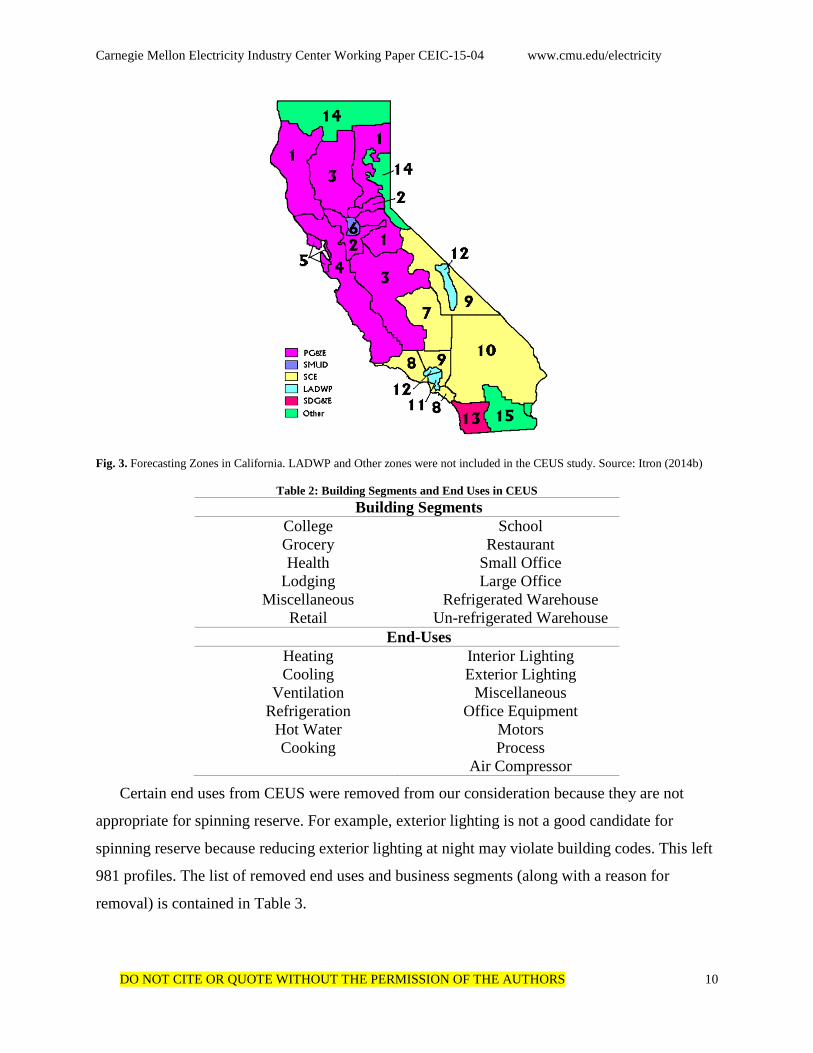
Fig. 3. Forecasting Zones in California. LADWP and Other zones were not included in the CEUS study. Source: Itron (2014b)

Table 2: Building Segments and End Uses in CEUS Building Segments

College School Grocery Restaurant Health Small Office

Lodging Large Office Miscellaneous Refrigerated Warehouse

Retail Un-refrigerated Warehouse End-Uses

Heating Interior Lighting Cooling Exterior Lighting

Ventilation Miscellaneous Refrigeration Office Equipment

Hot Water Motors Cooking Process

Air Compressor

Certain end uses from CEUS were removed from our consideration because they are not

appropriate for spinning reserve. For example, exterior lighting is not a good candidate for

spinning reserve because reducing exterior lighting at night may violate building codes. This left

981 profiles. The list of removed end uses and business segments (along with a reason for

removal) is contained in Table 3.



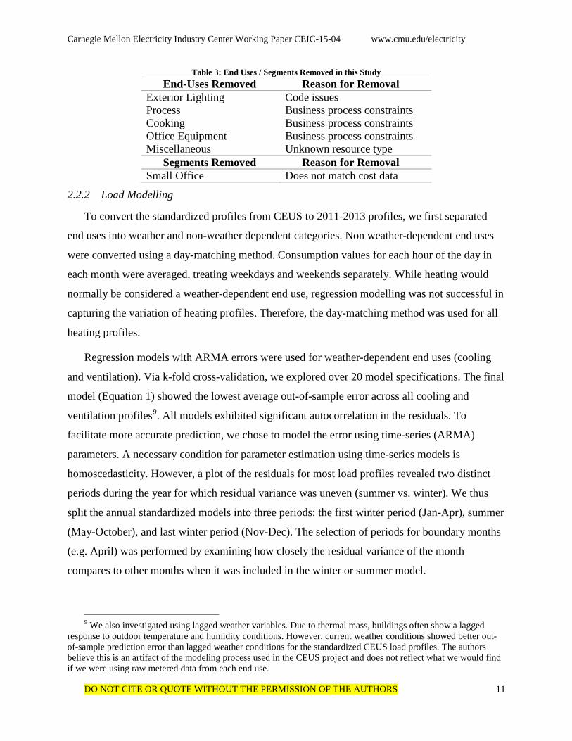
Table 3: End Uses / Segments Removed in this Study End-Uses Removed Reason for Removal

Exterior Lighting Code issues Process Business process constraints Cooking Business process constraints Office Equipment Business process constraints Miscellaneous Unknown resource type

Segments Removed Reason for Removal Small Office Does not match cost data

2.2.2 Load Modelling

To convert the standardized profiles from CEUS to 2011-2013 profiles, we first separated

end uses into weather and non-weather dependent categories. Non weather-dependent end uses

were converted using a day-matching method. Consumption values for each hour of the day in

each month were averaged, treating weekdays and weekends separately. While heating would

normally be considered a weather-dependent end use, regression modelling was not successful in

capturing the variation of heating profiles. Therefore, the day-matching method was used for all

heating profiles.

Regression models with ARMA errors were used for weather-dependent end uses (cooling

and ventilation). Via k-fold cross-validation, we explored over 20 model specifications. The final

model (Equation 1) showed the lowest average out-of-sample error across all cooling and

ventilation profiles9. All models exhibited significant autocorrelation in the residuals. To

facilitate more accurate prediction, we chose to model the error using time-series (ARMA)

parameters. A necessary condition for parameter estimation using time-series models is

homoscedasticity. However, a plot of the residuals for most load profiles revealed two distinct

periods during the year for which residual variance was uneven (summer vs. winter). We thus

split the annual standardized models into three periods: the first winter period (Jan-Apr), summer

(May-October), and last winter period (Nov-Dec). The selection of periods for boundary months

(e.g. April) was performed by examining how closely the residual variance of the month

compares to other months when it was included in the winter or summer model.

9 We also investigated using lagged weather variables. Due to thermal mass, buildings often show a lagged

response to outdoor temperature and humidity conditions. However, current weather conditions showed better out-of-sample prediction error than lagged weather conditions for the standardized CEUS load profiles. The authors believe this is an artifact of the modeling process used in the CEUS project and does not reflect what we would find if we were using raw metered data from each end use.



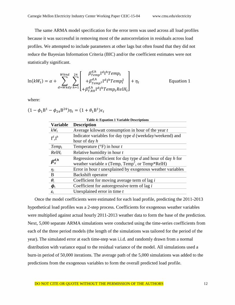
The same ARMA model specification for the error term was used across all load profiles

because it was successful in removing most of the autocorrelation in residuals across load

profiles. We attempted to include parameters at other lags but often found that they did not

reduce the Bayesian Information Criteria (BIC) and/or the coefficient estimates were not

statistically significant.

ln(𝑘𝑘𝑡) = 𝛼 + � ��

𝛽𝑇𝑇𝑇𝑇𝑑,ℎ I𝑑Iℎ𝑇𝑇𝑇𝑇𝑡

+𝛽𝑇𝑇𝑇𝑇2𝑑,ℎ I𝑑Iℎ𝑇𝑇𝑇𝑇𝑡2

+𝛽𝑇.𝑅𝑅𝑑,ℎ I𝑑Iℎ𝑇𝑇𝑇𝑇𝑡𝑅𝑇𝑅𝑅𝑡

�24

ℎ=1

+ 𝜂𝑡 Equation 1𝑊𝑊𝑊𝑑

𝑑=𝑊𝑊𝑑𝑊

where:

(1 − 𝜙1B1 − 𝜙24B24)𝜂𝑡 = (1 + 𝜃1B1)𝜖𝑡

Table 4: Equation 1 Variable Descriptions Variable Description kWt Average kilowatt consumption in hour of the year t

Id,Ih Indicator variables for day type d (weekday/weekend) and hour of day h

Tempt Temperature (°F) in hour t RelHt Relative humidity in hour t

𝜷𝒙𝒅,𝒉

Regression coefficient for day type d and hour of day h for weather variable x (Temp, Temp2, or Temp*RelH)

ηt Error in hour t unexplained by exogenous weather variables B Backshift operator θi Coefficient for moving average term of lag i 𝝓i Coefficient for autoregressive term of lag i εt Unexplained error in time t

Once the model coefficients were estimated for each load profile, predicting the 2011-2013

hypothetical load profiles was a 2-step process. Coefficients for exogenous weather variables

were multiplied against actual hourly 2011-2013 weather data to form the base of the prediction.

Next, 5,000 separate ARMA simulations were conducted using the time-series coefficients from

each of the three period models (the length of the simulations was tailored for the period of the

year). The simulated error at each time-step was i.i.d. and randomly drawn from a normal

distribution with variance equal to the residual variance of the model. All simulations used a

burn-in period of 50,000 iterations. The average path of the 5,000 simulations was added to the

predictions from the exogenous variables to form the overall predicted load profile.



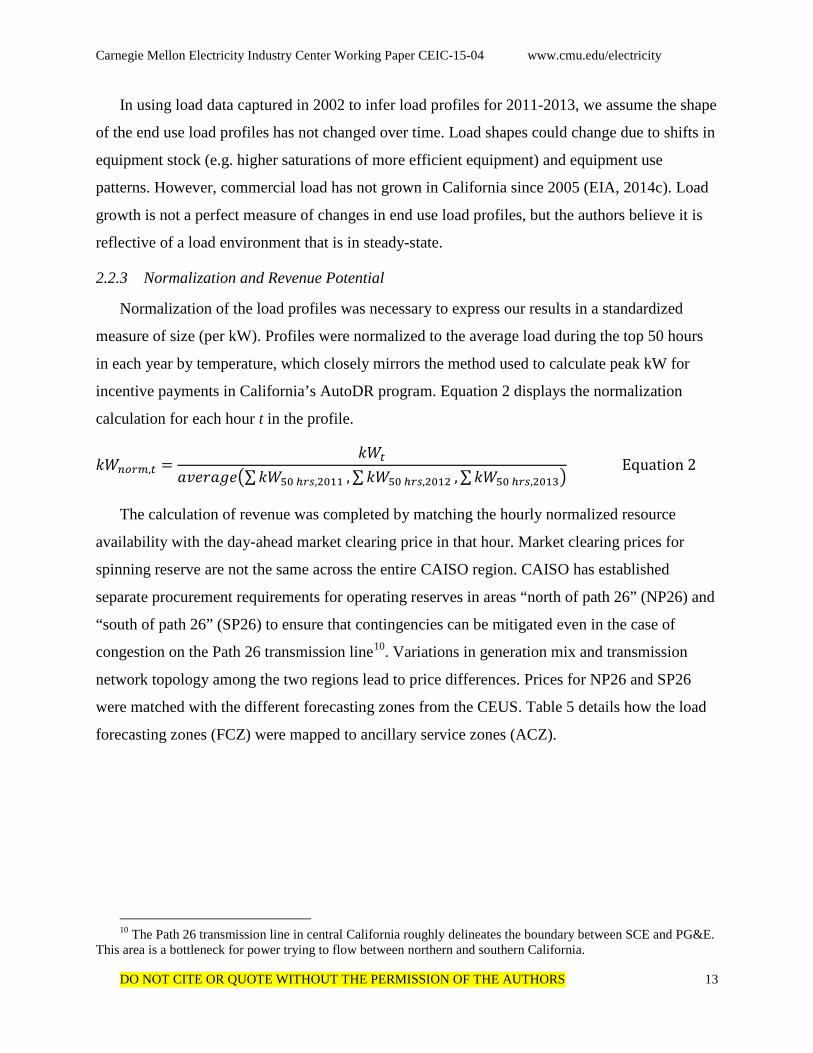
In using load data captured in 2002 to infer load profiles for 2011-2013, we assume the shape

of the end use load profiles has not changed over time. Load shapes could change due to shifts in

equipment stock (e.g. higher saturations of more efficient equipment) and equipment use

patterns. However, commercial load has not grown in California since 2005 (EIA, 2014c). Load

growth is not a perfect measure of changes in end use load profiles, but the authors believe it is

reflective of a load environment that is in steady-state.

2.2.3 Normalization and Revenue Potential

Normalization of the load profiles was necessary to express our results in a standardized

measure of size (per kW). Profiles were normalized to the average load during the top 50 hours

in each year by temperature, which closely mirrors the method used to calculate peak kW for

incentive payments in California’s AutoDR program. Equation 2 displays the normalization

calculation for each hour t in the profile.

𝑘𝑘𝑊𝑛𝑛𝑇,𝑡 =𝑘𝑘𝑡

𝑎𝑎𝑇𝑎𝑎𝑎𝑇�∑𝑘𝑘50 ℎ𝑛𝑟,2011 ,∑𝑘𝑘50 ℎ𝑛𝑟,2012 ,∑𝑘𝑘50 ℎ𝑛𝑟,2013� Equation 2

The calculation of revenue was completed by matching the hourly normalized resource

availability with the day-ahead market clearing price in that hour. Market clearing prices for

spinning reserve are not the same across the entire CAISO region. CAISO has established

separate procurement requirements for operating reserves in areas “north of path 26” (NP26) and

“south of path 26” (SP26) to ensure that contingencies can be mitigated even in the case of

congestion on the Path 26 transmission line10. Variations in generation mix and transmission

network topology among the two regions lead to price differences. Prices for NP26 and SP26

were matched with the different forecasting zones from the CEUS. Table 5 details how the load

forecasting zones (FCZ) were mapped to ancillary service zones (ACZ).

10 The Path 26 transmission line in central California roughly delineates the boundary between SCE and PG&E.

This area is a bottleneck for power trying to flow between northern and southern California.



Table 5: Forecasting Zone Mapping to Ancillary Service Zone Partitions FCZ in

Service Zone “CAISO” FCZ in

Service Zone “SP26” FCZ 1 FCZ 7

2 8 3 9 4 10 5 13 6

In making this calculation we assume perfect forecasting of resource availability, which

would tend to increase our revenue numbers. However, this did not affect the final conclusions

of the study. We also assume that load resources are price-takers that do not affect the market

clearing price. While ancillary service participants are worried that markets will saturate quickly

and prices will collapse (DOE, 2011a), as long as some traditional generation remains in the

spinning reserve market prices may not decrease significantly due to the payment of lost

opportunity costs of energy production (Cappers et al., 2013).

3. Results and Discussion

We find end uses that are relatively constant throughout the year, such as lighting or

refrigeration, are better suited for spinning reserve than seasonal end uses like cooling and

heating. This is counter to the intuition behind traditional capacity-based demand response

programs that focus on seasonal end uses because they are highly correlated with the system

peak demand. Spinning reserve, however, is needed at all times and is therefore best served by

resources which are available at all times. Fig. 4 shows the results by end use and building

segment combinations across all of the forecasting zones.



Fig. 4. Average annual revenue for end use / building segment combinations. The area of the dot represents the total peak load for that combination across all forecasting zones. The color of the dot corresponds to the average annual revenue potential. Average annual revenue is calculated as a weighted average across all zones, weighted by peak load.

While cooling is the largest end use by peak load in California, it nevertheless has very low

revenue potential because of its seasonal nature. Interior lighting is a large end use and is well

suited for spinning reserve, especially in building segments that operate on continuous schedules

such as lodging. The school and college segments which have lower seasonal loads during

capacity strained periods do especially poorly.

To determine the payback periods experienced by an aggregator participating in this market,

we compare annual revenue to costs. In Fig. 5 we fix costs at $230/kW, which includes the mean

cost of installation and the cost of telemetry but does not include customer incentives (customer

incentives are introduced in Fig. 6). We find that median payback periods are in the range of 5-

10 years and hence represent a limited profit opportunity for an aggregator.



Fig. 5. Average annual revenue and years until payback at a fixed cost of $230/kW (excludes customer incentives). Each zone-segment combination represents a single point within each end use distribution. The heavy horizontal line in the middle of each box marks the median. The range of the box represents the interquartile range. The whiskers extend to the extremes of the distribution.

We do not find important differences in revenue potential across geographic zones. The

largest driver of difference across zones is the market price for spinning reserve – southern

California often has higher prices than northern California.

However, niche applications of DR for spinning reserve can make a profit. In Fig. 6, we fix

revenue at the 75th percentile of the distribution of revenue for interior lighting, ventilation, and

refrigeration. The plots shows the cumulative percentage of projects versus payback period under

uncertainty in the cost of communication equipment installation (as given in Fig. 2). The costs

included in Fig. 6 are the costs of equipment installation, telemetry, and a $20/kW customer

incentive.



Fig. 6. Payback distribution for three end uses with fixed revenue (75th percentile of zone-segment combinations) and uncertainty in the cost of communication equipment installation and programming. Approximately 10% of projects in these end uses at the 75th percentile of revenue would have payback periods less than 5 years.

Approximately 10% of projects in the 75th percentile zone-segment combination for each of

these end uses could achieve a payback less than 5 years. The 5 year simple payback threshold is

important because many companies use simple payback as a metric for energy decisions and

most of these companies use a threshold of 5 years or less (Prindle and Fontaine, 2009). The

spinning reserve requirement in CAISO is around 3% of load (FERC 2013). Thus, a small

number of projects could have a significant effect on the mix of resources in the spinning reserve

market. Table 6 displays a sensitivity analysis of the cumulative probability of a payback less

than 5 years under different end uses and customer incentives.

Table 6: Cumulative percentage of projects with payback period less than 5 years at 75th percentile revenue. Customer Incentive $10/kW $20/kW $30/kW Refrigeration 27% 15% 7% Int. Lighting 19% 10% 0% Ventilation 16% 9% 0%

4. Conclusion and Policy Implications

4.1 Avoided Carbon Emissions



We have shown that the profitability of using DR for spinning reserve alone is inadequate to

attract interest from most DR aggregators. However, providing incentives to DR would

encourage participation. We now consider if such an incentive is justified by a market failure not

currently captured in spinning reserve clearing prices; namely, the damages associated with

carbon dioxide (CO2) emissions from fossil fuel power generation. California already considers

the social cost of carbon in their cost effectiveness tests for utility energy efficiency and demand

response programs (CPUC 2010).

To our knowledge, there has been no detailed study of the emissions avoided from DR

participation in electricity markets for either energy or ancillary services. Studies of avoided

emissions in reserve markets have mostly focused on renewable energy (Fripp, 2011) or pumped

hydroelectric power (Koritarov et al., 2014). The most rigorous approach to this problem would

make use of a dispatch model of the California grid to understand the quantity and type of fossil

fuel power plants offset from DR and the duration of offset. Here we instead make a first-order

estimate.

The procurement of spinning reserve is fundamentally an option to produce power, not an

actual call for power. Marginal changes in the fuel mix of reserves that do not change the overall

energy dispatch will not displace emissions as nothing has physically changed on the grid.

However, if enough DR is procured to offset the reserve provided by an entire plant, that plant

can shut down11. The emissions saved would be the difference between the reduction from

turning off the partly-loaded reserve plant and the increase of the base load plant that is now

making up for the energy generation of the reserve plant.

To calculate emissions savings, it is thus important to understand the fuel types which

typically provide spinning reserve and base load. The 2013 CAISO Annual Report on Market

Issues and Performance (CAISO, 2013) reports that hydro supplies approximately half of the

spinning reserve in a typical year. Natural gas and imports supply approximately a quarter of this

reserve each. Droughts and changing climate patterns, however, may reduce the potential for

high-elevation hydropower production in California in the future (Phinney and McCann, 2005).

11 This assumes that the marginal plant used for reserves is online only because of the need to provide reserve.

We adjust for this assumption in our calculations.



Reduced hydropower energy production is typically offset by natural gas in California (EIA,

2014b). We assume that reduced spinning reserve from hydropower is also offset by natural gas.

Natural gas plants represent the majority of the available dispatchable generation in CAISO,

hence the energy production from plants providing reserve that are offset by DR is likely

assumed by other natural gas generation. We assume that all natural gas generation is performed

by combined-cycle (NGCC) plants12. In this analysis, we focus just on the emissions and

associated damages from CO2 and not from criteria pollutants (e.g., sulfur dioxide, nitrogen

oxide, particulate matter)13. Social damages from CO2 are orders of magnitude larger than

damages from criteria pollutants for natural gas plants14.

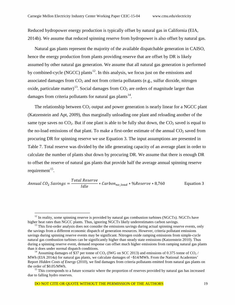
The relationship between CO2 output and power generation is nearly linear for a NGCC plant

(Katzenstein and Apt, 2009), thus marginally unloading one plant and reloading another of the

same type saves no CO2. But if one plant is able to be fully shut down, the CO2 saved is equal to

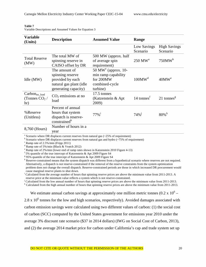
the no-load emissions of that plant. To make a first-order estimate of the annual CO2 saved from

procuring DR for spinning reserve we use Equation 3. The input assumptions are presented in

Table 7. Total reserve was divided by the idle generating capacity of an average plant in order to

calculate the number of plants shut down by procuring DR. We assume that there is enough DR

to offset the reserve of natural gas plants that provide half the average annual spinning reserve

requirement15.

𝐴𝐴𝐴𝐴𝑎𝑅 𝐶𝐶2 𝑆𝑎𝑎𝑆𝐴𝑎𝑆 =𝑇𝑇𝑇𝑎𝑅 𝑅𝑇𝑆𝑇𝑎𝑎𝑇

𝐼𝐼𝑅𝑇∗ 𝐶𝑎𝑎𝐶𝑇𝐴𝑊𝑛_𝑙𝑛𝑙𝑑 ∗ %𝑅𝑇𝑆𝑇𝑎𝑎𝑇 ∗ 8,760 Equation 3

12 In reality, some spinning reserve is provided by natural gas combustion turbines (NGCTs). NGCTs have

higher heat rates than NGCC plants. Thus, ignoring NGCTs likely underestimates carbon savings. 13 This first-order analysis does not consider the emissions savings during actual spinning reserve events, only

the savings from a different economic dispatch of generation resources. However, criteria pollutant emissions savings during spinning reserve events may be significant. Nitrogen oxide ramping emissions from simple-cycle natural gas combustion turbines can be significantly higher than steady state emissions (Katzenstein 2010). Thus during a spinning reserve event, demand response can offset much higher emissions from ramping natural gas plants than it does under normal dispatch conditions.

14 Assuming damages of $37 per tonne of CO2 (IWG on SCC 2013) and emissions of 0.375 tonne of CO2 / MWh (EIA 2014a) for natural gas plants, we calculate damages of ~$14/MWh. From the National Academies’ Report Hidden Costs of Energy (2010), we find damages from criteria pollutants emitted from natural gas plants on the order of $0.05/MWh.

15 This corresponds to a future scenario where the proportion of reserves provided by natural gas has increased due to falling hydro reserves.



Table 7 Variable Descriptions and Assumed Values for Equation 3

Variable (Units) Description Assumed Value Range

Low Savings Scenario

High Savings Scenario

Total Reserve (MW)

The total MW of spinning reserve in CAISO offset by DR

500 MW (approx. half of average spin requirement)

250 MWa 750MWb

Idle (MW)

The amount of spinning reserve provided by each natural gas plant (idle generating capacity)

50 MWc (approx. 10-min ramp capability for 200MW combined-cycle turbine)

100MWd 40MWe

Carbonno_load (Tonnes CO2 / hr)

CO2 emissions at no load

17.5 tonnes (Katzenstein & Apt 2009)

14 tonnesf 21 tonnesg

%Reserve (Unitless)

Percent of annual hours that system dispatch is reserve-constrainedh

77%i 74%j 80%k

8,760 (Hours) Number of hours in a year

a Scenario where DR displaces current reserves from natural gas (~25% of requirement) b Scenario where DR displaces current reserves from natural gas and hydro (~75% of requirement) c Ramp rate of 2.5%/min (Fripp 2011) d Ramp rate of 5%/min (Black & Veatch 2012) e Ramp rate of 2%/min (lower end of ramp rates shown in Katzenstein 2010 Figure 4-13) f 5% quantile of the true intercept of Katzenstein & Apt 2009 Figure S4 g 95% quantile of the true intercept of Katzenstein & Apt 2009 Figure S4 h Reserve-constrained means that the system dispatch was different from a hypothetical scenario where reserves are not required.

Alternatively, a dispatch is not reserve-constrained if the removal of the reserve constraints from the system optimization problem does not change the overall dispatch. Reserve-constrained periods are those in which increased DR procurement would cause marginal reserve plants to shut down.

i Calculated from the average number of hours that spinning reserve prices are above the minimum value from 2011-2013. A reserve price at the minimum value reflects a system which is not reserve-constrained.

j Calculated from the low annual number of hours that spinning reserve prices are above the minimum value from 2011-2013. k Calculated from the high annual number of hours that spinning reserve prices are above the minimum value from 2011-2013.

We estimate annual carbon savings at approximately one million metric tonnes (0.2 x 106 –

2.8 x 106 tonnes for the low and high scenarios, respectively). Avoided damages associated with

carbon emission savings were calculated using two different values of carbon: (1) the social cost

of carbon (SCC) computed by the United States government for emissions year 2010 under the

average 3% discount rate scenario ($37 in 2014 dollars) (IWG on Social Cost of Carbon, 2013),

and (2) the average 2014 market price for carbon under California’s cap and trade system set up



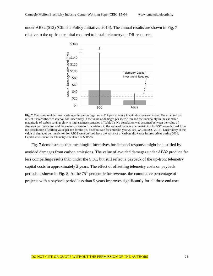
under AB32 ($12) (Climate Policy Initiative, 2014). The annual results are shown in Fig. 7

relative to the up-front capital required to install telemetry on DR resources.

Fig. 7. Damages avoided from carbon emission savings due to DR procurement in spinning reserve market. Uncertainty bars reflect 90% confidence interval for uncertainty in the value of damages per metric ton and the uncertainty in the estimated magnitude of carbon savings (low to high savings scenarios of Table 7). No correlation was assumed between the value of damages per metric ton and the savings scenario. Uncertainty in the value of damages per metric ton for SSC were derived from the distribution of carbon value per ton for the 3% discount rate for emission year 2010 (IWG on SCC 2013). Uncertainty in the value of damages per metric ton for AB32 were derived from the variance of carbon allowance futures prices during 2014. Capital investment for telemetry calculated at $50/kW.

Fig. 7 demonstrates that meaningful incentives for demand response might be justified by

avoided damages from carbon emissions. The value of avoided damages under AB32 produce far

less compelling results than under the SCC, but still reflect a payback of the up-front telemetry

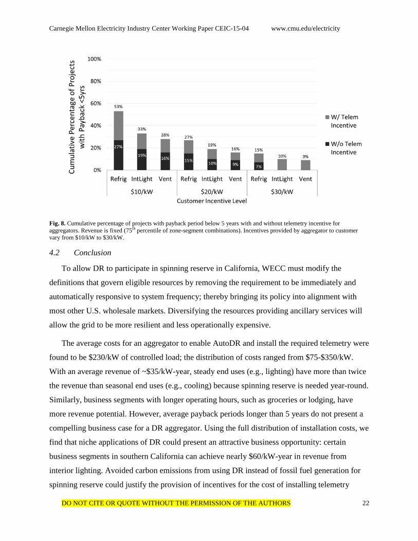
capital costs in approximately 2 years. The effect of offsetting telemetry costs on payback

periods is shown in Fig. 8. At the 75th percentile for revenue, the cumulative percentage of

projects with a payback period less than 5 years improves significantly for all three end uses.



Fig. 8. Cumulative percentage of projects with payback period below 5 years with and without telemetry incentive for aggregators. Revenue is fixed (75th percentile of zone-segment combinations). Incentives provided by aggregator to customer vary from $10/kW to $30/kW.

4.2 Conclusion

To allow DR to participate in spinning reserve in California, WECC must modify the

definitions that govern eligible resources by removing the requirement to be immediately and

automatically responsive to system frequency; thereby bringing its policy into alignment with

most other U.S. wholesale markets. Diversifying the resources providing ancillary services will

allow the grid to be more resilient and less operationally expensive.

The average costs for an aggregator to enable AutoDR and install the required telemetry were

found to be $230/kW of controlled load; the distribution of costs ranged from $75-$350/kW.

With an average revenue of ~$35/kW-year, steady end uses (e.g., lighting) have more than twice

the revenue than seasonal end uses (e.g., cooling) because spinning reserve is needed year-round.

Similarly, business segments with longer operating hours, such as groceries or lodging, have

more revenue potential. However, average payback periods longer than 5 years do not present a

compelling business case for a DR aggregator. Using the full distribution of installation costs, we

find that niche applications of DR could present an attractive business opportunity: certain

business segments in southern California can achieve nearly $60/kW-year in revenue from

interior lighting. Avoided carbon emissions from using DR instead of fossil fuel generation for

spinning reserve could justify the provision of incentives for the cost of installing telemetry



(~$50/kW) for DR resources. Avoided emissions may be larger in regions with higher

proportions of coal-fired resources.

Acknowledgements

This work was supported by grants from the Richard King Mellon Foundation and the

Electric Power Research Institute. Neither funding source had any role in study design,

collection, analysis and interpretation of data, writing of the paper, or in the decision to submit

the article for publication. We thank Ines Azevedo, Alex Davis, Roger Lueken, Stephen Rose

and Kyle Siler-Evans of Carnegie Mellon University for helpful comments and suggestions. We

also thank Girish Ghatikar of Lawrence Berkeley National Laboratory for providing background

and incentive information related to the AutoDR program, as well as Daniel Olsen of Lawrence

Berkeley National Laboratory and Mark Ciminelli of the California Energy Commission for their

help in deciphering the CEUS data and results.

References

145 FERC ¶ 61,141 (2013). Regional Reliability Standard BAL-002-WECC-2 – Contingency Reserve, Order No. 789.

CAISO, 2010. Sub-Regional Partition FAQ. Available at: http://www.caiso.com/Documents/ScarcityPricingPartitionFAQ.pdf. Accessed October 2014.

CAISO, 2013. 2013 Annual Report on Market Issues & Performance. Department of Market Monitoring. Available at: http://www.caiso.com/Documents/2013AnnualReport-MarketIssue-Performance.pdf. Accessed September 2014.

CAISO 2014. Business Practice Manual for Market Operations. Version 40, last revised 7/9/2014. Available at: http://www.caiso.com/rules/Pages/BusinessPracticeManuals/Default.aspx. Accessed October, 2014.

California Public Utilities Commission, 2010. Demand Response Cost Effectiveness Protocols. R.07-01-041.

Callaway, D.S., 2009. Tapping the energy storage potential in electric loads to deliver load following and regulation, with application to wind energy. Energy Conversion and Management, 50(5), pp.1389–1400.

Callaway, D.S., Hiskens, I. a, 2011. Achieving Controllability of Electric Loads. Proceedings of the IEEE, 99(1), pp.184–199.

http://www.caiso.com/Documents/ScarcityPricingPartitionFAQ.pdf

http://www.caiso.com/Documents/2013AnnualReport-MarketIssue-Performance.pdf

http://www.caiso.com/Documents/2013AnnualReport-MarketIssue-Performance.pdf

http://www.caiso.com/rules/Pages/BusinessPracticeManuals/Default.aspx



Cappers, P., Macdonald, J., Goldman, C., 2013. Market and Policy Barriers for Demand Response Providing Ancillary Services in U.S. Electricity Markets. Lawrence Berkeley National Laboratory. LBNL-6155E.

Climate Policy Initiative, 2014. California Carbon Dashboard. Available at: http://calcarbondash.org/. Accessed November 24, 2014.

Ela, E., Milligan, M., Kirby, B., 2011. Operating Reserves and Variable Generation. National Renewable Energy Laboratory. NREL/TP-5500-51978.

Ellison, J.F., Tesfatsion, L.S., Loose, V.W., Byrne, R.H., 2012. Project Report: A Survey of Operating Reserve Markets in U.S. ISO/RTO-managed Electric Energy Regions. Sandia National Laboratories. SAND2012-1000.

Eto, J.H., Nelson-Hoffman, J., Parker, E., Bernier, C., Young, P., Sheehan, D., Kueck, J., Kirby, B., 2007. Demand Response Spinning Reserve Demonstration. Lawrence Berkeley National Laboratory. LBNL-62761.

Fripp, M., 2011. Greenhouse gas emissions from operating reserves used to backup large-scale wind power. Env. Sci. & Tech., 45(21), pp.9405–12.

Ghatikar, G., Riess, D., Piette, M.A., 2014. Analysis of Open Automated Demand Response Deployments in California and Guidelines to Transition to Industry Standards. Lawrence Berkeley National Laboratory. LBNL-6560E.

Hummon, M., Denholm, P., Jorgenson, J., Palchak, D., Kirby, B., Ma, O., 2013. Fundamental Drivers of the Cost and Price of Operating Reserves. National Renewable Energy Laboratory. NREL/TP-6A20-58491.

Hummon, M., Palchak, D., Denholm, P., Jorgenson, J., Olsen, D., Kiliccote, S., Matson, N., Sohn, M., Rose, C., Dudley, J., Goli, S., Ma, O., 2013. Grid Integration of Aggregated Demand Response, Part 2: Modeling Demand Response in a Production Cost Model. National Renewable Energy Laboratory. NREL/TP-6A20-58492.

Interagency Working Group on Social Cost of Carbon, 2013 Technical Support Document: Technical Update of the Social Cost of Carbon for Regulatory Impact Analysis Under Executive Order 12866 (US Government, Washington, DC). Revised November 2013.

Itron, 2006. California Commercial End Use Survey. Prepared for the California Energy Commission. CEC-400-2006-005.

Itron, 2014a. California Commercial Saturation Survey. Prepared for the California Energy Commission. Available at: http://calmac.org/publications/California_Commercial_Saturation_Study_Report_Finalv2.pdf. Accessed October 2014.

Itron, 2014b. California Energy Commission Forecasting Climate Zone Map. http://capabilities.itron.com/CeusWeb/FCZMap.aspx. Accessed May 2014.

Katzenstein, W., 2010. Wind Power Variability, Its Cost, and Effect on Power Plant Emissions. Dissertation submitted for Doctor of Philosophy. July 2010. Carnegie Mellon University.

Katzenstein, W., Apt, J., 2009. Response to Comment on “Air Emissions Due to Wind and Solar Power.” Env. Sci. & Tech., 43(15), pp.6108–6109.

http://calcarbondash.org/

http://calmac.org/publications/California_Commercial_Saturation_Study_Report_Finalv2.pdf

http://calmac.org/publications/California_Commercial_Saturation_Study_Report_Finalv2.pdf

http://capabilities.itron.com/CeusWeb/FCZMap.aspx



Kiliccote, S., Lanzisera, S., Liao, A., Schetrit, O., Piette, M.A., 2014. Fast DR: Controlling Small Loads over the Internet. In 2014 ACEEE Summer Study on Energy Efficiency in Buildings. pp. 196–208.

Kirby, B., 2003. Spinning Reserve From Responsive Loads. Oak Ridge National Laboratory. ORNL/TM-2003/19.

Koritarov, V., Veselka, T., Gasper, J., Bethke, B., Botterud, A., Wang, J., Mahalik, M., Zhou, Z., Milostan, C., Feltes, J., Kazachkov, Y., Guo, T., Liu, G., Trouille, B., Donalek, P., King, K., Ela, E., Kirby, B., Krad, I., Gevorgian, V., 2014. Modeling and Analysis of Value of Advanced Pumped Storage Hydropower in the United States. Argonne National Laboratory. ANL/DIS-14/7.

Lueken, R., 2014. Reducing Carbon Intensity in Restructured Markets: Challenges and Potential Solutions. Dissertation submitted for Doctor of Philosophy. September 2014. Carnegie Mellon University.

Ma, O., Alkadi, N., Cappers, P., Denholm, P., Dudley, J., Goli, S., Hummon, M., Kiliccote, S., Macdonald, J., Matson, N., Olsen, D., Rose, C., Sohn, M.D., Starke, M., Kirby, B., O'Malley, M., 2013. Demand Response for Ancillary Services. IEEE Transactions on Smart Grid, 4(4), pp.1988–1995.

Macdonald, J., Cappers, P., Callaway, D., Kiliccote, S., 2012. Demand Response Providing Ancillary Services. Presented at Grid-Interop Forum 2012. Irving, TX. LBNL-5958E. Available at: http://drrc.lbl.gov/sites/all/files/LBNL-5958E.pdf. Accessed March 2014.

Macdonald, J., Kiliccote, S., Berkeley, L., 2014. Commercial Building Loads Providing Ancillary Services in PJM. In 2014 ACEEE Summer Study on Energy Efficiency in Buildings. pp. 192–206.

Mathieu, J.L., Dyson, M., Callaway, D.S., 2012. Using Residential Electric Loads for Fast Demand Response: The Potential Resource and Revenues, the Costs, and Policy Recommendations. In ACEEE Summer Study on Energy Efficiency in Buildings. pp. 189–203.

National Research Council, 2010. Hidden Costs of Energy: Unpriced Consequences of Energy Production and Use. (National Academy, Washington, DC).

NERC, 2011. Balancing and Frequency Control: A Technical Document Prepared by the NERC Resources Subcommittee. Available at: http://www.nerc.com/docs/oc/rs/NERC%20Balancing%20and%20Frequency%20Control%20040520111.pdf. Accessed April 2014.

Olsen, D.J., Matson, N., Sohn, M., Rose, C., Dudley, J., Goli, S., Kiliccote, S., Hummon, M., Palchak, D., Denholm, P., Jorgenson, J., Ma, O., 2013. Grid Integration of Aggregated Demand Response, Part I: Load Availability Profiles and Constraints for the Western Interconnection. Lawrence Berkeley National Laboratory. LBNL-6417E.

OpenADR Alliance, 2014. The OpenADR Primer: An Introduction to Automated Demand Response and the OpenADR Standard. Available at: http://www.openadr.org/assets/docs/openadr_primer.pdf. Accessed August 2014.

http://drrc.lbl.gov/sites/all/files/LBNL-5958E.pdf

http://www.nerc.com/docs/oc/rs/NERC%20Balancing%20and%20Frequency%20Control%20040520111.pdf

http://www.nerc.com/docs/oc/rs/NERC%20Balancing%20and%20Frequency%20Control%20040520111.pdf

http://www.openadr.org/assets/docs/openadr_primer.pdf



PG&E, 2009. 2009 Pacific Gas and Electric Company Participating Load Pilot Evaluation. Available at: http://www.pge.com/includes/docs/pdfs/mybusiness/energysavingsrebates/demandresponse/cs/2009_pacific_gas_and_electric_company_large_commercial_industrial_participating_load_pilot.pdf. Accessed September 2014.

Phinney, S., McCann, R., 2005. Potential Changes in Hydropower Production From Global Climate Change in California and the Western United States. Prepared for the California Energy Commission. CEC-700-2005-010.

Prindle, W., de Fontaine, A., 2009. A Survey of Corporate Energy Efficiency Strategies. In ACEEE Summer Study on Energy Efficiency in Buildings. pp. 77–89.

Rubinstein, F., Xiaolei, L., Watson, D.S., 2010. Using Dimmable Lighting for Regulation Capacity and Non-Spinning Reserves in the Ancillary Services Market: A Feasibility Study. Lawrence Berkeley National Laboratory. LBNL-4190E.

Southern California Edison, 2014. Demand Response Event History. Available at: https://www.sce.openadr.com/dr.website/scepr-event-history.jsf. Accessed November 2014.

U.S. Energy Information Administration (EIA), 2014a. Assumptions to the Annual Energy Outlook 2014. U.S. Department of Energy: Washington, DC, June 2014.

U.S. Energy Information Administration (EIA), 2014b. California drought leads to less hydropower, increased natural gas generation. Available at: http://www.eia.gov/todayinenergy/detail.cfm?id=18271#tabs_SpotPriceSlider-1. Accessed November, 2014.

U.S. Energy Information Administration (EIA), 2014c. Electric Power Annual.

US DOE, 2006. Benefits of Demand Response in Electricity Markets and Recommendations for Achieving Them. A Report to Congress in fulfillment of Sec. 1252(e) of the Energy Policy Act of 2005.

US DOE, 2011a. Load Participation in Ancillary Services: Workshop Report. Available at: https://www1.eere.energy.gov/analysis/pdfs/load_participation_in_ancillary_services_workshop_report.pdf. Accessed February 2014.

US DOE, 2011b. Recovery Act Selections for Smart Grid Investment Grant Awards – By Category. Available at: http://www.energy.gov/sites/prod/files/SGIG%20Awards%20by%20Category%202011%2011%2015.pdf. Accessed September 15, 2014.

Watson, D.S., Matson, N., Page, J., Kiliccote, S., Piette, M.A., Corfee, K., Seto, B., Masiello, R., Masiello, J., Molander, L., Golding, S., Sullivan, K., Johnson, W., Hawkings, D., 2012. Fast Automated Demand Response to Enable the Integration of Renewable Resources. Lawrence Berkeley National Laboratory. LBNL-5555E.

http://www.pge.com/includes/docs/pdfs/mybusiness/energysavingsrebates/demandresponse/cs/2009_pacific_gas_and_electric_company_large_commercial_industrial_participating_load_pilot.pdf



https://www.sce.openadr.com/dr.website/scepr-event-history.jsf

http://www.eia.gov/todayinenergy/detail.cfm?id=18271#tabs_SpotPriceSlider-1

https://www1.eere.energy.gov/analysis/pdfs/load_participation_in_ancillary_services_workshop_report.pdf

https://www1.eere.energy.gov/analysis/pdfs/load_participation_in_ancillary_services_workshop_report.pdf

http://www.energy.gov/sites/prod/files/SGIG%20Awards%20by%20Category%202011%2011%2015.pdf

http://www.energy.gov/sites/prod/files/SGIG%20Awards%20by%20Category%202011%2011%2015.pdf


DO NOT CITE OR QUOTE WITHOUT THE PERMISSION OF THE AUTHORS B-1

Appendix A DR availability proportional to load

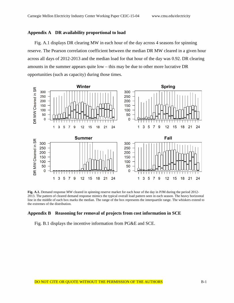
Fig. A.1 displays DR clearing MW in each hour of the day across 4 seasons for spinning

reserve. The Pearson correlation coefficient between the median DR MW cleared in a given hour

across all days of 2012-2013 and the median load for that hour of the day was 0.92. DR clearing

amounts in the summer appears quite low – this may be due to other more lucrative DR

opportunities (such as capacity) during those times.

Fig. A.1. Demand response MW cleared in spinning reserve market for each hour of the day in PJM during the period 2012-2013. The pattern of cleared demand response mimics the typical overall load pattern seen in each season. The heavy horizontal line in the middle of each box marks the median. The range of the box represents the interquartile range. The whiskers extend to the extremes of the distribution.

Appendix B Reasoning for removal of projects from cost information in SCE

Fig. B.1 displays the incentive information from PG&E and SCE.



Fig. B.1. (a) Incentives Provided by PG&E for AutoDR. (b) Incentives Provided by SCE for AutoDR.

The authors conducted an investigation into the AutoDR program costs and found that nearly

all of the projects which had incentives of $300/kW in the SCE territory were likely from one

contractor that received money from the American Recovery and Reinvestment Act (ARRA)

grant funds. We surmise that the use of ARRA funds may have led to different recruitment

practices and cost reporting. Thus, we do not believe that the incentive information reported for

these projects is representative of the rest of the project population. The list below provides

details on why the authors believe that these projects were from one contractor.

• An AutoDR program report stated that “the U.S Department of Energy’s $11.4 million

American Recovery and Reinvestment Act grant influenced a larger load shed and

enablement cost in the SCE territory.” (Ghatikar et al. 2014)

• ARRA records show a total AutoDR project cost of $22.8M in SCE (US DOE 2011b)

attributable to one company. The 50% cost sharing required by ARRA leads to a grant of

$11.4 million.

• There are 348 facilities in the project incentive database from SCE that had project

incentives of $300/kW. These projects have a total load response of 67MW. The total

rebate amount given to these participants was just over $20M, which closely matches the

ARRA project cost report.

We believe that most, if not all of the projects with incentive values at $300/kW were not

representative of the true costs to install, program, and commission this equipment. This is

especially apparent when you compare the incentive distribution from SCE with that of PG&E.



There may be other projects in the database with incentive costs of less than $300/kW that were

implemented by this DR contractor. However, we have no way of differentiating those projects.