The Economic Effects of Minimum Wage Policy

Yu Benjamin Fu∗

Simon Fraser University

Abstract

In spite of their positive influence on living standards and social inequality, it is commonly agreed

that minimum wage laws reduce output because they produce unemployment. This paper suggests that

minimum wage policy may be beneficial for a transitional economy in which labor is migrating from rural

areas to urban areas when positive moving costs occur. With a moving cost wedge a modestly binding

minimum wage can cause relatively low productivity urban workers to be replaced by higher productivity

rural migrants, and therefore increase aggregate output. Moreover, minimum wage policy can be used to

affect migration flows and social inequality. To show this, I first construct a structual model of migration,

and then simulate the calibrated model by using data from China. The results suggest that minimum

wage policy may benefit the whole economy if it is only binding for urban workers but not for migrant

workers in the urban industrial sector. Otherwise output is negatively affected. To achieve the second

best outcome, government shall fully compensate the moving costs for the marginal migrant workers who

move from the rural industrial sector to the urban subsistence sector and a binding minimum wage shall

be imposed on the urban workers but not the migrant workers in the urban industrial sector.

Key words: minimum wage, internal migration, selection, inequality, China

JEL classification codes: J61, O15, O18, O53

1 Introduction

Nowadays minimum wage policy has been popularly used in both developed and developing countries, even

though it serves different purposes. As pointed out by Watanabe (1976), developed countries intend to

use minimum wages to provide an acceptable living standard for their marginal workers, while developing

countries intend to use minimum wages to adjust their social inequalities. It is commonly agreed that

∗Department of Economics, Simon Fraser University, 8888 University Drive, Burnaby, B.C., V5A 1S6, Canada; email:yuf@sfu.ca

1

minimum wages increase unemployment and reduce output when workers are homogenous and labor markets

are perfectly competitive in the presence of perfect information. Absent these restrictive assumptions,

however, many economists draw different conclusions. For example, some have shown that minimum wages

might be Pareto optimal if the labor market is not competitive (Boal & Ransom (1997), Strobl & Walsh

(2007), and Ashenfelter, Farber & Ransom (2010) have shown that minimum wages decrease unemployment

in a monopsony market); if workers are not homogeneous (Drazen (1986) suggested that, with heterogeneous

workers, minimum wage may be Pareto optimal if a higher wage would be preferred to the market clearing

wage, even though unemployment is produced); and if there is no perfect information (Broadway & Cuff

(2001) argued that minimum wage may be optimal because it can be combined with the institutional features

of a typical welfare system to fix the government’s asymmetric information problem with respect to workers’

abilities).

In this paper, I study the effects of minimum wages on a transitional economy, such as China, in which

migration flows from rural to urban areas occur with positive moving costs. There are three main results

from my analysis. First, minimum wage is an useful instrument for the government to control migration

flows. Second, regarding social inequality adjustments, a minimum wage leads to improvements in urban

areas, but to a worsening in both rural areas and the country as a whole. Third, a minimum wage may

be optimal due to the moving friction: a moving cost wedge induces a modestly binding minimum wage to

cause relatively low productivity urban workers to be replaced by higher productivity rural migrants. To

show these results, I construct a theoretical model, focusing on the selection effects on determining the labor

market outcomes, and then compare the outcomes with minimum wages to the status quo ante. Theory

indicates that minimum wage policy has different effects on migration flows to formal sector, depending on

the level at which it is set. When its value is low, minimum wage induces fewer urban workers but more

migrant workers to work in the urban modern industrial sector. However, when its value is high, migrant

workers are also constrained from entering the urban industrial sector. The effects on the urban informal

sector are unclear. I then calibrate my theoretical model by using data from China to simulate the effects of

minimum wages. I begin by calibrating my model’s parameters to match labor market outcomes in China

in 2006. By using 2006 as benchmark, the calibrated model predicts that when the minimum wage is not

high enough to constrain qualified rural workers from moving to the urban industry sector, it benefits the

whole economy; otherwise, it has negative effects on economic growth. The calibration also predicts worse

inequality in rural areas but less inequality in urban areas, given the same investment profile. To achieve the

second best outcome, government shall fully compensate the moving costs for the marginal migrant workers

from the rural industrial sector to the urban subsistence sector, and the minimum wage shall not be binding

for migrant workers in the urban industrial sector.

2

A minimum-wage system was offi cially introduced in China’s Labor Law in 1994. It stated that the

minimum wage should be set to ensure that the lowest wage earned by a worker be suffi cient to support her

basic needs. The Labor Law was an attempt to protect workers by specifying the form of payment, maximum

hours, and overtime rates. In reality, it functioned more like a set of recommendations than binding policy,

because there was no solid punishment for firms that did not abide by it. Although the minimum wage

increased several times after 1994, the average income of low-skilled workers fell further behind the average

urban income. Between 1994 and 2004, the average annual income of civil servants in Dongguan City

increased by as much as 340%, from 8,000 RMB to more than 35,000 RMB; during the same period, average

wages in the leather and shoe industry stayed between 6,000 RMB to 10,000 RMB, and only increased by a

total of 71%.1 The Provisions on Minimum Wages was enacted in 2003 by the Ministry of Labor and Social

Security, as an attempt to strengthen the protection of low-skill workers provided by the minimum-wage

system. It required that the minimum wage be readjusted at least every two years according to such factors

as the cost of basic necessities for employees and their dependents, as well as the local consumer price index.

The readjustment was frozen in 2009 due to the worldwide recession. In 2010, following the recovery of

China’s economy and due to shortages of migrant workers, 30 of China’s 31 provinces and direct-controlled

municipalities announced increases in their minimum wages, at different rates. For example, Shanghai has

China’s highest minimum wage at 1120 RMB per month– an increase of 16.7%; in Guangdong province it

increased by 21.1%; Hainan province saw the greatest increase at 37%.2 But these wages are still very low

when compared with the local average wage. For example, the average wage in Shanghai was 3759 RMB in

2009, while its minimum wage in 2010 was only 30% of that.3

This paper analyzes the effects of minimum wage policy by using China as an example. Followed by

the introduction, the rest of this paper is organized as follows. Section 2 contains the basic model setup

and analysis. Section 3 analyzes the effects of minimum wage policy. Section 4 provides calibrations and

simulations of my model. Section 5 discusses some potential policy implications. Section 6 concludes, and

suggests some potential extensions.

2 Model Analysis

I construct a model with two regions, rural and urban, and four sectors to facilitate internal migration. Each

region has two sectors. Rural areas possess a traditional agricultural (RA) sector and a modern industrial

(RM) sector. Urban areas possess a formal urban modern industry (UM) sector and an informal urban1More information can be found in Wages in China, published on China Labor Bulletin on Feb 19th, 20082The information is published on the offi cial website of The Central People’s Government of The People’s Republic of China.3Numbers are quoted from the Shanghai Statistical Yearbook 2010.

3

subsistence (US) sector. The RM sector is developed with some exogenous physical capital investment,

which is significantly less than is invested in urban areas. The rural labor force is Lr, the urban labor force is

Lu, and I assume Lr is much greater than Lu. I also assume that each worker possesses some human capital.4

Initial levels of human capital are determined by nature, while education and job-training yield significant

increases. Each worker has his own human capital, ai, which ranges from 0 to 1. The distributions of

human capital in the rural and urban populations are pr and pu, respectively. Since education resources are

allocated more to urban areas, and since there is unequal access to post-secondary education, pu is assumed

to exhibit first-order stochastic dominance over pr.

In the RA sector, labor is considered homogeneous. The production function is:

ya = g(Na) (1)

where Na is total physical labor input. I assume g′> 0 > g

′′. Farmers are paid at their marginal products

of labor (MPNs) and the government, as the landowner, takes all the remaining output.

In the industrial sector, I assume agents work individually and the production functions are CRTS.

Workers are paid their marginal product. Each worker’s production function in UM and RM are:

yumi = f(N, ai, ku) (2)

yrmi = h(N, ai, kr) (3)

where ai is the human capital possessed by worker i, and N is the physical labor input of each worker,

which is normalized to 1. Note that I assume total capital investment in both industrial sectors is equally

distributed among the workers, ku = Ku/Lu and kr = Kr/Lr . The marginal product of labor, MPNi,

is increasing with ai and k, as capital and labor are complements. Government allocation of investment

between sectors is assumed to be exogenous, and Ku > Kr. Manufactured goods are homogeneous.

The relative price between agricultural goods and industrial goods, P, clears the market. Manufactured

goods are defined as the numeraire. The price function is:

P = ρ(yayum

) (4)

4Here human capital is defined as the stock of skill and knowledge embodied in the ability to perform labor, so it can bemeasured in terms of productivity.

4

with ρ′(·) < 0.5

2.1 The best outcomes

The first best outcome occurs when all resources are mobile across sectors, and there is thus no difference

between urban and rural areas. In the first best case, capital goes to the sector with higher returns between

industrial sector and agricultural sector. There is a boundary of human capital in that those workers

with higher human capital work in the manufacturing sector and those with lower human capital work in

the agricultural sector. Since in my model labor is the only flexible factor and there are many practical

constraints, the first best case is not possible in the real world at least in the near future, and thus it will

not be discussed in detail.

The second best outcome occurs with only one constraint: that is, capital is predetermined. In the second

best case, the difference between urban and rural areas exists since investment profiles are quite different.

To induce the second best outcome, the moving costs must be assumed away. If the US sector is assumed

to be a channel to reallocate social wealth and produce no real outputs, and the utility functions are based

on real outputs only, the second best outcome must satisfy several conditions. First, agents’utilities are

maximized given the outputs of manufactured goods and agricultural goods. Second, workers with the same

human capital are treated equally. That is, either they are all in the same sector or they are all out of that

sector, since labor is totally mobile. Third, in the second best outcome the marginal products of labor for

the same worker must be equalized across UM and RM sectors, which determines the labor allocation. This

may imply a urban-to-rural migration flow to the RM sector if it requires more workers.

Based on my model setup, the second best outcome may be derived in a simple way. Because of the

properties of the production functions in modern industry sectors, there are two opposite effects when an

extra worker enters. On the one hand, labor increases, contributing positively to total outputs. On the

other hand, the extra workers decrease the capital available to each worker, which has a negative effect on

output. Therefore the total output may be maximized at a certain cut-off level of human capital. At this

cut-off level of human capital, once the ratio between manufacturing goods and agricultural goods exceeds

the optimal ratio of subjective demands which is determined by equating the marginal utilities of consuming

each good, some workers must switch from the industrial sector to the agricultural sector until the output

ratio is optimal. Otherwise, the second-best outcome is induced. Numerical analysis cannot be done without

specific assumptions on functional forms. I discuss this further in Section 4.

5One possible way to endogenize it is to assume homogeneous preferences over both agricultural and industrial goods (e.g.Cobb-Douglas). Given a relative price level, the consumption ratio is constant and should be proportional to the ratio of outputswhen the market clears. Thus relative price is negatively related to the ratio of outputs. Please refer to Appendix A.

5

The equilibrium outcome that we may observe in the real world is the market equilibrium. Besides the

constraint imposed on the second best case, the market equilibrium also experiences positive moving costs.

This is the main focus of this paper.

2.2 The market equilibrium outcome

To determine the market equilibrium outcome, moving costs must be considered since migrant workers

are subject to them in the real world. The costs of moving to big cities are not just pecuniary, but also

include psychological discomfort, such as loneliness, discrimination from urban residents, safety issues, etc.6

Assuming high-skilled people adapt to a new environment faster, the cost of moving is modeled as a decreasing

function of ai. 7 I assume the annuitized cost of moving is C(ai) with C ′(·) < 0.8

When a rural worker considers moving, she compares the benefits of moving to the cost. By assuming

that a higher wage is the benefit she would earn if working in an urban area, her net benefit function is:

B(ai) = w(ai)− C(ai) (5)

I assume that wum(1)− C(1)− wrm(1) > 0, i.e.

f ′N (1,Ku/Lu

∫ 1

au

pudar)− C(1)− h′N (1,Kr/Lr

∫ 1

ar

prdar) > 0 (6)

to make sure that at least the most skilled rural worker obtains a net benefit from moving to the UM sector.

Because working in UM yields higher wages, rural workers consider their qualifications for positions in this

sector first, given the same moving costs, if they decide to move. Employment in the urban industry sector

is now composed of urban workers and migrant rural workers.

Proposition 1 The migration flow to the UM sector is inversely related to the moving costs. Moreover,

more rural workers would move to UM if no RM was established in rural areas.

6Sjaastad (1962) breaks down the moving cost into money and non-money costs. "The former include the out-of-pocketexpenses of movement, while the latter include foregone earnings and the ’psychic’costs of changing one’s environment". Zhao(1999) called them "explicit costs" which include the costs imposed by government and "implicit psychic cost".

7The moving cost is also affected by the locations of rural areas, traffi c conditions, and other factors, while I focus on theeffects of human capital.

8Zhang and Lei (2008) point out that there are four components in social integration for a Chinese domestic migrant: culturalintegration, mental integration, identity integration and economic integration. They also construct an empirical model to testthe determinants on social integation by using data on 600 new migrants to Shanghai. The coeffi cient on schooling years is0.89, which implies that migrants with higher education levels integrate into a new society faster.

6

Proof. The marginal rural worker moving to UM whose human capital is aX must be indifferent between

the benefits from staying in the rural sector and the wages earned in the UM sector. Employment in the

UM sector includes urban workers and migrant workers which are:

NUM = Lu

∫ 1

aZ

pudau (7)

NX = Lr

∫ 1

aX

prdar (8)

where aZ is the least human capital possessed by an urban worker who stays in UM. A migrant worker from

rural areas with aX must satisfy:

wumX − wrmX = C(aX) (9)

where wumX is the income of the rural migrant worker with aX who moves to UMwhich equalsMPNum(aX ,Ku/(NX+

NUM )) and wrmX is the income of the same worker who stays in RM which is MPNrm(aX ,Kr/NRM ) .

The employment in RM is:

NRM = Lr

∫ aX

aM

prdar (10)

where aM is the least human capital possessed by a rural worker who stays in RM. We know that C(aX) > 0

and C ′(aX) < 0 thus the RHS of equation (9) is a decreasing function on aX . In LHS:

d(wumX )/d(aX) = MPNumaX +MPNum

ku ∗ (d(ku)/d(aX))

where ku = Ku/(NX +NUM ) and all terms are positive which implies wumX is an increasing function of aX .

d(wrmX )/d(aX) = MPNrmaX +MPNrm

kr ∗ (d(kr)/d(aX))

where kr = Kr/NRM . We have MPNrmax and MPNrm

kras positive terms but d(kr)/d(aX) is negative.

Therefore wrmX may increase or decrease with aX . But since UM is assumed to always be attractive to high

ability workers, wrmX increases slower than wumX . Therefore the LHS of equation (9) is an increasing function

of aX . Figure 1 depicts the information embodied in equation (9).

7

Figure 1: Equilibrium human capital thresholds

Intuitively, institutional and economic barriers increase the costs of moving, and local job options faced

by rural workers increase the benefits of staying. Therefore, both affect labor mobility in the same direction.

The equilibrium human capital of the marginal rural worker who would move to UM is aX , where wumX −wrmXintersects C(aX). If labor mobility across areas was allowed without setting up RM, aX would be determined

by wumX = C(aX) which would result in a lower a′X , and more rural workers would flow into UM. On the

other hand, if the government imposed extra restrictions on urban job positions for rural workers, the cost

curve would be pushed up to C ′(aX). Consequently, more rural workers would stay in rural areas. Therefore,

the government has multiple instruments to control migration to the UM sector.

Not every job seeker is qualified to have a job in the UM sector; many of them have to work in the informal

US sector. As described in Cole and Sanders (1985), the US sector consists of "those urban employment

categories that feature very low levels of productivity and earnings". The US sector can absorb all labor

which wants to work in it, thus there is no unemployment for migrant workers. This is the key difference

from Harris and Todaro (1970). All US workers are assumed to be paid at wus. Even though wus is less

than the wage earned in UM, it is still greater than the potential wage when working in rural areas for many

rural workers. This wage difference provides the incentive for some rural workers to move to cities, even if

only to get a position in US.

Proposition 2 There is a lower limit, aN ∈ (0, 1), and an upper limit, aM ∈ (0, 1) with aM > aN , on

human capital, within which rural workers move to US. Only the rural workers with human capital between

aN and aM move to US.

8

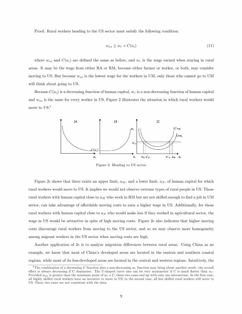
Proof. Rural workers heading to the US sector must satisfy the following condition:

wus ≥ wr + C(ai) (11)

where wus and C(ai) are defined the same as before, and wr is the wage earned when staying in rural

areas. It may be the wage from either RA or RM, because either farmer or worker, or both, may consider

moving to US. But because wus is the lowest wage for the workers in UM, only those who cannot go to UM

will think about going to US.

Because C(ai) is a decreasing function of human capital, wr is a non-decreasing function of human capital

and wus is the same for every worker in US, Figure 2 illustrates the situation in which rural workers would

move to US.9

Figure 2: Heading to US sector

Figure 2c shows that there exists an upper limit, aM , and a lower limit, aN , of human capital for which

rural workers would move to US. It implies we would not observe extreme types of rural people in US. Those

rural workers with human capital close to aM who work in RM but are not skilled enough to find a job in UM

sector, can take advantage of affordable moving costs to earn a higher wage in US. Additionally, for those

rural workers with human capital close to aN who would make less if they worked in agricultural sector, the

wage in US would be attractive in spite of high moving costs. Figure 2c also indicates that higher moving

costs discourage rural workers from moving to the US sector, and so we may observe more homogeneity

among migrant workers in the US sector when moving costs are high.

Another application of 2c is to analyze migration differences between rural areas. Using China as an

example, we know that most of China’s developed areas are located in the eastern and southern coastal

regions, while most of its less-developed areas are located in the central and western regions. Intuitively, the

9The combination of a decreasing C function plus a non-decreasing wr function may bring about another result: the overalleffect is always decreasing if C dominates. The U-shaped curve also can be very asymmetric if C is much flatter than wr .Provided wus is greater than the minimum point of wr +C, these two cases end up with only one intersection. In the first case,all highly skilled rural workers have an incentive to move to US; in the second case, all less skilled rural workers will move toUS. These two cases are not consistent with the data.

9

moving cost for a rural worker from a county close to developed cities is lower than for someone living far

away from them, assuming all other factors are the same– for example, a rural worker from Anhui province

vs. a rural worker from Qinghai province– therefore, given the same wage earned in urban areas, we would

observe less migration from those rural areas located far away from big cities.

Proposition 3 Two different scenarios may appear in rural areas after rural workers move to urban areas

at equilibrium. Rural workers with human capital greater or equal to aN will move to the US sector. Workers

with human capital less than aN could enter RM or stay in RA. These two scenarios are depicted in Figure

3.

Figure 3: Rural career distribution

The mathematical conditions for these two scenarios are shown in Appendix B and C. The intuition is

as follows: fewer rural workers move to the US sector when moving costs are high. This scenario is shown

in Figure 3a. Figure 2c implies that aN in Figure 3a is greater than aN in Figure 3b as the result of lower

moving costs. This implies that rural workers on the lower boundary of migrating flow to US are able to

make higher wages in RM when moving costs are high. This provides room for rural workers with human

capital slightly less than aN to earn higher wages in RM rather than staying in RA after some rural workers

move to US. The rural workers with human capital higher than aL can enter RM after those with human

capital between (aN , aM ) move to US. The departure of some RM workers increases the physical capital per

capita for the remaining RM workers, which encourages more farmers to enter RM. Therefore we may observe

two groups of human capital within which rural workers are in RM: (aL, aN ) and (aM , aX). The values of

aN , aM and aX identify the moving populations and their occupational choices. In rural areas, people with

human capital between aN and aM move to US, while those with human capital greater than aX go to the

UM sector. Because people only move when they can obtain greater benefits, the rural migrant workers and

those former farmers who move to RM are better off. Because the supply of labor in US increases, it reduces

wages in this sector, making the pre-existing urban poor worse off.

10

More rural workers can afford to move to the US sector when moving costs are low. This scenario is

shown in Figure 3b. The marginal worker staying in rural areas possesses less human capital than when

moving costs are high. Because of the low human capital endowments of those who remain in rural areas,

investment cannot support wages in RM higher than those obtained by farming after those with human

capital (aN , aM ) move to cities. In rural areas, people with skills lower than aN work in the agricultural

sector. People with human capital between aN and aM move to US. Those with human capital between

(aM , aX) stay in RM and those with human capital greater than aX will go to the UM sector. All rural

workers with greater human capital than aN are better off. But because the supply of labor in the US sector

increases more than in the first case, it reduces incomes in this sector.

3 Minimum wage

Workers’moving decisions and the market outcomes with free labor mobility may be different with govern-

ment intervention. To avoid a huge migration flow flushing into cities when the labor mobility constraint is

removed, government can use minimum wage policies to smooth the transition, and to maintain subsistent

living standards for low-income workers. Since it is effective to enforce minimum wage on formal sectors, I

assume that minimum wage is imposed on the UM sector at w. It has significant effects on the labor market.

To begin, we consider the UM workers.

Proposition 4 After labor becomes mobile, the minimum wage induces fewer urban workers to enter UM.

The effects on migration to UM depend on the value of the minimum wage. When w is low, it induces more

migrant workers to move to UM, compared to the condition without a minimum wage. When w is high,

migrant workers are limited from moving to UM and less migrant workers move to UM.

Proof. We begin by considering the effects of w on urban workers. Without any migrant workers, the

UM employment is Num = Lu∫ 1

aupuda. When labor is mobile, total employment in the UM sector includes

urban workers and migrant workers. That is, Num = Lu∫ 1

awpuda + NMW where aw is the least human

capital that an urban worker can have and still stay in UM, and NMW > 0 is the number of migrant workers

in UM. When the minimum wage is enforced, it determines the least human capital with which the urban

worker could stay in UM. We have:

w = MPNum(aw,Ku

Lu∫ 1

awpuda+NMW

) (12)

11

For any given urban human capital level, the RHS of equation (12) is less thanMPNum(aw,Ku/Lu∫ 1

awpuda),

which is the wage of urban UM workers when labor is immobile, since each worker will have less physical

capital to work with. Figure 4 shows the effect of w on urban workers.

Figure 4: The effect of w on urban workers

Because w must be greater than wus, aw is greater than aZ . Figure 4 shows that when w is enforced,

the probability of fewer urban workers staying in UM after labor becomes mobile is higher than in the case

without w. If wus drops quickly after labor becomes mobile, we may observe more urban workers in UM

after the labor mobility constraints are removed.

With regard to the rural workers, there are two scenarios. If the MPN of marginal movers when they

work in UM is greater than w, their decision is based on:

MPNUMaX −MPNRM

aX = C(aX) (13)

whereMPNUMaX is the wage if the worker moves to UM andMPNRM

aX is the wage if the same worker stays in

RM. If we keep the same aX as before, since we expect fewer urban workers in UM than in the case without

w, only MPNUMaX is affected, and will be higher than in the case without minimum wage. Therefore, the

LHS of equation (13) must be reduced if it is to hold, which implies that more rural workers are moving to

UM.

Nevertheless, if MPNUMaX < w, then rural workers whose MPN when working in UM is lower than w

are not accepted by any UM firms, because of the enforcement of the minimum wage. In this case theMPN

of the last worker moving to UM must be at least equal to w. That is:

MPNUMaX = w (14)

12

The higher the minimum wage, the less qualified rural workers need be to move to UM. Because w also

equals the MPN of the last urban workers who can stay in UM, the lowest human capital levels are the

same for both urban and rural workers.

The effects of w on the decision to move to US are not certain without making further assumptions about

the properties of the functions. Generally speaking, it is ambiguous because: on the one hand, w drives more

urban workers to the US sector; and because wus is negatively related to the US labor supply, we expect a

lower value of wus with a higher value of w. On the other hand, since w reduces the income in the US sector,

it provides less incentive for rural workers to migrate, which in turn has positive effects on the value of wus.

It is reasonable to expect that high w induces a smaller migration flow to the US sector, since it lowers wus.

The effects of minimum wages will be examined using simulations.

Because the minimum wage policy limits workers from entering UM, it protects UM workers but hurts

US workers, since the US wage is lower with a higher w. The lower w pushes some previous migrant workers

in US back to rural areas, so that employment in RA increases. This obviously hurts the RA workers. The

effects on the welfare of other workers are ambiguous. In the next section, by using data from China, I

simulate a calibrated model to provide various results for different values of w.

4 Numerical analysis

In this section, I first make assumptions on specific functional forms that are consistent with all the previous

assumptions about pdfs of human capital, production functions, wage functions, etc. I use the 2006 data

from China to calibrate my mode, then use the calibrated model to simulate the effects of the minimum

wage policy on the aggregate level and distribution of China’s output. This is an extension of another

calibration which is done by using data from 1986.10 The cut-offs of labor allocations (aN , aM , aX , aZ) are

the endogenous variables in my model. The values of free parameters are either based on real data (Lu, Lr,

Ku, Kr, αu, αr, βu, βr, A), standardized (cr, zrm, za), or derived from theories which are consistent with

the data (cu, zum, a, γ). The outcomes are consistent with all theoretical assumptions.

4.1 Calibration

I assume human capital in both urban and rural areas follows a triangular distribution on the domain

a ∈ (0, 1). The rural distribution peaks at cr and the urban distribution peaks at cu.11 cr is assumed to be

10Please refer to another working paper of mine, China’s internal migration: a theoretical and quantitative analysis, in whichthe calibration is also done using 1986 data.11The pdf of a triangle distribution is triangle shaped. It is 2(x−A)/((B−A)(C−A)) if A ≤ x ≤ C, and it is 2(B−x)/((B−

A)(B − C)) if C ≤ x ≤ B, where A is the lower limit, B is the upper limit and C is the mode.

13

0.3 and cu is 0.6867 which is calibrated when using 1986 data.12 The distribution of urban human capital

thus has first-order stochastic dominance over which of rural human capital.

The manufacturing sector uses a Cobb-Douglas production function:

yim = zim · ai ·Nαi · kβii (15)

RM is more labor intensive and has less value-added than UM.13 Moreover Jin and Du (1997) suggests

that αr is roughly equal to βr for rural industrial sector.14 Given a CRTS production function, they are

both assumed to be 0.5. Sharma (2007) estimates a Cobb-Douglas production function along with a time

trend to capture the effect of technological progress after the reforms in 1978 using a cointegration and

Error-Correction modeling framework for the 1952-1998 period. He found that the output elasticity for

labor was about 0.37 under the assumption of constant returns to scale for all of China. Since rural industry

accounted for roughly 1/5 of total industry, αu = 2/3 and βu = 1/3.15 zrm and zum are free parameters

in my model. Each worker’s physical labor, N , is normalized to 1 in both sectors. The total investment in

urban and rural areas was 2692.03 and 479.47 billion Yuan, respectively, in 1986 prices, which are used to

approximate capital stock.16

The relative price function is derived in Appendix A:

P =yum + yrmA · ya

(16)

The total outputs of the first and second industries were 2473.7 and 10316.2 billion. Considering the

openness of China’s economy in 2006, the ratio between the value of industrial goods and agricultural goods

was about 1:3.6 in China; I assume A = 3.6.17

The wage in the US sector is assumed to be lnwus = γ ln yum − η lnNus. Using data from 1986 to 2008,

I ran a regression of ln(∆yum)) on ln(∆Nus) and ln(∆wus) and have η = 1.23γ.18 Accordingly, the wage

function is assumed to be:

wus =(yum)γ

(Nus)1.23·γ (17)

12Please refer to another working paper of mine: China’s internal migration: a theoretical and quantitative analysis.13Zen (2002) suggested that China’s rural industry is more labor intensive, has a lower added-value and large bulk.14Please refer to Table 3.3 in Jin and Du (1997).15The urban capital share is 0.63-(0.5·1/5)=0.53 and the urban labor share is 0.37-(0.5·1/5)=0.27. The ratio is roughly 2.16Because there is no data on China’s capital stock across periods, I use investment flow to approximate capital stock. We

need very strong economic assumptions to do this approximation, such as assuming the depreciation rate, δ, is very high closeto 1 as K = I/δ at steady state.17This ratio is trade-adjusted. In 2006 China’s net exports totalled 1421.77 billion Yuan and most of it (97.5%) was produced

by the industrial sector. (China Statistical Yearbook, 2007). Those numbers should be subtracted from total outputs to evaluatedomestic preferences.18The coeffi cients of ln(∆Nus) and ln(∆wus) are 1.23 and 0.71 with P-values 1.49E-08 and 8.90E-06. Adjusted R2 is 0.9494.

14

The production function of RA is:

ya = za ·NaA (18)

where a is 0.6091.19 From 1986 to 2006, agricultural output increased by 120%, while agricultural

employment changed from 312.53 million to 325.61 million. By keeping a constant and normalizing za =1

in 1986, za is approximated to be 2.0678 for 2006.

Because workers are free to move between labor markets, all variables are pooled into one equation

system. The moving cost function is assumed to be:

C(a) = cF +1

cV · a2(19)

where cF is the fixed moving cost.20

In 2006, the urban labor force was 283.10 million and the rural labor force was 480.90 million. Of the

131.81 million rural migrant workers, 56.7% went to the industrial sector and 40.5% went to the service

sector.

Based on the information above, the parameters in my current calibration are Lu=283, Lr=481,Ku=2692,

Kr=479, A=3.6, za=2.0678, cr=0.3, cu=0.6867, αr=1/2, βr=1/2, αu=2/3, βu=1/3 and a=0.6091. I have

zrm, zum, cF and cV as the free parameters.

The facts which I have tried to replicate are as follows:

1. In 2006, China’s rural labor force was 480.90 million, and employment in the rural industrial and

private sectors was 194.59 million. I approximate the number of farmers by taking the difference between

these two numbers, which is about 59.53% of the rural labor force.

2. China’s employment in the third industry is 32.20% of the total labor force.

3. After cancelling the manual migration costs imposed by the government, the transportation cost

becomes the major explicit moving cost. In China, long distance travel is mostly by rail. In 2006, the

average rail fare was 57.93 RMB, and, generally, rural workers have to make at least one transfer to reach

the big cities. Therefore, the round-trip fare would be 231.71 RMB, which is 6.45% of a farmer’s income in

2006.

4. Because industrial goods are normalized in my model, the outputs are comparable. The industrial

output in 2006 was 9.33 times that of 1986.

19The value of a is calibrated using the 1986 data. Please refer to another working paper of mine: China’s internal migration:a theoretical and quantitative analysis.20The moving cost function has two parts. The second term is used to approximate non-money costs, though "it would be

diffi cult to quantify these costs" (Sjaastad (1962)).

15

After calibrating, the values of the free parameters are derived as: zrm=0.2181, zum=0.42416, cF=0.0195

and cV=30.219.

4.2 The second best outcome

The second best outcome occurs when utility is maximized aggregately with only one constraint: predeter-

mined capital profile. Because the outputs of different sectors are involved in my model and they are not

comparable, we must resort to the utility function to find the optimal outcome with which the total utility

is maximized. The utility function is assumed to be a Cobb-Douglas, as shown in Appendix A. Calibrated

using the 2006 data, it is

U(xA, xM ) = xA · x3.6M (20)

where xA is the consumption of agricultural goods and xM is the consumption of industrial goods. I

assume consumers have homogeneous preferences, thus every consumer spend the same proportions of her

income on both goods. In the second best case, the marginal product of labor from UM and from RM must

be equalized for the same workers. If aE is the optimal solution to the second best, the workers in both

regions with human capital higher than aE work in either RM or UM sector, and those with lower human

capital work in agricultural sector, based on the assumption that US doesn’t produce real outputs. Therefore

the optimization problem is to maximize equation 20 subject to

αr · zrm · kβrr = αu · zum · kβuu (21)

which comes from MPNrm = MPNum for the same worker. Physical labor is normalized to 1. Since

ki = Ki/Ni where i = rm or um, and Ni is the labor employed in each sector, equation 21 determines

the migration flow: high-skilled rural workers move to the UM sector while low-skilled urban workers move

to the agriculture sector. Because βr and βu are different, the problem is to maximize utility subject to a

non-linear constraint. Given aE , the optimal allocation of labor can be found by equalizing MPNs; then kr

and ku can be expressed as functions of aE , as are the outputs, yum, yrm and ya, since they can be solved

as functions of kr, ku and aE , and since kr and ku are functions of aE . yum, yrm and ya are functions of

aE . Therefore the utility function is also a function of aE and we are able to find the optimal solution to

maximize it.

Instead of solving this complicated non-linear optimization problem, I resort to simulations to find the

optimal solution to it. The second best occurs when the boundary of human capital between the modern

manufacturing sectors and the agricultural sector is 0.6112: those with human capital higher than 0.6112

16

enter either RM or UM, while those with lower human capital enter the agricultural sector. The total

employment in the manufacturing sector is 232.92. But the distribution is very uneven: RM employs only

10.27, while UM employs 222.65, ensuring that a worker makes the same MPN in both sectors. The migration

flow from RM to UM is 93.56.

4.3 The market equilibrium outcome

Due to the friction caused by the existence of moving costs as well as the predetermined capital investment

profile, the optimal market outcome may not be the best. For the same reason, even though minimum wage

is always binding for urban workers, it may or may not be binding for the migrant workers, since they require

higher incomes (and thus have higher MPN) to compensate their moving costs.

The optimal market equilibrium outcome can be solved by maximizing agents’utilities (equation 20)

under certain constraints. To calculate the values of outputs, we need to find the critical values of human

capital had by the marginal workers. The systems of equations which determine the outcomes are different

depending on whether the minimum wage is binding for migrant workers. If it is not binding for migrant

workers, i.e. w < MPNUMaX , the system contains equations 22, 23, 24 and 25.

wus = p · wa + C(aN ) (22)

wus = MPNRMaM + C(aM ) (23)

w = MPNUMaZ (24)

MPNUMaX = MPNRM

aX + C(aX) (25)

Equation 22 implies that the rural workers with human capital aN are indifferent between working in

the RA sector and the US sector. Equation 23 implies that the rural workers with human capital aM are

indifferent between working in RM sector and US sector. Equation 24 implies that the urban workers with

human capital aZ are indifferent between working in the UM sector and the US sector. Equation 25 implies

that the rural workers with human capital aX are indifferent between working in the UM sector and the RM

sector, while migrant workers in the UM sector receive higher wages than the minimum wage. Minimum

wage is binding for urban UM workers only, and all migrants workers in UM earn higher wages than it.

If minimum wage is binding for migrant workers, i.e. w = MPNUMaX , the system is almost the same as

before, only with Equation 25 replaced by Equation 26. Thus it contains equations 22, 23 24 and 26.

17

w = MPNUMaX (26)

Equation 26 defines the human capital, aX , with which rural workers are indifferent between working

in RM and UM when minimum wage is binding for migrant workers as well as for urban UM workers.

Therefore, the optimization problem is to maximize the utility function as given in Equation 20, subject to

the two different equation systems, when w < MPNUMaX or w = MPNUM

aX . Another hidden assumption is

that w must be greater than the market clearing wage.

4.3.1 Simulation

Given the function forms and the calibrated values of parameters, I am able to solve for the optimal value of

the minimum wage and use simulation to visualize its effects on the levels of utilities and outputs, provided

it would yield a better outcome than the market-clearing wage MPNUMaZ . It turns out that the optimal

minimum wage is 0.4814, when minimum wage is just about to be binding for migrant workers. The optimal

utility level is 740.58, compared with the market-clearing UM wage of 0.4725 which yields the utility level

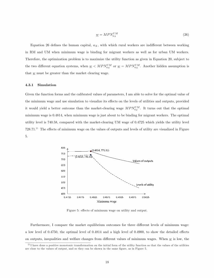
728.71.21 The effects of minimum wage on the values of outputs and levels of utility are visualized in Figure

5.

Figure 5: effects of minimum wage on utility and output.

Furthermore, I compare the market equilibrium outcomes for three different levels of minimum wage:

a low level of 0.4750, the optimal level of 0.4814 and a high level of 0.4900, to show the detailed effects

on outputs, inequalities and welfare changes from different values of minimum wages. When w is low, the

21 I have done a positive monotonic transformation on the initial form of the utility function so that the values of the utilitiesare close to the values of output, and so they can be shown in the same figure, as in Figure 5.

18

minimum wage is not binding for rural migrant workers, though it is just binding when w is optimal, and it

is strictly binding when w is high. The equilibrium outcomes are shown in Table 1.

w aZ aN aM aX ya ym yus

No w 0.6214 0.4678 0.6039 0.6342 64.86 510.74 116.25

Low 0.6237 0.4681 0.6028 0.6329 64.90 511.33 116.35

Optimal 0.6295 0.4690 0.5998 0.6295 64.98 512.78 116.61

High 0.6332 0.4772 0.5971 0.6332 65.80 474.32 105.94

w wus p MPNRA wa MPNaNRM MPNaM

RM MPNaXRM

No w 0.4725 2.1873 0.1380 0.3018 0.2806 0.3623 0.3805

Low 0.4724 2.1887 0.1379 0.3019 0.2810 0.3619 0.3799

Optimal 0.4720 2.1919 0.1378 0.3020 0.2820 0.3606 0.3785

High 0.4386 2.0024 0.1367 0.2738 0.2607 0.3263 0.3460

w MPNaXUM MPNaZ

UM NRA NRM NUM MUM MUS

No w 0.4822 0.4725 286.34 15.83 215.82 91.97 86.87

Low 0.4820 0.4750 286.58 15.81 215.32 92.60 86.01

Optimal 0.4814 0.4814 287.22 15.76 213.99 94.31 83.71

High 0.49 0.49 293.15 19.08 210.23 92.46 76.32

Table 1: Equilibrium outcomes when w is enforced

As w increases, the size of the UM employment becomes smaller, and it decreases by 0.23%, 0.85% and

2.59%, when compared to the case without w. In the US sector, wage decreases by 0.03%, 70.12% and 7.18%.

The income of farmers changes by 0.03%, 0.09% and -9.29%. Regarding migration flows to UM, MUM ,when

w is low, the migration flow is 92.60. It increases to 94.31 when w is the optimal, and decreases to 92.46

when w is high. When w is low, the migration flow to US, MUS , is 86.01. When w is optimal or high, MUS

is 83.71 and 76.32 respectively.

Imposing a minimum wage has significant effects on the values of outputs. Table 2 summarizes the

changes with different minimum wages.

Output value ya ym yus Total value %A

No w 141.88 510.74 116.25 768.87

Low w 142.03 511.44 116.35 769.72 0.11%

Optimal w 142.44 512.78 116.61 771.82 0.38%

High w 131.75 474.32 105.94 712.02 ­7.39%

Table 2: Effects of w on output values

19

An interesting result is seen when the minimum wage is a little higher than the market-clearing wage,

as it helps economic growth. Because of the existence of moving costs, the marginal migrant workers in

UM require higher income when they work in UM than when they work in RM, given there is no minimum

wage. Since only the relatively low-skilled workers in the RM sector would consider moving to US to earn

wus, which is the same as the lowest wage for urban UM workers, the marginal migrant workers (who are

relatively high-skilled) in UM must earn a higher wage than the lowest wage earned by urban UM workers.

This difference provides room for the minimum wage to be set between these two wages. At the time that w

greater than the lowest wage earned by urban UM workers is enforced on urban formal sector, if it is lower

than the wage earned by marginal the migrant workers when there is no minimum wage, it is only binding

for urban workers but not for migrant workers. Thus it drives some urban, low-ability workers at the margin

out of the UM sector, and they are replaced by comparatively high-ability, rural migrant workers. Thus the

output of the UM sector increases. More output from the UM sector, in turn, benefits the workers in the US

and RA sectors. When the minimum wage is high enough to restrain the more effi cient rural workers from

moving, however, it hurts economic growth. We would expect that the higher the minimum wage, the lower

the value of the total output.

With regards to the changes of inequality, I compare the income of workers with human capital equal

to 0.8 with that of the majority in rural areas. Because the gap between capital income and labor income

is the main source of inequality in urban areas, I mean to show the changes of the ratio between capital

income and that of US workers. They illustrate the intra-area inequality change. I also calculate the Gini

coeffi cients, derived from labor income only, since I lack data about the number of capital owners and the

distribution of capital incomes. The inequality changes are shown in Table 3.22

Rural inequality change Urban inequality change Gini

Income ar=0. 8 farmer ratio capital owner US worker ratio

No w 0.6083 0.3018 2.0158 332.66 0.4725 q 0.1470

Low w 0.6093 0.3019 2.0183 333.07 0.4724 1.0015q 0.1473

Optimal w 0.6118 0.3921 2.0254 334.09 0.4720 1.0054q 0.1483

High w 0.6191 0.2738 2.2614 307.67 0.4386 0.9964q 0.1737

Table 3: Effects of w on inequality

In rural areas the workers with human capital of 0.8 work in UM sector. When w is low, their incomes

are 0.6093, which is 2.02 times that of a farmer’s income. When w is set at optimal, in rural areas those

with human capital of 0.8 earn 0.6118, which is 2.03 times that of a farmer’s income. When w is high, in22Because I lack data about the number of capital owners, I assume the ratio between the incomes of capital owners and US

workers is q when no minimum wage is present, given that the income is equally distributed among capital owners.

20

rural areas those with human capital of 0.8 earn 0.6191, which is 2.26 times that of a farmer’s income. Table

6 indicates that inequality becomes worse in rural areas when w increases.

In urban areas the effect of wus is very small when w is low or optimal, and it decreases by 2.35% when

w is high. The income of capital owners changes by 0.36%, 0.43% and -7.51% respectively. The minimum

wage increases the income ratio between capital owners and US workers when it is not binding for migrant

workers, while it decreases this ratio when it is binding for migrant workers. The Gini coeffi cient, which is

based on labor income only, keeps increasing from 0.1470 to 0.1737, suggesting that labor-income inequality

is worsened with higher minimum wage for the whole country.

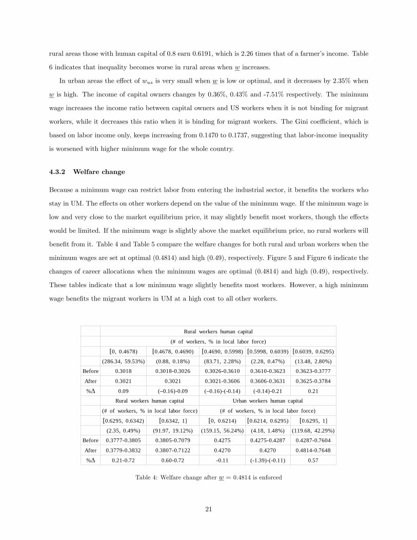
4.3.2 Welfare change

Because a minimum wage can restrict labor from entering the industrial sector, it benefits the workers who

stay in UM. The effects on other workers depend on the value of the minimum wage. If the minimum wage is

low and very close to the market equilibrium price, it may slightly benefit most workers, though the effects

would be limited. If the minimum wage is slightly above the market equilibrium price, no rural workers will

benefit from it. Table 4 and Table 5 compare the welfare changes for both rural and urban workers when the

minimum wages are set at optimal (0.4814) and high (0.49), respectively. Figure 5 and Figure 6 indicate the

changes of career allocations when the minimum wages are optimal (0.4814) and high (0.49), respectively.

These tables indicate that a low minimum wage slightly benefits most workers. However, a high minimum

wage benefits the migrant workers in UM at a high cost to all other workers.

Rural workers human capital

(# of workers, % in local labor force)

[0, 0.4678) [0.4678, 0.4690) [0.4690, 0.5998) [0.5998, 0.6039) [0.6039, 0.6295)

(286.34, 59.53%) (0.88, 0.18%) (83.71, 2.28%) (2.28, 0.47%) (13.48, 2.80%)

Before 0.3018 0.3018­0.3026 0.3026­0.3610 0.3610­0.3623 0.3623­0.3777

After 0.3021 0.3021 0.3021­0.3606 0.3606­0.3631 0.3625­0.3784

%A 0.09 (–0.16)­0.09 (–0.16)­(­0.14) (­0.14)­0.21 0.21

Rural workers human capital Urban workers human capital

(# of workers, % in local labor force) (# of workers, % in local labor force)

[0.6295, 0.6342) [0.6342, 1] [0, 0.6214) [0.6214, 0.6295) [0.6295, 1]

(2.35, 0.49%) (91.97, 19.12%) (159.15, 56.24%) (4.18, 1.48%) (119.68, 42.29%)

Before 0.3777­0.3805 0.3805­0.7079 0.4275 0.4275­0.4287 0.4287­0.7604

After 0.3779­0.3832 0.3807­0.7122 0.4270 0.4270 0.4814­0.7648

%A 0.21­0.72 0.60­0.72 ­0.11 (­1.39)­(­0.11) 0.57

Table 4: Welfare change after w = 0.4814 is enforced

21

Figure 6: Career distribution change after w = 0.4814 is

enforced

Rural workers human capital

(# of workers, % in local labor force)

[0, 0.4678) [0.4678, 0.4772) [0.4772, 0.5971) [0.5971, 0.6039) [0.6039, 0.6332)

(286.34, 59.53%) (6.82, 1.42%) (76.31, 15.87%) (3.74, 0.78%) (15.34, 3.19%)

Before 0.3018 0.3018­0.3080 0.3080­0.3605 0.3605­0.3623 0.3623­0.3799

After 0.2738 0.2738 0.2738­0.3263 0.3263­0.3300 0.3300­0.3460

%A ­9.29 (­11.13)­(­9.29) (­11.13)­(­9.48) (­9.48)­(­8.91) ­8.91

Rural workers human capital Urban workers human capital

(# of workers, % in local labor force) (# of workers, % in local labor force)

[0.6332, 0.6342) [0.6342, 1] [0, 0.6214) [0.6214, 0.6295) [0.6295, 1]

(0.49, 0.10%) (91.97, 19.12%) (159.15, 56.24%) (4.18, 1.48%) (119.68, 42.29%)

Before 0.3799­0.3805 0.3805­0.7079 0.4275 0.4275­0.4815 0.4815­0.7604

After 0.3460­0.3465 0.3884­0.7214 0.4386 0.4386 0.49­0.7739

%A ­8.91 1.90­2.09 ­7.18 (­8.91)­(­7.18) 1.77

Table 5: Welfare change after w = 0.49 is enforced

Figure 7: Career distribution change after w = 0.49 is

enforced

22

5 Policy implications

China adopted a minimum wage policy in the 1990s when its physical labor mobility constraints were virtually

removed. Table 4 shows the effects of enforcing w. First, it protects the insiders in the UM sector by inducing

fewer workers to join UM; thus ku is greater, and every insider would earn a high wage. Nevertheless, the

benefits enjoyed by the UM insiders come at a cost to the majority of other workers in the economy when

the minimum wage is slightly higher than wus, in particular, US and RA workers receive lower incomes. The

effects on RM workers are uncertain: a low w benefits them as more high-ability rural workers leave RM for

UM, while the median and high values of w may hurt them because many high-ability rural workers may

have to stay in RM. Second, enforcing w would have significant effects on migration flows, depending on the

value of w. When w is low, the MPN of the marginal migrant worker to UM is higher. Since fewer urban

workers would stay in UM, the low w would attract more migrant workers to work in UM. The migration

flow to UM would thus be greater than before. In contrast, when w is high, the market equilibrium MPN

of the marginal migrant worker in UM is smaller, and the enforcement of a minimum wage would restrain

rural workers from moving to UM, causing the migration flow to UM to drop. The effect on the migration

flow to US, MUS , depends on two factors: wus and the payoff from the rural sectors. When w increases,

fewer rural workers would be willing to move to US.

An important consideration is the effect of w on the development of the economy as a whole, as well as

on adjustments to social inequality. When the minimum wage is not high enough to constrain the qualified

rural workers from moving to the UM sector, the economic grows, since the low-skilled urban workers are

replaced by relatively high-skilled migrant workers.; on the other hand, a insuffi ciently high minimum wage

hurts economic growth since skilled workers are constrained from entering UM which would reduce aggregate

outputs. In rural areas, a minimum wage enhances inequality: the higher the minimum wage, the worse

the inequality in rural areas. In urban areas, imposing a minimum wage has the opposite effect, inducing a

quicker drop in the capital owners’incomes relative to the incomes of US workers. Thus a high minimum

wage enhances inequality in rural areas, but improves it in urban areas. The combination of imposing a

minimum wage and controlling moving costs may yield a better balance between economic development and

reducing inequality.

Keeping the assumption of surplus labor in the agriculture sector, and focusing on manufacturing sectors

only, when compared with the second best outcome in which the workers with human capital higher than

0.6112 work in the manufacturing sectors, we notice that the RM sector has some lower skilled workers while

the UM sector has higher skilled workers at the market equilibrium. To achieve the second best outcome,

the minimum requirements on human capital must be the same for the RM and UM sectors, implying that

23

aM equals aZ . Since rural workers with aM are indifferent between entering either the US or the RM sectors,

and since urban workers with aZ are indifferent between entering the US or UM sectors, aM is smaller than

aZ provided moving costs exist. Thus, to make them equal, the moving costs must be fully compensated

for those migrant workers moving from RM to US. Such compensation could be provided to encourage the

RM workers at the margin to move to urban areas. Furthermore, since minimum wage policy can be used

to adjust the minimum human capital with which workers stay in the manufacturing sectors, it need not be

binding for migrant workers in UM. Otherwise, since aX equals aZ , aM must be smaller than aZ .

Although China has increased the level of its minimum wages several times recently, many export-oriented

enterprises in eastern coastal areas (even in the central region of China) cannot recruit enough rural migrants

to fill their orders.23 This fact does not imply that my model fails but model parameters or functional forms

change, especially the moving costs (in which the portion of non-money psychic cost has been increasing

dramatically, due to extreme long working hours, wage arrears, etc.). In the meantime, rural workers have

less incentive to move because of the improved working conditions in rural areas. Those changes bring

about transitions back and forth off equilibrium. Even though increasing wages and/or decreasing moving

costs may attract more migrant workers, the enforcement costs would also increase dramatically. Instead,

allocating physical capital by considering the labor force allocation may be more effective in increasing the

output of the manufacturing sectors. This would require a change in government strategy. When urban

areas have significant advantages over rural areas, labor follows capital. Nowadays, since transportation,

medical and education systems have been much improved in rural areas, capital may start to follow labor.

6 Conclusion

In this paper, I present a theoretical model with heterogeneous agents, endogenous internal migration, and

endogenous labor markets, and calibrate this model to analyze the effects of China’s minimum wage policy on

its economic development and inequality issues within the country’s urban and rural areas. Because China’s

government adopted an urban-biased investment strategy since it was founded, the investment decisions

are exogenous in the model as the source of inequality between urban and rural areas. Nevertheless, as

heterogeneous workers are looking for jobs in two regions (urban and rural areas) and across four sectors

(urban modern industry sector (UM), urban subsistence sector (US), rural modern industry sector (RM),

and rural traditional agricultural sector (RA)), at equilibrium, high-ability rural workers go to the UM

sector, while workers who stay in the RM sector may come from two discontinuous groups. All workers

23Please refer to a report, The Investigation on the Shortage of Migrant Workers, which was published by South Weekend(Nanfang Zhoumo) on March 3rd, 2011.

24

who are between the two groups have an incentive to move to the US sector. An enforced minimum wage

may have different effects on the economy, depending on whether or not it is binding for migrant workers in

the urban industrial sector. If not, the minimum wage policy replaces low-skilled urban UM workers with

relatively high-skilled migrant workers, benefiting the whole economy. Otherwise it negatively affects the

whole economy, while helping to slow down the inequality enhancement in cities. To achieve the second best

outcome, full compensation of moving costs should be given to the marginal migrant workers from the RM

to the US sector, and the minimum wage should not be binding for migrant workers in the UM sector.

Although most stylized facts related to China’s internal migration can be explained from my model, it

has several weaknesses that point to possible extensions in future research, besides potential improvement

in specific function forms. First, the economy in my model is assumed to fully follow market principles. In

the real world, however, China is still transitioning from a planned economy to a market economy, though it

has already changed from a closed economy to a large open economy during the process of marketization.24

My model does not capture the price distortion occurring at the beginning of China’s economic reform or

some features of an open economy.25 Second, my model is a static model and no dynamics are included

in the agent’s utility function, while in reality people think not only about their current benefits but also

about their future welfare. This static model also fails to explain the urban-rural inequality change. Third,

though I mention that human capital can be influenced by education and job training, I do not assume

options for agents to accumulate human capital. Because urban areas have better education resources,

another incentive is present for the rural workers to move. Such issues are explicitly clear in Lucas (2004).

Fourth, since no unemployment is present, no uncertainty exists in my model, which is not consistent with

the actual economy. Many economists have presented reasons for unemployment. For example, Harris and

Todaro (1970) proposed a random job selection process over an excess labor supply; Cooper (1985) studied

involuntary unemployment from asymmetric information; and Andolfatto (2008) analyzed unemployment by

using a search model. These authors all provide good hints on how to incorporate unemployment into the

present model.

24China began its economic reform in 1979 and declared its market economy in 1992. As of February 2008, China’s marketeconomy status has not yet been recognized by the US or the EU, though it has been recognized by 77 other countries.25The price scissors between industrial goods and agricultural goods existed in China until 1992 when the country declared

itself as a market economy. See Lin and Yu(2009).

25

Appendix A: relative price forming

Assume the homogeneous utility function over agricultural and industrial goods is:

U(xA, xM ) = xaAxbM (A1)

With different income levels mi and a normalized price of industrial goods, the optimal consumption of

each person is:

x∗A =a

a+ b

mi

P; (A2)

x∗M =b

a+ bmi (A3)

We then have:x∗Ax∗M

=a

b · P (A4)

To clear the market, x∗A/x∗M must equal ya/yM which gives us:

P =a

b(yayM

)−1 (A5)

Generalizing it I assume the relative price forming function as equation (3).

Appendix B: Mathematical equilibrium in Figure 3a

Mathematically, employment levels in the urban sectors, NUS and NUM are defined as:

NUS = Lr

∫ aM

aN

prdar + Lu

∫ aZ

0

pudau (B1)

NUM = Lr

∫ 1

aX

prdar + Lu

∫ 1

aZ

pudau (B2)

Because some previous farmers would move to RM, the employment levels in rural areas now change. Now

a farmer with human capital aL is indifferent between working in RA or RM, and the employment levels in

RA and RM are:

NN = Lr

∫ aL

0

prdar (B3)

26

NRM = Lr

∫ aN

aL

prdar + Lr

∫ aX

aM

prdar (B4)

The relative price, P, is defined as:

P = ρ(ya

yum + yrm) (B5)

where yA, yum and yrm are defined as:

ya = g(NN ) (B6)

yum = Lr

∫ 1

aX

f(ar,Ku

NUM)prdar + Lu

∫ 1

aZ

f(au,Ku

NUM)pudau (B7)

yrm = Lr

∫ aN

aL

f(ar,Kr

NRM)prdar + Lr

∫ aX

aM

f(ar,Kr

NRM)prdar (B8)

At equilibrium, the rural worker with aL must be indifferent between farming and working in RM; that

is:

f ′N (aL,Kr

NRM) = Pg′N (NN ) (B9)

For the rural worker with aN who is indifferent between working in RM and US:

f ′N (aN,Kr

NRM) = wus(yum, NUS)− C(aN ) (B10)

For the rural worker with aM who is indifferent between working in RM and US:

f ′N (aM ,Kr

NRM) = wus(yum, Nus)− C(aM ) (B11)

For the rural worker with aX who is indifferent between working in RM and UM:

f ′N (aX ,Kr

NRM) = f ′N (aX ,

Ku

NUM)− C(aX) (B12)

For the urban worker with aZ who is indifferent between working in US and UM:

wus(yum, Nus) = f ′N (aZ ,Ku

NUM) (B13)

With the expression of P which is shown in equation B5, the equation system with equations B9, B10,

27

B11, B12 and B13 determines the values of aL, aN , aM , aX , aZ . To make extra labor enter RM, at equilibrium

the solutions must satisfy:

f ′N (aN,Kr

NRM) > Pg′(NN ) (B14)

Appendix C: Mathematical equilibrium in Figure 6b

NRM is the employment in RM:

NRM = Lr

∫ aX

aM

prdar (C1)

and the wage of farmers is:

w = Pg′(NN ) (C2)

where P is the relative price which is determined by:

P = ρ(ya

yum + yrm) (C3)

where yA, yum and yrm are the equilibrium outputs of RA, RM and UM sectors, which are defined in

equations C7, C8, and C9.

The employment levels of RA, US and UM are:

NN = Lr

∫ aN

0

prdar (C4)

NUS = Lr

∫ aM

aN

prdar + Lu

∫ aZ

0

pudau (C5)

NUM = Lr

∫ 1

aX

prdar + Lu

∫ 1

aZ

pudau (C6)

The outputs of RA, RM and UM are:

ya = g(NN ) (C7)

yrm = Lr

∫ aX

aM

h(ar,Kr

NRM)prdar (C8)

28

yum = Lr

∫ 1

aX

f(ar,Ku

NUM)prdar + Lu

∫ 1

aZ

f(au,Ku

NUM)pudau (C9)

The rural worker with aN must be indifferent between working in agricultural and US; that is:

Pg′(NN ) = wus(yum, Nus)− C(aN ) (C10)

The rural worker with aM must be indifferent between working in RM and US; that is:

MPNrm(aM ,Kr

NRM) = wus(yum, Nus)− C(aM ) (C11)

The rural worker with aX must be indifferent between working in RM and UM; that is:

MPNrm(aX ,Kr

NRM) = MPNum(aX ,

Ku

NUM)− C(aX) (C12)

The urban worker with aZ must be indifferent between working in US and UM; that is:

wus(yum, Nus) = MPNum(aZ ,Ku

NUM) (C13)

Because my employment functions and output functions are all of aN , aM , aX and aZ , the equilibrium

values are determined by solving the equation system containing C10, C11, C12, and C13. To make no extra

labor enter RM, at equilibrium the solutions must satisfy:

MPNrm(aN ,Kr

NM) < Pg′(NN ) (C14)

29

References

[1] Andofatto, D., 2008. Search Models of Unemployment. The New Palgrave Dictionary of Economics, 2nd

edition.

[2] Ashenfelter, O., Farber, H., Ransom, M., 2010. Labor Market Monopsony. Journal of Labor Economics.

28(2), 203—210.

[3] Au, C., Henderson, J., 2006. How Migration Restrictions Limit Agglomeration and Productivity in

China. Journal of Development Economics. 80(2), 350—388.

[4] Boal, W., Ransom, M., 1997. Monopsony in the Labor Market. Journal of Economic Literature. 35(1),

86—112.

[5] Borjas, G., 1987. Self-Selection and the Earnings of Immigrants. The American Economic Review. 77,

531—553.

[6] Broadway, R., Cuff, K. 2001. A minimum wage can be welfare-improving and employment-enhancing.

European Economic Review. 45, 553—576.

[7] Cheng, Y., 2007. The Evolution of China’s Gini Coeffi cient and Its Decomposition Between Urban

and Rural Areas After Economic Reform (in Chinese: Gaige Yilai Chengxiang Zhongti Gini Xishu de

Yanbian Jiqi Chengxiang Fenjie). China’s Social Science (Zhongguo Shehui Kexue). 4.

[8] Cole, W., Sanders, R., 1985. Internal Migration and Urban Employment in the Third World. The

American Economic Review, 75(3), 481—494.

[9] Cooper, R., 1985. Worker Asymmetric Information and Involuntary Unemployment. Journal of Labor

Economics. 3(2), 188—208.

[10] Drazen, A., 1986. Optimal Minimum Wage Legislation. The Economic Journal. 96, 774—784.

[11] Du, Y., Park, A., Wang, S., 2005. Migration and Rural Poverty in China. Journal of Comparative

Economics. 33, 688—709.

[12] Guo, X., 2004. A New Estimation of the Income Gap Between Rural and Urban Areas (in Chinese:

Chenxiang Shouru Chaju de Xinguji). Shanghai Economic Study (Shanghai Jinji Yanjiu). 12.

[13] Harris, J., Todaro, M., 1970. Migration, Unemployment and Development: A Two-sector Analysis. The

American Economic Review. 60(1), 126—142.

30

[14] Jin, H., Du, Z., 1997. Productivity of China’s Rural Industry in the 1980’s. Chinese Economics Research

Center (CERC) working papers. 1997-06.

[15] Kung, J., Lin, Y., 2007. The Decline of Township-and-village Enterprises in China’s Economic Transi-

tion. World Development. 35(4), 569—584.

[16] Krusekopf, C., 2002. Diversity in Land-tenure Arrangements Under the Household Responsibility System

In China. China Economic Review. 13, 297—312.

[17] Lin, J., Yu, M., 2009. The Political Economic Analysis of China’s Price Scissors: Theory Model and

Empirical Evidence (in Chinese: Wogou Jiage Jiandaocha de Zhengzhi Jingjixue Fenxi: Lilun Moxin

Yu Jiliang Shizheng). Economic Study (Jingji Yanjiu), 1, 422—456.

[18] Lu, Y., 2002. China’s Hukou System After 1949: Structure and Evolution (in Chinese: 1949 Nian Hou

De Zhonggou Huji Zhidu: Jiegou Yu Bianqian). Jounal of Peking University (Beijing Daxue Xuebao).

2.

[19] Lucas, R., 2004. Life Earnings and Rural-Urban Migration. Journal of Political Economy. 112(1), S29—

S59.

[20] Naughton, B., 2007. The Chinese Economy: Transitions and Growth. MIT Press. Cambridge.

[21] Pan, X., Sun, G., 2008. A Survey and Analysis on the Education of the Children of Migrant Workers

(in Chinese: Jincheng Mingong Zinu Jiating Jiaoyu De Diaocha Yu Fenxi). Journal of the Party School

of CPC Hangzhou (Zhonggong Hangzhou Shiwei Dangxiao Xuebao). 4.

[22] Ravallion, M., and Chen, S., 2007. China’s (uneven) progress against poverty. Journal of Development

Economics. 82, 1—42.

[23] Roy, A.D., 1951. Some Thoughts on the Distribution of Earnings. Oxford Economic Papers. 3, 1352—146.

[24] Sharma, H., 2007. Sources of Economic Growth in China, 1952-1998. Issues in Political Economy, 17.

[25] Shoven, J., and Whalley, J. 1992. Applying General Equilibrium. Cambridge University Press.

[26] Sjaastad, L., 1962. The Costs and Returns of Human Migration. The Journal of Political Economy.

70(5), 80—93.

[27] Strobl E., Walsh F., 2007. Dealing with monopsony power: Employment subsidies vs. minimum wages.

Economics Letters. 94, 83—89.

31

[28] Wang, F., Zuo, X., 1999. Inside China’s Cities: Institutional Barriers and Opportunities for Urban

Migrants. The American Economic Review. 89, 276—280.

[29] Watanabe, S. 1976. Minimum wages in developing countries: myth and reality. International Labour

Review. 113, 345—58.

[30] Whalley, J., Zhang, S., 2007. A Numerical Simulation Analysis of (Hukou) Labour Mobility Restrictions

in China. Journal of Development Economics. 83, 392—410.

[31] Yang, D., 1999. Urban-Biased Policies and Rising Income Inequality in China. The American Economic

Review. 89(2), 306—310

[32] Yao, S., 1994. Agricultural Reforms and Grain Production in Rural China. Palgrave Macmillan.

[33] Zen, F., 2002. On the Interaction of Urbanization and Industry Sturcture (in Chinese: Lun Chengshihua

Yu Chanye Jiegou De Hudong Guanxi). Economic Review (Jingji Zhongheng), 10.

[34] Zhang, K., Song, S., 2003. Rural—urban Migration and Urbanization in China: Evidence from time-series

and cross-section analyses. China Economic Review. 14, 386—400.

[35] Zhao, Y., 1999. Labor Migration and Earnings Differences: The Case of Rural China. Economic Devel-

opment and Cultural Change. 47(4), 767—782.

[36] Zhang, W., Lei, K., 2008. The Analysis of the Structure, Status Quo and Determinants of a New

Urban Migrant’s Social Integration (in Chinese: Chengshi Xinyimin Shehui Ronghe). Sociology Study

(Shehuixue Yanjiu). 5.

32