The Economic Consequences of Excess Men:

Evidence from a Natural Experiment in Taiwan

Simon Chang, Assistant professor

Central University of Finance and Economics

Xiaobo Zhang, Senior research fellow

International Food Policy Research Institute

Abstract

Sex ratio imbalances have become a problem in an increasing number of countries. In this paper, we use a natural experiment in Taiwan to test the economic consequences of excess men. With the defeat of the Kuomintang Party in China, more than one million soldiers and civilians, mainly young males, retreated to Taiwan in the late 1940s. Initially, the soldiers from mainland China were not allowed to marry. The ban was relaxed in 1959, however, suddenly flooding the marriage market with a large number of eligible bachelors. The operational ratio of males to females at marriageable age peaked at nearly 1.2 in the 1960s. Using data from multiple sources, we find that during times of high marriage competition, young men are more likely to become entrepreneurs, work longer hours, save more, and amass more assets. The findings highlight the important role of biological forces in shaping human economic behavior.

Keywords: sex ratios; mating competition; entrepreneurship, and Taiwan.

1

1. Introduction

Survival and reproduction are two fundamental motives for all species of life (Darwin 1871). Charles Darwin’s thinking on natural selection (survival of the fittest) was deeply influenced by Thomas Malthus, a leading economist at the time. However, Darwin noted that natural selection does not explain all traits in the biological world. The ornate plumage of male peacocks is a classic example. Even though, to a large extent, the long tails inhibit male peacocks from escaping predators in densely wooded area, the feathers are appealing to female peacocks. Having the trait of extravagantly colorful feathers enhances the male peacocks’ chances for mating and reproductive success. Darwin defined sexual selection as competition within a species for the purpose of reproduction. Sexual selection is widely observed in mammals, wherein members of the less limited sex, typically males, compete aggressively in deterring rivals and attracting mates in order to maximize their reproductive success.

Darwin conjectured that some human biological features, such as beards, can be better explained by sexual selection than by natural selection. Some economists (Cox 2007; Frank 2011) maintained that the insight of Darwinian sexual selection can shed light on the understanding of human economic behavior, especially in situations in which rewards are based on relative positions, such as in polygamous marriage markets, pollution control, and housing regulations. Despite their biological roots, humans differ in many ways from their biological ancestors, including in their use of markets for exchange. Therefore, it is important to take specific human characteristics into account when analyzing the economic implications of Darwinian sexual selection. For example, in the marriage market of contemporary industrial society, women rank men’s earning capacity as more important than their appearance (Buss 1989), a trait valued highly among female mammals. If the mechanism of sexual selection holds true for humans, we would expect to see men compete among each other to increase their earnings and enhance their chance of securing mates.

In most human societies, sex ratios (male-to-female ratios) at the marriageable age are roughly balanced.1 Due to a lack of variation in sex ratios, it is extremely challenging to find compelling evidence to directly test sexual selection specific to humans. Unlike in the natural sciences, it is unethical to run randomized experiments to test this theory by manipulating sex ratios and measuring their impact. This is perhaps one reason that the empirical literature on the impact of sexual selections on human economic behavior is still sparse. Despite the challenge, however, some researchers have tried to tackle the question using various approaches. 1 In the human biology literature, the sex ratio at the mating age is often called operational sex ratio.

2

The first approach is to manipulate skewed sex ratios in a lab setting. For example, Griskevicius et al. (2012) presented different groups of lab participants with either more male or more female images. They found that men who are shown a higher proportion of male images are more likely to engage in conspicuous consumption and pursue intermediate financial gains, whereas female participants were not sensitive to the manipulated sex ratios at all. However, it is not clear whether the economic effects of the manipulated sex ratios demonstrated in the lab settings are instantaneous or lasting. Nor is it clear what the ramifications are in the real world, where sex ratio imbalances normally persist for a much longer time.

The second method is to use survey data, as represented by Nettle and Pollet (2008). Based on survey data form the National Child Development Study in the United Kingdom, the authors reported that richer men are much less likely to be childless than their poor counterparts. In lieu of this evidence, the authors concluded that wealth helps increase men’s likelihood of reproductive success. However, due to the nature of the data, it is hard to rule out the reverse causality—that is, men with a greater number of children may be forced to work harder and accumulate more wealth. Moreover, the male-to-female ratios in Britain are largely balanced, making it difficult to disentangle the associations among mating competition, wealth creation, and reproductive success.

The third method is to take advantage of spatial variations in sex ratios observed in the real world. For example, Angrist (2002) found that in US cities with a larger sex ratio imbalance (more men than women), women have a greater likelihood of getting married and opting out of the labor market. Because labor is fully mobile in the United States, the observed spatial difference in sex ratios is likely endogenous—that is, some unobserved factors may determine both the economic outcomes and the number of men and women in the workforce in a particular location. To address the potential endogeneity problem, the author used the flow of immigrants in previous generations to instrument the sex ratio variable. However, he did not elaborate on the effect of mating competition on men’s economic behavior, which is a focus of our paper.

Following the same spirit, by making use of the large regional and temporal variations in sex ratios in China that resulted from a combination of implementing the one-child policy, the spread of ultrasound technology, and the cultural preference for sons over daughters, Wei and Zhang (2011a, 2011b) showed that parents with sons increase their savings and are more actively engaged in entrepreneurial activities in regions with more skewed sex ratios. The authors used regional variations in the implementation of the one-child policy as an instrument for the sex ratio variable. However, because the one-child generation was still too young to participate in economic activities in the years the

3

population censuses and surveys used in the studies were conducted, the authors instead focused on parental responses to mating competition in their children’s cohort.

It should be noted that the findings in Wei and Zhang (2011a) on savings contradict those reported in Griskevicius et al. (2012), who found that high sex ratios reduce young men’s savings. The contradiction may be explained by two factors. First, parents and children may respond to the marriage market squeeze differently. Second, people may behave differently when facing an artificial sex ratio imbalance in labs versus an actual imbalance in the real world. Therefore, the best way to reconcile the results is to use a natural experiment in the real world, where the variation in sex ratios is caused by exogenous factors, independent of economic outcomes.

In this paper, we directly examine the economic effects of a tightening marriage market on young men by using a powerful natural experiment in Taiwan. After their defeat by the Chinese Communist Party, more than one million Chinese Nationalist Party (also known as Kuomintang) soldiers and civilians, mostly young and unmarried, fled to Taiwan in the late 1940s. Such a massive influx of young males from mainland China created a human-made marriage market squeeze in Taiwan, which had a population of only about six million people at the time. The sex ratio among the 20–24 age cohort reached as high as 152 men for every 200 women in 1950 (Francis 2011). Chiang Kai-shek wanted his solders to be ready at any time for counterattacking mainland China, instead of settling in Taiwan. So the Kuomintang government imposed a marriage ban on soldiers in the early 1950s; this ban was not lifted until 1959. The flood of immigrants and the subsequent marriage regulations offer a natural laboratory in which to examine the economic implications of having too many men.

Based on the timing of imposing and removing marriage bans on soldiers in service, we impute operational sex ratios for the marriage-age cohort at the county level over time and directly test the economic consequences of excess men. Using data from multiple sources, we show that an excess supply of men in the marriage market stimulates men’s animal spirit to participate in more entrepreneurial activities, work longer hours, and amass more assets.2

2 Our study is different from Francis (2011), who computed operational sex ratios at the regional level in Taiwan and investigated the impact of skewed sex ratios on women and children based on the intrahousehold bargaining literature. He found that increasing the sex ratio imbalance augments women’s bargaining power in several dimensions, including fewer children in a family and greater human capital investment in children. In this paper, we impute sex ratios at the more disaggregate county level and improve his computations by taking into account the timing of imposing and removing the marriage bans on soldiers in service. Another key departure from his study is that we primarily investigate the economic consequences of sex ratio imbalance on men, especially on their entrepreneurship.

4

Apart from testing the effect of mating competition on men’s economic behavior, this paper also provides a new lens through which to examine Taiwan’s economic miracle. Taiwan transformed itself from an agrarian economy to a newly industrialized society in just several decades. There is no doubt that many factors contributed to Taiwan’s economic miracle.3 However, the demographic shock induced by massive male-dominated immigrants has never been mentioned in the literature as a contributing factor in Taiwan’s rapid economic growth. We show in this paper that over the past six decades, growth in the number of newly registered private enterprises, the gross domestic product (GDP), and exports closely matched temporal patterns of the operational sex ratio. In short, Taiwan’s economic miracle may have something to do with sexual selection in the marriage market.

This paper is arranged as follows. The next section provides a brief literature review. Section 3 describes the historical background and the imputation procedures of operational sex ratios and relates them to Taiwan’s general economic patterns. Section 4 shows the discovery that being an entrepreneur is associated with reproductive success—that is, a greater likelihood of marriage and a lower probability of being childless. This finding establishes the fact that women do regard entrepreneurship as a desirable trait in the marriage market. In Section 5, using data from multiple sources, we unravel evidence that shows that in regions with more skewed operational sex ratios, men are more likely to engage in entrepreneurial activities, work longer hours, save more, and accumulate more wealth. Section 6 concludes.

3 There are numerous explanations for Taiwan’s economic miracle, including land reform, accumulation of human capital, demographic change, and active industrial policy (Lucas 1993; Stiglitz 1996; Bloom and Williamson 1998).

5

2. Literature Review

The idea that mating competition intensifies men’s pursuit for wealth can be traced through several strands of literature. In the evolutionary biology literature, Trivers and Willard (1973) theorized that as long as there is sexual dimorphism (a phenotypic difference between males and females) in the investment costs of raising offspring, males and females will adopt different mating strategies. In humans, women spend more time taking care of newborns and have a shorter reproductive clock than their male counterparts; thus, women are the limiting factor in human reproduction. As a result, men tend to compete for women, whereas women choose mates who can provide more resources to support their offspring. Thus, if women regard wealth as a desirable trait in men, then men would strive to accumulate wealth to enhance their attractiveness.

The theoretical economics literature on status demonstrates that the concerns for status (that is, relative position in a society) matter to human economic behavior.4 Cole, Mailath, and Postlewaite (1992) showed that income can become a key sorting variable in the marriage market, inducing men to work harder to increase their earnings. Consequently, mating competition could stimulate economic growth. Note that the authors assumed a balanced male-to-female ratio. If the ratio were skewed in favor of women, it is expected that men would compete even harder, thereby making a greater contribution to economic growth.

Hopkins and Kornienko (2010) developed a theoretical model showing that when society allocates resources according to relative positions and when stakes (both rewards and risks) are high, those at the bottom of the status gradient expend greater effort than do their rich counterparts.5 Although the model does not explicitly distinguish between men and women, it sheds some light on the consequence of mating competitions on men’s behavior in the wake of female shortages. Suppose the model referred to men and that the rewards were mating partners. When women are in short supply, a certain number of men are doomed to stay single. Facing such a dire consequence, those men at the lower economic order are forced to work harder in an attempt to outpace others. In a sense, the model implicitly predicts that an increase in the ratio of men to women forces men to exert greater effort.

Robson (1992) developed a theoretical model to explain the relationship among the concerns for status, distribution of wealth, and risk attitude. He found that if the gain in 4 A large thread of the status literature focuses on conspicuous consumption and other negative externalities (Frank 1985, 2004, 2007). 5 The rewards can be negative for losers.

6

status owing to wealth increase outstripped the loss in status associated with the same amount of wealth reduction, taking gambles would be a better strategy than maintaining status quo. According to the model, if there were excess men in the marriage market, men lower in the pecking order would take more economic risks, because a win would greatly lift their status and increase their chance of finding a mate. Conversely, if the gamble fails, their position at the nadir and their existing grim chance for marriage would hardly be affected.

Since different occupations imply different earning potentials, the preference for wealth in the marriage market can shape people’s job choices. For example, entrepreneurs, on average, earn more than regular salaried workers while also bearing larger risks. When facing a shortage of women, all of the aforementioned theoretical models predict that men are more likely to engage in entrepreneurial activities in the hopes of amassing more wealth to increase their odds of marriage. We aim to empirically test this hypothesis in this paper.

Du and Wei (2011) developed an overlapping generation model with one representative man and one representative woman to explicitly examine the impact of sex ratio imbalance on men’s entrepreneurial activities. Their model assumes that both men and women have the identical utility function, including wealth and emotional components, except that only men can choose to be entrepreneurs. Men and women are matched based on their utility level. By choosing to be an entrepreneur, a man increases his chance of getting married if his business succeeds. However, in the event of failure, he may end up with no wife at all. The model predicts that as the ratio of males to females rises—as long as the ratio remains below a threshold—a greater number of men will choose to become entrepreneurs.

Compared with the large body of theoretical literature, the empirical literature on the economic consequences of sexual selection is scant. Angrist (2002) was one of the earliest empirical papers on this topic, focusing on the impact of sex ratio on women’s labor market outcomes. Although the paper briefly mentions that higher sex ratios augment men’s earnings, it does not explicitly link the results with Darwinian sexual selection, which is central to our paper.

Wei and Zhang (2011b) presented evidence that parents with sons respond to the unfavorable marriage market in their sons’ cohort by working harder, undertaking dangerous or unpleasant jobs, and setting up businesses. In addition, they postpone consumption in favor of wealth accumulation (Wei and Zhang 2011a). In short, parents respond to shifts in their children’s marriage market through their own economic behavior. However, the authors did not discuss the economic effects on the young men

7

themselves. According to Darwinian sexual selection, it is the young men who should compete with each other when facing dire marriage prospects. After all, they are directly exposed to the marriage market squeeze.

In many cultures, bride prices (transfers from a groom family to a bride family) and dowries (transfers from a bride family to a groom family) are prevalent. To a large extent, bride prices and dowries reflect the demand and supply of men and women in the marriage market. In places with more women seeking partners, such as India in the 1980s, the terms of trade favor groom families, allowing them to receive high dowries (Rao 1993; Edlund 2000). Conversely, if there were more men seeking partners, dowry payments would come down and bride prices would go up, as shown by Brown, Bulte, and Zhang (2011) and Francis (2011).

When exposed to an excess supply of men, married women are also more likely to gain bargaining power within a household. Consistent with the theory of Becker (1981), Francis (2011) found that women in Taiwan prefer to have fewer children when facing more favorable terms of trade. Likewise, Porter (2011) showed that in areas with a higher male-to-female sex ratio, women provide more support to their own parents and less to their husbands’ family.

The negative social consequences of sex ratio imbalances have also been reported. Edlund et al. (2007) found that crime rates in China are higher in regions with more skewed sex ratios. Den Boer and Hudson (2004) even warned that countries with excess men are more likely to wage wars.

Our paper also connects to the literature on the causes of sex ratio imbalances. Son preference is often regarded as a contributing factor to skewed sex ratios (Edlund 1999; Das Gupta 2005). In addition, the widespread adoption of affordable ultrasound technology (Li and Zheng 2009), family planning policies (Bulte, Heerink, and Zhang 2011; Ebenstein 2010), and lower earnings for women (Qian 2008) are also listed as potential causes of China’s rising sex ratio imbalance.

8

3. Historical Background and Data

Historical Background

In mainland China, the end of World War II was immediately followed by a civil war between the Chinese Nationalist Party (Kuomintang) and the Chinese Communist Party from 1945 to 1949. The former was defeated and retreated to Taiwan with a great number of followers, including soldiers and civilians. Various studies have suggested that the number of civil war immigrants to Taiwan ranged between 0.6 and 1.25 million, whereas Taiwan’s local population was only 6 million (Barclay 1954; Jacoby 1967; Ho 1978; Chen and Yeh 1982; Liu 1986; Lin 2002). Among the immigrants, the number of soldiers, who were mostly single males in their early 20s, is estimated to be between 0.55 and 0.6 million. It is thus not surprising that the composition of the immigrants was highly male-biased. Francis (2011) suggested that within the immigrants, men outnumbered women by a factor of 4 to 1, which led to a significant sudden rise in Taiwan’s sex ratio.

To prepare for counterattacking mainland China, the soldiers of the Chinese Nationalist Party were not allowed to get married in the 1950s (Lin 2002). In 1952, the marriage ban was formally written into a law called the Military Marriage Ordinance (MMO).6 The MMO forbade most active military personnel from getting married, except for military officers and technician sergeants. However, in August 1959, the ban was relaxed for most soldiers, except for male soldiers younger than 25 years of age, female soldiers younger than 20, and all soldiers who had served fewer than 3 years.7 This relaxation essentially made the MMO nonbinding for most immigrant soldiers, who either were already older than 25 or had served more than 3 years by 1959, which meant that they could finally get married roughly 10 years after they had retreated to Taiwan.

Meanwhile, in the mid-1950s, the Chinese Nationalist Party had begun to conscript young Taiwanese men to replace aging immigrant soldiers. In principle, conscripted Taiwanese men were also subject to the marriage ban. However, unlike their immigrant counterparts, Taiwanese soldiers generally served for a much shorter period and remained socially connected to others outside the military while in the military.8

Imputing Operational Sex Ratios

6 The ban was de facto effective even before the law was enacted. 7 In 1974, the MMO was further relaxed to include only soldiers currently involved in combats and students in military academies. It was completely repealed in 2005. 8 Taiwanese soldiers generally served in their early 20s for 2 or 3 years.

9

In Taiwan, the official population data are collected through a civilian household registration system. However, prior to 1969, active military personnel were generally excluded from the civilian registration system, unless they got married (Lin 2002). In November 1968, this exclusion was changed by an executive order that required all military personnel to be registered in the civilian system. This implies that until 1969, immigrant soldiers tended not to show up in official population data. Consequently, the raw sex ratio that was calculated from official population data before 1969 is biased.

Because of the bias of the raw sex ratio, in this study we impute an operational sex ratio that better reflects the intensity of competition in the marriage market. The immigrant soldiers are excluded in the calculation of operational sex ratios before 1960 because they were effectively subject to the MMO. However, the Taiwanese soldiers are still included in the operational sex ratio, because of their short duration of service and strong social ties, even though they were also subject to the MMO. In this paper, we mainly adopt the imputation method proposed by Chang (2011). The details of the imputation procedure are provided in the appendix.

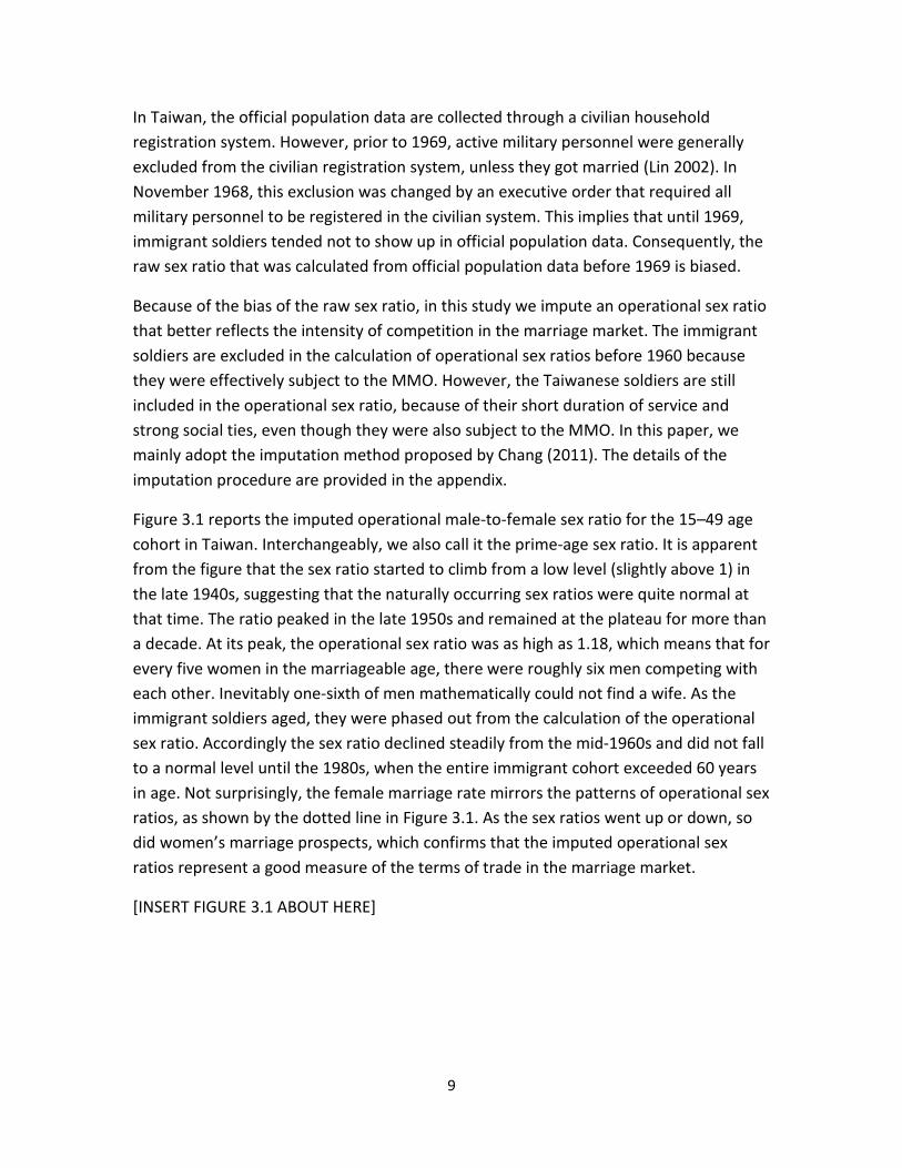
Figure 3.1 reports the imputed operational male-to-female sex ratio for the 15–49 age cohort in Taiwan. Interchangeably, we also call it the prime-age sex ratio. It is apparent from the figure that the sex ratio started to climb from a low level (slightly above 1) in the late 1940s, suggesting that the naturally occurring sex ratios were quite normal at that time. The ratio peaked in the late 1950s and remained at the plateau for more than a decade. At its peak, the operational sex ratio was as high as 1.18, which means that for every five women in the marriageable age, there were roughly six men competing with each other. Inevitably one-sixth of men mathematically could not find a wife. As the immigrant soldiers aged, they were phased out from the calculation of the operational sex ratio. Accordingly the sex ratio declined steadily from the mid-1960s and did not fall to a normal level until the 1980s, when the entire immigrant cohort exceeded 60 years in age. Not surprisingly, the female marriage rate mirrors the patterns of operational sex ratios, as shown by the dotted line in Figure 3.1. As the sex ratios went up or down, so did women’s marriage prospects, which confirms that the imputed operational sex ratios represent a good measure of the terms of trade in the marriage market.

[INSERT FIGURE 3.1 ABOUT HERE]

10

4. Entrepreneurship as a Desirable Trait in the Marriage Market

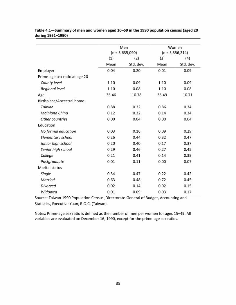
It has been widely documented that wealth is an important status variable in the human marriage market (Buss 1989). When all else is held constant, women prefer to marry rich men. Since entrepreneurs, on average, are wealthier than the general population, it is expected that male entrepreneurs are more successful in attracting mating partners than are ordinary male workers. We use Taiwan Population Census 1990 data to verify this theory. The census includes detailed demographic information for all individuals, including age, sex, education level, and occupations. We extract from the census a sample consisting of all individuals aged 20–59. The oldest cohort was age 20 in 1951 and the youngest reached 20 in 1990.

Table 4.1 lists the sample summary statistics. As revealed in the table, the operational sex ratio for the sample at age 20 averages at 1.10, which is much higher than natural. Using the sample, we regress men’s and women’s marital status on their entrepreneurial status, by controlling for a set of personal characteristics, such as age, education, birthplace, and a full set of county fixed effects. An individual is defined as an employer and assigned a value of 1 if that person owned a business and hired workers. Table 4.2 reports the regression results. The coefficient for the entrepreneurial status variable in the regression on men is 0.145 and is highly significant at a 1 percent level, which means that being an entrepreneur enhances a man’s likelihood of marriage by 15 percent. In contrast, the coefficient is statistically insignificant in the regression on women. In other words, being an entrepreneur improves a man’s mating success but not a woman’s. Education also matters to marriage prospects. Educated men are more likely to get married than their illiterate counterparts. However, for women, those with elementary education have the higher rate of marriage, whereas those with a college degree have a lower likelihood of marriage than those who are less educated.

[INSERT TABLES 4.1 and 4.2 ABOUT HERE]

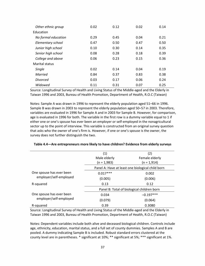
Marriage is a prerequisite for having a child in Chinese culture. If being an entrepreneur boosts a man’s odds of marriage, then naturally it would make him more fecund. The longitudinal Survey of Health and Living Status of the Middle Aged and the Elderly in Taiwan for 1996 and 2003 includes information about the fertility history of each respondent. We can use this dataset to investigate whether entrepreneurship lowers a man’s likelihood of being childless. As reported in Table 4.3, on average, each elderly person in Samples A and B has about four and three biological children, respectively, but 3 percent and 6 percent, respectively, of them are childless. In addition, the survey provides the employment history of the elderly. About 22 percent and 31 percent of the

11

elderly or their spouse in samples A and B, respectively, have ever been a nonagricultural employer or self-employed in their life.9

[INSERT TABLE 4.3 ABOUT HERE]

Table 4.4 reports the regression results using the pooled data of both samples. The outcome variable in Panel A is whether a person has ever had a biological child (including both children who are alive or deceased). Engaging in entrepreneurial activities drops a man’s odds of never having a child by 28 percent (0.017/0.06*100).

[INSERT TABLE 4.4 ABOUT HERE]

In Panel B, we replace the outcome variable in Panel A with total number of children ever born. The coefficient for the entrepreneurship variable remains positive (even larger in magnitude than in Panel A), but it loses significance. The ideal number of children one wants to bear may have a nonlinear relationship with one’s entrepreneurship status. Having at least one surviving child perhaps is a top priority for most people, including entrepreneurs. It is well known that entrepreneurs work strenuous hours. Entrepreneurs may have to reduce working hours and forgo earning potentials, which are normally larger than salaried employees, if they have to raise additional children. The opportunity cost to bear a child is particularly high for female entrepreneurs. The regressions on the total number of biological children reported in Panel B confirm the point that female entrepreneurs produce fewer children relative to ordinary female workers and stay-at-home moms. Entrepreneurship status does not matter much to the total number of children for men. If a man has already had a child, being an entrepreneur does not necessarily result in a higher fertility rate. The results are consistent with the findings reported in Nettle and Pollet (2008) for the United Kingdom.

9 The employer or self-employed information is based on a series of employment questions. For each job that one has ever taken, the survey asks the respondent who the owner of the business is. One option is that the owner is oneself or a spouse. Unfortunately, the survey does not further separate the two cases. We thus define the entrepreneurship variable as 1 if the respondent or the spouse has ever worked as a business owner or has been self-employed in nonagricultural sectors and as 0 if the respondent has never worked or has worked only as an employee. This survey method overestimates the prevalence of entrepreneurship. Despite the caveat, it is the only dataset available that includes detailed fertility history. One should bear this shortcoming in mind when reading the results based on the dataset.

12

5. Statistical Evidence

Descriptive Evidence

In most societies, sex ratios at the marriageable age are largely balanced. Thus it is challenging to measure the degree of mating competition and examine its consequences on entrepreneurship. The large variation in sex ratios in Taiwan allows us to directly gauge the link between varying degrees of mating competition and entrepreneurship across space and time.

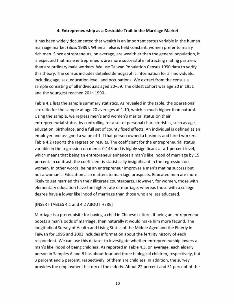
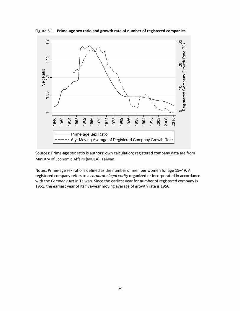
We first plot the time series of sex ratio and extensive growth in the number of firms at the aggregative level (Figure 5.1). As clearly indicated in the figure, the two lines representing the operational sex ratio and the five-year moving average of the extensive firm growth rate move in sync throughout the entire sample period, which spans 55 years. Of course, this figure is just for illustrative purpose, and the tentative evidence does not stand for any causal relationship. To show the causality of sex ratios on entrepreneurship, we conduct a more rigorous quantitative analysis by making use of individual and household-level data, as well as regional and temporal variations in sex ratios.

[INSERT FIGURE 5.1 ABOUT HERE]

Sex Ratios and Entrepreneurship

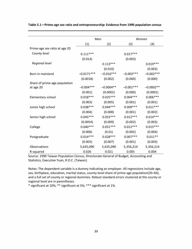
Using the 1990 population census, we regress the status of entrepreneurship on local sex ratios at the county or regional level and report the results in Table 5.1. A region is typically composed of two to four counties. Because demographic dividends have been regarded as a key driver of Taiwan’s economic growth (Bloom and Williamson 1998), we include as a control variable the share of prime-age population (20–64) corresponding to the year when an individual reaches age 20. To control for human capital, another widely viewed pinnacle of the Taiwan miracle (Lucas 1993; Stiglitz 1996), a set of dummy variables for educational levels (elementary school, junior high school, senior high school, college, and postgraduate) are included. In addition, a dummy variable for being born in the mainland, age, marital status, and a set of county fixed effects are added as controls.

[INSERT TABLE 5.1 ABOUT HERE]

Regardless of the sex ratio variable used, its coefficient is highly positive and statistically significant in regressions for men (Columns (1) and (2) in Table 5.1). The effect is economically significant—a 20 percent increase in the operational sex ratio boosts the

13

total percentage of men who become entrepreneurs by 2 percentage points. Given that only about 4 percent of men were reported to be entrepreneurs in the 1990 census, such an increase in sex ratios accounts for about 55.5 percent (0.2*0.111/0.04*100) of total entrepreneurial activities observed in 1990. In addition, the results are similar whether we use the county or regional sex ratio, suggesting that migration across counties should be less of a concern.

Interestingly, the sex ratio variable is also significant in the regressions for women (Columns (3) and (4) of Table 5.1), though the magnitude is much smaller (by a factor of 6) than for men. After women are married to small-business owners, some of the women get involved in the business and are naturally counted as entrepreneurs in the census. This is perhaps the main reason we also find a positive association between sex ratios and female entrepreneurship, rather than prediction by sexual selection.

The coefficient for the share of prime-age population is significantly negative, which does not support the population dividend hypothesis. All of the education dummy variables are positive and significant compared with the base of illiteracy. Interestingly, senior high school graduates are more likely to become entrepreneurs than are those with lower or higher levels of education.

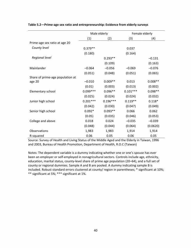
The census data suffer from a major limitation, as they ask the employment status at the time of the survey but do not inquire about employment history. Some people might have tried to be entrepreneurs, failed, and ended up working for others. Thus, they would be classified as nonentrepreneurs in the population census. To further explore the effect on entrepreneurial effort, we use an alternative dataset—the longitudinal Survey of Health and Living Status of the Middle Aged and the Elderly in Taiwan for 1996 and 2003. The survey enjoys a key advantage in that it contains detailed information on employment history.

About half of the women surveyed had never worked. Therefore, they are naturally defined as nonentrepreneurs. The survey’s entrepreneurship variable is subject to measurement errors, as also occurs in the population census. In the circumstance that both men and women worked, we cannot distinguish whether both of them were entrepreneurs or just one of them. Despite this caveat, the survey dataset is the only one available that allows us to separately examine men’s and women’s entrepreneurial effort in response to sex ratio imbalances by looking at their entire employment history.

The regression results for male and female elderly are reported in Table 5.2. Consistent with the sexual selection theory, men had a higher likelihood of trying entrepreneurial activities in their lives if they grew up in a region (or county) with more-skewed sex

14

ratios. The coefficients for the sex ratio variable are much larger than those observed in Table 5.1, roughly by a factor of 3. Considering that entrepreneurial activities are inherently risky and failure inevitably occurs, it is natural that the magnitude of the sex ratio variable in regressions on lifelong entrepreneurial effort is larger than that on current entrepreneurial status. In contrast to the significant coefficient in the male regressions, the sex ratio variable in female regressions is insignificant, as shown in Columns (3) and (4) of Table 5.2.

[TABLE 5.2 ABOUT HERE]

When county-level sex ratios are used, the share of prime-age population is insignificantly negative in the regression on male entrepreneurship. The variable becomes significantly positive when using regional sex ratios, in contrast to the results shown in Table 5.1. Overall, the results based on two different data sources provide mixed evidence on the population dividend hypothesis. Most of the education dummy variables are positive and significant, except for those for college graduates. Thus, there is not much difference between the chances of an illiterate person and a college-educated person becoming a entrepreneurs. Having some years of schooling, but not too many, however, improves the chance of entrepreneurship.

Sex Ratios and Labor Market Outcomes

In the marriage market, wealth is a crucial status variable. Becoming an entrepreneur is a quick means of accumulating wealth. Yet, it is not the only way. Even salaried men can increase their earnings by working longer hours. To investigate the importance of this channel, we use the Taiwan Manpower Utilization Survey of 1978, which includes information about employment status and working hours in the past week prior to the survey.

The survey was originally conducted monthly. However, the data we use are annual data, which pooled 12 monthly surveys from 1978 without any month indicator. The Manpower Utilization Survey used a sample rotation schedule, which meant that some households were surveyed multiple times in a year, while others were interviewed only once. The big challenge for us is that the households in the annual data lack unique identification. Based on enumeration area codes and household characteristics (such as household size, household head’s age, education level, and so on), however, we can uniquely identify all the household heads. For those surveyed more than once in a year, we randomly select one observation. In so doing, we create a cross-sectional household head dataset in which each household head has only one observation for 1978.

15

We mainly examine three outcome variables—having a job, weekly work hours, and being an entrepreneur. To make the household heads in the sample more comparable, we restrict the sample to male household heads between 20 and 50 years of age. The regression specifications follow Table 5.1 by including the prime-age sex ratio at the county level, the share of prime-age population (20–64) in the year the household head reached age 20, the household head age, ethnicity, education, marital status, and county fixed effects.

Panel A in Table 5.3 presents the regression results for the three outcome variables. The coefficients for the sex ratio variables in all three regressions are statistically significant and positive. An increase in prime-age sex ratio from 1 to 1.2 would boost the likelihood of holding a job by 7.3 percent (0.2*0.339/0.93*100), extend working hours by 7.8 percent (0.2*18.333/46.73*100), and enhance the chance of becoming an entrepreneur by 23.3 percent (0.2*0.07/0.06*100). These results suggest that mating competition enhances both extensive (more actively participating in the labor market and setting up more businesses) and intensive (putting forth greater work effect) margins of economic growth.

[INSERT TABLE 5.3 ABOUT HERE]

One may question that the cut-off age for household heads may be too high. By age 50, it is likely that some adult children have moved out of the household, making it less comparable with other younger, nuclear households. As a robustness check, we lower the household head age from 50 to 45 in Panel B and repeat the regressions outlined in Panel A. All of the coefficients remain highly significant, though the magnitude slightly declines as compared with Panel A.

In Panel C, we include households with at least two members, largely ruling out those bachelors who might behave differently from their married counterparts. The results are largely the same as in Panel A. All in all, mating competition induces families to more actively participate in the labor market, work longer hours, and engage in risky entrepreneurial activities.

16

Sex Ratios and Financial Outcomes

As men earn more, women might have the luxury of spending more lavishly if the number of men outstrips women in the marriage market. On the whole, it is not clear whether sex ratio imbalances are positively associated with household savings and wealth.

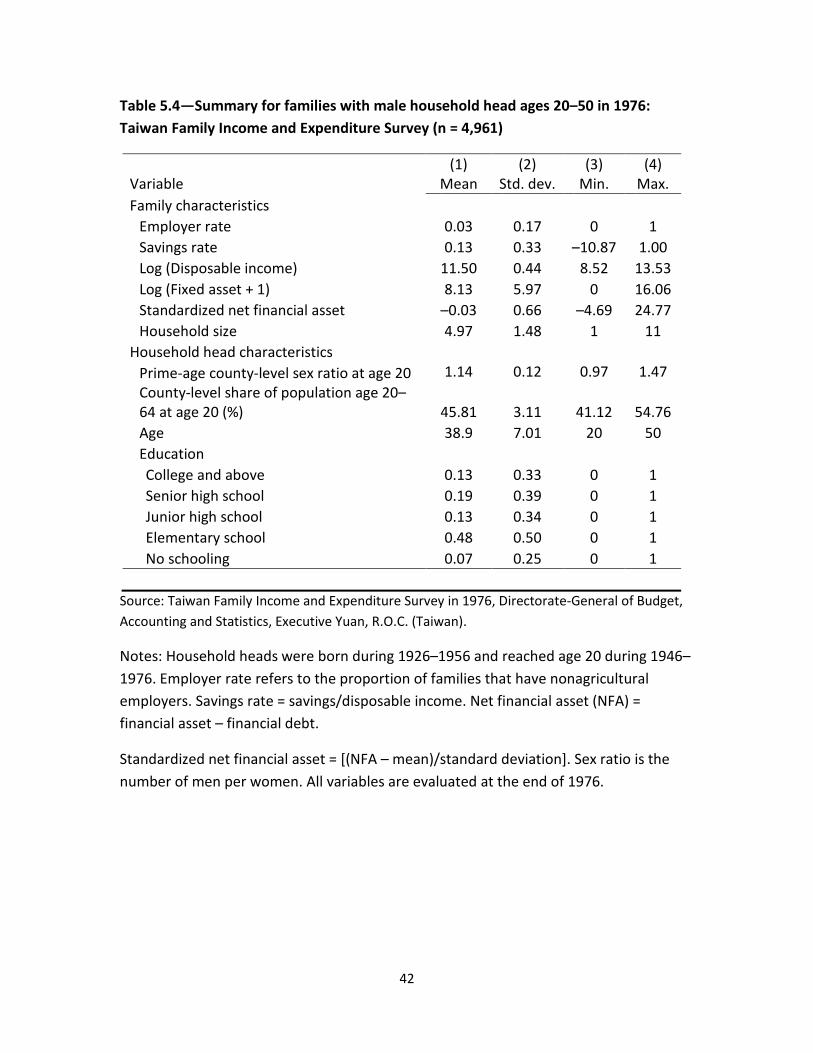
To empirically test the general equilibrium effect of sex ratio imbalances on household wealth, we make use of another dataset—the Taiwan Family Income and Expenditure Survey of 1976. This survey includes detailed information on household savings, fixed assets, and financial assets. We restrict the sample to include only nuclear families. As shown in the summary statistics in Table 5.4, the county-level sex ratio at age 20 was as high as 1.14, which is greater than that in the 1990 population census. This finding is consistent with the pattern depicted in Figure 3.1. The proportion of entrepreneurial households averages at 3 percent.

[INSERT TABLE 5.4 ABOUT HERE]

Table 5.5 presents the regression results based on the sample. We look at four outcome variables: entrepreneurship status, savings rate, fixed assets, and financial assets. Since a portion of households do not have any fixed assets, we use a Tobit regression. More specifically, we transform positive fixed asset values into logs and set the lower bound of the Tobit regressions as the smallest value minus a small positive number. Considering that the value of financial assets can be either positive or negative, we standardize it by subtracting the mean and dividing by the standard deviation.

[INSERT TABLE 5.5 ABOUT HERE]

In Panel A, we limit our sample to those nuclear households with male household heads between 20 and 50 years of age. As indicated in the first row, all four coefficients for the sex ratio variable are significantly positive. The regression result in Column (1) confirms the previous finding that sex ratio imbalances stimulate the competitive and risk-taking animal spirit of entrepreneurship. The result shown in Column (2) is consistent with Wei and Zhang (2011a), who found that household savings are positively associated with local sex ratios. A 20 percent increase in local sex ratios would increase the likelihood of becoming an entrepreneur by 73.3 percent (0.2*0.11/0.03*100) and boost the household savings rate by 46.2 percent (0.2*0.3/0.13*100), which are both economically significant. The marginal effect on fixed assets is 15.1 percent (0.2*6.12/8.13*100). When discussing Taiwan’s economic miracle, Stiglitz (1996) regarded high savings rates as a motor of growth. He emphasized the role of government in mobilizing savings. Note that the literature has never mentioned mating

17

competition as a driver behind Taiwan’s high savings rates. Finally, Column (4) presents the results on financial assets. The coefficient for the sex ratio variable is also statistically significant, suggesting that the marriage market squeeze induces families to amass financial assets.

One may be concerned about the sensitivity of the results in relation to the cut-off age of the household head. As a robustness check, we restrict the sample to the households with male household heads no older than 45 and repeat the analysis in Panel B. The main results—that mating competition shapes human economic behavior—are intact. The samples used in Panels A and B include households regardless of their marriage and child status, though household size is controlled. However, there is a possibility that households with children might behave quite differently from those that are childless. Likewise, married households could differ greatly from singles. In Panel C, we drop bachelors from the sample used in Panel A and follow the same specification. All of the results carry through.

The General Equilibrium Effect

We have shown so far that in the wake of adverse terms of trade in the marriage market, men tend to take risky entrepreneurial activities, save more, and accumulate more wealth. Since these factors are the key ingredients for economic growth, we conjecture that mating competition might well contribute to Taiwan’s economic growth. To check this possibility, Figure 5.2 plots the sex ratio and the five-year moving average of real gross domestic product (GDP) growth rate over more than half a century. The two lines in the figure largely follow the same pattern though the dashed line for GDP is more erratic, suggesting a positive relationship between mating competition and economic growth. We recognize that this is only suggestive evidence and that there might be some unobservable factors that affect both the trend of sex ratios and the pattern of economic growth over time. However, the unobserved factors are less likely to be omnipresent in all regions all the time.

[INSERT FIGURE 5.2 ABOUT HERE]

In Figure 5.3, we plot the extensive enterprise growth rates in three periods (1954–1961, 1961–1966, and 1966–1971) against the initial prime-age sex ratio in each period at the county level by controlling for period fixed effects.10 The figure reveals that there was a

10 The Industry and Commerce Census was first conducted in 1954. The second census was undertaken in 1961. Thereafter, the census has been repeated every five years. Since the operation sex ratios are imputed at the county level and the number of registered enterprises is also at the county level, we do not control for county fixed effects in the conditional plot.

18

large regional variation in prime-age sex ratios in the 1950s and 1960s. The slope of the fitted line is 37 and is statistically significant with a t-value of 2.8. This result indicates a positive relation between extensive enterprise growth and sex ratio imbalances. More specifically, a 20 percent increase in prime-age sex ratio would boost the growth in the number of enterprises by 7.4 percentage points (0.2*37%). Given that the extensive enterprise growth rate across the three periods averaged 27.5 percent, such a contribution resulting from an increase in sex ratio imbalances is economically significant.

[INSERT FIGURE 5.3 ABOUT HERE]

Theoretically, in a closed economy, increases in savings rates induced by mating competition may create a domestic economic imbalance of overinvestment and underconsumption. This, in turn, would depress the prices of domestic industrial products and make long-term economic growth unsustainable. In practice, Taiwan has been an open economy from the beginning. The excess output owing to mating competition is absorbed by consumers in other countries through international trade. Figure 5.4 graphs the time series of export growth rate from the mid-1950s to 2010, which mirrors the temporal pattern of sex ratios. Once again, this tentative evidence suggests that some macroeconomic outcomes, such as export performance, may have a biological origin.

[INSERT TABLE 5.4 ABOUT HERE]

Potential Alternative Explanations

Although we find a positive association between operational sex ratios and the prevalence of entrepreneurship across regions, the impact may not solely come from the channel of mating competition. There are at least five alternative channels. First, when the Kuomintang army fled to Taiwan, it brought a significant amount of treasures. Areas with higher sex ratios frequently happened to have military bases. As a result, those areas likely received more financial transfers from the government or even bilateral military aid from the United States. As the military spent the money, it stimulated local businesses and created jobs. We argue that this effect, if it even was an effect, has already been controlled for in our analyses. The spatial distribution of military bases and government institutions had barely changed from the 1950s to the early 1980s. In addition, most of the military and government reform did not occur until Chiang Kai-shek passed away in 1975. Since our analysis primarily focuses on the period before that, the number of military and government institutions in a region can be largely treated as fixed. Technically, the influence of these institutions on the local

19

economy can be largely controlled by the inclusion of county fixed effects in all regressions. Moreover, their presence alone could not explain the bell-shaped temporal pattern of the extensive firm growth.

Second, as the soldiers who retreated from mainland China aged and retired from the military, they needed to find jobs in the civilian sectors. Given their limited education and working experience, they might have had difficulty finding formal jobs and were forced to become self-employed or start small businesses in local areas. In other words, they had no choice but to become entrepreneurs, which has nothing to do with mating competition. However, even if veterans ended up as entrepreneurs in a larger proportion for reasons unrelated to sex ratio imbalances, the overall effect would be rather muted because of their small size. As shown in Table 4.3, mainlanders account for only 6 percent of the elderly sample. To check the robustness of our results to this potential effect, we drop the mainlanders from the sample and repeat the regressions on the restricted sample (see Tables 5.1 and 5.2).11 All of the main results remain largely the same.

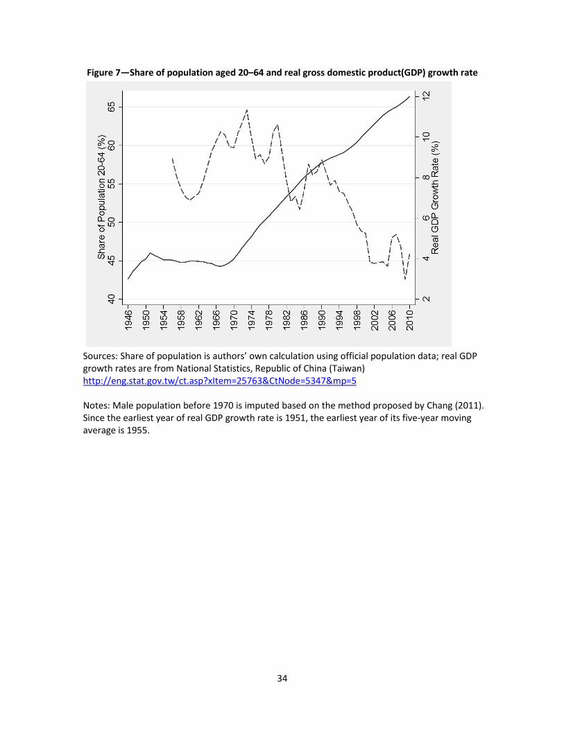
Third, most soldiers and civilians who fled from the mainland were in their prime working age in the 1950s and 1960s, thus creating an extremely favorable low dependency ratio (that is, the ratio of prime working age population to the population over 60 years old). If areas with high operational sex ratios also happened to have a large share of prime-age workers, the observed impact of sex ratios may actually capture the impact of the population dividend with a high fraction of the working-age population. In fact, in all of the regressions, we include the share of prime-age population at the county level. Even so, we find a positive association between mating competition and male entrepreneurship after controlling for the share of prime-age population. Moreover, when we plot the share of prime-age population versus real export or GDP growth rates in the same figure, it appears that the pattern of the share of prime-age population bears little resemblance to those of the two key economic variables (see Figures 5.2 and 5.3).

Fourth, it is likely that higher sex ratios represent some omitted variables, such as growth opportunities, which also happen to be related to entrepreneurship. When Kuomintang retreated to Taiwan, they set up their military bases mainly for the strategic purpose of defense, without taking economic growth into consideration. Local sex ratios are highly correlated with the presence of military bases, which are largely invariable over time. By including county fixed effects, we can, to a large degree, control for

11 The results are not presented here but are available upon request.

20

(though hardly eliminate) the unobserved, location-specific factors related to growth potentials.

Fifth, if men in counties with skewed sex ratios can easily marry women in counties with more normal sex ratios, then the operational sex ratio may not measure the true degree of marriage market squeeze. Such a measurement error may cloud a precise estimation of the true impact. To ameliorate the concern, in all of the regressions, we also check the robustness of the results by replacing sex ratios at the county level with ones at the more aggregate regional level. In theory, the incidence of cross-regional marriage must be lower than that across counties, because a region encompasses multiple counties. Our results remain largely the same when using regional sex ratios. In effect, most marriages prior to the 1980s occurred at the local level.

21

6. Conclusions

From a Darwinian perspective, the struggle for reproduction is a marker for any species, including human beings. Failure to find a mate is a dreadful fate for humankind. Because wealth is a crucial status indicator in the human marriage market, men tend to intensify their effort to pursue wealth when the terms of trade favor women. Since being an entrepreneur is perhaps a readily available way for one to get rich, we hypothesize that increasing the ratio of males to females induces more men of marriageable age to initiate entrepreneurial activities, despite the inherently high risk. The unintended marriage market squeeze that originated from the Kuomintang army’s retreat to Taiwan provides us with a natural experiment to directly test this hypothesis, a key insight drawn from the evolutionary biology literature.

Using four different datasets, we reach the same finding: that mating competition triggers men’s entrepreneurship. As illustrated in this paper, the demographic shocks in the late 1940s caused by the injection of a massive number of young men onto the island sparked men’s entrepreneurship, which in turn contributed to Taiwan’s economic miracle in subsequent decades. To our knowledge, no one has delineated Taiwan’s economic miracle from this Darwinian perspective. Thus, the Darwinian perspective on sexual selection offers a new lens for looking at human economic behavior and aggregate economic outcomes.

We end the paper on a cautious note. Our finding on the positive association between sex ratios and entrepreneurship does not mean that governments should promote economic growth by purposely manipulating imbalanced sex ratios. For one thing, the government does not have the moral ground to abort any babies on behalf of individuals. In addition, as shown by the large body of literature, imbalanced sex ratios can result in serious social ills (Edlund et al., 2007; Ebenstein, 2010). The key objective of our paper is to demonstrate that some aspects of human economic behavior might have a biological root. Fusing a biological perspective with economic analysis can shed new insight on human economic behaviors and outcomes.

22

References

Angrist, Joshua, 2002, “How Do Sex Ratios Affect Marriage and Labor Markets? Evidence

from America’s Second Generation,” Quarterly Journal of Economics, 117 (3):

997-1038.

Barclay, G. W. 1954. Colonial Development and Population in Taiwan. New Jersey:

Princeton University Press.

Becker, Gary S.1981. A Treatise on the Family. Harvard University Press. Cambridge.

Bloom, D. E., and J. G. Williamson. 1998. “Demographic Transition and Economic

Miracles in Emerging Asia.” World Bank Economic Review 12 (3): 419–455.

Brown, P. H., E. Bulte, and X. Zhang. 2011. “Positional Spending and Status Seeking in

Rural China.” Journal of Development Economics 96 (1): 139–149.

Bulte, E., N. Heerink, and X. Zhang. 2011. “China’s One-Child Policy and ‘the Mystery of

Missing Women: Ethnic Minorities and Male-Biased Sex Ratios.” Oxford Bulletin

of Economics and Statistics 73 (1): 21–39.

Buss, D. M. 1989. Sex Differences in Human Mater Preferences: Evolutionary Hypothesis

Tested in 37 Countries. Behavioural and Brain Sciences 12 (1): 1–49.

Bureau of Health Promotion, Department of Health, R.O.C (Taiwan). Various years.

Longitudinal Survey of Health and Living Status of the Middle-aged and the

Elderly in Taiwan.

Chang, S. 2011. Civil War, Marriage Ban, and Sex Ratio: Impute the Prime-age Sex Ratio

in Post-War Taiwan Using Censored Data. China Center for Human Capital and

Labor Market Research, no. 34. Beijing: CHLR.

Chen, K. J., and T. F. Yeh. 1982. “Changes of Age Composition in Taiwan, 1905–1979.”

National Taiwan University Journal of Population Studies 6:99–114.

Cole, Harold L., George J. Mailath, and Andrew Postlewaite, 1992, “Social Norms,

Savings Behavior, and Growth.” Journal of Political Economy, 100(6): 1092-

1125.Cox, D. 2007. “Biological Basics and the Economics of the Family.” Journal

of Economic Perspective 21 (2): 91–108.

23

Darwin, C. 1871. The Descent of Man and Selection in Relation to Sex. London: John

Murray.

Das Gupta, M. 2005. “Explaining Asia’s Missing Women.” Population and Development

Review 31:529–535.

Den Boer, A., and V. M. Hudson. 2004. “The Security Threat of Asia’s Sex Ratios.” SAIA

Review 24(2): 27–43.

,Directorate-General of Budget, Accounting and Statistics, Executive Yuan, R.O.C.

(Taiwan). Various years. The Industry and Commerce Census of Taiwan.

________. 1990. Taiwan Population Census

Du, Q., and S.-J. Wei. 2011. Sex Ratios and Entrepreneurship. working paper, Columbia

University Business School. New York: Columbia University.

Ebenstein, A. 2010. “The ‘Missing Girls’ of China and the Unintended Consequences of

the One Child Policy.” Journal of Human Resources 45 (1): 87–115.

Edlund, L. 2000. “The Marriage Squeeze Interpretation of Dowry Inflation: A Comment.”

Journal of Political Economy 108:1327–1333.

Edlund, L., H. Li, J. Yi, and J. Zhang. 2007. Sex Ratios and Crime: Evidence from China’s

One-Child Policy. IZA Discussion Paper, no. 3214, Bonn, Germany.

Francis, A. 2011. “Sex Ratios and the Red Dragon: Using the Chinese Communist

Revolution to Export the Effect of the Sex Ration on Women and Children in

Taiwan.” Journal of Population Economics, 24: 813-837

Frank, R. H. 1985. “The Demand for Unobservable and Other Nonpositional Goods.”

American Economic Review 75 (1): 101–116.

________. 2004. “Positional Externalities Cause Large and Preventable Welfare Losses.”

American Economic Review 95 (2): 137–141.

________. 2007. Falling Behind: How Rising Inequality Hurts the Middle Class? Berkeley:

University of California Press.

________. 2011. The Darwin Economy: Liberty, Competition, and the Common Good.

New Jersey: Princeton University Press.

24

Griskevicius, Vladas, Joshua M. Tybur, Joshua M. Ackerman, Andrew W. Delton, and

Theresa E. Robertson. 2012. “The Financial Consequences of Two Many Men: Sex

Ratio Effects on Saving, Borrowing and Spending.” Journal of Personality and

Social Psychology, 102 (1): 69-80.

Ho, S. P. S. 1978. Economic Development of Taiwan: 1860–1970. New Haven: Yale

University Press.

Hopkins, E., and T. Kornienko. 2010. “Which Inequality? The Inequality of Endowments

versus the Inequality of Rewards.” American Economic Journal: Microeconomics,

2 (3): 106–137.

Jacoby, N. H. 1967. U.S. Aid to Taiwan: A Study of Foreign Aid, Self-Help, and

Development. New York: F. A. Praeger.

Li, H., and H. Zheng. 2009. “Ultrasonography and Sex Ratios in China” Asian Economic

Policy Review 4 (1): 121–137.

Lin, S. W. 2002. “The Transition of Demographic Sexual Structure in Taiwan: 1905–2000.”

National Chengchi University Journal of Sociology 33:91–131.

Liu, K. C. 1986. Population Growth and Economic Development in Taiwan. Taipei: Linking

Books.

Lucas, R. E. 1993. “Making a Miracle.” Econometrica 61 (2): 251–272.

Ministry of Interior, Taiwan. Various years. Taiwan Demographic Fact Books. See

http://eng.stat.gov.tw/ct.asp?xItem=25763&CtNode=5347&mp=5.

Nettle, Daniel and Thomas V. Pollet. 2008. “Natural Selection and Male Wealth in

Humans.” American Naturalist, 172 (5): 813-837.

Porter, Maria. 2011. “Intra-Household Bargaining and Support of Elderly Parents in

China.” Working paper. University of Oxford.

Qian, N. 2008. “Missing Women and the Price of Tea in China: The Effect of Sex-specific

Earnings on Sex Imbalance.” Quarterly Journal of Economics 123 (3): 1251–1285.

Rao, V. 1993. “The Rising Price of Husbands: A Hedonic Analysis of Dowry Increases in

Rural India.” Journal of Political Economy 101:666–677.

25

Robson, A. J. 1992. “Status, the Distribution of Wealth, Private and Social Attitudes to

Risk.” Econometrica 60 (4): 837–857.

Stiglitz, J. E. 1996. “Some Lessons from the East Asia Miracle.” World Bank Research

Observer 11 (2): 151–177.

Trivers, R. L., and D. E. Willard. 1973. “Natural Selection of Parental Ability to Vary the

Sex Ratio of Offspring.” Science 179:90–92.

Wei, S.-J., and X. Zhang. 2011a. “The Competitive Saving Motive: Evidence from Rising

Sex Ratios and Savings Rates in China.” Journal of Political Economy 119 (3): 511–

564.

________. 2011b. Sex Ratios, Entrepreneurship, and Economic Growth in the People’s

Republic of China. National Bureau of Economic Research Working Paper, no.

16800. Cambridge, MA: NBER.

26

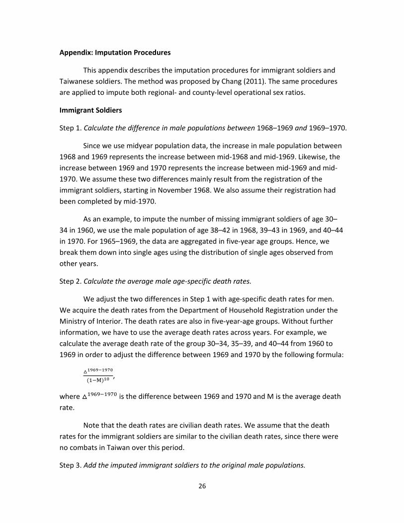
Appendix: Imputation Procedures

This appendix describes the imputation procedures for immigrant soldiers and Taiwanese soldiers. The method was proposed by Chang (2011). The same procedures are applied to impute both regional- and county-level operational sex ratios.

Immigrant Soldiers

Step 1. Calculate the difference in male populations between 1968–1969 and 1969–1970.

Since we use midyear population data, the increase in male population between 1968 and 1969 represents the increase between mid-1968 and mid-1969. Likewise, the increase between 1969 and 1970 represents the increase between mid-1969 and mid-1970. We assume these two differences mainly result from the registration of the immigrant soldiers, starting in November 1968. We also assume their registration had been completed by mid-1970.

As an example, to impute the number of missing immigrant soldiers of age 30–34 in 1960, we use the male population of age 38–42 in 1968, 39–43 in 1969, and 40–44 in 1970. For 1965–1969, the data are aggregated in five-year age groups. Hence, we break them down into single ages using the distribution of single ages observed from other years.

Step 2. Calculate the average male age-specific death rates.

We adjust the two differences in Step 1 with age-specific death rates for men. We acquire the death rates from the Department of Household Registration under the Ministry of Interior. The death rates are also in five-year-age groups. Without further information, we have to use the average death rates across years. For example, we calculate the average death rate of the group 30–34, 35–39, and 40–44 from 1960 to 1969 in order to adjust the difference between 1969 and 1970 by the following formula:

△1969−1970

(1−M)10,

where △1969−1970 is the difference between 1969 and 1970 and M is the average death rate.

Note that the death rates are civilian death rates. We assume that the death rates for the immigrant soldiers are similar to the civilian death rates, since there were no combats in Taiwan over this period.

Step 3. Add the imputed immigrant soldiers to the original male populations.

27

As the last step, we add the adjusted differences to the original male population in 1960. For the immigrant soldiers, we impute for the group of age 30–34 from 1960–1964, the group of age 35–39, 40–44, and 45–49 from 1960–1969. When impute backwardly, these are the age-year cells that are affected.

Taiwanese Soldiers

To impute the Taiwanese soldiers, we simply fit a linear projection between 1954 and 1965 for the age group 20–24. Taiwanese soldiers mostly serve in their early twenties for two to three years, so they do not affect other age groups. Meanwhile, men and women of this age group parallel to each other except for the period 1955–1964 and the women population appears to be linear over this period. Therefore, it is reasonable to assume that the men population should also be linear, were the Taiwanese soldiers not excluded.

28

Figure 3.1—Prime-age sex ratio and women marriage rate

Sources: Prime-age sex ratio is derived from the authors’ own calculation; women marriage rates are from various Taiwan Demographic Fact Books published by Ministry of Interior, Taiwan. See http://eng.stat.gov.tw/ct.asp?xItem=25763&CtNode=5347&mp=5. Notes: Prime-age sex ratio is defined as the number of men per women for ages 15–49; marriage rate is the percentage of married women among all women who are at least 15 years old.

29

Figure 5.1—Prime-age sex ratio and growth rate of number of registered companies

Sources: Prime-age sex ratio is authors’ own calculation; registered company data are from Ministry of Economic Affairs (MOEA), Taiwan. Notes: Prime-age sex ratio is defined as the number of men per women for age 15–49. A registered company refers to a corporate legal entity organized or incorporated in accordance with the Company Act in Taiwan. Since the earliest year for number of registered company is 1951, the earliest year of its five-year moving average of growth rate is 1956.

30

Figure 5.2—Prime-age sex ratio and real gross domestic product growth (GDP)rate

Sources: Prime-age sex ratio is from the authors’ own calculation. Real GDP growth rates are from National Statistics, Republic of China (Taiwan) http://eng.stat.gov.tw/ct.asp?xItem=25763&CtNode=5347&mp=5. Notes: Prime-age sex ratio is defined as the number of men per women ages 15–49. Since the earliest year of real GDP growth rate is 1951, the earliest year of its five-year moving average is 1955.

31

Figure 5.3—Partial regression of extensive enterprise growth rate on prime-age sex ratio

Sources: Prime-age sex ratios are from the authors’ imputation. Numbers of enterprises are acquired from the Industry and Commerce Census of Taiwan in 1954, 1961, 1966, and 1971,Directorate-General of Budget, Accounting and Statistics, Executive Yuan, R.O.C. (Taiwan). Note: Each dot represents a pair of residual in prime-age sex ratio at the baseline year of three periods (1954–1961, 1961–1966, and 1966–1971) and residual in the growth rate of the number of enterprises over the respective period in each county. The residuals are obtained from regressions of prime-age sex ratio and enterprise growth rate on period fixed effects. The coefficient and robust standard error of the fitted regression line are reported at the bottom.

32

Figure 5.4—Prime-age sex ratio and real export growth rate

Sources: Prime-age sex ratio is from the authors’ own calculation. Real export growth rates are from National Statistics, Republic of China (Taiwan) http://eng.stat.gov.tw/ct.asp?xItem=25763&CtNode=5347&mp=5.

Notes: Prime-age sex ratio is defined as the number of men per women ages 15–49. Since the earliest year of real export growth rate is 1952, the earliest year of its five-year moving average is 1956.

33

Figure 6—Share of population aged 20–64 and real export growth rate

Sources: Share of population is authors’ own calculation using official population data; real export growth rates are from National Statistics, Republic of China (Taiwan) http://eng.stat.gov.tw/ct.asp?xItem=25763&CtNode=5347&mp=5 Notes: Male population before 1970 is imputed based on the method proposed by Chang (2011). Since the earliest year of real export growth rate is 1952, the earliest year of its five-year moving average is 1956.

34

Figure 7—Share of population aged 20–64 and real gross domestic product(GDP) growth rate

Sources: Share of population is authors’ own calculation using official population data; real GDP growth rates are from National Statistics, Republic of China (Taiwan) http://eng.stat.gov.tw/ct.asp?xItem=25763&CtNode=5347&mp=5 Notes: Male population before 1970 is imputed based on the method proposed by Chang (2011). Since the earliest year of real GDP growth rate is 1951, the earliest year of its five-year moving average is 1955.

35

Table 4.1—Summary of men and women aged 20–59 in the 1990 population census (aged 20 during 1951–1990)

Men (n = 5,635,090)

Women (n = 5,356,214)

(1) (2) (3) (4) Mean Std. dev. Mean Std. dev. Employer 0.04 0.20 0.01 0.09 Prime-age sex ratio at age 20

County level 1.10 0.09 1.10 0.09 Regional level 1.10 0.08 1.10 0.08

Age 35.46 10.78 35.49 10.71 Birthplace/Ancestral home

Taiwan 0.88 0.32 0.86 0.34 Mainland China 0.12 0.32 0.14 0.34 Other countries 0.00 0.04 0.00 0.04

Education No formal education 0.03 0.16 0.09 0.29 Elementary school 0.26 0.44 0.32 0.47 Junior high school 0.20 0.40 0.17 0.37 Senior high school 0.29 0.46 0.27 0.45 College 0.21 0.41 0.14 0.35 Postgraduate 0.01 0.11 0.00 0.07

Marital status Single 0.34 0.47 0.22 0.42 Married 0.63 0.48 0.72 0.45 Divorced 0.02 0.14 0.02 0.15 Widowed 0.01 0.09 0.03 0.17

Source: Taiwan 1990 Population Census ,Directorate-General of Budget, Accounting and Statistics, Executive Yuan, R.O.C. (Taiwan).

Notes: Prime-age sex ratio is defined as the number of men per women for ages 15–49. All variables are evaluated on December 16, 1990, except for the prime-age sex ratios.

36

Table 4.2—Are employers more likely to be married?

Men (1)

Women (3)

Employer 0.145*** –0.003 (0.006) (0.009) Elementary school 0.227*** 0.153*** (0.006) (0.009) High school 0.278*** 0.104*** (0.008) (0.020) College and above 0.249*** –0.081* (0.015) (0.043) Observations 5,635,090 5,356,214 R-squared 0.32 0.18 Source: Taiwan 1990 Population Census, Directorate-General of Budget, Accounting and Statistics, Executive Yuan, R.O.C. (Taiwan). Notes: The dependent variable is a dummy variable indicating being married if the value is 1. Employer is a dummy variable indicating being an employer. The reference education group is no education. High school includes both junior and senior high. Both regressions include age, birthplace, and a full set of county dummies. Robust standard errors clustered at the county level are in parentheses. * significant at 10%; ** significant at 5%; *** significant at 1%. Table 4.3—Summary of two elderly samples

Sample A: 1930–1945 (n = 2,298)

Sample B: 1946–1953 (n = 1,599)

(1) (2) (3) (4) Mean Std. dev. Mean Std. dev. One spouse has ever been

employer/self-employed 0.22 0.42 0.31 0.46

Has at least one biological child ever born 0.97 0.18 0.94 0.23

Total of biological children ever born 3.91 1.67 2.83 1.28

Prime-age sex ratio at age 20 County level 1.14 0.11 1.17 0.05 Regional level 1.13 0.09 1.16 0.04

Age in 1996 57.35 4.44 46.36 2.01 Male 0.51 0.50 0.51 0.50 Ethnicity

Minnan 0.75 0.43 0.75 0.43 Hakka 0.17 0.38 0.17 0.38 Mainlander 0.06 0.24 0.05 0.22

37

Other ethnic group 0.02 0.12 0.02 0.14 Education

No formal education 0.29 0.45 0.04 0.21 Elementary school 0.47 0.50 0.47 0.50 Junior high school 0.10 0.30 0.14 0.35 Senior high school 0.08 0.28 0.18 0.39 College and above 0.06 0.23 0.15 0.36

Marital status Single 0.02 0.14 0.04 0.19 Married 0.84 0.37 0.83 0.38 Divorced 0.03 0.17 0.06 0.24 Widowed 0.11 0.31 0.07 0.25

Source: Longitudinal Survey of Health and Living Status of the Middle-aged and the Elderly in Taiwan 1996 and 2003, Bureau of Health Promotion, Department of Health, R.O.C (Taiwan) Notes: Sample A was drawn in 1996 to represent the elderly population aged 51–66 in 1996. Sample B was drawn in 2003 to represent the elderly population aged 50–57 in 2003. Therefore, variables are evaluated in 1996 for Sample A and in 2003 for Sample B. However, for comparison, age is evaluated in 1996 for both. The variable in the first row is a dummy variable equal to 1 if either one or one’s spouse has ever been an employer or self-employed in the nonagricultural sector up to the point of interview. This variable is constructed from an original survey question that asks who the owner of one’s firm is. However, if one or one’s spouse is the owner, the survey does not further distinguish the two.

Table 4.4—Are entrepreneurs more likely to have children? Evidence from elderly surveys

(1) Male elderly (n = 1,983)

(2) Female elderly

(n = 1,914) Panel A: Have at least one biological child born One spouse has ever been

employer/self-employed 0.017*** 0.002 (0.005) (0.006)

R-squared 0.13 0.12 Panel B: Total of biological children born One spouse has ever been

employer/self-employed 0.034 –0.197***

(0.079) (0.064) R-squared 0.39 0.3080

Source: Longitudinal Survey of Health and Living Status of the Middle-aged and the Elderly in Taiwan 1996 and 2003, Bureau of Health Promotion, Department of Health, R.O.C (Taiwan) Notes: Dependent variables include both alive and deceased biological children. Controls include age, ethnicity, education, marital status, and a full set of county dummies. Samples A and B are pooled. A dummy indicating Sample B is included. Robust standard errors clustered at the county level are in parentheses. * significant at 10%; ** significant at 5%; *** significant at 1%.

38

39

Table 5.1—Prime-age sex ratio and entrepreneurship: Evidence from 1990 population census

Men Women (1) (2) (3) (4) Prime-age sex ratio at age 20

County level 0.111*** 0.017*** (0.014) (0.003)

Regional level 0.113*** 0.019*** (0.010) (0.003)

Born in mainland –0.0171*** –0.016*** –0.003*** –0.002*** (0.0018) (0.002) (0.000) (0.000) Share of prime-age population at age 20 –0.004*** –0.0004** –0.001*** –0.0002** (0.001) (0.0002) (0.000) (0.0001) Elementary school 0.018*** 0.025*** 0.004*** 0.006*** (0.003) (0.005) (0.001) (0.001) Junior high school 0.038*** 0.044*** 0.009*** 0.011*** (0.004) (0.008) (0.001) (0.002) Senior high school 0.045*** 0.053*** 0.012*** 0.014*** (0.0054) (0.009) (0.002) (0.003) College 0.040*** 0.051*** 0.012*** 0.015*** (0.006) (0.01) (0.002) (0.004) Postgraduate 0.014*** 0.028*** 0.007*** 0.011** (0.003) (0.007) (0.001) (0.003) Observations 5,635,090 5,635,090 5,356,214 5,356,214 R-squared 0.026 0.021 0.005 0.004

Source: 1990 Taiwan Population Census, Directorate-General of Budget, Accounting and Statistics, Executive Yuan, R.O.C. (Taiwan). Notes: The dependent variable is a dummy indicating an employer. All regressions include age, sex, birthplace, education, marital status, county-level share of prime-age population(20–64), and a full set of county or regional dummies. Robust standard errors clustered at the county or regional level are in parentheses. * significant at 10%; ** significant at 5%; *** significant at 1%.

40

Table 5.2—Prime-age sex ratio and entrepreneurship: Evidence from elderly surveys

Male elderly Female elderly (1) (2) (3) (4) Prime-age sex ratio at age 20

County level 0.379** 0.037 (0.180) (0.164)

Regional level 0.293** –0.131 (0.109) (0.163)

Mainlander –0.064 –0.056 –0.069 –0.076 (0.051) (0.048) (0.051) (0.065) Share of prime-age population at age 20 –0.010 0.009** 0.013 0.008** (0.01) (0.003) (0.013) (0.002) Elementary school 0.099*** 0.096** 0.101*** 0.098** (0.025) (0.024) (0.024) (0.032) Junior high school 0.201*** 0.196*** 0.119** 0.118* (0.042) (0.030) (0.047) (0.049) Senior high school 0.092* 0.093** 0.066 0.062 (0.05) (0.035) (0.046) (0.053) College and above 0.018 0.024 –0.035 –0.039 (0.048) (0.044) (0.064) (0.0620) Observations 1,983 1,983 1,914 1,914 R-squared 0.06 0.05 0.06 0.05

Source: Survey of Health and Living Status of the Middle Aged and the Elderly in Taiwan, 1996 and 2003, Bureau of Health Promotion, Department of Health, R.O.C (Taiwan) Notes: The dependent variable is a dummy indicating whether one or one’s spouse has ever been an employer or self-employed in nonagricultural sectors. Controls include age, ethnicity, education, marital status, county-level share of prime age population (20–64), and a full set of county or regional dummies. Sample A and B are pooled. A dummy indicating sample B is included. Robust standard errors clustered at county/ region in parentheses; * significant at 10%; ** significant at 5%; *** significant at 1%.

41

Table 5.3—Prime-age sex ratio and labor market outcomes: Evidence from Taiwan Manpower Survey

(1) Have a job

(mean = 0.93)

(2) Weekly work hours

(mean = 46.73)

(3) Employer rate (mean = 0.06)

Panel A: Male household head aged 20–50 Prime-age sex ratio at age 20 0.339*** 18.333*** 0.070** (0.032) (2.029) (0.027) Observation 49,509 49,509 49,509 R-squared 0.09 0.09 0.03 Panel B: Male household head aged 20–45 Prime-age sex ratio at age 20 0.201*** 11.601*** 0.050** (0.028) (1.941) (0.023) Observation 36,833 36,833 36,833 R-squared 0.10 0.09 0.03

Panel C: Male household head aged 20–50 with at least two

household members Prime-age sex ratio at age 20 0.320*** 18.664*** 0.067** (0.029) (2.110) (0.025) Observation 45,155 45,155 45,155 R-squared 0.06 0.07 0.03

Source: Taiwan Manpower Survey in 1978, Directorate-General of Budget, Accounting and Statistics, Executive Yuan, R.O.C. (Taiwan) Notes: Prime-age sex ratio (the number of men per women) is at the county level. Male household heads were born between 1928 and 1958 and reached age 20 between 1948 and 1978. All regressions control for household head’s age, marital status, education, household size, county-level share of prime age (20–64) population at age 20, and a full set of county dummies. Robust standard errors clustered at the county level are in parentheses. * significant at 10%; ** significant at 5%; *** significant at 1%.

42

Table 5.4—Summary for families with male household head ages 20–50 in 1976: Taiwan Family Income and Expenditure Survey (n = 4,961)

Variable (1)

Mean (2)

Std. dev. (3)

Min. (4)

Max. Family characteristics

Employer rate 0.03 0.17 0 1 Savings rate 0.13 0.33 –10.87 1.00 Log (Disposable income) 11.50 0.44 8.52 13.53 Log (Fixed asset + 1) 8.13 5.97 0 16.06 Standardized net financial asset –0.03 0.66 –4.69 24.77 Household size 4.97 1.48 1 11

Household head characteristics Prime-age county-level sex ratio at age 20 1.14 0.12 0.97 1.47 County-level share of population age 20–64 at age 20 (%) 45.81 3.11 41.12 54.76 Age 38.9 7.01 20 50 Education College and above 0.13 0.33 0 1 Senior high school 0.19 0.39 0 1 Junior high school 0.13 0.34 0 1 Elementary school 0.48 0.50 0 1 No schooling 0.07 0.25 0 1

Source: Taiwan Family Income and Expenditure Survey in 1976, Directorate-General of Budget, Accounting and Statistics, Executive Yuan, R.O.C. (Taiwan).

Notes: Household heads were born during 1926–1956 and reached age 20 during 1946–1976. Employer rate refers to the proportion of families that have nonagricultural employers. Savings rate = savings/disposable income. Net financial asset (NFA) = financial asset – financial debt.

Standardized net financial asset = [(NFA – mean)/standard deviation]. Sex ratio is the number of men per women. All variables are evaluated at the end of 1976.

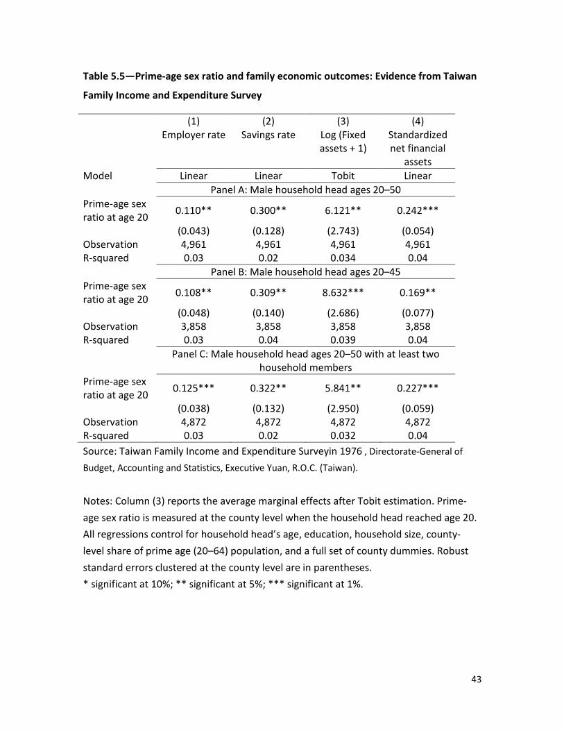
43

Table 5.5—Prime-age sex ratio and family economic outcomes: Evidence from Taiwan

Family Income and Expenditure Survey

(1) Employer rate

(2) Savings rate

(3) Log (Fixed assets + 1)

(4) Standardized net financial

assets Model Linear Linear Tobit Linear

Panel A: Male household head ages 20–50 Prime-age sex ratio at age 20 0.110** 0.300** 6.121** 0.242***

(0.043) (0.128) (2.743) (0.054) Observation 4,961 4,961 4,961 4,961 R-squared 0.03 0.02 0.034 0.04

Panel B: Male household head ages 20–45 Prime-age sex ratio at age 20 0.108** 0.309** 8.632*** 0.169**

(0.048) (0.140) (2.686) (0.077) Observation 3,858 3,858 3,858 3,858 R-squared 0.03 0.04 0.039 0.04

Panel C: Male household head ages 20–50 with at least two household members

Prime-age sex ratio at age 20 0.125*** 0.322** 5.841** 0.227***

(0.038) (0.132) (2.950) (0.059) Observation 4,872 4,872 4,872 4,872 R-squared 0.03 0.02 0.032 0.04 Source: Taiwan Family Income and Expenditure Surveyin 1976 , Directorate-General of

Budget, Accounting and Statistics, Executive Yuan, R.O.C. (Taiwan). Notes: Column (3) reports the average marginal effects after Tobit estimation. Prime-age sex ratio is measured at the county level when the household head reached age 20. All regressions control for household head’s age, education, household size, county-level share of prime age (20–64) population, and a full set of county dummies. Robust standard errors clustered at the county level are in parentheses. * significant at 10%; ** significant at 5%; *** significant at 1%.