The Economic Consequences of Colorism and Complexion Homogamy in the Black Community:

Some Historical Evidence

Howard Bodenhorn Department of Economics

Lafayette College Easton, PA 18042

and Research Associate

NBER

bodenhoh @ lafayette.edu

August 2004 Revised November 2004

Acknowledgments: I thank Sandy Darity, Jaap Dronkers, Stan Engerman, Josh Sanborn, Andrea Smith, Derek Smith, and seminar participants at SUNY-Binghamton and Lafayette College for many useful comments. Financial support from the National Science Foundation (SES-0109165 and SES-0453995) and the Earhart Foundation is gratefully acknowledged. Martha Osier and Pam Bodenhorn provided valuable research assistance.

The Economic Consequences of Colorism and Complexion Homogamy in the Black Community: Some Historical Evidence Abstract: Whether measured by social rank, occupational status or educational levels, newlyweds tend to resemble one another. The pattern of like marrying like, which anthropologists label status homogamy, is observed across time and place, and is true among both commoners and the nobility. This paper investigates complexion homogamy (light marries light and dark marries dark) in the African-American community. The evidence reveals a marked pattern of complexion homogamy dating back to the mid-nineteenth century. The evidence also reveals that the convention of complexion homogamy had meaningful economic ramifications. Complexion homogamous marriages among light-complected blacks resulted in households with higher literacy rates, higher occupational status, and greater wealth.

1

The Economic Consequences of Colorism and

Complexion Homogamy in the Black Community:

Some Historical Evidence

1. Introduction

In a response to a series of articles outlining the limits of racial discrimination in 1830s New York City, a

contributor to The Colored American (19 August 1837) wrote that “there is a species of prejudice of

color, which have [sic] hitherto passed by in silence ... I mean a prejudice of color, existing among

colored men on account of different shades of complexion.” The writer insisted that every effort should

be made to discountenance such intragroup discrimination because it was divisive and unproductive. But

intragroup colorism – the preference for light complexions -- was a powerful force that manifested itself

in many ways, not the least of which was in the choice of marriage partners. In an article appearing the

National Era (5 October 1854), a writer disputed the contention that “every one of African descent values

himself in proportion to the degree of white blood he has in his veins, and it is rarely the case that

mulattoes are willing to form matrimonial alliances with persons having less.” He labeled it a slander, but

historians believe that the practice of complexion homogamy – light marries light and dark marries dark --

was common. Bogger (1997, p. 113), for instance, contends that in mate selection, “mulattoes showed a

strong preference for other mulattoes”and Johnson (1996) finds that mixed marriages were the exception.1

Of the 30 married or cohabitating couples Johnson discusses, 25 pairs were complexion homogamous.

The habit of light-complected blacks marrying other light-complected blacks reflects the wider

tendency to marry someone from similar social, ethnic, economic, and educational backgrounds -- a

1 I will occasionally use the word mulatto when using it in the contemporary context to describe light-complected blacks. I recognize that some readers may be offended by the word, with its historically racist connotations, but ask their indulgence. Some have suggested that the terms biracial or multiracial be used instead, but these do not accurately reflect the contemporary usage of mulatto, and carry their own modern rhetorical baggage. Throughout the paper, I will employ the terms light-complected black and dark-complected black to distinguish between groups. These terms are close to the to the contemporary usages of mulatto and black.

2

practice referred to as status homogamy.2 Whether measured by social rank, occupational status, or

educational level, newlyweds tend to resemble one another (Kalmijn 1994). Sociologists and

anthropologists study the practice of homogamy because they believe that it is relevant to understanding

important social processes. Homogamy, for example, promotes the family’s ability to pass on group-

specific values to offspring and revitalize the group(s) to which they belong. Social groups reproduce

themselves and maintain their coherence in proportion to their ability to limit intermarriage (Davis 1941).

Despite the attention paid to the intergenerational transmission of economic outcomes,

economists have paid relatively little attention to homogamy, which may be as important a contributor to

the economic capacity of offspring as it is to shared family values.3 Not only will parents from the same

socioeconomic class pass on shared family values, they will also pass along shared economic capabilities.

Studies of education by social scientists, for example, have yielded three stylized facts: (1) educational

homogamy is common (Kalmijn 1991, Smits 2004); (2) historically, there is pronounced intergenerational

educational persistence (Margo 1990); and (3) the education premium is sizable (Ehrenberg and Smith

2000). Combining these three findings leads to the following logical result: we rarely observe

educationally heterogamous marriages and the children of high educationally homogamous marriages

tend to pursue more education than children of low educationally homogamous marriages, so that we will

tend to observe intergenerational persistence of education, which translates into the intergenerational

persistence of wealth, income, employment, opportunities for leisure, and consumption or, in short, of

economic outcomes.

Homogamy, of course, cuts across many dimensions and thus holds out the possibility for the

intergenerational transmission of socioeconomic outcomes across any of several observable

characteristics. Dronkers and Schijf (2003) find that the Dutch nobility has dominated elite positions

2 Sociologists and anthropologists use the term homogamy. Economists sometimes use the term positive assortative mating to express a comparable idea.

3 Borjas (2000) observes a link between neighborhood ethnic composition and intergenerational economic mobility. To the extent that ethnic homogamy operates, a link may be inferred between homogamy and the persistence of economic outcomes noted by Borjas.

3

(government ministers, corporate officers, and university officials, among others) throughout the

twentieth century and attribute that persistence to the continued tendency of its members to practice

endogamy. Historically, class homogamy prevailed among the lower classes, too, as peasants with small

land holdings in nineteenth-century Sweden engaged in intragroup marriage in order to conserve and

consolidate what control they had over land and other resources (Dribe and Lundh 2004).

This paper investigates complexion homogamy (light marries light and dark marries dark) among

free blacks living in the antebellum U.S. South. The results reveal that the modern preference for light

complexions (colorism) within the African-American community has deep historical roots.4 This paper

traces colorism and complexion homogamy to the early nineteenth century. It also shows that the long-

standing convention of complexion homogamy within the black community had meaningful economic

ramifications. In the late-twentieth century, lighter complected blacks tended to work in more prestigious

occupations, earn higher incomes, accumulate more wealth, acquire more education, and live in different

neighborhoods than dark-complected blacks (Keith and Herring 1991; Hill 2000). One behavior that

reinforces the association between achievement and complexion is complexion homogamy. If light-

complected blacks achieve more than dark-complected blacks, and light-complected blacks intermarry,

then light-complected blacks will pass along more than just a light complexion to their children. They will

bequeath existing economic advantages. Complexion-based outcomes will persist across generations in

the African-American community in the same way that the advantages of noble birth persist within the

Dutch mobility.

The paper proceeds as follows: Section 2 develops an economic explanation for complexion

homogamy. Section 3 describes the data. Section 4 shows that marriage patterns among early nineteenth-

century blacks were complexion homogamous. Section 5 then investigates the implications of complexion

homogamy on family economic well-being. The data show that households in which both spouses were

light complected accumulated more wealth than heterogamous light-dark or homogamous dark-dark

marriages. Section 6 concludes.

4 Hughes and Hertel (1990) summarize modern sociological studies.

4

2. An Economic Investigation of Complexion Homogamy

Several contemporary observers, as well as a number of prominent historians of free African Americans

in the antebellum South, note the existence of a mulatto elite in the antebellum South. In 1858 Cyprian

Clamorgan, a free man of French and African American ancestry, published The Colored Aristocracy of

St. Louis, noting the names and accomplishments of blacks of wealth, education, ability and manners.

What distinguished them most from the black masses was their complexion. Only a few dark-complected

blacks moved in their orbit (Gatewood 2000, p. 15). As in St. Louis, free blacks in the cities of the Lower

South placed great significance on subtle gradations in color. In New Orleans a community of gens de

coleur libre worked as skilled artisans or professionals, identified with French culture, were usually fair

complected, and thought of themselves as a “caste apart from other blacks” (Gatewood 2000, pp. 13, 83).

A light complexion took on such special significance in antebellum Charleston that Tocqueville was

dismayed by mulatto attitudes (Toplin 1979, p. 193). Although Charleston’s mulatto elite established a

charity hospital, a free kindergarten, and other civic and racial uplift organizations, they were best known

for their exclusive and exclusionary Brown Fellowship Society. The Society became such a polarizing

entity that a group of accomplished but excluded dark-complected blacks established the aptly named

Society for Free Dark Men. For many of the Charleston’s darker free blacks, the organizations of the

mulatto elite represented malevolent and divisive forces (Gatewood 2000, p. 82).5

When a white abolitionist extolled the virtues of the mulatto elite, an anonymous writer in the

National Era (5 October 1854) snapped back that “because some mutton-headed negroes [sic] in North or

South Carolina have formed quadroon societies to please their white oppressors, he [the abolitionist]

presumes that such mongrel monstrosities exist all over the country” (Anonymous 1854). Although this

anonymous writer denied it, such habits, if not such organizations, existed all over the country. Writing in

1841, Joseph Willson, himself a member of Philadelphia’s black elite, argued that admission into the orbit

5 Johnson (1996), Litwack (1961), and Williamson (1980) document similar attitudes and institutions in other antebellum cities. It is important not to overemphasize the size or efforts of the mulatto elite because there were many light-complected “nobodies” and no social firewall, regardless of how well built, was impermeable.

5

of the black elite required observance of proper etiquette, a temperate and virtuous lifestyle in addition to

wealth, education, station, occupation and a light complexion. Like critics of Charleston’s mulatto elite,

Willson chastised Philadelphia’s prominent African Americans for spending so much time excluding and

feuding that they had little energy left for community “uplift” (Gatewood 2000, p. 11).

One brick, perhaps even the keystone, in the wall that the light-complected mulatto elite erected

to maintain the distance between itself and the dark-complected masses was complexion homogamy.

Horton (1993, p. 137) notes a tendency toward homogamy among light-complected blacks in three

northern U.S. cities, and doubts that it was driven by anything other than conscious choice. Indeed, the

social convention toward complexion homogamy held such power that some light-complected blacks

utilized extended intercity networks to find suitable marriage partners. Nancy Fuller, a free-born mulatto

from Norfolk, Virginia married Alexander Jarrett, a light-complected black from Petersburg and the son

of one of the wealthiest free black men in Virginia (Bogger 1997, p. 104). Richard Cowling, a light-

complected Norfolk native and reporter for the Southern Argus, traveled to Washington, D.C. to find a

suitable light-complected bride. Similarly unable to find an acceptable light-complected spouse in New

York City, Willis Augustus Hodge traveled to Norfolk to court two eligible mulatto women. When he

found them unacceptable, he returned to New York unmarried. Given the restrictions placed on free black

mobility in the mid-nineteenth century, the impulse toward complexion homogamy must have been

powerful indeed to induce such forays into far removed marriage markets.

Hodge’s decision to return to New York without a wife is consistent with models of the marriage

market derived by Burdett and Coles (1997) and Belding (2004). Complexion homogamy will arise

endogenously in a marriage market given a number of (not unreasonable) assumptions. Burdett and Coles

consider a population of agents that choose to marry based on each other’s desirability or pizazz.6 By

replacing their notion of greater pizazz with that of lighter complexion, the model can be applied to

complexion homogamy in a straightforward fashion. The utility an agent receives from marriage is a

6 Burdett and Coles (1997) and Belding (2004) use the term pizazz to capture the many facets of desirability. The present discussion assumes that the major determinant of pizazz is complexion, recognizing that it is not the only determinant.

6

function of his or her partner’s complexion, discounted by how long the agent waits before marriage. If

we assume that agents maximize utility, that they know the rate at which they will meet potential mates,

and that they know the distribution of complexions of the opposite sex, an equilibrium exists in which

each agent maximizes lifetime expected utility by only proposing to those agents whose complexion

meets or exceeds some level, where lighter complected mates presumably yield higher utility.

Complexion homogamy emerges from this model as individuals partition themselves into separate and

distinct complexion groups. Females will only marry males from their own group and vice versa.7

Once a group enjoys a privileged position and captures some distributional rents for its members,

how does it replicate itself and still maintain both its elevated status and its rents across generations?

Olson (1982) argues that endogamy (class homogamy) is an effective mechanism. Exogamy will erode a

group’s distinctiveness and rents received by each member. To effectively enforce the custom of

complexion homogamy among light-complected blacks, the group first had to receive some valuable

distributional rents and, second, develop behavioral norms that induced young men and women to

practice homogamy in order to gain access to but not dissipate those rents in the next generation.

Olson (1982) provides examples based on European nobility and Indian castes that are

straightforwardly extended to colorism in the mid-nineteenth-century South. Suppose that, due to

colorism and the historical legacy of privilege shown by whites, light-complected blacks receive more

education and skill training and are, thus, more likely to work in more skilled, more prestigious, higher-

paying jobs, than dark complected blacks.8 If whites further reinforced the light complexion privilege by

patronizing light-complected black artisans or merchants at the expense of dark-complected black

workers, the observed complexion-based outcome gap will be even greater than if it were driven solely by

7 The interested reader is referred to Burdett and Coles (1997) and Belding (2004) for the details. The important insight for present purposes is that individuals will segregate themselves into separate and identifiable pizazz groups. Given historical characterizations of the mulatto elite, it appears that they labored to create and maintain separate complexion-based groups.

8 Reuter (1917) and Frazier (1957), among others, make this claim. It will be shown below that light-complected blacks were more likely to be literate, work in more prestigious occupations, and accumulate more wealth than dark-complected blacks. The present study, however, does not have sufficient documentary evidence to do more than infer white attitudes from black outcomes.

7

educational advantages.9 The privilege or preference rents that accrued to skilled, light-complected blacks

will be maintained only if the size of the light-complected group did not substantially increase through

time because “every unnecessary entrant into the favored subset reduces what is left to the rest” (Olson

1982, p. 67).

The favored group must establish a mechanism to maintain exclusivity. European nobles resist

admitting anyone except the children of nobility into the nobility (Dronkers and Schijf 2003). Given this

admission rule, what pattern of marriage will we observe? The more powerful the institutions of the

nobility, the more likely we are to observe endogamy (class homogamy). If the sons and daughters of the

ruling group marry outsiders and both sons and daughters of the current nobility, and their spouses, are

accepted into the nobility in the next generation, the ruling nobility will double in size with each

generation. Not only will the group lose its distinctiveness over time, but each generation will receive

only half the distributional rents of the previous generation.

One potential solution to the problem of exogamy might be to induct only members of one sex

and their spouses into the ranks of the nobility. But members of the current generation of nobility whose

offspring are predominantly those of the excluded sex will oppose the establishment of such a tradition.10

A second, and more palatable, solution is class homogamy. If sons and daughters of the current elite can

be induced to marry within the group, the size of the nobility can be constrained so that the distributional

rents will not be dissipated over time. Because class homogamy limits the size of the group

intergenerationally, families of the existing elite can preserve a legacy for their descendants.

The effectiveness of a homogamy norm, however, will depend on the capacity of each generation

to impose and enforce the social norm on its offspring. Economic analyses of social norms find that

norms will induce homogenous standard of behavior when status or esteem are important relative to the

9 Becker’s (1971) model of discrimination shows that customers’ racial preferences can be as powerful as those of employers.

10 Not only will the parents be concerned about their sons’ or daughters’ long-run well being, but the parents themselves may suffer a reduction in lifetime utility is there are significant intergenerational transfers from children to parents late in the parents’ lives.

8

consumption of goods and services (Bernheim 1994, p. 844).11 When status is highly valued, individuals

suppress their individuality and adhere to the norm. The impulse toward conformity among light-

complected blacks was so strong that selection of a spouse was less a matter of the heart than one of

familial obligation. Bogger (1997, p. 103) contends that: “When free young blacks reached that stage in

their life when they were ready for marriage, the selection of suitable partner became a concern to all

close relatives, because the family could very easily lose what little respectability or social distinction it

enjoyed if new members were not chosen with care.... Factors such as skin color, respectability, property

ownership, and legal and residential status were considered along with personal qualities .... but the

attribute most sought after was light skin.” Norms, like that toward complexion homogamy, were further

reinforced because deviations were evidence of extreme preferences and displays of extreme preferences

often invoked punishment. Among the nobility, disinheritance was an effective threat. Given the

privileged position of mulattos relative to blacks, disinheritance or excommunication from the group

surely represented equally powerful motivating forces.

For homogamy to be an effective defense of a group’s distributional rents, it must be based on an

observable and verifiable indicator of current membership in the group. In the case of European nobility,

emblems (family crests) and practices (publishing genealogies) emerged to make membership more

transparent. With light-complected blacks in the antebellum South, the situation was comparable. “If a

racially distinct distributive coalition is formed,” Olson (1982, p. 159) contends, “it will be able to

preserve itself over many generations... through endogamy. If it is largely endogamous the differences in

appearance will be preserved.” Light-complected blacks were able to protect their privileged status (and

distributional rents) over generations because it was relatively easy to determine, based on visible

differences, who was in and who was out of the group.

An unfortunate aspect of the social norm supporting complexion homogamy was that it played on

and promoted racial prejudice. The inculcation of color preferences among light-complected blacks

reinforced their opinions of (dark) black inferiority. It also reinforced prejudices outside the group. Even

11 Kandori (1992), Manski (2000), and Young (1996) also analyze social norms and conventions.

9

as late as 1917, Edward Reuter wrote about the superiority of the mulatto and attributed the mulatto’s

elevated social and economic status, in large part, to several generations of selective breeding. In all

likelihood, the elevated status of light-complected blacks was the result of several generations of

economic privilege and greater command over economic resources than to eugenics, but it is easy to see

why observers, such as Reuter, drew their conclusions.

It is important not to push the foregoing argument too far. Complexion homogamy could arise

from a number of sources and motivations, not the least of which is the inherent human trait of feeling

comfortable with those of similar backgrounds. But even families who had held their elite positions for

generations could face pressures that would relax the impulse toward homogamy. If an elite family fell on

hard times, they might maintain their accustomed standard of living by admitting an outsider into the

family. Thus the walls erected by the elite could be breached. Nevertheless, we would expect to observe a

tendency toward complexion homogamy if complexion mattered and light complected individuals were

able to establish and maintain strong social norms in support of it. Later sections document the extent of

complexion homogamy in the black community of the antebellum South.

3. Data

The data come from three principal nineteenth-century sources: registrations of free blacks from

antebellum Virginia, the 1850 population census manuscripts for Maryland, and the 1860 population

census manuscripts for Baltimore and New Orleans. Each data set was originally collected for a different

purpose, but each provides valuable information about the marriage patterns of free blacks in early

America.

Registers of free blacks are data sets unique to the Upper South. A Virginia law of 1793 required

every free-born or manumitted African American to register with the clerk of the county in which he or

she resided. County clerks kept ledgers of the registrations, sometimes in abstract but more often in full,

and provided registrants with a handwritten copy, usually on a half-sheet of paper. It was important for

free blacks to register and retain their freedom papers. White employers were required by law to ask to

see a copy of a black person’s freedom papers before hiring him or her. Registrations were also used to

10

convince constables and slave patrollers that they were indeed free and not runaway slaves. In a few

known instances, free blacks were saved from bondage by producing freedom papers after having been

kidnaped or wrongly arrested and sent to a slave auction (Bogger 1997).

Registers provide detailed descriptions of individuals, recording the registrant’s full name along

with any known aliases, age, sex, height, complexion, any identifying scars, marks or other notable

physical feature, sometimes an occupation, rarely his or her county of birth, and whether the individual

had been born free or manumitted and, if manumitted, when, where, any by whom. The value of the

registers in the present instance is that it was possible to match the registers of 125 married couples to

determine the extent of complexion homogamy among free-born and manumitted African Americans in

antebellum Virginia.12

It was not possible to gather information on every married couple that registered in Virginia

because few registration ledgers specifically identified husbands and wives.13 Although the 1793 law

mandated annual reregistration, few people registered more than once or twice in their lifetimes. Most

free-born individuals registered in their late teens and early twenties, probably to be able to produce

papers demanded by employers. Manumitted slaves tended to register on the day they were granted their

freedom. After appearing before a magistrate to receive their deeds of manumission, most were probably

taken to the clerk’s office to register. Because they were charged 25 cents per registration, few

reregistered except when their copy of the original registration was lost, stolen, or irreparably damaged.

Because they registered early in life, married couples tended not to register together. There were some

exceptions and these are the registrations used here. In some instances, clerks recorded the name of the

12 Previous studies making use of comparable sets of registers include Komlos (1992) and Bodenhorn (1999, 2002), who used them to study heights as measures of comparative well-being (anthropometrics) among antebellum blacks.

13 Studies of cultural, status, economic, and educational homogamy wrestle with endogeneity. Long-term married couples tend to grow more similar through time as the low-status spouse takes advantage of the resources brought to the marriage by the high-status spouse. Thus the most informative studies of status homogamy consider newlyweds. Although this study considers marriages rather than newlyweds, endogeneity should not represent a significant issue because people cannot change their complexions. There is an old adage in the black community that “money whitens,” but it is not clear that, everything else constant, that having a light spouse lightens. A dark-complected individual often appears strikingly dark when standing next to a light-complected individual. Marrying light may, therefore, darken rather than lighten.

11

spouse in an individual’s register. In other instances, entire families came before the clerk and registered

in order -- husband, wife, eldest to youngest child -- which made identification of spouses

straightforward. Unless it was unmistakably clear that two individuals were husband and wife, they were

not included in the sample.14 In all, 125 couples were identified from a population of 7,600 adults

registered in 22 Virginia counties between 1800 and 1862 (see data appendix for counties and years).

The registers are a particularly valuable source for the study of complexion homogamy because

they provided detailed descriptions of registrants’ complexions. It was common practice in this period to

simply label African Americans as mulatto or black, but because the registrations were designed to serve

as a form of identification more descriptive terms were used. Descriptions of complexions included: very

black, black, dark, dark brown, brown, copper, chestnut, dark mulatto, bright mulatto, light, tawny, olive,

and nearly white, among a few others. Due to the few occurrences of some descriptors, these various

complexion designations were consolidated into five categories: light (light, bright, tawny, olive, and

nearly white); mulatto (light mulatto, mulatto, dark mulatto); brown (brown, copper, chestnut); dark

(dark, dark brown); and black (black and very black). A marriage is considered complexion homogamous

if husband and wife are assigned to the same complexion category.

Two additional sources of information on marriage patterns in the black community are the 1850

and 1860 manuscript population schedules of the federal census. Unlike the highly descriptive registers,

census marshals recorded African Americans as either black or mulatto in these two censuses.15 In doing

so the census is less helpful than the freedom registers in understanding the subtleties and complexities of

complexion homogamy, but they are more useful in that it is easier to identify married couples. Marshals

collected information at the household level, recording the head of the household first and then additional

14 About 400 potential husband-wife pairs were initially identified, but if it was at all possible that they were brother-sister pairs they were excluded. The inclusion of brother-sister pairs would increase the likelihood of finding the hypothesized result (complexion-based assortative mating) because brothers and sisters would tend to be of similar complexions.

15 Census marshals were instructed to classify anyone as a mulatto if they had any recognizable amount of white heritage. They were not instructed to inquire into an individual’s racial ancestry to determine the appropriate classification.

12

members according to their relationship to the household head. Traditional families were listed in order as

husband, wife, children (from oldest to youngest), other family members (grandparents, uncles, aunts,

nieces, nephews, etc.) descending in age, followed by live-in servants and other unrelated people residing

in the household.

The 1860 census manuscripts are also useful to a study of the economic consequences of

complexion homogamy because marshals recorded information on the occupations and literacy of

household members, as well the total value of real and personal estate held by the family.16 Making use of

this information, we can gain a better understanding of the economic advantages accruing to those in

light-light homogamous relationships compared to those in complexion heterogamous or dark-dark

marriages. Although there are some well-known problems with data drawn from the early censuses

(Adams and Kasakoff 1991, Blocker 1996), including underenumeration and inconsistent reporting of

wealth and literacy, the data are widely used and have provided valuable insights into a wide variety of

social and economic issues.

The 1850 census sample includes a random sample of households drawn from all Maryland

counties. Although the data was drawn for a different purpose, it informs the present study because the

database includes detailed information on the household structure of 198 African-American households.17

The sampling procedure, details of which are available from the author, is designed to provide a

representative sample of all households in 1850 Maryland with an oversample of free black households.

The 1850 sample should, therefore, provide an accurate estimate of the extent of complexion homogamy.

Data drawn from the 1860 manuscripts for Baltimore, Maryland and New Orleans, Louisiana

were also originally drawn for a different purpose but they too should provide valuable insight into

complexion homogamy. Baltimore and New Orleans were the largest cities in the antebellum South and

16 The 1850 census did not collect valuation assessments of household personal property. They are less useful than the 1860 census in this regard because relatively few blacks owned real property in either year.

17 These data were collected for a longitudinal study of blacks and whites in Maryland and Pennsylvania. We are currently linking members of each household to the 1860 census to investigate the extent of economic and geographic mobility among free blacks in the antebellum Middle Atlantic region.

13

both had sizable African American populations. There is no guarantee that the samples are representative

of all urban blacks in the antebellum South. Indeed, given that Maryland and Louisiana were unusually

liberal in their treatment of free blacks (they both allowed blacks to receive and education, for example, a

study of which was the initial impetus behind the collection of the data), the populations may not be

representative. These cities may have attracted interstate migrants desirous of educating their children and

migrants tend to be self-selected high achievers (Borjas 1994). On the other hand, data from these cities

may provide a strong test of the convention of complexion homogamy. Traditional histories contend that

light-complected blacks in New Orleans were privileged by whites, while light-complected blacks in

Baltimore received no notable privilege or socioeconomic advantages (Davis 1991). If traditional

histories are correct, Baltimore provides a strong test of the impulse toward complexion homogamy. If

complexion homogamy was driven primarily by economic considerations and lighter complexions

received no marked economic advantage, the impulse toward complexion homogamy would be muted in

Baltimore relative to New Orleans.18

4. Homogamy among Free African Americans

This section provides several measures of complexion homogamy among free blacks living in Virginia

between 1800 and 1862 and appearing in the freedom registers, free blacks in Maryland in 1850, and free

black couples living in Baltimore, Maryland and New Orleans, Louisiana and appearing in the 1860

census manuscripts.

The empirical strategy employed in this section follows that of sociological studies of status

homogamy. Sociologists construct n x n tables, where n equals the number of relevant categories, cross-

classified by husbands (columns) and wives (rows). The cells in the tables report either the observed

number of cases (or the proportion of cases) compared to the number of cases (or proportion) that we

would expect if mating and marriage occurred randomly.

18 The same would be true for the sample drawn from the sample of couples drawn from the Virginia freedom registers because the traditional interpretation holds that few and weak complexion advantages operated in the Old South. Bodenhorn (1999, 2002) challenges the traditional interpretation.

14

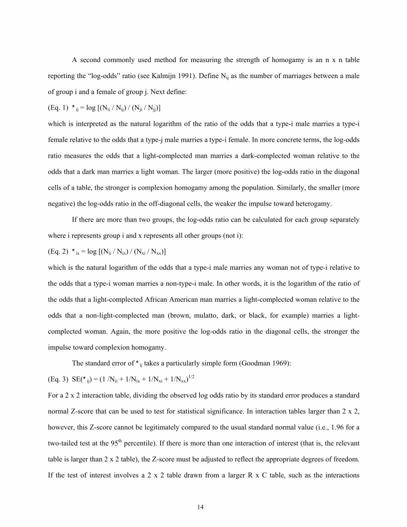
A second commonly used method for measuring the strength of homogamy is an n x n table

reporting the “log-odds” ratio (see Kalmijn 1991). Define Nij as the number of marriages between a male

of group i and a female of group j. Next define:

(Eq. 1) *ij = log [(Nii / Nij) / (Nji / Njj)]

which is interpreted as the natural logarithm of the ratio of the odds that a type-i male marries a type-i

female relative to the odds that a type-j male marries a type-i female. In more concrete terms, the log-odds

ratio measures the odds that a light-complected man marries a dark-complected woman relative to the

odds that a dark man marries a light woman. The larger (more positive) the log-odds ratio in the diagonal

cells of a table, the stronger is complexion homogamy among the population. Similarly, the smaller (more

negative) the log-odds ratio in the off-diagonal cells, the weaker the impulse toward heterogamy.

If there are more than two groups, the log-odds ratio can be calculated for each group separately

where i represents group i and x represents all other groups (not i):

(Eq. 2) *ix = log [(Nii / Nix) / (Nxi / Nxx)]

which is the natural logarithm of the odds that a type-i male marries any woman not of type-i relative to

the odds that a type-i woman marries a non-type-i male. In other words, it is the logarithm of the ratio of

the odds that a light-complected African American man marries a light-complected woman relative to the

odds that a non-light-complected man (brown, mulatto, dark, or black, for example) marries a light-

complected woman. Again, the more positive the log-odds ratio in the diagonal cells, the stronger the

impulse toward complexion homogamy.

The standard error of *ij takes a particularly simple form (Goodman 1969):

(Eq. 3) SE(*ij) = (1 /Nii + 1/Nix + 1/Nxi + 1/Nxx)1/2

For a 2 x 2 interaction table, dividing the observed log odds ratio by its standard error produces a standard

normal Z-score that can be used to test for statistical significance. In interaction tables larger than 2 x 2,

however, this Z-score cannot be legitimately compared to the usual standard normal value (i.e., 1.96 for a

two-tailed test at the 95th percentile). If there is more than one interaction of interest (that is, the relevant

table is larger than 2 x 2 table), the Z-score must be adjusted to reflect the appropriate degrees of freedom.

If the test of interest involves a 2 x 2 table drawn from a larger R x C table, such as the interactions

15

defined in Equation (2), then the appropriate Z-score test statistic is that corresponding to the (2.5/(R x

C))th percentile (assuming a two-tailed test at the underlying 95th percentile). Thus, if the test of interest

involves the 95th percentile of a 2 x 2 subtable drawn from a larger 5 x 5 table, the appropriate Z-score is

that corresponding to the 0.1th (2.5/25) percentile, which is 3.09, not the usual 1.96.

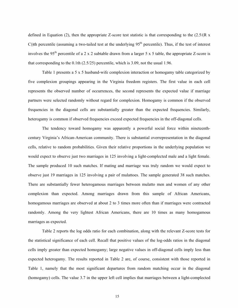
Table 1 presents a 5 x 5 husband-wife complexion interaction or homogamy table categorized by

five complexion groupings appearing in the Virginia freedom registers. The first value in each cell

represents the observed number of occurrences, the second represents the expected value if marriage

partners were selected randomly without regard for complexion. Homogamy is common if the observed

frequencies in the diagonal cells are substantially greater than the expected frequencies. Similarly,

heterogamy is common if observed frequencies exceed expected frequencies in the off-diagonal cells.

The tendency toward homogamy was apparently a powerful social force within nineteenth-

century Virginia’s African-American community. There is substantial overrepresentation in the diagonal

cells, relative to random probabilities. Given their relative proportions in the underlying population we

would expect to observe just two marriages in 125 involving a light-complected male and a light female.

The sample produced 10 such matches. If mating and marriage was truly random we would expect to

observe just 19 marriages in 125 involving a pair of mulattoes. The sample generated 38 such matches.

There are substantially fewer heterogamous marriages between mulatto men and women of any other

complexion than expected. Among marriages drawn from this sample of African Americans,

homogamous marriages are observed at about 2 to 3 times more often than if marriages were contracted

randomly. Among the very lightest African Americans, there are 10 times as many homogamous

marriages as expected.

Table 2 reports the log odds ratio for each combination, along with the relevant Z-score tests for

the statistical significance of each cell. Recall that positive values of the log-odds ratios in the diagonal

cells imply greater than expected homogamy; large negative values in off-diagonal cells imply less than

expected heterogamy. The results reported in Table 2 are, of course, consistent with those reported in

Table 1, namely that the most significant departures from random matching occur in the diagonal

(homogamy) cells. The value 3.7 in the upper left cell implies that marriages between a light-complected

16

male and a light complected female are 3.7 times more likely than a marriage between a light complected

female and a male of any other complexion. The result is both meaningful and statistically significant.

Values of the log-odds ratio reported in the other diagonal cells in Table 2, with the exception of brown-

brown cell, are also large and statistically significant. The only off-diagonal cell that approaches statistical

significance is the light male - mulatto female cell. The large and nearly significant negative value implies

that the lightest African Americans strictly observed complexion homogamy. Not only did they display a

strong impulse toward homogamy, but light-complected males displayed an equally strong impulse

against marrying women of darker complexions. This finding accords with the mathematical models of

homogamy developed by Burdett and Coles (1997) and Belding (2004) discussed in Section 2 above,

where a complexion-based separating equilibrium will naturally emerge in the marriage market as

individuals segregate themselves in complexion groups.

Because the federal censuses categorized African Americans as either black or mulatto, Tables 3

through 6 are 2 x 2 homogamy tables constructed from data reported in either the 1850 or the 1860

population manuscript censuses. Table 3 reports the results from a sample of 198 Maryland households in

1850. Random matching would imply just five mulatto-mulatto marriages, but we actually observe 24.

Because Table 3 is a simple 2 x 2 categorization, the log-odds ratios are symmetric (i.e., the diagonal cells

are the same, and the off-diagonal cells equal the negative log-odds ratio of the diagonals) and equal

5.14.19 This implies that the odds that mulatto man married a mulatto woman was 5 times the odds that a

black man married a mulatto woman. Tables 4 through 6 report comparable 2 x 2 tables for Baltimore,

Maryland; New Orleans, Louisiana; and Norfolk, Virginia in 1860. In all three instances, there are large

disparities between the observed and expected values in all cells, disparities consistent with complexion

homogamy. The number of mulatto-mulatto marriages in 1860 Baltimore, for example, is more than three

times as great as random mating would generate. The log-odds ratios for all three tables are also

consistent with complexion homogamy: 4.63 (Z-score = 18.52) for Baltimore; 4.11 (Z-score = 7.33) for

New Orleans; and 3.30 (Z-score = 4.23) for Norfolk.

19 The Z-score is 6.51, with a critical value of 1.96 for a two-tailed test at 99% significance.

17

Homogamy was a powerful impulse in the antebellum South. Light-complected blacks married

other light-complected blacks at rates far outside rates we would observe if mating was color blind.

Contemporary anecdotal evidence, as well as the findings of several historical studies, support these

empirical results. Light-complected blacks behaved as if the culture either strongly supported complexion

homogamy or punished complexion heterogamy. Moreover, the results are consistent with Olson’s belief

that groups capable of capturing rents will develop norms consistent with the continued collection of

those rents. In caste societies, intramarriage is a common and powerful norm. The next section

investigates the extent to which the norm toward complexion homogamy among light-complected blacks

protected the “preference” rents they received from whites and other blacks.

5. Economic Consequences of Complexion Homogamy

Data reported in the population manuscripts of the 1860 provide a rare opportunity to investigate the

economic consequences of colorism and complexion homogamy in the African-American community.

Olson (1982) and Smits (2004) argue that members of elite social and economic groups labor to insulate

themselves from lower status groups. Proscriptions against heterogamy maintain the boundaries between

elites and lower classes, which preserves assets, and status, intergenerationally. Although the census data

does not separately report the value of assets brought to a marriage by the husband and by the wife,

households made up of two light-complected spouses will have greater wealth than households with a

dark-complected spouse, all else constant, if Olson’s thesis holds. This section tests for complexion-based

differences in economic outcomes, including household wealth, controlling for a number of relevant

correlates. The results are consistent with Olson’s hypothesis in that households with two light-

complected spouses were wealthier than others.

Tables 7 and 8 motivate the argument that follows. Table 7 reports literacy rates by sex and

complexion for married spouses included in the sample. The most literate group was light complected

men married to light complected women (71 percent). The second most literate group (68 percent) was

light complected women married to light complected men. The least literate male-female combination

was the light male-dark female match, wherein only 51 percent of men and 32 percent of women were

18

literate. It appears that light males who selected dark females were less desirable males who attracted less

desirable females. Black men who attracted light women were no more literate, on average, than black

men who married black women. Educational homogamy is strong in modern societies (Smits 2004), and

was seemingly so among light-complected blacks in the antebellum South.

It seems likely that economic homogamy was also a powerful force in the early African-

American community. Table 8 reports average wealth cross-classified by sex and complexion. Light

male-light female marriages were the wealthiest by far, with about four times the wealth of black male-

light female and black male-black female marriages. Similarly, light-light marriages were more than

twice as wealthy as light-black households. Together, Tables 7 and 8 imply a powerful set of social

conventions that reinforced the norm of complexion homogamy. The remainder of this section uses

multiple regression techniques to control for factors that influenced household wealth, including

complexion homogamy.

5.1 The Determinants of Black Household Wealth

The empirical strategy of this section is to estimate household-level wealth regression equations

that include likely correlates between household wealth and household structure, including the

complexion composition of the marriage partners (i.e., whether the observed partners were light-light,

light-dark, dark-light, or dark-dark). The 1860 census provides a unique opportunity because it was the

first federal census to collect and report household-level information on a household’s real and personal

wealth; and was the second census to report the details of the age, sex, literacy, nativity, and occupation

of each household member. Additionally, and most importantly, it separated African-American

respondents into light- and dark-complected categories (mulatto and black). The estimated regressions

equations take the general form:

(Eq. 4) ln(Tj) = " + $1Xj + $2Yj + $3Zj + ((Light-Light)j + ,j

where the j’s index households so that ln(Tj)represent the natural logarithm of total household wealth; the

Xj’s capture the husband’s characteristics; the Yj’s capture the wife’s characteristics; the Zj’s capture

household characteristics; and the last term captures the complexion combinations of husbands and wives,

19

with the husband’s complexion listed first. The excluded category is any marriage involving a dark-

complected individual.20 The " represents the estimated constant parameter, the $k’s the relevant slope

coefficients, the ( the homogamy shift term, and ,j is the error term.

As with all empirical work using the federal manuscript census records there are several issues of

data quality that need to be addressed. First and most relevant, is that some census marshals were more

diligent in recording information than others. It was not uncommon for marshals to have returned

incomplete information on some households. Information on household structure is almost always

reported, along with sex and age of the household members. Male occupations were typically reported,

but blanks are not uncommon and are difficult to interpret. It is unclear whether the information was not

provided, if the person was unemployed, or if they were retired, though the last is discernible, to some

extent, by considering the respondent’s age. There were just 43 instances of nonreporting of occupation

for husbands in an original sample of 1,452 households. Those 43 cases were dropped from the sample

used in estimating the regression equations. Another 24 households were dropped because other pertinent

data was missing or clearly miscoded, leaving a final sample of 1,385 households.

The more perplexing problem in the use of data from the 1860 federal censuses is that

nonreporting of wealth data was not uncommon. Indeed, of the final household sample, marshals recorded

wealth data for just 967 (or 69.8 percent of households). Researchers have long debated the meaning of

the missing wealth data (Conley and Galenson 1994 provide a review). Some have interpreted it to imply

that a household had no tangible wealth, but it is hard to imagine 439 African-American households

owning absolutely nothing of discernible value. The personal property category in the 1860 federal census

was to include all household property (furniture, fixtures, kitchen utensils, and so forth) not otherwise

enumerated in the valuation of real property, and it is hard to imagine a viable household without at least

a few basic amenities. A second common interpretation is that households concealed or obscured wealth

20 Initial regressions were estimated with three marriage combinations (Light-Light, Light-Dark, and Dark-Light, with Dark-Dark as the excluded category). The estimated coefficients on Light-Dark, and Dark-Light were not statistically significant and were not significantly different from each other. Thus, the reported regressions include only a Light-Light category with the default excluded group including all marriages with at least one dark partner.

20

from authority figures who may have reported them to the tax collector. Again, this seems an

unreasonable interpretation, given that any household would have a difficult time concealing everything it

owned. A third, and more plausible, explanation is that marshals simply failed to report small wealth

holdings.

Rather than exclude households with no reported wealth, which eliminates a large proportion of

the sample, it is assumed that marshals had idiosyncratic lower-bound censoring thresholds. That is,

marshals regularly left the wealth cell blank for households failing to meet some minimum threshold. In a

study of 26 southern rural counties, Bodenhorn (2002) finds that most marshals tended to censor at values

less than $10, a few censored below $25, and a handful censored below $50. The strategy adopted here is

to impute a value for each nonreporting household equal to one-half the lowest value reported by any

marshal canvassing a city ward.21 For nonreporting households in Baltimore’s fifth ward, a wealth value

of $12.50 was imputed for each nonreporting household because the lowest reported value was $25,

which was approximately the median censoring threshold in these two city’s 31 wards. The lowest

censoring threshold was $3 in Baltimore’s seventeenth ward; the highest was $100 in three of Baltimore’s

20 wards and in 5 of New Orleans’ 11 wards.

The first column of Table 9 reports the means of the independent variables. The husband’s birth

cohort is included to capture age effects in wealth accumulation (the 1791-1800 cohort is the excluded

category).22 Older African American couples are likely to have accumulated more wealth than younger

couples. Not only did older couples have more time to save, but traditional histories hold that slaves freed

in the post-Revolutionary period were freed under particularly favorable circumstances (Berlin 1974).

The egalitarian impulse following the Revolution led many slaveholders to manumit slaves, providing

them with land, livestock, and cash or other assets to embark on a life under freedom. After the 1810s and

1820s, manumitting slaveholders were less generous.

21 Altonji, Doraszelski and Segal (2000) adopt a similar practice in a study involving modern data and determine that doing so introduces little bias while preserving sample size.

22 Alternative specifications including a quadratic in the husband’s age, with and without cohorts, generated few statistically significant coefficient estimates on the age variables and are not reported.

21

A second pair of independent variables are dummy variables taking a value of 1 if the husband

and/or wife migrated to Baltimore or New Orleans from another state or country. Migrants tend to be

more highly motivated or accomplished than people who stay behind. Because high productivity

individuals tend to self-select for migration, migrants and immigrants may have accumulated greater

wealth for a given set of characteristics. The regressions also include indicator variables capturing the

husband’s and/or wife’s illiteracy. Less educated people tend to earn lower incomes, which may lead to

lower savings rates and less accumulation of assets. The number of individuals residing in the household

is also included in the regrssions. Extended households may have had greater agglomerations of wealth

than nuclear families. An indicator variable for Baltimore was included to capture any city or regional

differences influencing the abilities of African-American households to accumulate wealth.

An important determinant of wealth is occupational status. High-status occupations tend to be

high-income occupations so that individuals with high status occupations are likely to accumulate more

wealth, everything else constant, than individuals laboring in low-status occupations. To capture

occupational status, the regressions include a socioeconomic index value (SEI) that corresponds to Otis

Dudley Duncan’s occupational socioeconomic index score. Rather than categorizing occupations into

broad categories (professional, skilled, unskilled, etc.) as is often done, this variable is capable of

capturing more subtle differences in occupation-related abilities to save and amass wealth. The

conventions followed here were the same as those followed in putting together the IPUMS data sets.

Using Duncan’s Index (see Reiss 1961) necessarily generates some anachronisms in job classifications.

Some occupations common in 1860 had disappeared by the 1950s when Duncan created his index. There

were few carriage drivers or draymen in the 1950s, for example, but there were taxi drivers (the 1950s

equivalent of the 1850s carriage driver) and truck drivers (the 1950s equivalent of the 1850s drayman)

and the modern codings were assigned to older occupations. When the modern equivalent of the

nineteenth-century occupation was less obvious, Duncan’s generic SEI score by job class (craftsman,

operative, or laborer) and industry (construction, metals, machinery, food and kindred products, leather

products, etc.) was assigned to the individual.

22

Finally, each regression includes an indicator variable (Light-Light) capturing the type of

marriage by complexion. The excluded category is a combination of Dark-Light, Light-Dark, and Dark-

Dark, or any household in which at least one of the partners was dark complected. Tables 7 and 8, and

some preliminary but unreported regressions suggest that households including a dark partner resembled

each other more closely than households made up of two light complected individuals. If Olson’s (1982)

contention that the purpose of homogamy among the elite is to preserve assets across generations holds,

the coefficient estimates on the Light-Light variable will be large, positive, and statistically significant.

Because light-complected individuals who marry dark may have violated a community norm, they may

have been punished or shunned. The group of light-complected blacks who married dark may also have

initially been outside the elite as their lower literacy rates attest (see Table 7), which implies that they

brought fewer assets to the marriages. But by marrying dark, these initially less wealthy light-complected

individuals effectively excluded themselves from later acceptance into the “mulatto elite.” Regardless of

whether light-complected blacks who married a dark partner were outsiders or were insiders shunned for

their choice, the homogamy norm was an effective exclusionary device.

The regressions were estimated using ordinary least squares (OLS), robust regression, and median

regression. Given the missing wealth data in the census, OLS regression is problematic because it may

return inconsistent estimates (Conley and Galenson 1994).23 Moreover, parameter estimates in

semilogarithmic specifications relying on the imputation of some value for missing or zero-value

observations are sensitive to different imputations. Despite potential estimation problems with OLS, it

remains a useful basis of comparison and the imputed values used here are reasonable and justified given

23 The equations were also estimated using maximum likelihood techniques for truncated and censored observations (using the truncreg and tobit commands in STATA). Truncated and censored data are generated by different sampling processes and should be handled differently. A sample is censored if no observations have been excluded, but some of the information contained in them is suppressed. This seems to explain the failure to record wealth information for some households. A truncated sample is one in which observations falling below some point are excluded. Given concerns with underenumeration in early censuses, it is possible that low-wealth households were more likely to be overlooked than medium- or high-wealth households. Regression techniques for truncated samples use only that part of the sample above the truncation point to generate coefficient estimates. Maximum likelihood estimates for truncated regressions were estimated with truncation points between $10 and $150. The regression coefficients (or marginal effects) for the tobit and truncated regressions were not substantially different in sign or magnitude from OLS estimates and are not reported.

23

the census marshals’ censoring practices. The values were not arbitrarily chosen (i.e., some very small

nonnegative value), as is often the case, to produce a mathematically defined value of the logarithm in

cases with missing or nonpositive values.

A second statistical concern is the presence of several large outliers. The smallest reported wealth

value was $3; the largest was $23,000, with a mean of $336 and standard error of $542. Rather than

discarding the outliers, the specifications were estimated by robust regression and median regression.

Robust regression uses an iterative weighting algorithm to reduce the influence of observations with large

residuals. Median (or least absolute deviation) regression is more apt to return unbiased parameter

estimates even when the basic assumptions underlying OLS break down. Median regression is also an

attractive method when the sample data contains outliers or is censored. Neither robust regression nor

median regression resolves all the estimation issues, but they provide reasonable estimates of the central

tendency of the data when the classical assumptions underlying OLS break down.

The second through fourth columns of Table 9 report parameter estimates generated by OLS,

robust regression, and median regression. The parameter estimates from the three techniques agree in

sign, significance, and general magnitude. Coefficients on the cohort indicator variables, for instance,

support the traditional interpretation that African-Americans who attained their freedom just after the

American Revolution were treated more generously than later freed slaves, though the estimates also

capture the positive age-wealth correlation found in most modern studies. It not possible to separate the

independent influences without knowing whether an individual was free-born or manumitted, which we

do not observe. According to the OLS estimate, the cohort of husbands born between 1831 and 1840 had

51 percent less wealth than the cohort born between 1791 and 1800 (e-0.718 = 0.49). Estimates from both

the robust and median regressions are consistent with, though somewhat smaller than, the OLS estimate.

Older cohorts had greater wealth than younger ones.

Literacy, as expected, had a meaningful influence on household wealth. Holding all else

constant, a household with an illiterate husband had just 72 percent of the wealth of one with a literate

male head. The impact of female illiteracy was modestly larger, which is surprising given that the census

24

marshals recorded occupations for only 220 of the 1,385 wives included in the sample.24 If the census

provides an accurate assessment of female labor force participation, female literacy was related to

household wealth in a more complex manner than through the wife’s ability to generate labor market

income and add to the savings of her family. If a woman’s literacy was positively associated with her

parent’s economic status and if married women were unlikely to be engaged in the labor market, the

correlation between household wealth and female literacy may reflect the wife’s ability to bring physical

and social capital, more so than human capital, to the marriage. It is little wonder that light-complected

men sought light-complected women who, on average, had more human capital (see Table 7).

Larger households are associated with greater wealth. And black households in Baltimore had

significantly less wealth than comparable households in New Orleans, a finding in accordance with

traditional interpretations of attitudes toward free blacks in the Upper and Lower South.

The findings most relevant to the issue of colorism and complexion homogamy are captured by

the coefficient estimates on the spouses’ complexion variables. Relative to either complexion

heterogamous or Dark-Dark homogamous households, homogamous Light-Light households had

significantly more wealth. The OLS estimates imply that light-complected homogamous marriages had

about 47 percent (e0.384 = 1.468) more wealth than homogamous dark marriages. The robust regression

estimates imply a modestly larger light complexion advantage, or a premium of about 50 percent. Median

regression estimates imply a smaller, but still substantial 39 percent advantage for the median household.

The light-light complexion homogamy advantage was statistically significant and economically

meaningful. Light-light homogamous marriages had one third to one half more household wealth than

dark-dark marriages.

Given the social norm toward complexion homogamy within the black community, particularly

the light-complected elite, it is possible that the Light-Light variable is endogenous. If it is, OLS estimates

are inconsistent and may not be close to the true value even in a large sample. Instrumental variable or

24 Wive’s occupational SEI’s were not included in the regressions because there were too few of them and because most were listed as “washer” or “laundress,” with a few listed as seamstresses or nurses, which generated little variation in the data to obtain a reliable coefficient estimate.

25

two-stage least squares (2SLS) can be used to correct for this inconsistency if a valid instrument can be

identified. The OLS regression was reestimated as a two-stage least squares regression using the age

difference between the marriage partners (male age minus female age) as the instrument.

The age difference between partners should a priori be a valid instrument because it should be

correlated with the potentially endogenous variable (Light-Light) and uncorrelated with the dependent

variables in the second stage (log wealth). Bogger (1997) and other historians recount often unsuccessful

attempts among elite free black men to find compatible partners their own age. If the impulse toward

complexion homogamy outweighed the impulse toward marrying another of similar age, we are more

likely to observe substantial age differentials among light-light homogamous pairings than among

heterogamous or dark-dark pairings. The first stage regression contains the full set of variables in addition

to the age difference of married couples. This regression is well specified. The F-statistic of the first-stage

regression is 32.04 and the chi-square statistic of the Hausman test is 0.01 with a p-value of 0.99. Thus,

the test fails to reject the null hypothesis that the OLS estimator is consistent.25 Thus, we are confident

that the coefficient on the OLS estimate captures the true, and powerful, effect of homogamous marriage

on wealth accumulation.

The findings reported in this section support Olson’s (1982) hypothesis that elite groups will

maintain their privileges intergenerationally by developing social conventions conducive to homogamy.

Although it is impossible to determine which spouse brought what to the marriages observed here, the

results suggest that light-light couples accumulated wealth than dark-dark or dark-light combinations. The

next section employs widely used Blinder-Oaxaca regression decomposition techniques to determine the

relative influence of systematic differences in household characteristics and differences in treatment on

household outcomes.26

25 The augmented regression test suggested by Davidson and McKinnon (1993) is consistent with the Hausman test. The p-value of the Light-Light coefficient in the augmented regression is 0.883, implying that the OLS estimator is consistent. With only one available instrument, the standard overidentification test is unavailable.

26 See Blinder (1973) and Oaxaca (1973) for the original derivations of the procedure. They are now widely used in the literature.

26

5.2 Did Those with Lighter Complexions Receive Better Treatment: Evidence from Regression

Decompositions

Wealth differences between any two groups may be due to differences in the average

characteristics of that group (characteristics effects), or to systematic variations in how a given

characteristic is rewarded in the marketplace and affects an individual’s ability to accumulate wealth

(treatment effects). The premise of this article is that colorism interacts with the complexion homogamy

norm such that light-light homogamous partners will receive preferential treatment, relative to

heterogamous pairings, for a given set of observable characteristics. This section explores the issue by

decomposing complexion wealth gaps using standard decomposition techniques.

The initial step in the decomposition methodology is to estimate separate regressions for relevant

subgroups. The sample is separated into four groups or subsamples. First, the groups are separated by

city, with separate regressions estimates by city. This decision is driven by both empirical and historical

considerations. The large and significantly negative parameter estimate on the Baltimore dummy variable

suggests different regional treatment, a common contention among historians of the antebellum black

experience. The city subsamples are then further separated by marriage type. Separate parameters are

estimated for light-light households in each city and compared to parameter estimates for households with

at least one black marriage partner (light-dark, dark-light, and dark-dark). These eight regressions are

reported in Table 10. Because there are some concerns that the socioeconomic index variable (SEI) may

be endogenous, regressions and decompositions are reported with and without the variable. The results do

not differ in any meaningful way.

Once these separate city-complexion subsample regressions are estimated, it is possible to predict

the wealth (ë) for a city-complexion type.27 For mulattos residing in Baltimore, for example, the

estimated mean household wealth of a light-light household is ëmm = µm $m, where µm represents the

vector of mean characteristics of mulattos and $m represents the vector of estimated regression

27 This discussion follows that found in Goldsmith, Hamilton, and Darity (2004).

27

coefficients for mulattoes appearing in the Baltimore subsample (city subscripts are suppressed). Next,

define ëmb = µm $b, where µm remains the vector of mean characteristics of light-light (mulatto)

households and $b is a vector of estimated regression coefficients for marriages involving a black spouse.

Other combinations are defined analogously, where the subscript on the ë refers to the mean group

characteristics and the superscript refers to the group parameter estimates.

Next, define the Treatment Advantage as: TA = (-1)[(ëmb - ëm

m) / ëmm]. The treatment advantage

measures the percentage wealth gain the preferred group receives as a result of the preferences shown it,

independent of any group characteristics that may provide its members with an ability to generate and

accumulate wealth. Because decompositions can be calculated from the viewpoint of either group, we can

also define the Treatment Disadvantage as TD = [(ëbm - ëb

b) / ëbb]. The treatment disadvantage measures

the percentage wealth shortfall realized by the discriminated-against group as a result of colorism,

independent of the group’s mean characteristics. By calculating treatment effects both ways, the analysis

generates a range of average estimated benefits associated with being a member of the preferred group.

In addition to treatment effects, the decomposition procedure makes it possible to produce

estimates of the percentage of the complexion-based wealth gap explained by differences in group

characteristics. The analog of the treatment advantage is the Characteristic Advantage, which is

calculated as: CA = (-1)[(ëbm - ëm

m) / ëmm]. The characteristic advantage takes the preferred group as the

reference group and estimates the percentage of the wealth gap attributable to differences in household

characteristics that influence the generation and accumulation of wealth. The Characteristic

Disadvantage is calculated as: CD = [(ëmb - ëb

b) / ëbb], which uses households with a black spouse as the

reference group and provides an estimate of the wealth shortfall of households with a black spouse due to

differences in productive characteristics.

Table 11 provides estimates of Treatment Effects and Characteristic Effects for Baltimore and

New Orleans based on the OLS regressions reported in Table 10. The second column of Table 11 reveals

that the estimated wealth of households with a black spouse ranged between 88.8 and 91.6 percent of the

wealth of light-light households. Subsequent columns report estimates of the Treatment and Characteristic

Effects. Treatment advantages experienced by light-light households ranged between 8.4 and 9.3 percent

28

of average estimated wealth in Baltimore. In New Orleans treatment advantages experienced by

households with two light-complected households varied from 7.3 to 7.4 percent of estimated wealth.

Estimates of the treatment disadvantages experienced by Baltimore households with at least one black

spouse parallel the estimated advantages when using light-light households as the reference group. They

range between 7.9 and 9.4 percent of average estimated wealth.

Differences in wealth-producing characteristics account for a much smaller fraction of the

complexion-based wealth gaps than the treatment effects. In the Baltimore subsample, the characteristic

advantage experienced by mulatto households was 2.7 to 4.4 percent; it was 1.6 for both models in New

Orleans. If we use households with at least one black spouse as the reference group, the characteristic

disadvantage ranges between 2.1 and 3.3 percent in Baltimore and 1.2 and 1.3 percent in New Orleans.

Differences in wealth-producing characteristics account for about one-fourth to about one-half as much of

the complexion wealth gap as differences in treatment. Thus, while differences in household

characteristics account for some of the differences observed between dark and light households, treatment

effects account for a much larger share of the wealth gap. The results are consistent with the colorism

hypothesis.

6. Concluding Remarks

This paper demonstrates that one implication of intraracial black colorism was complexion homogamy.

Light-complected blacks married light-complected blacks, darks married darks, and there was less

complexion mixing than would be expected if love was truly color blind. Homogamy was the norm and

there were apparently strong social conventions within the black community supporting the practice.

Some scholars have noted its persistence to modern times (Udry, Bauman and Chase 1971; Graham

1999). The black elite in major U.S. cities remains overwhelmingly light complected and its members

encourage their children to mingle with others of like complexion.

A second finding of the paper is that light-light complexion homogamous households have more

wealth than complexion heterogamous or dark-dark homogamous households. An implication of this

finding is that complexion homogamy generates an intergenerational persistence of status, education, and

29

wealth. In this regard complexion homogamy was not (and is) not an innocuous tradition. It had (and has)

significant social and economic ramifications. Homogamous marriage practices have the benefit of

preserving assets and status among the existing elite, but it may deny access to deserving individuals

outside the elite. Graham (1999), for example, documents instances in which the light complected elite

still use exclusive clubs and organizations to deny access to important social and economic networks

(social capital) to the emerging black middle class. Gatewood (2000) dated to practice to Reconstruction

and Williamson (1980) reports some evidence of it in antebellum Charleston, South Carolina. This paper

pushes the twin traditions of colorism and complexion homogamy back to the Early National Period and

broadens its geographic scope. Light complected blacks have seemingly maintained their elite position in

the United States through homogamy for more than two centuries. On one hand, social capital like that

developed through clubs and organizations can be an effective mechanism for advancement, which

appears to have been an important element in the success achieved by light-complected men and women

in the antebellum South. On the other, the exclusivity of clubs and organizations can have negative

consequences for outsiders (Fukuyama 1999). Because they are denied access to valuable social and

economic networks, outsiders find advancement difficult because there is a connection between the

accumulation of social capital and access to economic resources. Future research should more fully

investigate the extent to which the black elite’s networks exclude nonelite blacks and the consequences of

that exclusion for black advancement.

Data Appendix

Virginia Freedom Registers

Alleghany County: Register of Free Negroes and Mulattoes in Alleghany County, 1855-1856. Microfilm

at Library of Virginia (hereafter LOV).

Arlington County: Register of Free Negroes, 1797-1861. LOV.

Bedford County: Register of Free Negroes, 1803-1820. LOV.

Augusta County: Katherine Bushman (ed.). 1989. The Registers of Free Blacks, 1810-1864: Augusta

County, Virginia and Staunton, Virginia. Verona: Va.: Mid-Valley Press, Inc.

30

Botetourt County: Dorothy A. Boyd-Rush (ed.). 1993. Free Negroes Registered in the Clerk’s Office,

Botetourt County, Virginia, 1802-1836. Athens, Ga.

Brunswick County: Frances Holloway Wynne. 1983. Register of Free Negroes and also of Dower Slaves:

Brunswick County, Virginia, 1803-1860. Fairfax, Va.

Campbell County: Register of Free Negroes, 1801-1850. LOV.

Charles City County: Register of Free Negroes, 1839-1864. LOV.

Chesterfield County: Register of Free Negroes, 1804-1854. LOV.

Cumberland County: Register of Free Negroes, 1821-1863. LOV.

Essex County: Register of Free Negroes, 1843-1861. LOV.

Fairfax County: Donald Sweig. 1977. Registrations of Free Negroes Commencing September Court 1822,

Book No. 2 and Register of Free Blacks 1835 Book 3. Fairfax, Va.: Office of Comprehensive

Planning.

Fauquier County: Karen King Ibrahim, Karen Hughes White and Courtney Gaskins. 1993. Fauquier

County, Virginia Register of Free Negroes, 1817-1865. Afro-American Historical Association of

Fauquier County.

Fluvanna County: Register of Free Negroes, 1851-1862. LOV.

Lancaster County: Register of Free Negroes, 1803-1860. LOV.

Middlesex County: Register of Free Negroes, 1800-1860. LOV.

Montgomery County: Richard B. Dickenson. 1981. Entitled! Free Papers in Appalachia Concerning

Antebellum Freeborn Negroes and Emancipated Blacks of Montgomery County, Virginia.

Washington, DC: National Genealogical Society.

Northampton County: Frances Bibbins Latimer. 1992. The Register of Free Negroes: Northampton

County Virgnia, 1853 to 1861. Bowie, Md.: Heritage Books, Inc.

Orange County: Free Negro Papers, 1837-1850. LOV.

Rockingham County: Dorothy A. Boyd-Rush (ed.). 1992. Register of Free Blacks, Rockingham County,

Virginia, 1807-1859. Bowie, Md.: Heritage Books, Inc.

Westmoreland County: Register of Free Negroes, etc., 1828-1849. LOV.

31

References

A Colored American. “Prejudice among Ourselves.” The Colored American (19 August 1837).

Adams, John W. and Alice Bee Kasakoff. 1991. “Estimates of Census Underenumeration Based on

Genealogies.” Social Science History 15:x (month), 527-543.

Altonji, Joseph G., Ulrich Doraszekski, and Lewis Segal. 2000. “Black/White Differences in Wealth.”

Federal Reserve Bank of Chicago Economic Perspectives 24:1, 38-50.

Anonymous. “What Becomes of the Free Colored People?” The National Era (5 October 1854).

Becker, Gary. 1971. The Economics of Discrimination. Second edition. Chicago and London: University

of Chicago Press.

Becker, Gary. 1981. A Treatise on the Family. Cambridge, MA: Harvard University Press.

Belding, Theodore C. 2004. “Nobility and Stupidity: Modeling the Evolution of Class Endogamy.”

Technical Report CSCS-2004-001, University of Michigan Center for the Study of Complex

Systems. Available at http://arXiv.org/abs/nlin/0405048.

Berlin, Ira. 1974. Slaves without Masters: The Free Negro in the Antebellum South. New York: The New

Press.

Bernheim, B. Douglas. 1994. “A Theory of Conformity.” Journal of Political Economy 102:5 (October),

841-77.

Blinder, Alan S. 1973. “Wage Discrimination: Reduced Form and Structural Estimates.” Journal of

Human Resources 8:x (month), 436-55.

Blocker, Jack S. 1996. “Bias in Wealth and Income Records: An Ohio Case Study.” Historical Methods

29:x (month), 25-36.

Bodenhorn, Howard. 1999. “A Troublesome Caste: Height and Nutrition of Antebellum Virginia’s Rural

Free Blacks.” Journal of Economic History 59:4 (December), 972-96.

Bodenhorn, Howard. 2002. “The Mulatto Advantage: The Biological Consequences of Complexion

among Free Blacks in Antebellum Virginia.” Journal of Interdisciplinary History 33:1 (Summer),

21-46.

32

Bogger, Tommy L. Free Blacks in Norfolk, Virginia, 1790-1860: The Darker Side of Freedom.

Charlottesville and London: University Press of Virginia, 1997.

Borjas, George. 1994. “Economics of Immigration.” Journal of Economic Literature 32:4 (December),

1667-1717.

Borjas, George. 2000. “Ethnic Enclaves and Assimilation.” Swedish Economic Policy Review 7:2 (Fall),

89-122.

Burdett, Ken and Melvyn G. Coles. 1997. “Marriage and Class.” Quarterly Journal of Economics 112:1

(February), 141-168.

Conley, Timothy G. and David W. Galenson. 1994. “Quantile Regression Analysis of Censored Wealth

Data.” Historical Methods 27: (month), 149-165.

Davidson, R. and J. G. MacKinnon. 1993. Estimation and Inference in Econometrics. New York: Oxford

University Press.

Davis, Kingsley. 1941. “Intermarriage in Caste Societies.” American Anthropologist (New Series) 43:3

(July), 376-395.

Davis, F. James. 1991. Who is Black? One Nation’s Definition. University Park, Pa.: The Pennsylvania

State University Press.

Dribe, Martin and Christer Lundh. 2004. “Finding the Right Partner: Rural Homogamy in Nineteenth-

Century Sweden.” Working paper, Lund University.

Dronkers, Japp and Huibert Schijf. 2003. “Marriages between Nobility and High Bourgeoisie as a Way to

Maintain Their Elite Positions in Modern Dutch Society.” Paper presented at European

Sociological Association Conference (September).

Ehrenberg, Ronald G. and Robert S. Smith. 2000. Modern Labor Economics: Theory and Policy. 7th

edition. Reading, Mass.: Addison-Wesley.

Frazier, E. Franklin. 1957. Black Bourgeoisie. New York: The Free Press.

Fukuyama, Francis. 1999. “Social Capital and Civil Society.” Paper presented at IMF Conference on

Second Generation Reforms. (October). Available at IMF web site.

33

Gatewood, Willard B. 2000. Aristocrats of Color: The Black Elite, 1880-1920. Fayetteville, Ark.:

University of Arkansas Press.

Goldsmith, Arthur H., Darrick Hamilton, and William Darity, Jr. 2004. “From Dark to Light: Skin Color and

Wages among African-Americans.” Unpublished working paper (August).

Goodman, Leo A. 1969. “How to Ransack Social Mobility Tables and Other Kinds of Cross-

Classification Tables.” American Journal of Sociology 75:1 (July), 1-40.

Graham, Lawrence Otis. 1999. Our Kind of People: Inside America’s Black Upper Class. New York:

Harper Collins Publishers.

Hill, Mark E. 2001. “Color Differences in the Socioeconomic Status of African American Men: Results of

a Longitudinal Study.” Social Forces 78:4 (June), 1437-1460.

Horton, James Oliver. 1993. Free People of Color: Inside the African American Community. Washington,

D.C. and London: Smithsonian Institution Press.

Hughes, Michael and Bradley R. Hertel. 1990. “The Significance of Color Remains: A Study of Life

Chances, Mate Selection, and Ethnic Consciousness among Black Americans.” Social Forces

68:4 (June), 1105-20.

Johnson, Whittington B. 1996. Black Savannah, 1788-1864. Fayetteville, Ark.: University of Arkansas

Press.

Kalmijn, Matthijs. 1991. “Shifting Boundaries: Trends in Religious and Educational Homogamy.”

American Sociological Review 56:6 (December), 786-800.

Kalmijn. Matthijs. 1994. “Assortative Mating by Cultural and Economic Occupational Status.” American

Journal of Sociology 100:2 (September), 422-52.

Kalmijn, Matthijs. 1998. “Intermarriage and Homogamy: Causes, Patterns, Trends.” Annual Review of

Sociology 24, 395-421.

Kandori, Michihiro. 1992. “Social Norms and Community Enforcement.” Review of Economic Studies

59: 1 (January), 63-80.

Keith, Verna M. and Cedric Herring. 1991. “Skin Tone and Stratification in the Black Community.”

American Journal of Sociology 97:3 (November), 760-778.

34

Komlos, John. 1992. “Toward an Anthropometic History of African-Americans: The Case of the Free

Blacks in Antebellum Maryland.” In Strategic Factors in Nineteenth Century American

Economic History: A Volume to Honor Robert W. Fogel, 297-329. Edited by Claudia Goldin and

Hugh Rockoff. Chicago and London: University of Chicago Press.

Litwack, Leon F. 1961. North of Slavery: The Negro in the Free States, 1790-1860. Chicago: University

of Chicago Press.

Manski, Charles F. 2000. “Economic Analysis of Social Interactions.” Journal of Economic Perspectives

14:3 (Summer), 115-36.

Margo, Robert A. Race and Schooling in the South, 1880-1950. Chicago and London: University of

Chicago Press, 1990.

Oaxaca, Ronald. 1973. “Male-Female Earning Differentials in Urban Labor Markets.” International

Economic Review 14:x (month), 693-709.

Olson, Mancur. 1965. The Logic of Collective Action: Public Goods and the Theory of Groups.

Cambridge, Mass.: Harvard University Press.

Olson, Mancur. 1982. The Rise and Decline of Nations: Economic Growth, Stagflation, and Social

Rigidities. New Haven and London: Yale University Press.

Reiss, Albert J. 1961. Occupations and Social Status. New York: The Free Press.

Reuter, Edward B. 1917. “The Superiority of the Mulatto.” American Journal of Sociology 23:1 (July),

83-106.

Smits, Jeroen. 2004. “Social Closure among the Higher Educated: Trends in Educational Homogamy in

55 Countries.” Unpublished working paper available at http://home.planet.nl/~smits.jeroen.

Toplin, Robert B. 1979. “Between Black and White: Attitudes toward Southern Mulattoes, 1830-1861.”

Journal of Southern History 45:2 (May), 185-200.

Udry, J, Richard, Karl E. Bauman, and Charles Chase. 1971. “Skin Color, Status, and Mate Selection.”

American Journal of Sociology 76: 4 (January), 722-733.

Williamson, Joel. 1980. New People: Miscegenation and Mulattoes in the United States. New York: The

Free Press.

35

Young, H. Peyton. 1996. “The Economics of Convention.” Journal of Economic Perspectives 10:2

(Spring), 105-22.

36

Table 1: Homogamy within Nineteenth-Century Virginia’s African-American Community Observed / Expected Frequencies by Complexion Combinations Husbands

Wives Light Mulatto Brown Dark Black

Light 10 / 2 0 / 4 1 / 1 1 / 1 0 / 3

Mulatto 2 / 10 38 / 19 4 / 6 3 / 6 7 / 13

Brown 7 / 3 2 / 7 6 / 2 0 / 2 4 / 5

Dark 2 / 3 0 / 6 1 / 2 11 / 2 2 / 4

Black 1 / 4 4 / 8 2 / 2 0 / 3 17 / 6

Notes: Random marriage probabilities calculated assuming no colorism as follows: Assume 125 males, of which 22 are light, 44 are mulatto, 14 are brown, 15 are dark, and 30 are black (column totals), and 125 females in proportion to their row totals. Label each male from 1 to 125 and each female from 1 to 125. The size of the event of interest is the number of all possible male-female pairs, which in this case is 15,625 (125 time 125) because there are 125 choices for males and 125 choices for females assuming any male-female pair is possible. The probability of a light male-light female marriage is 0.017 (22 males x 12 females all divided by 15,625). The expected number Sources: Virginia freedom registers. See data appendix.

37

Table 2: Homogamy within Nineteenth-Century Virginia’s African-American Community Log Odds Ratios and Z-statistics (in parentheses) by Complexion Combinations Husbands

Wives Light Mulatto Brown Dark Black

Light 3.7‡ (4.44)

-0.3 (-0.28)

-0.5 (-0.46)

Mulatto -2.3 (-3.00)

3.2‡ (6.22)

-0.7 (-1.13)

-1.2 (-1.79)

-1.2 (-2.51)

Brown 1.3 (2.36)

-1.7 (-2.20)

1.8 (2.92)

-0.1 (-0.16)

Dark -0.5 (-0.63)

-1.3 (-1.21)

4.0‡ (5.39)

-1.7 (-2.14)

Black -1.8 (-1.71)

-1.5 (-2.55)

-0.4 (-0.5)

2.8‡ (17.35)

Notes: ‡ implies statistical significance at 95th percentile. See text following Eqs. (1) and (2) for discussion of the calculation of Z-statistics for interaction tables of size (R x C). Critical Z-value is 3.09. Sources: Virginia freedom registers. See data appendix. Table 3: Homogamy among Black Residents of Maryland in 1850 Observed / Expected Frequencies by Complexion Combinations Mulatto Male Black Male

Mulatto Female 24 / 5 2 / 21

Black Female 14 / 33 158 / 139

Notes: Expected frequencies reflect underlying probabilities if marriage partners were selected randomly without regard for complexion. Calculated from complexion percentages by gender in sample. Sources: Population census manuscripts for Maryland (1850).

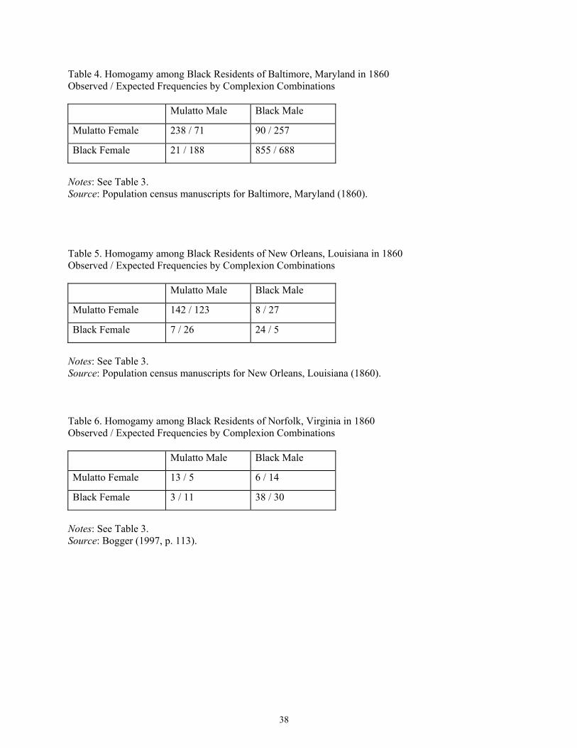
38

Table 4. Homogamy among Black Residents of Baltimore, Maryland in 1860 Observed / Expected Frequencies by Complexion Combinations Mulatto Male Black Male

Mulatto Female 238 / 71 90 / 257

Black Female 21 / 188 855 / 688

Notes: See Table 3. Source: Population census manuscripts for Baltimore, Maryland (1860). Table 5. Homogamy among Black Residents of New Orleans, Louisiana in 1860 Observed / Expected Frequencies by Complexion Combinations Mulatto Male Black Male

Mulatto Female 142 / 123 8 / 27

Black Female 7 / 26 24 / 5

Notes: See Table 3. Source: Population census manuscripts for New Orleans, Louisiana (1860). Table 6. Homogamy among Black Residents of Norfolk, Virginia in 1860 Observed / Expected Frequencies by Complexion Combinations Mulatto Male Black Male

Mulatto Female 13 / 5 6 / 14

Black Female 3 / 11 38 / 30

Notes: See Table 3. Source: Bogger (1997, p. 113).

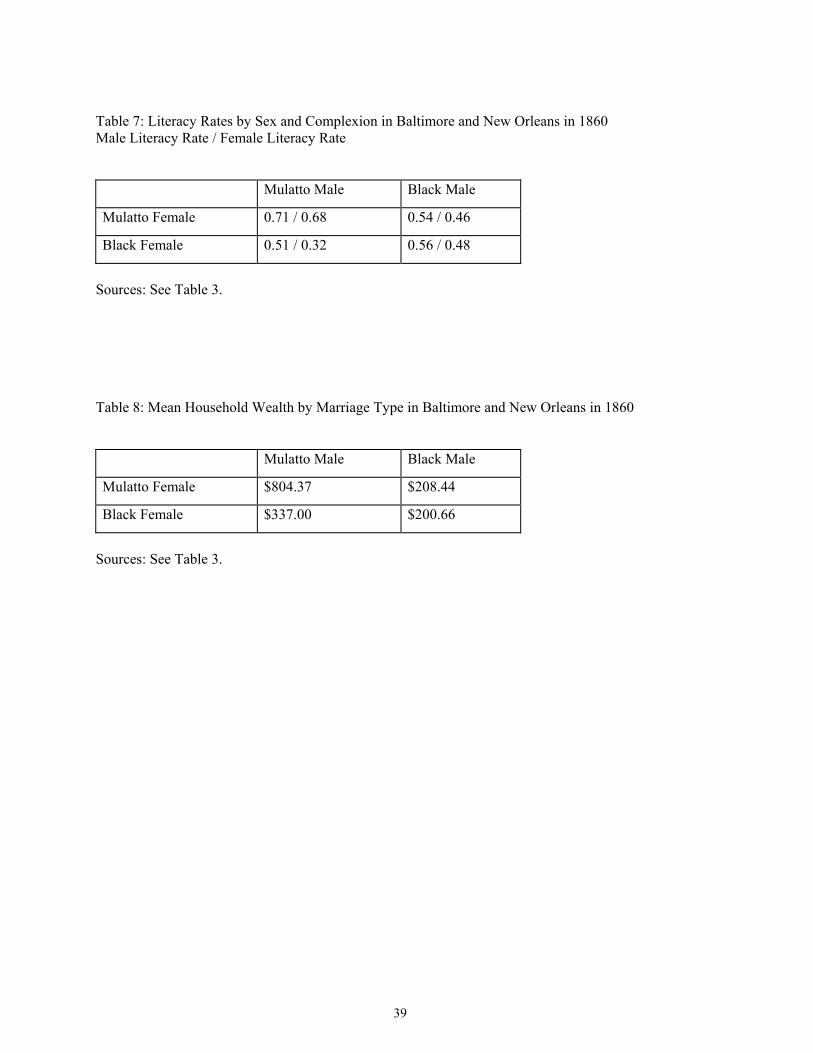
39

Table 7: Literacy Rates by Sex and Complexion in Baltimore and New Orleans in 1860 Male Literacy Rate / Female Literacy Rate Mulatto Male Black Male

Mulatto Female 0.71 / 0.68 0.54 / 0.46

Black Female 0.51 / 0.32 0.56 / 0.48

Sources: See Table 3. Table 8: Mean Household Wealth by Marriage Type in Baltimore and New Orleans in 1860 Mulatto Male Black Male

Mulatto Female $804.37 $208.44

Black Female $337.00 $200.66

Sources: See Table 3.

40

Table 9: Determinants of Household Wealth among African Americans in 1860 Baltimore and New Orleans (Dependent variable = ln(household wealth)) OLSa Robust Median Regression Regression Variable Mean Coefficient Coefficient Coefficient (S.E.) (S.E.) (S.E.) (S.E.) Cohort 1801-10 0.136 -0.247 -0.263 -0.283 (0.343) (0.201) (0.216) (0.213) Cohort 1811-20 0.374 -0.542‡ -0.509‡ -0.486† (0.484) (0.197) (0.201) (0.198) Cohort 1821-30 0.316 -0.751‡ -0.727‡ -0.621‡ (0.465) (0.179) (0.203) (0.200) Cohort 1831-40 0.136 -0.773‡ -0.706‡ -0.609‡ (0.343) (0.226) (0.217) (0.215) Male Mover 0.072 0.252 0.241 0.084 (0.259) (0.160) (0.158) (0.157) Female Mover 0.057 -0.091 -0.053 0.091 (0.232) (0.191) (0.176) (0.174) Male Illiterate 0.393 -0.313† -0.276‡ -0.162* (0.489) (0.151) (0.089) (0.087) Female Illiterate 0.468 -0.366† -0.421‡ -0.243‡ (0.499) (0.175) (0.088) (0.087) Household Size 6.170 0.044† 0.044‡ 0.040† (2.175) (0.019) (0.017) (0.017) ln (SEI) 2.477 0.404‡ 0.445‡ 0.409‡ (0.568) (0.127) (0.066) (0.065) Baltimore 0.869 -1.098‡ -1.061‡ -1.351‡ (0.337) (0.251) (0.124) (0.123) Light-Light 0.274 0.384‡ 0.406‡ 0.329‡ (0.446) (0.084) (0.093) (0.091) Constant 4.787‡ 4.632‡ 4.778‡ (0.507) (0.311) (0.308) No. Obs. 1,385 1,385 1,385 1,385 F-stat 36.27‡ 34.41‡ Adj-R2 0.22 0.09 Notes: a standard errors adjusted for clustering by census ward. ‡ implies statistical significance at 1% level; † at 5%; and * at 10%.

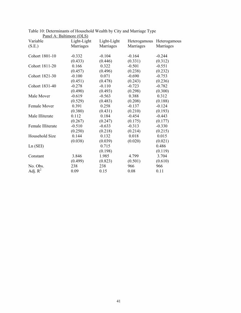
41

Table 10: Determinants of Household Wealth by City and Marriage Type Panel A: Baltimore (OLS) Variable Light-Light Light-Light Heterogamous Heterogamous (S.E.) Marriages Marriages Marriages Marriages Cohort 1801-10 -0.332 -0.104 -0.164 -0.244 (0.433) (0.446) (0.331) (0.312) Cohort 1811-20 0.166 0.322 -0.501 -0.551 (0.457) (0.496) (0.238) (0.232) Cohort 1821-30 -0.100 0.071 -0.690 -0.753 (0.451) (0.478) (0.243) (0.236) Cohort 1831-40 -0.278 -0.110 -0.723 -0.782 (0.490) (0.493) (0.298) (0.300) Male Mover -0.619 -0.563 0.388 0.312 (0.529) (0.483) (0.208) (0.188) Female Mover 0.391 0.258 -0.137 -0.124 (0.380) (0.431) (0.210) (0.193) Male Illiterate 0.112 0.184 -0.454 -0.443 (0.267) (0.247) (0.175) (0.177) Female Illiterate -0.510 -0.633 -0.313 -0.330 (0.250) (0.218) (0.214) (0.215) Household Size 0.144 0.132 0.018 0.015 (0.038) (0.039) (0.020) (0.021) Ln (SEI) 0.715 0.486 (0.198) (0.119) Constant 3.846 1.985 4.799 3.704 (0.499) (0.823) (0.501) (0.610) No. Obs. 238 238 966 966 Adj. R2 0.09 0.15 0.08 0.11

42

Table 10 continued: Panel B: New Orleans (OLS estimates) Light-Light Light-Light Heterogamous Heterogamous Marriages Marriages Marriages Marriages Cohort 1801-10 -0.024 0.043 -1.022 -1.020 (0.148) (0.522) (0.825) (0.838) Cohort 1811-20 -1.098 -1.042 -2.980 -2.978 (0.423) (0.474) (0.194) (0.197) Cohort 1821-30 -1.376 -1.312 -2.754 -2.736 (0.287) (0.596) (0.211) (0.289) Cohort 1831-40 -0.987 -0.926 -3.726 -3.698 (0.435) (0.597) (0.465) (0.602) Male Mover 0.607 0.607 0.074 0.077 (0.581) (0.584) (0.876) (0.885) Female Mover -0.552 -0.568 0.711 0.697 (0.580) (0.534) (0.865) (0.822) Male Illiterate -0.328 -0.329 0.119 0.124 (0.219) (0.229) (0.352) (0.327) Female Illiterate 0.113 0.117 0.114 0.097 (0.318) (0.337) (0.429) (0.402) Household Size 0.154 0.156 0.059 0.055 (0.021) (0.021) (0.076) (0.059) Ln (SEI) -0.044 0.038 (0.323) (0.291) Constant 5.840 5.891 7.566 7.486 (0.350) (0.504) (0.680) (1.185) No Obs. 142 142 39 39 Adj R2 0.14 0.14 0.37 0.37

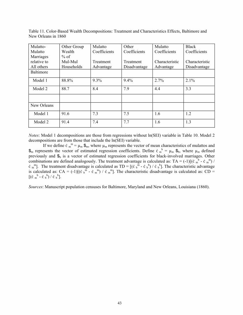
43

Table 11. Color-Based Wealth Decompositions: Treatment and Characteristics Effects, Baltimore and New Orleans in 1860 Mulatto-Mulatto Marriages relative to All others

Other Group Wealth % of Mul-Mul Households

Mulatto Coefficients Treatment Advantage

Other Coefficients Treatment Disadvantage

Mulatto Coefficients Characteristic Advantage

Black Coefficients Characteristic Disadvantage

Baltimore

Model 1 88.8% 9.3% 9.4% 2.7% 2.1%

Model 2 88.7 8.4 7.9 4.4 3.3

New Orleans

Model 1 91.6 7.3 7.5 1.6 1.2

Model 2 91.4 7.4 7.7 1.6 1.3

Notes: Model 1 decompositions are those from regressions without ln(SEI) variable in Table 10. Model 2 decompositions are from those that include the ln(SEI) variable. If we define ëm

m = µm $m, where µm represents the vector of mean characteristics of mulattos and $m represents the vector of estimated regression coefficients. Define ëm

b = µm $b, where µm defined previously and $b is a vector of estimated regression coefficients for black-involved marriages. Other combinations are defined analogously. The treatment advantage is calculated as: TA = (-1)[(ëm

b - ëmm) /

ëmm]. The treatment disadvantage is calculated as TD = [(ëb

m - ëbb) / ëb

b]. The characteristic advantage is calculated as: CA = (-1)[(ëb

m - ëmm) / ëm

m]. The characteristic disadvantage is calculated as: CD = [(ëm

b - ëbb) / ëb

b]. Sources: Manuscript population censuses for Baltimore, Maryland and New Orleans, Louisiana (1860).