the eco-indicator 95€¦ · the noh does not guarantee the correctness and/or completeness of...
TRANSCRIPT

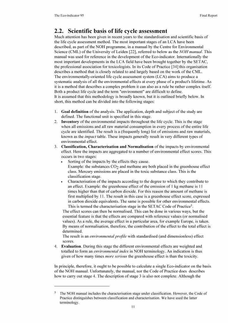
The Eco-indicator 95Weighting method for environmental effects that damage ecosystems
or human health on a European scale.
Contains 100 indicators for important materials and processes.
Final Report
Effect
CO
SO
Pb
Greenhouse effect
Ozone layer depl.
Eutrophication
Winter smog
CFC
Health
Fatalities
Ecosystem
Impact
Heavy metals
Pesticides
Carcinogenics
Summer smog
impairment
impairment
Acidification
Valuation
Subjective
assessment
Damage
damage
PAH
DDT
VOC
NO
Dust
Cd
P
Eco-indicator
value
Result
2
2
x
On the initiative of:
• Nederlandse Philips bedrijven BV
• Océ Nederland BV
• Netherlands Car BV
• Machinefabriek Fred A. Schuurink BV
With the cooperation of:
• University of Leiden (CML)
• University of Amsterdam (IDES, Environmental Research)
• Technical University of Delft (Industrial Design Engineering)
• Centre for Energy Conservation and Environmental Technology Delft
• TNO Product Centre
• Ministry of Housing, Spatial Planning and the Environment (VROM)
Author:
Mark Goedkoop of PRé Consultants

The Eco-indicator 95 Final Report
ii
Colophon
Contract number: 353194 / 1711
The Eco-indicator 95, Final Report
This project was carried out and financed under the auspices of the National Reuse of Waste
Research Programme (NOH). Management and co-ordination of the NOH programme are
the responsibility of:
Novem Netherlands agency for energy and the environment
St. Jacobssstraat 61 P. O. Box 8242
3503 RE Utrecht the Netherlands
Telephone: +31 (0)30-363444
Project managers: Ms. J. Hoekstra, J. v.d. Velde
RIVM National Institute of Public Health and Environmental Protection
Antonie van Leeuwenhoeklaan 9 P. O. Box 1
3720 BA Bilthoven the Netherlands
Telephone: +31 (0)30-749111
Project manager: G. L. Duvoort
The NOH does not guarantee the correctness and/or completeness of data, designs,
constructions, products or production processes included or described in this report or their
suitability for any specific application.
The project was carried out by:
• PRé Consultants
• DUIJF Consultancy BV1
In addition to this final report a manual for designers and an appendix are available. The
manual describes the practical application of the Eco-indicators. The appendix, which is
only available in Dutch, describes the full contribution of the cooperating institutes and the
full impact tables. Additional copies of this report, the manual for designers and the
appendix are available from:
PRé Consultants
Bergstraat 6 3811 NH Amersfoort the Netherlands
Telephone: +31 (0)33 611046 (as from October 1st +31 (0)33 4611046)
Telefax: +31 (0)33 652853 (as from October 1st +31 (0)33 4652853)
e-mail: [email protected]
NOH report 9523 The Eco-indicator 95, Final Report Dfl. 45.00
NOH report 9524 The Eco-indicator 95, Manual for Designers Dfl. 25.00
NOH report 9514 A De Eco-indicator 95, bijlagerapport (only in Dutch) Dfl. 55.00
The reports 9523 and 9524 are also available in Dutch at the same cost. For shipment abroad
Fl 20,- postage and packaging costs will be charged extra. The NOH has made it possible to
give a discount off the price of reports used for educational purposes.
ISBN 90-72130-80-4
1 At 25.1.1995 Duijf Consultancy BV went out of business.

The Eco-indicator 95 Final Report
iii
ContentsPreface 1
Summary 3
1. Introduction 5
1.1. Life cycle assessment 5
1.2. Aim of the project 5
1.3. Environmentally-aware design 5
1.4. Project working method 6
1.5. Project team and supervisory group 7
1.6. Government policy during this project 8
2. Life cycle assessment method 10
2.1. Qualitative methods 10
2.1.1. Red flag methods 10
2.1.2. MET matrix 10
2.2. Scientific basis of life cycle assessment 11
2.3. Weighting principles 12
2.3.1. EPS system 12
2.3.2. Prevention costs of emissions 14
2.3.3. Energy consumption needed to prevent emissions 14
2.3.4. Energy consumption as a measure of total environmental pollution 15
2.3.5. Evaluation by experts (panel method) 16
2.3.6. Ecopoints 16
2.4. Requirements for an Eco-indicator weighting method 17
2.4.1. Goal 17
2.4.2. Requirements and wishes 17
2.4.3. Selection of the weighting principle 18
3. Eco-indicator weighting method 19
3.1. Weighting according to Distance-to-Target 19
3.1.1. Policy or science 20
3.1.1.1. Politically determined target values 21
3.1.1.2. Scientifically determined target values 21
3.1.2. Definition of the term "environment" 21
3.1.2.1. Physical ecosystem degradation 22
3.1.2.2. Raw materials depletion 22
3.1.2.3. Space requirement for final waste 23
3.1.2.4. Toxicity 23
3.1.3. Definition of the effect scores 24
3.1.4. Target level and damage 24
3.1.5. Subjectivity in the weighting 25
3.2. Development of the weighting principle 27
3.2.1. Damage-effect correlation 27
3.2.2. Damage-effect correlation for multiple effects 29
3.2.3. Damage weighting 31
3.2.4. Choice of the subjective damage weighting factor w 31
3.2.5. Conclusion on the weighting method 31
3.3. Classification and characterisation 31
3.3.1. Effect score for airborne heavy metals 32
3.3.2. Effect score for waterborne heavy metals 32
3.3.3. Carcinogenic substances 33
3.3.4. Winter smog 33
3.3.5. Pesticides 33
3.3.6. Uncertainty 34
3.3.7. Conclusion 34

The Eco-indicator 95 Final Report
iv
3.4. Normalisation 34
3.4.1. European normalisation values 35
3.4.2. Data sources 35
3.4.3. Extrapolation of missing impacts 35
3.4.4. Uncertainty 36
3.5. Target values 36
3.5.1. Greenhouse effect 37
3.5.2. Ozone layer depletion 37
3.5.3. Acidification 37
3.5.4. Eutrophication 38
3.5.5. Summer smog 38
3.5.6. Heavy metals 38
3.5.7. Winter smog 39
3.5.8. Carcinogenic substances 39
3.5.9. Pesticides 40
3.5.10. Uncertainty 40
3.5.11. Summary of the weighting factors 40
Conclusion 41
4. Calculation of the Eco-indicators 43
4.1. Definition of the objective 43
4.1.1. Functional unit 43
4.1.2. Working with average figures 44
4.2. Description of the inventory phase 45
4.2.1. System boundaries 45
4.2.1.1. Material production 46
4.2.1.2. Energy generation 46
4.2.1.3. Transport 46
4.2.1.4. Production processes 46
4.2.1.5. Waste processes 46
4.2.2. Geographical distribution and type of technology 48
4.2.3. Allocation of multiple output processes 49
4.2.4. Data quality and completeness 49
4.2.5. Documentation of the data 49
4.2.6. Uncertainty 49
5. Use of Eco-indicators 50
5.1. Test workshop 50
5.2. List of Eco-indicators 51
5.3. Assessment form 51
6. Conclusions 58
6.1. Weighting method 58
6.2. The 100 Eco-indicators 58
6.3. General 58
Literature 59
Abbreviations 61
Annexe 1: Calculation of 100 Eco-indicators 63
Annexe 2: Calculation of normalisation values 73
Annexe 3: Characterisation values 80
Annexe 4: Data sources for inventories. 83

The Eco-indicator 95 Final Report
1
Preface
Environmental care behind the drawing board has been a familiar concept for some years in
the attempt to achieve more environmentally-sound products. But what is the environment,
and how do you bring it behind the drawing board? Until now there is no unambiguous
measure for environmental impacts of products, which makes it difficult to develop
environmentally sound products. For Philips, NedCar, Océ and Schuurink, this prompted the
request to the NOH to start the Eco-indicator project.
Our work within the Eco-indicator project as a multidisciplinary team of representatives
from industry, science and government was to give fundamental and in-depth consideration
to the question of what the environment actually is and how we should evaluate the
consequences of impairment of the environment. Do we evaluate this on the basis of
measurable damage to ecosystems or on the basis of impairment of human health? Is raw
materials depletion an environmental problem or is it a different problem? And what should
be done with local and transient effects?
The outcome of our work is a carefully considered method. It is not a perfect method and it
will certainly be possible to improve it. Within the limitations of our knowledge of
environmental problems we have attempted to develop the best method feasible at this time.
No more, no less.
In addition to the method, which is described in the current report, a list of 100 indicators
for commonly used materials and processes has been produced. This list is included it this
report and in the Manual for Designers, which is a separate publication from this project.
This manual describes the application of the Eco-indicators in the design process, the
limitations and the possibilities.
In its "Product and the Environment" paper the Dutch Government announced that it would
be developing a method in conjunction with organisations from the community to enable the
seriousness of environmental effects to be weighted for the purposes of product policy. In
September 1994 VROM, the Dutch Ministry of Housing, Spatial Planning and the
Environment submitted a proposal for such a weighting method to the Raad voor het
Milieubeheer [Council for Environmental Management]. In November 1994 the Council
responded positively to this proposal. It recommended though that experiments should be
carried out initially before definitively specifying the method. Since the Eco-indicator
contains all the important features of the VROM proposal this means that the Eco-indicator
dovetails perfectly with government policy. It will be possible to specify a definitive
proposal in 1995 on the basis, among other things, of experiments with the Eco-indicator.
Sincere thanks are extended to the NOH who had the courage and vision to instigate this
project at the request of a number of companies. Many thanks are also due to Mr. Sondern.
Without his enthusiastic chairmanship this project would probably never have got off the
ground. The very constructive role of our scientific representatives, Messrs. Sas, Heijungs,
Lindeijer and Remmerswaal also merits special mention.
Mark Goedkoop

The Eco-indicator 95 Final Report
2

The Eco-indicator 95 Final Report
3
Summary
Life cycle assessment (LCA) is the most suitable method for determining the environmental
impacts resulting from a product. However, product developers have two complaints about
the use of LCAs:
• LCAs are too time-consuming and complex.
• The result of an LCA is a number of discrete effect scores that are difficult to interpret.
This was what caused Philips, NedCar, Schuurink and Océ to request the NOH to instigate
the Eco-indicator project. These problems were resolved as explained below in close co-
operation with a number of independent scientific advisors.
• Life cycle assessment was expanded to include an extra weighting step, as a result of
which it is now quite possible to obtain a clear result (an indicator value).
• About a hundred life cycle assessments were carried out with commonly used materials
and processes, and the results (indicators) listed. The designer can use these indicators
himself to analyse a product quickly.
In the Setac Code of Practice [34] and in the NOH manual for life cycle assessment [22] a
weighting procedure is described but not fully developed. The Eco-indicator project has
turned this procedure in to a fully operational evaluation method. The following choices
were made:
• Only effects that damage human health and ecosystems on a European scale are
assessed. This means that raw materials depletion, the space requirements for waste and
local effects are not evaluated. Emissions from raw materials extraction and use and
emissions from waste processing are included. The physical impairment of landscapes
could not be included for practical reasons.
• The toxicity scores were redefined. Not all the effects defined in the NOH LCA manual
[22] lend themselves to weighting. Winter smog, pesticides, carcinogens and heavy
metals have replaced human toxicity and ecotoxicity. Chemicals that cause problems in
the workplace but not outside were not included.
• The weighting is based on the distance-to-target principle, i.e. the distance between the
current and target values for an effect. The greater the distance, the more serious the
effect. The target value is based on an analysis of the damage caused by an effect on a
European scale. The weighting principle was analysed and considerably improved
during the project. The data for determining the weighting factors were largely based on
data from the RIVM[33], OECD [28], WHO [2&38] and Eurostat[11]. The selection of
the weighting method was preceded by an extensive analysis of existing weighting
methods[18].
The table below summarises the weighting factors.
Effect Classification Weighting
factor
1. Greenhouse effect NOH LCA manual (IPCC) 2.5
2. Ozone layer depletion NOH LCA manual (IPCC) 100
3. Acidification NOH LCA manual 10
4. Eutrophication NOH LCA manual 5
5. Summer smog NOH LCA manual 2.5
6. Winter smog WHO Air Quality Guidelines 5
7. Pesticides Active ingredient 25
8. Heavy metals WHO Air Quality Guidelines;
Quality Guidelines for Drinking Water
5
9. Carcinogenic substances WHO Air Quality Guidelines 10
Around one hundred LCAs were carried out in order to calculate the indicators, in
accordance with quality criteria defined in advance. The choice of materials and processes

The Eco-indicator 95 Final Report
4
was partly based on the requirements of the companies, and partly on the basis of the
availability of data. The data were largely taken from public-domain literature. LCA
software was used for the calculations themselves.
A manual was written to enable designers to use the indicators. This manual, which is
available as a separate publication[17], also indicates the possibilities and limitations
offered by the Eco-indicators. The companies worked with the indicators for themselves
during a workshop. This showed that designers were able to carry out reliable analyses of
their own products. The Eco-indicator really brings the environment behind the drawing
board.

The Eco-indicator 95 Final Report
5
1. Introduction
1.1. Life cycle assessmentIn order to determine the interaction between a product and the environment it is necessary
to understand the environmental aspects of products throughout the product life cycle. The
method for environmentally-oriented life cycle assessment (LCA) of products was
developed to provide this understanding.
An LCA starts with a systematic inventory of all emissions and all raw materials
consumptions during a product's entire life cycle. The result of this inventory is a list of
emissions and consumed raw materials that is termed the impact table. The impacts are
sorted by the effect (classification), and the degree to which they contribute to the effect is
expressed in a weighting factor (characterisation). How the effects should be weighted
relative to each other, however, was not clear to date. It was frequently the case that the
results of an LCA could not be unambiguously interpreted.
Conducting an LCA is generally a very time-consuming affair. This is not so much because
of the method as because of the interaction between a product life cycle and the environment
in all its aspects is, by definition, a complex matter.
1.2. Aim of the projectThe aim of the project is to develop an easy-to-use instrument with which environment
aspects can be integrated into the design process, particularly the idea, concept and detail
design phases. The designer will use the instrument himself as part of the normal product
development methodology.
The Eco-indicator is not intended for use in public comparisons of the environmental-
friendliness of competing products and the conducting of environmental marketing, nor for
making environmental labelling. Other instruments such as more extensive LCAs are
preferred for such applications.
The Dutch Government has stated clearly in its "Product and the Environment" policy paper,
that a single indicator is not to be used for public policy making, setting standards or
developing regulations.
The sole application of the Eco-indicator should be the development of better and cleaner
products. It is an instrument for internal use in companies.
1.3. Environmentally-aware designDesigner creativity enjoys a central role in product development. Creativity is part of a
search process that is always carried out in a cyclical manner:
1. Get an idea...................
2. Analyse the possible consequences of the implementation of this idea.
3. Check how desirable these consequences are.
4. Take a decision on this idea.
5. Get a new idea...........
Selection of an idea is only possible if:
• the designer can analyse the consequences of an idea quickly and effectively.
• the designer has established clear selection criteria for an idea.
The environmental aspect is only one of the evaluation criteria in addition to cost, aspects of
use, styling, ergonomics and standards/legislation.
The cyclical character of the design process makes it a difficult process to control. For this
reason the design process is broken down into a number of phases. Each phase requires
instruments to integrate the environmental aspects into the design process. Table 1.1 gives
an overview of the design process and the instruments required.

The Eco-indicator 95 Final Report
6
Phase Activity Instrument
Product planning The idea for a new product is
born in this phase.
General rules, experience, policy
parameters and legislation.
Orientation
phase
The analytical phase. A large
amount of information is
collected on the design
problem. The information is
translated into a task definition
and a large number of
requirements and wishes, on
the basis of which ideas can be
selected.
Life cycle assessments of comparable
products. These enable rules-of-thumb
to be developed for this type of product
and reveal what priorities have to be set.
Any Eco-indicators that are unavailable,
but might prove to be necessary, can be
calculated now.
Idea
development
This is the creative phase, in
which the described cycle is
run repeatedly.
Selection of materials and working
principles based on the Eco-indicator
Concept
development
In this phase the best ideas are
developed into a number of
concepts.
Rapid analyses of the concepts
developed to date with the aid of the
Eco-indicator.
Detail design The best concept is developed
in detail.
Detail choices with the Eco-indicator.
Table 1.1 Integration of environmental aspects into the design process
The LCA method must be adapted in two ways to make it usable by a designer:
• An LCA must produce a clear result rather than a number of, frequently contradictory,
effect scores that cannot be interpreted by a designer (nor by many environmental
experts).
• The speed with which LCA data can be generated must be dramatically increased. By
definition, however, LCAs are extensive, and it seems unrealistic to assume that new
methodologies will enable greater speeds to be achieved. For this reason a large number
of LCAs were carried out in this project for commonly occurring materials and
processes. The product developer can even make up combinations from these "pre-
defined" LCAs.
These two developments form the core of this Eco-indicator project.
1.4. Project working methodDevelopment of the method and tools was carried out in collaboration with Philips, NedCar,
Océ and Machinefabriek Schuurink alongside current product development projects.
The approach outlined below was followed:
1. Several meetings were held with the companies to discuss the requirements that the Eco-
indicator method must meet in order to be accepted as a decision support tool during the
product development process.
2. A comparison was made of the methods currently available in Europe in order to
achieve a quick evaluation of the environmental effects of a product based on an LCA.
The result of this inventory and evaluation of methods was included in the report on
phase 1 of this project [18]. A few important sections are repeated in this report.
3. In a number of rounds a provisional list of almost 80 materials2 and processes was
drawn up for which an Eco-indicator value was wanted by the relevant companies. Later
this was expanded to 100 because the waste scenarios were specified in more detail.
4. Impact tables3 were drawn up for these materials and processes which were then
converted to a single score with the aid of the methodology developed.
2 A material can also be included as a process, i.e. the process that is necessary to make the material.
80 processes are therefore involved.

The Eco-indicator 95 Final Report
7
5. Parallel to this, Philips CFT carried out a very extensive inventory of the environmental
effects of electronic components and printed circuit boards.
6. An evaluation method for LCA data was developed in close consultation with the
advisors involved in this project.
7. An extensive search for data on the seriousness of emissions resulted in the drafting of
weighting factors.
8. A manual for designers was written based on a number of discussions with various
people involved.
9. The usefulness of the manual and the list of indicators was tested by a number of
designers at the relevant companies.
10. A description of the methodology was drafted for this report.
1.5. Project team and supervisory groupFor the purposes of the project a consultative and collaborative structure was established. A
platform was created which included both industrial and scientific representatives. The
platform convened ten times during the project to discuss the results and choices. In
addition, a number of smaller-scale meetings were held to discuss certain specialised
subjects. The platform was chaired by Mr. A. Sondern of Philips.
The scientific representatives had a completely independent role in this project. With such a
project it goes without saying there was not unanimity on answers to all the methodological
questions. There is, however, broad agreement with the results. It is felt that this method is
the best possible for this application, given the limited state of our knowledge or, as R.
Heijungs put it: "the restrictions have been used in a creative way".
Views relating to the project content were also exchanged during the project with
representatives of organisations from other countries. Three joint workshops were organised
with the Nordic NEP project (B. Steen, O. J. Hanssen et al.). Discussions also took place
with H. Wenzel of the Danish EDIP project and with P. Hofstetter of the University of
Zurich (ETH).
Collaboration among members of the platform was remarkably good. Very intensive talks
were held, particularly between the industrial and scientific representatives who worked
together to find a compromise between usability and the scientific integrity of the weighting
methods. We are extremely grateful to the participants in this project for their critical but
always constructive contributions to discussions.
Table 1.2 lists the contributors to this project and the most important contribution.
3 List of emissions and raw materials consumed.

The Eco-indicator 95 Final Report
8
Name4 Employer Contribution to this project
Mr. (Ir.) A. Sondern Philips Consumer Electronics (BGTV) Chairman
Mrs. (Ir.) M. Meuffels Philips CEEO Secretary
Mr. (Ing.) A.A.P. Ram Philips CFT Process data electronics
Mr. (Ir.) M. Peters Netherlands Car BV Industrial representative
Mr. (Ir.) T. Geerken Océ Nederland BV Industrial representative
Mr. (Ing.) P. Bals Machinefabriek Fred A. Schuurink BV Industrial representative
Mr. (Ir.) T. van der Horst TNO Product Centre Ecodesign expert
Mrs. (Ing.) J. Hoekstra NOH / Novem BV Principal from phase 2
Mr. (Ing) J.v.d. Velde NOH / Novem BV Principal up to phase 2
Mr. (Mr.) G.L. Duvoort NOH / RIVM Principal
Mr. (Ir.) H. Wijnen VROM / IBPC Government representative
Mr. (Dr.Ir.) H. Remmerswaal Technical University of Delft
(Industrial Design Engineering)
Process data +
methodological advisor
Mr. (Drs.) R. Heijungs University of Leiden (CML) Methodological advisor
Mr. (Drs.) E. Lindeyer University of Amsterdam (IDES) Methodological advisor
Mr. (Drs.) H. Sas Centre for Energy Conservation and
Environmental Technology, Delft
Methodological advisor
Implementation
Mr. (Drs.) G.A.P. Duijf DUIJF Consultancy BV Project co-ordinator
Mrs. H. v. Nuenen DUIJF Consultancy BV Secretariat
Mr. (Drs.) T. v.d. Hurk DUIJF Consultancy BV Production process data
Mr. (Ir.) M. Wielemaker DUIJF Consultancy BV Manual for designers
Mr. (Ir.) M.J. Goedkoop PRé Consultants Methodology development,
data collection, manual for
designers
Mrs. (Ir.) I.V. de Keijser PRé Consultants Development up to phase 1
Mrs. (Ir.) M. Demmers PRé Consultants Manual for designers
Mr. (Drs). P. Cnubben PRé Consultants Normalisation and process
data collection
Table 1.2 Overview of those involved in the project
1.6. Government policy during this projectIn the "Product and the Environment" policy paper it was announced that the Dutch
Government would develop a system of weighting factors (and methods) in 1994 in
conjunction with organisations from the community which would enable the relative
weighting of the environmental aspects of products to be indicated more objectively.
In September 1994 the Dutch Ministry of Housing, Spatial Planning and the Environment
[7] published a proposal for such a weighting method for the purposes of product policy .
This proposal contained the following elements:
• The seriousness of an environmental effect is derived from the exceeding of a reference
level (distance-to-target principle).
• The reference levels chosen are the European sustainability levels.
• Only quantifiable environmental effects are included, such as an increase in the
greenhouse effect, ozone layer depletion, diffusion of toxic substances, acidification,
eutrophication and smog.
• If quantifiable, the following environmental effects should be included: drought,
depletion of biotic raw materials, direct physical impairment of ecosystems and thermal
pollution.
• The following environmental effects will not be included: odour, noise, working
conditions, direct victims and depletion of abiotic raw materials.
This proposal was submitted to the Raad voor het Milieubeheer [Council for Environmental
Management] for consultation. In its recommendation [32] dated 24 November 1994 the
4 The titels are abbreviated between brackets in Dutch.

The Eco-indicator 95 Final Report
9
Council responded positively to the weighting principle chosen. However, the Council
foresaw some problems in its development and urgently recommended a trial period before
definitively specifying the weighting method. It criticised the omission of abiotic raw
materials. It finds the reduction in the degree of depletion an important element in achieving
sustainability.
In 1995 the proposal for weighting of environmental effects will be further developed.
Consultation with community organisations will take place, but sustainability levels will
also have to be specified. Then experiments will be carried out. A definitive proposal will
then be submitted before the end of 1995 or in early 1996 based on these and other
experiments.
The Eco-indicator has been developed in the same period that the initial VROM proposal
emerged. As a result of intensive contacts and mutual cross-over the main elements of the
two methods are identical. It would be wrong, therefore, to talk of two methods; instead the
two starting points should be referred to as one basic method which has already resulted in
practical weighting factors in the Eco-indicator project. Practical interpretation of the
sustainability levels has been made in the Eco-indicator project.
Working with Eco-indicators should be viewed as experimentation with the method. The
results of these experiments will then also be used to definitively specify an updated
weighting method.

The Eco-indicator 95 Final Report
10
2. Life cycle assessment method
Various methods are in use to assess the environmental effects of products. Almost all
methods operate on the assumption that a product's entire life cycle should be analysed. The
main differences between the methods are:
• the comprehensiveness of the analysis
• the type of effect that is included
• the degree of quantification of the result
• the interpretation (weighting) method of the environmental impacts identified
A brief overview of these methods is given below. This overview is an excerpt from the
report on phase 1 of the Eco-indicator project [18].
2.1. Qualitative methodsEven without working systematically with weighting factors and classifications it is often
possible to comment on the seriousness of the impacts on the basis of the impact table. The
expertise and sometimes the intuition of the expert carrying out the evaluation often plays an
important role. Designers and other non-experts in environmental matters cannot generally
offer such comments.
Although a lot of variants on this subject are possible we will look at just two methods here.
2.1.1. Red flag methodsA number of companies, including Philips, work with "red flags". If an emission of CFCs or
priority substances occurs in the impact table it is red-flagged. The product or process
should then not actually be used.
A major problem is that red flags occur in this way in almost every impact table and that a
very small emission is treated in just the same way as a large one. This approach is not very
suitable for providing a qualified evaluation.
2.1.2. MET matrixThe Dutch Ecodesign programme uses the MET matrix. MET stands for Material, Energy
and Toxicity. MET analysis is an experimental approach that is intended to identify the
environmental problems of a particular product, and to enable designers to improve the
environmental aspects of their products. This can be divided into five stages:
1. A discussion of the social relevance of the product's functions.
2. Determination of the life cycle of the product to be analysed.
3. Intuitive completion of the MET matrix, based on existing knowledge by inexperienced
people who in this way will quickly familiarise themselves with the method. The various
processes from the life cycle are entered in the matrix in order of harmfulness for the
indicators material, energy and toxicity.
4. Careful completion of the MET matrix, with the aid of environmental experts.
5. Establishment of outline solutions for the environmental problems identified.
The method is intended to identify the environmental problems of one product and present
them clearly. A feature of the Ecodesign approach is the presence of an environmental
expert in the design team who analyses the design decisions. The Eco-indicator is being
developed precisely to enable design decisions to be taken without external expertise. The
MET matrix is not an indicator because it does not quantify and because it uses not one but
three criteria. An MET indicator has now been developed at the Delft University of
Technology that broadly follows the principles of the Eco-indicator.[31]
The disadvantage of these qualitative methods is their poor reproducibility (every expert can
arrive at different judgements) and the lack of scientific basis.
The Eco-indicator 95 Final Report
11
2.2. Scientific basis of life cycle assessmentMuch attention has been given in recent years to the standardisation and scientific basis of
the life cycle assessment method. The most important stages of an LCA have been
described, as part of the NOH programme, in a manual by the Centre for Environmental
Science (CML) of the University of Leiden [22], referred to below as the NOH manual. This
manual was used for reference in the development of the Eco-indicator. Internationally the
most important developments in the LCA field have been brought together by the SETAC,
the professional association for toxicologists. In its Code of Practice [34] this organisation
describes a method that is closely related to and largely based on the work of the CML.
The environmentally-oriented life cycle assessment system (LCA) aims to produce a
systematic analysis of all the environmental effects at every phase of a product's lifetime. As
it is a method that describes a complex problem it can also as a rule be rather complex itself.
Both a product life cycle and the term "environment" are difficult to define.
It is assumed that this methodology is broadly known, but it is outlined briefly below. In
short, this method can be divided into the following stages:
1. Goal definition of the analysis. The application, depth and subject of the study are
defined. The functional unit is specified in this stage.
2. Inventory of the environmental impacts throughout the life cycle. This is the stage
when all emissions and all raw material consumption in every process of the entire life
cycle are identified. The result is a (frequently long) list of emissions and raw materials,
known as the impact table. These impacts generally result in very different types of
environmental effect.
3. Classification, Characterisation and Normalisation of the impacts by environmental
effect. Here the impacts are aggregated to a number of environmental effect scores. This
occurs in two stages:
• Sorting of the impacts by the effects they cause.
Example: the substances CO2 and methane are both placed in the greenhouse effect
class. Mercury emissions are placed in the toxic substance class. This is the
classification stage.
• Characterisation of the impacts according to the degree to which they contribute to
an effect. Example: the greenhouse effect of the emission of 1 kg methane is 11
times higher than that of carbon dioxide. For this reason the amount of methane is
first multiplied by 11. The result in this case is a greenhouse effect score, expressed
in carbon dioxide equivalents. The same is possible for other environmental effects.
This is termed the characterisation stage in the SETAC Code of Practice5.
The effect scores can then be normalised. This can be done in various ways, but the
essential feature is that the effects are compared with reference values (or normalised
values). As a rule, the average effect in a particular area, for example Europe, is taken.
By means of normalisation, therefore, the contribution of the effect to the total effect is
determined.
The result is an environmental profile with standardised (and dimensionless) effect
scores.
4. Evaluation. During this stage the different environmental effects are weighted and
totalled to form an environmental index in NOH terminology. An indication is thus
given of how many times more serious the greenhouse effect is than the toxicity.
In principle, therefore, it ought to be possible to calculate a single Eco-indicator on the basis
of the NOH manual. Unfortunately, the manual, nor the Code of Practice does describes
how to carry out stage 4. The description of stage 3 is also not complete. Although the
5 The NOH manual includes the characterisation stage under classification. However, the Code of
Practice distinguishes between classification and characterisation. We have used the latter
terminology.

The Eco-indicator 95 Final Report
12
normalisation stage is described, it cannot be carried out because of a lack of the relevant
data. In practice, therefore, it is not possible to calculate a single score with the manual.
2.3. Weighting principlesVarious methods have been developed in the meantime to aggregate the results of an LCA to
a single score. These involve weighting on the basis of the impact table based on effect
scores. A normalisation stage does not always take place. An overview is given in this
paragraph.
In addition to scientific influences, the weighting will also be determined by subjective and
political views. The arguments used in the weighting will reflect social values and
preferences. Six categories can be specified, with the weighting factor for a particular type
of environmental pollution depending on the following:
1. The social evaluation (expressed in financial terms) of damage to the environment. The
impairment of human health, for example, is based on the costs that a society is prepared
to pay for healthcare. This principle is used in the EPS system (see below).
2. The prevention costs for preventing or combating the relevant environmental impact by
technical means. The higher the prevention costs, the higher the rating given to the
seriousness of the impact.
3. The energy consumption that is necessary to prevent or combat the environmental
impact by technical means. The greater the energy consumption, the higher the rating
given to the seriousness of this impact.
4. Avoiding the use of weighting factors by using only one environmental effect, in this
case energy consumption, as a measure of the total environmental pollution.
5. The evaluation of experts (for example, a group of respondents in a panel) who express
the relative seriousness of an effect by assigning a weight to the effect or impact.
6. The degree by which a target level is exceeded. The greater the gap between the current
environmental impact and a target level, the higher the rating given to the seriousness of
the impact. This method has become known as the Ecopoints method.
The Eco-indicator is mainly based on this last principle. Some elements from the so-called
EPS system are also used in the Eco-indicator methodology.
The principles mentioned are outlined briefly below. The weighting principles are tested
against a list of requirements, and the Eco-indicator weighting principle is defined.
2.3.1. EPS systemThe IVL6 in Sweden developed a method for Volvo that results in one score. This is a
complex method known as EPS (Environmental Priority Strategy)[35] that is based on the
premise that it is not the effect itself that has to be evaluated but the consequences of that
effect. It is assumed that society places a certain value on a number of matters that are
termed safeguard subjects:
1. Resources, or the depletion of resources;
2. Human health, or the loss of health and the number of extra deaths as a result of the
environmental effects;
3. Production, or the economic damage of the environmental effects (particularly in
agriculture);
4. Biodiversity, or the disappearance of plant or animal species;
5. Aesthetic values, the perception of natural beauty.
In this method the effects are first determined, in theory approximately as in the NOH
manual. In practice a very limited number of impacts are currently being used, and so it is
hardly possible to refer to any classification.
6 IVL: Swedish Environmental Research Institute, approximately comparable to the RIVM.

The Eco-indicator 95 Final Report
13
By contrast with the NOH manual, a number of correction factors are used, in addition to
the potential effect (for example, toxicity), such as:
• exposure; for example, the number of people who actually come into contact with the
substance or phenomenon (the populations of the Netherlands and Bangladesh are
exposed to the danger of flooding in the event of a rise in the level of the sea).
• frequency; the number of times that an effect occurs or the probability that it will do so
(for example, a flood caused by a rise in the level of the sea).
• period; the time for which an effect occurs, including the speed with which a substance
degrades.
Although it is right scientifically to apply this correction it substantially increases the
complexity.
Using the safeguard subjects mentioned, the damage is determined on the basis of these
corrected effects. This damage is then expressed in financial terms. The valuation is based
on three different principles:
• Raw materials depletion is valuated by looking at the future extraction costs for raw
materials. These are the costs that must be expended in order to extract the "last" raw
materials resources. For oil and coal the costs of alternative fuels is used. Oil is
valuated using the price of rapeseed oil production, while the price of wood is used to
valuate coal. Strangely, in the case of minerals, no attempt is made to use alternative
minerals (many applications of copper could also use aluminium or glass fibre which
are much less scarce ).
• The production losses are measured directly from the estimated reduction in
agricultural yields and industrial damage (for instance: corrosion).
• The other three safeguard subjects are valuated in terms of the willingness-to-pay
principle. The sums that a society is prepared to pay for ill health or the death of its
citizens, the extinction of plants and animals and impairment of natural beauty are
examined.
It is implicitly assumed that these three value judgements are interchangeable. The result of
the method is found by totalling up the financial sums calculated. The method's usability
depends greatly on the availability and reliability of the large number of weighting factors.
Unfortunately, the system is not very clearly described and documented.
OilZinc
CO
In:
Out:
SOPbCFCs
Impacts
Valuein ECU
ResultSafeguard
Subjects
Resources
Health
Production
Biodiversity
Aesthetics
Willingness
Valuation
to pay
Futurecosts
Directlosses2
2
Fig. 2.1 Schematic representation of the EPS system. The result is also a measure of the possible social costs as
a result of the environmental impacts.
In conjunction with Volvo Sweden a prototype of a software program was developed with
the particular ability to carry out a sensitivity analysis of both the data and the weighting
factors. The researchers specified a standard deviation for each weighting factor or
correction factor. The data from the inventory phase also have a standard deviation. It is not
always clear on what the standard deviation is based. This sensitivity analysis enables the

The Eco-indicator 95 Final Report
14
user to examine how sure it is possible to be that product A is better than product B or vice
versa and what the reason for this is.
Volvo's own designers use the EPS system themselves in practice, even though the software
is rather complicated and time-consuming to use, particularly because of the sensitivity
analyses. The system has been intensively used for a number of technology choice studies,
for various automotive components and for the Environmental Concept Car. At the moment
a Nordic project (Scandinavia) is beginning in which the EPS system is being further
developed.
In the Eco-indicator project we have used a financial evaluation of effects to assess different
types of damage caused by these effects (see para. 3.1.5).
2.3.2. Prevention costs of emissionsTME 7 and several other institutes are working on a system that assesses the emissions not
on their effect nor on the threat to ecosystems, but on the basis of the costs that would have
to be expended to prevent an emission, insofar that this is at least possible.
The costs to prevent an emission depend in practice on a large number of technological
factors which can differ greatly from country to country and process to process. This makes
the method well suited for the optimisation of a specific process, but less suited for general
assessment of impacts.
Furthermore it is not clear to what extent an emission must be prevented, or which
concentration or which absolute amount is still acceptable. To allow prevention costs to be
calculated it is therefore necessary to know the required reduction. The question thus recurs
of what is an acceptable (persistence) level for each emission. Before this method can be
used, therefore, such levels first have to be defined.
OilZinc
CO
In:
Out:
SOPbCFCs
Impacts ResultValuation
Preventioncosts
Preventioncosts
Preventioncosts
Totalprevention costs
2
2
Fig. 2.2 Schematic representation of weighting based on prevention costs
This line of thought contains interesting elements because working with costs has its
attractive sides, particularly with reference to the optimisation of production processes. For
an Eco-indicator that is not location- or process-specific the method is less interesting.
2.3.3. Energy consumption needed to prevent emissionsIn a study of the "Theory and practice of integral chain management" [8] a provisional
method is developed in which three time-independent variables for environmental pollution
are aggregated to one score. These variables are energy consumption, carbon dioxide
emissions and water consumption. These three evaluation variables are converted to a single
7 Bureau voor Toegepaste Milieu Economie [Office for Applied Environmental Economics], The
Hague.

The Eco-indicator 95 Final Report
15
score, energy. The total energy input is equal to the total input estimated to be needed to
prevent the emissions.
Just as with the prevention costs the energy consumption to prevent emissions depends in
practice on a large number of process engineering factors and on the question of the degree
to which an impact has to be counteracted. In principle there is little difference from the
method described above, except that calculations here are based not on money but on
energy.
Oil
Zinc
CO
In:
Out:
SOPbCFCs
Impacts ResultValuation
Energy for
TotalScore
purif. process
Actual energyconsumption
Water
Energy forpurif. process Total
energy score
2
2
Fig. 2.3 Schematic representation based on prevention energy.
2.3.4. Energy consumption as a measure of total environmental pollutionBecause many emissions are linked to the conversion of energy from fossil fuels, energy
consumption is sometimes used as an evaluation criterion. The energy consumption can be
viewed as an indicator for:
1. Combustion emissions from fossil fuels
2. The depletion of energy sources
No weighting is in fact applied with these methods because only one parameter is taken into
account.
1. Energy consumption as an indicator for combustion emissions
Because of their dominance energy conversion processes are good predictors of the most
important emissions from the impact table. If the energy conversion processes (type of fuel,
combustion method) are known, it is possible to estimate reasonably well what the
combustion emissions will be. The combustion energy is thus a measure of the combustion
emissions. The impact table only has to have specific process emissions entered. It is not an
ideal method, but it can be useful to estimate the most important emissions in this way.
However, the problem of interpreting the specific process emissions (heavy metals, CFCs
etc.) is not resolved with this method.
2. Energy consumption as an indicator for the depletion of energy resources
It is assumed for the sake of convenience that all conversion processes have the same
emissions (a gross simplification) and aggregate all energy conversions. The product with
the most energy conversions is the least environmentally friendly. All kinds of specific
process emissions are difficult to include in this method.
The evaluation and the collation of the impact table overlap in this method. Very large
distortions can occur, particularly because serious environmental problems such as ozone
layer depletion, heavy metals and such like are completely ignored.

The Eco-indicator 95 Final Report
16
2.3.5. Evaluation by experts (panel method)Attempts have been made in England (Bryan Jones)8 and in the Netherlands (CE/IDES [25]
and PRé [27]) to develop a weighting method with the assistance of experts.
In Bryan Jones' approach a list of emissions was forwarded to a number of experts. The
emission of 1 kg mercury was set at 100. The experts were requested to scale the other
emissions relative to mercury. The results were unsatisfactory. CO2, for example, was given
a scale value of 16. In practice, emissions of CO2 are greater than those of mercury by a
factor of 10,000 (in kg). Consequently CO2 would dominate all other impacts in most
LCAs. The introduction of a preceding normalisation stage would enable the results to be
somewhat better.
In the CE/IDES panel method 20 respondents were asked to place six environmental effects
in order and to assign weightings to them on a scale of 0 to 100. The experiment revealed
that there were major variations in the results from the different respondents because there
was a very large variation in the arguments used to define something as serious or not
serious. In our view the disadvantage of a panel method is that the arguments are frequently
based on a personal conviction or on a particular political trend which uses environmental
arguments that are not scientifically underpinned. Such an intuitive approach is difficult to
use for a generally applicable Eco-indicator.
With the P-method a weighting based on a single expert was used [27]9. The effect scores of
all processes and materials were determined (based on Buwal report 132 [20]). The effect
scores were compared with those for the production of 1 kWh European electricity. This
electricity was thus the normalisation basis and was assigned the value P=1. The effect
scores were scaled as accurately as possible with reference to this normal. If the effect
scores for steel production were approximately 6 times higher steel was assigned the value
P=6. Because effect scores by no means always occur in the same mutual proportions an
intuitive judgement was frequently necessary. Consequently, the P-values cannot be well
underpinned. In the Milion project it turned out afterwards that the P-method led to the same
results as the LCA method.
As will be seen, weightings that are subjective to a greater or lesser extent are also necessary
in the Eco-indicator method. However, the subjectivity has greater restrictions placed on it
than the completely subjective methods described here.
2.3.6. EcopointsThe Ecopoints method was developed back in 1990 as a commission by BUWAL [1] (the
Swiss Environment Ministry). This is the oldest system working on the Distance-to-Target
principle, by which is meant that an effect's seriousness is evaluated in terms of the distance
between the current level of this effect and a target level.
In the Swiss system it is not the effects but the individual emissions, as well as energy
consumption and waste that are evaluated. The target value set is the national policy
objectives. At present, as far as we are aware, Ecopoints systems based on Swiss,
Norwegian and Dutch policy targets are available.
As a result of the use of policy targets the result of this method is rather distorted by
political priorities. Thus the reduction target for CO2 is 3% in the Netherlands. This is much
less than could be expected if a judgement on the seriousness of CO2 had to be made on
purely scientific grounds.
8 Personal communication, September 1993, report is not available.
9 This report describes the use of the P method; the P figures themselves have never been published.

The Eco-indicator 95 Final Report
17
OilZinc
CO
In:
Out:
SOPbCFCs
Impacts
Eco-points
ResultValuation
Distance
to
Target2
2
Fig. 2.4: Schematic representation of the Ecopoints method
2.4. Requirements for an Eco-indicator weighting methodBased on the information gained from the existing methods much attention was given in the
project to defining the requirements that the indicator weighting method must meet. The
goal definition together with a number of principal requirements and wishes are given
below.
2.4.1. GoalIn product development there is a need for a figure that accurately represents the
environmental pollution of a process or material. Within this project this need was limited to
a list of 100 materials and processes.
The methods described above to produce such a figure have clear shortcomings. Thus a
method will first have to be developed. Since there is no correct or reference method
available, it is unclear how the correctness of this new method can be tested.
For the participating companies it is of great importance that a product that is developed
with the aid of the Eco-indicator is well evaluated in a full life cycle assessment. It is
therefore important that the Eco-indicator calculation method follows the LCA method
closely.
From this principal requirement it follows that the results of an analysis with the aid of Eco-
indicators must comply with the results that would be achieved with an extensive analysis in
accordance with the Dutch LCA manual.
For this reason the Eco-indicator method is based on the presently applicable LCA method;
it is an extension of the method, not a simplification!
2.4.2. Requirements and wishesWith this starting point a number of other requirements and wishes can be formulated:
• Acceptance: The environmental pollution expressed by the indicator must preferably fit
in with public perceptions of environmental pollution. The weighting factors used and
(subjective) choices must be communicable and justifiable. Acceptance will depend in
part on the method's understandability and transparency.
•••• Stability: If an organisation is choosing a method on the basis of which design
decisions will be taken in the future, a certain stability is desired. The chance that
decisions taken today would be very different in the future, as a result of changing
weighting factors, must be avoided as much as possible. The stability of the weighting
factors depends among other things on changing scientific insights or shifts in political
priorities. Methods that are very controversial amongst scientists, the public or
politicians will be less stable.

The Eco-indicator 95 Final Report
18
• Accuracy: The result of an Eco-indicator calculation must offer a sufficient degree of
accuracy. A distinction must be made between two types of inaccuracy:
• Inaccuracy in the impact table (the table of emissions and raw materials consumed)
• Inaccuracy in the weighting factors and the weighting procedure
Inaccuracy in the impact table is a general problem in every environmental analysis. In
the choice of an evaluation method only the second factor is of importance.
2.4.3. Selection of the weighting principleBased on these requirements it was decided in phase 1 of this project to develop a method
with the following features:
• The Eco-indicator method is not a simplification of the LCA method, but a further
development of the framework outlined in the NOH manual. Phases 3 and 4 (see para.
2.2) will be made operational. Only in this way is it possible to ensure that the method
complies well with current environmental analysis practice. This starting point seems to
contradict the objective, i.e. a fast and easy to use instrument for designers. Time is
gained, however, by the prior generation of standard Eco-indicator values.
• The distance-to-target principle seems the most suitable for expansion into a credible
weighting method that is relatively simple to communicate.
• In line with the international character of the companies, the Eco-indicator must apply to
the whole of Europe.
• Target values must be based on the scientific data and not on policy targets.
Based on the experiences of the EPS and Ecopoints systems it was decided to weight effects
rather than impacts. This means that the impacts first have to be classified and characterised.
The major advantage of this is that many more impacts can be included in the indicator
method.
OilZinc
CO
In:
Out:
SOPbCFCs
Impacts
Eco-indicator
ResultEvaluation
effect 1
effect 2
effect 3
effect 4
Effects
Distance
Target
to
2
2
Fig. 2.5 Weighting principle of the Eco-indicator method, as seen at the end of phase 1 based on the choices
outlined in this chapter.

The Eco-indicator 95 Final Report
19
3. Eco-indicator weighting method
In chapter 2 it was stated that the NOH manual in principle indicates how the results of an
LCA can be weighted in two stages but that it does not define how this can take place. It is
furthermore stated that the Eco-indicator method must fit in with current LCA practice. This
means that the Eco-indicator method in fact amounts to completing the last stages, i.e.
normalisation and weighting. The Eco-indicator method is therefore an extension of the
current LCA method according to the NOH manual and thus also according to the SETAC
Code of Practice.
This chapter develops these stages. The fundamental aspects of the weighting stage are first
examined, after which the required weighting factors and normalisation data are gathered. It
will be shown that some points of the classification stage also need adjustment.
3.1. Weighting according to Distance-to-TargetIn phase 1 of this project it was decided to take the Distance-to-Target as the starting point
for the weighting. This means that the seriousness of an effect is related to the difference
between the current and target values.
An example will illustrate this principle.
Let us assume that current acidification levels in Europe are higher than desired by a factor
of 10 and that the greenhouse effect is higher by a factor of 2.5. According to the distance-
to-target principle this means that the weighting factor for acidification is equal to 10 and
for the greenhouse effect 2.5. It will be clear that the choice of the target value is crucial.
Much thought has also been given to the choice and development of the target values.
In this project advice was sought from the Centre for Environmental Science (CML) of the
University of Leiden, IDES of the University of Amsterdam and the Centre for Energy
Conservation and Environmental Technology. Furthermore, detailed consultation took place
with representatives of the Nordic NEP project, the Danish EDIP project and with Patrick
Hofstetter of the University of Zurich (ETH). The full text of these contributions is only
available in Dutch in the annexe report [14].
It became apparent from this advice that the procedure outlined below has to be followed in
order to achieve a weighting:
1. Determine the relevant effects that are caused by a process or product (which effects are
involved is determined later).
2. Determine the extent of the effect in Europe. This is the normalisation value. Divide the
effect that the product or process causes by the normalisation value. This step
determines the contribution of the product to the total effect. This is done because the
effect itself is not so relevant but rather the degree to which the effect contributes to the
total problem. An important advantage of the normalisation stage is that all the
contributions are dimensionless.10
3. Multiply the result by the ratio between the current effect and a target value for that
effect. The ratio, also termed the reduction factor, may be seen as a measure of the
seriousness of the effect.
4. Multiply the effect by a so-called subjective weighting factor. This factor is used
because other factors in addition to the distance-to-target can also determine the
seriousness of an effect.
10 In the Swiss Ecopoints method it is not the current value but the target value that is used as the
normalisation value. The result is the contribution to an effect level that will (it is hoped) be
achieved in the future. We find that less logical. The SETAC Code of Practice also recommends
normalisation on the basis of the current value.

The Eco-indicator 95 Final Report
20
The procedure can be expressed in the following equation.
I WE
N
N
TW
E
Ti
ii i
i
i
ii
i i= =* * * ......(1)
where:
I indicator value
Ni current extent of the European effect i, or the normalisation value
Ti target value for effect i
Ei contribution of a product life cycle to an effect i
Wi subjective weighting factor which expresses the seriousness of effect i
The subjective weighting factor is entered in this phase to make corrections in the event that
the distance-to-target principle does not sufficiently represent the seriousness of an effect.
When this factor is introduced the distance-to-target principle seems to lose much of its
value because there is an unlimited degree of subjectivity. The weighting begins to resemble
a panel method. Closer analysis of this problem shows that it is not the effect that has to be
subjectively evaluated but the damage caused by the effect. An effect should only be
evaluated if the damage it causes is known. This subject is examined in greater detail in
para. 3.2.
It will be noted that the normalisation value N is omitted from this equation. This is a more
or less coincidental effect that is more to do with the formulation of the different terms. The
term N/T, for example, can be written as a reduction factor F. The reduction factor is equal
to the weighting factor, as can be seen from the above. In that case the equation becomes:
I WE
N
N
TW
E
NF
i
i
i
i
ii
i
i
i
i
i
= =* * * * ......... (2)
This means either that the target value must be known (for equation 1) or the current level
and the reduction factor (for equation 2). During the project it became apparent that it is
much easier to determine the reduction factor plus the current value than the target level.
The reduction factor can be directly seen as a weighting factor. The use of equation 2 makes
the weighting much clearer because, in accordance with the SETAC method, the effect of
the normalisation stage must first be apparent and then the effect of the weighting. This has
resulted in a great deal of attention having to be paid to the retrieval of current values.
Before developing the method further it is important to answer the following questions:
• What is the basis for defining the target level?
• What effects are evaluated, and how are these defined?
• How can effects that cause different types of damage be assigned an equivalent target
value?
3.1.1. Policy or scienceIt is apparent that there are different approaches to selecting target levels. In the Swiss
Ecopoints system target levels are taken from Government policy objectives. An alternative
is to use scientifically determined target levels.
3.1.1.1. Politically determined target values
Both the EU [12] and a number of European countries have formulated objectives for
environmental pollution reductions. In general the objectives are a compromise between
scientific, economic and social considerations. This can result in values being chosen that
are very different from the scientifically defined value. An indicator that is based on
politically determined target values refers not so much to environmental pollution as to
conformity with policy decisions. That was not the aim of this method.

The Eco-indicator 95 Final Report
21
3.1.1.2. Scientifically determined target values
If the decision is taken to use a scientific approach, a number of alternatives are available:
• Zero as the target value for the effect. A problem then arises when using the equation
derived above.
• No effect level. This is a low value in which no demonstrable damage to the
environment occurs. The problem is that such a level cannot be clearly defined. Taken
literally, it means that at that level no single organism suffers even the slightest damage.
Ecosystems are so complex that it is impossible to check this in practice.
• A low damage level. This is a level where demonstrable but limited damage occurs. For
example, impairment to the level of a few percent of a particular ecosystem or the death
of a number of people per million inhabitants.
The third option was chosen for practical reasons. In itself the choice is not as important if
the damage levels per effect are well comparable. If all target values are doubled all the
reduction factors, thus all the weighting factors, will be halved. This has no relevance to the
mutual correlations of the weighting factors.
3.1.2. Definition of the term "environment"In formulating the project's outlines it is assumed that they should keep as close as possible
to the NOH manual and the SETAC guidelines. The following effects are defined in the
NOH manual.
1. Greenhouse effect
2. Ozone layer depletion
3. Human toxicity (air)
4. Human toxicity (water)
5. Human toxicity (soil)
6. Ecotoxicity (water)
7. Ecotoxicity (soil)
8. Smog
9. Acidification
10. Eutrophication
11. Odour
12. Depletion of biotic raw materials
13. Depletion of abiotic raw materials
14. Noise
15. Physical ecosystem degradation
16. Direct victims
These effects are not all defined with uniform clarity, and for some effects there is no
characterisation. Furthermore, the question arises of whether it is so sensible to include all
these effects in the weighting or whether other effects should perhaps also be included.
Up till now "Eco-indicator" has been used as if it is clear what the term "Eco" or
"environment" means. It is apparent, however, that a very large number of problems have to
be specified that can be included under the term "environmental problem".
It is clear that there is no point in developing an indicator without defining the term
"environment" and restricting it to some extent. Two considerations are involved:
• It is desirable as far as possible to include all effects in the indicator in order to prevent
the situation where the designer does not note important environmental effects when
using the indicator.
• It is desirable to keep the weighting well-structured and sound by only including effects
that result in a comparable type of environmental damage.
A compromise must therefore be achieved between these wishes.
Based on these considerations it was decided only to include environmental effects which:
• result in damage to ecosystems on a European scale

The Eco-indicator 95 Final Report
22
• result in damage of human health on a European scale.
This choice means that no account is taken of:
• local environmental problems such as odour, noise and light
• raw material depletion
• production of final waste
• a number of toxic effects
Furthermore, it unfortunately proved impossible to incorporate the direct physical ecosystem
degradation caused by land use into the weighting. The score for direct victims is irrelevant
for weighting because victims only occur in disasters. These are outside the scope of most
LCAs.
These exclusions are discussed further below.
3.1.2.1. Physical ecosystem degradation
Physical ecosystem degradation is a major environmental problem to which only little
attention has been given in LCA methodology development. The problem lies particularly in
the unclear definition of the term "degradation". In a recently published extensive LCA of
energy systems ecosystem degradation is quantified as follows [13]11. Four quality classes
for ecosystems were defined. The highest quality class is a richly varied and unimpaired
system, while the lowest is a completely ravaged system such as a road or industrial area.
Between these extremes lie two types of landscape with a particular ecological quality.
The LCAs record for each process what areas transfer from one quality class to another,
over a certain period. This approach offers an initial impetus towards developing a
quantification of the term "ecosystem degradation". Unfortunately this principle has not yet
been developed further.
This approach is of great interest for the Eco-indicator project because here too the principle
of ecosystem damage plays a decisive role in determining the target value. The Eco-
indicator method would greatly benefit from a good definition of the term "degradation"
because it would be possible to quantify the damage to ecosystems better. If that happens it
will be easier in relative terms to include physical ecosystem degradation too; the effect can
be directly translated into damage. There still then remains the problem that most life cycle
assessments to date have taken no account of this aspect and that a lot of work still remains
to be done to collate these data for the list of 100 indicators.
3.1.2.2. Raw materials depletion
The omission of depletions can be argued in two ways:
• Raw materials depletion does not result in damage to ecosystems or human health. It is
true that towards the time when the raw material becomes more difficult to find more
ecosystems will perhaps be impaired by exploration and extraction work. These effects
can be incorporated into the indicator. The depletion of a raw material will cause
economic and social problems in particular. As a rule environmental pollution will
decrease if the raw material is actually exhausted. Copper extraction is associated with
large quantities of emissions. Once the world's copper resources have been depleted it
is expected that these emissions will be reduced and that greater emphasis will be given
to recycling.
• Depletion is difficult to quantify because alternatives are available for most materials.
For instance copper is already being replaced on a fairly large scale by glass-fibre
(communications) and aluminium (electricity conduction). For energy too there are
good prospects for substitution if the market is prepared to pay more for energy. In fact
the problem with energy is not depletion of the fossil fuel but the environmental effects
of combustion. These are explicitly incorporated in the indicator. In other words, it
11 Such a line of thought is also followed in the NOH manual [22].

The Eco-indicator 95 Final Report
23
would be a disaster for all currently known oil reserves to be actually used. The use of
fossil fuels is not limited by stocks but by emissions from combustion.
The use of raw materials is evaluated on the basis of emissions during extraction and use.
The fact that the raw materials can be depleted could be better expressed in a separate
depletion indicator.
3.1.2.3. Space requirement for final waste
The same applies to waste as to raw materials, i.e. no-one is killed and only very small
sections of ecosystems are threatened by the space taken up by waste (apart from fly-tipped
waste). However, the emissions from incineration and the decomposition of waste, and the
leaching of, for example, heavy metals do represent a significant problem. These emissions
are specified in process data for the indicators. Waste is thus evaluated in terms of
emissions.
If ecosystem degradation could be included in the weighting process it would be possible to
include the space taken up by waste. Waste is also not an effect score in the NOH manual.
3.1.2.4. Toxicity
With regard to toxicity this definition of the environment also has a number of far-reaching
consequences. A closer analysis of the environmental problems in Europe (see para. 3.5)
reveals that there are only a limited number of toxic substances that cause problems in the
outdoor environment. Many toxic substances cause a problem particularly in the workplace
and its direct vicinity. This means that not all toxic substances can be weighted.
Substances that cause health problems in production processes do not necessarily create
environmental problems outside the workplace. Most substances are regarded as not harmful
provided their concentration remains below a certain level. This is also the background to
the MACs (maximum acceptable concentrations) defined in occupational hygiene.
Any analysis of environmental problems must take account of the scale of the problem. On a
very small scale, e.g. in the direct vicinity of a factory, the concentrations of many
substances can be high and thus cause genuine problems. On a somewhat larger scale
concentrations of many substances have been reduced to such an extent that they can no
longer be regarded as harmful. This does not apply to a number of substances which, even
on a larger scale, occur in concentrations that are harmful. This refers in particular to
substances that:
• degrade only very slowly or not at all and thus gradually accumulate; good examples of
this are the heavy metals and sulphur;
• are produced in very large quantities so that problems still occur, despite fairly high
decomposition rates; examples of this are pesticides, dust (winter smog), hydrocarbons
(summer smog) and most carcinogenic substances.
The consequence of these choices is that a large number of substances that are very
important in occupational hygiene are not included in the Eco-indicator. That means that in
addition to the use of the Eco-indicator separate account must also be taken of occupational
hygiene. Examples of substances not included are: carbon monoxide, aldehydes, cyanides,
chlorinated hydrocarbons and other solvents, though hydrocarbons are evaluated in the
summer smog score.
In addition to these substances that are knowingly not evaluated there are a number of others
that we would have liked to include, such as dioxin and PCBs. It proved not to be possible to
obtain sufficient clear effect descriptions and reduction targets.
The toxicity scores were specified on the basis of the above-mentioned analysis in terms of a
number of toxic effects that are a problem on a wide scale:

The Eco-indicator 95 Final Report
24
New effect definition Current NOH definition
Carcinogenic substances Human toxicity
Winter smog12 Human toxicity
Airborne heavy metals Human toxicity
Waterborne heavy metals Human and ecotoxicity
Pesticides in groundwater and surface water EcotoxicityTable 3.1 Specification of the NOH effect definitions for toxicity
The choice for these definitions is closely linked to the description of the environmental
problems in Europe, such as was used in drawing up the weighting factors. The
classification must tie in with the weighting factor.
3.1.3. Definition of the effect scoresThe following effect scores will be used in the weighting. The second column indicates
which characterisation will be used. See also para 3.3
Effect Characterisation
1. Greenhouse effect NOH (IPCC)
2. Ozone layer depletion NOH (IPCC)
3. Acidification NOH
4. Eutrophication NOH
5. Summer smog NOH
6. Winter smog Air Quality Guidelines (WHO)
7. Pesticides Active ingredient
8. Airborne heavy metals Air Quality Guidelines (WHO)
9. Waterborne heavy metals Quality Guidelines for Drinking Water (WHO)
10. Carcinogenic substances Air Quality Guidelines (WHO)Table 3.2 The effects weighted in the Eco-indicator method
In total therefore there are 10 scores. Because the scores for heavy metals are later combined
9 scores ultimately remain.
3.1.4. Target level and damageThe choice of basing target values on a certain measurable damage makes it necessary to
define this damage. A high damage level results in a higher target value. Only if all damage
levels are equal is it possible to formulate mutually comparable target values and thus
reduction objectives.
If all effects were to cause the same type of damage (e.g. a number of deaths each year) it
would be relatively easy to define a target value. Unfortunately that is not the case. Based on
the choice of effects we have to deal with two types of damage:
• Damage to health and human fatalities
• Damage to (disruption of) ecosystems
In the table below the defined effects are correlated with the type of damage that they cause.
It should be borne in mind that an effect frequently causes several types of damage. We have
only taken account of the most dominant damage.
12 In fact summer smog belongs to the toxicity score; it has already been specified as such in the
NOH manual.

The Eco-indicator 95 Final Report
25
Type of damage Effect contributing to this damage
Number of fatalities as a consequence of the
effect
Ozone layer depletion
Airborne heavy metals
Pesticides
Carcinogenic substances
Nuisance and number of non-fatal casualties as a
result of the occurrence of smog periods
Winter smog
Summer smog
Damage to parts of the ecosystem Greenhouse effect
Acidification
Eutrophication
Waterborne heavy metals
PesticidesTable 3.3 Relation between effects and damage types
3.1.5. Subjectivity in the weightingFor an Eco-indicator it is absolutely essential to compare the different types of damage well
with one another. The use of unequal damage levels has direct consequences for the
weighting. In the project we have decided to regard the following damage levels as
equivalent:
• One extra death per million inhabitants per year,
• Health complaints as a result of smog periods,
• Five percent ecosystem impairment (in the longer term).
This choice is subjective and in a certain sense the method's Achilles heel. If a different
level were to be chosen for one of the damage levels the weighting would give different
results.13 However, this weakness is also its strength because the subjectivity is explicitly
formulated, unlike the completely subjective methods, such as the panel methods.
The choice is based in part on the way in which environmental problems are described in the
literature consulted. Here too these criteria are often used.
In specifying this choice a number of examples were worked through for the purposes of
discussions in the Eco-indicator platform. These examples help to clarify the rather
abstractly formulated damage levels. However, they prove nothing.
Example 1: Dutch scale
5% impairment of the ecosystem represents in the Netherlands something like harm to the
woods on the Veluwe, after which it is perhaps possible that only grass and bird-cherry will
continue growing. This is seen by many ecologists as an impoverishment. It can also mean
the poisoning of a piece of ground in the North-East Polder, which does not have a very
interesting ecosystem. It is therefore not entirely clear how seriously such a level of
impairment should be evaluated.
The norm for deaths means that 14 people will die each year. That is only 2% of the number
of road deaths and is roughly equivalent to the risk of death from a rare disease. The number
of people who suffer serious problems during periods of smog falls in the range of several
tens to several hundreds in the Netherlands. In this comparison it must be borne in mind that
impairment of the ecosystem occurs in the course of several years whereas there will be 14
deaths every year. The impairment of the ecosystem on the Veluwe must thus be set against
a much larger number of deaths.
Example 2: European scale
With an average population density of 140 inhabitants per km2 16 million people will end
up living in an "impaired" ecosystem in the event of 5% impairment of the ecosystems. This
would have to be weighed against 352 extra deaths per year.
13 If ten percent ecosystem impairment were to be taken as a damage level instead of five percent all
the effects that lead to this type of damage would be rated only half as seriously.

The Eco-indicator 95 Final Report
26
Example 3: EPS approach
The question of to what extent the criteria match is very similar to the treatment of the
"safeguard subjects" in the EPS system (see para. 2.3.1). We can use a number of the
financial valuations developed in this system:
• The damage resulting from deaths is estimated at 1 million ECU per person. According
to this criterion 352 deaths per year would occur in the EU. Using this approach the
resulting social costs would have to be set at 352 million ECU per year.
• The damage as a result of production losses (agriculture) are directly accounted for. If
the 5% ecosystem impairment relates entirely to agricultural land it could be estimated
that EU agricultural yields would be 5% or 8,900 million ECU lower. Here too,
however, it is unclear what damage to ecosystems means in precise terms for
agricultural systems. Acidification can be fairly easily compensated for by using lime,
and this measure is relatively inexpensive.
• The damage resulting from nuisance is set at 100 ECU per person using a not entirely
transparent system. Consequently, damage resulting from ecosystem impairment is
valued at approx. 1,600 million ECU.
It seems therefore that the "costs of human fatalities" are somewhat on the low side
compared with the other items for damage. When, however, it is borne in mind that
ecosystem impairment occurs in the course of a number of years, the damage per year can be
estimated at a substantially lower rate. In that case the damage caused by ecosystem
impairment and human fatalities do not show any major difference.
The three examples have only been presented to give a little more feeling for the
correlations. They do not prove anything; at best they demonstrate that the damage could be
comparable.
These examples show that the criterion of ecosystem impairment must be given a time scale
(such as is also indicated in the NOH manual). If the amount of ecosystem lost per year were
known it would be easier to compare this with the number of deaths per year; unfortunately
this is not the case.
The assumption that the three damage levels are comparable is the most important
subjective factor in the method. The method has the advantage that the subjectivity can be
clearly specified. This is in contrast to very subjective methods such as panel methods.
The assumption must always be explicitly stated because the choice of target levels and thus
the whole weighting factor is directly determined by this.
The whole weighting method is shown schematically in the figure below:
Effect
CO
SO
Pb
Greenhouse effect
Ozone layer depl.
Eutrophication
Winter smog
CFC
Health
Fatalities
Ecosystem
Impact
Heavy metals
Pesticides
Carcinogenics
Summer smog
impairment
impairment
Acidification
Valuation
Subjective
assessment
Damage
damage
PAH
DDT
VOC
NO
Dust
Cd
P
Eco-indicator
value
Result
2
2
x
Fig. 3.1 Schematic representation of the Eco-indicator weighting method

The Eco-indicator 95 Final Report
27
3.2. Development of the weighting principleIn the following paragraphs the perceptions developed here are formalised and generalised.
The result is an adapted weighting equation and a substantial reinforcement of the working
of the weighting procedure.
3.2.1. Damage-effect correlationThe graph below shows a possible correlation between the size of the environmental effect
and the extent of the damage. This correlation is a sigmoid curve that is often used as a
model in toxicology. No damage is expected with a low effect. There then follows a more or
less linear increase, after which a damage level is reached that cannot rise. Little is known,
however, about the exact shape of this curve.
damage
effect
T
Dk
i
Graph 3.1 Simple correlation between damage and effect. There is no damage at a very low effect. If the extent
of the effect increases, the damage also increases. Above a certain effect the damage does not increase further
because everything is already damaged.
where:
Ti target level of effect i
Dk critical damage at target level Ti
The target level T is directly linked to the choice of the damage level Dk. If a different
damage level is chosen a different target level must also be defined.
In addition to the target value, the following graph also gives the current value N of the
effect and the damage D at the current value. It also shows what will happen if the current
value is increased by a value E. E can represent the result of an LCA of a new product. In
practice E will be very small in relative terms compared with N.

The Eco-indicator 95 Final Report
28
damage
effect
NT
D
D
D´
N`
E
k
i
i
i i i
i
Graph 3.2 Damage-effect function
where:
Ni current extent of an effect i
Ti target value for this effect i
Ei contribution of a product life cycle to an effect i
Dk critical damage at target level TiDi damage at current extent Ni
If the current level rises from N to N', the damage will increase from D to D'. The
correlation between the increase in an effect and the damage is thus equal to the direction
coefficient of the function at N. This direction coefficient is thus the weighting factor that
we need in order to translate an effect into damage.
The direction coefficient of a line can be determined if two points on a line can be defined.
dcD D
N Ti
i k
i i
= −−
......(3)
where dci= direction coefficient
The contribution of effect score Ei to the indicator value I is thus:
I D D dc ED D
N TE
i i i i i
i k
i i
i= ′ − = = −
−* * ........(4)
This equation has a different shape from that of the distance-to-target equations (1) derived
above. It shows agreement with the equation proposed by Heijungs in his contribution to
this project. It enables us to establish a direct correlation between effect and damage, if two
points on the damage-effect line are known and if it is assumed that this line between the
two points can be regarded as a straight line.
In the distance-to-target equation only one point, rather than two, is defined on the curve,
namely the damage at the target level. The height (damage) of the other point on the curve at
the current effect level is not determined. No direction coefficient can be defined on the
basis of a single point; for this reason this equation cannot be used as it currently stands to
indicate a correlation between effect and damage.
It proves possible to use the distance-to-target equation if we make an additional
assumption, namely that the effect curves pass through the origin. Such a simplified version
of the damage-effect function is shown below.

The Eco-indicator 95 Final Report
29
damage
effect
NT
D
D
D´
N`
E
k
i
i
i i i
i
Graph 3.3 Simplified damage-effect function that passes through the origin
In this case the direction coefficient is equal to D/T. The contribution of effect i to the
indicator can thus be written as:
ID
TE D
E
Ti
k
i
i k
i
i
= =* * .......(5)
This equation is very similar to the Eco-indicator equation derived above (see 1), except that
the subjective weighting factor W is now substituted by D. The indicator is thus directly
proportional to the damage at the target level. The indicator also has the same dimension as
the type of "damage". This is also the correct dimension.
During the project we discovered that the distance-to-target method according to the chosen
equation meant that we were working in accordance with the simplified model shown in
graph 3.3. None of those involved had realised this.
Relatively little is known to date on the position of the curve, and it has therefore been
difficult to identify the error that occurs as a result of the assumption that the lines pass
through the origin.
3.2.2. Damage-effect correlation for multiple effectsTo date we have always used one curve for one effect i in a graph. It would be desirable, in
order to gain an overview, to plot all the effects in a single graph. Two measures must be
implemented for this:
• It is not possible to plot the different effects along a single horizontal axis. However, it
is possible to plot the normalised effects along the same axis. The axis then comes to
signify a relative contribution.
• A single type of damage is entered on the vertical axis, in this example the number of
deaths per million per year. This means that only effects relating to human fatalities can
be plotted on the graph.

The Eco-indicator 95 Final Report
30
Damage (Number of excess deaths per milion per year)
Relative contribution to an effect
0
1
2
5
10
k
1
2
D
T3
N3
T2
N2
T1
N1
Ni
Ni
3
D
D
D
E3
N3
E2
N2
E1
N1
=1
Graph 3.4 Three damage-effect functions in a single graph. The horizontal axis plots the normalised effects. The
vertical axis contains in this case the damage expressed in numbers of deaths. A graph of this type could also be
plotted for other types of damage, such as the percentage impairment of an ecosystem.
Thanks to normalisation it is possible to plot all the effects on a single axis. All the current
values are then superimposed on each other with a value of 1. The target values lie on the
point Ti/Ni 14. The target values have all been chosen such that the effect under study results
in one death per million per year.
If, as a result of a product, an extra effect E1, E2 and E3 arises, the values N1, N2 and N3are increased, just as in the graph above. This means that the values D1, D2 and D3 will also
increase. The total damage is the sum of the D values. In more general terms, the effect of a
number of impacts can be written as:
I dcE
N
D
T
N
E
ND
N
T
E
ND
E
Ti
i
i
i
k
i
i
i
i
i
k
i
i
i
ii
k
i
ii
= = = =* * * * * .... (6)
This is a generalisation of formula 515. The indicator value is determined by the product of
Dk and the sum of the proportions E/T. This means the critical damage Dk is the scale factor
for the combined effects. This factor also determines the dimension of I since E/T is
dimensionless.
This reasoning applies to the effects that all cause the same type of damage. The other
effects can also be plotted on this graph, however, if the damage levels are weighted relative
to each other. The damage weighting factor developed above is therefore an integral part of
the weighting equation.
14 It is also possible, however, to plot this graph by normalising the target value. All the damage-
effect curves then coincide. The position of the factor N/T then also determines the damage.
15 If it is assumed that the lines do not pass through the origin the formula is:
ID D
T
N
E
ND D
E
N T
i k
i
i
i
i
i
i k
i
i ii
= −
−= −
−1
* ( ) *
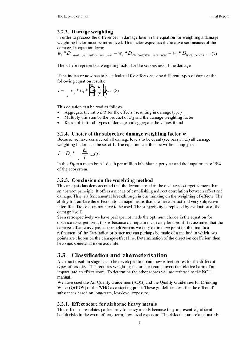
The Eco-indicator 95 Final Report
31
3.2.3. Damage weightingIn order to process the differences in damage level in the equation for weighting a damage
weighting factor must be introduced. This factor expresses the relative seriousness of the
damage. In equation form:
w D w D w Ddeath per million per year1 2 3* * *_ _ _ _ _1 5%_ecosystem_impairment smog_periods= = .... (7)
The w here represents a weighting factor for the seriousness of the damage.
If the indicator now has to be calculated for effects causing different types of damage the
following equation results:
I w DE
Tj
j
ki
ii j
=FHG
IKJ
* * ......(8)
This equation can be read as follows:
• Aggregate the ratio E/T for the effects i resulting in damage type j
• Multiply this sum by the product of Dk and the damage weighting factor
• Repeat this for all types of damage and aggregate the values found
3.2.4. Choice of the subjective damage weighting factor wBecause we have considered all damage levels to be equal (see para 3.1.5) all damage
weighting factors can be set at 1. The equation can thus be written simply as:
I DE
Tk
i
ii
= * ....(9)
In this Dk can mean both 1 death per million inhabitants per year and the impairment of 5%
of the ecosystem.
3.2.5. Conclusion on the weighting methodThis analysis has demonstrated that the formula used in the distance-to-target is more than
an abstract principle. It offers a means of establishing a direct correlation between effect and
damage. This is a fundamental breakthrough in our thinking on the weighting of effects. The
ability to translate the effects into damage means that a rather abstract and very subjective
intereffect factor does not have to be used. The subjectivity is replaced by evaluation of the
damage itself.
Seen retrospectively we have perhaps not made the optimum choice in the equation for
distance-to-target used; this is because our equation can only be used if it is assumed that the
damage-effect curve passes through zero as we only define one point on the line. In a
refinement of the Eco-indicator better use can perhaps be made of a method in which two
points are chosen on the damage-effect line. Determination of the direction coefficient then
becomes somewhat more accurate.
3.3. Classification and characterisationA characterisation stage has to be developed to obtain new effect scores for the different
types of toxicity. This requires weighting factors that can convert the relative harm of an
impact into an effect score. To determine the other scores you are referred to the NOH
manual.
We have used the Air Quality Guidelines (AQG) and the Quality Guidelines for Drinking
Water (QGDW) of the WHO as a starting point. These guidelines describe the effect of
substances based on long-term, low-level exposure.
3.3.1. Effect score for airborne heavy metalsThis effect score relates particularly to heavy metals because they represent significant
health risks in the event of long-term, low-level exposure. The risks that are related mainly
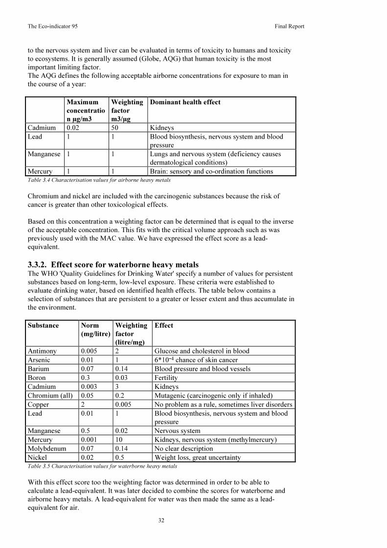
The Eco-indicator 95 Final Report
32
to the nervous system and liver can be evaluated in terms of toxicity to humans and toxicity
to ecosystems. It is generally assumed (Globe, AQG) that human toxicity is the most
important limiting factor.
The AQG defines the following acceptable airborne concentrations for exposure to man in
the course of a year:
Maximum
concentratio
n µg/m3
Weighting
factor
m3/µg
Dominant health effect
Cadmium 0.02 50 Kidneys
Lead 1 1 Blood biosynthesis, nervous system and blood
pressure
Manganese 1 1 Lungs and nervous system (deficiency causes
dermatological conditions)
Mercury 1 1 Brain: sensory and co-ordination functionsTable 3.4 Characterisation values for airborne heavy metals
Chromium and nickel are included with the carcinogenic substances because the risk of
cancer is greater than other toxicological effects.
Based on this concentration a weighting factor can be determined that is equal to the inverse
of the acceptable concentration. This fits with the critical volume approach such as was
previously used with the MAC value. We have expressed the effect score as a lead-
equivalent.
3.3.2. Effect score for waterborne heavy metalsThe WHO 'Quality Guidelines for Drinking Water' specify a number of values for persistent
substances based on long-term, low-level exposure. These criteria were established to
evaluate drinking water, based on identified health effects. The table below contains a
selection of substances that are persistent to a greater or lesser extent and thus accumulate in
the environment.
Substance Norm
(mg/litre)
Weighting
factor
(litre/mg)
Effect
Antimony 0.005 2 Glucose and cholesterol in blood
Arsenic 0.01 1 6*10-4 chance of skin cancer
Barium 0.07 0.14 Blood pressure and blood vessels
Boron 0.3 0.03 Fertility
Cadmium 0.003 3 Kidneys
Chromium (all) 0.05 0.2 Mutagenic (carcinogenic only if inhaled)
Copper 2 0.005 No problem as a rule, sometimes liver disorders
Lead 0.01 1 Blood biosynthesis, nervous system and blood
pressure
Manganese 0.5 0.02 Nervous system
Mercury 0.001 10 Kidneys, nervous system (methylmercury)
Molybdenum 0.07 0.14 No clear description
Nickel 0.02 0.5 Weight loss, great uncertaintyTable 3.5 Characterisation values for waterborne heavy metals
With this effect score too the weighting factor was determined in order to be able to
calculate a lead-equivalent. It was later decided to combine the scores for waterborne and
airborne heavy metals. A lead-equivalent for water was then made the same as a lead-
equivalent for air.

The Eco-indicator 95 Final Report
33
3.3.3. Carcinogenic substancesThe 'AQG' does not provide any acceptable levels but calculates the probability of cancer at
a level of 1 µg/m3. In the table below this probability is expressed as the number of people
from a group of 1 million who will contract cancer at this exposure level.
Probability of
cancer at
1 µg/m3
Weighting
factor for
PAH
equivalent
Type of cancer
Arsenic 0.004 0.044 General, also mutagenic effects
Benzene 0.000001 1.1 * 10-5 Leukaemia
Nickel 0.04 0.44 Lung and larynx
Chromium 6 0.04 0.44 Various incl. lung, also mutagenic
effects
PAH
(Benzo[a]pyrene)
0.09 1 Lung cancer, but also other forms
Table 3.6 Characterisation values for carcinogenic substances
The PAH group contains a large number of substances. Benzo[a]pyrene has been chosen as
a representative. An improvement in this score would be possible if account could be taken
of a substance's persistence. This applies in particular to the group of PAHs.
The inclusion of asbestos can also be considered. The difficulty here is that asbestos
emissions cannot be expressed sensibly in a unit of weight. The number and type of fibres is
of decisive importance.
3.3.4. Winter smogOnly dust and SO2 play a role with this effect. The 'Air Quality Guidelines' specify a level
of 50 µg/m³ for both substances. The weighting factors are equal; we have chosen 1. An
improvement is possible by taking account of the average persistence time of the
components. There was a lack of data on this. The definition of the term could also be
improved.
3.3.5. PesticidesPesticides cause a number of problems, including:
• Groundwater becomes too toxic for human consumption.
• Biological activity in the soil is impaired, resulting in damage to vegetation.
This means that account must be taken of both ecotoxicity and human toxicity in the effect
score weighting. A distinction must be drawn between: disinfectants, fungicides, herbicides
and insecticides.
The NOH classification provides an extensive list of weighting factors for pesticides based
on their ecotoxic effect. We considered using these, but it proved not to be possible because
no adequate normalisation data were available for these substances. The normalisation data
are based on an aggregate of the amount of active ingredient without further weighting of
the toxicity itself.
A further improvement in this effect score is possible by weighting the substances for their
persistence. Some pesticides remain active for years, while others have almost disappeared
after one day.
3.3.6. UncertaintyIn the WHO publications estimates of the uncertainties are made in a number of places. As a
rule the greatest uncertainty arises from extrapolation of animal experiments to humans
(generally one order of magnitude). Other uncertainties arise because the exposure and the

The Eco-indicator 95 Final Report
34
resulting consequences are only measured in a small number of test subjects and always
retrospectively. Here too the error can easily be one order of magnitude.
3.3.7. ConclusionThe NOH classification remains the basis for the Eco-indicator; only the term "toxicity" is
defined in greater detail. These new classifications fit much better with the description of
the environmental problems in Europe. This makes it possible to carry out a weighting for
each type of toxicity.
3.4. NormalisationStrictly speaking, normalisation values are unnecessary in a distance-to-target evaluation
because they are omitted from the weighting equation (1). However, it is seen to be
important for two reasons to continue to include these values.
• Normalisation greatly increases our understanding of the weighting. Normalisation is
a more or less objective step that illustrates what effects are relatively strongly
represented in the effect scores.
• In much of the literature objectives are specified as reduction factors. In other words,
the factor by which an effect must be reduced is specified, without stating which
absolute value must be achieved.
It was intended at the outset of the project to use the normalisation values from the recent
CML publication by Guinée [19]. The report is specially intended to calculate normalisation
values that fit the NOH effect definition. The figures are based on recordings of emissions
(fourth round) based on 1988. This list contains the total emissions in the Netherlands in
1988. A conversion factor was applied to translate these values into world effect values. To
do this, all the figures were multiplied by 100 because the Dutch economy represents
approximately 1% of world-wide GNP. An exception was made for greenhouse gases and
ozone-layer-depleting substances, for which actual international figures were used (derived
from the IPPC16). This raised a number of difficulties:
• The Dutch economy is certainly not a reflection of the world economy. In the
Netherlands there is a relatively large amount of base chemical processes and
transportation, but relatively little consumer goods production. The emissions pattern is
specific to our economy, and it is dangerous to scale this pattern up to a world level.
• The publication of emissions recordings indicates itself that it is incomplete. Sectors
such as agriculture are insufficiently covered.
• The Eco-indicator is based on a European scale.
We also investigated to what extent the characterisation of effects agrees with the
descriptions of the most important environmental problems. It might be expected that a
substance that makes a major contribution to a world effect score would also have to be
described in other literature sources as an importance cause of this effect.17
The result of this analysis cannot always be explained. It turns out that substances that make
a major contribution to the NOH effect score actually scarcely appear in the specialist
environmental literature on impairment of health and ecosystems.
16 IPCC: Intergovernmental Panel on Climate Change
17 It is therefore seen that when applying the NOH classification to the overall total of European
emissions phenol emissions must be regarded as the most significant European human toxicity
problem. Cobalt remains very dominant in terms of ecotoxicity. This result does not fit with the
description of environmental problems in Europe. In most of the literature carcinogenesis, heavy
metals such as cadmium, mercury, lead etc. are noted as major problems. Phenol almost cannot
become a major problem because it has a half life of 6 weeks and therefore can hardly accumulate
in the environment.

The Eco-indicator 95 Final Report
35
3.4.1. European normalisation valuesWhen defining target values use was made of data that refer to the whole of Europe, apart
from the former USSR. We searched for data for this area in various publications. The
countries studied can be divided into two groups:
Western Europe: Austria, Belgium, Denmark, Finland, France, Germany18, Greece, Iceland,
Ireland, Italy, Luxembourg, Netherlands, Norway, Portugal, Spain, Sweden, Switzerland,
UK.
Eastern Europe: Bulgaria, Czechoslovakia19, Hungary, Poland, Romania and Yugoslavia20
3.4.2. Data sourcesThe data were taken from various sources. They refer to anthropogenic emissions. This
implies that emissions from natural sources are not included. The table below lists the
sources used in determining the normalisation values.
Source Title and publisher
1 The Environment in Europe and North-America, Annotated Statistics 1992,
Economic Commission for Europe, United Nations Publication [37]
2 Corinair 1990 , provisional results [6]
3 Environmental Statistics 1991, Eurostat, [11]
4 The Environment in Europe: a Global Perspective, RIVM. [33]
5 General Environmental Statistics 1992], CBS (NL), [5]
6 Industrial emissions in the Netherlands No. 14, September 1993, [23]
7 CFC commission, a collaborative project by Government and industry
Annual report 1993, [4]Table 3.7 Data sources for normalisation values
Sources 1, 2, 3 and 4 provide information relating to a large area, mostly on a regional basis.
Sources 5, 6 and 7 on the other hand are specific to the Dutch situation.
With regard to source 2 it may be noted that the data are not yet complete. The final version
will be published in spring 1995.
3.4.3. Extrapolation of missing impactsWhere data were missing for one or several countries a total emission was extrapolated.
This extrapolation is based on a country's energy consumption. It is anticipated that a
country's energy consumption will best reflect the country's industrial structure and thus the
emissions pattern. Because Eastern and Western Europe have a completely different
infrastructure these areas have been calculated separately and later re-combined. A
spreadsheet that is included as Appendix 2 was used for the calculations.
The table below lists the normalisation values. The data per European head of population
(497 million inhabitants) are given in the penultimate column.
18 Data for West and East Germany combined.
19 Data refer to the former Czechoslovakia as a whole; no division into the Czech Republic and
Slovakia.
20 Data specified for the area of the former Yugoslavia; no sub-division by separate republics.

The Eco-indicator 95 Final Report
36
Unit Western
Europe
Eastern
Europe
Total Per head
of the
population
Uncer-
tainty
Greenhouse effect GWP kg 4.8E+12 1.7E+12 6.5E+12 1.31E+04 small
Ozone layer depletion ODP kg 3.7E+08 9.4E+07 4.6E+08 9.26E-01 large
Acidification AP kg 3.5E+10 2.1E+10 5.6E+10 1.13E+02 small
Eutrophication NP kg 1.4E+10 5.1E+09 1.9E+10 3.82E+01 mod.
Heavy metals Pb equiv. kg 2.1E+07 5.9E+06 2.7E+07 5.43E-02 large
Carcinogens PAH equiv. kg 4.3E+06 1.1E+06 5.4E+06 1.09E-02 large
Winter smog SO2 equiv. kg 2.3E+10 2.3E+10 4.7E+10 9.46E+01 small
Summer smog POCP kg 7.0E+09 1.9E+09 8.9E+09 1.79E+01 large
Pesticides active ingr. kg 3.8E+08 9.8E+07 4.8E+08 9.66E-01 large
Table 3.8 Normalisation values.
3.4.4. UncertaintyA number of figures are based on only small data sets. The uncertainty relating to these
effects is therefore fairly large. Determining the degree of uncertainty is not a simple matter.
There are various error sources:
• Errors in the statistics. It seems not improbable that errors of 10% have occurred in the
reported figures. This is sometimes apparent from differences between sources relating
to the same country and year.
• Errors arising from extrapolation. Some figures are computed mainly from Dutch
figures. Distortions to the order of several tens of percents can occur.
• Incomplete emissions list per effect. The statistics do not contain all the substances that
contribute to an effect. We have ensured that all important substances are included,
insofar that it is clear which are the relevant substances. The error resulting from this is
estimated to be 10-20% in some cases.
It is difficult to underpin the percentage estimations given above. There is therefore
uncertainty about the uncertainty.
The subjects to which this relates are:
• Ozone layer depletion. The score is based to an extent of 43% on Dutch data. These data
are in themselves already unreliable because the use of CFCs is falling rapidly. The
reference date thus plays an important role. We chose 1990. We estimate that the margin
of uncertainty may be of the order of 100%.
• Heavy metals and carcinogens. Dutch figures have been used almost entirely for this. It
is anticipated that it is precisely these emissions that will be relatively high in Eastern
Europe because of the use of leaded petrol and coal. With reference to carcinogens the
PAH group represents an important problem. Many sources do not indicate which
substances should be included. The margin of uncertainty may be ±100%.
• Pesticides. These data are based on average Western European values and then scaled
up to Eastern Europe. The uncertainty could be of the order of 50%.
The other effects are based on a relatively large number of data. We expect the uncertainty
here to be of the order of ±10%. However, these uncertainties cannot be backed up in any
way at all. They are based solely on estimates.
3.5. Target valuesThe target values were mainly taken from an extensive scenario study carried out by the
RIVM for the GLOBE Europe organisation. We will refer to this as the Globe report [33].
The report describes the damage caused by each effect, using a large number of maps.
Furthermore, it describes what the effects would be of a couple of scenarios. We have not
used these scenarios themselves, but the underlying data. Although extensive reference lists
are provided it is unfortunately not always clear on what statements in the report are

The Eco-indicator 95 Final Report
37
founded and what the uncertainties are. A request for clarification of a number of points was
made during discussions with the editor of the report, Mr. J.P. Hetteling.
To aid comprehension of the following survey it is urgently recommended that this paper be
consulted. We will only deal here with the conclusions that we have drawn from the report.
In addition to the Globe report we also used the Air Quality Guidelines [2] and the Quality
Guidelines for Drinking Water [38] that have been developed by a large team of experts
under commission from the WHO. We used this to supplement the Globe report in a few
areas.
3.5.1. Greenhouse effectAt the moment temperatures are rising by 0.2°C per decade. Under current policies this
increase will rise to 0.3°C per decade. The consequence is a significant temperature change
by 2050. In Northern and Eastern Europe the winters will be more than 5°C warmer, and in
Southern Europe the summers will be 4°C warmer. Those areas in particular that have no
other systems in their vicinity that can exist in such a climate will suffer serious damage.
This will affect approx. 20% of Europe.
The Globe report provides sufficient information to estimate that less than 5% of the
ecosystems will be impaired if the greenhouse effect is reduced by a factor of 2.5.
3.5.2. Ozone layer depletionIn accordance with the Montreal Protocol and its London amendment all CFC emissions
must be reduced to zero by the year 2000. For the less persistent HCFCs it has been agreed
that the contribution may not exceed 2.6% of the total adverse effect of CFCs in 1989. The
use of these substances too is to be phased out by 2015.
If this happens, the annual total of fatalities per million inhabitants in Europe will first rise
from approximately 1 to 2 and then fall to 1 death per year per million. It does not yet seem
directly necessary to reduce all HCFC emissions to zero because the norm (2 ppbv) will be
achieved, even if after 2100. For these gases the target reduction is linked to the greenhouse
effect21.
Based on this reduction for greenhouse gases, we therefore provisionally assume that a
reduction target of 60% applies to HCFCs. On the premise that HCFCs are currently
responsible for 2.6% of ozone layer depletion it can be estimated that this reduction will
cause ozone layer depletion to fall to 1% of its present level. The reduction factor is
therefore 100. There is a great deal of uncertainty about this figure.
3.5.3. AcidificationThere is a great variety in Europe in the ability of ecosystems to withstand acid loads. In
Scandinavia, for example, problems can occur with deposits of as little as 100 eq/ha.yr,
while in some places in the Netherlands and Germany the soil can be subjected to deposits
of more than 2000 eq/ha.yr. The actual deposit reaches its highest level, however, in Central
Europe, particularly as a result of the use of lignite. If the deposit and capacity are compared
with each other there prove to be major problems particularly in England, the Benelux
countries, Germany, Poland, the Czech Republic and Slovakia [9].
A provisional estimate based on the information available reveals that the reduction must be
of the order of a factor of 10 to keep ecosystem impairment below 5%. A value of 10 was
ultimately chosen.
21 Conversely, a marked reduction in the greenhouse effect will also be achieved by the elimination of
CFCs since CFCs are responsible for 24% of this effect. Elimination of CFCs will therefore yield a
24% reduction in the greenhouse effect.

The Eco-indicator 95 Final Report
38
Fig. 3.2 Example of an acidification map from the RAINS program [30]
3.5.4. EutrophicationEutrophication is seen in the Globe report primarily as the problem of excessive use of
fertilisers by agriculture as a result of which nitrates leach out and poison groundwater
supplies. The problem is at its greatest in the Benelux countries, North-Rhine Westphalia
and the Po valley region (approx. 200 kg P-eq/ha.yr).
The NOH manual refers mainly to eutrophication via air and water emissions. These rarely
contribute more than 10% of the amount of fertiliser applied by farmers. In uncultivated
biotopes, however, this eutrophication can have a serious adverse effect on biodiversity.
In describing the level of eutrophication in rivers and lakes it is assumed that the critical
value for phosphates is 0.15 mg/l and for nitrates 2.2 mg/l. At these values no problems of
eutrophication occur. In the rivers Rhine, Schelde, Elbe, Mersey and Ebro, however, these
values are exceeded more than 5 times. This means that the emissions must be reduced by a
factor of 5.
3.5.5. Summer smogA hundred years ago the ozone concentration, averaged over the whole year, was approx.
10 ppb. At present it is 25 ppb. This is approximately the maximum acceptable level. Above
30 ppb, for example, crop damage can occur.
The major problem is not determined by the average figures but by the summer peaks which
can reach more than 300 ppb. To reduce the occurrence of this type of dangerous peaks by
90% it is necessary to reduce VOCs and NOx by 60-70%. A reduction factor of 2.5 is
appropriate.
3.5.6. Heavy metalsLead concentrations in Central Europe are very high, particularly in the soil and water. In
towns and cities the airborne concentration is also high, particularly because of the use of
leaded petrol. For adults the Air Quality Guidelines specify a limit of 0.5-1 µg/m3 in the air.
According to Globe this value is frequently exceeded several times over. Globe notes in
passing (without reference) that average lead concentrations in Poland are 20 µg/m3.
Eating locally grown vegetables would result in a blood lead level that is ten times too high.
Lead levels in blood of 150-400 µg/l have been found in children. Such readings also
occurred 30 years ago in the West, but not any more. Now the values are 5 to 10 times
lower. There is thought not to be a no-effect-level for exposure for children. Above 100 µg/l
clear reductions in learning ability can be measured.

The Eco-indicator 95 Final Report
39
Thus although it is plausible that this pollution has a clearly measurable effect on human
health it is not easy to calculate a general reduction percentage for lead. The best estimate is
a reduction by a factor of 5-10. We have taken a figure of 5 for heavy metal emissions to air.
Agriculture (fertiliser) is the major source of cadmium deposition. The average deposition
rate is 0.6-0.67 g/ha.yr on grassland and 3.4-6.8 g/ha.yr on arable land. The Southern
Netherlands holds the record with a deposit of 7.5-8.5 g/ha.yr. Furthermore, approx. 14% is
distributed via the air (see "3.5.7 Winter smog" below).
This leaching is calculated in the Globe report for the Rhine. A detailed calculation makes a
convincing case for the necessity to reduce cadmium emissions by 80-85%. In some other
rivers such as the Elbe, cadmium contamination is substantially greater, and the required
target will perhaps have to be set even higher. For the moment we are continuing with a
target reduction by a factor of 5 for heavy metals in water and air.
3.5.7. Winter smogThe most important sources of this problem which occurs mainly in Eastern Europe are SO2and SPM (suspended particle matter, or fine dust and soot particles). NOx, organic
substances and CO are also involved to a lesser extent. The dust particles can also contain
heavy metals.
This form of smog achieved notoriety in 1952 when it caused an estimated 4000 deaths in
London. The SO2 and SPM concentrations reached values of 5000 µg/m3. In Southern
Poland and Eastern Germany average readings of 200 µg/m3 still occur. The Air Quality
Guidelines specify a limit of 50 µg/m3 for long-term exposure to both SPM and SO2. Based
on this, a reduction of 75% would be necessary.
Globe estimates that a reduction in SO2 emissions of more than 80% is necessary to
eliminate by and large the occurrence of occasional smog periods. No target is proposed for
SPM because it is not well defined or well measured22. A factor of 5 is taken as a reduction
target.
3.5.8. Carcinogenic substancesGlobe also provides some data on the distribution of carcinogenic substances. The main
substances involved are polyaromatic hydrocarbons (PAHs), of which benzo[a]pyrene in
particular is an important example. This occurs, among other places, in coke furnaces and in
(diesel) engines. In fact the problem is only relevant in urban areas.
Globe specifies a value of 0.8-5 ng/m3 voor Northern European towns and cities. The Air
Quality Guidelines specify a value of 1 ng/m3 in American cities without coke furnaces in
the vicinity and 1-5 ng/m3 in cities with coke furnaces. In European towns and cities in the
60s when open coal fires were still very widely used, the average concentrations were in
excess of 100 ng/m3. In Eastern Europe the values are still high because of the use of coal-
fired heating systems. As a point of comparison, a room in which a lot of people are
smoking can contain 20 ng/m3.
The Air Quality Guidelines specify a threshold concentration van 0.01 ng/m3 at which 1
cancer case per million inhabitants per year will still occur. This criterion cannot be
compared straightforwardly with the criterion for ozone layer depletion because not all the
cancer cases are terminal. In addition, only about 1/3 of the population of Europe lives in
towns or cities23. If we assume that one in every three cancer cases is terminal and if we take
only the urban population the risk of death is about ten times lower. Based on these
considerations there would be one death per year per million inhabitants at a concentration
of 0.1 ng/m3.
22 In the NOH manual there is no weighting factor for SPM in characterising human toxicity.
23 Eurostat [11], estimate based on data for 6 EU member states

The Eco-indicator 95 Final Report
40
Assuming a background concentration of 1 ng/m3 in towns and cities without coke furnaces
(Western European towns and cities in particular) a reduction by a factor of 10 could be
estimated.
3.5.9. PesticidesLeaching of pesticides threatens groundwater sources throughout the EU. In 65% of the EU
the groundwater is contaminated above the EU norm (0.5 µg/litre). The norm is exceeded
tenfold in 25% of the EU. This occurs in 20% of the land area of Eastern Europe. A
reduction by a factor of 25 is necessary to ensure that the norm is exceeded in less than 10%
of Europe.
3.5.10. UncertaintyThere is uncertainty about every single value cited. A number of factors have an important
role to play in this:
• The degree to which the criterion fits with the effect definition. This problem is reduced,
but not entirely resolved, by redefining the effects. The uncertainty associated with this
point cannot be quantified.
• The uncertainty over the occurrence of the effect24. These uncertainties are difficult to
quantify.
• Uncertainty in the exposure of ecosystems and people. All kinds of local circumstances
and human behaviour can result in substantial variations in the actual exposure to a
substance .
• Intereffect combinations. It is known that some substances when in combination
reinforce each other or work against each other25.
• The derivation of the target values themselves. In various places in the above
description it has been stated that there are uncertainties.
It is difficult to determine the magnitude of the uncertainty. In toxicological studies it is
quite normal to work with uncertainties of several orders of magnitude. Nevertheless data
with such uncertainties are used in order to establish standards and regulations.
In general we believe that the uncertainties in the reduction factors are of the order of
several tens in percentage terms, but we are unable to back this estimate up.
3.5.11. Summary of the weighting factorsThe table below summarises the figures and the values used in determining them.
24 Example: with the greenhouse effect a marked rise in temperature is expected. Recent calculations,
however, predict a temperature reduction in Europe as a result of the disappearance of the warm
Gulf Stream because of higher temperatures at the North Pole.
25 Examples: nickel in combination with cigarette smoke is much more dangerous than nickel in
isolation. Because of SO2 clouds become whiter and their reflecting capacity is increased; the
outcome is that it gets colder on Earth.

The Eco-indicator 95 Final Report
41
Character-
isation
Reduction
factor
Criterion
Greenhouse
effect
NOH
(IPCC)
2.5 0.1° per decade, 5% ecosystem impairment
Ozone layer
depletion
NOH
(IPCC)
100 Probability of 1 death per year per million people
Acidification NOH 10 5% ecosystem impairment
Eutrophication NOH 5 Rivers and lakes, impairment of an unknown number
of aquatic ecosystems? (5% ecosystem impairment?)
Summer smog NOH 2.5 Occurrence of smog periods, health complaints,
particularly among asthma patients and old people.
Occurrence of agricultural damage
Winter smog Air Quality
Guidelines
5 Occurrence of smog periods, health complaints,
particularly among asthma patients and old people
Pesticides Active
ingredient
25 5% ecosystem impairment
Heavy metals
in air
Air Quality
Guidelines
5 Lead level in children's blood, limited life
expectancy and learning ability in an unknown
number of people
Heavy metals
in water
Quality
Guidelines
for Water
5 Cadmium content in rivers, ultimately also effect on
people (see air)
Carcinogenic
substances
Air Quality
Guidelines
10 Probability of 1 death per year per million people.
Table 3.9 Summary of the weighting factors
The last column indicates the criterion on which the target value is based. The damage types
defined previously are recognisable here.
ConclusionThe Eco-indicator weighting method is a refinement of the LCA method using published
guidelines, the NOH manual and the SETAC Code of Practice. The evaluation stage is based
on the distance-to-target principle, and the normalisation stage is based on European data
(excluding the former Soviet Union). The decision in favour of this principle was made in
phase 1 after a detailed evaluation of other principles. During the project is became clear
that this principle leaves a lot of room for interpretation and that improvements in the
principle are possible in the event of future developments.
A number of conclusions can be drawn with regard to the methodology:
• An Eco-indicator cannot be developed without clearly defining and demarcating the
term "environment" or "eco". Such a definition and demarcation were developed during
this project. The Eco-indicator applies only to environmental affects that damage
ecosystems or human health on a European scale. Other effects are not covered.
• In evaluating environmental effects the damage caused by the effect is a determining
factor for the seriousness of an effect. It is inevitable that the damage-effect relation will
be used when developing a weighting method. The direction coefficient of the damage
effect function is in principle the weighting factor.
• Distance-to-target as a weighting principle does establish a link between damage and
effect, but this effect is not ideal in its present form because it only defines one point on
the damage-effect function. This means it is not possible to determine the slope of this
function directly. In the future it seems that it will be possible to improve the weighting
principle by defining two points on the damage-effect function. Such a method requires
double the quantity of data.

The Eco-indicator 95 Final Report
42
• There are various types of environmental damage. For this reason it is necessary to
weight different types of damage. Subjectivity is inevitable with such a weighting. In
relative terms, however, it is much easier to weight damage subjectively than effects.
• The Eco-indicator is based on the subjective assumption that the 5% ecosystem
impairment is equivalent to the death of one person per million per year. Different
assumptions would result directly in different weighting factors.
• The difference of view that seemed so important in the first phase of this project as to
whether the current or the target value should be normalised has proved to be much less
relevant than first thought.
• Raw materials depletion and the space required for final waste cannot be correlated with
a form of environmental damage. After all, no ecosystems are impaired and no-one dies
as a result of such depletions. This means that it is not easy to weight the seriousness of
raw materials depletion. The extraction of raw materials and the generation of waste are
evaluated, however, in that the impacts as a result of the extraction of raw materials and
the processing of waste are completely evaluated. It ought to be possible to develop a
separate indicator for evaluating raw materials depletion.
• The uncertainties in the results of the weighting method are still large. This applies both
to normalisation and to weighting. It could even be that the normalisation values contain
even more uncertainties than the weighting factors. It seems to be very sensible to draw
up a new inventory of the available normalisation data after some time.

The Eco-indicator 95 Final Report
43
4. Calculation of the Eco-indicators
The development of 100 Eco-indicators for materials and processes ultimately required 100
LCAs to be carried out. This means that the inventory phase was run 100 times.
The NOH manual and the SETAC Code of Practice state in general terms the requirements
with which an inventory phase has to comply. The most important requirement is that the
choices, the system boundaries and the allocation principles must all be clearly stated. There
is no straightforward receipt for the inventory stage. The researcher has to make a large
number of choices when searching for and interpreting data. These choices can greatly
influence the result.
Both manuals rightly assume that the way in which the inventory phase is carried out
depends among other things on the objective. Before the inventory phase can be carried out
the objective must be carefully defined. Based on this objective certain methodological
choices can be formulated. Explicitly stating these choices in advance will prevent the
researcher from making different assumptions ad hoc for various processes or will prevent
him, even worse, from working towards a result.
4.1. Definition of the objectiveThe Eco-indicators (the 100 figures) are intended for use within companies, particularly as a
decision-making support tool for product design or management decisions. It is primarily a
means of taking account of environmental aspects in a decision if there is little time to carry
out detailed analyses.
The Eco-indicator is intended to take generic decisions on materials, working principles and
life cycles. The indicators are not intended for use in controlling the purchase of materials
(selection between two aluminium suppliers) or in taking important investment decisions.
This means that the user does not know where the impacts will occur.
The users in this project are companies operating on the international market. This means
that the indicator must also be relevant outside the Netherlands. Europe is an acceptable
scale for the companies involved.
This objective has a number of other important consequences:
• The data must be generally applicable. The figure for aluminium, for example, must be
based on the average emissions in the production of aluminium.
• The data must be gathered such that it is possible to compare the indicators well with
each other. Mutual comparability of the figures is more important than the absolute
value. All data must therefore be gathered in the same way.
• The inventory method must fit as well as possible with the current working method used
by LCA researchers.
The consequences of these statements are explained in greater detail below.
4.1.1. Functional unitFor an LCA it is of great importance to define precisely which product is actually being
studied. Particularly when comparing two products it is important to ensure that the products
are actually equivalent and perform the same task.
In the Eco-indicator project the functional unit is somewhat less visible because no products
are analysed over their entire life cycle. The aim is only to produce the building blocks for
analysing product life cycles. The designer can establish his own functional unit and carry
out an LCA with the indicators. What is required, therefore, is to develop an LCA kit of
compatible LCA modules, each with its own indicator value. The are five types of LCA
modules:
1. Material production
2. Material processing
3. Energy conversion or generation
4. Transport
5. Waste processing
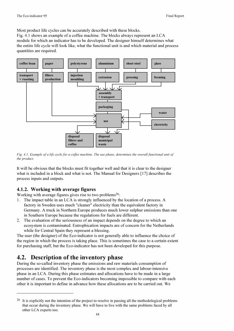
The Eco-indicator 95 Final Report
44
Most product life cycles can be accurately described with these blocks.
Fig. 4.1 shows an example of a coffee machine. The blocks always represent an LCA
module for which an indicator has to be developed. The designer himself determines what
the entire life cycle will look like, what the functional unit is and which material and process
quantities are required.
assembly
polystyrene
injection
aluminium
extrusion
+ transport
disposal
municipal
waste
electricity
disposal
use
paper
filters
production
sheet steel
pressing
glass
forming
filters and
coffee bean
transport
+ roasting
packaging
water
moulding
coffee
Fig. 4.1. Example of a life cycle for a coffee machine. The use phase, determines the overall functional unit of
the product.
It will be obvious that the blocks must fit together well and that it is clear to the designer
what is included in a block and what is not. The Manual for Designers [17] describes the
process inputs and outputs.
4.1.2. Working with average figuresWorking with average figures gives rise to two problems26:
1. The impact table in an LCA is strongly influenced by the location of a process. A
factory in Sweden uses much "cleaner" electricity than the equivalent factory in
Germany. A truck in Northern Europe produces much lower sulphur emissions than one
in Southern Europe because the regulations for fuels are different.
2. The evaluation of the seriousness of an impact depends on the degree to which an
ecosystem is contaminated. Eutrophication impacts are of concern for the Netherlands
while for Central Spain they represent a blessing.
The user (the designer) of the Eco-indicator is not generally able to influence the choice of
the region in which the process is taking place. This is sometimes the case to a certain extent
for purchasing staff, but the Eco-indicator has not been developed for this purpose.
4.2. Description of the inventory phaseDuring the so-called inventory phase the emissions and raw materials consumption of
processes are identified. The inventory phase is the most complex and labour-intensive
phase in an LCA. During this phase estimates and allocations have to be made in a large
number of cases. To prevent the Eco-indicators becoming impossible to compare with each
other it is important to define in advance how these allocations are to be carried out. We
26 It is explicitly not the intention of the project to resolve in passing all the methodological problems
that occur during the inventory phase. We will have to live with the same problems faced by all
other LCA experts too.

The Eco-indicator 95 Final Report
45
have made a description of the way in which the inventory phase must be conducted in
advance.
The description below of the working method during the inventory phase represents the
ideal. The picture is determined by the objectives described above. In practice we had to
deviate from this ideal, because there were simply no reliable data available. In some cases
we dispensed with the calculation of an indicator. This description can also serve as a guide
if new indicators have to be determined.
A large number of problems in the inventory phase are described in the LCA literature.
However, almost all the problems can be grouped under a number of headings:
System
boundaries
problems
No single product forms a completely isolated product system, independent
of other products. Capital goods and auxiliary products are almost always
required to manufacture, transport, use and dispose of a product. Because it
is impossible in practice to take account of all these interactions, boundaries
must be set for the product system.
Allocation
problems
Many processes result in by-products in addition to a main product.
Furthermore, in the case of recycling, the same material is used in several
product cycles. In these cases the environmental impacts of a process or
cycle must be allocated to these products.
Choice of
Technology
Particularly with an Eco-indicator it is important to assume the same state of
the technology for all the processes.
Time and
space
The location where a process takes place has a marked influence not only on
the impact table but also on the evaluation of the seriousness of the effects.
With durable products there is also the problem that use and disposal
processes will not take place now but over an extended period. It is not
known what the state of the art will then be.Table 4.1 Summary of complications in the inventory phase.
4.2.1. System boundariesA number of rules apply for all types of data, while others apply specifically to material
production, transport etc.
In principle all processes are included from raw material extraction to the final process,
which results in the outcome described in the material and process definition. However, the
following are exceptions to this:
• Production, maintenance and disposal of capital goods. Capital goods are defined to
include fixed installations, transport systems and such like that are seen as investment
goods in an economic sense. Dies are also included. Maintenance primarily covers
major inspections and repairs. Emissions of consumed auxiliary materials such as fuels,
lubricants, quick-wearing parts and such like are included in the system.
• Human labour, transport of people etc. Heating and lighting of the production processes,
however, are not included because they can often not be distinguished from the other
processes in a factory.
• Risks and emissions resulting from accidents and major malfunctions.
In addition to these general rules, a number of specific rules apply.
4.2.1.1. Material production
The starting point is the extraction of raw materials. The finishing point is the process that
produces the material in the quality and form for supply as described in the material and
process definition.
The process tree incorporates all transport for the material and auxiliary items, including the
industrial packaging. Mining processes are fully included, even if they take place outside
Europe.

The Eco-indicator 95 Final Report
46
4.2.1.2. Energy generation
All raw material extraction, distribution and manufacturing processes must be included up
to the moment that the fuel is ready for sale in Europe.
4.2.1.3. Transport
An important problem is the question of to what extent the transport means are used to their
full load- or volume-carrying capacity, and also the question of to what extent transport
means return empty. In the list of indicators transport is given both per kilo and per volume,
for an average degree of loading; this takes account of transporters returning empty.
4.2.1.4. Production processes
The description of the production processes specifies the input and output of the process.
The system boundaries must be based on this.
4.2.1.5. Waste processes
The materials and processes list also contains a number of waste processing and recycling
processes. By this we mean the processes that are necessary to collect and process waste
materials or to separate and purify the materials until they are more or less pure raw
materials. Almost no experience is available with regard to carrying out LCAs for waste
processing. This will change though when the Afval Overleg Orgaan [AOO - Waste
Disposal Authority] publishes its environmental effect report on waste processing in the
Netherlands. Based on personal communications and certain draft outlines we have already
included some of these data and methodological choices in this project.
Within the Eco-indicator project there has been a great deal of information exchanged on the
allocation of useful waste processing by-products, such as heat (electricity) and reclaimed
materials (paper, scrap metal, glass etc.)27.
An important fact is that recycling may only be used in the analysis if a material is actually
going to be recycled. The fact that a product is recyclable is irrelevant. Only if the material
is actually recycled does it produce an environmental benefit. This benefit can be specified
as follows.
• If heat from incineration is collected and used for electricity production, less electricity
has to be generated elsewhere. For this reason the impacts that would arise if electricity
were generated in a different way are often deducted in an LCA. This only applies, of
course, to electricity that is actually supplied to the grid. The impacts arising from the
incineration process are taken into account.
• If scrap metal is collected and used for steel production less pig iron has to be
manufactured. The impacts that would have been necessary to manufacture this pig iron
can be deducted from the impacts arising from the collection and separation of the steel.
The same applies to aluminium.
• If waste paper is collected and used for paper production there are savings in pulp
production.
• If plastics that are sufficiently pure are collected they can be melted down and turned
into pellets that can be used for products that would otherwise be manufactured out of
new material.
• Waste glass can be used to replace new glass. Only the inputs for collection and energy
for the melting process are taken into account.
As a result of this deduction of avoided emissions some indicators for recycling and
combustion processes are negative, meaning that the emissions from the recycling process
are lower than the emissions avoided. This would mean that the environment is cleaner in
net terms as a result of a process. In fact this is not so because every process causes
27 The critical contributions and major input by Hein Sas of the CE in this field have been very
valuable, although his view has not been completely adopted.

The Eco-indicator 95 Final Report
47
contamination. The negative score for the recycling process represents the fact that the
losses from a recycling process are smaller than the benefits.
In extreme cases the indicator for the material's entire life cycle (apart from production,
transport and use processes) can be negative. Taken literally, this would mean that the
environment would become cleaner, the more products were manufactured. This seems
nonsensical. Nevertheless it was decided to accept this "error" provisionally because the
indicator's absolute value for its entire life cycle is less relevant. The main requirement is for
the designer to be able to compare various options well with each other. For this it is more
important that the differences between the indicators are determined consistently than that
the absolute value tallies. If the designer sees a negative indicator for a particular waste
processing method in the list he will be able to see that in this case the benefits of the
process are greater than the losses.
This all proves still to be a theoretical problem at present. With the current indicator values
such situations cannot occur28.
In addition to the allocation of useful by-products a number of other allocation problems
have a role to play in the analysis of waste processing systems.
• A number of emissions are material-specific (heavy metals, CO2, SOx and NOx)
• A number of emissions are process-specific (e.g. CO and dioxin)
• The emissions are filtered with varying efficiencies
The material-specific emissions are relatively easy to assign. The amount of carbon
determines the CO2 production. The proportion of heavy metals is based on average figures
for each waste fraction.
Process-specific emissions are assigned to materials on the basis of the amount of
combustion gases produced. A substance that produces a lot of flue gas on incineration is
also assigned a lot of process-specific emissions. Examples with incineration are: dioxin,
carbon monoxide and trichloroethane.
28 This problem can be illustrated by means of a greatly simplified example. Let's assume that a
designer can only choose between the following extremes.
1. A product can be made of primary or secondary materials. Let's assume that the indicator for
primary material is 20 and for secondary material 2.
2. A product can be recycled or dumped. Let's assume that the indicator for disposal is 3 and for
collection and reprocessing 2.
The choice of secondary material as the basic material is immediately rewarded with a difference
of 18 points. If the material is dumped a further 3 points are added to this. So far the problem is
straightforward.
If the material is recycled 2 points are added. However, material is also released. Because new
material is released that is actually used, less primary material needs to be manufactured elsewhere.
The saving is therefore 20 points.
If the product is made from primary material the net score is:
Primary production 20
Collection and reprocessing 2
Material avoided -20
The total score is therefore 2. This result seems logical because after use the material is returned.
Only the emissions from collecting and reprocessing are taken into account.
If the material was already secondary material a total negative score of -16 points can arise. This is
because relatively clean material is used (only 2 points) which, after recycling, avoids the
production of new material. After all, if secondary material is also recycled the demand for primary
material falls in principle. The environment would thus apparently be cleaner if this material were
used. This rather unfortunate distortion is difficult to avoid if we wish to reward the designer both
for his sensible material choice and his choice of waste process.
An alternative arises if we agree only to reward the recycling of secondary material by deducting
secondary material. (As a rule this is the same as the recycling process itselfzelf, as a result of
which the total score for recycling plus benefit is, by definition, zero). In that case a designer who
recycles previously new material receives as many points as a designer who recycles what was
already secondary material. The use of secondary material as an input is therefore not rewarded.

The Eco-indicator 95 Final Report
48
As far as filtration is concerned we have assumed that modern installations are used.
Landfill sites are assumed to be equipped with a reliable waste water purification system
(90% efficient). These landfill sites are covered after several tens of years in operation as a
result of which no further contaminated percolation water is released. The collection of
landfill gas is not assumed. A distinction is drawn between short and long carbon cycles29.
Waste incineration plants are assumed to be equipped with a modern incineration furnace
and modern flue-gas treatment system. The slag is assumed to be used as road-surfacing
materials. The leaching of heavy metals from this was derived from trials.
It is assumed that the filter residues and fly ash are treated as chemical waste. No allowance
is made for leaching.
The end of the life cycle is a certain quantity of final waste. This is inert waste that does not
need further digestion; leaching from this can be ignored.
The waste processing figures for these parameters are on the optimistic side. They are
particularly intended for application to future situations, i.e. for products with a long
lifetime. Considerably less favourable values can apply to landfill sites that are not covered
and for less modern waste incineration furnaces.
4.2.2. Geographical distribution and type of technologyWhen defining the objective the necessity of using general figures was emphasised. By
"general" we mean particularly European. This means that as far as possible the average
European electricity figures are used and the other production processes are averaged out for
Europe as much as possible. In practice this will not be easy because little is known about
processes in Southern Europe.
The other problem, namely regional differences in evaluation for an impact, is simpler as a
result. If it is not known, by definition, where an impact takes place there is also no point in
continuing with weightings on a regional basis. When defining target values and
normalisation values we will have to work with Europe as one homogeneous region.
For processes that mainly occur outside Europe, such as mining and shipping, this means
that the evaluation of the emissions is carried out on the basis of European problems; this is
not correct, but it is practical.
We have assumed technology such as has been used on average in the last 10 years in
Western Europe. This specification leaves much room for interpretation, but there seems to
be no better definition available. With regard to waste processing we have taken very up-to-
date and, in some cases, future figures. This is logical because many products will only be
disposed of in many years. Unfortunately, only Dutch figures where available in sufficient
detail and quality.
4.2.3. Allocation of multiple output processesIn the case of processes that result in more than one product the impacts must be allocated to
these different products. There are various ways of doing this. Attempts must be made to
achieve the following:
1 Allocation on the basis of the products' economic value. This means that a product that
provides 60% of the revenue is also assigned 60% of the impacts. The thought behind
this is that economic considerations determine whether a process takes place. One
advantage of this approach is that a distinction is automatically made between waste and
by-products
29 In the case of products made of organic material that have extracted CO2 from the air in the course
of the preceding decennia the CO2 and CH4 emissions are not included (CH4 arises from the
natural decomposition of organic material). With regard to the incineration of plastics for which
the CO2 extraction took place millions of years ago the CO2 emissions resulting from incineration
are assigned as appropriate.

The Eco-indicator 95 Final Report
49
2 Subtraction of avoided emissions. This is particularly applicable in allocation useful
energy. This approach is also used with the waste processes.
Only if these processes are not adequate or if the data found cannot be changed can
allocation take place in accordance with the mass ratio.
4.2.4. Data quality and completenessA number of general rules apply for the evaluation of data quality:
• The mass balance must be checked for material processing systems.
• The results must be compared with at least one other more or less comparable processes.
Any large variations must be explained.
Account was taken, of the effect definitions from the Eco-indicator method. Where data
were clearly missing estimates were made.
4.2.5. Documentation of the dataThe following data at least must be recorded for each material and process.
1. Definition of the material or process
2. Sources used
3. Type of technology, region and period, where known
4. Graphic representation of the process tree, with the system boundaries clearly shown
5. Complete impact table, with impacts divided by:
• use of raw materials (in connection with mass balance checks)
• emissions to the air
• emissions to water and soil
• final waste (in connection with mass balance checks)
6. List of variations from the ideal model described above. In every case the results of the
quality tests described above must be given:
• mass balance
• origin of the data
• comparison with other data
7. Brief discussion of the consequences of these variations for the result
8. Calculated indicator and the three most important contributors to the indicator score.
Appendix 4 in the current report gives a specification of the data sources used. The full
description of the data, according to this definition is available in the Annexe report [14].
The titles, sources and comments are in Dutch; the inventory tables are in English
4.2.6. UncertaintyDespite all the precautionary measures taken there is a fairly large degree of uncertainty in
the impact tables. These uncertainties are very difficult to quantify. Nothing is in fact known
about the distribution, but it is probably not stochastic. This makes it almost impossible to
use an uncertainty analysis. It does not seem impossible for the Eco-indicator to be
erroneous by a factor of 2 in some cases because of uncertainties in the impact table. This
estimate cannot, however, be backed up.

The Eco-indicator 95 Final Report
50
5. Use of Eco-indicators
The Eco-indicators can be used in two ways:
1. The analysis of products or ideas, with the aim of finding the most important causes of
the environmental pollution and finding opportunities for improvement.
2. The comparison of products, semi-finished products or design concepts, after which the
least environmentally polluting components can then be chosen.
The analysis of products is of particular importance at the beginning of the design process
when comparable products (reference products) are analysed. In general this analysis
provides good insight into the dominant environmental aspects for this particular type of
product. This can direct the problem definition and the list of requirements at the start of the
design process.
Specific rules-of-thumb can sometimes be developed for a type of product. In the concept
phase too, once the contours of the new design have begun to take shape, it is useful to carry
out an analysis to examine which factors are dominant and in which direction to look for
possible optimisations.
The comparison of products is of particular importance during the creative phase and in the
selection of concepts. During the creative phase there is sometimes a need for very simple
comparisons, for example between two materials. As the design progresses, so the
comparisons, become more complex.
During the project we looked at how these two functions could be supported with an
operating manual and a number of special assessment forms. Various designers at the
companies involved were interviewed regarding a number of proposals for forms and
supporting texts. It was found that the designers saw little use in extensive support or
intricate forms. There was a clear preference for a simple list of factors and a simple
assessment-form. Based on these conclusions a specifications list was formulated and a first
version of the form was drawn up.
5.1. Test workshopThe first version of the form and the list of Eco-indicators was tested during a workshop at
Philips CFT on 14 December 1994. During the workshop designers from the four companies
involved carried out a number of analyses themselves, without further instruction in
advance. During the morning session an overhead projector was analysed by four subgroups,
based on previously distributed data on the material composition and consumption of energy
and sheets. In the afternoon each of the companies involved worked on a product of its own.
At the end the results were evaluated.
The following conclusions emerged from the workshop:
• When four different groups analyse the same product they reach the same conclusions,
independently from each other. There proved to be differences on a few points:
• The missing indicator for zinc was estimated differently by the various groups.
• Very different processes (injection moulding, foil blowing and extrusion blowing)
were chosen for the production of overhead sheets. This had a fairly large effect on
the outcome, although there was agreement on the main conclusion, namely that
sheets play a dominant role. It is obviously very important for the processes to be
clearly defined. The designers' lack of familiarity with the product plays an
important role here. A designer who designs overhead projectors will know which
process is used. In the afternoon session this problem did not occur.
• Not all designers are equally good in adding numbers. In some cases the decimal
point was wrongly positioned in the result.

The Eco-indicator 95 Final Report
51
• Despite the prior warning it was easy to slip into concentrating on details of the
production phase. In the example of the overhead projector this plays only a minor role.
Once the morning session had been completed, however, most realised that the principal
need was to analyse the main features.
• Some found the manual too long, others too short. We concluded from this that we
should separate a short introduction on using the list and the form from a somewhat
more extensive description of the backgrounds and applications. Quite a number of
comments were made about the manual's style. For this reason it has now been re-
written.
The most noticeable fact was the ease with which the design teams analysed their own
products in the afternoon session. Each group was able to name the dominant factors
causing their own product to pollute the environment. These conclusions proved to fit well
with the earlier product assessments.
5.2. List of Eco-indicatorsThe list of indicators is reproduced on the following pages. The figures have been computed
with the computer program SimaPro 3.0. The figures are in fact milli-indicators. In other
words, the result of the weighting has been divided by 1000 to give figures that are easier to
handle. The unit in the following tables is thus mPt (milli Eco-indicator point). Appendix 1
shows how the indicators are composed, using a number of graphs.
A few materials that were included in the original list have since been deleted because the
inventory stage was unsatisfactory and did not meet the minimum requirements. These
include:
• A number of non-ferrous metals; no reliable data proved to be available.
• Magnetic material; data on non-ferrous metals are needed for this.
• Waste processing for aluminium. Only data on the non-ferrous fraction are known. This
fraction also contains large quantities of harmful materials such as lead. The impacts
resulting from the processing of this fraction are therefore very high; this cannot,
however, be assigned to aluminium.
• Processing of chemical waste. The impacts from this were determined too much by the
specific composition and physical form of the material to allow a general figure to be
derived.
5.3. Assessment formTwo forms have been designed to carry out the calculations by the designer. Form 1 is
primarily intended for comparing products or analysing simple products; Form 2 is intended
for analysing more complex products.

The Eco-indicator 95 Final Report
Eco-indicator values from: The Eco-indicator 95, Final Report, 17 July 1995 (NOH report 9523 and 9524) page 52
Production of metals (in millipoints per kg)
Indicator Description
Secondary aluminium 1,8 made completely of secondary material
Aluminium 18 containing average 20% secondary material
Copper, primary 85 primary electrolytic copper from relatively modern American factories
Copper, 60% primary 60 normal proportion secondary and primary copper
Secondary copper 23 100% secondary copper, relatively high score through heavy metal emissions
Other non-ferrous metals 50-200 estimate for zinc, brass, chromium, nickel etc.; lack of data
Stainless steel 17 sheet material, grade 18-8
Secondary steel 1,3 block material made of 100% scrap
Steel 4,1 block material with average 20 % scrap
Sheet steel 4,3 cold-rolled sheet with average 20% scrap
Processing of steel (in millipoints)
Indicator Description
Bending steel 0,0021 one sheet of 1 mm over width of 1 metre; straight angle
Bending stainless steel 0,0029 one sheet of 1 mm over width of 1 metre; straight angle
Cutting steel 0,0015 one sheet of 1 mm over width of 1 metre
Cutting stainless steel 0,0022 one sheet of 1 mm over width of 1 metre
Pressing and deep-drawing 0,58 per kilo deformed steel, do not include non-deformed parts!
Rolling (cold) 0,46 per pass, per m2
Spot-welding 0,0074 per weld of 7 mm diameter, sheet thickness 2 mm
Machining 0,42 per kilo machined material ! (turning, milling, boring)
Machining 0,0033 per cm3 machined material ! (turning, milling, boring)
Hot-galvanising 17 per m2, 10 micrometres, double-sided; data fairly unreliable
Electrolytic galvanising 22 per m2, 2.5 micrometres, double-sided; data fairly unreliable
Electroplating (chrome) 70 per m2, 1 micrometre thick; double-sided; data fairly unreliable
Processing of aluminium (in millipoints)
Indicator Description
Blanking and cutting 0,00092 one sheet of 1 mm over width of 1 metre
Bending 0,0012 one sheet of 1 mm over width of 1 metre
Rolling (cold) 0,28 per pass, per m2
Spot-welding 0,068 per weld of 7 mm diameter, sheet thickness 2 mm.
Machining 0,12 per kilo machined material ! (turning, milling, boring)
Machining 0,00033 per cm3 machined material ! (turning, milling, boring)
Extrusion 2,0 per kilogram

The Eco-indicator 95 Final Report
Eco-indicator values from: The Eco-indicator 95, Final Report, 17 July 1995 (NOH report 9523 and 9524) page 53
Production of plastic granulate (in millipoints per kg)
Indicator Description and explanation of score
ABS 9,3 high energy input for production, therefore high emission output
HDPE 2,9 relatively simple production process
LDPE 3,8 score possibly flattered by lack of CFC emission
Natural rubber 15 ozone-layer-depleting solvents used during production
PA 13 high energy input for production, therefore high emission output
PC 13 high energy input for production, therefore high emission output
PET 7,1 high energy input for production, therefore high emission output
PP 3,3 relatively simple production process
PPE/PS 5,8 A commonly used blend, identical to PPO/PS
PS rigid foam 13 block of foam with pentane as blowing agent (causes smog)
PS high impact (HIPS) 8,3 high-impact polystyrene
PUR 14 ozone-layer-depleting solvents used during production
PVC 4,2 calculated as pure PVC, without addition of stabilisers
Processing of plastics (in millipoints)
Indicator Description
Injection mould. in general 0,53 per kilo material, this figure may also be used as estimate for extrusion
Inject. mould. PVC & PC 1,1 per kilo material, this figure may also be used as estimate for extrusion
RIM, PUR 0,30 per kilo material
Extrusion blowing PE 0,72 per kilo, for bottles and such like
Vacuum forming 0,23 per kilo
Vacuum pressure forming 0,16 per kilo
Calandering of PVC 0,43 per kilo
Foil blowing PE 0,030 per m2, thin foil (for bags)
Ultrasonic welding 0,0025 per metre weld length
Machining 0,00016 per cm3 machined material
Production of other materials (in millipoints per kg)
Indicator Description
Glass 2,1 57% secondary glass
Glass wool and glass fibre 2,1 for isolation and reinforcement
Rockwool 4,3 score is largely determined by carcinogenic substances
Ceramics 0,47 simple applications, e.g. sanitary fittings etc.
Cellulose board 3,4 this material is particularly used in dashboards
Paper 3,3 chlorine-free bleaching, normal quality
Recycled paper 1,5 unbleached, 100% waste paper
Wood 0,74 wood from Europe, sawn into planks, without preservatives
Cardboard 1,4 corrugated cardboard made of 75% waste paper.

The Eco-indicator 95 Final Report
Eco-indicator values from: The Eco-indicator 95, Final Report, 17 July 1995 (NOH report 9523 and 9524) page 54
Production of energy (in millipoints)
Indicator Description
Electricity high voltage 0,57 per kWh, for industrial use
Electricity low voltage 0,67 per kWh, for consumer use (230V)
Heat from gas (MJ) 0,063 per MJ heat
Heat from oil (MJ) 0,15 per MJ heat
Mechanical (diesel, MJ) 0,17 per MJ mechanical energy from a diesel engine
Transport (in millipoints)
Indicator Description
Truck (28 ton) 0,34 per ton kilometre, 60% loading, European average
Truck (75m3) 0,13 per m3 km, 60% loading, European average
Train 0,043 per ton kilometre, European average for diesel and electric traction
Container ship 0,056 per ton kilometre, fast ship, with relatively high fuel consumption
Aircraft 10 per kg !, with continental flights the distance is not relevant
Self-made indicators for components (in millipoints)
Indicator Description

The Eco-indicator 95 Final Report
Eco-indicator values from: The Eco-indicator 95, Final Report, 17 July 1995 (NOH report 9523 and 9524) page 55
Waste processing and recycling (in millipoints per kg)
Fraction Indicator Notes
Incineration (in modern waste incinerator with heat recovery and flue-gas treatment)
Glass 0,89 almost inert material on incineration
Ceramics 0,020 almost inert material on incineration
Plastics (excluding PVC) 1,8 plastics contain heavy metals, but also have a high energy yield
PVC 6,9 PVC contains heavy metals and it has a relatively low energy yield
Paper and cardboard 0,56 heavy metals (ink) are dominant, energy yield is relatively high
Steel and iron 1,8 70% is recovered from slag, particularly larger pieces
Landfill (in modern landfill site with percolation water treatment and dense base)
Glass 0 almost inert material on a landfill
Ceramics 0,027 almost inert material on a landfill
Plastics (excluding PVC) 0,035 0.1 % of all heavy metals released
PVC 0,077 0.1 % of all heavy metals released
Paper and cardboard 0,16 10% of all heavy metals (mainly in ink) released
Steel and iron 0,80 small proportion (ca. 1%) of heavy metals released
Recycling (note: these values cannot be used for recycling of secondary material)
Glass -1,5 less glass has to be manufactured because of glass recycling
Ceramics n.a. cannot be sensibly recycled
Plastics (PP en PE) -0,46 less plastic has to be manufactured because of plastic recycling
Engineering plastics -0,5 - -5,0 the higher the indicator for production, the higher the "profit"
PVC -1,6 less PVC has to be manufactured because of PVC recycling
Paper and cardboard -1,8 less paper has to be manufactured because of paper recycling
Steel and iron -2,9 less pig iron has to be manufactured because of steel recycling
Municipal waste (Processing of waste by average Dutch municipality)
Glass 0,35 37% incinerated, 63% landfilled
Ceramics 0,041 37% incinerated, 63% landfilled
Plastics (excluding PVC) 0,69 37% incinerated, 63% landfilled
PVC 2,6 37% incinerated, 63% landfilled
Paper and cardboard 0,33 37% incinerated, 63% landfilled
Steel and iron 1,2 37% incinerated, from which 70% is recovered, 63% landfilled,
Household waste (Same, but with average separation by consumer (e.g. glass and paper containers))
Glass -0,80 61% separated and recycled, rest is municipal waste (see above)
Ceramics 0,041 almost all processed as municipal waste
Plastics (excluding PVC) 0,66 2% separated and recycled, rest is municipal waste (see above)
PVC 2,5 2% separated and recycled, rest is municipal waste (see above)
Paper and cardboard -0,43 35% separated and recycled, rest is municipal waste (see above)
Steel and iron -0,28 36% separated and recycled, rest is municipal waste (see above)

The Eco-indicator 95 Final Report
Eco-indicator assessment form 1; The Eco-indicator 95, Final Report, 17 July 1995 (NOH report 9523 and 9524); page 56
Product or component Project
Date: Author
Notes and conclusions
ProductionMaterials, processing, transport and extra energymaterial or process amount indicator result
Total
UseTransport, energy and any auxiliary materialsprocess amount indicator result
Total
DisposalDisposal processes per type of materialmaterial and type of processing amount indicator result
Total
TOTAL (all phases)
Product or component: Project
Date: Author
Notes and conclusions
ProductionMaterials, processing, transport and extra energymaterial or process amount indicator result
Total
UseTransport, energy and any auxiliary materialsprocess amount indicator result
Total
DisposalDisposal processes per type of materialmaterial and type of processing amount indicator result
Total
TOTAL (all phases)

The Eco-indicator 95 Final Report
Eco-indicator assessment form 2; The Eco-indicator 95, Final Report, 17 July 1995 (NOH report 9523 and 9524) page 57
Product or component Project
Date: Author
Notes and conclusions
ProductionMaterials, processing, transport and extra energymaterial or process amount indicator result
Total
UseTransport, energy and any auxiliary materialsprocess amount indicator result
Total
DisposalDisposal processes per type of materialmaterial and type of processing amount indicator result
Total
TOTAL (all phases)

The Eco-indicator 95 Final Report
58
6. Conclusions
Two sub-projects have been running in parallel within the Eco-indicator project:
• The development of the weighting method
• The calculation of 100 indicators
The conclusions for each sub-project are presented below.
6.1. Weighting methodAt the end of chapter 3 a large number of conclusions were drawn about the weighting itself.
The following general conclusion is central to these.
An Eco-indicator cannot be developed without clearly defining and demarcating the term
"environment" or "eco". Such a definition and demarcation were developed during the
project. The Eco-indicator only applies to environmental effects that damage ecosystems or
human health on a European scale. Other effects have not been covered.
6.2. The 100 Eco-indicatorsThe 100 Eco-indicator values have been the most noticeable result of this project. The
reliability of these figures is determined, except for by the weighting method, by the
inventory phase of the underlying LCAs.
A reliable indicator can only be achieved if the other stages in the life cycle assessment are
also good. The methodologically weak sides of the inventory phase proved to be well
highlighted during the development of an indicator.
The weakness in the methodological description of the inventory phase is a general LCA
problem and must be viewed in isolation from the development of a weighting method.
However, these problems have made themselves felt in the 100 Eco-indicator values. It is
clear that much attention still needs to be given to the further development and
standardisation of the inventory phase of the LCA, in addition to the weighting method.
6.3. GeneralThe Eco-indicator method that has now been developed is a first step in the development of
a well underpinned method of weighting environmental effects based on the damage that
they cause. Many methodological issues have been resolved during development, and a large
amount of data has been collected. It is to be expected that our understanding in terms of the
methodology and the available amount of data will increase. It therefore seems not unlikely
that there will be revisions of the method and the data used.
The open working method with a platform on which both industry and science were
represented was very fruitful. Views were exchanged intensively and openly, and a large
degree of consensus quickly emerged on the possibilities and limitations of the weighting
method. The foreign contacts also had an important stimulating effect.
Initial tests with designers confirm the appeal of the concept of the indicators. The Eco-
indicator will bring life cycle assessment within the reach of the designer.

The Eco-indicator 95 Final Report
59
Literature
1. Ahbe S. et al. Methodik für Oekobilanzen, Buwal, publication 133, October 1990, Bern,Switzerland.
2. Air Quality Guidelines for Europe, WHO Regional Office for Europe, Copenhagen, 1987. (A newedition is expected in 1995).
3. Baumann, H; Rydberg, T; Product life cycle assesment; Appendix: A comparison of threemethods for impact asessment and valuation
4. CFC commission, Een samenwerkingsprojekt van overheden en bedrijfsleven. Jaarraportage 1993[A collaborative project by Government and industry. Annual report 1993]
5. CBS; General Environmental Statistics 1992, CBS , The Hague, ISBN 90 35714458
6. Corinair 90 programme: Atmosferische emissie inventarisatie voor Europa [An inventory ofatmospheric emissions for Europe].
7. Corten, F.G.P. et al. Weging van milieu-effecten voor het produktbeleid, verslag fase 1,[Weighting of environmental effects for product policy, report on phase 1] 6 September 1994,Centre for Energy Conservation and Environmental Technology, Delft.
8. Cramer, Prof. Dr. J., et al.; Theorie en Praktijk van Integraal Ketenbeheer [Theory and practiceof integral chain management], 23 September 1993, NOH report 9309, published by: TNOApeldoorn. .
9. Downing, R.J; Hetteling, J.P.; de Smet, P.A.M.; Calculation and mapping of critical loads inEurope, Status report 1993, RIVM Report 259101003. ISBN 90 6960 047 1
10. Energy in Europe; European Commission; DG17; Brussels, August 1992; ISBM 92 826 3665 8
11. Environmental Statistics 1991, Eurostat, ISBN 92-826-4666-1.
12. European Community; Publication 93/C 138, Towards sustainability; a European Communityprogramme of policy action in relation to the environment and sustainable development.
13. Frischknecht, R.; Hofstetter, P.; Knoepfel, I.; Ökoinventare für Energy Systeme [Environmentalinventories for energy systems]; ETH Zurich, March 1994.
14. Goedkoop M.J.; Cnubben P; De Eco-indicator 95, bijlage rapport (annexe report); NOH report9514 A; PRé consultants; Amersfoort (NL); juli 1995, ISBN 90-72130-76-6 (only available inDutch)
15. Goedkoop M.J.; De Eco-indicator 95, Eindrapportage (final report, identical to this, but inDutch); NOH report 9514; PRé consultants; Amersfoort (NL); juli 1995; ISBN 90-72130-77-4
16. Goedkoop M.J.; Demmers M.; Collignon M.X.; De Eco-indicator 95, Handleiding voorontwerpers (Manual for designers in Dutch); NOH report 9510; PRé consultants; Amersfoort(NL); juli 1995; ISBN 90-72130-78-2
17. Goedkoop M.J.; Demmers M.; Collignon M.X.; The Eco-indicator 95, Manual for designers (inEnglish); NOH report 9524; PRé consultants; Amersfoort (NL); juli 1995.
18. Goedkoop M.J.; Duijf G.A.P.; Keijser I.V.; Ecoindicator project phase one: Methodology, NOHreport 9407; PRé consultants; Amersfoort (NL); November 1993
19. Guinée, J; Data for the normalisation step within life cycle assessment of products, Leiden Dec.1993 (revised version), CML publication 14.
20. Habesatter et al. Oekobilanz von Packstoffen Stand 1990 [Environmental audit of packaging
materials, as at 1990], ETH Zurich, Buwal publication 132, 1991, Bern, Switzerland.
21. Hanssen, O.J.;Førde, J.S.; Thoresen, J.: Environmental indicators and Index systems. An overviewand test of different aprroaches; a pilot study for Statoil; STØ, Frederikstad, Norway, april 1994.
22. Heijungs R. et al.; Milieugerichtelevenscyclusanalyses van produkten, handleiding[Environmental life cycle assessments, a manual], October 1992; Leiden; 1992; commissioned bythe National Programme for Research into Waste Recycling (NOH), in collaboration with CML,TNO and B&G.

The Eco-indicator 95 Final Report
60
23. Industriële emissions in Nederland, Nr. 14, September 1993, Publikatiereeks Emissionregistratie[Industrial emissions in the Netherlands], VROM, DGM
24. Kortman, J.G.M.; Lindeijer, E.W.; Sas, H.; Sprengers, M.; Towards a single indicator foremissions, an exercise in aggregating environmental effects, December 1994, Ministry of VROM(environment), report 1994/2, order: 10317/146
25. Lindeijer et al., An environmental indicator for emissions, Centre for Energy Conservation andEnvironmental Technology (CE) and the Interdisciplinary Department of Environmental Science(IDES) of the University of Amsterdam, 1993.
26. Meijs, E et al.. MER reportage afval verwerking [MER report on waste processing]. Shortly to bepublished by AOO in Utrecht.
27. Milion, projectmilieubewuste produkt ontwikkeling. Reportage methodiekontwikkeling en pilotprojecten [Milion, project for environmentally-aware product development. Report onmethodological development and pilot projects], NOH Report 9227, Published by EDCEindhoven.
28. OECD Environmental data, Compendium 1993, Paris, 1993; ISBN 92 64 03882 5
29. Official Journal of the European Communities. 93/C 138, Towards sustainability; a EuropeanCommunity programme of policy action in relation to the environment and sustainabledevelopment.
30. Rains, Regional acidification and simulation model, Version 6.0, IIASA, A-2361Laxemburg/Austria, August 1992
31. Remmerswaal, H; The MET indicator, poster for the 1994 Brussels SETAC conference.
32. Request for advise to the Council for Environmental Policy IBP 26894002, letter 94/299
33. RIVM, The Environment in Europe: a Global Perspective, report nr. 481505001.
34. SETAC, Society of Environmental Toxicology and Chemistry, Guidelines for Life-CycleAssessment, a "Code of Practice", Brussels, Belgium, 1993.
35. Steen, Bengt, Ryding Sven Olof;The EPS enviro-accounting method, IVL, B1080 Gothenburg1992.
36. Thalmann, W.R. Ökobilanz für Verpackungen verschiedenen Aufbaus und unterschiedlicherAnwendungen aus dem deutschen Markt. Zusammenfassung, [Environmental audit for packagingmaterials of different structures and for different application from the German market.Summary],February 1992, ETH
37. The Environment in Europe and North-America, Annonated Statistics 1992, EconomicCommision for Europe, United Nations Publication, Sales No. E.92.II.E.14, ISBN 92-1-116537-7
38. Water Quality Guidelines for Europe, WHO Regional Office for Europe, Copenhagen.
39. Wenzel, H et al.; Environmental tools in Product Development; The Life Cycle Center (EDIPprogramme); Lyngby, Thenmark, Submitted for the 1994 IEEE Symposium
40. World resources 1994-1995; World Resources Institute & United Nations; Oxford UniversityPress 1994; ISBN 019 521044-1

The Eco-indicator 95 Final Report
61
AbbreviationsABS Acrilonitrile-butadiene-styreneAOO Afval Overleg Orgaan, Waste Coordination BodyAP Acidification potentialAQG Air Quality GuidelinesBUWAL Bundesamt für Umwelt, Wald und Landschaft [Swiss Federal Ministry for Environment,
Forestry and Agriculture]CE Centrum voor energiebesparing [Centre for Energy Conservation and Environmental
Technology]CFC Chlorine- Fluor HydrocarbonsCML Centrum voor Milieukunde [Centre of Environmental Science]CO Carbon monoxideCO2 Carbon dioxideCOD Chemical Oxygen DemandCH4 MethaneECU European Currency UnitEDIP Environmental Design of Industrial ProductsELU Environmental Load UnitEPS Environmental Priority Strategyeq. EquivalentETH Eidgenössische Technische Hochschule (Zürich)HCFC Hydro Chlorine- Fluor CarbonsIBPC Directie Industrie, Bouw, Produkten en Consumenten [Directorate for Industry,
Building, Products and Consumers]IDES Interdisciplinary Department of Environmental ScienceIVL Swedish Environmental Research Institute, approximately comparable with the RIVM.LCA Life cycle assessmentMAC Maximum acceptable concentration in the workplace. Established by the Labour
InspectorateMET matrix Materials Energy Toxicity matrixVROM (Ministerie van) Volkshuisvesting, Ruimtelijke Ordening en Milieubeheer [(Ministry of)
Housing, Spacial Planning and the Environment]NOH Nationaal Onderzoeksprogramma Hergebruik van Afvalstoffen [National Reuse of
Waste Research Programme]Novem Nederlandse Onderneming voor Energie en Milieu bv. [Netherlands Agency for Energy
and the Environment Ltd.]NOx Nitrogen oxideNP Nutriphication PotentialODP Ozone depletion PotentialOECD Organisation for Economic Co-operation and DevelopmentPAH Polycyclical Aromatic HydrocarbonsPC PolycarbonatePCB PolychlorobifenylPOCP Photochemical Ozone Creation PotentialPOM PolyoxymethylenePP Polypropyleneppb Parts per billionppbv Parts per bilion by volumePPO Polyphenylene oxidePS PolystyrenePUR PolyurethanePWMI Plastic Waste Management InstituteQGDW Quality Guidelines for Drinking WaterRIM Reaction Injection MouldingRIVM Rijks Instituut voor Volksgezondheid en Milieuhygiëne [National Institute for Public
Health and Environmental Protection]SANEL Scientifically Available No Effect LevelsSETAC Society of Environmental Toxicology and ChemistrySO2 Sulphor dioxideSPM Small Particle Matter

The Eco-indicator 95 Final Report
62
TME Bureau voor Toegepaste Milieu Economie [Office for Applied EnvironmentalEconomics]
TNO Dutch organisation for applied researchVOS Volatile Organic SubstancesWHO World Health Organisation

The Eco-indicator 95 Final Report
63
Annexe 1: Calculation of 100 Eco-indicators
This annexe contains a set of graphs that specifies which effects contribute to an Eco-
indicator. The graphs are generated in the LCA computer program SimaPro 3.0. The names
of the materials and processes sometimes differ from the names in the report.
The graphs show some important trends. In general it seems the contribution of the
acidification and to some extend the Winter smog is quite important. This means the SO2emissions, which contribute to both effects is significant.
Heavy metals and ozone depletion are sometimes responsible for quite high indicator values.
From this it is clear that much attention should be given to emissions that contribute to these
effects. We have the impression this is not always done in a proper manner, especially in
older LCA literature. Such omissions can cause rather significant deviations.
MaterialsThe first group of indicators specify the production of 1 kg material.
Ferro metals

The Eco-indicator 95 Final Report
64
Non-Ferro metals
Heavy metal emissions are dominating the copper and zinc figures. Also the SO2 emission
is important for copper production. Copper ore (and most other non ferro metal ores) is
usually a sulphite. The sulphur is partly released as SO2.
Building materials
The high figure for carcinogenisis is remarkable for rockwool.

The Eco-indicator 95 Final Report
65
Paper and Board
Plastics 1
In polymer production most emissions are directly related to the energy requirements.
Especially the SO2 emissions, from burning oil are significant. The high SO2 figure for
polystyrene is difficult to explain, but is taken directly from the PWMI.

The Eco-indicator 95 Final Report
66
Plastics 2
The high ozone depletion in natural rubber production is due to a tri-chloroethane emission
in the moulding process. In the PUR production the ozone depletion is to be ascribed to a
cooling system. In polyamide production the greenhouse effect is large, due to the high
energy requirements.
EnergyIn energy conversion the SO2 emissions are dominant.

The Eco-indicator 95 Final Report
67
TransportThe emission of heavy metals for air transport is due to a lead emission.
Production processesThe following graphs show the calculation of the production processes. In most cases the
electricity use is dominant. The graphs should not be compared among each other, since the
functional units differ.
Processing of steel 1
The surface treatment processes are characterised by a relatively high heavy metal emission.
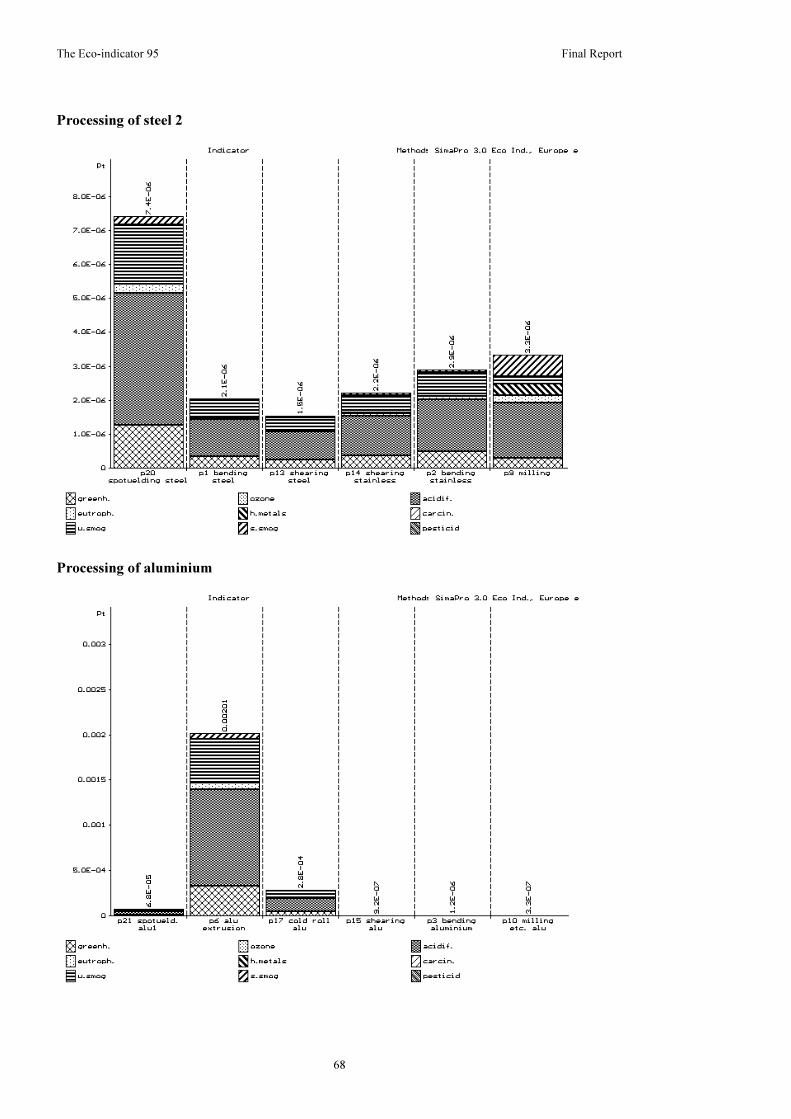
The Eco-indicator 95 Final Report
68
Processing of steel 2
Processing of aluminium

The Eco-indicator 95 Final Report
69
Processing of plastics 1
Processing of plastics 2

The Eco-indicator 95 Final Report
70
Waste treatmentThe graphs show the combined positive and negative effects from waste treatment. The
negative values are subtracted for each effect; the resulting values are plotted in the graph.
Incineration
The negative value for incineration of steel can be explained from the high efficiency of
magnetic separation of scrap in modern incinerators.
Landfill
The values are completely defined by the leaching of heavy metals (modern landfill site)

The Eco-indicator 95 Final Report
71
Recycling
In most cases the avoided emissions are higher than the emissions from the recycling
process. The plastic recycling process is here shown for polyethylene.
Municipal waste

The Eco-indicator 95 Final Report
72
Household waste

The Eco-indicator 95 Final Report
73
Annexe 2: Calculation of normalisation values
The normalisation values are calculated in the large spreadsheet on the following pages. The
structure of the spreadsheet is described below.
The emissions are listed in the top row. Row 2 indicates whether this emission is to air or to
water. Row 3, contains the year of measurement and row 4 and 5 contain information about
the source. The sources are listed below.
Source Title publisher
1 The Environment in Europe and North-America, Annotated Statistics 1992,
Economic Commission for Europe, United Nations Publication [37]
2 Corinair 1990 , provisional results [6]
3 Environmental Statistics 1991, Eurostat, [11]
4 The Environment in Europe: a Global Perspective, RIVM. [33]
5 General Environmental Statistics 1992], CBS (NL), [5]
6 Industrial emissions in the Netherlands No. 14, September 1993, [23]
7 CFC commission, a collaborative project by Government and industry
Annual report 1993, [4]
The countries of Europe are listed twice in column A. In the upper part (row 7 to 33), the
emissions are listed per county, as far as data was available. The sums of the known
emissions are listed in row 26 for Western Europe and in row 34 for Eastern Europe.
In order to calculate the values for the countries with no data, an extrapolation was made
based on the energy consumption per country. The energy consumption was chosen, since it
seems to reflect the infrastructure and industry of a country. Since there are big differences
in industrial structure in Eastern and Western Europe, we have made the extrapolation for
both areas separately.
In cell B38 to B63, the energy use per country is listed. The spreadsheet is programmed in
such a way that, if an emission is known for a certain country, the energy use is copied to
the appropriate column. For instance, The CO2 emission for Germany is known (cell D13),
but the CO2 emission for Greece is not known (cell D14). This means that cell D43 does
contain the German energy consumption, whereas cell D44 remains empty.
Row 56 contains the total energy consumption in counties with known emissions for
Western Europe (Row 64 for Eastern Europe). These figures allow for the calculation of the
average emission per MJ energy use. Multiplication of this figure with the total energy use
provides the extrapolated total emission.
known emission
emission = total energy use x -------------------------------------------------------
energy use in countries with known emissions
The result can be found in row 67 and 68 for Western and Eastern Europe. For a number
emissions there was no data from eastern Europe available at all. In these cases the Eastern
European data was directly extrapolated form Western European data. The result of this
extrapolation can be found in row 69. The final result is listed in row 70, together with the
unit in row 71.
The normalisation values for individual emissions are converted into normalisation values
for effects, using the characterisation values is annexe 3.

The Eco-indicator 95 Final report
74
A B C D E
1 CO2 CH4
2 COMPARTMENT AIR AIR
3 YEAR 1990 1990
4 SOURCE 1 2
5 table I-2.1.6
6 COUNTRY UNIT --> Kilo-Tonnes Kilo-Tonnes
7 EC
8 AUSTRIA 56500
9 BELGIUM 355
10 DENMARK 57900
11 FINLAND 52000
12 FRANCE 279200 3882
13 GERMANY 1070000
14 GREECE
15 ICELAND
16 IRELAND 850
17 ITALY
18 LUXEMBURG
19 THE NETHERLANDS 148000 1040
20 NORWAY 34500 282
21 PORTUGAL 37800 330
22 SPAIN
23 SWEDEN 63000 2106
24 SWITSERLAND 43400
25 UNITED KINGDOM 584800 4288
26 Total known emissions in Western Europe 2427100 13133
27
28 CSSR
29 HUNGARY 87800
30 POLAND 440000 6066
31 ROMANIA 127100
32 BULGARIA
33 EX-YUGOSLAVIA
34 Total known emissions in Eastern Europe 654900 6066
35
36 EXTRAPOLATION ENERGY-USE
37 1988, source 1, table I 1.5.4
38 AUSTRIA 1209.6 PJ 1209.6
39 BELGIUM 1927.8 PJ 1927.8
40 DENMARK 798 PJ 798
41 FINLAND 1239 PJ 1239
42 FRANCE 8773.8 PJ 8773.8 8773.8
43 GERMANY 15573.6 PJ 15573.6
44 GREECE 861 PJ
45 ICELAND 71.4 PJ
46 IRELAND 407.4 PJ 407.4
47 ITALY 6371.4 PJ
48 LUXEMBURG 142.8 PJ
49 THE NETHERLANDS 2709 PJ 2709 2709
50 NORWAY 1176 PJ 1176 1176
51 PORTUGAL 5359.2 PJ 5359.2 5359.2
52 SPAIN 3553.2 PJ
53 SWEDEN 2360.4 PJ 2360.4 2360.4
54 SWITSERLAND 1180.2 PJ 1180.2
55 UNITED KINGDOM 8757 PJ 8757 8757
56 Total energy use of countries with known emissions in Western Europe 62470.8 49135.8 31470.6
57 PJ
58 CSSR 3183.6 PJ
59 HUNGARY 1260 PJ 1260
60 POLAND 5359.2 PJ 5359.2 5359.2
61 ROMANIA 3007.2 PJ 3007.2
62 BULGARIA 1310.4 PJ
63 EX-YUGOSLAVIA 1961.4 PJ
64 Total energy use of countries with known emissions in Eastern Europe 16081.8 PJ 9626.4 5359.2
65
66 RESULTS CO2 CH4
67 Total Western Europe (extrapolated from West Europ. counties) 3.09E+06 2.61E+04
68 Total Eastern Europe (extrapolated from East. Europ. countries) 1.09E+06 1.82E+04
69 Total Eastern Europe (extrapolated from western Eur.)
70 Total emissions East and West Europe 4.18E+06 4.43E+04
71 UNIT --> Kilo-Tonnes Kilo-Tonnes

The Eco-indicator 95 Final report
75
F G H I J K L M N O
1 N2O CFC-11&12 CFC-13 CFC-113 CFC-114 CFC-115 Halon-1211 Halon-1301 CCl4 1,1,1-TCE
2 AIR AIR AIR AIR AIR AIR AIR AIR AIR AIR
3 1990 1990 1990 1990 1990 1990 1990 1990 1990 1990
4 2 3 7 7 7 7 7 7 7 7
5 table pp18 table pp18 table pp18 table pp18 table pp18 table pp18 table pp18 table pp18
6 Kilo-Tonnes Tonnes Tonnes Tonnes Tonnes Tonnes Tonnes Tonnes Tonnes Tonnes
7 209900
8
9 26
10
11
12 210
13
14
15
16 45
17
18
19 25 3 1197 99 105 212 170 777 5540
20 16
21 49
22
23 33
24
25 175
26 579 3 1197 99 105 212 170 777 5540
27
28
29
30 155
31
32
33
34 155
35
36
37
38
39 1927.8
40
41
42 8773.8
43
44
45
46 407.4
47
48
49 2709 2709 2709 2709 2709 2709 2709 2709 2709
50 1176
51 5359.2
52
53 2360.4
54
55 8757
56 31470.6 2709 2709 2709 2709 2709 2709 2709 2709
57
58
59
60 5359.2
61
62
63
64 5359.2
65
66 N2O CFC-11&12 CFC-13 CFC-113 CFC-114 CFC-115 Halon-1211 Halon-1301 CCl4 1,1,1-TCE
67 1.15E+03 2.10E+05 6.92E+01 2.76E+04 2.28E+03 2.42E+03 4.89E+03 3.92E+03 1.79E+04 1.28E+05
68 4.65E+02
69 5.40E+04 1.78E+01 7.11E+03 5.88E+02 6.23E+02 1.26E+03 1.01E+03 4.61E+03 3.29E+04
70 1.61E+03 2.64E+05 8.70E+01 3.47E+04 2.87E+03 3.04E+03 6.15E+03 4.93E+03 2.25E+04 1.61E+05
71 Kilo-Tonnes Tonnes Tonnes Tonnes Tonnes Tonnes Tonnes Tonnes Tonnes Tonnes

The Eco-indicator 95 Final report
76
P Q R S T U V W X
1 HCFK-22 HCFK 141b HCFK 142b CH3Br Total S SO2 NOx NH3 PHOSPHATES
2 AIR AIR AIR AIR AIR AIR AIR AIR AIR
3 1990 1991 1990 1991 1988 1988 1988 1988 1988
4 7 7 7 7 1 1 1 1 1
5 table pp18 table pp18 table pp18 table pp18 table I-2.1.2 table I-2.1.2 table I-2.1.4 table I-2.1.5 table II-3.2.7b
6 Tonnes Tonnes Tonnes Tonnes Kilo-Tonnes Kilo-Tonnes Kilo-Tonnes Kilo-Tonnes Tonnes
7
8 61 121.878 213 81 77528
9 207 413.586 312 94 80300
10 121 241.758 249 125 92000
11 151 301.698 276 140570
12 607 1212.786 1656 841 1459900
13 3270 6533.46 3490 992312
14 112 176420
15 3 5889
16 74 147.852 122 139 160718
17 1205 2407.59 1705 426 715459
18 6 6700
19 2120 25 1023 89 139 277.722 559 254 86257
20 33 65.934 225 41 17376
21 102 203.796 122 55 89100
22 273 462213
23 107 213.786 396 62 68200
24 61 39000
25 1907 3810.186 2642 478 433000
26 2120 25 1023 89 7984 15952.032 11967 3051 5102942
27
28 1402 2801.196 965 200 460092
29 609 1216.782 259 151 347216
30 2067 4129.866 1551 55 943708
31 2400 4795.2 21 9 329296
32 1562 3120.876 388 10 258152
33 800 1598.4 480 61 261408
34 8840 17662.32 3664 486 2599872
35
36
37
38 1209.6 1209.6 1209.6 1209.6 1209.6
39 1927.8 1927.8 1927.8 1927.8 1927.8
40 798 798 798 798 798
41 1239 1239 1239 1239
42 8773.8 8773.8 8773.8 8773.8 8773.8
43 15573.6 15573.6 15573.6 15573.6
44 861 861
45 71.4 71.4
46 407.4 407.4 407.4 407.4 407.4
47 6371.4 6371.4 6371.4 6371.4 6371.4
48 142.8 142.8
49 2709 2709 2709 2709 2709 2709 2709 2709 2709
50 1176 1176 1176 1176 1176
51 5359.2 5359.2 5359.2 5359.2 5359.2
52 3553.2 3553.2
53 2360.4 2360.4 2360.4 2360.4 2360.4
54 1180.2 1180.2
55 8757 8757 8757 8757 8757
56 2709 2709 2709 2709 56662.2 56662.2 56662.2 45658.2 62470.8
57
58 3183.6 3183.6 3183.6 3183.6 3183.6
59 1260 1260 1260 1260 1260
60 5359.2 5359.2 5359.2 5359.2 5359.2
61 3007.2 3007.2 3007.2 3007.2 3007.2
62 1310.4 1310.4 1310.4 1310.4 1310.4
63 1961.4 1961.4 1961.4 1961.4 1961.4
64 16081.8 16081.8 16081.8 16081.8 16081.8
65
66 HCFK-22 HCFK 141b HCFK 142b CH3Br Total S SO2 NOx NH3 PHOSPHATES
67 4.89E+04 5.77E+02 2.36E+04 2.05E+03 8.80E+03 1.76E+04 1.32E+04 4.17E+03 5.10E+06
68 8.84E+03 1.77E+04 3.66E+03 4.86E+02 2.60E+06
69 1.26E+04 1.48E+02 6.07E+03 5.28E+02
70 6.15E+04 7.25E+02 2.97E+04 2.58E+03 1.76E+04 3.52E+04 1.69E+04 4.66E+03 7.70E+06
71 Tonnes Tonnes Tonnes Tonnes Kilo-Tonnes Kilo-Tonnes Kilo-Tonnes Kilo-Tonnes Tonnes

The Eco-indicator 95 Final report
77
Y Z AA AB AC AD AE AF AG
1 NITRATES NMVOC VOC SPM Disinfectants Fungicides Herbicides Insecticides Cd
2 AIR AIR AIR AIR WATER WATER WATER WATER AIR
3 1988 1990 1988 1988 1990 1990 1990 1990 1990
4 1 2 1 1 4 4 4 4 5
5 table II-3.2.7b table I-2.1.6 table I-2.1.5 table 8.01
6 Tonnes Kilo-Tonnes Kilo-Tonnes Kilo-Tonnes Tonnes Tonnes Tonnes Tonnes Tonnes
7
8 139550 466 39
9 180600 386 900 2160 4770 306
10 377000 76 1555 4506 289
11 1994499
12 2603700 2856 284 4807 49775 36075 6657
13 2413118 3150 2730 10151 14756 4558
14 409216 640 10384 3411 2818
15 11454
16 349025 197 136
17 924912 827 452 27934 9234 2941
18 16400
19 455650 460 487 93 9830 4063 3271 1554 2.4
20 110100 270 248 21
21 665240 649 156 21288 1055 587
22 976023 4518 33496 6360 2643
23 209700 722 460
24 71500 22
25 1462000 2690 2013 533 76 5522 19625 690
26 13369687 8230 7943 4174 20847 166328 103063 23043 2.4
27
28 636207 313 1245
29 650943
30 1520618 1411 1000 1615
31 662400 785
32 427495 24 808
33 502984
34 4400647 1411 1337 4453
35
36
37
38 1209.6 1209.6 1209.6
39 1927.8 1927.8 1927.8 1927.8 1927.8 1927.8
40 798 798 798 798 798
41 1239
42 8773.8 8773.8 8773.8 8773.8 8773.8 8773.8 8773.8
43 15573.6 15573.6 15573.6 15573.6 15573.6 15573.6
44 861 861 861 861 861
45 71.4
46 407.4 407.4 407.4
47 6371.4 6371.4 6371.4 6371.4 6371.4 6371.4
48 142.8
49 2709 2709 2709 2709 2709 2709 2709 2709 2709
50 1176 1176 1176 1176
51 5359.2 5359.2 5359.2 5359.2 5359.2 5359.2
52 3553.2 3553.2 3553.2 3553.2 3553.2
53 2360.4 2360.4 2360.4
54 1180.2 1180.2
55 8757 8757 8757 8757 8757 8757 8757 8757
56 62470.8 31470.6 43923.6 45750.6 27379.8 54684 54684 54684 2709
57
58 3183.6 3183.6 3183.6
59 1260
60 5359.2 5359.2 5359.2 5359.2
61 3007.2 3007.2
62 1310.4 1310.4 1310.4
63 1961.4
64 16081.8 5359.2 9853.2 12860.4
65
66 NITRATES NMVOC VOC SPM Disinfectants Fungicides Herbicides Insecticides Cd
67 1.34E+07 1.63E+04 1.13E+04 5.70E+03 4.76E+04 1.90E+05 1.18E+05 2.63E+04 5.53E+01
68 4.40E+06 4.23E+03 2.18E+03 5.57E+03
69 1.22E+04 4.89E+04 3.03E+04 6.78E+03 1.42E+01
70 1.78E+07 2.06E+04 1.35E+04 1.13E+04 5.98E+04 2.39E+05 1.48E+05 3.31E+04 6.96E+01
71 Tonnes Kilo-Tonnes Kilo-Tonnes Kilo-Tonnes Tonnes Tonnes Tonnes Tonnes Tonnes

The Eco-indicator 95 Final report
78
AH AI AJ AK AL AM AN AO AP AQ AR
1 Pb Mn Hg C6H6 PAH Sb As Ba B Cd Cr(III&VI)
2 AIR AIR AIR AIR AIR WATER AIR WATER WATER WATER WATER
3 1988 1990 1990 1990 1990 1990 1987 1990 1990 1990 1990
4 1 6 6 6 6 6 5 6 6 6 6
5 table I-2.1.6 table 4.1a table 4.1a table 4.1a table 4.1a table 4.2 table 8.03 table 4.2 table 4.2 table 4.2 table 4.2
6 Kilo-Tonnes Tonnes Tonnes Tonnes Tonnes Tonnes Tonnes Tonnes Tonnes Tonnes Tonnes
7
8 0.258
9
10
11 0.45
12
13 3
14
15
16
17
18
19 0.45 22.38 2.82 737.54 183.58 0.64 1.3 1.03 31.4 3.98 16.07
20 0.28
21
22
23
24
25 3.1
26 7.538 22.38 2.82 737.54 183.58 0.64 1.3 1.03 31.4 3.98 16.07
27
28
29
30 1.6
31 0.8
32 0.2
33
34 2.6
35
36
37
38 1209.6
39
40
41 1239
42
43 15573.6
44
45
46
47
48
49 2709 2709 2709 2709 2709 2709 2709 2709 2709 2709 2709
50 1176
51
52
53
54
55 8757
56 30664.2 2709 2709 2709 2709 2709 2709 2709 2709 2709 2709
57
58
59
60 5359.2
61 3007.2
62 1310.4
63
64 9676.8
65
66 Pb Mn Hg C6H6 PAH Sb As Ba B Cd Cr(III&VI)
67 1.54E+01 5.16E+02 6.50E+01 1.70E+04 4.23E+03 1.48E+01 3.00E+01 2.38E+01 7.24E+02 9.18E+01 3.71E+02
68 4.32E+00
69 1.33E+02 1.67E+01 4.38E+03 1.09E+03 3.80E+00 7.72E+00 6.11E+00 1.86E+02 2.36E+01 9.54E+01
70 1.97E+01 6.49E+02 8.18E+01 2.14E+04 5.32E+03 1.86E+01 3.77E+01 2.99E+01 9.11E+02 1.15E+02 4.66E+02
71 Kilo-Tonnes Tonnes Tonnes Tonnes Tonnes Tonnes Tonnes Tonnes Tonnes Tonnes Tonnes

The Eco-indicator 95 Final report
79
AS AT AU AV AW AX AY AZ BA BB
1 Cu Pb Mn Hg Mo Ni Ni As ENERGY-USE WASTE
2 WATER WATER WATER WATER WATER WATER AIR WATER
3 1990 1990 1990 1990 1990 1990 1990 1987 1988 1988
4 6 6 6 6 6 6 6 5 1 1
5 table 4.2 table 4.2 table 4.2 table 4.2 table 4.2 table 4.2 table 4.1a table 8.0.3 table I-1.5.4 table I-2.3.3
6 Tonnes Tonnes Tonnes Tonnes Tonnes Tonnes Tonnes Tonnes TJ Kilo tonnes
7
8 1209.6 2449
9 1927.8 900
10 798
11 1239 1285
12 8773.8 15500
13 15573.6 31623
14 861
15 71.4 93
16 407.4 1270
17 6371.4 17300
18 142.8 170
19 17.23 17.24 500.9 0.39 2.14 20.01 4.26 56.2 2709 6500
20 1176 2000
21 5359.2 2678
22 3553.2 10600
23 2360.4 2650
24 1180.2 2850
25 8757 20000
26 17.23 17.24 500.9 0.39 2.14 20.01 4.26 56.2 62470.8 117868
27
28 3183.6 872.2
29 1260 7000
30 5359.2 46418
31 3007.2
32 1310.4
33 1961.4
34 16081.8 54290.2
35
36
37
38 1209.6 1209.6
39 1927.8 1927.8
40 798
41 1239 1239
42 8773.8 8773.8
43 15573.6 15573.6
44 861
45 71.4 71.4
46 407.4 407.4
47 6371.4 6371.4
48 142.8 142.8
49 2709 2709 2709 2709 2709 2709 2709 2709 2709 2709
50 1176 1176
51 5359.2 5359.2
52 3553.2 3553.2
53 2360.4 2360.4
54 1180.2 1180.2
55 8757 8757
56 2709 2709 2709 2709 2709 2709 2709 2709 62470.8 60811.8
57
58 3183.6 3183.6
59 1260 1260
60 5359.2 5359.2
61 3007.2
62 1310.4
63 1961.4
64 16081.8 9802.8
65
66 Cu Pb Mn Hg Mo Ni Ni As ENERGY-USE WASTE
67 3.97E+02 3.98E+02 1.16E+04 8.99E+00 4.93E+01 4.61E+02 9.82E+01 1.30E+03 6.25E+04 1.21E+05
68 1.61E+04 8.91E+04
69 1.02E+02 1.02E+02 2.97E+03 2.32E+00 1.27E+01 1.19E+02 2.53E+01 3.34E+02
70 5.00E+02 5.00E+02 1.45E+04 1.13E+01 6.21E+01 5.80E+02 1.24E+02 1.63E+03 7.86E+04 2.10E+05
71 Tonnes Tonnes Tonnes Tonnes Tonnes Tonnes Tonnes Tonnes TJ Kilo tonnes

The Eco-indicator 95 Final report
80
Annexe 3: Characterisation values
This annexe contains the characterisation values, that are used in the calculation of the
indicator values and the normalisation values.
Cat. Substance Weight factor Unit
Class: greenhouse effect, Unit GWP
Air 1,1,1-trichloroethane 100 kgAir CFC (hard) 7100 kgAir CFC (soft) 1600 kgAir CFC-11 3400 kgAir CFC-113 4500 kgAir CFC-114 7000 kgAir CFC-115 7000 kgAir CFC-12 7100 kgAir CFC-13 13000 kgAir CO2 1 kgAir dichloromethane 15 kgAir HALON-1211 4900 kgAir HALON-1301 4900 kgAir HCFC-123 90 kgAir HCFC-124 440 kgAir HCFC-141b 580 kgAir HCFC-142b 1800 kgAir HCFC-22 1600 kgAir HFC-125 3400 kgAir HFC-134a 1200 kgAir HFC-143a 3800 kgAir HFC-152a 150 kgAir methane 11 kgAir N2O 270 kgAir tetrachloromethane 1300 kgAir trichloromethane 25 kg
Class: ozone depletion. Unit: ODP
Air 1,1,1-trichloroethane 0.12 kgAir CFC (hard) 1 kgAir CFC (soft) 0.055 kgAir CFC-11 1 kgAir CFC-113 1.07 kgAir CFC-114 0.8 kgAir CFC-115 0.5 kgAir CFC-12 1 kgAir CFC-13 1 kgAir HALON-1201 1.4 kgAir HALON-1202 1.25 kgAir HALON-1211 4 kgAir HALON-1301 16 kgAir HALON-2311 0.14 kgAir HALON-2401 0.25 kgAir HALON-2402 7 kgAir HCFC-123 0.02 kgAir HCFC-124 0.022 kgAir HCFC-141b 0.11 kgAir HCFC-142b 0.065 kgAir HCFC-22 0.055 kgAir HCFC-225ca 0.025 kgAir HCFC-225cb 0.033 kgAir methyl bromide 0.6 kg

The Eco-indicator 95 Final report
81
Air tetrachloromethane 1.08 kg
Class: acidification, Unit: AP
Air ammonia 1.88 kgAir HCl 0.88 kgAir HF 1.6 kgAir NO 1.07 kgAir NO2 0.7 kgAir NOx 0.7 kgAir SO2 1 kgAir SOx 1 kg
Class: Nutriphication, Unit: NP
Air ammonia 0.33 kgAir nitrates 0.42 kgAir NO 0.2 kgAir NO2 0.13 kgAir NOx 0.13 kgAir phosphate 1 kgWater COD 0.022 kgWater NH3 0.33 kgWater NH4+ 0.33 kgWater Ntot 0.42 kgWater phosphate 1 kgWater Ptot 3.06 kg
Class: heavy metals, Unit: Pb equivalent
Air cadmium oxyde 50 kgAir Cd 50 kgAir heavy metals 1 kgAir Hg 1 kgAir Mn 1 kgAir Pb 1 kgWater As 1 kgWater B 0.03 kgWater Ba 0.14 kgWater Cd 3 kgWater Cr 0.2 kgWater Cu 0.005 kgWater Hg 10 kgWater Mn 0.02 kgWater Mo 0.14 kgWater Ni 0.5 kgWater Pb 1 kgWater Sb 2 kg
Class: carcinogenesis, Unit: PAH equivalent
Air As 0.044 kgAir benzene 0.000011 kgAir benzo[a]pyrene 1 kgAir Cr (6+) 0.44 kgAir CxHy aromatic 0.000011 kgAir ethylbenzene 0.000011 kgAir fluoranthene 1 kgAir Ni 0.44 kgAir PAH 1 kgAir tar 0.000011 kg

The Eco-indicator 95 Final report
82
Class: winter smog, Unit: SO2 equivalent
Air dust (SPM) 1 kgAir SO2 1 kgAir Soot 1 kg
Class: summer smog, Unit: PCOP
Air 1,1,1-trichloroethane 0.021 kgAir 1,2-dichloroethane 0.021 kgAir acetone 0.178 kgAir acetylene 0.168 kgAir alcohols 0.196 kgAir aldehydes 0.443 kgAir benzene 0.189 kgAir caprolactam 0.761 kgAir chlorophenols 0.761 kgAir crude oil 0.398 kgAir CxHy 0.398 kgAir CxHy aliphatic 0.398 kgAir CxHy aromatic 0.761 kgAir CxHy chloro 0.021 kgAir dichloromethane 0.021 kgAir diethyl ether 0.398 kgAir diphenyl 0.761 kgAir ethanol 0.268 kgAir ethene 1 kgAir ethylene glycol 0.196 kgAir ethylene oxide 0.377 kgAir formaldehyde 0.421 kgAir hexachlorobiphenyl 0.761 kgAir hydroxy compounds 0.377 kgAir isopropanol 0.196 kgAir ketones 0.326 kgAir methane 0.007 kgAir methyl ethyl ketone 0.473 kgAir methyl mercaptane 0.377 kgAir naphthalene 0.761 kgAir non methane VOC 0.416 kgAir PAH 0.761 kgAir pentane 0.408 kgAir petrol 0.398 kgAir phenol 0.761 kgAir phthalic acid anhydride 0.761 kgAir propane 0.42 kgAir propene 1.03 kgAir propionaldehyde (propanal) 0.603 kgAir styrene 0.761 kgAir terpentine 0.377 kgAir tetrachloromethane 0.021 kgAir toluene 0.563 kgAir trichloroethene 0.066 kgAir vinylacetate 0.223 kgAir vinylchloride 0.021 kgAir VOC 0.398 kgAir xylene 0.85 kg
Class: pesticides Unit: Active substance
Water desinfectants 1 kgWater fungicides 1 kgWater herbicides 1 kgWater insecticides 1 kg

The Eco-indicator 95 Final report
83
Annexe 4: Data sources for inventories.
The annexe report 9510A contains a full specification of the impact tables used to calculate the Eco-indicators. Since this version is only available in Dutch, we included a short list with data references inthis report. The following tables contain a code in the second column representing the data sourceused. The third column contains some additional specification or a source that is only used once ortwice. Sources printed in italics refer to commercial companies. The codes used in the second columnshould be read as:B Habesatter et al. Oekobilanz von Packstoffen Stand 1990 [Environmental audit of packaging
materials, as at 1990], ETH Zurich, Buwal publication 132, 1991, Bern, Switzerland.bj Bergh en Jurgens, Milieueffecten van Verpakkingsmaterialen [Environmental Impacts of
Packaging Materials]; Rotterdam; August 1990E Frischknecht, R.; Hofstetter, P.; Knoepfel, I.; Ökoinventare für Energy Systeme [Environmental
inventories for energy systems]; ETH Zurich, March 1994.S SPIN project: a series of publications. The authors are indicated in the tables below. Information:
RIVM LAE, Bilthoven, The Netherlands.v H van Heijningen, R.J.J.; Castro de, J.F.M.; Meer energiekentallen in relatie tot preventie en
hergebruik van afvalstromen; NOH 1992HE Reijnders, Handbook of emission factors, Government Publishing house, The Hague 1993K Kemna, R.B.J.; Energiebewust ontwerpen, TU Delft, 1981, herdruk 1992P PWMI, Ecoprofiles on the European Plastics Industry, PWMI 1993-95
Production of metalsSource Specification
Secondary aluminium bj
Aluminium B
Copper, primary E
Copper, 60% primary interpolationSecondary copper E
Other non-ferrous metals estimateStainless steel S+E + World resources [40]+ Metals and Minerals 1992Secondary steel B
Steel B
Sheet steel B
Processing of steelSource Specification
Bending steel K+S Spin: Roos, B; Metaalbewerking; RIVMBending stainless steel K+S Spin: Roos, B; Metaalbewerking; RIVMCutting steel K
Cutting stainless steel K
Pressing and deep-drawing K
Rolling (cold) K+S Spin: Huizinga, K.; Non ferro walserijen; RIVM; 1992Spot-welding K
Machining K
Machining (per volume) CalculatedHot-galvanising S Meijer, R.P.B.; Thermisch verzinken; RIVM; 1992Electrolytic galvanising K + Mortier, J.W.; Galvanische processen, 1992Electroplating (chrome) K + Mortier, J.W.; Galvanische processen, 1992

The Eco-indicator 95 Final report
84
Processing of aluminium
Source Specification
Blanking and cutting K
Bending K+S Spin: Roos, B; Metaalbewerking; RIVMRolling (cold) K+S Spin: Huizinga, K.; Non ferro walserijen; RIVM; 1992Spot-welding K
Machining K
Machining (per volume) CalculatedExtrusion K
Production of plastic granulate
Source Specification
ABS vH+HE
HDPE P
LDPE P
Natural rubber based on "Emmissie registratie" compiled byRemmerswaal; TU Delft
PA bj
PC no source extrapolated using the energy requirements as basisPET P
PP P
PPE/PS based on "Emissieregistratie", compiled by Remmerswaal;TU Delft
PS rigid foam P
PS high impact (HIPS) P
PUR E + Chemiewinkel, University of Amsterdam, 1994PVC P
Processing of plastics
Source Specification
Injection mould. in general Mulder, S; Energiebesparing spuitgietmachines; Kunststofen Rubber 9; 1994
Inject. mould. PVC & PC Mulder, S; Energiebesparing spuitgietmachines; Kunststofen Rubber 9; 1994
RIM, PUR Recticel
Extrusion blowing PE internal Procter and Gamble LCI spreadsheet, 1994
Vacuum forming Nelipak Venray B.V.
Vacuum pressure forming Nelipak Venray B.V.
Calandering of PVC K
Foil blowing PE internal Procter and Gamble LCI spreadsheet, 1994
Ultrasonic welding Philips CFT
Machining K
Production of other materials
Source Specification
Glass B
Glass wool and glass fibre S Loos; De productie van glas en glaswol; RIVM; April1992.
Rockwool S Kaskens, H.J.M et al; Produktie van steenwol; RIVM;Januari 1992
Ceramics S Huizinga, K; Fijnkeramische industrie; RIVM; July 1992Cellulose board B
Paper B
Recycled paper B
Wood H. Boorsma; Houtvademecum; Centrum Hout; Almere1990
Cardboard B

The Eco-indicator 95 Final report
85
Production of energy
Source Description
Electricity high voltage E
Electricity low voltage E
Heat from gas (MJ) B
Heat from oil (MJ) B
Mechanical (diesel, MJ) B
Transport
Source Specification
Truck (28 ton) E
Truck (75m3) calculatedTrain E
Container ship E
Aircraft Emissieregistratie 1990, compiled by Remmerswaal; TUDelft; + Fuel consumption and emissions of air traffic1990; Olivier, J.;Inventory of Aircraft emissions; RIVM1991.
Waste processing and recycling
Source Specification
All data on waste taken form SimaPro 3.0; based on data from the AOO[Waste Consulting Body in the Netherlands]