The e�ects of rural/urban movement on Dengue

transmission dynamics

Alejandra Gaitan1, Jasmine Jackson2, Olivia Justynski3, Danielle Williams4.

I Made Eka Dwipayana5, Komi Messan5, Omayra Ortega5, Fabio Sanchez6,5

1Universidad de Colima, Colima, Mexico2Norfolk State University, Norfolk, VA

3Mount Holyoke College, South Hadley, MA4East Stroudsburg University, East Stroudsburg, PA

5Arizona State University, Tempe, AZ6Universidad de Costa Rica, San Pedro Montes de Oca, San José, Costa Rica

July 25, 2014

Abstract

Five serotypes of Dengue (DENV1-DENV5), a vector-borne disease transmitted bytwo species of mosquitoes, Aedes aegypti and Aedes albopictus, are prevalent in varioustropical and subtropical regions of the world, posing a serious health threat to humans.Dengue is no longer restricted to tropical regions due to increasing levels of mobilityvia travel, migration, or displacement due to con�ict. We use a system of nonlinear or-dinary di�erential equations to explore the e�ects of rural/urban movement on Denguetransmission dynamics. The model incorporates movement between rural and urbanregions. The population of hosts is subdivided into susceptible, exposed, infectious,and recovered classes. Vectors, assumed to remain in a single region, are divided intorural (Ae. albopictus) and urban (Ae. aegypti) populations. The vector populationsare subdivided into susceptible, exposed, and infectious classes. We compute the basicreproductive number (R0) for the system with and without movement and use thiskey dimensionless parameter to study the e�ects of rural/urban host movement onDengue dynamics.

1

1 Introduction

Dengue fever is a mosquito-borne viral infection that is endemic in tropical regions world-wide and may be periodically epidemic in subtropical or temperate regions [11]. It occursin over 100 countries, putting over 2.5 billion people at risk of infection, though it is mostcommon in Central America and Southeast Asia [3, 5]. Classical Dengue Fever (CDF),the most common form of the disease, usually occurs in people over 15 years of age [13].Its symptoms can include fever, headache, nausea, and vomiting with a duration of 3-7days [13]. CDF is usually mild or even asymptomatic [24].

The more severe case, Dengue Hemorrhagic Fever (DHF), usually occurs in childrenunder 15 years of age (though it may be observed in adults). DHF is associated withDengue Shock Syndrome (DSS), and can lead to circulatory failure and death [13,24]. Thefactors that cause Dengue patients to contract DHF and DSS are not fully understood;however, current hypotheses suggest that this more severe form occurs in patients whohave previously recovered from a di�erent serotype of Dengue [11]. DHF and DSS tend toa�ect two categories of Dengue patients: those who are experiencing a secondary infectionand infants whose mothers were previously infected by Dengue [13].

It is estimated that 50-100 million people contract Dengue yearly, while 250,000-500,000people su�er from DHF [29]. There are approximately 22,000 deaths annually, mostlyamong young children [3].

Dengue is caused by �ve antigenically distinguishable serotypes (DENV1 - DENV5) ofthe genus Flavivirus [3,16,24]. Once an individual has been infected by one serotype, theyare permanently immune to that serotype but only temporarily immune to the others [13].The �fth serotype was very recently discovered, and is the only new serotype found in thelast �fty years. Its discovery has made e�orts to control and vaccinate for Dengue evenmore di�cult [22].

There is not yet any speci�c treatment or e�ective vaccine for Dengue, though in somecases, �uid replacement therapy may be used [3, 16]. Several candidates for a Denguevaccine have been clinically tested, but no vaccine has yet been applied on a broad scale[9, 29]. It is speculated that no vaccine could completely protect against all serotypesof the disease [16]. Currently, the main focus is on prevention by controlling mosquitopopulations and breeding sites [3].

DENV is transmitted by two species of mosquitoes: Aedes aegypti and Aedes albopictus.Ae. aegypti is the principal vector of Dengue viruses and has adapted to live closely withhumans. This has made Ae. aegypti one of the most e�cient mosquitoes for transmittingarboviruses, as they feed primarily on humans for blood meals, mostly during the day orin shaded areas at night [23]. These mosquitoes are highly resilient in both the adult andjuvenile stages; their eggs can survive without water for up to six months [15]. They arecommon in urban areas, where they live close to houses and use water-holding containers,preferably in dark colors, for their reproduction. Their bite is often painless and they movequickly, though they do not �y very far [32].

Ae. albopictus, also called the Asian Tiger mosquito, is even more dangerous to humans

2

and domesticated animals. In addition to feeding on humans for blood meals, it will alsofeed on dogs, cats, squirrels, and deer. They are very aggressive all day long and have arapid bite [32]. They prefer to use natural locations, such as plants, to lay their eggs [30].They transmit not only the Dengue virus, but other vector-borne diseases such as WestNile, Eastern equine encephalitis, and Japanese encephalitis viruses as well [14, 30].

Demographics, social change, infrastructure, and other factors related to urbanizationcontribute to the spread of dengue to new populations of mosquitoes [27]. Dengue emergesin tropical and subtropical areas as they are urbanized [31]. The extreme population growththat accompanies urbanization causes overcrowding, poor sanitation, and an increased needfor water storage. This environment encourages the breeding of Ae. aegypti (which thrivein urban areas). Thus, the potential of DENV to spread from city to city via humandisplacement is increased [12,31]. These factors have contributed to the rapid evolution ofDENV, causing a serious public health problem [19].

2 Mathematical model

We explore the dynamics of Dengue fever among humans and female mosquitoes of thespecies Ae. aegypti and Ae. albopictus. The model is divided into rural and urban pop-ulations, between which only host movement can occur. These populations are furthersubdivided into susceptible, exposed, infectious, and recovered classes. The system is com-partmentally symmetric, so the principles and patterns for the rural population also applyto the urban population, and vice versa. However, there are di�erences between someparameter values due to the di�erent species of vectors, which, although they transmit thesame disease, have di�erent capabilities.

Table 1: State variablesState Variable Description

SHR Population of susceptible hosts in a rural area

EHR Population of exposed hosts in a rural area

IHR Population of infectious hosts in a rural area

RHR Population of recovered hosts in a rural area

SHU Population of susceptible hosts in an urban area

EHU Population of exposed hosts in an urban area

IHU Population of infectious hosts in an urban area

RHU Population of recovered hosts in an urban area

SV R Population of susceptible vectors in a rural area

EV R Population of exposed vectors in a rural area

IV R Population of infectious vectors in a rural area

SV U Population of susceptible vectors in an urban area

EV U Population of exposed vectors in an urban area

IV U Population of infectious vectors in an urban area

3

Figure 1: Transmission dynamics for rural (R) and urban (U) host populations.

The total host (H) population, NH , is constant, while the host subpopulations, NHR

and NHU , are not constant when movement occurs. The vector (V ) subpopulations, NV R

and NV U , are constant. We assume that vectors do not move between populations, due totheir limited �ight range.

The susceptible classes, SHR and SHU , are increased by a constant birth rate µHNH

and a factor of movement fR(I ,N )SHR or fU (I ,N )SHU . This class is decreased byindividuals who die of natural causes or move away, and individuals who become exposedat the constant rates βR and βU , which describe the transmission rates of DENV from theproportion of infectious vectors ( IV RNV R

and IV UNV U

) to susceptible hosts.Once a susceptible host is bitten by an infectious vector, they may become exposed to

Dengue. The rates of transmission of Dengue from infectious vectors to susceptible hostsdi�er between rural and urban areas because the Ae. albopictus, which is found in ruralareas, and Ae. aegypti, which is found in urban areas, have di�erent biological propertiesthat a�ect the overall rate of Dengue transmission. The exposed classes, EHR and EHU ,

4

consist of individuals who are in the latency period as a result of DENV infection. Indi-viduals in these classes cannot infect susceptible vectors. Research suggests that latencyperiods last between three to �ve days [21]. While in the exposed classes, individuals areasymptomatic and are not aware that they have the virus, so they are assumed to moveas if they were uninfected. The exiting rate α is de�ned as the rate at which individualscomplete the incubation period, become infectious, and begin to experience symptoms.

Individuals in the infectious classes, IHR and IHU , can transmit the disease to suscep-tible vectors. Once an individual progresses to the infectious class, their rate of movementmay be a�ected by the symptoms they experience, so the movement rates, γR(I ,N ) andγU (I ,N ), is proportional to the movement rates of the uninfectious classes. We assumethat some proportion p ∈ [0, 1], of the infectious individuals remain mobile enough to movenormally, while (1− p) are too ill to move as they ordinarily would. The infectious periodof Dengue fever lasts an average of six days before individuals enter the recovered classes,RHR and RHU , at the recovery rate δ [10].

The recovered classes consist of individuals who are permanently immune to the par-ticular serotype of Dengue. Since they can neither infect nor be infected by vectors, therural/urban movement between these classes is omitted from the model for the sake ofsimplicity.

Figure 2: Transmission dynamics for rural and urban vector populations.

The vector's subpopulations are compartmentally symmetric, as patterns and ideashold true for both the urban and rural species, though the experimentally determinedvalues of these parameters di�er between the species. µV R and µV U are the rates at which

5

vectors mature into adults, become susceptible to DENV, and enter the classes SV R andSV U , respectively. The rates of entry into the exposed classes, EV R and EV U , are φR andφU , respectively. These are the transmission rates as a susceptible vector bites an infectioushost, so this rate also depends on the proportion of infectious hosts ( IHRNHR

and IHUNHU

). Weassume that only the proportion p of infectious hosts who are mobile are available to bebitten by the vectors. That is, the proportion (1 − p) of infectious hosts who are too illto be mobile will be isolated, bedridden, or hospitalized, and vectors will be unable tobite them. After the blood meal from an infectious host is consumed, the vector enters alatency stage, in which they are exposed to DENV but cannot transmit the disease. Theexposed classes are decreased by natural death and progression (at rates θR and θU ) to theinfectious classes, IV R and IV U . Extrinsic incubation lasts ten days, on average, before thevector becomes infectious. Since the vector's lifespan is approximately two to three weeks,it is important to consider the exposed class because some mosquitoes will die before theycan progress to the infectious class. Due to their relatively short lifespan, vectors remaininfectious for life and never recover.

The system of nonlinear ordinary di�erential equations for our model is given by

S′HR = µHNHR − βRIV RNV R

SHR − fR(I ,N )SHR + fU (I ,N )SHU − µHSHR,

E′HR = βRIV RNV R

SHR − αEHR − fR(I ,N )EHR + fU (I ,N )EHU − µHEHR,

I ′HR = αEHR − δIHR − γR(I ,N )IHR + γU (I ,N )IHU − µHIHR,R′HR = δIHR − µHRHR,

S′HU = µHNHU − βUIV UNV U

SHU + fR(I ,N )SHR − fU (I ,N )SHU − µHSHU ,

E′HU = βUIV UNV U

SHU − αEHU + fR(I ,N )EHR − fU (I ,N )EHU − µHEHU ,

I ′HU = αEHU − δIHU + γR(I ,N )IHR − γU (I ,N )IHU − µHIHU , (1)

R′HU = δIHU − µHRHU ,

6

S′V R = µV RNV R − φRpIHRNHR

SV R − µV RSV R, (2)

E′V R = φRpIHRNHR

SV R − θREV R − µV REV R,

I ′V R = θREV R − µV RIV R,

S′V U = µV UNV U − φUpIHUNHU

SV U − µV USV U ,

E′V U = φUpIHUNHU

SV U − θUEV U − µV UEV U ,

I ′V U = θUEV U − µV UIV U ,where

NHR = SHR + EHR + IHR +RHR, (3)

NHU = SHU + EHU + IHU +RHU ,

NV R = SV R + EV R + IV R,

NV U = SV U + EV U + IV U .

With this model, our main goal is to analyze the e�ect of human movement on thetransmission dynamics of Dengue. For the sake of comparison, we �rst analyze the systemfor a case in which there is no movement between the rural and urban areas.

In this case, we analyze the complete system as two independent systems where therural population is a�ected by Ae. albopictus and the urban population is a�ected by Ae.

aegypti. These particular vectors are selected for these areas because they are observed toprefer those respective habitats. Since these two models are compartmentally symmetric,we �rst analyze the zero-movement model as consisting of only one host population andone vector population, each with a constant population.

In the second case we consider constant movement. In this model, we consider di�erentscenarios for the rural and urban populations due to the fact that the species of vectorsthat are native to each area have di�erent qualities. We assume that the urban and ruralhost populations are not constant (due to movement between them), but that the totalhost population is constant. We de�ne movement rates as a constant that designates thebase rate of movement. In this case, the movement rates between the susceptible classesare equal to the movement rates between the exposed classes, since an exposed individualis asymptomiatic and will not show a change in behavior. However, the movement ratesbetween the infectious classes are a reduced rate. We assume that some proportion (1− p)of the infectious population is too ill to move normally, and so they are removed from themovement rates. We assume that the same constant p applies in both the rural and urbanpopulations, as the severity of illness will not change with respect to location.

The �nal case introduces non-constant functions to describe the movement rates. Thesefunctions are de�ned as fR(I ,N ) and fU (I ,N ), where fR is the rate of rural to ur-ban movement, fU is the rate of urban to rural movement, I = (IHR, IHU ), and N =

7

(NHR, NHU ). We consider the change in movement rate to depend on the relative propor-tions of infectious populations. We assume that when there are no infectious hosts, themovement rates are equal to the constant movement rates CR and CU , while the presenceof infectious individuals will modify these base rates. We assume that when there is anincreased proportion of infectious hosts in the rural area, movement towards the rural areais less likely and movement away from the rural area is more likely; the equivalent is truefor an increased proportion of infectious hosts in the urban area. We analyze functionsthat modify the base movement rates and describe the rates in terms of the proportionsof infectious hosts to the total population in each area. We use this proportion, ratherthan the raw number of infectious individuals, because the rural and urban populationsare likely to be very di�erent in total size.

3 Descriptions and Values for Variables and Parameters

The following parameter values are based on experimental data from previous researchwhere referenced.

Table 2: ParametersParameter Description Units

µH Host natural mortality rate Time−1

µV R Vector mortality rate in rural areas Time−1

µV U Vector mortality rate in urban areas Time−1

βR Transmission rate for rural hosts Time−1

βU Transmission rate for urban hosts Time−1

φR Transmission rate for rural vectors Time−1

φU Transmission rate for urban vectors Time−1

α Rate of advancement from exposed to infectious hosts Time−1

θR Rate of advancement from rural exposed to infectious vectors Time−1

θU Rate of advancement from urban exposed to infectious vectors Time−1

δ Host recovery rate Time−1

CR Rate of rural → urban movement in disease-free case Time−1

CU Rate of urban → rural movement in disease-free case Time−1

p Proportion of infectious hosts that are mobile Dimensionless

8

Table 3: Parameter valuesParameter Mean Minimum Maximum Reference

µH1/75∗365 days [7]

µV R 1/21 1/42 1/14 [2, 6, 20]

µV U 1/14 1/42 1/8 [8, 18, 26]

α 1/5 1/7 1/4 [17, 25]

θR 1/10 1/14 1/7 [2]

θU 1/10 1/14 1/7 [4, 17]

δ 1/6 1/12 1/4 [1, 10]

p 0.9 0 1

CR 0.42 0 1

CU 0.24 0 1

4 Mathematical Analysis

4.1 Zero Movement

4.1.1 System Equations

In the �rst and most simple case, we examine the system without movement, that is, where

fR(I ,N ) = fU (I ,N ) = 0.

No movement between rural and urban populations implies the existence of two inde-pendent compartmentally symmetric systems. This allows us to analyze a model for thetransmission of Dengue in a single area and with a particular kind of mosquito.

We denote by NH and NV the total host and vector population sizes, respectively, withNH = SH + EH + IH + RH and NV = SV + EV + IV . We assume constant sizes for NH

9

and NV . The model for the single-patch model is given by

S′H = µHNH − βIVNV

SH − µHSH (4)

E′H = βIVNV

SH − αEH − µHEH

I ′H = αEH − δIH − µHIHR′H = δIH − µHRH

S′V = µVNV − φpIHNH

SV − µV SV

E′V = φpIHNH

SV − θEV − µVEV

I ′V = θEV − µV IV ,

whereNH = SH + EH + IH +RH and NV = SV + EV + IV .

4.1.2 Variables and Parameters

Since the systems with zero movement are compartmentally symmetric, they use the pa-rameters for a single system regardless of rural or urban location. All the parameters inthis system are nonnegative and they allow that if the initial values

(SH(0), EH(0), IH(0), RH(0), SV (0), EV (0), IV (0)) ∈ R7+

then the solutions remain in this region for t ≥ 0.

4.1.3 Equilibria and Stability

We use the next generation operator method to calculate the basic reproductive numberfor the case in which there is no movement. By calculating the spectral radius FV −1

using the methods outlined by van der Drische and Watmough [28], the basic reproductivenumber is given by

R̃0 = ρ(FV −1) =

√β

δ + µH· φpµV· θ

µV + θ· α

α+ µH.

The �rst term, βδ+µH

, is the probability of transmission when a vector bites a susceptible

host. Secondly, φpµV is the transmission rate to the infectious vector class when a susceptible

vector bites an infectious host. θµV +θ denotes the probability that an exposed vector will

10

survive the extrinsic incubation period and become infectious. Lastly, αα+µH

expresses theprobability that an exposed host survives the incubation period and becomes infectious.

Proposition 4.1. System 4 has a disease free equilibrium, DFE = (NH , 0, 0, 0, NV , 0, 0).If R̃0 > 1, there is a unique endemic equilibrium END = (S∗H , E

∗H , I

∗H , R

∗H , S

∗V , E

∗V , I

∗V ) in

R7+.

Proof. From the �rst seven equations, the equilibrium points satisfy the following condi-tions:

SH =NHNV µH

NV µH + I∗V β, (5)

EH =NHβµH

(α+ µH)(NV µH + βI∗V )I∗V ,

IH =α

α+ µH· β

δ + µH· NH

NV µH + βI∗VI∗V ,

RH =α

α+ µH· β

δ + µH· δNH

NV µH + βI∗VI∗V ,

SV =µVNV

µV + αα+µH

· βδ+µH

· φpµHNV µH+βI∗V

I∗V,

EV =NV αβµHµV φp

(θ + µV )((α+ µH)(δ + µH)(NV µH + βI∗V )µV + αβµHφpI∗V )I∗V .

From the last equation of the system, the equilibrium points satisfy

(NV µHµV (µHµV (δ + µH)(θ + µV ) + α(µV (θ + µV )(δ + µH)− βθφp)) IV+ (βµV (θ + µV )(µHµV (δ + µH) + α(µV (δ + µH) + µHφp))) I

2V = 0. (6)

From 6, if I∗V = 0, then I∗H = 0. Substituting these values in (5) proves that DFE exists.For the endemic case, suppose now that I∗V 6= 0. Then 6 has a positive solution

I∗V =NV µH (βφpθα− (δ + µH)µV (θ + µV )(α+ µH))

β(δ + µH)µV (θ + µV )(alpha+ µH) + µH(theta+ µV )βφpα

11

if R̃0 > 1. Thus, the END exists only if R̃20 > 1 and is given by

S∗H =NH

R̃20

(β + µHR̃

20(1 +

µVθ )

β + µH(1 +µVθ )

),

E∗H = (R̃20 − 1) · NH

R̃20

· µHα+ µH

· β

β + µH(1 +µVθ )

,

I∗H = (R̃20 − 1)

NH

R̃20

· α

α+ µH· β

δ + µH

(µH

β + µH(1 +µVθ )

),

R∗H = (R̃20 − 1)

NH

R̃20

· α

α+ µH· β

δ + µH

(δ

β + µH(1 +µVθ )

),

S∗V =β + µH(1 +

µVθ )

β + µHR̃20(1 +

µVθ )

,

E∗V = (R̃20 − 1)

µVθ· NV µH

β + µHR̃20(1 +

µVθ )

,

I∗V = (R̃20 − 1)

NHµH

β + µHR̃20(1 +

µVθ )

.

Theorem 4.2. The disease free equilibrium DFE is locally asymptotically stable in R7+

when R̃0 < 1, and unstable if R̃0 > 1.

Proof. The local stability of DFE is determined by the Jacobian matrix of the system.The Jacobian matrix of (4) is

JDFE =

µH 0 0 0 0 0 00 −α− µH α 0 0 0 0

0 0 −δ − µH δ −NV pφNH

NV pφNH

0

0 0 0 −µH 0 0 00 0 0 0 −µV 0 00 0 0 0 0 −θ − µV θ

−NHβNV

NHβNV

0 0 0 0 −µV

,

in which case the eigenvalues are given by

−µH ,−µV ,−µH ,

together with the solutions to the polynomial

(λ+ α+ µH)(λ+ δ + µH)(λ+ µV )(λ+ θ + µV )− pαβθφ = 0. (7)

12

Rearranging equation (7), we obtain

R̃20 =

(λ+ δ + µHδ + µH

)(λ+ µVµV

)(λ+ θ + µVθ + µV

)(λ+ α+ µHα+ µH

)=

(λ

δ + µH+ 1

)(λ

µV+ 1

)(λ

θ + µV+ 1

)(λ

α+ µH+ 1

).

From this equation, we notice that if the roots of (7) have nonnegative real parts, thenevery term in R̃2

0 ≥ 1 is greater than or equal to 1, which implies that R̃20 ≥ 1. This

implies, R̃20 ≥ 1⇒ R̃0 ≥ 1. Thus, if R̃2

0 < 1, the roots of equation (7) must have negativereal parts. Hence, we have local stability at the DFE.

Theorem 4.3. The endemic equilibrium is locally stable in R7+ when R̃0 > 1.

Proof. The Jacobian matrix associated with this equilibrium is

JEND =

− R̃0µHωψ

(R̃0−1)βθµHψ 0 0 0 0 0

0 −α− µH α 0 0 0 0

0 0 −δ − µH δ −NV pωφNH(ψ)

NV pωφNHψ

0

0 0 0 −µH 0 0 00 0 0 0 −µV − ε

ϕωεϕω 0

0 0 0 0 0 −θ − µV θ

− NHβψ

NV R̃0ω

NHβψ

NV R̃0ω0 0 0 0 −µV

,

where

ω = βθ + µH(θ + µV ),

ψ = βθ + R̃20µH(θ + µV ),

ϕ = R̃20(α+ µH)(δ + µH),

ε = (R̃20 − 1)α β θ φ p µH ,

with eigenvalues given by −µH ,−µV , and eigenvalues for which the real part is negative ifR̃0 > 1.

The model exhibits a forward bifurcation. The stable endemic equilibrium exists onlywhen R̃0 > 1.

4.2 Movement cases

We now consider the change in movement rates, which depend on the relative proportionsof infectious populations. We assume that an increasing proportion of infectious hosts in arural area will make movement towards the rural area less likely and movement away from

13

Figure 3: Bifurcation with parameters µH = 0.0000365297, µV = 0.047619, φ = 0.33,α = 0.25, θ = 0.1, δ = 0.166667, p = 0.9, and varied β.

the rural area more likely; the same is true for the urban area. It is important to notethat we are considering the proportions of infectious populations, not the raw amount ofinfectious individuals, as the rural and urban populations are likely to be very di�erent intotal size.

fR(I ,N ) = CR

(1−

(IHUNHU

− IHRNHR

))fU (I ,N ) = CU

(1−

(IHRNHR

− IHUNHU

))At the DFE, this function models movement at the constant rates CR and CU . Whenthe infectious class exists, the movement is modeled as a threatening factor. In otherwords, movement is altered by an individual's perception of the infectious proportions ofthe populations (assuming an accurate perception). Using the next generation operatormethod, which implies stability at the DFE, we calculate R0.

R0 =1

2

(R̃2

0R+ R̃2

0U

)+

√14

(CU+α+µH

CR+CU+α+µHR̃2

0R− CR+α+µH

CR+CU+α+µHR̃2

0U

)2+(CRR̃2

0R

)(CU R̃2

0U

).

We are able to rewrite R0 in terms of R̃0R and R̃0U . This helps when trying to recognizethe e�ect of adding movement to the system. The �rst term,

1

2(R̃2

0R+ R̃2

0U),

14

is the weighted average of the contribution of the two independent systems where there isno movement.

14

( CU+α+µHCR+CU+α+µH

R̃20R− CR+α+µH

CR+CU+α+µHR̃2

0U

)2demonstrates the proportions of subpopulations that are moving. Lastly,(

CRR̃20R

)(CU R̃

20U

)is the interaction of moving population.

5 Numerical Simulations

5.1 Deterministic model

In this part, several simulations are done on the deterministic model to show the roleof movement between subdivided populations is introduced as a constant or a functiondependent on the infectious proportion of the population. The section is organized asfollows. The simulations done for the case without movement are illustrated �rst. Then,we include a constant rate of movement. Finally, simulations are presented for the case inwhich movement is determined by a function. We show the population dynamics presentedfor the rural and urban areas when R2

0 < 1 and when R20 > 1 for each case.

5.1.1 Case without movement

In this section, we discuss the meaning of a numerical simulation of the system when nomovement occurs between the urban and rural populations. The systems are compartmen-tally symmetric (disregarding the numerical transmission rates) and are independent ofone another. The dynamics of rural hosts and vectors are examined and later compared tothe urban hosts and vectors. This interpretation will contribute to the conclusions drawnabout the e�ects of rural/urban movement on DENV transmission dynamics.

15

Rural Host and Vector with R̃20 < 1

Figure 4: Infectious and exposed rural hostswhere R̃2

0 < 1 and φ = .03Figure 5: Infectious and exposed rural vectorswhere R̃2

0 < 1 and φ = .03

When R̃20 < 1, the exposed and infectious classes of both hosts and vectors approach 0.

The simulation begins with one infectious host in an otherwise completely susceptible pop-ulation at 0 days. As time progresses, the infectious and exposed populations for hostsapproach the DFE. Simultaneously, the vector class, which begins with 0 infectious vec-tors, initially increases but, as time progresses, also approaches the DFE. This illustratesthe local stability of the DFE.

16

Rural Host and Vector with R̃20 > 1

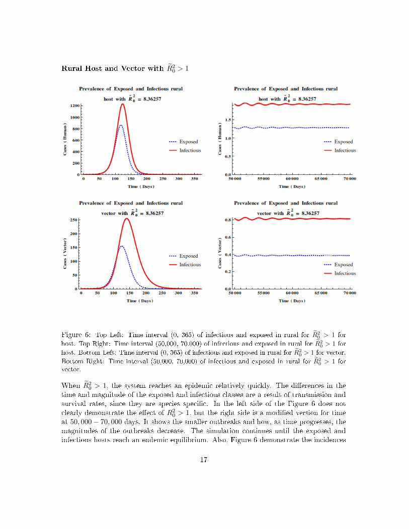
Figure 6: Top Left: Time interval (0, 365) of infectious and exposed in rural for R̃20 > 1 for

host. Top Right: Time interval (50,000, 70,000) of infectious and exposed in rural for R̃20 > 1 for

host. Bottom Left: Time interval (0, 365) of infectious and exposed in rural for R̃20 > 1 for vector.

Bottom Right: Time interval (50,000, 70,000) of infectious and exposed in rural for R̃20 > 1 for

vector.

When R̃20 > 1, the system reaches an epidemic relatively quickly. The di�erences in the

time and magnitude of the exposed and infectious classes are a result of transmission andsurvival rates, since they are species speci�c. In the left side of the Figure 6 does notclearly demonstrate the e�ect of R2

0 > 1, but the right side is a modi�ed version for timeat 50, 000− 70, 000 days. It shows the smaller outbreaks and how, as time progresses, themagnitudes of the outbreaks decrease. The simulation continues until the exposed andinfectious hosts reach an endemic equilibrium. Also, Figure 6 demonstrate the incidences

17

of DENV as time progresses in a rural population where R̃20 < 1, as time progresses, the

disease continues to exist with the magnitudes of the subsequent epidemics decreasing overtime. For this scenario, the transmission rates for rural susceptible hosts and vectors, βRand φR, are both set equal to 0.33. While the transmission rates for the susceptible urbanhost and vector, βU and φU , are both set equal to 0.31. All other parameters are speci�cto the host and vector species.

Urban Host and Vector with R̃20 < 1

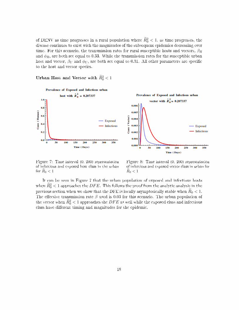
Figure 7: Time interval (0, 200) representationof infectious and exposed host class in the urbanfor R̃0 < 1

Figure 8: Time interval (0, 200) representationof infectious and exposed vector class in urban forR̃0 < 1

It can be seen in Figure 7 that the urban population of exposed and infectious hostswhen R̃2

0 < 1 approaches the DFE. This follows the proof from the analytic analysis in the

previous section when we show that the DFE is locally asymptotically stable when R̃0 < 1.The e�ective transmission rate β used is 0.03 for this scenario. The urban population ofthe vector when R̃2

0 < 1 approaches the DFE as well while the exposed class and infectiousclass have di�erent timing and magnitudes for the epidemic.

18

Urban Host and Vector with R̃20 > 1

Figure 9: Top Left: Time interval (0, 365) of infectious and exposed in Urban for R̃20 > 1 for host.

Top Right: Time interval (50,000, 70,000) of infectious and exposed in Urban for R̃20 > 1 for host.

Bottom Left: Time interval (0, 365) of infectious and exposed in Urban for R̃20 > 1 for vector.

Bottom Right: Time interval (50,000, 70,000) of infectious and exposed in Urban for R̃20 > 1 for

vector

5.1.2 Case with constant movement

We consider the case when we have constant movement between the population. Also, weassume that these constant do not change in the course of the epidemic. Numerical resultsshow that when R0 < 1, the host and vector do not move through the system and remainsusceptible. As in the urban area, the rural area also reaches a disease free equilibrium.Since DENV dies out, the system reaches a disease free equilibrium for this serotype, thisis, the infectious and exposed states decrease and eventually go to zero.

In the rural area, the disease follows a similar pattern to that of the urban area. Overtime, the disease reaches an endemic equilibrium for both the host and the vector. Thenumber of individuals in the exposed and infectious classes decrease over time, and a�ectthe rural area to smaller degree.

When R0 > 1, the system eventually reaches an endemic equilibrium. The numericalsimulations show future outbreaks, though they are smaller and occur with decreasing

19

magnitude over time. Similarly with hosts, when R0 > 1, the system reaches an endemicstate. The di�erences in the time and magnitude of the exposed and infectious classes area result of transmission and survival rates. Due to their short lifespan, as compared withthat of a host, the vector moves through the system much more quickly. Again, as timeapproaches in�nity, future outbreaks will lessen in both frequency and intensity.In the rural area, the disease follows a similar pattern to that of the urban area. Overtime, the disease reaches an endemic equilibrium for both the host and the vector. Thenumber of individuals in the exposed and infectious classes decrease over time, and a�ectthe rural area to smaller degree.

5.1.3 Case with function dependent movement

In this section, we show numerical simulations of the system with a change in the movementrates. The movement between the populations is analyzed with respect the proportion ofthe respective population. The dynamics between rural and urban population are com-pared. We consider the movement functions de�ned by

fR(I,N) = CR

(1−

(IHUNHU

− IHRNHR

))and

fU (I,N) = CU

(1−

(IHRNHR

− IHUNHU

)).

Rural Host and Vector with R20 < 1

Figure 10: Time interval (0, 200) representation of infectious and exposed vectors in rural forR0 < 1, φR = φU = .03 and βR = βU = .09

20

If R0 < 1, the disease transmission reach 0 cases for host and vector population in theinfectious and exposed states. The susceptible states (host and vector) reaches the total ofpopulation while the other cases go to 0, this is, we have stability in the DFE. We showtwo simulations with R0 < 1, in two of them the DFE is reached relatively quickly.

Rural Host and Vector with R0 > 1

Figure 11: Top Left: Time interval (0, 365) of infectious and exposed in rural for R0 > 1 forhost. Top Right: Time interval (50,000, 90,000) of infectious and exposed in rural for R0 > 1 forhost. Bottom Left: Time interval (0, 365) of infectious and exposed in rural for R0 > 1 for vector.Bottom Right: Time interval (50,000, 90,000) of Infectious and exposed in rural for R0 > 1 forvector

When R0 > 1 the epidemic is presented in a short period of time although the infectiousdoes not reach the zero value in rural nor urban population, this is a consequence oftransmission and survival rates in the vector. In both cases, the transmission rate for hostand vector are equal in the each area, βR = φR = .33 and βU = φU = .31. We assumein this case a greater transmission rate for the rural population, which is a�ected by theAe. aegypti. The di�erent magnitudes and initial times are exposed in order to show theconvergence of infectious and exposed states to the endemic equilibrium. In the right side

21

of the Figure 5.1.3 we show extension extensions in time of of the left side, in these plotswe observe a oscillated convergence to the endemic point where the amplitude decreasewhen t→∞. Also, we note that the convergence in the rural vector is faster that the hostpopulation, this is result of the survival rates.

Urban Host and Vector with R0 < 1

Figure 12: Time interval (0, 365) representationof infectious and exposed host class in the Urbanfor R0 < 1

Figure 13: Time interval (0, 365) representationof infectious and exposed vector class in the Ur-ban for R0 < 1

In the �gures above the urban populations (host and vector) are shown. Infectious andexposed states reach the disease free equilibrium ast → ∞, which is stable for R0 < 1.The transmission rate βR, βU , φR and φU change in each case, using βR = φR = .09 andβR = φR = .15 in the �rst graph, and βR = φR = .09 and βR = φR = .15 in the secondone. We also show two di�erent time scales in order to analyzed the convergence time withrespect to transmission rates.

22

Urban Host and Vector with R0 > 1

Figure 14: Top Left: Time interval (0, 365) of infectious and exposed in Urban for R0 > 1 forhost. Top Right: Time interval (40,000, 60,000) of infectious and exposed in Urban for R0 > 1 forhost. Bottom Left: Time interval (0, 365) of infectious and exposed in Urban for R0 > 1 for vector.Bottom Right: Time interval (40,000, 60,000) of infectious and exposed in Urban for R0 > 1 forvector

In the plots above the transmission rates are βR = φR = .33 and βR = φR = .31. In bothcases the infectious and exposed states converge to the endemic equilibrium. Both reachthe maximum value in the infectious states in a relatively short time.

The maximum number of infectious cases is small with respect to the initial conditionsfor the two populations.

23

6 Stochastic Simulations

6.1 Zero Movement

Figure 15: Infectious and exposed hosts, vectors where R̃0 < 1 and R̃0 > 1

In this section, simulations are done using a stochastic Markov process. The deterministicmodel is matched closely by the stochastic models, which suggests that the parametervalues are accurate means. Stochastic models were used only for the zero movement case.Infectious and exposed classes for hosts and vectors were examined for cases where R0 < 1and where R0 > 1. Stochastic models for the more complicated cases are not included asthey are extremely computationally expensive and ine�cient.

7 Cumulative Plots

Finally, we assess the cumulative amounts of infectious hosts for several scenarios. Initially,we consider the cases in which R0 < 1 for �ve simulations. The �rst simulation concerns asingle population of 10,000 hosts with no movement. The other four simulations concern

24

Figure 16: Cumulative infectious cases for multiple scenarios where the DFE is locallyasymptotically stable.

two host populations between which movement occurs. The two populations are a ruralpopulation of 2,000 hosts and an urban population of 8,000 hosts. The second and thirdsimulations consider cases of constant movement. In the second simulation, movementin both directions is equal, that is, CR = CU , while in the third simulation, CR > CU .Similarly, the last two simulations describe a case in which movement follows the functionsdescribed above, where movement is equal or preferential in the fourth and �fth simulations,respectively. When R0 < 1, all cases show stability at the disease free equilibrium, sothe disease dies out and the cumulative cases of infection reach a maximum and plateauthere. All scenarios reach their respective plateaus at approximately the same time. Thetotal cases of infection are greatest for the zero movement case and least for the cases ofpreferential movement, but in all cases, the total infectious cases are between 0.4 and 1.6cases.

Next, we consider the same scenarios for the case in which R0 > 1. When R0 > 1, allcases show stability at the endemic equilibrium, so the disease persists as new susceptibleindividuals enter the population and become infectious. In all cases, the disease eventu-ally a�ects e�ectively every member of the population, so the cumulative infectious casesapproach and plateau at 10,000 cases (the total host population for all simulations). Thescenarios reach this plateau at slightly di�erent times. The case of a single patch withzero movement is the �rst to reach the plateau, while the cases which include preferentialmovement are the last to reach the plateau. This is reasonable, as an outbreak spread morequickly in a single population of 10,000 than an outbreak which began in one populationand took time to travel to another population via host movement.

Analysis of the total infectious cases suggests while movement has some e�ect on theseverity (when R0 < 1) and speed (when R0 > 1) of a Dengue outbreak, it causes minimalpractical change. The greatest e�ect of host movement is its ability to spread Dengue to

25

Figure 17: Cumulative infectious cases for multiple scenarios where the endemic equilib-rium is stable.

new areas, rather than its ability to change other qualitative traits of an outbreak.

8 Discussion

The purpose of this paper is to model the spread of Dengue fever, taking into considerationmovement between rural and urban areas. It is assumed that urban and rural vectors donot leave their respective areas and will only bite mobile hosts. The total populations ofvectors, NV R and NV U , are constant, as is the total population of hosts, NH . The hostsubpopulations, NHR and NHU , are not constant when movement occurs. It is assumedthat exposure to DENV does not impede or change movement in the host, but someproportion of the infectious class is immobile and therefore also unable to be bitten by andinfect susceptible vectors. The model considers only one serotype, to which all recoveredhosts are permanently immune. Finally, the model considers the populations of hosts andvectors to be homogeneously mixed, so that any mobile host has an equal probability ofbeing bitten by any vector in that area.

In the deterministic model, the simulations show that when R0 < 1, DENV reachesthe disease free equilibrium for both the host and vector. The infectious and exposedclasses slightly increase, but infectious individuals leave the class via recovery or naturaldeath before infecting an average of one host or vector. Also, the deterministic modelsdemonstrate the existence of an endemic equilibrium. At the endemic equilibrium, thedisease is present in the population but does not cause disturbance. Many subtropicaland temperate regions undergo seasonal endemics; however, with an increased tendencyfor hosts to travel, this can quickly lead to an epidemic in multiple areas. The numericalsimulations suggest that over a very long time period, the outbreaks of Dengue become

26

more infrequent and decrease in magnitude. Damping oscillations occur as the populationsapproach the endemic equilibrium, when R0 > 1.

In addition to the deterministic model, we also constructed a stochastic model in orderto con�rm the accuracy of our parameters by adding randomness to the model. Thedeterministic model is used to make predictions based on average parameters and theschematics of the system. This type of model allows us to understand the basic dynamicsof transmission where the state variables follow a �ow chart and depend on previous states.On the other hand, the stochastic model incorporates a memoryless tool that contributes tothe model's realistic outputs. The transmission rates of Dengue between hosts and vectorsare dependent on random occurrences, which is re�ected in the stochastic model. Finally,it allows us to observe many di�erent qualitative outcomes as well as the probabilities ofeach outcome. Plotting the stochastic and deterministic models together shows that thedeterministic model is the approximate average of the stochastic plots, which supports theaccuracy of our model.

In conclusion, we notice that the transmission rates β and φ are directly proportionalto R0, such that an increase in the transmission rates will result in an increase in R0.We modeled the dynamics of Dengue transmission with host movement between rural andurban areas and observed the e�ects on transmission between the hosts and the stationaryvectors. We conclude that while movement between rural and urban areas does not have anotable e�ect on the speed or severity of a Dengue outbreak in one area, host movement issolely responsible for the spread of Dengue to new areas and populations. Analysis of thesystem both with and without movement did not reveal a major change in transmissiondynamics due to the addition of movement.

For future studies, we will model movement with time-dependent rates. In the future,we also would consider the potential e�ects of a vaccination, for which we would need totake into account all separate serotypes of DENV. If multiple serotypes are included in afuture model, we would also consider instances of DSS as a result of secondary infection,as well as disease-related death.

9 Acknowledgments

We would like to thank Dr. Carlos Castillo-Chavez, Executive Director of the Mathematicaland Theoretical Biology Institute (MTBI), for giving us this opportunity to participate inthis research program. We would also like to thank Co-Executive Summer Directors Dr.Omayra Ortega and Dr. Baojun Song for their e�orts in planning and executing the dayto day activities of MTBI. This research was conducted in MTBI at the Simon A. LevinMathematical, Computational and Modeling Sciences Center (SAL MCMSC) at ArizonaState University (ASU). This project has been partially supported by grants from theNational Science Foundation (DMS-1263374 and DUE-1101782), the National SecurityAgency (H98230-14-1-0157), the O�ce of the President of ASU, and the O�ce of theProvost of ASU.

27

Special thanks to our faculty advisors Dr. Fabio Sanchez and Dr. Omayra Ortega.We would like to express our appreciation for the wisdom and continuous encouragementfrom our graduate mentors Komi Messan and I Made Eka Dwipayana, as well as Dr. AbbaGumel and Dr. Susan Holechek. We also thank Dr. Ricardo Sá enz for his insight andsuggestions.

28

A.10 Appendix

In this appendix we give some mathematical results that are not shown in the previoussections.

A.10.1 Basic Reproductive Number

A.10.1.1 Case without movement

To �nd the reproductive number R̃0, we follow the Next Generation Operator MatrixMethod [28]. F represents the rate of the new infections caused by transition to theinfectedgroup. V represents the rates of transfer of individuals into or out of the infected classesby other means. This is,

F =

βSH

IVNV

φSV pIHNH

00

and V =

αEH + µHEHθEV + µVEV

−αEH + δEV + µHEVθEV + µV IV

.

The partial derivatives of each matrix are taken with respect to the variables representingthe new exposed and infectious classes. Both matrices will be evaluated at the DFE,resulting in

F =

0 0 0 β SHNV0 0 φp SVNV 0

0 0 0 00 0 0 0

and V =

α+ µH 0 0 0

0 θ + µV 0 0−α 0δ + µH 0 00 −θ 0 µV

.

We determine the spectral radius of FV −1. Then, the basic reproductive number is

R̃0 = ρ(FV −1) =

√β

δ + µH· φpµV· θ

µV + θ· α

α+ µH

A.10.1.2 Constant movement case: fU (I,N) = CU and fR(I,N) = CR.

We use the next generation operator matrix method to calculate the basic reproductivenumber and analyze local stability of the DFE. The vector X consists of infected classesand Y of all other classes are given by:

29

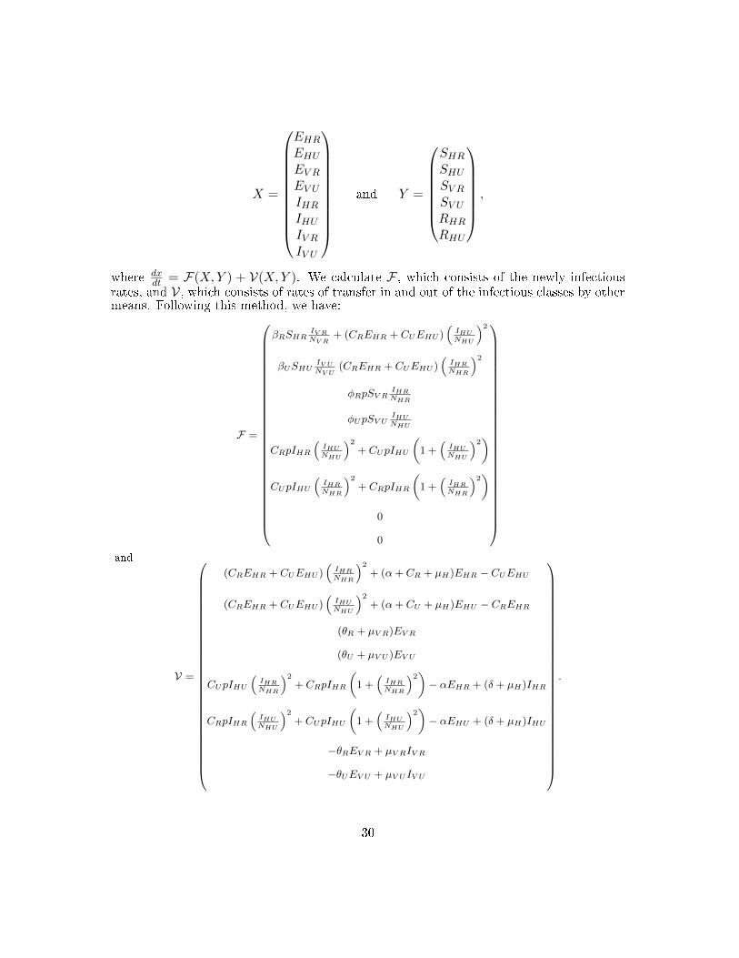
X =

EHREHUEV REV UIHRIHUIV RIV U

and Y =

SHRSHUSV RSV URHRRHU

,

where dxdt = F(X,Y ) + V(X,Y ). We calculate F , which consists of the newly infectious

rates, and V, which consists of rates of transfer in and out of the infectious classes by othermeans. Following this method, we have:

F =

βRSHRIV RNV R

+ (CREHR + CUEHU )(IHUNHU

)2βUSHU

IV UNV U

(CREHR + CUEHU )(IHRNHR

)2φRpSV R

IHRNHR

φUpSV UIHUNHU

CRpIHR(IHUNHU

)2+ CUpIHU

(1 +

(IHUNHU

)2)

CUpIHU(IHRNHR

)2+ CRpIHR

(1 +

(IHRNHR

)2)0

0

and

V =

(CREHR + CUEHU )(IHRNHR

)2+ (α+ CR + µH)EHR − CUEHU

(CREHR + CUEHU )(IHUNHU

)2+ (α+ CU + µH)EHU − CREHR

(θR + µV R)EV R

(θU + µV U )EV U

CUpIHU(IHRNHR

)2+ CRpIHR

(1 +

(IHRNHR

)2)− αEHR + (δ + µH)IHR

CRpIHR(IHUNHU

)2+ CUpIHU

(1 +

(IHUNHU

)2)− αEHU + (δ + µH)IHU

−θREV R + µV RIV R

−θUEV U + µV UIV U

.

30

Then, we take the partial derivatives with respect to the infectious classes, X, and evaluateat the DFE.

F =

0 0 0 0 0 0 βRNHRNV R

0

0 0 0 0 0 0 0 βUNHUNV U

0 0 0 0 φRpNV RNHR

0 0 0

0 0 0 0 0 φUpNV UNHU

0 0

0 0 0 0 0 0 0 00 0 0 0 0 0 0 00 0 0 0 0 0 0 00 0 0 0 0 0 0 0

and

V =

CR + α+ µH −CU 0 0 0 0 0 0−CR CU + α+ µH 0 0 0 0 0 00 0 θR + µV R 0 0 0 0 00 0 0 θU + µV U 0 0 0 0−α 0 0 0 δ + µH 0 0 00 −α 0 0 0 δ + µH 0 00 0 −θR 0 0 0 µV R 00 0 0 −θU 0 0 0 µV U

.

The next generation matrix is FV −1 where ρ(FV −1) is the basic reproduction number,R0. The R0 is given by:

R0 =1

2

(R̃2

0R+ R̃2

0U

)+

√14

(CU+α+µH

CR+CU+α+µHR̃2

0R− CR+α+µH

CR+CU+α+µHR̃2

0U

)2+(CRR̃2

0R

)(CU R̃2

0U

)

where

R̃20R

=βR

µH + δ· φRpµV R

· θRµV R + θR

· α

α+ µH

R̃20U

=βU

µH + δ· φUpµV U

· θUµV U + θU

· α

α+ µH

31

References

[1] Gubler D.J. Sie A. Suharyono W.-Tan R. Abidin, M. Viraemia in patients with natu-rally acquired dengue infection. Bulletin of the World Health Organization, 59:623�630,1981.

[2] Che Salmah M. Norasmah B.-Nur Aida H. Nurita A. Abu Hassan, A. Populationanalysis of Aedes albopictus (skuse) (diptera: Culicidae) under uncontrolled laboratoryconditions. Tropical Biomedicine, 25:117�125, 2008.

[3] Chompoosri J. Siriyasatien P. Tawatsin A.-Thavara U. Anantapreecha, S. Seasonalmonitoring of dengue infection in Aedes aegypti and serological feature of patients withsuspected dengue in 4 central provinces of thailand. The Thai Journal of VeterinaryMedicine, 42(2):185�193, 2013.

[4] Nisalak A. Watts D.M. Whitmore R.E.-Harrison B.A. Burke, D.S. E�ect of temper-ature on the vector e�ciency of Aedes aegypti for dengue 2 virus. American Journal

of Tropical Medicine and Hygiene, 36:143�152, 1987.

[5] Liao Chio C.M. Chio C.P. Hsiao-Han C. You S.H. Cheng Y.H. Chen, S.C. Laggedtemperature e�ect with mosquito transmission potential explains dengue variability insouthern taiwan: insights from a statistical analysis. Science of the total environment,408(19):4069�4075, 2010.

[6] Dumont Y. Chiroleu, F. Vector control for the chikungunya disease. Mathematical

Biosciences and Engineering, 7(2):315�348, 2010.

[7] Cushing J. Hyman J. Chitnis, N. Determining important parameters in the spreadof malaria through the sensitivity analysis of a mathematical model. Bulletin of

Mathematical Biology, 70(5):1272�1296, 2008.

[8] Haussermann W. Trpis M. Craig, G.B. Estimates of population size, dispersal, andlongevity of domestic Aedes aegypti by mark-release-recapture in the village of shaurimoyo in eastern kenya. Journal of Medical Entomology, 32:27�33, 1995.

[9] Focks D.A. Garcia A.J. Morrison A.C. Ellis, A.M and T.W. Scott. Parameteriza-tion and sensitivity analysis of a complex simulation model for mosquito populationdynamics, dengue transmission, and their control. The American journal of tropical

medicine and hygiene, 85(2):257�264, 2011.

[10] Ennis F.A. Green S. Innis B.L.-Kalayanarooj S. Nisalak Nimmannitya S. Raengsakul-rach B. Rothman A.L. Suntayakorn S. A. Vaughn D.W. Endy, T.P. Dengue viremiatiter, antibody response pattern, and virus serotype correlate with disease severity.Journal of Infectious Diseases, 181:2�9, 2000.

32

[11] Lourdes Esteva and Cristobal Vargas. Analysis of a dengue disease transmission model.Mathematical biosciences, 150(2):131�151, 1998.

[12] Lourdes Esteva and Cristobal Vargas. A model for dengue disease with variable humanpopulation. J. Math. Biol., 38:220�240, 1999.

[13] Lourdes Esteva and Cristobal Vargas. Coexistence of di�erent serotypes of denguevirus. Journal of Mathematical Biology, 46(1):31�47, 2003.

[14] Centers for Disease Control and Prevention. Dengue and the aedes albopictusmosquito, January 2012.

[15] Centers for Disease Control and Prevention. Dengue, June 2014.

[16] Salisu Mohammed Garba, Abba B Gumel, and Mohd Rizam Abu Bakar. Backwardbifurcations in dengue transmission dynamics. Mathematical biosciences, 215(1):11�25, 2008.

[17] Hitchens A.P. Siler J.F. Hall, M.W. Dengue: the history, epidemiology, mechanism oftransmission etiology, clinical manifestations, immunity, and prevention. Philippine

Journal of Science, 29:1�304, 1926.

[18] Trpis M. Haussermann, W. Dispersal and other population parameters of Aedes ae-gypti in an african village and their possible signi�cance in epidemiology of vector-borne diseases. American Journal of Tropical Medicine and Hygiene, 35:1263�1279,1986.

[19] Jennifer L Kyle and Eva Harris. Global spread and persistence of dengue. Annu. Rev.Microbiol., 62:71�92, 2008.

[20] Pradhan S.K. Lahariya, C. Emergence of chikungunya virus in indian subcontinentafter 32 years: a review. Journal of Vector Borne Diseases, 43(4):151, 2006.

[21] Kyle S. Hickmann Sen Xu-Helen J. Wearing James M. Hyman Manore, Carrie A.Comparing dengue and chikungunya emergence and endemic transmission in A. ae-

gypti and A. albopictus. May 2014.

[22] Dennis Normile. Surprising new dengue virus throws a spanner in disease controle�orts. Science, 342(6157):415, 2013.

[23] Alongkot Ponlawat and Laura C Harrington. Blood feeding patterns of Aedes aegyptiand Aedes albopictus in thailand. Journal of medical entomology, 42(5):844�849, 2005.

[24] Megan E Reller, Champika Bodinayake, Ajith Nagahawatte, Vasantha Devasiri, Was-antha Kodikara-Arachichi, John J Strouse, Anne Broadwater, Truls Østbye, Aravindade Silva, and Christopher W Woods. Unsuspected dengue and acute febrile illness

33

in rural and semi-urban southern sri lanka. Emerging infectious diseases, 18(2):256,2012.

[25] S.B. Sabin. Research on dengue during world war ii. American Journal of Tropical

Medicine and Hygiene, 1:30�50, 1952.

[26] Macdonald W.M. Tonn R.J. Grabs B. Sheppard, P.M. The dynamics of an adultpopulation of Aedes aegypti in relation to dengue haemorrhagic fever in bangkok.Journal of Animal Ecology, 38:661�701, 1969.

[27] Maria da Glória Teixeira, Maurício L Barreto, Maria da Conceição N Costa, LeilaDenize A Ferreira, Pedro FC Vasconcelos, and Sandy Cairncross. Dynamics of denguevirus circulation: a silent epidemic in a complex urban area. Tropical Medicine &

International Health, 7(9):757�762, 2002.

[28] Pauline Van den Driessche and James Watmough. Reproduction numbers and sub-threshold endemic equilibria for compartmental models of disease transmission. Math-

ematical biosciences, 180(1):29�48, 2002.

[29] Sirenda Vong, Virak Khieu, Olivier Glass, Sowath Ly, Veasna Duong, Rekol Huy,Chantha Ngan, Ole Wichmann, G William Letson, Harold S Margolis, et al. Dengueincidence in urban and rural cambodia: results from population-based active feversurveillance, 2006�2008. PLoS neglected tropical diseases, 4(11):e903, 2010.

[30] K. Walker. Asian tiger mosquito (Aedes albopictus). Pest and Diseases Image Library,2007.

[31] Annelies Wilder-Smith and Duane J Gubler. Geographic expansion of dengue: theimpact of international travel. Medical Clinics of North America, 92(6):1377�1390,2008.

[32] Catherine Zettel and Phillip Kaufman. Yellow fever mosquito Aedes aegypti (lin-naeus)(insecta: Diptera: Culicidae), 2012.

34