The Effect of Collusion on Efficiency in

Experimental Auctions

Charles N. Noussair∗ Gyula Seres†

February 21, 2017

Abstract

This paper examines the effect of collusion on allocative efficiencyin a second-price sealed-bid auction, in which bidders’ valuations haveprivate and common value components. We present a theoretical modelwhich shows that explicit collusion improves average efficiency. Fur-thermore, a reduction in common value signal variance increases theefficiency of allocations when a cartel is present. We test for the pres-ence of these patterns in a laboratory experiment. Subjects can choosewhether to compete or to form a cartel. Colluding bidders can commu-nicate and make side payments using a knockout auction. Our resultsshow that a large majority of bidders join a cartel, collusion has anegative impact on efficiency, and a reduction in common value signalvariance increases efficiency under a cartel, as well as in a competitivesetting.

JEL Codes: D44, D82, L41, C92Keywords: Auction; Bidding ring; Information asymmetry; Experiment

1 Introduction

In an auction market for a single good, full ex post allocative efficiency isachieved if the player with the highest valuation is awarded the item. When

∗University of Arizona, Eller College of Management, Economic Science Laboratory.Email: cnoussair@email.arizona.edu†Humboldt University Berlin, Faculty of Economics and Business Administration.

Email: gyula.seres@hu-berlin.edu. We thank the CentER for Economic Research atTilburg University for financial support. We are grateful to Jan Boone, Jacques Cremer,Eric van Damme, Theo Offerman, Jan Potters, Nicholas Treich, as well as participantsat the Experimental Economics Meeting at Tilburg University and at the EARIE 2016Conference for their valuable comments.

1

bidders’ valuations for a good are known at the time of bidding, even whenthey are only privately known, it is typically straightforward to achieve anefficient allocation with a number of different auction rules (Vickrey, 1961).When the valuations are correlated, such as in the generalized mineral rightsauction defined by Milgrom and Weber (1982), efficiency is also easy toachieve (Jehiel and Moldovanu, 2001). If the item sold has a common valueto all bidders, even if the value of the item is not known at the time ofbidding, it is equally efficient to allocate the unit to any demander, so thatpreventing inefficiency is a trivial matter.

However, consider an environment in which bidders’ private informationconsists of a private value component, known with certainty, as well as asignal about a common value component. This structure is, for example,a plausible way to model how individuals value artwork, which is typicallysold by auction. A bidder has an intrinsic preference for the painting basedon her private tastes, the private value component, but may also have beliefsabout the price at which the item can potentially be resold in the future,a noisy common value signal. Other items sold in auctions, such as realestate, automobiles, and concert tickets have a similar feature, in that theyhave a private use value, as well as common future market value that maybe unknown at the time of bidding. Yet another example is constructionprocurement, in which bidders are sellers rather than buyers. Some costsare uncertain but common to all bidders, for example the market prices forinputs such as fuel or cement, but the cost effects of some inputs includingexperience or access to capital are private and vary by bidder.

In these situations, for an efficient allocation to occur, the bidder withthe highest private value must receive the item. Nevertheless, it is possiblefor an auction system, even one that always awards the item to the highestbidder, to allocate an item inefficiently, despite all bidders behaving opti-mally. This is because an individual with a low private value but a commonvalue signal that happens to be much higher than the true common valuecomponent might submit the highest bid.1 In general, no efficient, incen-tive compatible mechanism exists if types are multi-dimensional (Jehiel andMoldovanu, 2001).

If bidders could obtain more precise estimates of the common value, theextent of inefficiency could be reduced. One way to potentially allow this tohappen is to permit bidders to collude. As noted by Groenewegen (1994)

1The winner’s curse is not the source of the inefficiency. Equilibrium bidding strategiesof rational bidders also results in efficiency loss. Goeree and Offerman (2002) find experi-mental evidence that naive bidding itself does not have a significant impact on efficiency.

2

and Goeree and Offerman (2003), collusion with the possibility of explicitcommunication is actually beneficial for allocative efficiency. It is commonlyaccepted that cartels have a detrimental effect on the seller’s revenue, but anincrease in overall efficiency would provide a rationale for permitting biddercollusion.2

We examine this issue in this paper, where we report a laboratory ex-perimental study on second-price auctions. The source of our hypotheses isa theoretical model assuming rational bidders. The model yields the resultthat collusion increases expected allocative efficiency. The intuition stemsfrom information sharing that occurs during the collusion process. Thissharing increases the likelihood that the bidder with the highest valuation ischosen to submit the highest bid. The model also predicts that all potentialbidders join the cartel, and that an exogenous reduction in common valueuncertainty increases allocative efficiency, given that a cartel is formed.

Our experiment consists of four treatments. In the first two treatmentsof the study, there are two potential bidders who can decide to collude be-fore the auction takes place. Their valuations consist of private and commonvalue components. The difference between the two treatments is the spreadof the common value distribution. The LoVar treatment has a lower com-mon value variance than HiVar. Comparison of these two treatments testsan implication of our model. It also addresses a question of whether anauthority interested in efficiency should make public any information it hasthat might reduce common value uncertainty.3 A third treatment, NoColl,has the same parametric structure as HiVar, but collusion is prohibited.Comparison of HiVar and NoColl provides a measure of the consequencesof prohibiting collusion. In a fourth treatment, PVOnly, bidders’ valuationsconsist of only a private value component. In PVOnly, at least accordingto our model, collusion can provide no additional efficiency, since there isno common value uncertainty to resolve. If the process of collusion tends tointroduce inefficiencies that are unanticipated in our model, collusion wouldlower efficiency in this treatment.

We observe substantial support for a number of the predictions of the

2This argument was made by members of the long-standing Dutch construction car-tel, who testified in 2002 that the primary motivation of their operation as a cartel wasinformation pooling (Boone, Chen, Goeree, and Polydoro, 2009). For details of the par-liamentary hearings, see Parlementaire Enquetecommissie Bouwnijverheid (2003).

3Milgrom and Weber (1982) show that an auctioneer can increase revenue by releasingany private information she has that can reduce common value uncertainty on the partof bidders. In the context of our motivating example, the auctioneer in a constructionprocurement auction typically has private information about the construction site, relatedprojects, or estimated cost.

3

model. A large majority of bidders attempt to form a ring. Treatments withdifferent variance of the common value signal produce the result predictedby the model, which is that more variance leads to greater efficiency loss.However, we also find that cartels fail to increase efficiency. Imperfectionsin the process of assigning the designated bidder and the side payment tothe other bidder at times fails to make an efficient assignment. This morethan offsets the gain in efficiency from the information sharing among car-tel members. In the PVOnly treatment, where there is no common valueuncertainty, and thus no gain from pooling information, bidding rings re-duce efficiency substantially. We also observe that if cartels are prohibited,outcomes differ from a situation in which bidders voluntarily decline theopportunity to form a cartel. They bid more aggressively if cartels are in-terdicted.

The work reported here fits into the large literature initiated by Ver-non Smith and his colleagues on using laboratory experiments to evalu-ate game-theoretic models of auctions (Coppinger, Smith, and Titus, 1980;Cox, Smith, and Walker, 1982). This literature has diverged in a numberof directions in the last three decades. One currently active avenue hasbeen the investigation of collusion in auctions. Recent lines of research ad-dress leniency programs (Bigoni, Fridolfsson, Le Coq, and Spagnolo, 2015;Apesteguia, Dufwenberg, and Selten, 2007; Hinloopen and Soetevent, 2014),cartel detection (Hinloopen and Onderstal, 2014), communication within thecartel (Agranov and Yariv, 2016; Llorente-Saguer and Zultan, 2014) and theeffect of reference prices (Armantier, Holt, and Plott, 2013).

The paper is structured as follows. Section 2 describes the model, andcharacterizes an equilibrium with risk neutral, rational bidders. Details ofthe experimental design are given in Section 3. Section 4 formally states ourhypotheses. Section 5 reports our data analysis and summarizes our results.Finally, Section 6 concludes with a discussion.

2 Model and equilibrium

In this section, we analyze the auction game that we study in our experi-ment. The game proceeds in a number of stages. Nature chooses the privateinformation of the three bidders who have the right to participate in the auc-tion. Two of the bidders then choose whether or not to create a biddingring. If a ring is created, the ring members use a bidding process called aknockout auction (Mailath and Zemsky, 1991) to determine who will be thedesignated bidder in the subsequent main auction, and the side payment

4

that the other ring member receives in exchange for withdrawing from themain auction. The designated bidder then participates in the main auctionagainst the third bidder.

The environment is one in which bidders’ valuations for the item haveboth a private value and a common value component, as in Goeree andOfferman (2003). The private value component is known with certainty,and bidders have unbiased signals about the common value component. Theauction follows second-price sealed-bid rules. In the pure-strategy perfectBayesian equilibrium to the game that we derive, players always form acartel, and the cartel agrees on a transfer from the designated bidder to thewithdrawn bidder equal to half of the expected payoff that the withdrawnbidder would receive in main auction in the event that he were the designatedbidder.4

2.1 Model

Two strong and one weak bidder have valuations for an item sold in a second-price sealed-bid auction. The strong bidders i and j are symmetric andrisk neutral. Strong bidders’ valuations consist of two additively separablecomponents: a private value (PV) and a common value (CV). The privatevalue of each strong bidder i, denoted by xi, is drawn independently froma uniform distribution on [xL, xH ]. The common value component y is theaverage of the two strong bidders’ independently and identically distributedcommon value signals, denoted as yi and yj . The signals are each drawnfrom a uniform distribution, so that yi ∈ [yL, yH ]. The distributions ofprivate values and common value signals are common knowledge. Thus, thevaluation of bidder i, denoted by vi, has the structure shown in Equation(1).

vi = xi + y = xi +yi2

+yj2

(1)

The third bidder, called l, is weak in the following sense. Her valuationconsists entirely of a private value component, c, drawn from a uniformdistribution with support c ∈ [cL, cH ], where cL ≤ xL, cH ≤ xH . We assumethat cL, xL and yL are all non-negative.

4This form of collusion is a strong cartel in the sense of McAfee and McMillan (1987),who define a strong cartel as one that can specify and enforce side payments between ringmembers. It is also a strong cartel in the sense of Marshall and Marx (2007), in that itcan enforce a restriction that only the designated bidder submits a meaningful bid.

5

Bidders participate in a second-price sealed-bid auction. Bids are sub-mitted simultaneously. The player submitting the highest bid is awardedthe item for a price equal to the second highest bid. If there is a tie for thehighest bid, the tie is broken randomly. Before the auction, the two strongbidders can form a cartel by mutual agreement. The game consists of thefollowing sequence of events.

1. Nature chooses bidders’ private values and common value signals: xi,yi xj , yj , and c.

2. The strong bidders decide whether or not to form a bidding ring. Theymake their choices simultaneously. A cartel is formed if they bothchoose to join. Otherwise, no cartel is formed and the game proceedsto Stage 4.

3. If a bidding ring is formed, the cartel members participate in a knock-out auction and simultaneously submit their knockout bids ki and kj .The higher bidder is awarded the right to participate in the subse-quent main auction. This designated bidder pays the lower of the twoknockout bids to the other ring member, who is forced to bid 0 in themain auction.5 Ties are broken randomly. Knockout bids are observedby both members of the ring.

4. The main auction takes place, following second-price, sealed-bid auc-tion rules. If a cartel is formed, the auction has two active bidders, thedesignated bidder and the weak bidder. If no ring is created, there arethree bidders in the main auction, the two strong and the one weakbidder.

2.2 Equilibrium analysis

In this subsection, we derive a perfect Bayesian equilibrium to the game. Weassume that the two strong bidders use the same strategy. In Subsections2.2.1 and 2.2.2, we consider the subgames in which no bidding ring is formed,and in which one is formed, respectively. In Subsection 2.2.3, we analyze theknockout auction, and in Subsection 2.2.4, we consider the decision aboutwhether or not to collude. We show that all bidders benefit from collusion.In Subsection 2.2.5, we derive two results regarding allocative efficiency. Weshow that efficiency is greater on average when collusion is permitted than

5The partnership dissolution literature refers to a related mechanism as a Loser’s BidAuction (Li, Xue, and Wu, 2013).

6

when it is not. We also establish that efficiency is higher when commonvalue uncertainty is smaller. We solve the game by backward induction,beginning with the main auction in Stage 4.

2.2.1 The main auction without collusion

Consider the subgame reached in the last stage of the game if the strong bid-ders choose not to collude.6 We shall refer to this situation as a competitiveauction. In this subgame, players place bids in the main auction indepen-dently and competitively. Define the composite signal of strong bidder i assi = xi + yi

2 . The optimal bid of a player is a function of her composite sig-nal.7 To see this, note that the valuation of bidders consists of the compositesignal, which is known to the bidder at the time of bidding, and an unknownpart yj/2. The private value auction is a special case of this environment, inwhich si = xi and player i has a dominant strategy to submit a bid of xi, asin Vickrey (1961). However, the existence of a dominant strategy does notcarry over to auctions with common value uncertainty, and a strong bidder’sbest response depends upon the strategy the other strong bidder uses.8

Consider a Bayesian equilibrium b∗ = (b∗i (xi, yi) , b∗j (xj , yj) , b

∗l (c)) to

this subgame, where b∗i is the bidding strategy of bidder i. Strong bidder i’sequilibrium strategy is given by Equation (2).

b∗i (xi, yi) = E (vi|si = sj) = si +1

2E (yj |si = sj) (2)

with a similar strategy employed by bidder j. In words, bidder i bids anamount equal to her expected valuation conditional on bidder j having anidentical composite signal. To see this, first note that bidder i wishes tosubmit the highest bid and win the auction in all cases in which her com-posite signal is greater than that of the other two bidders. In cases in whichher composite signal is not the highest, she would prefer not to outbid theother player and win the auction. Her willingness-to-pay is then equal toher expected valuation for the item. However, her valuation depends on the

6As we shall see later, this stage is reached with probability 0 in equilibrium. We assumethat the out-of-equilibrium beliefs about other players’ private values and common valuesignals are the same as the initial priors.

7The following derivation is similar to the one given in Goeree and Offerman (2003).They refer to the composite signal as surplus.

8Consider a bidder with a very low composite signal. Conditional on winning, the CVof the other bidder is also low. For a higher composite signal, the CV of the other bidderis not similarly constrained. Consequently, the equilibrium bidding strategy is typically apiecewise linear function of si.

7

other player’s composite signal, because one component of player i’s valua-tion is yj . The greater the value of yj , the greater is sj , and the greater isvi as well. Thus, the region in which player i wins the auction profitably isthe region in which she pays less than [vi|si = sj ]. The weak player submitsa bid equal to her valuation c, which is her dominant strategy.

2.2.2 The main auction with collusion

We now analyze the subgame in which the main auction takes place after theformation of a cartel. Assume that bidder i has won the knockout auctionand is the designated bidder. She is then in a two-player auction facing theweak bidder. The information she has available is (xi, yi) and the knockoutbid of the other ring member kj . In equilibrium, bidder i updates her beliefabout the type of j, and in turn her own valuation. Her equilibrium bid inthe auction is derived in an analogous manner to (2) and equals:

d∗i (xi, yi) = xi +yi2

+1

2E (yj |kj) = si +

1

2E (yj |kj) . (3)

2.2.3 Knockout auction

We now turn to the knockout auction in Stage 3. To derive the equilibriumknockout bids of the subgame with collusion, note that they are determinedby the expected payoff that the agent can earn if she is the designated bidderin the subsequent main auction. A bidder would rather lose the knockoutauction if she receives at least as much in a side payment as her expectedpayoff in the main auction, and would like to win the knockout auction ifshe can do so at a price less than her expected payoff in the main auction.Thus, her optimal bid in the knockout auction is a function of her expectedpayoff given her composite signal, and conditional on winning the knockoutauction. Given the strictly monotonic relationship between the compositesignal and the knockout bid, the designated bidder learns the compositesignal of the other strong bidder after the knockout auction is completed.

We denote the expected payoff of i in the main auction as Π (si) =EΠ (si|si ≥ sj), where Π (·) refers to the expected revenue of i facing onlythe weak bidder. The equilibrium knockout bid is half of this value. Thereason is that unlike in the standard second-price auction, the loser receivesher own bid. That is, in equilibrium, conditionally on facing an identicalopposing bid, the bidder must be indifferent between (a) being the winnerof the knockout auction and continuing on to the main auction, and (b)

8

receiving the side payment. Therefore, i bids

k∗i (si) =1

2EΠ (si) =

1

2EΠ(si|si ≥ sj). (4)

2.2.4 The collusion decision

We now consider the decision of a bidder, taken in Stage 2, regarding whetheror not to collude. This binary decision is denoted by e ∈ {0, 1}, where 1refers to joining the ring. The expected payoff of a bidder engaging incollusion is∫ si

sj=xL+yL2

(Π (si)−

1

2Π (sj)

)d H (sj) +

∫ xH+yH2

sj=si

1

2Π (si) d H (sj) (5)

conditionally on all bidder types joining the ring, where H(sj) refers to theex ante distribution of the composite signal. The term on the left describesthe payoff in the event of winning the knockout auction, while the term onthe right corresponds to losing the knockout auction and receiving the sidepayment.

We provide a sufficient condition under which this total expected payofffrom collusion is higher than the conditional interim expected payoff in acompetitive auction, for all bidder types. If the condition is satisfied, allbidders would collude, regardless of their private information. ExpressionΠ(si) denotes the expected payoff of a bidder in a competitive auction. Weneed to show that

Π(si) ≤ E[max

{1

2Π(si), Π(si)−

1

2Π(sj),

}](6)

where the expectations are over the type of the other bidder. If 12Π(si) −

12Π(sj) ≥ 0, rearranged, we get

Π(si)−1

2Π(si) ≤

1

2Π(si)−

1

2Π(sj) (7)

If 12Π(si)− 1

2Π(sj) < 0, we get

Π(si)−1

2Π(si) ≤ 0 (8)

Since the right-hand sides of inequalities (7) and (8) are non-negative, it isa sufficient condition, that Π(si) − 1

2Π(si) ≤ 0 ⇐⇒ Π(si) ≥ 2Π(si). Ourfindings are summarized in Proposition 1.

9

Proposition 1. All bidder types join the ring, e∗(si) = 1, if Π(si) ≥ 2Π(si).

That is, all bidder types participate if competition can be successfully sup-pressed. This condition is satisfied in all treatments of our experimentaldesign.

The arguments presented above show that there exists an equilibriumwith the following structure.9

e∗i (si) = 1 (9)

d∗i (si) = si +1

2E (yj |kj) (10)

k∗i (si) =1

2EΠ(si|si ≥ sj) (11)

b∗i (si) = si +1

2E (yj |si = sj) (12)

b∗l (c) = d∗l (c) = c (13)

with bidder j employing the same strategy as i.

2.2.5 Theoretical results regarding efficiency

Ex post efficiency is guaranteed in a pure common value auction, since valu-ations are identical. In a symmetric pure private value auction, equilibriumbids increase in valuation, and this guarantees that the efficient buyer ob-tains the commodity. Inefficiencies might appear if both types of informationasymmetry are present, as Goeree and Offerman (2003) argue.

A bidder with high PV and low CV might bid lower in equilibrium thanan opponent with low PV and high CV. For example, consider two strongbidders, with types (xi = 800, yi = 0) and (xj = 700, yj = 400), where thesupports of PV and CV signals are [0, 800] and [0, 400], respectively. Theweak bidder bids c = 500. In equilibrium, player i submits b∗i = 900, whereasb∗j = 1050. Bidder j wins the auction, while her opponent has higher PV,resulting in an efficiency loss of xi − xj = 800− 700 = 100.

9There is clearly a multiplicity of equilibria in this game. Consider for instance thesame strategy profile ,with one modification. Bidder i, conditionally on reaching the mainauction as a designated bidder, submits an arbitrarily high bid if si > cH . However,equilibria of this type leads to the same payoffs as the one we have derived, in that acartel is always formed, the bidder with the highest valuation is always the designatedbidder, and the prices in the knockout and main auctions, as well as the final allocation,are the same.

10

The ranking of knockout bids and competitive auction bids of the strongbidders coincide, since bids are monotonic in composite signals in both thecompetitive and the knockout auctions. However, the information containedin the knockout bids help the designated bidder to improve her beliefs re-garding the CV signal of the other ring member, as we have also seen above,

bidding si +E(yj |kj)

2 . This bid equals the expected valuation of the bidder,where the distribution of beliefs second-order stochastically dominates thatof the competitive bidder. This means that the probability of winning, con-ditional on having a valuation greater than that of the weak bidder, is alsogreater than in the competitive auction. These arguments are summarizedin Proposition 2.

Proposition 2. Collusion has no effect on the allocation of the good betweenthe strong players. The overall probability of an efficient allocation is higherif a bidding ring is formed.

Proof. The first part of the proposition is a consequence of the monotonicityof bids in composite signals in the competitive auction, and the fact thatthe bidder with the highest composite signal within a cartel is always thedesignated bidder. To prove the second part of the proposition, one hasto compare the probability of producing an inefficient allocation betweenthe weak bidder and the strong bidder with the higher composite signal s1under collusion and under competition. The ranking of these bids in themain auction is different between collusion and competition if and only if

s1 +1

2E (y2|s2 = s1) > c > s1 +

1

2E (y2|k2) (14)

is satisfied, that a strong bidder who would bid higher than the weak bidderdoes so under competition but not under collusion. If the condition in (14)applies, inefficiency occurs under collusion but not competition if s1+y2 > c.Similarly, inefficiency occurs under competition but not collusion if c ≥ s1 +y2. The condition is not vacuous since E (y2|s2 = s1) > E (y2|k2), becausewinning the knockout auction causes bidder 1 to revise her beliefs about y2downward.

The probability of s1 + y2 > c is 12 , if c = s1 + 1

2E (y2|k2). This followsfrom the fact that for any s1, the conditional probability of y1 ≥ E (y2|k2)is exactly 1

2 . This is implied by the uniform distribution of types. Also,Pr [s1 + y2 > c] < 1

2 , if c > s1 + 12E (y2|k2). Therefore, the probability

of efficiency loss under collusion compared to under competitive bidding isstrictly smaller than 1

2 and the probability of efficient allocation is greaterunder collusion.

11

The next result concerns the effect of a mean preserving spread on thecommon value of strong bidders. Milgrom and Weber (1982) show that theeffect of disclosing any relevant private information the seller has, which hasthe effect of reducing the variance of the common value distribution, is tomake bidders with low private values bid less. Proposition 3 is similar inspirit in that it shows that an decrease in spread has a similar effect on thebehavior of our strong bidders.

Proposition 3. A mean-preserving spread of the common value distributionincreases the probability of an inefficient choice of designated bidder. It alsothe probability of an inefficient allocation in a competitive auction.

Proof. As we argued above, collusion does not alter the ranking of bidsamong strong bidders. Therefore, the subject of our interest is the sumof the probabilities of two cases: (i) si > sj if xj > xi and (ii) sj > siif xi > xj .

10 We prove monotonicity of the probability of event (i) in thespread of the common value distribution. The result for (ii) is analogous.First, observe that

si > sj ⇐⇒ xi +yi2

> xj +yj2⇐⇒ yi

2− yj

2> xj − xi (15)

All signals are independently drawn, so the distribution of yi2 −

yj2 equals

f(yi2− yj

2) =

2

yH − yL+

2(yi2 −yj2 )

(yH − yL)2(yL − yH)/2 ≤ yi

2− yj

2≤ 0

2

yH − yL−

2(yi2 −yj2 )

(yH − yL)20 ≤ yi

2− yj

2≤ (yH − yL)/2

(16)

and zero otherwise, for all xj > xi. Thus, letting F (·) denote the cumulativedistribution function,

Pr(yi2− yj

2≥ xj − xi) = 1− F (xj − xi) =

1

2(

2

yH − yL− 2(xj − xi)

(yH − yL)2)(yH − yL

2− xj − xi) =

1

2((1− 2(xj − xi)

yH − yL)2 − 2(xj − xi)

yH − yL) (17)

if xj − xi ≤ (yH − yL)/2 and zero otherwise. The last expression of (17) isan increasing function of (yH − yL) for any xj , xi with xj > xi.

10This result for competitive auctions is similar to part (iii) of Proposition 2 of Goereeand Offerman (2003).

12

Since the actual common value term of these bidders is identical, effi-cient allocation is solely based on private values. However, Proposition 3demonstrates that greater variance of the common value signal implies thatit becomes more likely that the common value signals determine the rankingof strong bidders.

3 General procedures and treatments

The experiment was conducted between October 2014 and March 2016, atthe CentERlab experimental facility at Tilburg University. We ran ninesessions with 166 subjects. In each session, an even number of subjects,numbering between 16 and 22, participated. The average length of a sessionwas 105 minutes. Subjects were recruited online from a pool of under-graduate students at Tilburg University, most of whom were majoring ineconomics or business. The average total earnings per subject amounted to14.15 EUR (1 EUR = 1.13 USD at the time the last session was conducted).Participants’ valuations and earnings were expressed in terms of an experi-mental currency, called Coin, which was exchanged for Euro at the end ofthe session at a rate of 100 Coins for 1 Euro.

There were four treatments, called LoVar, HiVar, PVOnly and NoColl.Each session only had one treatment in effect so that all treatment com-parisons in the study are between-subject. LoVar, HiVar and PVOnly weretreatments in which bidding rings were allowed. In NoColl, collusion wasprecluded. LoVar and HiVar refer to the variance of the common valuesignals. In PVOnly, there was no common value component to subjects’valuations, which were fully determined by their private values. In NoColl,the common value variance was identical to HiVar, and thus the only dif-ference between these two treatments was that collusion was not allowed inNoColl. Table 1 summarizes the differences between the four treatments.The intervals indicate the supports of the private value (PV) and commonvalue (CV) distributions of the strong bidders, as well as the PV distributionof the weak bidder. Subjects assumed the role of the strong bidders whereasthe weak bidder was computerized.

In order to guarantee non-negative payoffs in any period, two specificparameter choices were made. The first was to give each bidder a constantendowment of 800 Coin per period, in addition to the amount they earnedin the auction. The second was to place an upper limit on the bids thatan individual could submit; an individuals bids in the knockout and mainauctions could not total more than 1400, in the LoVar, HiVar and NoColl

13

Treatment PV CV Weak Bidder Collusion Sessions N

LoVar [200, 600] [0, 400] [0, 500] Allowed 3 54HiVar [200, 600] [0, 800] [0, 500] Allowed 2 40PVOnly [400, 800] [0, 0] [0, 500] Allowed 2 32NoColl [200, 600] [0, 800] [0, 500] Precluded 2 40

Table 1: Summary of the differences between treatments

treatments. In the PVOnly treatment, a total above 1000 was not permit-ted. Because payoffs were never below 0 for bids at these maximum levels(including the additional payment of 800), the bidding caps ensured non-negative payoffs.11 Furthermore, the caps were set high enough that theywere very rarely, if ever, binding.12 The bidding caps were not expected toinfluence observed efficiency and the likelihood of cartel formation. This isbecause the predicted bids of the model are well inside the feasible regionfor all possible private values and common value signals. Furthermore, theefficiency of the allocation is determined by the identity of the designatedbidder in the cartel and whether the cartel outbids the weak bidder. Thesetwo variables are unlikely to be affected by a high limit on bid levels.

The weak bidder was computerized and did not interact with the cartel.While the valuations of the strong bidders ranged from 200 to 1400, de-pending on the treatment, the weak bidder always submitted a bid between0 and 500 Coins, following a uniform distribution. The reason behind thechoice to make the computerized bidder weak was to reflect the fact that ingeneral it is bidders with high valuations who tend to collude (Hu, Offer-man, and Onderstal, 2011). In a second-price auction, a ring can only reacha positive collusive gain in equilibrium if the bidders with the two highestequilibrium bids are members. A low distribution of valuations for the weakbidder guaranteed that there was a high probability that the two potentialcartel members had the two highest valuations.

3.1 Timing within a session

The experiment consisted of two parts. Both parts were fully computerizedand programmed in z-Tree (Fischbacher, 2007). The first part is of primaryinterest, and consisted of 11 periods of the auction game. The first period

11The lowest observed payoff a bidder received in any single period was 301, includingthe 800 endowment.

12In only six instances did a bidder bid the maximum permitted. Five of the six caseswere in the PVOnly treatment.

14

was played for practice and the remaining 10 periods could count towardsubjects’ earnings. At the end of the session, one period was randomlychosen to count. Pairs of subjects were randomly rematched anonymouslyin each period. In the second part of the experiment, subjects completedthe Holt and Laury (2002) protocol to measure their risk preferences. Theactivity within each period is described in Section 3.2.

As the instructions were read out, subjects followed along on their ownprinted copies. After subjects were read the instructions for the auction,they completed a number of control questions to ensure their understandingof the rules. The instructions and the control questions can be found inAppendix A and B.13

3.2 Events within an auction period

The sequence of events within a period of the auction game is summarizedbelow. The stages that appear only when players choose to form a ring arenoted. Since Treatment NoColl precluded collusion, it only included Stages1, 6 and 7.

1. Subjects learn their private values xi and xj , (as well as their commonvalue signals yi and yj in the LoVar, HiVar, and PVOnly treatments).

2. Participants answer a yes/no question regarding whether or not theywould like to participate in a prospective bidding ring. The ring isformed if both strong bidders reply yes. If one or both answer no, noring is formed and the game skips to Stage 6.

3. If a ring is formed, the ring members have an opportunity to chat bycomputer.14 Players automatically leave the chat by submitting a bidin the knockout (KO) auction described below. After 90 seconds, they

13The instructions and control questions was identical for all treatments. The exceptionswere the following. (i) The indication of the distribution of types of the strong bidders wastailored to the actual distributions in effect. (ii) The description of the collusion processwas omitted in NoColl. (iii) The common value was not described in the PVOnly treat-ment. (iv) The quadratic scoring rule used different parameters in different treatments.However, the payoff for an exactly correct guess of the other strong bidder’s CV was thesame in all treatments permitting collusion. The Appendix contains the materials for theLoVar Treatment.

14The chat data was coded by three individuals who did not participate in any of thesessions, and who were paid a fixed fee of 70 EUR. The instructions to the coders can befound in Appendix D. If at least two of the three coders interpreted a statement in thesame way, it was entered in the dataset that we used for our analysis.

15

receive a warning on their screens asking them to submit their bid.They must submit a knockout bid to continue to the next stage.

4. There is an incentivized elicitation of bidders’ beliefs about the PVand CV signals of the other strong bidder. The belief elicitation isconducted regardless of whether or not a cartel is formed.

5. If a ring is formed, members are informed of the winner and bothknockout bids. Side payments are transferred.

6. The main auction takes place.

7. Players receive feedback about the outcome of the main auction. Theyare informed of all bids submitted and their payoff for the period,except for their earnings from the belief elicitation, which they are notinformed of until the entire experiment has ended.

Bidders’ private value and common value signals were drawn indepen-dently from each other, and were also independent between one period andthe next. They were drawn from uniform distributions with ranges as indi-cated in Table 1, which summarizes the parameters in effect in each treat-ment. Subjects knew their own values and the distributions from which allsubjects’ private information was drawn.

In Stage 3 above, subjects who had agreed to join a bidding ring couldcommunicate with each other in an unrestricted manner, except that theywere not allowed to signal their identity, they could only send messagesphrased in English, and they could only interact through the computer.When a player no longer wished to communicate, she entered a bid in theknockout auction. If at least one prospective cartel member declined to jointhe cartel, there was no chat stage.

The knockout auction in Stage 3 proceeded as follows. Each memberof the cartel submitted a sealed bid. The higher bidder won the knockoutauction and thus earned the right to bid in the main auction. The winningbidder in the knockout auction then transferred an amount of money, equalto the losing bid, to the other strong bidder.

In Stage 4, after bids were submitted in the knockout auction, but be-fore the results from the auction were displayed, we elicited player’s beliefsabout the private value and common value signal of the other strong bid-der. This was required of all subjects, regardless of whether a ring wasformed or not. The payoff was calculated by a simple quadratic scoring

16

rule, with a payoff of 200 Coins for a perfect guess.15 That is, the payoff wasdetermined by function max

{0, (10000− (xguess − xj)

2)/(50)}

in PVOnly,and max

{0, (20000− (xguess − xj)

2 − (yguess − yj)2)/(100)

}in LoVar and

HiVar, where xguess and yguess denote the elicited beliefs.16

In Stage 5, cartel members received information about the knockoutauction. The knockout bids, the side payment, and the identity of thedesignated bidder, were displayed on the screen.

The game then proceeded to the main auction in Stage 6. If a cartelwas formed in the period, the designated bidder submitted a bid. The com-puterized competing weak bidder also submitted a bid equal to her privatevalue. In the final Stage 7, own submitted bids and own payoff for the auc-tion game, except for the payoff of the belief elicitation, were displayed onsubject’s screens. That is, at the end of the period, players were informedof (a) their payoff in the main auction if no ring was formed; and (b) theirtotal payoff in the main auction and in the knockout auction if they engagedin collusion.

Subjects’ risk aversion was measured using the Holt and Laury (2002)protocol.17 Subjects made 10 choices between a low-variance and a high-variance lottery. The choices took the form of p · l1 + (1− p) · l2 vs. p · h1 +(1− p) · h2, where h2 > l2 > l1 > h1, and where p varied between 0.1 and1 with 0.1 increments. Values were set at h1 = 25 Coins, l1 = 400 Coins,l2 = 500 Coins and h2 = 960 Coins. The full set of 10 choices were presentedon the same screen and subjects could revise their choices before submittingthem. One of the choices was randomly selected to count for the earningsin this task. The number of safe choices of p · l1 + (1− p) · l2 was taken asour measure of the risk aversion of the individual.

4 Hypotheses

The hypotheses that are evaluated in the experiment are general patternsthat are implied by the model in Section 2. The model also makes precisepoint predictions about bids in both the knockout and main auctions, andby implication the winning bidders and efficiency levels. However, to expect

15The exact function did not appear on subjects’ instruction sheets, but the functionalforms were explained to subjects if they requested that we do so.

16Quadratic scoring rules are widely used in experimental economics to incentivize beliefelicitation. Brier (1950) shows that they are incentive compatible. See also Selten (1998)as well as Sonnemans and Offerman (2001). Proper Scoring Rules (PSR) have an extensiveliterature. For an overview, see Armantier and Treich (2013).

17The instructions for this task can be found in Appendix C.

17

the point predictions from a multi-stage game to accurately characterizebehavior of inexperienced bidders in our view is a very demanding standard.The experiment was designed with the intent of evaluating a number ofqualitative patterns that emerge from the model. The first prediction of themodel is that efficiency is increased on average by the formation of a biddingring.

Hypothesis 1. Forming a bidding ring increases the probability of efficientallocation.

Hypothesis 1 can be evaluated in two ways. The first is to compareperiods in which cartels were formed and not formed with regard to thepercentage of periods resulting in an inefficient outcome. This comparisoncan be conducted for the LoVar and HiVar treatments separately. The sec-ond way to evaluate Hypothesis 1 is to compare behavior in periods witha cartel in the HiVar treatment with the NoColl treatment, in which bid-ding rings were not permitted. While the model predicts greater efficiencyunder collusion, it must be recognized that a cartel allows an additionalpotential source of inefficiency, potential misallocation during the knockoutauction of the right to bid in the main auction. This can occur if biddersemploy heterogeneous bidding strategies in the knockout auction. Further-more, knockout auction bids might be influenced by misrepresentation ofprivate information during the communication stage, if reported commonvalue signals are believed by other cartel members.

Hypothesis 2 concerns the effect of the spread in the common valuesignals. In our model, we have shown that the correlation between commonvalue uncertainty and the probability of inefficiency also appears when acartel is present. It is straightforward to show that the same pattern alsoexists when no ring is present.

Hypothesis 2. Greater common value variance has a negative effect on theefficiency of the assignment of the designated bidder. It also has a nega-tive effect on allocative efficiency in both the presence and the absence ofcollusion.

The third pattern derives from Proposition 1 of the model, which statesthat for any private value or common value signal, a bidder finds it advan-tageous to join the bidding ring. While the model predicts that all playersjoin a cartel whenever possible, there can be strategic uncertainty about thebehavior of the other ring member during the knockout auction or as a des-ignated bidder in the main auction. In light of this uncertainty, some players

18

may prefer to guarantee their ability to bid freely in the main auction bynot joining a ring.

Hypothesis 3. All bidder types join the ring.

Hypothesis 3 is a stringent prediction and we will say it is supported ifa large majority of individuals join the cartel, the likelihood of joining isindependent of one’s type, and individuals are increasingly likely to join asthe game is repeated.

5 Results

The reporting of the results is organized in the following manner. We first,in Subsection 5.1, consider how collusion and the variance of the commonvalue signals influence efficiency, revenue and bid levels. In Subsection 5.2,we examine the decision to join a cartel. Some additional patterns in thecommunication content, beliefs, knockout bids, and behavior in non-collusiveauctions are discussed in Subsection 5.3.

5.1 The effect of collusion on efficiency

Figure 1 shows the average actual and predicted payoffs of the strong andweak bidders, the revenue to the seller, and the efficiency loss relative tothe maximum possible level. These variables are expressed in percentagesof the maximum possible total surplus. Each of the treatments is displayedseparately, and periods in which collusion did and did not occur are alsodistinguished for the treatments that allow for collusion. The panels on theleft illustrate the observed level of these variables and the right side showsthe model’s predictions.18

Figure 1 reveals a number of patterns. The first is that the efficiencyloss is greater than in equilibrium under both collusion and competition.The efficiency loss is greater under HiVar than in LoVar, both in periodsin which collusion occurs and when it does not. This is consistent withHypothesis 2. However, the efficiency loss is greater in collusive than incompetitive periods in both the LoVar and HiVar treatments. Furthermore,the efficiency loss in the collusive periods of HiVar is greater than in thedirectly comparable NoColl treatment. These two patterns indicate a lack

18In the panels on the right side of Figure 1, the averages are taken over the sameperiods as those depicted in the corresponding panel on the left of the Figure. Therefore,comparisons of predicted and actual values of the variables control for the different PVand CV signal draws in the different periods.

19

2.23

13.81

50.05

33.91

0.23

5.46

30.61

63.71

0.28

5.06

25.19

69.48

1.86

11.72

60.00

26.42

0.00

7.02

42.00

50.99

1.82

11.73

50.62

35.83

0.12

6.15

24.64

69.08

0 20 40 60 80

Collusion OnlyPV

Competition OnlyPV

NoColl

Collusion HiVar

Competition HiVar

Collusion LoVar

Competition LoVar

Revenue Strong Bidders

Efficiency Loss Weak Bidder

Actual Share of Payoffs

0.02

0.00

63.86

36.12

0.00

0.00

16.90

83.10

0.04

2.53

19.49

77.94

0.00

2.94

68.78

28.28

0.00

1.74

21.58

76.68

0.32

0.91

61.44

37.33

0.00

1.32

18.88

79.80

0 20 40 60 80

Collusion OnlyPV

Competition OnlyPV

NoColl

Collusion HiVar

Competition HiVar

Collusion LoVar

Competition LoVar

Revenue Strong Bidders

Efficiency Loss Weak Bidder

Predicted Share of Payoffs

Figure 1: Actual and predicted average Revenue, strong and weak BidderPayoff, and Efficiency Loss in each treatment

20

of support for Hypothesis 1. In PVOnly, the efficiency loss is also higher inthe presence of a cartel than in its absence.

The payoffs to the ring are considerably lower than in equilibrium. Pay-offs to strong bidders are higher when a cartel forms than when it does not.The ring is able to extract a larger percentage of total surplus in HiVar thanin LoVar. Seller revenue, as might be expected, follows the opposite pat-tern. The seller receives much less if a cartel is formed, and receives higherrevenue under LoVar than HiVar. Interestingly, seller revenue is higher andcartel surplus lower when collusion is interdicted than when it is permittedbut players choose to bid competitively.

Table 2 contains estimates of the effect of collusion on revenue, car-tel payoffs and efficiency loss, controlling for a number of other variables.The observed efficiency level is measured in two different ways. The dummyvariable Efficiency Loss, or E.L., is the absolute difference between the max-imum possible and actual observed welfare. Efficient takes value 1 if thewinner of the auction is the bidder with the highest valuation and 0 other-wise. The models are applied to Treatments HiVar and NoColl, which haveidentical parameters.

The first two columns of the table shows that revenue is increasing inboth the private values and the common value signals of the strong bidders.Permitting collusion lowers revenue, and revenue tends to increase over time.Revenue is also greater, the higher the value of the weak bidder. Columns (3)and (4) indicate the determinants of a bidder i’s payoff. A bidder’s profit isincreasing in his own private value as well as in her own and the other cartelmember’s common value signals, which constitute the three components ofher valuation. A bidder’s payoff is decreasing in the private value of the otherstring bidder, as well as in the valuation of the weak bidder, two measuresof the competitiveness of other bidders. Permitting collusion increases astrong bidder’s earnings. The last four columns of the table reveal that onaverage, permitting collusion decreases efficiency, confirming the impressionfrom Figure 1 and showing a lack of support for Hypothesis 1.

Hypothesis 2 is a claim that the effect of CV uncertainty on efficiency isnegative. This is a consequence of our model that arises with or without abidding ring. Our estimates in Table 3 allow us to evaluate the Hypothesis,while controlling for key variables. The dependent variables are our twoefficiency measures. The first independent variable yH − yL is the range ofpossible common value signals, which differ between the LoVar and HiVartreatments. A greater range significantly reduces efficiency and in bothrelevant specifications, and it increases the probability of an inefficient al-location. Other influences on efficiency are the difference between the two

21

Tab

le2:

Det

erm

inants

ofre

ven

ue,

ind

ivid

ual

pay

off,

and

effici

ency

loss

.P

ool

edd

ata

from

the

Hig

hV

aran

dN

oColl

Tre

atm

ents

(1)

(2)

(3)

(4)

(5)

(6)

(7)

(8)

Rev

.R

ev.

Πi

Πi

E.L

.E

.L.

Eff

.E

ff.

xi

0.19

9∗∗

∗0.2

05∗∗

∗0.

619∗

∗∗0.6

06∗∗

∗-0

.00591

0.0

104

0.0

00407

0.0

00338

(0.0

535)

(0.0

467)

(0.0

617)

(0.0

596)

(0.0

395)

(0.0

385)

(0.0

00411)

(0.0

00414)

y i0.

0983

∗∗∗

0.10

2∗∗

∗0.

312∗

∗∗0.3

06∗∗

∗0.0

211

0.0

252

-0.0

000728

-0.0

000914

(0.0

241)

(0.0

225)

(0.0

280)

(0.0

283)

(0.0

183)

(0.0

182)

(0.0

00205)

(0.0

00206)

xj

0.19

4∗∗

∗0.

202∗∗

∗-0

.304∗∗

∗-0

.321∗∗

∗-0

.00591

0.0

112

0.0

00421

0.0

00342

(0.0

481)

(0.0

421)

(0.0

679)

(0.0

640)

(0.0

364)

(0.0

352)

(0.0

00411)

(0.0

00414)

y j0.

101∗∗

∗0.

108∗∗

∗0.0

688

0.0

624

0.0

211

0.0

252

-0.0

000588

-0.0

000830

(0.0

258)

(0.0

235)

(0.0

366)

(0.0

344)

(0.0

183)

(0.0

177)

(0.0

00206)

(0.0

00207)

Col

lusi

on-2

95.9

∗∗∗

-294

.1∗∗

∗120.9

∗∗∗

120.0

∗∗∗

45.7

0∗∗

∗47.3

5∗∗

∗-0

.369∗

∗∗-0

.362∗∗

∗

All

owed

(16.

21)

(14.

45)

(14.8

9)

(14.8

5)

(7.1

09)

(7.3

18)

(0.1

02)

(0.1

05)

Per

iod

14.8

6∗∗

∗-6

.459∗∗

-1.4

21

0.0

126

(1.7

94)

(2.2

33)

(1.3

48)

(0.0

161)

c0.2

85∗∗

∗-0

.272∗∗

∗0.1

82∗∗

∗-0

.000931∗∗

(0.0

471)

(0.0

585)

(0.0

389)

(0.0

00328)

Ris

k3.

167

-3.8

93

1.3

83

-0.0

282

Ave

rsio

n(6

.134

)(4

.401)

(2.5

31)

(0.0

299)

Con

stan

t34

9.3∗∗

∗17

5.0∗∗

∗639.7

∗∗∗

774.1

∗∗∗

29.9

0-2

8.9

60.0

648

0.4

14

(36.

08)

(44.

73)

(42.0

6)

(50.2

5)

(22.1

9)

(29.3

4)

(0.2

69)

(0.3

17)

Ob

serv

atio

ns

780

780

780

780

780

780

780

780

Panel

esti

mate

sw

ith

sub

ject

random

effec

tsin

(1)-

(6).

Random

effec

tpro

bit

esti

mate

sin

(7)

and

(8).

R.=

Rev

enue.

Πi

=P

ayoff

of

bid

der

i.E

.L.

=E

ffici

ency

Loss

rela

tive

toopti

mum

.E

ff.

=E

ffici

ency

,dum

my

vari

able

takes

valu

e1

ifalloca

tion

iseffi

cien

t.R

obust

standard

erro

rsin

pare

nth

eses

∗p<

0.0

5,∗∗

p<

0.0

1,∗∗∗p<

0.0

01

22

Table 3: The effect of CV uncertainty on efficiency, pooled data from theLoVar and HiVar treatments

(1) (2) (3) (4) (5) (6)E.A.S. E.A.S. Eff. Eff. E.L. E.L.

yH − yL -0.00078 0.000218 -0.00101∗ 0.000186 0.0473∗ 0.0784∗∗

(0.00042) (0.000268) (0.00042) (0.000270) (0.0239) (0.0269)

|xi − xj | 0.00176∗ 0.0023∗∗∗ 0.00185∗ 0.00233∗∗∗ 0.216∗∗∗ 0.296∗∗∗

(0.0008) (0.00058) (0.00081) (0.000578) (0.0428) (0.0570)

Period -0.0203 0.0148 -0.0388 0.00149 0.732 0.334(0.0238) (0.0186) (0.0240) (0.0188) (1.303) (1.867)

Risk 0.00760 0.0281 0.00961 0.00728 -1.344 2.498Aversion (0.0408) (0.0381) (0.0412) (0.0385) (2.411) (3.816)

c -0.00005 -0.00078∗ -0.00022 -0.00174∗∗∗ 0.0536 0.264∗∗∗

(0.0005) (0.00037) (0.00051) (0.00038) (0.0274) (0.0372)

Constant 0.494 -0.392 0.763∗ -0.115 -16.55 -74.02∗∗

(0.317) (0.276) (0.323) (0.278) (17.65) (27.85)

Collusion No Yes No Yes No Yes

Obs. 354 586 354 586 354 586

Random effect probit estimates in (1)-(4). Random effect panel estimates by subject in (5) and(6). E.A.S.: Efficient ranking of bids or efficient choice of the designated bidder between strongplayers. E. L: Efficiency Loss relative to optimum. Eff.: Efficiency, dummy, takes 1 if allocationis efficient. Robust standard errors in parentheses∗ p < 0.05, ∗∗ p < 0.01, ∗∗∗ p < 0.001

private values and the valuation of the weak bidder.Overall, the evidence weakly supports Hypothesis 2. We find that a

larger range of possible common value signals reduces overall efficiency, giventhat a cartel is formed. Under competition a larger range lowers the prob-ability of an efficient allocation as well as the average level of efficiency. Alarger absolute difference in the private values of the two bidders leads toa greater likelihood of an efficient designated bidder assignment and finalallocation, but a greater average efficiency loss. With a large difference, mis-assignment of designated bidder or misallocation of the item is less likely,but more costly when it occurs.

23

5.2 The collusion decision

The next prediction of our model, stated as Hypothesis 3, is that all subjectschoose to collude. This implies that the decision to agree to join a ring isindependent of private values, common value signals, and other variables.In our experiment, collusion was chosen in the vast majority of cases, 78.21percent of the time in the LoVar treatment, and 82.1 in HiVar.19

Table 4 contains random-effects probit estimates of the determinants ofthe decision to collude. The coefficient of composite signal is significant atthe 0.1 or the 5 percent level and negative in all specifications, indicatingthat higher types are less inclined to join a ring. The coefficients on xiand yi reveal that this relationship is true for both the private and commonvalue components of the composite signal. Higher types exhibit a lowerwillingness-to-collude. Risk aversion has an inconsistent effect. Subjects areless inclined to join in later periods, but the coefficient is significant at the5 percent level, only in HiVar. Thus, while the model correctly predictswidespread collusion, it exhibits inaccuracies in that cartel participationactually declines over time, and is correlated with values and signals.

5.3 Other patterns in the data

In this subsection we investigate four aspects of the data. Subsection 5.3.1reports on bidding behavior in treatments in which collusion does not occur.Subsection 5.3.2 concerns communication and truthfulness of informationexchanged between cartel members. The effect of the communication onbeliefs is studied in Subsection 5.3.3. Finally, Subsection 5.3.4 analyzesknockout bidding strategies.

5.3.1 Bidding behavior when no cartel forms

The regressions reported in Table 5 reveal some determinants of bids in themain auction when no cartel forms. The estimates confirm that own privatevalue and common value signal are significant correlates of bids. Prior par-ticipation in cartels lowers bids in subsequent competitive auctions, perhapsbecause of a carry-over of low bidding from the cartel periods. The vari-able Collusion Percentage is the fraction of the preceding periods in whichthe subject was a cartel member. The coefficient estimate for this variableis negative and significant at 0.1 percent level for all treatments. That is,

19In PVOnly, 70% chose to collude.

24

Table 4: Determinants of the Willingness-to-Collude

(1) (2) (3) (4) (5)LoVar HiVar LoVar HiVar PVOnly

Decision 0.359 0.0892 0.354 0.115 0.0410in period t− 1 (0.222) (0.332) (0.224) (0.335) (0.273)

si -0.00235∗∗∗ -0.00151∗ -0.00325∗∗∗

(0.000669) (0.000709) (0.000852)

Risk 0.339∗∗ -0.299∗ 0.352∗∗ -0.291∗ -0.00183Aversion (0.109) (0.132) (0.116) (0.132) (0.131)

Period -0.0199 -0.103∗ -0.0222 -0.105∗ -0.0323(0.0303) (0.0420) (0.0310) (0.0424) (0.0365)

xi -0.00153∗ -0.00290∗∗

(0.000741) (0.00103)

yi -0.00307∗∗∗ -0.0000602(0.000791) (0.000503)

Constant 0.807 4.316∗∗∗ 0.870 4.569∗∗∗ 2.785∗∗

(0.600) (1.020) (0.628) (1.040) (0.882)

Observations 504 342 504 342 288

Robust standard errors in parentheses. Composite value equals xi in PVOnly Treatment.

Random effects probit estimates.∗ p < 0.05, ∗∗ p < 0.01, ∗∗∗ p < 0.001

25

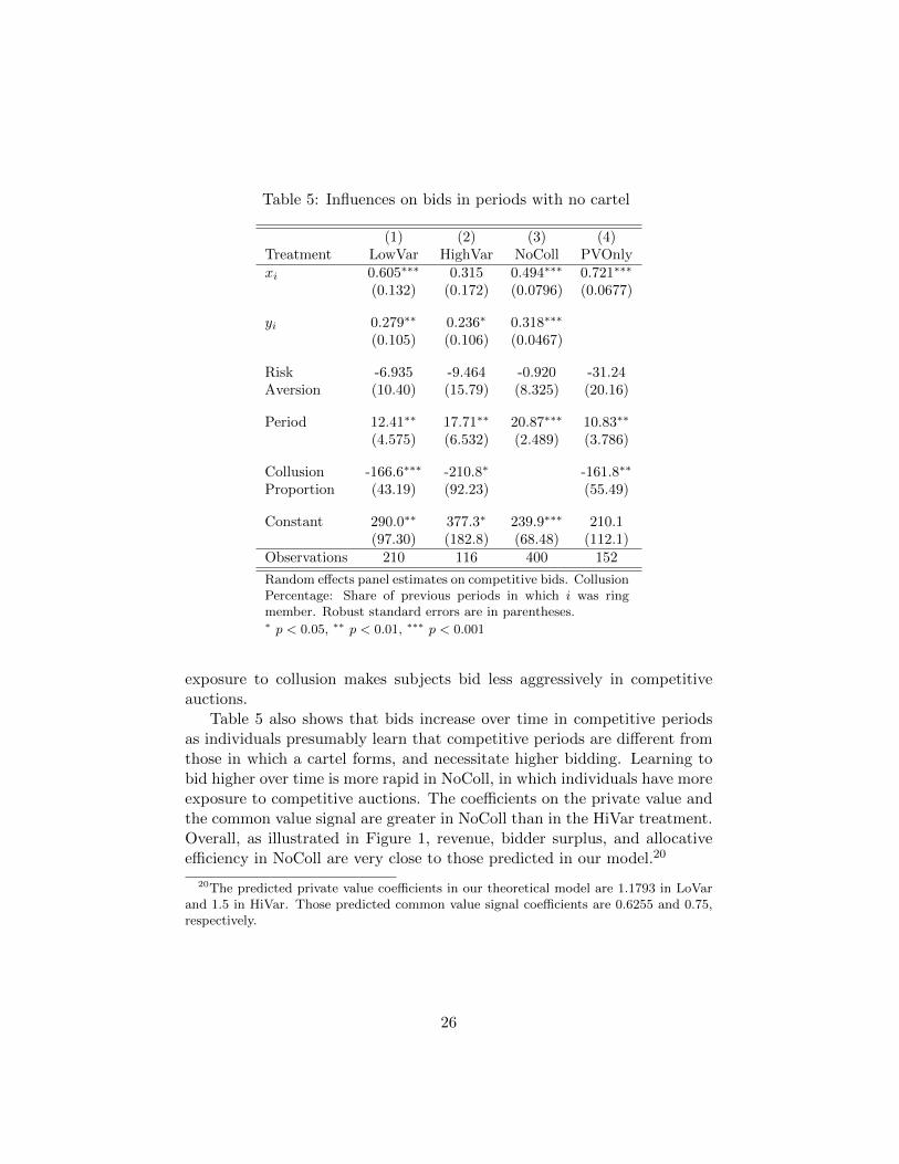
Table 5: Influences on bids in periods with no cartel

(1) (2) (3) (4)Treatment LowVar HighVar NoColl PVOnlyxi 0.605∗∗∗ 0.315 0.494∗∗∗ 0.721∗∗∗

(0.132) (0.172) (0.0796) (0.0677)

yi 0.279∗∗ 0.236∗ 0.318∗∗∗

(0.105) (0.106) (0.0467)

Risk -6.935 -9.464 -0.920 -31.24Aversion (10.40) (15.79) (8.325) (20.16)

Period 12.41∗∗ 17.71∗∗ 20.87∗∗∗ 10.83∗∗

(4.575) (6.532) (2.489) (3.786)

Collusion -166.6∗∗∗ -210.8∗ -161.8∗∗

Proportion (43.19) (92.23) (55.49)

Constant 290.0∗∗ 377.3∗ 239.9∗∗∗ 210.1(97.30) (182.8) (68.48) (112.1)

Observations 210 116 400 152

Random effects panel estimates on competitive bids. CollusionPercentage: Share of previous periods in which i was ringmember. Robust standard errors are in parentheses.∗ p < 0.05, ∗∗ p < 0.01, ∗∗∗ p < 0.001

exposure to collusion makes subjects bid less aggressively in competitiveauctions.

Table 5 also shows that bids increase over time in competitive periodsas individuals presumably learn that competitive periods are different fromthose in which a cartel forms, and necessitate higher bidding. Learning tobid higher over time is more rapid in NoColl, in which individuals have moreexposure to competitive auctions. The coefficients on the private value andthe common value signal are greater in NoColl than in the HiVar treatment.Overall, as illustrated in Figure 1, revenue, bidder surplus, and allocativeefficiency in NoColl are very close to those predicted in our model.20

20The predicted private value coefficients in our theoretical model are 1.1793 in LoVarand 1.5 in HiVar. Those predicted common value signal coefficients are 0.6255 and 0.75,respectively.

26

0.0

02

.004

.006

Density

0 100 200 300 400Absolute Difference PV

Absolute Difference PV, Collusion

Absolute Difference PV, Competition

kernel = epanechnikov, bandwidth = 21.6894

Kernel density estimate

0.0

01

.002

.003

.004

.005

Density

0 200 400 600 800Belief Error CV

Absolute Difference CV, Collusion

Absolute Difference CV, Competition

kernel = epanechnikov, bandwidth = 33.2784

Kernel density estimate

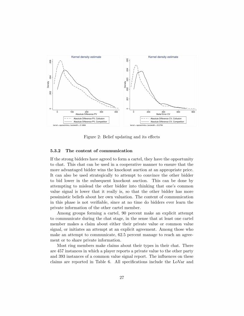
Figure 2: Belief updating and its effects

5.3.2 The content of communication

If the strong bidders have agreed to form a cartel, they have the opportunityto chat. This chat can be used in a cooperative manner to ensure that themore advantaged bidder wins the knockout auction at an appropriate price.It can also be used strategically to attempt to convince the other bidderto bid lower in the subsequent knockout auction. This can be done byattempting to mislead the other bidder into thinking that one’s commonvalue signal is lower that it really is, so that the other bidder has morepessimistic beliefs about her own valuation. The content of communicationin this phase is not verifiable, since at no time do bidders ever learn theprivate information of the other cartel member.

Among groups forming a cartel, 90 percent make an explicit attemptto communicate during the chat stage, in the sense that at least one cartelmember makes a claim about either their private value or common valuesignal, or initiates an attempt at an explicit agreement. Among those whomake an attempt to communicate, 62.5 percent manage to reach an agree-ment or to share private information.

Most ring members make claims about their types in their chat. Thereare 457 instances in which a player reports a private value to the other partyand 393 instances of a common value signal report. The influences on theseclaims are reported in Table 6. All specifications include the LoVar and

27

HiVar treatments.The coefficients of common value signals are highly significant determi-

nants of the reports of these variables. The other variables in the regressionare not significant, with the exception of the common value variance andone’s own earnings in the preceding period. Estimates on the constant termand on yi show that subjects underreport their CV signals. This is con-sistent with strategic communication, since beliefs about the other bidder’scommon value signals are a component of their beliefs about their own valu-ation. A lower assessment of the other bidder’s common value signal wouldprompt a bidder to bid lower. Risk aversion and earnings in the previousperiod are also significant factors, but the estimated effects associated withthese variables are small.

The coefficients of the private value are positive but low, and they areonly significant at 10 percent level. Furthermore, the intercept is substan-tially above 0. This lack of truthful reporting of private values may reflectattempts to behave strategically in the belief that keeping one’s private valueinformation to oneself can be beneficial.

5.3.3 Beliefs

As we have seen, there is widespread misreporting of both private valuesand common value signals during the communication stage. The subse-quent belief elicitation stage allows us to measure whether these reportswere believed.

The two graphs in Figure 2 show Epanechnikov kernel density estimatesof the distribution of the reported and actual distributions of the PV and CVsignals, in both collusive and competitive periods, for the pooled data fromthe LoVar and HiVar treatments. The left graph depicts the private value,while the right one depicts common value beliefs. The distributions illustratethe absolute differences between elicited beliefs and the corresponding actualvalues. The mean difference between actual values and elicited beliefs is125.4 and 93.4 under competition and collusion for the PV, and 157.7 vs125.7 for the CV signal. The Kolmogorov-Smirnov test rejects that thedistributions are identical at significance level 0.1 percent. That is, theperformance of subjects in the belief elicitation stage is improved if theyengage in collusion and explicitly communicate, indicating that there is aleakage of private information during the communication stage.21

21The payoffs in the belief elicitation stage also indicate that collusion improved theaccuracy of beliefs. The mean payoff in the belief elicitation stage was 44.91 under com-petition and 88.37 under collusion.

28

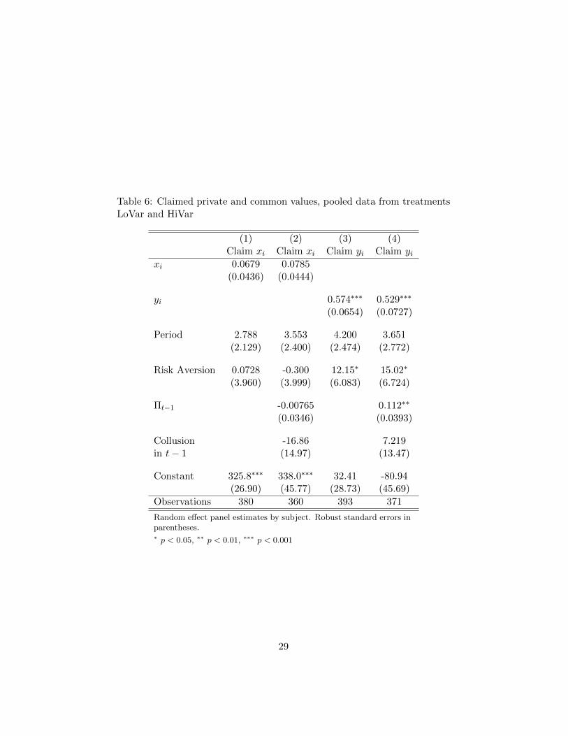
Table 6: Claimed private and common values, pooled data from treatmentsLoVar and HiVar

(1) (2) (3) (4)Claim xi Claim xi Claim yi Claim yi

xi 0.0679 0.0785(0.0436) (0.0444)

yi 0.574∗∗∗ 0.529∗∗∗

(0.0654) (0.0727)

Period 2.788 3.553 4.200 3.651(2.129) (2.400) (2.474) (2.772)

Risk Aversion 0.0728 -0.300 12.15∗ 15.02∗

(3.960) (3.999) (6.083) (6.724)

Πt−1 -0.00765 0.112∗∗

(0.0346) (0.0393)

Collusion -16.86 7.219in t− 1 (14.97) (13.47)

Constant 325.8∗∗∗ 338.0∗∗∗ 32.41 -80.94(26.90) (45.77) (28.73) (45.69)

Observations 380 360 393 371

Random effect panel estimates by subject. Robust standard errors inparentheses.∗ p < 0.05, ∗∗ p < 0.01, ∗∗∗ p < 0.001

29

0.0

01

.002

.003

.004

0 100 200 300 400y_ j

Actual CV, LoVar Belief CV, LoVar

0.0

005

.001

.0015

.002

0 200 400 600 800y_ j

Actual CV, HiVar Belief CV, HiVar

0.0

01

.002

.003

.004

0 100 200 300 400y_ j

Claim CV, LoVar Belief CV, LoVar0

.0005

.001

.0015

.002

0 200 400 600 800y_ j

Claim CV, HiVar Belief CV, HiVar

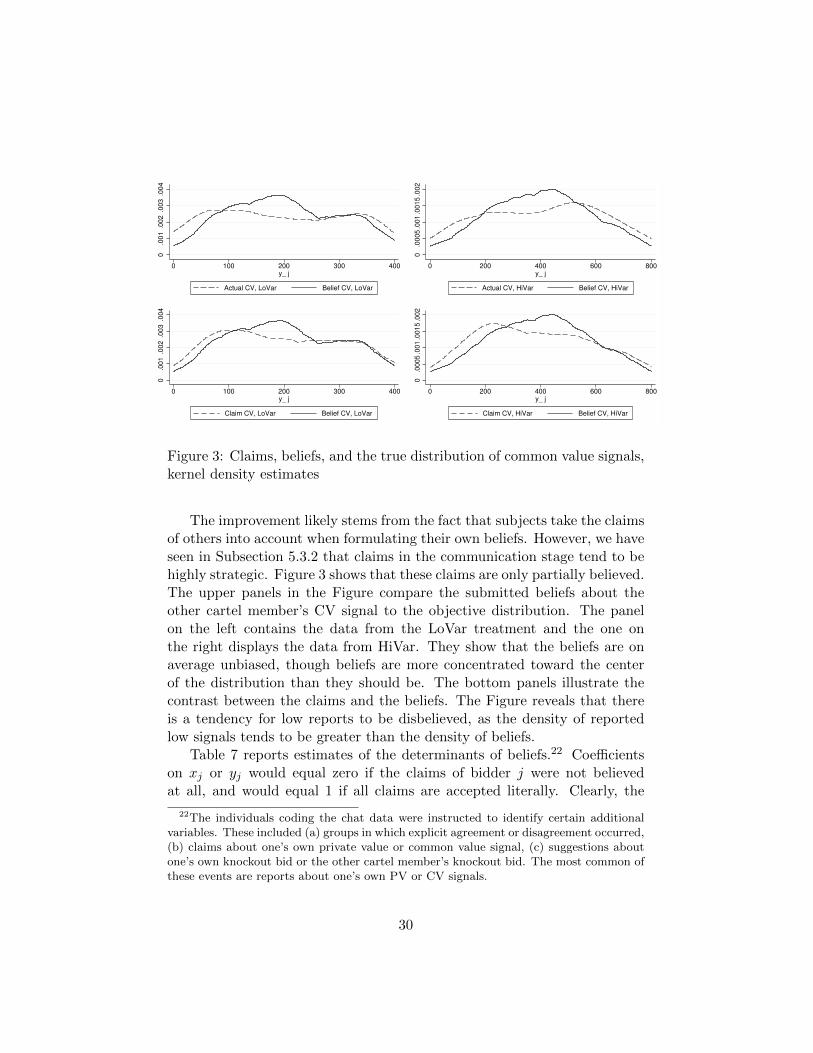
Figure 3: Claims, beliefs, and the true distribution of common value signals,kernel density estimates

The improvement likely stems from the fact that subjects take the claimsof others into account when formulating their own beliefs. However, we haveseen in Subsection 5.3.2 that claims in the communication stage tend to behighly strategic. Figure 3 shows that these claims are only partially believed.The upper panels in the Figure compare the submitted beliefs about theother cartel member’s CV signal to the objective distribution. The panelon the left contains the data from the LoVar treatment and the one onthe right displays the data from HiVar. They show that the beliefs are onaverage unbiased, though beliefs are more concentrated toward the centerof the distribution than they should be. The bottom panels illustrate thecontrast between the claims and the beliefs. The Figure reveals that thereis a tendency for low reports to be disbelieved, as the density of reportedlow signals tends to be greater than the density of beliefs.

Table 7 reports estimates of the determinants of beliefs.22 Coefficientson xj or yj would equal zero if the claims of bidder j were not believedat all, and would equal 1 if all claims are accepted literally. Clearly, the

22The individuals coding the chat data were instructed to identify certain additionalvariables. These included (a) groups in which explicit agreement or disagreement occurred,(b) claims about one’s own private value or common value signal, (c) suggestions aboutone’s own knockout bid or the other cartel member’s knockout bid. The most common ofthese events are reports about one’s own PV or CV signals.

30

Table 7: Belief updating and its effect

(1) (2) (3) (4) (5)Belief xj Belief yj Belief xj Belief yj Belief xj

Treatment LoVar LoVar HiVar HiVar PVOnlyClaim xj 0.780∗∗∗ 0.605∗∗∗ 0.656∗∗∗

(0.0683) (0.0675) (0.173)

Claim yj 0.771∗∗∗ 0.649∗∗∗

(0.0425) (0.0875)

Period 1.685 0.393 -5.019 -2.154 -8.835∗∗

(1.970) (1.566) (2.939) (4.333) (2.732)

Risk Aversion 1.464 -2.556 5.315 11.86 5.186(1.982) (3.285) (6.976) (11.74) (4.698)

Constant 63.04 55.80∗∗ 148.9∗∗∗ 104.8∗∗ 234.4∗

(33.58) (18.81) (34.67) (36.62) (93.26)Observations 240 238 139 143 60

Random effect panel estimates by subject. Standard errors in parentheses∗ p < 0.05, ∗∗ p < 0.01, ∗∗∗ p < 0.001

coefficients of the communicated private values and common value signalson beliefs about these variables are significant at conventional levels for alltreatments. This shows that claims are at least partially believed. However,the coefficients are also all significantly less than one, which means that theyare not taken at face value.

5.3.4 The knockout auction

Our model makes predictions of the bids in the knockout auction and wecompare the observed data to these predictions. Correlates of knockout bidsare identified in the random effects regressions reported in Table 8. The es-timates show that knockout bids are increasing in one’s own private value,which is predicted in our model and associated with greater efficiency. How-ever, the value of the constant is positive, and the coefficients on PV and CVsignal are significantly lower than the model’s prediction. This means thatthe bidding function is flatter in its key arguments than predicted.23 Beliefs

23We have run alternative specifications including the own private and common value asregressors. The estimates are not significant except for the coefficient of yi on the beliefsabout yj , and only in LoVar. The estimated coefficient is low, 0.16.

31

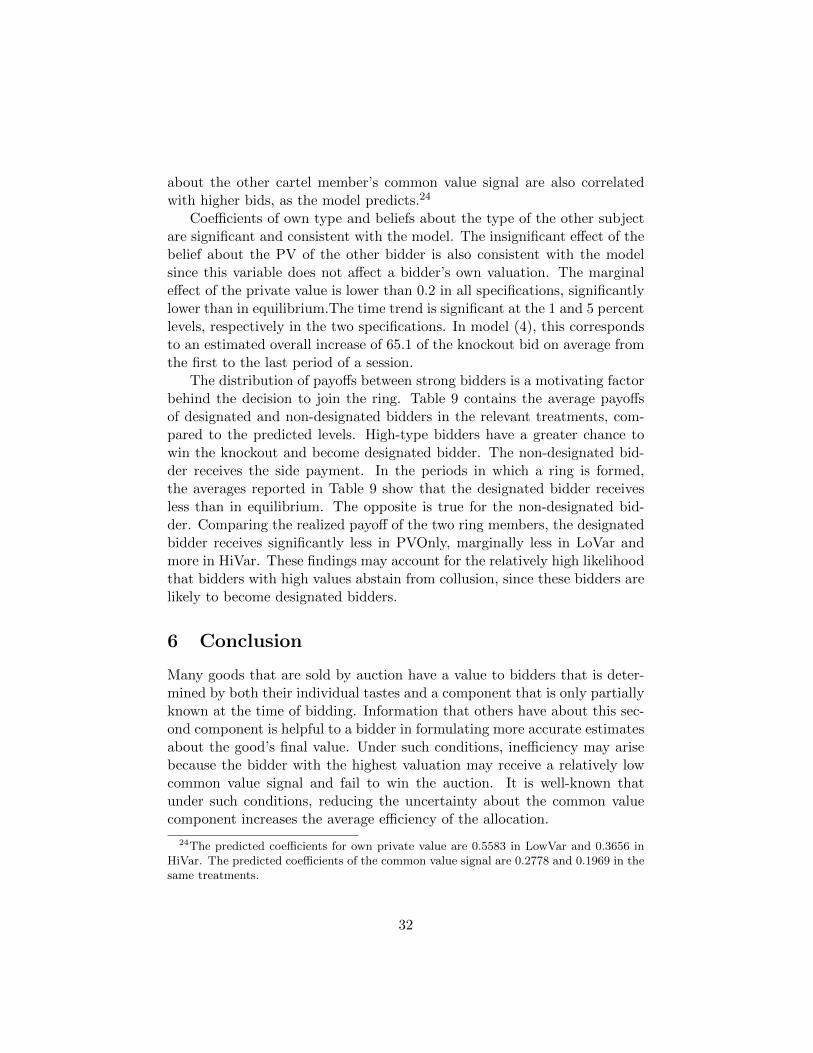
about the other cartel member’s common value signal are also correlatedwith higher bids, as the model predicts.24

Coefficients of own type and beliefs about the type of the other subjectare significant and consistent with the model. The insignificant effect of thebelief about the PV of the other bidder is also consistent with the modelsince this variable does not affect a bidder’s own valuation. The marginaleffect of the private value is lower than 0.2 in all specifications, significantlylower than in equilibrium.The time trend is significant at the 1 and 5 percentlevels, respectively in the two specifications. In model (4), this correspondsto an estimated overall increase of 65.1 of the knockout bid on average fromthe first to the last period of a session.

The distribution of payoffs between strong bidders is a motivating factorbehind the decision to join the ring. Table 9 contains the average payoffsof designated and non-designated bidders in the relevant treatments, com-pared to the predicted levels. High-type bidders have a greater chance towin the knockout and become designated bidder. The non-designated bid-der receives the side payment. In the periods in which a ring is formed,the averages reported in Table 9 show that the designated bidder receivesless than in equilibrium. The opposite is true for the non-designated bid-der. Comparing the realized payoff of the two ring members, the designatedbidder receives significantly less in PVOnly, marginally less in LoVar andmore in HiVar. These findings may account for the relatively high likelihoodthat bidders with high values abstain from collusion, since these bidders arelikely to become designated bidders.

6 Conclusion

Many goods that are sold by auction have a value to bidders that is deter-mined by both their individual tastes and a component that is only partiallyknown at the time of bidding. Information that others have about this sec-ond component is helpful to a bidder in formulating more accurate estimatesabout the good’s final value. Under such conditions, inefficiency may arisebecause the bidder with the highest valuation may receive a relatively lowcommon value signal and fail to win the auction. It is well-known thatunder such conditions, reducing the uncertainty about the common valuecomponent increases the average efficiency of the allocation.

24The predicted coefficients for own private value are 0.5583 in LowVar and 0.3656 inHiVar. The predicted coefficients of the common value signal are 0.2778 and 0.1969 in thesame treatments.

32

Table 8: The effect of private information and beliefs on knockout bids

(1) (2) (3)LoVar HiVar PVOnly

xi 0.166∗ 0.169∗∗ 0.269∗

(0.0721) (0.0593) (0.112)

yi 0.0801 0.0462(0.0465) (0.0275)

Belief 0.0658 0.0503 -0.0119xj (0.0565) (0.0899) (0.138)

Belief 0.174∗∗ 0.0445yj (0.0647) (0.0479)

Period 2.507 12.64∗∗∗ 0.630(3.258) (2.937) (4.494)

Risk Aversion -6.037 4.563 9.033(7.762) (8.046) (18.61)

Constant 114.0 77.88 86.79(59.57) (52.64) (166.9)

Observations 332 254 156

Random effect panel estimates by subject.

Standard errors in parentheses.∗ p < 0.05, ∗∗ p < 0.01, ∗∗∗ p < 0.001

Table 9: Mean payoffs of the designated and non-designated bidders withinthe bidding rings

Designated Bidder Non-designated BidderActual Prediction Actual Prediction

PVOnly 119.43 288.14 204.12 129.60LoVar 168.72 306.49 180.16 118.43HiVar 294.13 482.51 229.65 143.04

33

One way to decrease the uncertainty about the common value componentis to let bidders collude. Information can be exchanged, bidders can transferside payments to each other, and a designated bidder can be chosen in amanner that increases efficiency. The theoretical model that we proposedescribes how this would work. The model describes a situation in whichtwo bidders have an opportunity to form a cartel and jointly bid against aweak bidder. A knockout auction determines which bidder is designated tobid and the side payment the other bidder receives.

Our model makes three main predictions. The first is that efficiencyincreases in the presence of a cartel. The second is that an increase in com-mon value uncertainty decreases the efficiency of the final allocation undera cartel. The third is that all potential bidders join the cartel, regardless oftheir private information.

We report an experiment designed to test the three predictions. We findthat a large majority of individuals do choose to join a cartel. The principalinaccuracy is a tendency for bidders with higher valuations to sometimesforego cartel participation, and it appears rational to do so in light of therelatively small payoffs of designated cartel bidders. Comparison of theLoVar and HiVar treatments shows that inefficiency is greater in HiVar,when the common value signal variance is greater, than in LoVar. Thesetwo results are consistent with the model. However, we observe that thelevel of inefficiency is actually greater when a cartel forms than when it isnot, indicating that this prediction of the model is not borne out. It appearsthat frictions in the collusion process, which involves more stages in whichinefficiency can potentially appear, account for this pattern.

An additional treatment, NoColl, is identical to HiVar except that col-lusion is not permitted. The NoColl treatment generates higher prices thanthe HiVar treatment, even in those trials of HiVar when a cartel was notformed. This pattern suggests that prior experience with the low prices in acartel has a carryover effect that leads to less aggressive bidding and higherpayoffs to bidders in subsequent competitive auctions.

The PVOnly treatment, in which bidder valuations have only a privatevalue component leads to less cartel formation than the LoVar and HiVartreatments. This may reflect a recognition on the part of bidders that acartel can be helpful to members in learning about their own valuations,a motivation that does not exist in PVOnly. Indeed, in PVOnly, collusionlowers efficiency quite substantially.25

25While the PVOnly treatment can be viewed as a special case in which our modelcan be applied, it is a setting in which a key element of the model, the common value

34

The experiment also identifies a number of consistent behavioral pat-terns beyond our model’s predictions. Communication between colludingbidders tends to be strategic, and bidders underreport their common valuesignals. These reports tend to be greeted with skepticism and only partiallybelieved. Nevertheless, reported private values and signals are increasingin their true values, resulting in a significant improvement of beliefs undercollusion. In the knockout auction, there is some heterogeneity in behaviorbetween bidders, perhaps reflecting a preference of some bidders to be des-ignated bidders in the main auction and a preference of some others to leavethe bidding to the other party. Thus, while it is possible that efficiency isincreased by the information exchange within the cartel, it is offset by inef-ficiencies created by the system of allocation of the role of designated bidderfor the main auction, and of the side payment to the other cartel member.Our design had features that would enhance the efficiency of the cartel. Thedesignated bidder was allocated endogenously and communication allowedfor pooling of private information. Despite this, we found that collusionincreases inefficiency.

We are unable to find evidence that allowing collusion can increase inef-ficiency. Instead, we find that there is a negative effect on efficiency. Allow-ing collusion hurts sellers, by depressing bids and revenue, even in auctionswhere a cartel does not actually form. While bidders gain additional surplus,this remains below predicted levels. Thus, we find no compelling evidencearguing in favor of permitting bidders to collude.

component, does not exist.

35

Appendices

The appendices are intended as online supplementary material. There arefour appendices. The first consists of the Instructions for the experiment(Appendix A). The second contains the control questionnaire (AppendixB). Appendix C reproduce the instructions for the second part of the ex-periment, in which risk preferences were elicited. The instructions for theindividuals coding the chat data are given in Appendix D.

Appendix A Instructions

The following session is an experiment in decision-making. The instructionsare written here and read out loud before we start. If you follow them anddepending on your decisions, you can earn a considerable amount of money,which will be transferred to you after the end of the experiment. The amountof payment you receive depends on your decisions, on the decisions of others,and on chance. Your ID number for the experiment is the computer ID youcan find next to you. The entire experiment is anonymous, so we will usethis ID to call you when the payments are paid out at the end.

The currency used in the experiment is Coin. All amounts will be ex-pressed in terms of Coin. The cash payment at the end of the experimentwill be given to you in Euro. The conversion rate is 100 Coins to 1 Euro.Once the experiment has started, no one is allowed to talk to anybody otherthan the experimenter. If you have a question please raise your hand and wewill go to your place. During the entire experiment, please remain seated.

The experiment consists of two parts. Your final payment will be thesum of your payments for these two parts. In the following you will learnthe details of the first part.

Auction experiment

The experiment will consist of a sequence of 11 rounds in which you partic-ipate in an auction where you can bid for an object X. Of these 11 rounds,the first one will be for practice and the other 10 might count towards yourpayment. At the beginning of each round, you will begin with an endow-ment of 800 Coins. A round’s outcome is independent from other rounds.So, your payment in any given round will not be affected by your or others’decisions in other rounds.

In each round, you are randomly paired with an anonymous other par-ticipant in the room. That is, we will never tell you the identity of the

36

participant you are paired with. Neither will we tell the other participantyour identity. When a new round starts, new pairs are formed, and everyonein the room has equal chance to be paired up with you.

Before the auction takes place, you are allowed to communicate with theother bidder in your group and to make an agreement. The following listsummarizes the timing of each round; you can read the details below.

1. Redemption value: In the first stage you learn values Ayou and Byou

affecting your redemption value. If you acquire a unit of X, you canredeem it for Coin. The amount of Coins that a unit of X gives youis called your redemption value.

2. Decision: You are asked about your willingness to cooperate with theother bidder in your group. If you both reply ’Yes’, you continue withthe Chat stage. In other words, no agreement is made unless both ofyou wants to make one.

3. Chat : If you and the other bidder decide to cooperate, you can chatand make an agreement.

4. Guessing game: You are asked to guess the redemption value of theother bidder in the group.

5. Agreement : If you and the other bidder decide to cooperate, and makean agreement, you can read the details of this agreement on yourscreen.

6. Auction: The auction takes place.

7. Results: You can read the final results of the round.

Redemption value

In the auction you are bidding for a good called X with the other bidderand a computerized bidder.

If you acquire the good in the auction, you redeem it for your redemptionvalue. The redemption value can be different for bidders in the same auction.Your redemption value will be denoted by Ryou. Now we explain how is itcalculated.

You and the other human bidder are given two random numbers pri-vately, denoted by A and B. A is between 200 and 600 Coins, B is between0 and 400 Coins. Your and the other bidder‘s numbers are denoted by Ayou,

37

Aother, Byou and Bother. These numbers are integers, and all possible num-bers have an equal chance of being drawn. All numbers are independentlydrawn.

Your redemption value is calculated from these numbers. Before theauction, you only know Ayou and Byou but you do not know Aother andBother. Similarly, the other player knows Aother and Bother, but does notknow Ayouand Byou.

Your redemption value is calculated from Ayou, Byou and Bother as:

Ryou = Ayou +Byou + Bother

2

Similarly redemption value of the other human bidder is:

Rother = Aother +Byou + Bother

2

That is, the first component is different for you and the other human bidder.The second one,

Byou+Bother

2 is the same, and determined by Byou, which onlyyou can see, and Bother, which only the other bidder can see.

Decision

Before the auction takes place, you are allowed to chat with the other humanplayer, and you can make an agreement. Participation at the decision stagedepends on your and the other player‘s decision. A question appears in eachround and your answer only affects that particular round.

The following question appears on your screen. ’Do you wish to coop-erate with the other bidder in your group?’ If you both reply ’Yes’, youcontinue with the chat stage. If at least one of you replies ’No’, you proceedto the guessing game and to the auction. In other words, no agreement ismade unless both of you wants to make one.

Chat

If you both replied ’Yes’ at the decision stage, a chat box and a proposalbox appear. In the chat box you send a message by pressing the [Enter]button on your keyboard. You have 90 seconds available for chat. Duringthat time, you are allowed to talk about the numbers you observed (Ayou,Byou) and you can agree on a strategy for the remainder of the round. Theother player in your group is able to see the message that you send, butnothing more. So he or she cannot see on the screen whether you write thetruth.

38

You are free to discuss whatever you like except: Do not use any wordsor phrase which helps to identify you. Only communicate in English. Incase you violate these rules, you must leave the experiment and you receiveno payment.

You leave the chat by making a proposal to other player in your groupnext to the text ’Please, make your proposal!’. By clicking OK, you leave thechat. The purpose of this part of the round is to decide who will participatein the auction and how much compensation the other participant should getfor not participating.

In the bracket ’Make your proposal’, you are allowed to type a number,which is not bigger than your endowment. The one making the higherproposal has to pay the lower of the two amounts (in other words, thesecond highest proposal) to the other player, which is deducted from herendowment. If the numbers are equal, one of you is chosen with equalchance to do so. If you receive a payment, you do not participate in theauction, and your bid will be automatically 0. The payoff of this round is:

payoff = endowment + smaller proposal

The other player participates in the auction with the computerized bidderwith:

balance = endowment− smaller proposal

The proposal part can make two things possible for your group. First,you can share information during chat. Second, you can decide who shouldparticipate in the auction. If an agreement is made, one of you who payscan have only one opposing bidder, the computer.

Guessing game

The next stage is a guessing game in which everyone participates, eventhe pairs who decided not to cooperate. On your screen you can see twoquestions and two brackets in which you are asked to write numbers. Theseare ’How much do you think Aother is?’ and ’How much do you think Bother

is?’In the brackets, you are asked to guess the numbers of the other player

in your group. The available information to you is what you can have readin the instructions and what the other player writes to you during the chat.There is an extra payment for guessing right. The closer your guesses are tothe actual number, the more you earn. This amount is not added to your

39

balance in this round, but it is counted at the end of the experiment if theround is the one that counts. The maximum you can earn with guessing is200 Coins, with a perfect guess.

For example, if Aother = 550, Bother = 200 and your guesses are 550and 200, your payoff is 200 Coins for the guessing game. Your payoff isdetermined using the difference between Aother, Bother and your guesses.Suppose your guesses are 630 and 280 it means your guess was more faraway from Aother, you get 72 Coins. The least you can earn is 0 Coin.

Agreement

Before the auction, a new stage appears, which provides you informationabout the outcome of the proposals. This can only be seen by pairs whodecided to cooperate. You can see your new balance and whether you areallowed to participate in the auction.

Auction

The auction has two or three participants, depending on whether you andthe other player in your group made an agreement. The auction has similarrules as the proposal part. That is, you are required to make your bids atthe same time. The winner of the auction is the one making the highest bid.In case of a tie, the winner is chosen randomly among the ones with thehighest bids. The amount paid is the second highest bid submitted. In theauction stage, you are allowed to submit an integer number in the bracket’Please, make your bid’, that is at least 0.

The computer submits a number, that is between 0 and 500 Coins.The highest bidder receives the unit of X being sold and earns his or

her redemption value for it. If you win, your redemption value equals Ryou.Other participants, who do not win any X, do not pay any Coin and do notreceive any X, so their earnings for the period equal their balance. Thus, ifyou win, your payoff is:

yourpayoff = yourbalance− second highest bid +Ryou

= yourbalance− second highest bid +Ayou +Byou + Bother

2

Let us see an example. Suppose you have cooperated with the other player inyour group and you have given 150 Coins. Your new balance is 800− 150 =650 Coins. Suppose your values are Ayou = 500 and Byou = 100. You decideto bid 650. The computer bids 200. The other bidder does not participate,

40

so the second highest bid is 200 Coins. You win the auction, pay 200 Coins,and receive your redemption value. In order to calculate your redemptionvalue, you also need to know Bother. The only way you can learn it beforethe auction is by participating in the Chat round. Even in that case, youcan only see what the other human bidder writes, we do not show you theactual Bother.

Suppose Bother = 300. So, you redemption value is Ryou = 500 +300+100

2 = 500+200 = 700. So, your payoff of this round is 650+700−200 =1150 Coins. If someone does not win the auction, his resulting payoff ispayoff = balance. So, the other player receives 800 + 150 = 950 Coins,the sum of the endowment and the amount he or she has received by theagreement.

Results

After all bidders have submitted their bids, the outcome of the auction isannounced. You can read whether you have won, all the submitted bidsand your earnings for the round. You can see this screen even if you didnot participate in the auction. The process is repeated 11 times. The firstround is only practice, whereas one of the remaining 10 counts towards yourpayment. At the beginning of the first round which could count, we ask youto type in your seat number. You can find this number on the separatingwall, and it is between 1-24. We need this in order to make the paymentsat the end of the session.

Your payoff and end of session

After the second part of the experiment, you will receive your payments incash. The amount you receive for the first part of the experiment is yourpayoff from a random round, including the payment of the guessing game ofthe same random round. After the 11 rounds of the auction game, you willparticipate in a second part of the experiment. Your earnings in the secondpart will be added to your final payment.

After the two parts, payments are made anonymously and individually.Please remain seated until we call you.

41

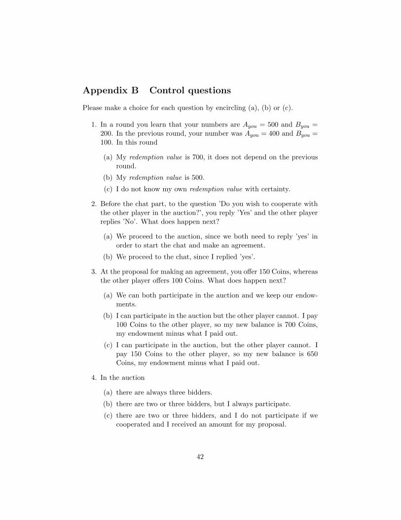
Appendix B Control questions

Please make a choice for each question by encircling (a), (b) or (c).

1. In a round you learn that your numbers are Ayou = 500 and Byou =200. In the previous round, your number was Ayou = 400 and Byou =100. In this round

(a) My redemption value is 700, it does not depend on the previousround.

(b) My redemption value is 500.

(c) I do not know my own redemption value with certainty.

2. Before the chat part, to the question ’Do you wish to cooperate withthe other player in the auction?’, you reply ’Yes’ and the other playerreplies ’No’. What does happen next?

(a) We proceed to the auction, since we both need to reply ’yes’ inorder to start the chat and make an agreement.

(b) We proceed to the chat, since I replied ’yes’.

3. At the proposal for making an agreement, you offer 150 Coins, whereasthe other player offers 100 Coins. What does happen next?

(a) We can both participate in the auction and we keep our endow-ments.

(b) I can participate in the auction but the other player cannot. I pay100 Coins to the other player, so my new balance is 700 Coins,my endowment minus what I paid out.

(c) I can participate in the auction, but the other player cannot. Ipay 150 Coins to the other player, so my new balance is 650Coins, my endowment minus what I paid out.

4. In the auction

(a) there are always three bidders.

(b) there are two or three bidders, but I always participate.

(c) there are two or three bidders, and I do not participate if wecooperated and I received an amount for my proposal.

42

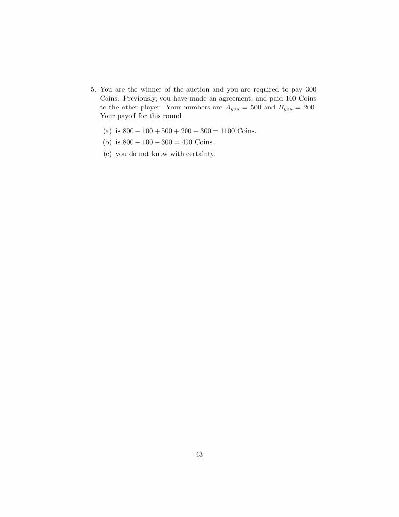
5. You are the winner of the auction and you are required to pay 300Coins. Previously, you have made an agreement, and paid 100 Coinsto the other player. Your numbers are Ayou = 500 and Byou = 200.Your payoff for this round

(a) is 800− 100 + 500 + 200− 300 = 1100 Coins.

(b) is 800− 100− 300 = 400 Coins.

(c) you do not know with certainty.

43

Appendix C Instruction HL protocol

In this part of the experiment you will be making choices between twolotteries, such as those represented as ”Option A” and “Option B” below.The money prizes are determined by the computer equivalent of throwinga ten-sided die. Each outcome, 1, 2, 3, 4, 5, 6, 7, 8, 9, 10, is equally likely.If you choose Option A in the decision shown below, you will have a 1 in10 chance of earning 500 Coins and a 9 in 10 chance of earning 400 Coins.Similarly, Option B offers a 1 in 10 chance of earning 960 Coins and a 9 in10 chance of earning 25 Coins.Decision 1:

Option A: 500 Coins if the die is 1 and 400 Coins if the die is 2 - 10.Option B: 960 Coins if the die is 1 and 25 Coins if the die is 2 - 10.

Each box of the decision table contains a pair of choices between Option Aand Option B. You make your choice by clicking on the “A” or “B“ buttonson the bottom. Only one option in each box can be selected, and you maychange your decision as you wish before you submit it.Even though you will make ten decisions, only one of these will end up beingused. The selection of the one to be used depends on the “throw of the die”,that is, it is determined by the computer’s random number generator. Nodecision is any more likely to be used than any other, and you will notknow in advance which one will be selected, so please think about each onecarefully.For example, suppose that you make all ten decisions and the roll of the dieis 9, then your choice, A or B, for decision 9 would be used and the otherdecisions would not be used.After the random die throw determines the decision box that will be used, asecond random number is drawn that determines the earnings for the optionyou chose for that box. In Decision 9 below, for example, a throw of 1, 2,3, 4, 5, 6, 7, 8, or 9 will result in the higher payoff for the option you chose,and a throw of 10 will result in the lower payoff.Decision 9:

Option A: 500 Coins if the die is 1-9 and 400 Coins if the die is 10Option B: 960 Coins if the die is 1-9 and 25 Coins if the die is 10

For decision 10, the random die throw will not be needed, since the choiceis between amounts of money that are fixed: 500 Coins for Option A and960 Coins for Option B.Your earnings in this part of the experiment will be added to your finalpayoff.

44

Appendix D Instructions chat coding

The following task is part of an experiment in decision-making. The in-structions are written here. If you follow them, you can earn a considerableamount of money, which will be transferred to you after completion of thetask. The amount of payment is fixed, 70 EUR. The content of all attachedfiles is confidential. You are not allowed to share it with anybody other thanthe experimenter. If you have a question, please contact us.

The instructions for the coding follow. Attached you can find a MS Excelfile with two spreadsheets, chat and data. Your task is to read the content ofchat and fill in the content of data. You can do this job anytime before thedeadline of December 17, at 17:00. At that point, the spreadsheet must becomplete. After delivering the completed file, you will receive your paymentby bank transfer, which will be sent to your account.

Chat

Spreadsheet chat contains observations from an anonymous economic exper-iment. The entries are chat messages and identification values. The meaningof each column is explained below. This database records the chat messagesof participants in experimental sessions.

• Period: This refers to the round in which the chat has taken place.There were 11 rounds, numbered between 0 and 10. Note that notevery participant had a chat in every round.

• Text: This is a chat message.

• Group: Code number of the group. A group consists of two partici-pants in a Period.

• Time: The time the message was sent.

• ID: identification number of the participant used (only) in the experi-ment.

In spreadsheet chat, the entries are ordered such that you can read aconversation between two participants easily. For example, rows 2, 3 and 4contain a conversation between subjects 102 and 105 in round 0, with chatmessages in chronological order. Note that not all participants participatedin chat for all periods. In all chats there were exactly two participants, butit is possible that only one of them has chat entries.

45

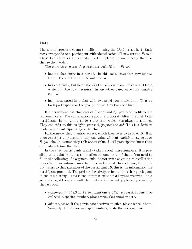
Data

The second spreadsheet must be filled in using the Chat spreadsheet. Eachrow corresponds to a participant with identification ID in a certain Period.These two variables are already filled in, please do not modify them orchange their order.

There are three cases. A participant with ID in a Period

• has no chat entry in a period. In this case, leave that row empty.Never delete entries for ID and Period.

• has chat entry, but he or she was the only one communicating. Pleasewrite 1 in the row onesided. In any other case, leave this variableempty.

• has participated in a chat with two-sided communication. That is,both participants of the group have sent at least one line.

If a participant has chat entries (case 2 and 3), you need to fill in theremaining cells. The conversation is about a proposal. After this chat, bothparticipants in the group made a proposal, which was always a number.They can refer to this as offer, proposal, payment or bid. This is a decisionmade by the participants after the chat.

Furthermore, they mention values, which they refer to as A or B. If ina conversation they mention only one value without explicitly saying A orB, you should assume they talk about value A. All participants knew theirown values before the chat.

In the chat, participants mainly talked about these numbers. It is pos-sible, that a chat contains no mention of some or all of them. You need tofill in the following. As a general rule, do not write anything in a cell if therespective information cannot be found in the chat. In each case, the prefixown refers to chat messages of the participant ID, this is the information theparticipant provided. The prefix other always refers to the other participantin the same group. This is the information the participant received. As ageneral rule, if there are multiple numbers for one entry, please type in onlythe last one.

• ownproposal : If ID in Period mentions a offer, proposal, payment orbid with a specific number, please write that number here.

• otherproposal : If the participant receives an offer, please write it here.Similarly, if there are multiple numbers, write the last one here.

46

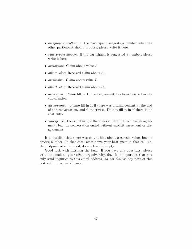
• ownproposaltoother : If the participant suggests a number what theother participant should propose, please write it here.

• otherproposaltoown: If the participant is suggested a number, pleasewrite it here.

• ownavalue: Claim about value A.

• otheravalue: Received claim about A.

• ownbvalue: Claim about value B.

• otherbvalue: Received claim about B.

• agreement : Please fill in 1, if an agreement has been reached in theconversation.

• disagreement : Please fill in 1, if there was a disagreement at the endof the conversation, and 0 otherwise. Do not fill it in if there is nochat entry.

• noresponse: Please fill in 1, if there was an attempt to make an agree-ment, but the conversation ended without explicit agreement or dis-agreement.

It is possible that there was only a hint about a certain value, but noprecise number. In that case, write down your best guess in that cell, i.e.the midpoint of an interval, do not leave it empty.

Good luck with finishing the task. If you have any questions, pleasewrite an email to g.seres@tilburguniversity.edu. It is important that youonly send inquiries to this email address, do not discuss any part of thistask with other participants.

47

References

Agranov, M., and L. Yariv (2016): “Collusion through Communicationin Auctions,” California Institute of Technology.

Apesteguia, J., M. Dufwenberg, and R. Selten (2007): “Blowing thewhistle,” Economic Theory, 31(1), 143–166.

Armantier, O., C. A. Holt, and C. R. Plott (2013): “A Procure-ment Auction for Toxic Assets with Asymmetric Information,” AmericanEconomic Journal: Microeconomics, 5(4), 142–162.

Armantier, O., and N. Treich (2013): “Eliciting beliefs: Proper scoringrules, incentives, stakes and hedging,” European Economic Review, 62,17–40.

Bigoni, M., S.-O. Fridolfsson, C. Le Coq, and G. Spagnolo (2015):“Trust, leniency, and deterrence,” Journal of Law, Economics, and Orga-nization, 31(4), 663–689.

Boone, J., R. Chen, J. K. Goeree, and A. Polydoro (2009): “Riskyprocurement with an insider bidder,” Experimental Economics, 12(4),417–436.

Brier, G. W. (1950): “Verification of forecasts expressed in terms of prob-ability,” Monthly Weather Review, 78(1), 1–3.

Coppinger, V. M., V. L. Smith, and J. A. Titus (1980): “Incentives andbehavior in English, Dutch and sealed-bid auctions,” Economic Inquiry,18(1), 1–22.

Cox, J. C., V. L. Smith, and J. M. Walker (1982): “Auction markettheory of heterogeneous bidders,” Economics Letters, 9(4), 319–325.

Fischbacher, U. (2007): “z-Tree: Zurich toolbox for ready-made economicexperiments,” Experimental Economics, 10(2), 171–178.

Goeree, J., and T. Offerman (2002): “Efficiency in auctions with pri-vate and common values: An experimental study,” American EconomicReview, 92(3), 625–643.

(2003): “Competitive bidding in auctions with private and commonvalues,” Economic Journal, 113(489), 598–613.

48

Groenewegen, J. (1994): “About double organized markets: issues ofcompetition and cooperation. The Dutch construction cartel: an illustra-tion,” Journal of Economic Issues, 28(3), 901–908.

Hinloopen, J., and S. Onderstal (2014): “Going once, going twice,reported! Cartel activity and the effectiveness of antitrust policies inexperimental auctions,” European Economic Review, 70, 317–336.

Hinloopen, J., and A. R. Soetevent (2014): “Exploitation and inducedtacit collusion: a classroom experiment of corporate leniency programs,”in The Analysis of Competition Policy and Sectoral Regulation, pp. 193–212.

Holt, C. A., and S. K. Laury (2002): “Risk aversion and incentiveeffects,” American Economic Review, 92(5), 1644–1655.

Hu, A., T. Offerman, and S. Onderstal (2011): “Fighting collusion inauctions: an experimental investigation,” International Journal of Indus-trial Organization, 29(1), 84–96.

Jehiel, P., and B. Moldovanu (2001): “Efficient design with interdepen-dent valuations,” Econometrica, 69(5), 1237–1259.

Li, J., Y. Xue, and W. Wu (2013): “Partnership dissolution and propri-etary information,” Social Choice and Welfare, 40(2), 495–527.

Llorente-Saguer, A., and R. Zultan (2014): “Auction mechanismsand bidder collusion: Bribes, signals and selection,” Working Paper, MaxPlanck Institute for Research on Collective Goods.

Mailath, G. J., and P. Zemsky (1991): “Collusion in second price auc-tions with heterogeneous bidders,” Games and Economic Behavior, 3(4),467–486.

Marshall, R. C., and L. M. Marx (2007): “Bidder collusion,” Journalof Economic Theory, 133(1), 374–402.

McAfee, R. P., and J. McMillan (1987): “Auctions and bidding,” Jour-nal of Economic Literature, 25(2), 699–738.

Milgrom, P. R., and R. J. Weber (1982): “A Theory of Auctions andCompetitive Bidding,” Econometrica, 50(5), 1089–1122.

Parlementaire Enquetecommissie Bouwnijverheid (2003):“Enquete bouwnijverheid,” Tweede Kamer der Staten-Generaal.

49

Selten, R. (1998): “Axiomatic characterization of the quadratic scoringrule,” Experimental Economics, 1(1), 43–62.

Sonnemans, J., and T. Offerman (2001): “Is the Quadratic ScoringRule really incentive compatible?,” Working paper CREED, University ofAmsterdam.

Vickrey, W. (1961): “Counterspeculation, auctions, and competitivesealed tenders,” The Journal of Finance, 16(1), 8–37.

50