the dynamics of adaboost: cyclic behavior and convergence...
TRANSCRIPT
Journal of Machine Learning Research 0 (0) 0 Submitted 0; Published 0
The Dynamics of AdaBoost: Cyclic Behavior and
Convergence of Margins
Cynthia Rudin [email protected], [email protected]
Program in Applied and Computational MathematicsFine HallWashington RoadPrinceton University Princeton, NJ 08544-1000, USA
Ingrid Daubechies [email protected]
Program in Applied and Computational MathematicsFine HallWashington RoadPrinceton University Princeton, NJ 08544-1000, USA
Robert E. Schapire [email protected]
Princeton University, Department of Computer Science
35 Olden St., Princeton, NJ 08544, USA
Editor: JMLR
Abstract
In order to study the convergence properties of the AdaBoost algorithm, we reduceAdaBoost to a nonlinear iterated map and study the evolution of its weight vectors. Thisdynamical systems approach allows us to understand AdaBoost’s convergence propertiescompletely in certain cases; for these cases we find stable cycles, allowing us to explicitlysolve for AdaBoost’s output.
Using this unusual technique, we are able to show that AdaBoost does not always con-verge to a maximum margin combined classifier, answering an open question. In addition,we show that “non-optimal” AdaBoost (where the weak learning algorithm does not neces-sarily choose the best weak classifier at each iteration) may fail to converge to a maximummargin classifier, even if “optimal” AdaBoost produces a maximum margin. Also, we showthat if AdaBoost cycles, it cycles among “support vectors”, i.e., examples that achieve thesame smallest margin.
Keywords: boosting, AdaBoost, dynamics, convergence, margins
1. Introduction
Boosting algorithms are currently among the most popular and most successful algorithmsfor pattern recognition tasks (such as text classification). AdaBoost [7] was the first practicalboosting algorithm, and due to its success, a number of similar boosting algorithms havesince been introduced (see Schapire’s review paper [22] for an introduction, or the reviewpaper of Meir and Ratsch [13]). Boosting algorithms are designed to construct a “strong”classifier using only a training set and a “weak” learning algorithm. A “weak” classifierproduced by the weak learning algorithm has a probability of misclassification that is slightly
c©0 Cynthia Rudin, Ingrid Daubechies, Robert E. Schapire.
Rudin, Daubechies, Schapire
below 50%, i.e., each weak classifier is only required to perform slightly better than a randomguess. A “strong” classifier has a much smaller probability of error on test data. Hence,these algorithms “boost” the weak learning algorithm to achieve a stronger classifier. Inorder to exploit the weak learning algorithm’s advantage over random guessing, the datais reweighted (the relative importance of the training examples is changed) before runningthe weak learning algorithm at each iteration. That is, AdaBoost maintains a distribution(set of weights) over the training examples, and selects a weak classifier from the weaklearning algorithm at each iteration. Training examples that were misclassified by the weakclassifier at the current iteration then receive higher weights at the following iteration. Theend result is a final combined classifier, given by a thresholded linear combination of theweak classifiers.
AdaBoost does not often seem to suffer from overfitting, even after a large numberof iterations [2, 14]. This lack of overfitting has been explained to some extent by themargin theory [23]. The margin of a boosted classifier is a number between -1 and 1, thataccording to the margin theory, can be thought of as a confidence measure of a classifier’spredictive ability, or as a guarantee on the generalization performance. If the margin ofa classifier is large, then it tends to perform well on test data. If the margin is small,then the classifier tends not to perform so well. (The margin of a boosted classifier is alsocalled the minimum margin over training examples.) Although the empirical success of aboosting algorithm depends on many factors (e.g., the type of data and how noisy it is, thecapacity of the weak learning algorithm, the number of boosting iterations, regularization,entire margin distribution over the training examples), the margin theory does provide areasonable explanation (though not a complete explanation) of AdaBoost’s success, bothempirically and theoretically.
Since the margin tends to give a strong indication of a classifier’s performance in prac-tice, a natural goal is to find classifiers that achieve a maximum margin. Since the AdaBoostalgorithm was invented before the margin theory, the algorithm became popular due to itspractical success rather than for its theoretical success (its ability to achieve large mar-gins). Since AdaBoost was not specifically designed to maximize the margin, the questionremained whether in fact it does actually maximize the margin. The objective function thatAdaBoost minimizes (the exponential loss) is not related to the margin in the sense thatone can minimize the exponential loss while simultaneously achieving an arbitrarily bad(small) margin. Thus, AdaBoost does not, in fact, optimize a cost function of the margins(see also Wyner [24]). It was shown analytically that AdaBoost produces large margins,namely, Schapire et al. [23] showed that AdaBoost achieves at least half of the maximummargin, and Ratsch and Warmuth [16] have recently tightened this bound slightly. How-ever, because AdaBoost does not necessarily make progress towards increasing the marginat each iteration, the usual techniques for analyzing coordinate algorithms do not apply; forall the extensive theoretical and empirical study of AdaBoost prior to the present work, itremained unknown whether or not AdaBoost always achieves a maximum margin solution.
A number of other boosting algorithms emerged over the past few years that aim moreexplicitly to maximize the margin at each iteration, such as AdaBoost∗ [16], arc-gv [3],Coordinate Ascent Boosting and Approximate Coordinate Ascent Boosting [21, 20, 18], thelinear programming (LP) boosting algorithms including LP-AdaBoost [9] and LPBoost [5](also see ε-boosting [17]). However, AdaBoost is still used in practice, because it empirically
2

The Dynamics of AdaBoost
seems to produce maximum margin classifiers with low generalization error, is easy toprogram, and has the fastest convergence rate of the coordinate algorithms. In fact, undertightly controlled tests, it was shown empirically that the maximum margin algorithmsarc-gv and LP-AdaBoost tend to perform worse than AdaBoost [3, 9]. In the experimentsof Grove and Schuurmans [9], AdaBoost achieved margins that were almost as large, (butnot quite as large) as those of the LP algorithms when stopped after a large number ofiterations, yet achieved lower generalization error.
Another surprising result of empirical trials is that AdaBoost does seem to be convergingto maximum margin solutions asymptotically in the numerical experiments of Grove andSchuurmans [9] and Ratsch and Warmuth [16]. Grove and Schuurmans have questionedwhether AdaBoost is simply a “general, albeit very slow, LP solver”. If AdaBoost is simplya margin-maximization algorithm, then why are other algorithms that achieve the samemargin performing worse than AdaBoost? Is AdaBoost simply a fancy margin-maximizationalgorithm in disguise, or is it something more? As we will see, the answers are sometimesyes and sometimes no. So clearly the margins do not tell the whole story.
AdaBoost, as shown repeatedly [1, 8, 15, 6, 12], is actually a coordinate descent algo-rithm on a particular exponential loss function. However, minimizing this function in otherways does not necessarily achieve large margins; the process of coordinate descent must besomehow responsible. Hence, we look to AdaBoost’s dynamics to understand the processby which the margin is generated.
In this work, we took an unusual approach to this problem. We simplified AdaBoost toreveal a nonlinear iterated map for AdaBoost’s weight vector. This iterated map gives adirect relation between the weights at time t and the weights at time t+1, including renor-malization, and thus provides a much more concise mapping than the original algorithm.We then analyzed this dynamical system in specific cases. Using a small toolbox of tech-niques for analyzing dynamical systems, we were able to avoid the problem that progress(with respect to the margin) does not occur at every iteration. Instead, we measure progressanother way; namely, via the convergence towards limit cycles.
To explain this way of measuring progress more clearly, we have found that for somespecific cases, the weight vector of AdaBoost produces limit cycles that can be analyticallystated, and are stable. When stable limit cycles exist, the convergence of AdaBoost can beunderstood. Thus, we are able to provide the key to answering the question of AdaBoost’sconvergence to maximum margin solutions: a collection of examples in which AdaBoost’sconvergence can be completely understood.
Using a very low-dimensional example (8 × 8, i.e., 8 weak classifiers and 8 trainingexamples), we are able to show that AdaBoost does not always produce a maximum marginsolution, finally answering the open question.
There are two interesting cases governing the dynamics of AdaBoost: the case wherethe optimal weak classifiers are chosen at each iteration (the “optimal” case), and the casewhere permissible non-optimal weak classifiers may be chosen (the “non-optimal” case). Inthe optimal case (which is the case we usually consider), the weak learning algorithm isrequired to choose a weak classifier that has the largest edge at every iteration, where theedge measures the performance of the weak learning algorithm. In the non-optimal case,the weak learning algorithm may choose any weak classifier as long as its edge exceeds ρ,the maximum margin achievable by a combined classifier. This is a natural notion of non-
3

Rudin, Daubechies, Schapire
optimality for boosting, thus it provides a natural sense in which to measure robustness.Based on large scale experiments and a gap in theoretical bounds, Ratsch and Warmuth [16]conjectured that AdaBoost does not necessarily converge to a maximum margin classifierin the non-optimal case, i.e., that AdaBoost is not robust in this sense. In practice, theweak classifiers are generated by CART or another weak learning algorithm, implying thatthe choice need not always be optimal.
In Section 8, we show this conjecture to be true using a 4×5 example. That is, we showthat “non-optimal AdaBoost” (AdaBoost in the non-optimal case) may not converge to amaximum margin solution, even in cases where “optimal AdaBoost” does.
Empirically, we have found very interesting and remarkable cyclic dynamics in manydifferent low-dimensional cases (many more cases than the ones analyzed in this paper), forexample, those illustrated in Figure 6. In fact, we have empirically found that AdaBoostproduces cycles on randomly generated matrices – even on random matrices with hundredsof dimensions. On low-dimensional random matrices, cycles are almost always produced inour experiments. Thus, the story of AdaBoost’s dynamics does not end with the margins; itis important to study AdaBoost’s dynamics in more general cases where these cycles occurin order to understand its convergence properties.
To this extent, we prove that if AdaBoost cycles, it cycles only among a set of “supportvectors” that achieve the same smallest margin among training examples. In addition,we give sufficient conditions for AdaBoost to achieve a maximum margin solution whencycling occurs. We also show that AdaBoost treats identically classified examples as oneexample, in the sense we will describe in Section 6. In Section 10, we discuss a case in whichAdaBoost exhibits indications of chaotic behavior, namely sensitivity to initial conditions,and movement into and out of cyclic behavior.
We proceed as follows: in Section 2 we introduce some notation and state the AdaBoostalgorithm. Then in Section 3 we decouple the dynamics for AdaBoost in the binary caseso that we have a nonlinear iterated map. In Section 4, we analyze these dynamics for asimple case: the case where each weak classifier has one misclassified training example. Ina 3× 3 example, we find that the weight vectors always converge to one of two stable limitcycles, allowing us to calculate AdaBoost’s output vector directly. From this, we can provethe output of AdaBoost yields the best possible margin. We generalize this case to m × min Section 5. In Section 6 we discuss identically classified examples. Namely, we show thatthe weights on identically classified training examples can be shifted among these exampleswhile preserving the cycle; that is, manifolds of stable cycles can occur. For an extensionof the simple 3× 3 case, we show that manifolds of cycles exist and are stable. In Section 7we show that the training examples AdaBoost cycles upon are “support vectors” in thatthey all achieve the same margin. In the process, we provide a formula to directly calculatethe margin from the cycle parameters. We also give sufficient conditions for AdaBoost toproduce a maximum margin classifier when cycling occurs. Then in Section 8 we producean example to show non-robustness of AdaBoost in the non-optimal case. In Section 9,we produce the example discussed above to show that AdaBoost may not converge to amaximum margin solution. And finally in Section 10, we provide a case for which AdaBoostexhibits indications of chaotic behavior.
4
The Dynamics of AdaBoost
2. Notation and Introduction to AdaBoost
The training set consists of examples with labels {(xi, yi)}i=1,...,m, where (xi, yi) ∈ X ×{−1, 1}. The space X never appears explicitly in our calculations. Let H = {h1, ..., hn} bethe set of all possible weak classifiers that can be produced by the weak learning algorithm,where hj : X → {1,−1}. We assume that if hj appears in H, then −hj also appears in H.Since our classifiers are binary, and since we restrict our attention to their behavior on afinite training set, we can assume the number of weak classifiers n is finite. We typicallythink of n as being very large, m ¿ n, which makes a gradient descent calculation imprac-tical because n, the number of dimensions, is too large; hence, AdaBoost uses coordinatedescent instead, where only one weak classifier is chosen at each iteration.
We define an m×n matrix M where Mij = yihj(xi), i.e., Mij = +1 if training examplei is classified correctly by weak classifier hj , and −1 otherwise. We assume that no columnof M has all +1’s, that is, no weak classifier can classify all the training examples correctly.(Otherwise the learning problem is trivial. In this case, AdaBoost will have an undefinedstep size.) Although M is too large to be explicitly constructed in practice, mathemati-cally, it acts as the only “input” to AdaBoost in this notation, containing all the necessaryinformation about the weak learning algorithm and training examples.
AdaBoost computes a set of coefficients over the weak classifiers. At iteration t, the(unnormalized) coefficient vector is denoted λt; i.e., the coefficient of weak classifier hj de-termined by AdaBoost at iteration t is λt,j . The final combined classifier that AdaBoostoutputs is fλtmax
given via λtmax/‖λtmax
‖1:
fλ =
∑nj=1 λjhj
‖λ‖1where ‖λ‖1 =
n∑
j=1
|λj |.
In the specific examples we provide, either hj or −hj remains unused over the course ofAdaBoost’s iterations, so all values of λt,j are non-negative. The margin of training examplei is defined by yifλ(xi). Informally, one can think of the margin of a training example as thedistance (by some measure) from the example to the decision boundary, {x : fλ(x) = 0}.
A boosting algorithm maintains a distribution, or set of weights, over the training ex-amples that is updated at each iteration t. This distribution is denoted dt ∈ ∆m, and dT
t
is its transpose. Here, ∆m denotes the simplex of m-dimensional vectors with non-negativeentries that sum to 1. At each iteration t, a weak classifier hjt
is selected by the weak learn-ing algorithm. The probability of error at iteration t, denoted d−, for the selected weakclassifier hjt
on the training examples (weighted by dt) is∑
{i:Mijt=−1} dt,i. Also, denote
d+ := 1− d−. Note that d+ and d− depend on t; although we have simplified the notation,the iteration number will be clear from the context. The edge of weak classifier jt at timet with respect to the training examples is (dT
t M)jt, which can be written as
(dTt M)jt
=∑
i:Mijt=1
dt,i −∑
i:Mijt=−1
dt,i = d+ − d− = 1 − 2d−.
Thus, a smaller edge indicates a higher probability of error. For the optimal case (thecase we usually consider), we will require the weak learning algorithm to give us the weak
5
Rudin, Daubechies, Schapire
classifier with the largest possible edge at each iteration,
jt ∈ argmaxj
(dTt M)j ,
i.e., jt is the weak classifier that performs the best on the training examples weighted by dt.For the non-optimal case (which we consider in Section 8), we only require a weak classifierwhose edge exceeds ρ, where ρ is the largest possible margin that can be attained for M,i.e.,
jt ∈ {j : (dTt M)j ≥ ρ}.
(The value ρ is defined formally below.) The edge for the chosen weak classifier jt atiteration t is denoted rt, i.e., rt = (dT
t M)jt. Note that d+ = (1+ rt)/2 and d− = (1− rt)/2.
The margin theory developed via a set of generalization bounds that are based on themargin distribution of the training examples [23, 10]. These bounds can be reformulated (ina slightly weaker form) in terms of the minimum margin, which was the focus of previouswork by Breiman [3], Grove and Schuurmans [9], and Ratsch and Warmuth [16]. Thus,these bounds suggest maximizing the minimum margin over training examples to achieve alow probability of error over test data. Hence, our goal is to find a normalized vector λ ∈ ∆n
that maximizes the minimum margin over training examples, mini (Mλ)i (or equivalentlymini yifλ(xi)). That is, we wish to find a vector
λ ∈ argmaxλ∈∆n
mini
(Mλ)i.
We call this minimum margin over training examples (i.e., mini(Mλ)i/‖λ‖1) the `1-marginor simply margin of classifier λ. Any training example that achieves this minimum marginwill be called a support vector. Due to the von Neumann Min-Max Theorem for 2-playerzero-sum games,
mind∈∆m
maxj
(dTM)j = maxλ∈∆n
mini
(Mλ)i.
That is, the minimum value of the edge (left hand side) corresponds to the maximum valueof the margin (i.e., the maximum value of the minimum margin over training examples,right hand side). We denote this value by ρ. One can think of ρ as measuring the worstperformance of the best combined classifier, mini(Mλ)i.
The “unrealizable” or “non-separable” case where ρ = 0 is fully understood [4]. For thiswork, we assume ρ > 0 and study the less understood “realizeable” or “separable” case.In both the non-separable and separable cases, AdaBoost converges to a minimizer of theempirical loss function
F (λ) :=m∑
i=1
e−(Mλ)i .
In the non-separable case, the dt’s converge to a fixed vector [4]. In the separable case,the dt’s cannot converge to a fixed vector, and the minimum value of F is 0, occurring as||λ||1 → ∞. It is important to appreciate that this tells us nothing about the value of themargin achieved by AdaBoost or any other procedure designed to minimize F . To see why,consider any λ ∈ ∆n such that (Mλ)i > 0 for all i (assuming we are in the separable caseso such a λ exists). Then lima→∞ aλ will produce a minimum value for F , but the original
6
The Dynamics of AdaBoost
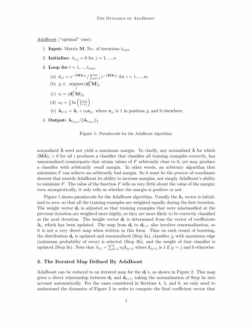
AdaBoost (“optimal” case):
1. Input: Matrix M, No. of iterations tmax
2. Initialize: λ1,j = 0 for j = 1, ..., n
3. Loop for t = 1, ..., tmax
(a) dt,i = e−(Mλt)i/∑m
i=1 e−(Mλt)i for i = 1, ..., m
(b) jt ∈ argmaxj
(dTt M)j
(c) rt = (dTt M)jt
(d) αt = 12 ln
(1+rt
1−rt
)
(e) λt+1 = λt + αtejt, where ejt
is 1 in position jt and 0 elsewhere.
4. Output: λtmax/‖λtmax
‖1
Figure 1: Pseudocode for the AdaBoost algorithm.
normalized λ need not yield a maximum margin. To clarify, any normalized λ for which(Mλ)i > 0 for all i produces a classifier that classifies all training examples correctly, hasunnormalized counterparts that attain values of F arbitrarily close to 0, yet may producea classifier with arbitrarily small margin. In other words, an arbitrary algorithm thatminimizes F can achieve an arbitrarily bad margin. So it must be the process of coordinatedescent that awards AdaBoost its ability to increase margins, not simply AdaBoost’s abilityto minimize F . The value of the function F tells us very little about the value of the margin;even asymptotically, it only tells us whether the margin is positive or not.
Figure 1 shows pseudocode for the AdaBoost algorithm. Usually the λ1 vector is initial-ized to zero, so that all the training examples are weighted equally during the first iteration.The weight vector dt is adjusted so that training examples that were misclassified at theprevious iteration are weighted more highly, so they are more likely to be correctly classifiedat the next iteration. The weight vector dt is determined from the vector of coefficientsλt, which has been updated. The map from dt to dt+1 also involves renormalization, soit is not a very direct map when written in this form. Thus on each round of boosting,the distribution dt is updated and renormalized (Step 3a), classifier jt with maximum edge(minimum probability of error) is selected (Step 3b), and the weight of that classifier isupdated (Step 3e). Note that λt,j =
∑tt=1 αt1jt=j where 1jt=j is 1 if jt = j and 0 otherwise.
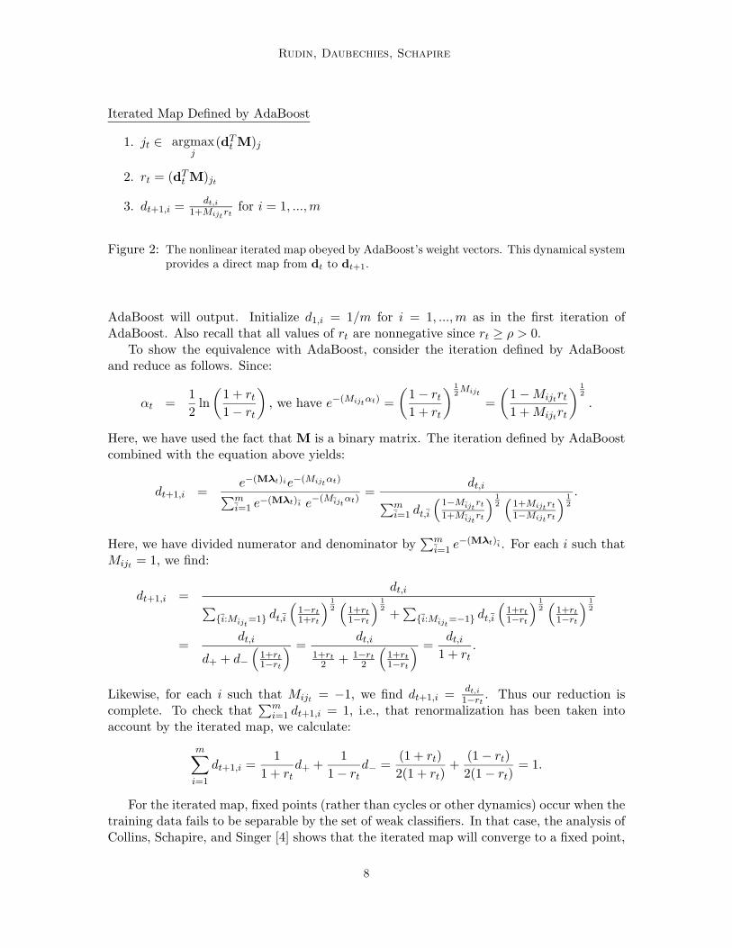
3. The Iterated Map Defined By AdaBoost
AdaBoost can be reduced to an iterated map for the dt’s, as shown in Figure 2. This mapgives a direct relationship between dt and dt+1, taking the normalization of Step 3a intoaccount automatically. For the cases considered in Sections 4, 5, and 6, we only need tounderstand the dynamics of Figure 2 in order to compute the final coefficient vector that
7
Rudin, Daubechies, Schapire
Iterated Map Defined by AdaBoost
1. jt ∈ argmaxj
(dTt M)j
2. rt = (dTt M)jt
3. dt+1,i =dt,i
1+Mijtrt
for i = 1, ..., m
Figure 2: The nonlinear iterated map obeyed by AdaBoost’s weight vectors. This dynamical systemprovides a direct map from dt to dt+1.
AdaBoost will output. Initialize d1,i = 1/m for i = 1, ..., m as in the first iteration ofAdaBoost. Also recall that all values of rt are nonnegative since rt ≥ ρ > 0.
To show the equivalence with AdaBoost, consider the iteration defined by AdaBoostand reduce as follows. Since:
αt =1
2ln
(1 + rt
1 − rt
), we have e−(Mijt
αt) =
(1 − rt
1 + rt
) 1
2Mijt
=
(1 − Mijt
rt
1 + Mijtrt
) 1
2
.
Here, we have used the fact that M is a binary matrix. The iteration defined by AdaBoostcombined with the equation above yields:
dt+1,i =e−(Mλt)ie−(Mijt
αt)
∑mi=1 e−(Mλt)i e−(Mijt
αt)=
dt,i
∑mi=1 dt,i
(1−Mijt
rt
1+Mijtrt
) 1
2
(1+Mijt
rt
1−Mijtrt
) 1
2
.
Here, we have divided numerator and denominator by∑m
i=1 e−(Mλt)i . For each i such thatMijt
= 1, we find:
dt+1,i =dt,i
∑{i:Mijt
=1} dt,i
(1−rt
1+rt
) 1
2
(1+rt
1−rt
) 1
2
+∑
{i:Mijt=−1} dt,i
(1+rt
1−rt
) 1
2
(1+rt
1−rt
) 1
2
=dt,i
d+ + d−(
1+rt
1−rt
) =dt,i
1+rt
2 + 1−rt
2
(1+rt
1−rt
) =dt,i
1 + rt
.
Likewise, for each i such that Mijt= −1, we find dt+1,i =
dt,i
1−rt. Thus our reduction is
complete. To check that∑m
i=1 dt+1,i = 1, i.e., that renormalization has been taken intoaccount by the iterated map, we calculate:
m∑
i=1
dt+1,i =1
1 + rt
d+ +1
1 − rt
d− =(1 + rt)
2(1 + rt)+
(1 − rt)
2(1 − rt)= 1.
For the iterated map, fixed points (rather than cycles or other dynamics) occur when thetraining data fails to be separable by the set of weak classifiers. In that case, the analysis ofCollins, Schapire, and Singer [4] shows that the iterated map will converge to a fixed point,
8

The Dynamics of AdaBoost
and that the λ′ts will asymptotically attain the minimum value of the convex function
F (λ) :=∑m
i=1 e−(Mλ)i , which is strictly positive in the non-separable case. Consider thepossibility of fixed points for the dt’s in the separable case ρ > 0. From our dynamics, wecan see that this is not possible, since rt ≥ ρ > 0 and for any i such that dt,i > 0,
dt+1,i =dt,i
(1 + Mi,jtrt)
6= dt,i.
Thus, we have shown that AdaBoost does not produce fixed points in the separable case.
4. The Dynamics of AdaBoost in the Simplest Case : The 3 × 3 Case
In this section, we will introduce a simple 3×3 input matrix (in fact, the simplest non-trivial matrix) and analyze the convergence of AdaBoost in this case, using the iteratedmap of Section 3. We will show that AdaBoost does produce a maximum margin solution,remarkably through convergence to one of two stable limit cycles. We extend this exampleto the m × m case in Section 5, where AdaBoost produces at least (m − 1)! stable limitcycles, each corresponding to a maximum margin solution. We will also extend this examplein Section 6 to include manifolds of cycles.
Consider the following input matrix
M =
−1 1 11 −1 11 1 −1
corresponding to the case where each classifier misclassifies one of three training examples.We could add columns to include the negated version of each weak classifier, but thosecolumns would never be chosen by AdaBoost, so they have been removed for simplicity.The value of the margin for the best combined classifier defined by M is 1/3. How willAdaBoost achieve this result? We will proceed step by step.
Assume we are in the optimal case, where jt ∈ argmaxj(dTt M)j . Consider the dynamical
system on the simplex ∆3 defined by our iterated map in Section 3. In the triangular regionwith vertices (0, 0, 1), (1
3 , 13 , 1
3), (0, 1, 0), jt will be 1 for Step 1 of the iterated map. That is,within this region, dt,1 < dt,2 and dt,1 < dt,3, so jt will be 1. Similarly, we have regions forjt = 2 and jt = 3 (see Figure 3(a)).
AdaBoost was designed to set the edge of the previous weak classifier to 0 at eachiteration, that is, dt+1 will always satisfy (dT
t+1M)jt= 0. To see this using the iterated
map,
(dTt+1M)jt
=∑
{i:Mijt=1}
dt,i1
1 + rt
−∑
{i:Mijt=−1}
dt,i1
1 − rt
= d+1
1 + rt
− d−1
1 − rt
=1 + rt
2
1
1 + rt
− 1 − rt
2
1
1 − rt
= 0. (1)
This implies that after the first iteration, the dt’s are restricted to:
{d : [(dTM)1 = 0]⋃
[(dTM)2 = 0]⋃
[(dTM)3 = 0]}.
9

Rudin, Daubechies, Schapire
Thus, it is sufficient for our dynamical system to be analyzed on the edges of a trianglewith vertices
(0, 1
2 , 12
),
(12 , 0, 1
2
),
(12 , 1
2 , 0)
(see Figure 3(b)). That is, within one iteration,the 2-dimensional map on the simplex ∆3 reduces to a 1-dimensional map on the edges ofthe triangle.
Consider the possibility of periodic cycles for the dt’s. If there are periodic cycles oflength T , then the following condition must hold for d
cyc1 , ...,dcyc
T in the cycle: For each i,either:
• dcyc1,i = 0, or
• ∏Tt=1(1 + Mijt
rcyct ) = 1,
where rcyct = (dcycT
t M)jt. (As usual, d
cyct
T:= (dcyc
t )T , superscript T denotes transpose.)The statement above follows directly from the reduced map iterated T times. In fact, thefirst condition dcyc
1,i = 0 implies dcyct,i = 0 for all t ∈ {1, ..., T}. We call the second condition
the cycle condition.
Consider the possibility of a periodic cycle of length 3, cycling through each weak clas-sifier once. For now, assume j1 = 1, j2 = 2, j3 = 3, but without loss of generality one canchoose j1 = 1, j2 = 3, j3 = 2, which yields another cycle. Assume dcyc
1,i > 0 for all i. Fromthe cycle condition,
1 = (1 + Mij1rcyc1 )(1 + Mij2r
cyc2 )(1 + Mij3r
cyc3 ) for i = 1, 2, and 3, i.e.,
1 = (1 − rcyc1 )(1 + rcyc
2 )(1 + rcyc3 ) for i = 1, (2)
1 = (1 + rcyc1 )(1 − rcyc
2 )(1 + rcyc3 ) for i = 2, (3)
1 = (1 + rcyc1 )(1 + rcyc
2 )(1 − rcyc3 ) for i = 3. (4)
From (2) and (3),
(1 − rcyc1 )(1 + rcyc
2 ) = (1 + rcyc1 )(1 − rcyc
2 ),
thus rcyc1 = rcyc
2 . Similarly, rcyc2 = rcyc
3 from (3) and (4), so rcyc1 = rcyc
2 = rcyc3 . Using either
(2), (3), or (4) to solve for r := rcyc1 = rcyc
2 = rcyc3 (taking positive roots since r > 0), we
find the value of the edge for every iteration in the cycle to be equal to the golden ratiominus one, i.e.,
r =
√5 − 1
2.
Now, let us solve for the weight vectors in the cycle, dcyc1 , d
cyc2 , and d
cyc3 . At t = 2, the edge
with respect to classifier 1 is 0. Again, it is required that each dcyct lies on the simplex ∆3.
(dcyc2
TM)1 = 0 and
3∑
i=1
dcyc2,i = 1, that is,
−dcyc2,1 + dcyc
2,2 + dcyc2,3 = 0 and dcyc
2,1 + dcyc2,2 + dcyc
2,3 = 1,
thus, dcyc2,1 =
1
2.
10

The Dynamics of AdaBoost
a) b)
t,2
t,1
j = 1
j = 2t
t j = 3t
1
1
d
d
1/3
1/3
t,1
t,2
(d M) =0
(d M) =0
(d M) =0
2
1
3t
t
tT
T
T
1
1
1/2
d
d
1/2
c1) c2) c3)
� � � � � � � � �� � � � � � � � �� � � � � � � � �� � � � � � � � �� � � � � � � � �� � � � � � � � �� � � � � � � � �� � � � � � � � �� � � � � � � � �� � � � � � � � �� � � � � � � � �� � � � � � � � �� � � � � � � � �� � � � � � � � �� � � � � � � � �� � � � � � � � �� � � � � � � � �� � � � � � � � �� � � � � � � � �� � � � � � � � �� � � � � � � � �� � � � � � � � �� � � � � � � � �� � � � � � � � �� � � � � � � � �� � � � � � � � �
� � � � � � � � �� � � � � � � � �� � � � � � � � �� � � � � � � � �� � � � � � � � �� � � � � � � � �� � � � � � � � �� � � � � � � � �� � � � � � � � �� � � � � � � � �� � � � � � � � �� � � � � � � � �� � � � � � � � �� � � � � � � � �� � � � � � � � �� � � � � � � � �� � � � � � � � �� � � � � � � � �� � � � � � � � �� � � � � � � � �� � � � � � � � �� � � � � � � � �� � � � � � � � �� � � � � � � � �� � � � � � � � �� � � � � � � � �
t,1
t,2
� � � � � � � � � � � �� � � � � � � � � � � �� � � � � � � � � � � �� � � � � � � � � � � �� � � � � � � � � � � �� � � � � � � � � � � �� � � � � � � � � � � �� � � � � � � � � � � �� � � � � � � � � � � �� � � � � � � � � � � �
� � � � � � � � � � � �� � � � � � � � � � � �� � � � � � � � � � � �� � � � � � � � � � � �� � � � � � � � � � � �� � � � � � � � � � � �� � � � � � � � � � � �� � � � � � � � � � � �� � � � � � � � � � � �� � � � � � � � � � � �
� � � � � � � � � � � �� � � � � � � � � � � �� � � � � � � � � � � �� � � � � � � � � � � �
� � � � � � � � � � � �� � � � � � � � � � � �� � � � � � � � � � � �� � � � � � � � � � � �
� � � � � � � � � � � �� � � � � � � � � � � �
� � � � � � � � � � �� � � � � � � � � � �� � � � � � � � � � �� � � � � � � � � � �� � � � � � � � � � �� � � � � � � � � � �� � � � � � � � � � �� � � � � � � � � � �
� � � � � � � � � �� � � � � � � � � �
� � � � � � � � �� � � � � � � � �� � � � � � � � �� � � � � � � � �� � � � � � � � �
� � � � � � �� � � � � � �� � � � � � �� � � � � � �� � � � � � �
� � � � � � �� � � � � � �� � � � � � �� � � � � � �
� � � � � � � � � � �� � � � � � � � � � �� � � � � � � � � � �� � � � � � � � � � �� � � � � � � � � � �� � � � � � � � � � �
� � � � � � � � � � �� � � � � � � � � � �� � � � � � � � � � �� � � � � � � � � � �� � � � � � � � � � �� � � � � � � � � � �
� � � � � � � � � � � �� � � � � � � � � � � �� � � � � � � � � � � �� � � � � � � � � � � �� � � � � � � � � � � �� � � � � � � � � � � �� � � � � � � � � � � �
� � � � � � � � � � � �� � � � � � � � � � � �� � � � � � � � � � � �� � � � � � � � � � � �� � � � � � � � � � � �� � � � � � � � � � � �� � � � � � � � � � � �
� � � � � � � � � � �� � � � � � � � � � �� � � � � � � � � � �� � � � � � � � � � �� � � � � � � � � � �� � � � � � � � � � �
� � � � � � � � � � �� � � � � � � � � � �� � � � � � � � � � �� � � � � � � � � � �� � � � � � � � � � �� � � � � � � � � � �
� � � � � � � � � � � �� � � � � � � � � � � �� � � � � � � � � � � �� � � � � � � � � � � �
1
1
1/2
d1/2
d
� � � � � � � � � � � � � � � � � � � � � � � � � �� � � � � � � � � � � � � � � � � � � � � � � � � �� � � � � � � � � � � � � � � � � � � � � � � � � �� � � � � � � � � � � � � � � � � � � � � � � � � �� � � � � � � � � � � � � � � � � � � � � � � � � �� � � � � � � � � � � � � � � � � � � � � � � � � �� � � � � � � � � � � � � � � � � � � � � � � � � �� � � � � � � � � � � � � � � � � � � � � � � � � �� � � � � � � � � � � � � � � � � � � � � � � � � �
� � � � � � � � � � � � � � � � � � � � � � � � � �� � � � � � � � � � � � � � � � � � � � � � � � � �� � � � � � � � � � � � � � � � � � � � � � � � � �� � � � � � � � � � � � � � � � � � � � � � � � � �� � � � � � � � � � � � � � � � � � � � � � � � � �� � � � � � � � � � � � � � � � � � � � � � � � � �� � � � � � � � � � � � � � � � � � � � � � � � � �� � � � � � � � � � � � � � � � � � � � � � � � � �� � � � � � � � � � � � � � � � � � � � � � � � � �
t,1
t,2
� � � �� � � �� � � �� � � �� � � �� � � �� � � �� � � �
� � � �� � � �� � � �� � � �� � � �� � � �� � � �� � � �
� � �� � �� � �� � �� � �� � �� � �� � �� � �� � �� � �� � �
� �� �� �� �� �� �� �� �� �� �� �� �
� � � � � � � � � � �� � � � � � � � � � �� � � � � � � � � � �� � � � � � � � � � �� � � � � � � � � � �� � � � � � � � � � �� � � � � � � � � � �� � � � � � � � � � �� � � � � � � � � � �� � � � � � � � � � �� � � � � � � � � � �� � � � � � � � � � �
� � � � � � � � � � �� � � � � � � � � � �� � � � � � � � � � �� � � � � � � � � � �� � � � � � � � � � �� � � � � � � � � � �� � � � � � � � � � �� � � � � � � � � � �� � � � � � � � � � �� � � � � � � � � � �� � � � � � � � � � �� � � � � � � � � � �
! ! ! ! ! ! ! ! !! ! ! ! ! ! ! ! !! ! ! ! ! ! ! ! !! ! ! ! ! ! ! ! !! ! ! ! ! ! ! ! !! ! ! ! ! ! ! ! !! ! ! ! ! ! ! ! !! ! ! ! ! ! ! ! !! ! ! ! ! ! ! ! !! ! ! ! ! ! ! ! !! ! ! ! ! ! ! ! !! ! ! ! ! ! ! ! !" " " " " " " " " " " " " "# # # # # # # # # # # # #
$ $ $$ $ $$ $ $$ $ $$ $ $$ $ $$ $ $$ $ $$ $ $$ $ $$ $ $
% %% %% %% %% %% %% %% %% %% %% %
& & && & && & && & && & && & && & && & && & && & &
' ' '' ' '' ' '' ' '' ' '' ' '' ' '' ' '' ' '' ' '
( ( ( ( (( ( ( ( (( ( ( ( (( ( ( ( (( ( ( ( (( ( ( ( (( ( ( ( (( ( ( ( (( ( ( ( (( ( ( ( (
) ) ) ) )) ) ) ) )) ) ) ) )) ) ) ) )) ) ) ) )) ) ) ) )) ) ) ) )) ) ) ) )) ) ) ) )) ) ) ) )
* * * * * * ** * * * * * ** * * * * * ** * * * * * ** * * * * * ** * * * * * ** * * * * * ** * * * * * ** * * * * * ** * * * * * ** * * * * * ** * * * * * *
+ + + + + + ++ + + + + + ++ + + + + + ++ + + + + + ++ + + + + + ++ + + + + + ++ + + + + + ++ + + + + + ++ + + + + + ++ + + + + + ++ + + + + + ++ + + + + + +
, , , , , , ,, , , , , , ,, , , , , , ,, , , , , , ,, , , , , , ,, , , , , , ,, , , , , , ,, , , , , , ,, , , , , , ,, , , , , , ,
- - - - - - -- - - - - - -- - - - - - -- - - - - - -- - - - - - -- - - - - - -- - - - - - -- - - - - - -- - - - - - -- - - - - - -
. . . .
. . . .
. . . .
. . . .
. . . .
. . . .
. . . .
. . . .
. . . .
. . . .
. . . .
/ / / // / / // / / // / / // / / // / / // / / // / / // / / // / / // / / /
000000000000
111111111111
1
1
1/2
d1/2
d
t,1
t,2
2 2 2 2 2 2 2 2 2 2 2 2 2 2 2 2 2 2 2 2 2 2 2 2 22 2 2 2 2 2 2 2 2 2 2 2 2 2 2 2 2 2 2 2 2 2 2 2 22 2 2 2 2 2 2 2 2 2 2 2 2 2 2 2 2 2 2 2 2 2 2 2 22 2 2 2 2 2 2 2 2 2 2 2 2 2 2 2 2 2 2 2 2 2 2 2 22 2 2 2 2 2 2 2 2 2 2 2 2 2 2 2 2 2 2 2 2 2 2 2 22 2 2 2 2 2 2 2 2 2 2 2 2 2 2 2 2 2 2 2 2 2 2 2 22 2 2 2 2 2 2 2 2 2 2 2 2 2 2 2 2 2 2 2 2 2 2 2 22 2 2 2 2 2 2 2 2 2 2 2 2 2 2 2 2 2 2 2 2 2 2 2 22 2 2 2 2 2 2 2 2 2 2 2 2 2 2 2 2 2 2 2 2 2 2 2 22 2 2 2 2 2 2 2 2 2 2 2 2 2 2 2 2 2 2 2 2 2 2 2 22 2 2 2 2 2 2 2 2 2 2 2 2 2 2 2 2 2 2 2 2 2 2 2 22 2 2 2 2 2 2 2 2 2 2 2 2 2 2 2 2 2 2 2 2 2 2 2 22 2 2 2 2 2 2 2 2 2 2 2 2 2 2 2 2 2 2 2 2 2 2 2 22 2 2 2 2 2 2 2 2 2 2 2 2 2 2 2 2 2 2 2 2 2 2 2 22 2 2 2 2 2 2 2 2 2 2 2 2 2 2 2 2 2 2 2 2 2 2 2 22 2 2 2 2 2 2 2 2 2 2 2 2 2 2 2 2 2 2 2 2 2 2 2 22 2 2 2 2 2 2 2 2 2 2 2 2 2 2 2 2 2 2 2 2 2 2 2 22 2 2 2 2 2 2 2 2 2 2 2 2 2 2 2 2 2 2 2 2 2 2 2 22 2 2 2 2 2 2 2 2 2 2 2 2 2 2 2 2 2 2 2 2 2 2 2 22 2 2 2 2 2 2 2 2 2 2 2 2 2 2 2 2 2 2 2 2 2 2 2 22 2 2 2 2 2 2 2 2 2 2 2 2 2 2 2 2 2 2 2 2 2 2 2 22 2 2 2 2 2 2 2 2 2 2 2 2 2 2 2 2 2 2 2 2 2 2 2 22 2 2 2 2 2 2 2 2 2 2 2 2 2 2 2 2 2 2 2 2 2 2 2 22 2 2 2 2 2 2 2 2 2 2 2 2 2 2 2 2 2 2 2 2 2 2 2 22 2 2 2 2 2 2 2 2 2 2 2 2 2 2 2 2 2 2 2 2 2 2 2 2
3 3 3 3 3 3 3 3 3 3 3 3 3 3 3 3 3 3 3 3 3 3 3 3 33 3 3 3 3 3 3 3 3 3 3 3 3 3 3 3 3 3 3 3 3 3 3 3 33 3 3 3 3 3 3 3 3 3 3 3 3 3 3 3 3 3 3 3 3 3 3 3 33 3 3 3 3 3 3 3 3 3 3 3 3 3 3 3 3 3 3 3 3 3 3 3 33 3 3 3 3 3 3 3 3 3 3 3 3 3 3 3 3 3 3 3 3 3 3 3 33 3 3 3 3 3 3 3 3 3 3 3 3 3 3 3 3 3 3 3 3 3 3 3 33 3 3 3 3 3 3 3 3 3 3 3 3 3 3 3 3 3 3 3 3 3 3 3 33 3 3 3 3 3 3 3 3 3 3 3 3 3 3 3 3 3 3 3 3 3 3 3 33 3 3 3 3 3 3 3 3 3 3 3 3 3 3 3 3 3 3 3 3 3 3 3 33 3 3 3 3 3 3 3 3 3 3 3 3 3 3 3 3 3 3 3 3 3 3 3 33 3 3 3 3 3 3 3 3 3 3 3 3 3 3 3 3 3 3 3 3 3 3 3 33 3 3 3 3 3 3 3 3 3 3 3 3 3 3 3 3 3 3 3 3 3 3 3 33 3 3 3 3 3 3 3 3 3 3 3 3 3 3 3 3 3 3 3 3 3 3 3 33 3 3 3 3 3 3 3 3 3 3 3 3 3 3 3 3 3 3 3 3 3 3 3 33 3 3 3 3 3 3 3 3 3 3 3 3 3 3 3 3 3 3 3 3 3 3 3 33 3 3 3 3 3 3 3 3 3 3 3 3 3 3 3 3 3 3 3 3 3 3 3 33 3 3 3 3 3 3 3 3 3 3 3 3 3 3 3 3 3 3 3 3 3 3 3 33 3 3 3 3 3 3 3 3 3 3 3 3 3 3 3 3 3 3 3 3 3 3 3 33 3 3 3 3 3 3 3 3 3 3 3 3 3 3 3 3 3 3 3 3 3 3 3 33 3 3 3 3 3 3 3 3 3 3 3 3 3 3 3 3 3 3 3 3 3 3 3 33 3 3 3 3 3 3 3 3 3 3 3 3 3 3 3 3 3 3 3 3 3 3 3 33 3 3 3 3 3 3 3 3 3 3 3 3 3 3 3 3 3 3 3 3 3 3 3 33 3 3 3 3 3 3 3 3 3 3 3 3 3 3 3 3 3 3 3 3 3 3 3 33 3 3 3 3 3 3 3 3 3 3 3 3 3 3 3 3 3 3 3 3 3 3 3 33 3 3 3 3 3 3 3 3 3 3 3 3 3 3 3 3 3 3 3 3 3 3 3 3
4 44 44 44 44 44 44 44 44 44 44 4
55555555555
6 66 66 66 66 66 66 66 66 6
7 77 77 77 77 77 77 77 7
8 8 88 8 88 8 88 8 88 8 88 8 88 8 88 8 8
9 9 99 9 99 9 99 9 99 9 99 9 99 9 99 9 9
: : :: : :: : :: : :: : :: : :
; ; ;; ; ;; ; ;; ; ;; ; ;; ; ;
< < < < << < < < << < < < << < < < << < < < << < < < << < < < <
= = = = == = = = == = = = == = = = == = = = == = = = == = = = =
> > > > >> > > > >> > > > >> > > > >> > > > >> > > > >
? ? ? ? ?? ? ? ? ?? ? ? ? ?? ? ? ? ?? ? ? ? ?? ? ? ? ?
@ @ @ @@ @ @ @@ @ @ @@ @ @ @
A A A AA A A AA A A AA A A A
B B B B B BB B B B B BB B B B B BB B B B B BB B B B B B
C C C C C CC C C C C CC C C C C CC C C C C CC C C C C C
D D D D D D DD D D D D D DD D D D D D D
E E E E E E EE E E E E E EE E E E E E E
F F F F F F F F F F FG G G G G G G G G G GH H H H H H H H H HH H H H H H H H H HH H H H H H H H H H
I I I I I I I I I II I I I I I I I I II I I I I I I I I I
1
1
1/2
d1/2
d
d) e)
t,1
t,2
1
1
1/2
d1/2
d
t,1
t,2
x
x
x
1
1
1/2
d1/2
d
Figure 3: (a) Regions of dt-space where classifiers jt = 1, 2, 3 will respectively be selected for Step1 of the iterated map of Figure 2. Since dt,3 = 1 − dt,2 − dt,1, this projection onto thefirst two coordinates dt,1 and dt,2 completely characterizes the map. (b) Regardless ofthe initial position d1, the weight vectors at all subsequent iterations d2, ...,dtmax
willbe restricted to lie on the edges of the inner triangle which is labelled. (c1) Withinone iteration, the triangular region where jt = 1 maps to the line {d : (dT M)1 = 0}.The arrows indicate where various points in the shaded region will map at the followingiteration. The other two regions have analogous dynamics as shown in (c2) and (c3). (d)There are six total subregions of the inner triangle (two for each of the three edges). Eachsubregion is mapped to the interior of another subregion as indicated by the arrows. (e)Coordinates for the two 3-cycles. The approximate positions d
cyc1 , d
cyc2 , and d
cyc3 for one
of the 3-cycles are denoted by a small ‘o’, the positions for the other cycle are denotedby a small ‘x’.
11
Rudin, Daubechies, Schapire
0.2 0.3 0.4 0.5
0.2
0.4
0.5
dt,1
d t,2
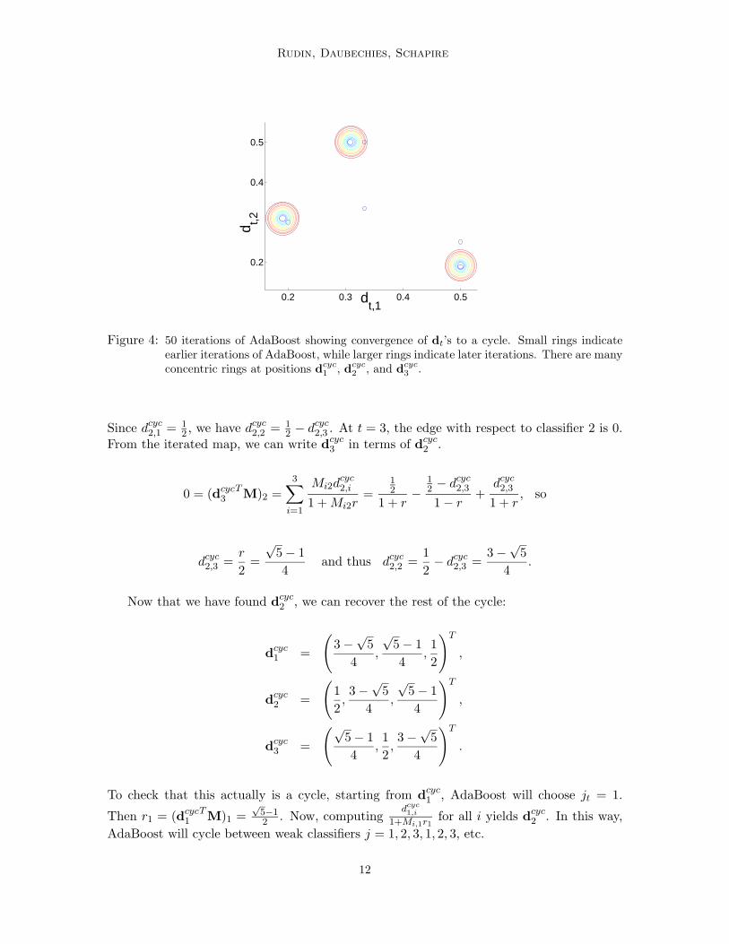
Figure 4: 50 iterations of AdaBoost showing convergence of dt’s to a cycle. Small rings indicateearlier iterations of AdaBoost, while larger rings indicate later iterations. There are manyconcentric rings at positions d
cyc1 , d
cyc2 , and d
cyc3 .
Since dcyc2,1 = 1
2 , we have dcyc2,2 = 1
2 − dcyc2,3 . At t = 3, the edge with respect to classifier 2 is 0.
From the iterated map, we can write dcyc3 in terms of d
cyc2 .
0 = (dcyc3
TM)2 =
3∑
i=1
Mi2dcyc2,i
1 + Mi2r=
12
1 + r−
12 − dcyc
2,3
1 − r+
dcyc2,3
1 + r, so
dcyc2,3 =
r
2=
√5 − 1
4and thus dcyc
2,2 =1
2− dcyc
2,3 =3 −
√5
4.
Now that we have found dcyc2 , we can recover the rest of the cycle:
dcyc1 =
(3 −
√5
4,
√5 − 1
4,1
2
)T
,
dcyc2 =
(1
2,3 −
√5
4,
√5 − 1
4
)T
,
dcyc3 =
(√5 − 1
4,1
2,3 −
√5
4
)T
.
To check that this actually is a cycle, starting from dcyc1 , AdaBoost will choose jt = 1.
Then r1 = (dcyc1
TM)1 =
√5−12 . Now, computing
dcyc1,i
1+Mi,1r1for all i yields d
cyc2 . In this way,
AdaBoost will cycle between weak classifiers j = 1, 2, 3, 1, 2, 3, etc.
12
The Dynamics of AdaBoost
The other 3-cycle can be determined similarly:
dcyc′
1 =
(3 −
√5
4,1
2,
√5 − 1
4
)T
,
dcyc′
2 =
(1
2,
√5 − 1
4,3 −
√5
4
)T
,
dcyc′
3 =
(√5 − 1
4,3 −
√5
4,1
2
)T
.
Since we always start from the initial condition d1 =(
13 , 1
3 , 13
)T, the initial choice of jt is
arbitrary; all three weak classifiers are within the argmax set in Step 1 of the iterated map.This arbitrary step, along with another arbitrary choice at the second iteration, determineswhich of the two cycles the algorithm will choose; as we will see, the algorithm must convergeto one of these two cycles.
To show that these cycles are globally stable, we will show that the map is a contractionfrom each subregion of the inner triangle into another subregion. We only need to con-sider the one-dimensional map defined on the edges of the inner triangle, since within oneiteration, every trajectory starting within the simplex ∆3 lands somewhere on the edgesof the inner triangle. The edges of the inner triangle consist of 6 subregions, as shown in
Figure 3(d). We will consider one subregion, the segment from(0, 1
2 , 12
)Tto
(14 , 1
2 , 14
)T, or
simply(x, 1
2 , 12 − x
)Twhere x ∈ (0, 1
4). (We choose not to deal with the endpoints since wewill show they are unstable; thus the dynamics never reach or converge to these points. Forthe first endpoint the map is not defined, and for the second, the map is ambiguous; notwell-defined.) For this subregion jt = 1, and the next iterate is:
(x
1 − (1 − 2x),
12
1 + (1 − 2x),
12 − x
1 + (1 − 2x)
)T
=
(1
2,
1
4(1 − x),1
2− 1
4(1 − x)
)T
.
To compare the length of the new interval with the length of the previous interval, we usethe fact that there is only one degree of freedom. A position on the previous interval canbe uniquely determined by its first component x ∈ (0, 1
4). A position on the new intervalcan be uniquely determined by its second component taking values 1
4(1−x) , where we still
have x ∈ (0, 14). The map
x 7→ 1
4(1 − x)
is a contraction. To see this, the slope of the map is 14(1−x)2
, taking values within the
interval (14 , 4
9). Thus the map is continuous and monotonic, with absolute slope strictly less
than 1. The next iterate will appear within the interval(
12 , 1
4 , 14
)Tto
(12 , 1
3 , 16
)T, which is
strictly contained within the subregion connecting(
12 , 1
4 , 14
)Twith
(12 , 1
2 , 0)T
. Thus, we havea contraction. A similar calculation can be performed for each of the subregions, showingthat each subregion maps monotonically to an area strictly within another subregion by acontraction map. Figure 3(d) illustrates the various mappings between subregions. After
13

Rudin, Daubechies, Schapire
a) b)
(0,.5,.5) (.5,.5,0) (.5,.0,.5) (0,.5,.5)(0,.5,.5)
(.5,.5,0)
(.5,.0,.5)
(0,.5,.5)
position along triangle
posi
tion
alon
g tr
iang
le
(0,.5,.5) (.5,.5,0) (.5,.0,.5) (0,.5,.5)(0,.5,.5)
(.5,.5,0)
(.5,0,.5)
(0,.5,.5)
position along triangle
posi
tion
alon
g tr
iang
le
Figure 5: (a) The iterated map on the unfolded triangle. Both axes give coordinates on the edgesof the inner triangle in Figure 3(b). The plot shows where dt+1 will be, given dt. (b)The map from (a) iterated twice, showing where dt+3 will be, given dt. For this “triplemap”, there are 6 stable fixed points, 3 for each cycle.
three iterations, each subregion maps by a monotonic contraction to a strict subset of itself.Thus, any fixed point of the three-iteration cycle must be the unique attracting fixed pointfor that subregion, and the domain of attraction for this point must be the whole subregion.In fact, there are six such fixed points, one for each subregion, three for each of the twocycles. The union of the domains of attraction for these fixed points is the whole triangle;every position d within the simplex ∆3 is within the domain of attraction of one of these3-cycles. Thus, these two cycles are globally stable.
Since the contraction is so strong at every iteration (as shown above, the absolute slopeof the map is much less than 1), the convergence to one of these two 3-cycles is veryfast. Figure 5(a) shows where each subregion of the “unfolded triangle” will map after thefirst iteration. The “unfolded triangle” is the interval obtained by traversing the triangleclockwise, starting and ending at
(0, 1
2 , 12
). Figure 5(b) illustrates that the absolute slope
of the second iteration of this map at the fixed points is much less than 1; the cycles arestrongly attracting.
The combined classifier that AdaBoost will output is:
λcombined =
(12 ln
(1+r
cyc1
1−rcyc1
), 1
2 ln(
1+rcyc2
1−rcyc2
), 1
2 ln(
1+rcyc3
1−rcyc3
))T
normalization constant=
(1
3,1
3,1
3
)T
,
and since mini(Mλcombined)i = 13 , we see that AdaBoost always produces a maximum
margin solution for this input matrix.
Thus, we have derived our first convergence proof for AdaBoost in a specific separablecase. We have shown that at least in some cases, AdaBoost is in fact a margin-maximizingalgorithm. We summarize this first main result.
Theorem 1 For the 3 × 3 matrix M:
14
The Dynamics of AdaBoost
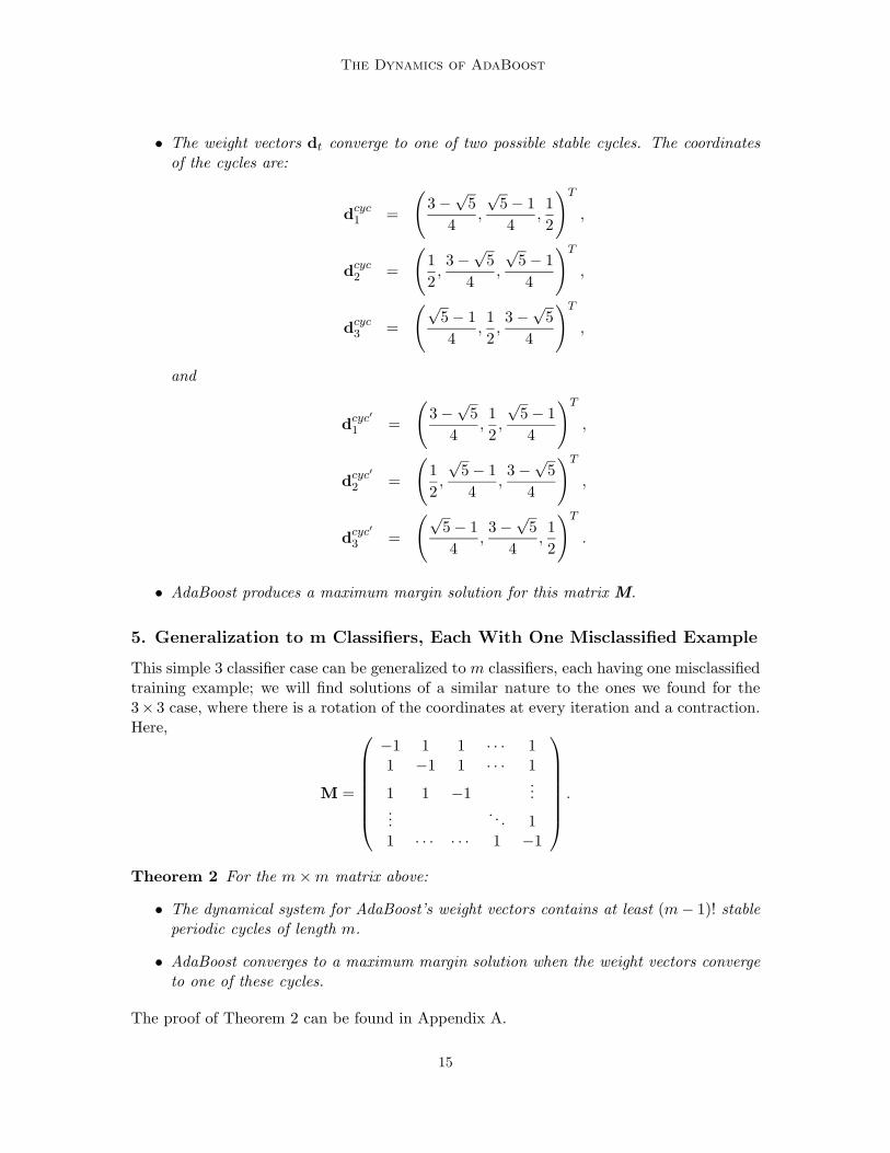
• The weight vectors dt converge to one of two possible stable cycles. The coordinatesof the cycles are:
dcyc1 =
(3 −
√5
4,
√5 − 1
4,1
2
)T
,
dcyc2 =
(1
2,3 −
√5
4,
√5 − 1
4
)T
,
dcyc3 =
(√5 − 1
4,1
2,3 −
√5
4
)T
,
and
dcyc′
1 =
(3 −
√5
4,1
2,
√5 − 1
4
)T
,
dcyc′
2 =
(1
2,
√5 − 1
4,3 −
√5
4
)T
,
dcyc′
3 =
(√5 − 1
4,3 −
√5
4,1
2
)T
.
• AdaBoost produces a maximum margin solution for this matrix M.
5. Generalization to m Classifiers, Each With One Misclassified Example
This simple 3 classifier case can be generalized to m classifiers, each having one misclassifiedtraining example; we will find solutions of a similar nature to the ones we found for the3× 3 case, where there is a rotation of the coordinates at every iteration and a contraction.Here,
M =
−1 1 1 · · · 11 −1 1 · · · 1
1 1 −1...
.... . . 1
1 · · · · · · 1 −1
.
Theorem 2 For the m × m matrix above:
• The dynamical system for AdaBoost’s weight vectors contains at least (m − 1)! stableperiodic cycles of length m.
• AdaBoost converges to a maximum margin solution when the weight vectors convergeto one of these cycles.
The proof of Theorem 2 can be found in Appendix A.
15
Rudin, Daubechies, Schapire
6. Identically Classified Examples and Manifolds of Cycles
In this section, we show how manifolds of cycles appear automatically from cyclic dynamicswhen there are sets of identically classified training examples. We show that the manifoldsof cycles that arise from a variation of the 3 × 3 case are stable. One should think of a“manifold of cycles” as a continuum of cycles; starting from a position on any cycle, ifwe move along the directions defined by the manifold, we will find starting positions forinfinitely many other cycles. These manifolds are interesting from a theoretical viewpoint.In addition, their existence and stability will be an essential part of the proof of Theorem 7.
A set of training examples I is identically classified if each pair of training examples iand i′ contained in I satisfy yihj(xi) = yi′hj(xi′) ∀j. That is, the rows i and i′ of matrix M
are identical; training examples i and i′ are misclassified by the same set of weak classifiers.When AdaBoost cycles, it treats each set of identically classified training examples as onetraining example, in a specific sense we will soon describe.
For convenience of notation, we will remove the ‘cyc’ notation so that d1 is a positionwithin the cycle (or equivalently, we could make the assumption that AdaBoost starts on acycle). Say there exists a cycle such that d1,i > 0 ∀i ∈ I, where d1 is a position within thecycle and M possesses some identically classified examples I. (I is not required to includeall examples identically classified with i ∈ I.) We know that for each pair of identicallyclassified examples i and i′ in I, we have Mijt
= Mi′jt∀t = 1, ..., T . Let perturbation
a ∈ Rm obey:
∑
i∈I
ai = 0, and also ai = 0 for i /∈ I.
Now, let da1 := d1 + a. We accept only perturbations a so that the perturbation does not
affect the value of any jt in the cycle. That is, we assume each component of a is sufficientlysmall; since the dynamical system defined by AdaBoost is piecewise continuous, it is possibleto choose a small enough so the perturbed trajectory is still close to the original trajectoryafter T iterations. Also, da
1 must still be a valid distribution, so it must obey the constraint
16
The Dynamics of AdaBoost
da1 ∈ ∆m, i.e.,
∑i ai = 0 as we have specified. Choose any elements i and i′ ∈ I. Now,
ra1 = (da
1TM)j1 = (d1
TM)j1 + (aTM)j1 = r1 +∑
i∈I
aiMij1= r1 + Mi′j1
∑
i∈I
ai = r1
da2,i =
da1,i
1 + Mij1ra1
=da
1,i
1 + Mij1r1=
d1,i
1 + Mij1r1+
1
1 + Mi′j1r1ai = d2,i +
1
1 + Mi′j1r1ai
ra2 = (da
2TM)j2 = (d2
TM)j2 +1
1 + Mi′j1r1(aTM)j2 = r2 +
1
1 + Mi′j1r1
∑
i∈I
aiMij2
= r2 +Mi′j2
1 + Mi′j1r1
∑
i∈I
ai = r2
da2,i =
da2,i
1 + Mij2ra2
=da
2,i
1 + Mij2r2=
d2,i
1 + Mij2r2+
1
(1 + Mi′j2r2)(1 + Mi′j1r1)ai
= d3,i +1
(1 + Mi′j2r2)(1 + Mi′j1r1)ai
...
daT+1,i = dT+1,i +
1∏T
t=1(1 + Mi′jtrt)
ai = d1,i + ai = da1,i.
The cycle condition was used in the last line. This calculation shows that if we perturbany cycle in the directions defined by I, we will find another cycle. An entire manifoldof cycles then exists, corresponding to the possible nonzero acceptable perturbations a.Effectively, the perturbation shifts the distribution among examples in I, with the totalweight remaining the same. For example, if a cycle exists containing vector d1 with d1,1 =.20, d1,2 = .10, and d1,3 = .30, where {1, 2, 3} ⊂ I, then a cycle with d1,1 = .22, d1,2 = .09,and d1,3 = .29 also exists, assuming none of the jt’s change; in this way, groups of identicallydistributed examples may be treated as one example, because they must share a single totalweight (again, only within the region where none of the jt’s change).
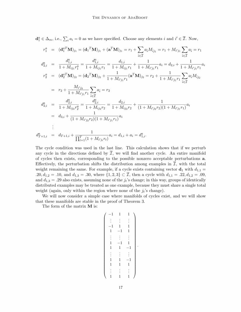
We will now consider a simple case where manifolds of cycles exist, and we will showthat these manifolds are stable in the proof of Theorem 3.
The form of the matrix M is:
−1 1 1...
......
−1 1 11 −1 1...
......
1 −1 11 1 −1...
......
1 1 −11 1 1...
......
1 1 1
.
17
Rudin, Daubechies, Schapire
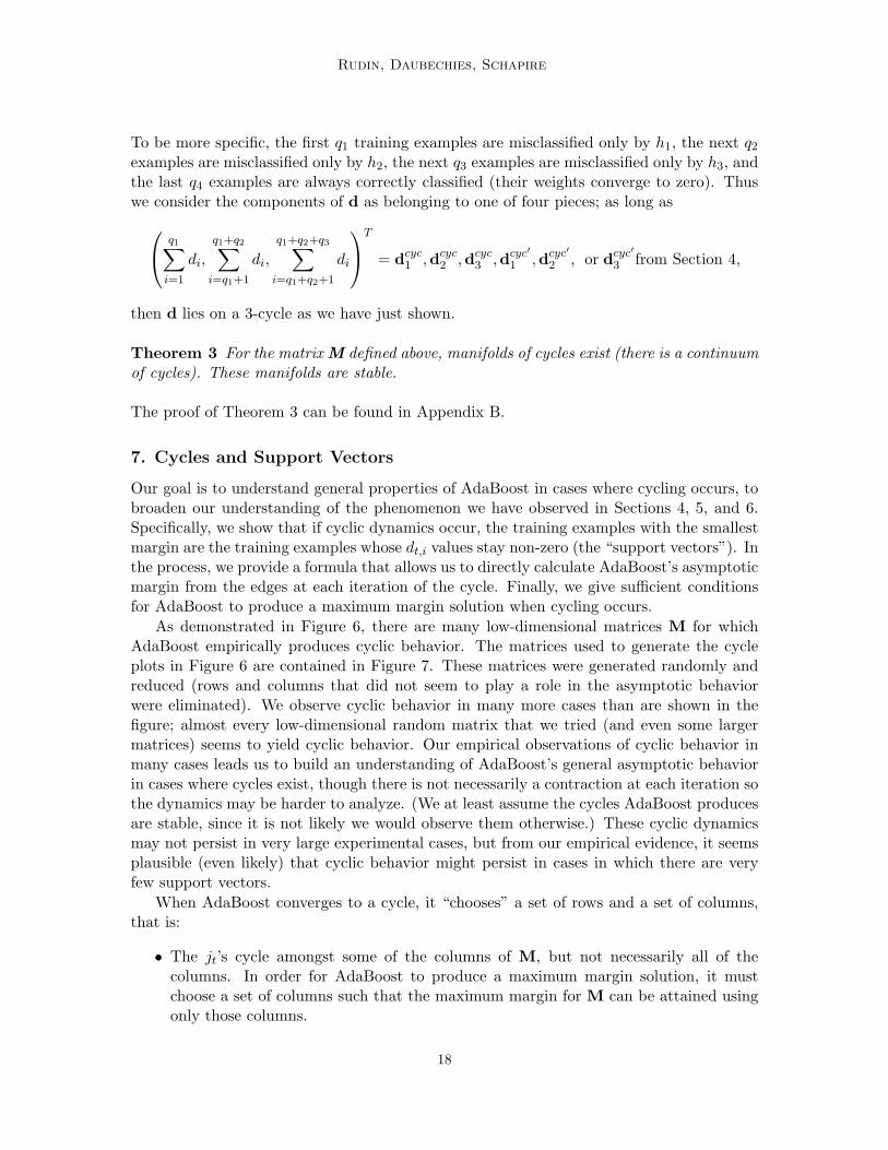
To be more specific, the first q1 training examples are misclassified only by h1, the next q2
examples are misclassified only by h2, the next q3 examples are misclassified only by h3, andthe last q4 examples are always correctly classified (their weights converge to zero). Thuswe consider the components of d as belonging to one of four pieces; as long as
q1∑
i=1
di,
q1+q2∑
i=q1+1
di,
q1+q2+q3∑
i=q1+q2+1
di
T
= dcyc1 ,dcyc
2 ,dcyc3 ,dcyc′
1 ,dcyc′
2 , or dcyc′
3 from Section 4,
then d lies on a 3-cycle as we have just shown.
Theorem 3 For the matrix M defined above, manifolds of cycles exist (there is a continuumof cycles). These manifolds are stable.
The proof of Theorem 3 can be found in Appendix B.
7. Cycles and Support Vectors
Our goal is to understand general properties of AdaBoost in cases where cycling occurs, tobroaden our understanding of the phenomenon we have observed in Sections 4, 5, and 6.Specifically, we show that if cyclic dynamics occur, the training examples with the smallestmargin are the training examples whose dt,i values stay non-zero (the “support vectors”). Inthe process, we provide a formula that allows us to directly calculate AdaBoost’s asymptoticmargin from the edges at each iteration of the cycle. Finally, we give sufficient conditionsfor AdaBoost to produce a maximum margin solution when cycling occurs.
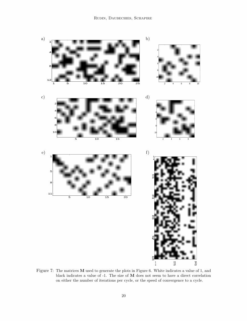
As demonstrated in Figure 6, there are many low-dimensional matrices M for whichAdaBoost empirically produces cyclic behavior. The matrices used to generate the cycleplots in Figure 6 are contained in Figure 7. These matrices were generated randomly andreduced (rows and columns that did not seem to play a role in the asymptotic behaviorwere eliminated). We observe cyclic behavior in many more cases than are shown in thefigure; almost every low-dimensional random matrix that we tried (and even some largermatrices) seems to yield cyclic behavior. Our empirical observations of cyclic behavior inmany cases leads us to build an understanding of AdaBoost’s general asymptotic behaviorin cases where cycles exist, though there is not necessarily a contraction at each iteration sothe dynamics may be harder to analyze. (We at least assume the cycles AdaBoost producesare stable, since it is not likely we would observe them otherwise.) These cyclic dynamicsmay not persist in very large experimental cases, but from our empirical evidence, it seemsplausible (even likely) that cyclic behavior might persist in cases in which there are veryfew support vectors.
When AdaBoost converges to a cycle, it “chooses” a set of rows and a set of columns,that is:
• The jt’s cycle amongst some of the columns of M, but not necessarily all of thecolumns. In order for AdaBoost to produce a maximum margin solution, it mustchoose a set of columns such that the maximum margin for M can be attained usingonly those columns.
18

The Dynamics of AdaBoost
a) b)
0 0.1 0.2 0.30
0.1
0.25
0.35
dt,1
d t,2
0 0.1 0.3 0.4 0.50
0.05
0.15
0.2
0.25
dt,1
d t,2
c) d)
0 0.05 0.15 0.250
0.05
0.25
0.35
dt,1
d t,2
0 0.1 0.2 0.30
0.1
0.3
0.4
dt,1
d t,2
e) f)
0 0.1 0.35 0.450
0.1
0.4
0.5
dt,1
d t,2
0 0.05 0.15 0.20
0.05
0.15
0.2
dt,11
d t,12
Figure 6: Examples of cycles from randomly generated matrices M. An image of M for each plotappears in Figure 7. These plots show a projection onto the first two components ofAdaBoost’s weight vector, e.g., the axes might be dt,1 vs. dt,2. Smaller circles indicateearlier iterations, and larger circles indicate later iterations. For (a), (d) and (f), 400iterations were plotted, and for (b) and (e), 300 iterations were plotted. Plot (c) shows5500 iterations, but only every 20th iteration was plotted. This case took longer toconverge, and converged to a simple 3-cycle.
19
Rudin, Daubechies, Schapire
a) b)
1 5 10 15 20 25
1
4
8
12
2 4 6 8 10
2
4
6
8
10
c) d)
5 10 15
2
4
6
8
10
2 4 6 8
2
4
6
8
10
e) f)
5 10 15 20
1
5
8
11
1 10 20
1
10
20
30
40
50
Figure 7: The matrices M used to generate the plots in Figure 6. White indicates a value of 1, andblack indicates a value of -1. The size of M does not seem to have a direct correlationon either the number of iterations per cycle, or the speed of convergence to a cycle.
20

The Dynamics of AdaBoost
• The values of dt,i (for a fixed value of i) are either always 0 or always strictly positivethroughout the cycle. A support vector is a training example i such that the dt,i’s inthe cycle are strictly positive. These support vectors are similar to the support vectorsof a support vector machine in that they all attain the minimum margin over trainingexamples (as we will show). These are training examples that AdaBoost concentratesthe hardest on. The remaining training examples have zero weight throughout thecycle; these are the examples that are easier for the algorithm to classify, since theyhave margin larger than the support vectors. For support vectors, the cycle conditionholds,
∏Tt=1(1 + Mijt
rcyct ) = 1. (This holds by Step 3 of the iterated map.) For non-
support vectors,∏T
t=1(1 + Mijtrcyct ) > 1 so the dt,i’s converge to 0 (the cycle must be
stable).
Theorem 4 AdaBoost produces the same margin for each support vector and larger marginsfor other training examples. This margin can be expressed in terms of the cycle parametersrcyc1 , ..., rcyc
T .
Proof Assume AdaBoost is cycling. Assume d1 is within the cycle for ease of notation.The cycle produces a normalized output λcyc := limt→∞ λt/||λt||1 for AdaBoost. (Thislimit always converges when AdaBoost converges to a cycle.) Denote
zcyc :=T∑
t=1
αt =T∑
t=1
1
2ln
(1 + rt
1 − rt
).
Let i be a support vector. Then,
(Mλcyc)i =1
zcyc
T∑
t=1
Mijtαt =
1
zcyc
T∑
t=1
Mijt
1
2ln
(1 + rt
1 − rt
)
=1
2zcyc
T∑
t=1
ln
(1 + Mijt
rt
1 − Mijtrt
)=
1
2zcyc
ln
[T∏
t=1
1 + Mijtrt
1 − Mijtrt
]
=1
2zcyc
ln
(T∏
t=1
1 + Mijtrt
1 − Mijtrt
)(T∏
t=1
1
(1 + Mijtrt)
)2
=1
2zcyc
ln
[T∏
t=1
1
(1 − Mijtrt)(1 + Mijt
rt)
]
=1
2zcyc
ln
[T∏
t=1
1
1 − r2t
]= −1
2
ln∏T
t=1 (1 − r2t )
∑Tt=1
12 ln
(1+r
t
1−rt
)
= − ln∏T
t=1(1 − r2t )
ln∏T
t=1
(1+r
t
1−rt
) . (5)
The first line uses the definition of αt from the AdaBoost algorithm, the second line usesthe fact that M is binary, the third line uses the fact that i is a support vector, i.e.,∏T
t=1(1 + Mijtrt) = 1. Since the value in (5) is independent of i, this is the value of the
21

Rudin, Daubechies, Schapire
margin that AdaBoost assigns to every support vector i. We denote the value in (5) asµcycle, which is only a function of the cycle parameters, i.e., the edge values.
Now we show that every non-support vector achieves a larger margin than µcycle. For
a non-support vector i, we have∏T
t=1(1 + Mijtrt) > 1, that is, the cycle is stable. Thus,
0 > ln
[1∏T
t=1(1+Mijt
rt)
]2
. Now,
(Mλcyc)i =1
zcyc
T∑
t=1
Mijtαt =
1
2zcyc
ln
[∏t(1 + Mijt
rt)∏t(1 − Mijt
rt)
]
>1
2zcyc
ln
[∏t(1 + Mijt
rt)∏t(1 − Mijt
rt)
]+
1
2zcyc
ln
[1∏
t(1 + Mijtrt)
]2
=− ln
∏Tt=1(1 − r2
t )
ln∏T
t=1
(1+r
t
1−rt
) = µcycle.
Thus, non-support vectors achieve larger margins than support vectors.
The previous theorem shows that the asymptotic margin of the support vectors is thesame as the asymptotic margin produced by AdaBoost; this asymptotic margin can be di-rectly computed using (5). AdaBoost may not always produce a maximum margin solution,as we will see in Sections 8 and 9; however, there are sufficient conditions such that Ada-Boost will automatically produce a maximum margin solution when cycling occurs. Beforewe state these conditions, we define the matrix Mcyc ∈ {−1, 1}mcyc×ncyc , which containscertain rows and columns of M. To construct Mcyc from M, we choose only the rows of M
that correspond to support vectors (eliminating the others, whose weights vanish anyway),and choose only the columns of M corresponding to weak classifiers that are chosen in thecycle (eliminating the others, which are never chosen after cycling begins anyway). Here,mcyc is the number of support vectors chosen by AdaBoost, and ncyc is the number of weakclassifiers in the cycle.
Theorem 5 Suppose AdaBoost is cycling, and that the following are true:
1.
maxλ∈∆ncyc
mini
(Mcycλ)i = maxλ∈∆n
mini
(Mλ)i = ρ
(AdaBoost cycles among columns of M that can be used to produce a maximum marginsolution.)
2. There exists λρ ∈ ∆ncycsuch that (Mcycλρ)i = ρ for i = 1, ..., mcyc. (AdaBoost
chooses support vectors corresponding to a maximum margin solution for Mcyc.)
3. The matrix Mcyc is invertible.
Then AdaBoost produces a maximum margin solution.
22

The Dynamics of AdaBoost
The first two conditions specify that AdaBoost cycles among columns of M that can beused to produce a maximum margin solution, and chooses support vectors correspondingto this solution. The first condition specifies that the maximum margin, ρ, (correspondingto the matrix M) must be the same as the maximum margin corresponding to Mcyc. Sincethe cycle is stable, all other training examples achieve larger margins; hence ρ is the bestpossible margin Mcyc can achieve. The second condition specifies that there is at least oneanalytical solution λρ such that all training examples of Mcyc achieve a margin of exactlyρ.
Proof By Theorem 4, AdaBoost will produce the same margin for all of the rows of Mcyc,since they are all support vectors. We denote the value of this margin by µcycle.
Let χmcyc:= (1, 1, 1, . . . , 1)T , with mcyc components. From 2, we are guaranteed the
existence of λρ such that
Mcycλρ = ρχmcyc.
We already know
Mcycλcyc = µcycleχmcyc
since all rows are support vectors for our cycle. Since Mcyc is invertible,
λcyc = µcycleM−1cycχmcyc
and λρ = ρM−1cycχmcyc
,
so we have λcyc = constant · λρ. Since λcyc and λρ must both be normalized, the constantmust be 1. Thus ρ = µcycle.
It is possible for the conditions of Theorem 5 not to hold, for example, condition 1 doesnot hold in the examples of Sections 8 and 9; in these cases, a maximum margin solutionis not achieved. It can be shown that the first two conditions are necessary but the thirdone is not. It is not hard to understand the necessity of the first two conditions; if it isnot possible to produce a maximum margin solution using the weak classifiers and supportvectors AdaBoost has chosen, then it is not possible for AdaBoost to produce a maximummargin solution. The third condition is thus quite important, since it allows us to uniquelyidentify λcyc. Condition 3 does hold for the cases studied in Sections 4 and 5.
8. Non-Optimal AdaBoost Does Not Necessarily Converge to a
Maximum Margin Solution, Even if Optimal AdaBoost Does
Based on large scale experiments and a gap in theoretical bounds, Ratsch and Warmuth [16]conjectured that AdaBoost does not necessarily converge to a maximum margin classifierin the non-optimal case, i.e., that AdaBoost is not robust in this sense. In practice, theweak classifiers are generated by CART or another weak learning algorithm, implying thatthe choice need not always be optimal.
We will consider a 4× 5 matrix M for which AdaBoost fails to converge to a maximummargin solution if the edge at each iteration is required only to exceed ρ (the non-optimalcase). That is, we show that “non-optimal AdaBoost” (AdaBoost in the non-optimal case)may not converge to a maximum margin solution, even in cases where “optimal AdaBoost”does.
23
Rudin, Daubechies, Schapire
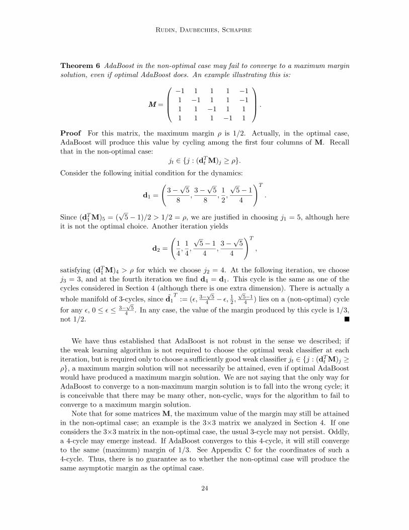
Theorem 6 AdaBoost in the non-optimal case may fail to converge to a maximum marginsolution, even if optimal AdaBoost does. An example illustrating this is:
M =
−1 1 1 1 −11 −1 1 1 −11 1 −1 1 11 1 1 −1 1
.
Proof For this matrix, the maximum margin ρ is 1/2. Actually, in the optimal case,AdaBoost will produce this value by cycling among the first four columns of M. Recallthat in the non-optimal case:
jt ∈ {j : (dTt M)j ≥ ρ}.
Consider the following initial condition for the dynamics:
d1 =
(3 −
√5
8,3 −
√5
8,1
2,
√5 − 1
4
)T
.
Since (dT1 M)5 = (
√5 − 1)/2 > 1/2 = ρ, we are justified in choosing j1 = 5, although here
it is not the optimal choice. Another iteration yields
d2 =
(1
4,1
4,
√5 − 1
4,3 −
√5
4
)T
,
satisfying (dT1 M)4 > ρ for which we choose j2 = 4. At the following iteration, we choose
j3 = 3, and at the fourth iteration we find d4 = d1. This cycle is the same as one of thecycles considered in Section 4 (although there is one extra dimension). There is actually a
whole manifold of 3-cycles, since d1T
:= (ε, 3−√
54 − ε, 1
2 ,√
5−14 ) lies on a (non-optimal) cycle
for any ε, 0 ≤ ε ≤ 3−√
54 . In any case, the value of the margin produced by this cycle is 1/3,
not 1/2.
We have thus established that AdaBoost is not robust in the sense we described; ifthe weak learning algorithm is not required to choose the optimal weak classifier at eachiteration, but is required only to choose a sufficiently good weak classifier jt ∈ {j : (dT
t M)j ≥ρ}, a maximum margin solution will not necessarily be attained, even if optimal AdaBoostwould have produced a maximum margin solution. We are not saying that the only way forAdaBoost to converge to a non-maximum margin solution is to fall into the wrong cycle; itis conceivable that there may be many other, non-cyclic, ways for the algorithm to fail toconverge to a maximum margin solution.
Note that for some matrices M, the maximum value of the margin may still be attainedin the non-optimal case; an example is the 3×3 matrix we analyzed in Section 4. If oneconsiders the 3×3 matrix in the non-optimal case, the usual 3-cycle may not persist. Oddly,a 4-cycle may emerge instead. If AdaBoost converges to this 4-cycle, it will still convergeto the same (maximum) margin of 1/3. See Appendix C for the coordinates of such a4-cycle. Thus, there is no guarantee as to whether the non-optimal case will produce thesame asymptotic margin as the optimal case.
24
The Dynamics of AdaBoost
0 50 150 200−0.5
0
0.20.30.40.5
Iterations
Mar
gin
Optimal AdaBoost
Non−Optimal AdaBoost
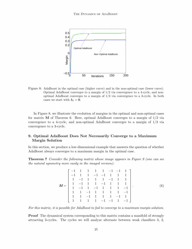
Figure 8: AdaBoost in the optimal case (higher curve) and in the non-optimal case (lower curve).Optimal AdaBoost converges to a margin of 1/2 via convergence to a 4-cycle, and non-optimal AdaBoost converges to a margin of 1/3 via convergence to a 3-cycle. In bothcases we start with λ1 = 0.
In Figure 8, we illustrate the evolution of margins in the optimal and non-optimal casesfor matrix M of Theorem 6. Here, optimal AdaBoost converges to a margin of 1/2 viaconvergence to a 4-cycle, and non-optimal AdaBoost converges to a margin of 1/3 viaconvergence to a 3-cycle.
9. Optimal AdaBoost Does Not Necessarily Converge to a Maximum
Margin Solution
In this section, we produce a low-dimensional example that answers the question of whetherAdaBoost always converges to a maximum margin in the optimal case.
Theorem 7 Consider the following matrix whose image appears in Figure 9 (one can seethe natural symmetry more easily in the imaged version):
M =
−1 1 1 1 1 −1 −1 1−1 1 1 −1 −1 1 1 11 −1 1 1 1 −1 1 11 −1 1 1 −1 1 1 11 −1 1 −1 1 1 1 −11 1 −1 1 1 1 1 −11 1 −1 1 1 1 −1 11 1 1 1 −1 −1 1 −1
. (6)
For this matrix, it is possible for AdaBoost to fail to converge to a maximum margin solution.
Proof The dynamical system corresponding to this matrix contains a manifold of stronglyattracting 3-cycles. The cycles we will analyze alternate between weak classifiers 3, 2,
25
Rudin, Daubechies, Schapire
2 4 6 8
1
2
3
4
5
6
7
8
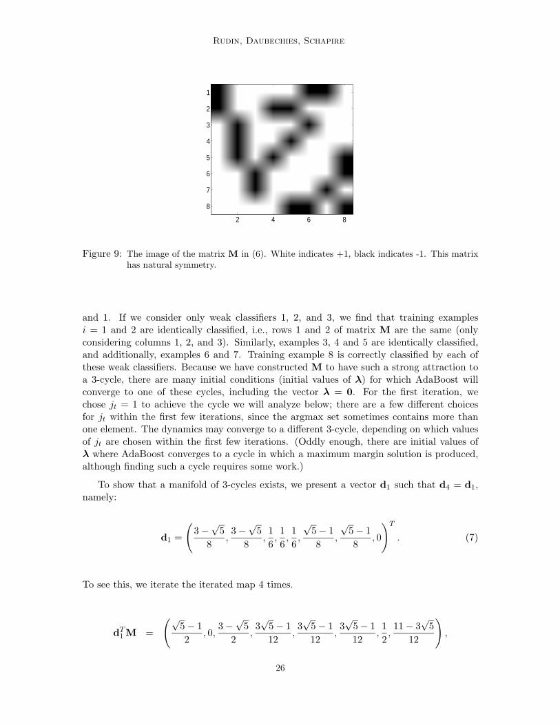
Figure 9: The image of the matrix M in (6). White indicates +1, black indicates -1. This matrixhas natural symmetry.
and 1. If we consider only weak classifiers 1, 2, and 3, we find that training examplesi = 1 and 2 are identically classified, i.e., rows 1 and 2 of matrix M are the same (onlyconsidering columns 1, 2, and 3). Similarly, examples 3, 4 and 5 are identically classified,and additionally, examples 6 and 7. Training example 8 is correctly classified by each ofthese weak classifiers. Because we have constructed M to have such a strong attraction toa 3-cycle, there are many initial conditions (initial values of λ) for which AdaBoost willconverge to one of these cycles, including the vector λ = 0. For the first iteration, wechose jt = 1 to achieve the cycle we will analyze below; there are a few different choicesfor jt within the first few iterations, since the argmax set sometimes contains more thanone element. The dynamics may converge to a different 3-cycle, depending on which valuesof jt are chosen within the first few iterations. (Oddly enough, there are initial values ofλ where AdaBoost converges to a cycle in which a maximum margin solution is produced,although finding such a cycle requires some work.)
To show that a manifold of 3-cycles exists, we present a vector d1 such that d4 = d1,namely:
d1 =
(3 −
√5
8,3 −
√5
8,1
6,1
6,1
6,
√5 − 1
8,
√5 − 1
8, 0
)T
. (7)
To see this, we iterate the iterated map 4 times.
dT1 M =
(√5 − 1
2, 0,
3 −√
5
2,3√
5 − 1
12,3√
5 − 1
12,3√
5 − 1
12,1
2,11 − 3
√5
12
),
26
The Dynamics of AdaBoost
and here j1 = 1,
d2 =
(1
4,1
4,
√5 − 1
12,
√5 − 1
12,
√5 − 1
12,3 −
√5
8,3 −
√5
8, 0
)T
dT2 M =
(0,
3 −√
5
2,
√5 − 1
2,4 −
√5
6,4 −
√5
6,4 −
√5
6,
√5 − 1
4,5 +
√5
12
),
and here j2 = 3,
d3 =
(√5 − 1
8,
√5 − 1
8,3 −
√5
12,3 −
√5
12,3 −
√5
12,1
4,1
4, 0
)T
dT3 M =
(3 −
√5
2,
√5 − 1
2, 0,
3
4−
√5
12,3
4−
√5
12,3
4−
√5
12,3 −
√5
4,
√5
6
),
and here, j3 = 2, and then d4 = d1.
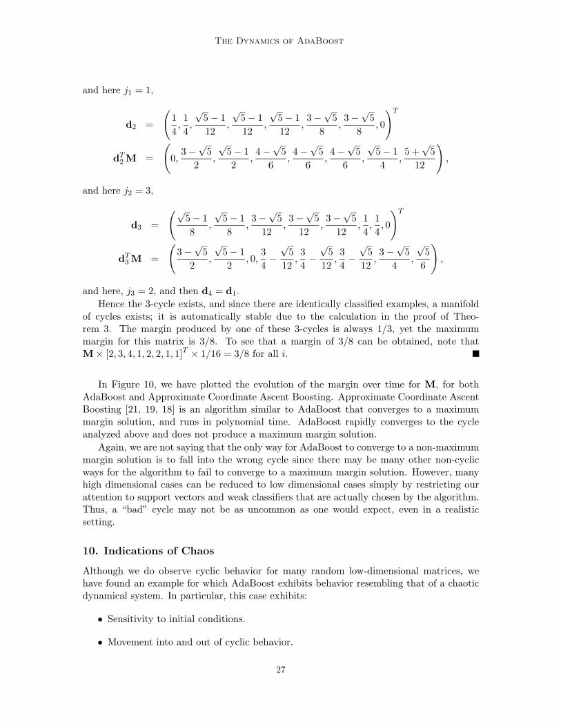
Hence the 3-cycle exists, and since there are identically classified examples, a manifoldof cycles exists; it is automatically stable due to the calculation in the proof of Theo-rem 3. The margin produced by one of these 3-cycles is always 1/3, yet the maximummargin for this matrix is 3/8. To see that a margin of 3/8 can be obtained, note thatM × [2, 3, 4, 1, 2, 2, 1, 1]T × 1/16 = 3/8 for all i.
In Figure 10, we have plotted the evolution of the margin over time for M, for bothAdaBoost and Approximate Coordinate Ascent Boosting. Approximate Coordinate AscentBoosting [21, 19, 18] is an algorithm similar to AdaBoost that converges to a maximummargin solution, and runs in polynomial time. AdaBoost rapidly converges to the cycleanalyzed above and does not produce a maximum margin solution.
Again, we are not saying that the only way for AdaBoost to converge to a non-maximummargin solution is to fall into the wrong cycle since there may be many other non-cyclicways for the algorithm to fail to converge to a maximum margin solution. However, manyhigh dimensional cases can be reduced to low dimensional cases simply by restricting ourattention to support vectors and weak classifiers that are actually chosen by the algorithm.Thus, a “bad” cycle may not be as uncommon as one would expect, even in a realisticsetting.
10. Indications of Chaos
Although we do observe cyclic behavior for many random low-dimensional matrices, wehave found an example for which AdaBoost exhibits behavior resembling that of a chaoticdynamical system. In particular, this case exhibits:
• Sensitivity to initial conditions.
• Movement into and out of cyclic behavior.
27
Rudin, Daubechies, Schapire
0 50 100−0.1
0.2
0.3
0.4
Iterations
Mar
gin
Figure 10: AdaBoost (lower curve) and Approximate Coordinate Ascent Boosting (higher curve),using the 8 × 8 matrix M given in Section 9 and initial condition λ = 0. AdaBoostconverges to a margin of 1/3, yet the value of ρ is 3/8. Thus, AdaBoost does notconverge to a maximum margin solution for this matrix M.
The matrix M we consider for this section is given in Figure 7(a).
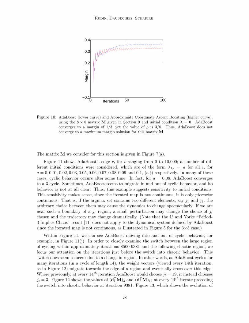
Figure 11 shows AdaBoost’s edge rt for t ranging from 0 to 10,000; a number of dif-ferent initial conditions were considered, which are of the form λ1,i = a for all i, fora = 0, 0.01, 0.02, 0.03, 0.05, 0.06, 0.07, 0.08, 0.09 and 0.1, (a-j) respectively. In many of thesecases, cyclic behavior occurs after some time. In fact, for a = 0.08, AdaBoost convergesto a 3-cycle. Sometimes, AdaBoost seems to migrate in and out of cyclic behavior, and itsbehavior is not at all clear. Thus, this example suggests sensitivity to initial conditions.This sensitivity makes sense, since the iterated map is not continuous, it is only piecewisecontinuous. That is, if the argmax set contains two different elements, say j1 and j2, thearbitrary choice between them may cause the dynamics to change spectacularly. If we arenear such a boundary of a jt region, a small perturbation may change the choice of jt
chosen and the trajectory may change dramatically. (Note that the Li and Yorke “Period-3-Implies-Chaos” result [11] does not apply to the dynamical system defined by AdaBoostsince the iterated map is not continuous, as illustrated in Figure 5 for the 3×3 case.)
Within Figure 11, we can see AdaBoost moving into and out of cyclic behavior, forexample, in Figure 11(j). In order to closely examine the switch between the large regionof cycling within approximately iterations 8500-9381 and the following chaotic region, wefocus our attention on the iterations just before the switch into chaotic behavior. Thisswitch does seem to occur due to a change in region. In other words, as AdaBoost cycles formany iterations (in a cycle of length 14), the weight vectors (viewed every 14th iteration,as in Figure 12) migrate towards the edge of a region and eventually cross over this edge.Where previously, at every 14th iteration AdaBoost would choose jt = 19, it instead choosesjt = 3. Figure 12 shows the values of (dT
t M)3 and (dTt M)19 at every 14th iterate preceding
the switch into chaotic behavior at iteration 9381. Figure 13, which shows the evolution of
28

The Dynamics of AdaBoost
two components of the weight vector, also illustrates the switches into and out of chaoticbehavior.
Eventually, the dynamics drift back towards the same cycle and actually seem to con-verge to it, as shown in Figure 14(a). Here, the weight vectors do not cross regions, sincethe values of the largest two components of (dTM) do not cross, as shown in Figure 14(b).
Thus, there are many open questions regarding AdaBoost’s dynamics that could helpus understand its asymptotic behavior; for example, is AdaBoost chaotic in some cases ordoes it perhaps always produce cyclic behavior asymptotically?
11. Conclusions
We have used the nonlinear iterated map defined by AdaBoost to understand its update rulein low-dimensional cases and uncover remarkable cyclic dynamics. We describe many as-pects of AdaBoost’s dynamical traits including the fact that AdaBoost does not necessarilyconverge to a maximum margin solution. We have also proved the conjecture that Ada-Boost is not robust to the choice of weak classifier. The key to answering these questionswas our analysis of cases in which AdaBoost’s asymptotic behavior could be completelydetermined. Thus an understanding of simple cases has yielded answers to important openquestions concerning AdaBoost’s large-scale asymptotic behavior.
We leave open many interesting questions. To what extent is AdaBoost chaotic? Forwhat cases does AdaBoost produce maximum margin solutions? Does AdaBoost alwaysexhibit cyclic behavior in the limit? If AdaBoost can behave chaotically without convergingto a cycle, how large does the matrix M need to be in order to produce such behavior?And finally, how does AdaBoost achieve its strong generalization performance if it does notsimply maximize the margin? We hope the analytical tools provided in this work, namelythe reduction of AdaBoost to a dynamical system and the analysis of its asymptotic behaviorin special cases, will help yield answers to these interesting questions.
References
[1] Leo Breiman. Arcing the edge. Technical Report 486, Statistics Department, University ofCalifornia at Berkeley, 1997.
[2] Leo Breiman. Arcing classifiers. The Annals of Statistics, 26(3):801–849, 1998.[3] Leo Breiman. Prediction games and arcing algorithms. Neural Computation, 11(7):1493–1517,
1999.[4] Michael Collins, Robert E. Schapire, and Yoram Singer. Logistic regression, AdaBoost and
Bregman distances. Machine Learning, 48(1/2/3), 2002.[5] Ayhan Demiriz, Kristin P. Bennett, and John Shawe-Taylor. Linear programming boosting via
column generation. Machine Learning, 46(1/2/3):225–254, 2002.[6] N. Duffy and D. Helmbold. A geometric approach to leveraging weak learners. In Computational
Learning Theory: Fourth European Conference, EuroCOLT ’99. Springer-Verlag, 1999.[7] Yoav Freund and Robert E. Schapire. A decision-theoretic generalization of on-line learning and
an application to boosting. Journal of Computer and System Sciences, 55(1):119–139, August1997.
[8] Jerome Friedman, Trevor Hastie, and Robert Tibshirani. Additive logistic regression: A statis-tical view of boosting. The Annals of Statistics, 38(2):337–374, April 2000.
[9] Adam J. Grove and Dale Schuurmans. Boosting in the limit: Maximizing the margin of learnedensembles. In Proceedings of the Fifteenth National Conference on Artificial Intelligence, 1998.
29
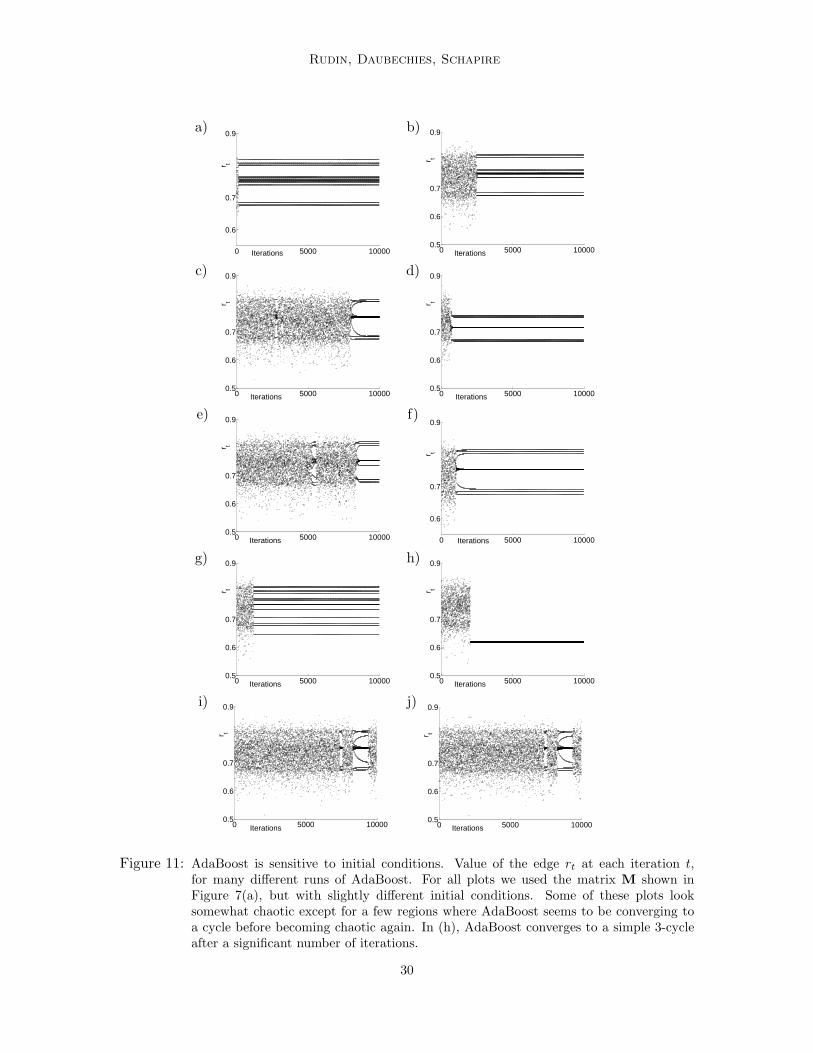
Rudin, Daubechies, Schapire
a) b)
0 5000 10000
0.6
0.7
0.9
Iterations
r t
0 5000 100000.5
0.6
0.7
0.9
Iterations
r t
c) d)
0 5000 100000.5
0.6
0.7
0.9
Iterations
r t
0 5000 100000.5
0.6
0.7
0.9
Iterations
r t
e) f)
0 5000 100000.5
0.6
0.7
0.9
Iterations
r t
0 5000 10000
0.6
0.7
0.9
Iterations
r t
g) h)
0 5000 100000.5
0.6
0.7
0.9
Iterations
r t
0 5000 100000.5
0.6
0.7
0.9
Iterations
r t
i) j)
0 5000 100000.5
0.6
0.7
0.9
Iterations
r t
0 5000 100000.5
0.6
0.7
0.9
Iterations
r t
Figure 11: AdaBoost is sensitive to initial conditions. Value of the edge rt at each iteration t,for many different runs of AdaBoost. For all plots we used the matrix M shown inFigure 7(a), but with slightly different initial conditions. Some of these plots looksomewhat chaotic except for a few regions where AdaBoost seems to be converging toa cycle before becoming chaotic again. In (h), AdaBoost converges to a simple 3-cycleafter a significant number of iterations.
30
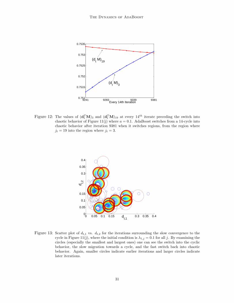
The Dynamics of AdaBoost
9241 9283 9339 93810.751
0.7515
0.752
0.7525
0.753
0.7535
Every 14th Iteration
(dt M)
19
(dt M)
3
Figure 12: The values of (dTt M)3 and (dT
t M)19 at every 14th iterate preceding the switch intochaotic behavior of Figure 11(j) where a = 0.1. AdaBoost switches from a 14-cycle intochaotic behavior after iteration 9381 when it switches regions, from the region wherejt = 19 into the region where jt = 3.
0 0.05 0.1 0.15 0.3 0.35 0.40
0.05
0.1
0.15
0.3
0.35
0.4
dt,1
d t,2
Figure 13: Scatter plot of dt,1 vs. dt,2 for the iterations surrounding the slow convergence to thecycle in Figure 11(j), where the initial condition is λ1,j = 0.1 for all j. By examining thecircles (especially the smallest and largest ones) one can see the switch into the cyclicbehavior, the slow migration towards a cycle, and the fast switch back into chaoticbehavior. Again, smaller circles indicate earlier iterations and larger circles indicatelater iterations.
31
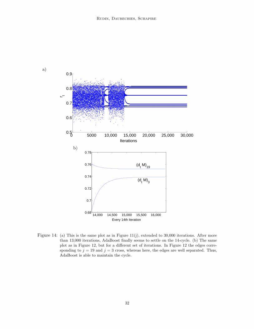
Rudin, Daubechies, Schapire
a)
0 5000 10,000 15,000 20,000 25,000 30,0000.5
0.6
0.7
0.8
0.9
Iterations
r t
b)
14,000 14,500 15,000 15,500 16,0000.68
0.7
0.72
0.74
0.76
0.78
Every 14th Iteration
(dt M)
19
(dt M)
3
Figure 14: (a) This is the same plot as in Figure 11(j), extended to 30,000 iterations. After morethan 13,000 iterations, AdaBoost finally seems to settle on the 14-cycle. (b) The sameplot as in Figure 12, but for a different set of iterations. In Figure 12 the edges corre-sponding to j = 19 and j = 3 cross, whereas here, the edges are well separated. Thus,AdaBoost is able to maintain the cycle.
32
The Dynamics of AdaBoost
[10] Vladimir Koltchinskii and Dmitry Panchenko. Empirical margin distributions and boundingthe generalization error of combined classifiers. The Annals of Statistics, 30(1), February 2002.
[11] T. Y. Li and J. A. Yorke. Period 3 implies chaos. Amer. Math. Monthly, 82(10):985–992, 1975.[12] Llew Mason, Jonathan Baxter, Peter Bartlett, and Marcus Frean. Boosting algorithms as
gradient descent. In Advances in Neural Information Processing Systems 12, 2000.[13] R. Meir and G. Ratsch. An introduction to boosting and leveraging. In S. Mendelson and
A. Smola, editors, Advanced Lectures on Machine Learning, LNCS, pages 119–184. SpringerVerlag, 2003.
[14] J. R. Quinlan. Bagging, boosting, and C4.5. In Proceedings of the Thirteenth National Confer-ence on Artificial Intelligence, pages 725–730, 1996.
[15] G. Ratsch, T. Onoda, and K.-R. Muller. Soft margins for AdaBoost. Machine Learning,42(3):287–320, 2001.
[16] Gunnar Ratsch and Manfred Warmuth. Efficient margin maximizing with boosting. unpublishedmanuscript, 2002.
[17] Saharon Rosset, Ji Zhu, and Trevor Hastie. Boosting as a regularized path to a maximummargin classifier. Journal of Machine Learning Research, 5:941–973, August 2004.
[18] Cynthia Rudin. Boosting, Margins and Dynamics. PhD thesis, Princeton University, April2004.
[19] Cynthia Rudin, Ingrid Daubechies, and Robert E. Schapire. On the dynamics of boosting. InAdvances in Neural Information Processing Systems 16, 2004.
[20] Cynthia Rudin, Robert E. Schapire, and Ingrid Daubechies. Analysis of boosting algorithmsusing the smooth margin function : A study of three algorithms. in preparation.
[21] Cynthia Rudin, Robert E. Schapire, and Ingrid Daubechies. Boosting based on a smoothmargin. In Proceedings of the Sixteenth Annual Conference on Computational Learning Theory,pages 502–517, 2004.
[22] Robert E. Schapire. The boosting approach to machine learning: An overview. In MSRIWorkshop on Nonlinear Estimation and Classification, 2002.
[23] Robert E. Schapire, Yoav Freund, Peter Bartlett, and Wee Sun Lee. Boosting the margin: Anew explanation for the effectiveness of voting methods. The Annals of Statistics, 26(5):1651–1686, October 1998.
[24] Abraham Wyner. Boosting and the exponential loss. In Proceedings of the Ninth AnnualConference on AI and Statistics, 2002.
Appendix A. Proof of Theorem 2
Let us first assume a cycle with rotating coordinates exists for this case, and then we will prove itsexistence and stability. Denote the first position in our cycle as follows (we drop the (cyc) notationhere):
d1 = (β1, · · · , βi, · · · , βm−1, βm)T ,
where 0 < β1 < β2 < · · · < βm. Note that βm = 12 , again because (dT
2 M)1 = 0 and∑
i d2,i = 1.Now,
dT1 M = ((1 − 2β1), · · · , (1 − 2βm−1), 0)T ,
so j1 = 1 and r1 = 1 − 2β1. Then, using the iterated map,
d2 =
(1
2,
β2
2(1 − β1), · · · ,
βi
2(1 − β1), · · · ,
βm−1
2(1 − β1),
βm
2(1 − β1)
)T
.
Assuming that the coordinates cycle,
βi−1 =βi
2(1 − β1)for i = 2, ...,m, (8)
33
Rudin, Daubechies, Schapire
in order for the current iterate to agree with the next iterate. This recursive relation gives
βi−(i−1) =βi
[2(1 − β1)]i−1,
so that
β1 =βm
[2(1 − β1)]m−1(9)
andβi = β1[2(1 − β1)]
i−1, for i = 1, ...,m. (10)
Thus, substituting (9) into (10), recalling that βm = 1/2,
βi =βm
[2(1 − β1)]m−1[2(1 − β1)]
i−1 =1
2[2(1 − β1)]
i−m. (11)
It remains to show that there is a viable solution for β1 to prove the existence of a cycle. (We requirea solution to obey β1 ≤ 1/m so that it is possible for
∑i d1,i = 1.) The condition
∑i d1,i = 1 can
be rewritten as:
1 =1
2
m∑
i=1
[2(1 − β1)]i−m.
Substituting ς = 2(1 − β1) and multiplying both sides by 2ςm−1, we have a geometric series:
2ςm−1 =
m∑
i=1
ςi−m+m−1 =
m∑
i=1
ςi−1 =1 − ςm
1 − ς,
that is,ςm − 2ςm−1 + 1 = 0. (12)
Substituting back for ς,2m(1 − β1)
m−1[(1 − β1) − 1] + 1 = 0,
or more simply,1 − β12
m(1 − β1)m−1 = 0.
To show a solution exists for m ≥ 4 (we have already handled the m = 3 case), we will applythe Intermediate Value Theorem to the function:
ϕ(β1,m) := 1 − β12m(1 − β1)
m−1.
We know ϕ(0,m) = 1 > 0. Consider
ϕ
(1
10,m
)= 1 − 2m 1
10
(9
10
)m−1
= 1 −(
9
5
)m1
9.
Plugging in m = 4, we find that ϕ(1/10, 4) = −104/625 < 0. On the other hand, extending thedefinition of ϕ to non-integer values of m, we have:
∂ϕ(1/10,m)
∂m= −1
9
[ln
(9
5
)](9
5
)m
< 0 for all m ≥ 4.
Hence, ϕ(1/10,m) ≤ −104/625 < 0 for all m ≥ 4. By the Intermediate Value Theorem, there is aroot β1 of ϕ(·,m) for any m ≥ 4 with 0 ≤ β1 ≤ 1/10. Since
∂ϕ(β1,m)
∂β1= 2m(1 − β1)
m−2(mβ1 − 1),
34

The Dynamics of AdaBoost
we have ∂ϕ
∂β1
(β1,m) = 0 only when β1 = 1/m, and that ϕ(·,m) decreases for 0 ≤ β1 < 1/m and
increases for β1 > 1/m (where β1 < 1). If m ≤ 10, since ϕ(·,m) decreases for 0 ≤ β1 < 1/m, theIntermediate Value Theorem provides the unique root 0 ≤ β1 ≤ 1/10 ≤ 1/m. If m > 10, ϕ(·,m)decreases for 0 ≤ β1 < 1/m and increases to the value ϕ(1/10,m), which is negative. Thus, there isa unique root 0 ≤ β1 ≤ 1/m. Hence, the root exists and is unique for m ≥ 4. Now we have shownthe existence and uniqueness of our cycle, namely the cycle starting from
d1 =(β1, 2β1(1 − β1), 4β2
1(1 − β1)2, ..., 1/2
)T.
Of course, this is not the only periodic orbit. Any permutation of the components in d1 willlie on a periodic cycle. If (without loss of generality) we fix the first iteration of each cycle to startwith the same first component d1,i = β1, then the number of permutations of the other components(and thus the number of periodic cycles we have defined by relabelling the coordinates) is (m− 1)!.
We now show that these (m− 1)! cycles are stable. It is sufficient to show that just one cycle isstable, since the others are obtained by simply relabelling the order of the coordinates (without lossof generality say jt = t for t = 1, ...,m). We add a perturbation εa to d1, small enough so that noneof the jt’s chosen within the cycle are affected. (Note that choosing such a perturbation is possible,since the map is piecewise continuous, and β1 < ... < βm without equality between the βi’s. Thiswill ensure that no dt lies on the boundary of a region, so that the argmaxj(d
Tt M)j set contains
exactly one element.) Also, we require∑m
i=1 ai = 0 so the perturbed starting point still lies on thesimplex ∆m. Assume ‖a‖1 is O(1), and that ε is small. Our perturbed starting point is:
da1 := d1 + εa.
Now, since r1 = 1 − 2β1,
ra1 = (da
1TM)1 = (d1
T M)1 + ε(aT M)1 = 1 − 2β1 + ε(aT M)1.
Again we use the iterated map. Recall that βm = 12 , and da
2,1 = 12 . For all other i:
da2,i =
βi + εai
1 + ra1
=βi + εai
2 − 2β1 + ε(aT M)1.
To see whether the perturbation has shrunk due to the dynamics, we compute εa := da2 − d2. If
‖a‖1 ≤ C‖a‖1 where C is a constant less than 1, the map is a contraction. Recall that
d2 =
(1
2, β1, · · · , βm−1
)T
.
Thus,
εa1 = da2,1 − d2,1 = 0,
and for other i,
εai = da2,i − d2,i =
βi + εai
2 − 2β1 + ε(aT M)1− βi−1.
We are done with the i = 1 term. For all other terms, we will do an approximation to first order inε. Using a first order Taylor expansion 1
1+x≈ 1 − x, we obtain:
1
1 + ra1
=1
2 − 2β1 + ε(aT M)1=
1
2(1 − β1)(1 + ε(aT M)1
2(1−β1)
) ≈1 − ε(aT
M)12(1−β1)
2(1 − β1).
35

Rudin, Daubechies, Schapire
Our expansion yields:
εai = da2,i − d2,i ≈
(βi + εai)(1 − ε(aT
M)12(1−β1)
)
2(1 − β1)− βi−1.
Grouping terms in orders of ε, we can use (8) to show the first term vanishes, and we find:
εai ≈ 0 + ε
(ai
2(1 − β1)− βi(a
T M)14(1 − β1)2
)+ O(ε2), so that
ai ≈ ai
2(1 − β1)− βi(a
T M)14(1 − β1)2
+ O(ε).
We will show that the perturbation shrinks at every iteration. Since ε is small, we do not care aboutthe O(ε) contribution to ai. Recall that
∑i βi = 1, so that:
‖a‖1 ≤ 1
2(1 − β1)
m∑
i=1
|ai| +∣∣(aT M)1
∣∣4(1 − β1)2
m∑
i=1
βi + O(ε)
=1
2(1 − β1)‖a‖1 +
∣∣(aT M)1∣∣
4(1 − β1)2+ O(ε)
≤ 1
2(1 − β1)‖a‖1 +
1
4(1 − β1)2‖a‖1 + O(ε)
=3 − 2β1
4(1 − β1)2‖a‖1 + O(ε)
For the third line, we used the fact that the entries of M are always within {−1,+1}. In order tohave
3 − 2β1
4(1 − β1)2< 1,
we would need3 − 2β1 < 4(1 − β1)
2 = 4 − 8β1 + 4β21 ,
i.e.,0 < 1 − 6β1 + 4β2
1 ,
or more simply,β1 < (3 −
√5)/4.
This condition does hold, since
0 ≤ β1 ≤ 1/10 < (3 −√
5)/4.
Thus we have shown a contraction of the perturbation at the first iteration. An identical calculation(one must simply reorder the components in the vectors) will yield a contraction at every iteration,so our cycle is stable. We have thus proven the existence and stability of (m− 1)! cycles for the casewith m weak classifiers, each with 1 misclassified example.
Appendix B. Proof of Theorem 3
The existence of manifolds of cycles follows from the fact that M has the same 3-cycles as the 3× 3case, except that the weight is distributed among identically classified examples. (Recall that theweights of the last q4 examples vanish, since these examples are always correctly classified.) In order
36
The Dynamics of AdaBoost
to move along the manifold, just shift the weights among identically classified examples; this newweight vector will lie directly on another 3-cycle.
In order to show the manifold is stable, we will show that any vector da that lies sufficientlynear the manifold will be attracted towards it. More specifically, we will:
• choose an arbitrary vector da1 sufficiently close to the manifold of stable cycles.
• carefully choose a corresponding vector d1 on the manifold.
• show there is a contraction, sending the successive dat vectors closer to the dt vectors at every
iteration. In this way, the path of dat ’s will converge to the cycle obeyed by the dt’s.
Consider an arbitrary vector da1 , which we assume to be close enough to the manifold so that the
distance between vector da1 and vector d1 (defined below) is O(ε). Define
ka1 :=
q1∑
i=1
da1,i, ka
2 :=
q1+q2∑
i=q1+1
da1,i, ka
3 :=
q1+q2+q3∑
i=q1+q2+1
da1,i, and ka
4 :=
m∑
i=q1+q2+q3+1
da1,i.
Assume that (ka1 , ka
2 , ka3 )T is O(ε) close to either d
cyc1 ,dcyc
2 ,dcyc3 ,dcyc′
1 ,dcyc′
2 , or dcyc′
3 from Section 4.Since we are permitted to freely shuffle the rows and columns of M without loss of generality, weassume that (ka
1 , ka2 , ka
3 )T is O(ε) close to dcyc1 , i.e., that ka
1 is O(ε) close to k1 := (3 −√
5)/4, ka2 is
close to k2 := (√
5 − 1)/4, ka3 is close to k3 := 1/2, and ka
4 is O(ε). Now we will carefully choose acorresponding vector d1 on the manifold, namely:
d1,i :=
k1
ka1
da1,i if i ≤ q1
k2
ka2
da1,i if q1 < i ≤ q1 + q2
k3
ka3
da1,i if q1 + q2 < i ≤ q1 + q2 + q3
0 otherwise
. (13)
Define a1 as follows:
εa1,i := da1,i − d1,i =
(ka1
k1
− 1)
d1,i if i ≤ q1(ka2
k2
− 1)
d1,i if q1 < i ≤ q1 + q2(ka3
k3
− 1)
d1,i if q1 + q2 < i ≤ q1 + q2 + q3
da1,i otherwise
.
The assumption that da1 is sufficiently close to the manifold amounts to the assumption that ‖a1‖1
is O(1). It is important to note that each of the four pieces of a1 is proportional to a piece of d1,and thus proportional to a piece of da
1 . Recalling that r1 = r2 = r3 = r = (√
5 − 1)/2, we have:
ra1 = (da
1M)1 = (d1M)1 + ε(aT1 M)1 = r + ε(aT
1 M)1, so
1
1 − ra1
=1
1 − r − ε(aT1 M)1
=1
(1 − r)(1 − ε(aT
1M)1
1−r
)
=1
1 − r
(1 +
ε(aT1 M)1
1 − r
)+ O(ε2)
1
1 + ra1
=1
1 + r + ε(aT1 M)1
=1
(1 + r)(1 +
ε(aT1M)1
1+r
)
=1
1 + r
(1 − ε(aT
1 M)11 + r
)+ O(ε2).
37
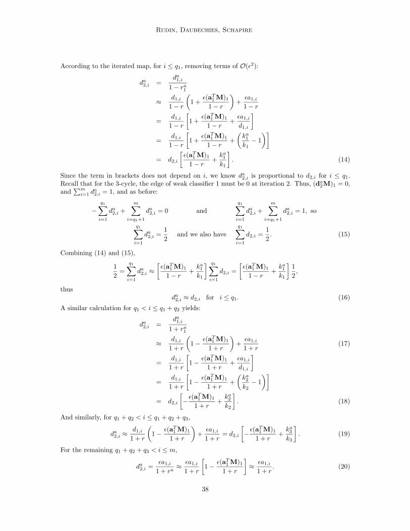
Rudin, Daubechies, Schapire
According to the iterated map, for i ≤ q1, removing terms of O(ε2):
da2,i =
da1,i
1 − ra1
≈ d1,i
1 − r
(1 +
ε(aT1 M)1
1 − r
)+
εa1,i
1 − r
=d1,i
1 − r
[1 +
ε(aT1 M)1
1 − r+
εa1,i
d1,i
]
=d1,i
1 − r
[1 +
ε(aT1 M)1
1 − r+
(ka1
k1− 1
)]
= d2,i
[ε(aT
1 M)11 − r
+ka1
k1
]. (14)
Since the term in brackets does not depend on i, we know da2,i is proportional to d2,i for i ≤ q1.
Recall that for the 3-cycle, the edge of weak classifier 1 must be 0 at iteration 2. Thus, (da2M)1 = 0,
and∑m
i=1 da2,i = 1, and as before:
−q1∑
i=1
da2,i +
m∑
i=q1+1
da2,i = 0 and
q1∑
i=1
da2,i +
m∑
i=q1+1
da2,i = 1, so
q1∑
i=1
da2,i =
1
2and we also have
q1∑
i=1
d2,i =1
2. (15)
Combining (14) and (15),
1
2=
q1∑
i=1
da2,i ≈
[ε(aT
1 M)11 − r
+ka1
k1
] q1∑
i=1
d2,i =
[ε(aT
1 M)11 − r
+ka1
k1
]1
2,
thusda2,i ≈ d2,i for i ≤ q1. (16)
A similar calculation for q1 < i ≤ q1 + q2 yields:
da2,i =
da1,i
1 + ra1
≈ d1,i
1 + r
(1 − ε(aT
1 M)11 + r
)+
εa1,i
1 + r(17)
=d1,i
1 + r
[1 − ε(aT
1 M)11 + r
+εa1,i
d1,i
]
=d1,i
1 + r
[1 − ε(aT
1 M)11 + r
+
(ka2
k2− 1
)]
= d2,i
[−ε(aT
1 M)11 + r
+ka2
k2
]. (18)
And similarly, for q1 + q2 < i ≤ q1 + q2 + q3,
da2,i ≈
d1,i
1 + r
(1 − ε(aT
1 M)11 + r
)+
εa1,i
1 + r= d2,i
[−ε(aT
1 M)11 + r
+ka3
k3
]. (19)
For the remaining q1 + q2 + q3 < i ≤ m,
da2,i =
εa1,i
1 + ra≈ εa1,i
1 + r
[1 − ε(aT
1 M)11 + r
]≈ εa1,i
1 + r. (20)
38

The Dynamics of AdaBoost
This last set of components will always shrink as t increases, since the last q4 examples are alwayscorrectly classified. From (16), (18), (19), and (20), we can see that each of the first three sectionsof da
2 is proportional to the corresponding section of d2 to O(ε2), and that the last section of da2 is
vanishing.Now calculating the vector a2 to O(ε), incorporating equations (16), (17), (19), and (20):
εa2,i = da2,i − d2,i ≈
0 if i ≤ q1
− εd1,i(aT1M)1
(1+r)2 +εa1,i
1+rif q1 < i ≤ q1 + q2 + q3
εa1,i
1+rotherwise
.
We will now show that a1 undergoes a contraction via the iterated map.
ε‖a2‖1 = ‖da2 − d2‖1 ≤ ε
(∑mi=q1+1 d1,i
)|(aT
1 M)1|(1 + r)2
+‖a‖1
1 + r
+ O(ε2)
≤ ε
(∑mi=q1+1 d1,i
)‖a1‖1
(1 + r)2+
‖a1‖1
1 + r
+ O(ε2).
Aside, we note(∑m
i=q1+1 d1,i
)= 1/2 + (
√5 − 1)/4 = (
√5 + 1)/4. Also, r = (
√5 − 1)/2, so
1/(1 + r) = (√
5 − 1)/2. Now,
‖a2‖1 ≤ ‖a1‖1
[1 +
√5
4
(√
5 − 1)2
4+
√5 − 1
2
]+ O(ε)
= ‖a1‖13(√
5 − 1)
4+ O(ε) < ‖a1‖1.
Thus, we have shown a contraction at the first iteration. The same calculation (with indices changedaccordingly) is valid for each iteration, since the relation between da
2 and d2 is now the same as therelation between da
1 and d1, that is, each section of da2 is proportional to the corresponding section
of d2 from (16), (18), and (19) (and the last section vanishes). Since the calculation is valid for eachiteration, there is a contraction to the manifold at every iteration. Hence, the manifold is stable.
Appendix C. 4 Cycle for the 3×3 matrix in the Non-Optimal Case
In this appendix, we prove the following theorem:
Theorem 8 For the 3×3 matrix analyzed in Section 4, AdaBoost in the non-optimal case mayproduce a 4-cycle which yields a maximum margin solution.
Proof We will show the existence of such a 4-cycle by presenting its coordinates, and omit a proofof stability. One coordinate on the cycle is given by:
dcyc1 =
(1
2,1
2−
√2
4,
√2
4
)T
.
The only choice for j1 is j1 = 2, and the edge value is (dcycT1 M)2 = 1/
√2, which is larger than 1/3.
Now, we compute dcyc2 using the iterated map:
dcyc2 =
(1
2 +√
2,1
2,
1√2− 1
2
)T
.
39

Rudin, Daubechies, Schapire
We now choose j2 = 1 even though it is not the optimal choice. We are justified in this choice, sincethe edge is (dcycT
2 M)1 =√
2 − 1 > 1/3. Now iterating again, we obtain dcyc3 :
dcyc3 =
(1
2,
√2
4,1
2−
√2
4
)T
.
Again, we must choose j3 = 3 since it is the only permissible edge, (dcycT3 M)3 = 1/
√2. Iterating,
dcyc4 =
(1
2 +√
2,
1√2− 1
2,1
2
)T
.
With the choice j4 = 1, the edge value is (dcycT4 M)1 =
√2 − 1 > 1/3, and the next iterate of the
map will yield dcyc1 . We have completed the proof.
40