The Division of Labor, Specialization, and Uncertainty

Catherine G. Barrera∗

Johnson School of Management, Cornell University

This Version: October 14, 2014

Abstract

While all sectors of the economy exhibit a division of labor, different industries share work

among groups in different ways. In particular, the rise of service industries has lead to a decrease

in specialization and an increase in job sharing. Two aspects of service industries set them apart

from manufacturing in this context: the inability to smooth production because services, unlike

goods, cannot be stocked, and uncertainty in the demand for different types of tasks. This paper

presents a model which shows that optimal division of labor, specialization, and team size in

an industry depend on the manifestation of these features in that industry, and can therefore

explain observed differences. The results demonstrate that uncertainty and the inability to

smooth production work together to reduce the division of labor by increasing the value of

generalists who move between tasks that are temporarily in high demand.

∗cbarrera@cornell.edu This paper is the third chapter of my dissertation. I would like to thank my advisors,Oliver Hart, Philippe Aghion, and Eric Van den Steen, for their insights and suggestions.

1 Introduction

Across all levels of society, production is characterized by the division of labor. Work is shared

between multiple individuals in households, in organizations, and in the economy, because through

specialization and trade productivity increases. However, productive activities are not shared

among groups in the same way everywhere.

For example, work on an assembly line is commonly broken down into small sets of tasks,

each of which is assigned to an individual, with no two individuals working on the same task.

Contrastingly, at a restaurant, several individuals do the same job or set of tasks (i.e. there

are multiple waiters), despite the ability to break the job down into smaller parts (i.e. taking

orders, serving food, printing and delivering checks) which would allow individuals to become more

specialized.

The particular way in which a given set of work is divided among a group depends on the

features of the production process involved. The contrast between manufacturing and services

highlights two specific features that impact specialization and the division of labor: uncertainty

over task flow or demand—the quantity and type of tasks required may be fixed or changing—

combined with the inability to smooth production—goods can be stocked while services must be

provided on demand.

This paper introduces a model of the division of labor in which specialization, job sharing,

and team design depend on the uncertainty of task availability in an environment where production

may be smoothed or not. The results of the model both replicate previous findings in the litera-

ture, reflecting the organization of work in manufacturing, and extend the analysis of gains from

specialization to explain differences in the division of labor across industries.

In the model, production occurs when a team of agents (possibly one agent) completes a

project composed of a variety of tasks. The productivity of the team depends on the proficiency

1

with which each task is completed (in this case project output is the minimum function). An agent

can become more proficient at a particular type of task by working on that type more often; there

are gains from specialization. Optimal division of labor incorporates team size and the assignment

of tasks to the agents in the team.

The model shows that when production is predictable—each project consists of the same set

of tasks—division of labor is maximized—no two agents work on the same task. However, when the

composition of projects is uncertain and production cannot be smoothed, specialization and the

division of labor decrease due to two effects. First, the inability to smooth production equates to

an inability to completely control the depth of specialization. When production can be smoothed,

any job, no matter how narrow, can fill an agent’s time allowing him to gain maximal proficiency.

If an agent can only practice a task when it is demanded (e.g. a hair stylist only gives a haircut

when a client requests one), then proficiency is limited by demand.

Second, fluctuations in the demands of different types of tasks increase the value of generalists

because these agents more effectively move to tasks that are momentarily in high demand. For

example, two waiters who both take orders and serve food are better equipped for occasions when

two customers arrive at their restaurant simultaneously than one waiter who specializes in taking

orders and one who specializes in serving food. In particular, though it is always possible for an idle

specialist to work on an overflow task outside his specialization, when overflow tasks are sufficiently

likely, two generalists (agents with moderate proficiency in this task type) will do better than two

specialists (one expert and one novice at this task type).

An alternative way of dealing with fluctuations in demand is to utilize additional agents.

Rather than moving a team of generalists between different types of tasks, each type of task could

be fielded by a team of agents dedicated to only that type, allowing for greater specialization. When

labor is divided in this way, instead of using spare time on tasks outside their specialization, these

2

agents sit idle. Thus, the model demonstrates that there is a tradeoff between specialization and

agent utilization.

This paper adds to the literature discussing specialization and the division of labor. In

this literature, increasing returns to specialization drive the division of labor, resulting in no two

individuals working on the same type of task (e.g. Rosen (1983), Stigler (1951)). This result has

conflated the concept of division of labor with team size and also with specialization; adding mem-

bers to a team implies that the set of all types of tasks is divided in to narrower specializations and

trade is increased. Suggested limits to the division of labor include the size of the market (Stigler,

1951) and communication costs (Becker and Murphy, 1992) and, in reference to job narrowness,

the flow of different types of tasks (Wadeson, 2013).

Research on organizational design and job design touches on similar topics. The literature on

information processing considers specialization, but due to communication costs no two agents work

on the same type of task (Bolton and Dewatripont, 1994). Garicano (2000) examines hierarchies

where at each level, an optimal number of agents works on a single job and the set of all tasks is

split among the different levels optimally; however, there are no gains from specialization in that

paper.

This paper shows that division of labor (the inverse of job sharing), specialization (the

narrowness of jobs), and team size can move separately. In particular, by incorporating the inability

to smooth production—which has not been considered in this context—the model allows for the

optimal division of labor to display job sharing even when there are gains from specialization. Thus,

the model enriches our understanding of the concepts of division of labor and specialization, and

it shows that the division of labor may be limited by the production technology or process.

The paper proceeds as follows: The next section sets up the model. Section 3 replicates

previous results, then examines the effects of deterministic and stochastic project availability on

3

specialization. Section 4 discusses the effect of task distribution on job overlap for when production

can and cannot be smoothed. The tradeoff between specialization and agent utilization is discussed

in Section 5. Section 6 concludes.

2 Model Setup

An agent is able to specialize, increasing his productivity on a particular type of task by spending

more time working on that type of task. Examples of this phenomenon abound, but this fact is

particularly salient to academics who specialize in narrow subfields. Specialization is facilitated by

the division of labor. When an agent does not need to produce each good and service himself, he

can use time that would otherwise be devoted to producing a wider variety of goods to develop

specialized skill.

2.1 Production

Suppose that tasks have equal productive potential, but are horizontally differentiated. Let Ω be

the set of task types, s. A project P is a set of tasks, with distribution over Ω, FP (s). Suppose that

all projects are the same size, and normalize |P | = 1. Assume that tasks require a fixed amount of

time to complete, which is identical for all tasks; then in some sense the size of P measures both the

number of tasks in it and the number of man-hours required to complete the project. Therefore,

say a project takes one unit of agent-time to complete. Assume each task is continuously divisible

so a project can be divided between any number of agents.

Let τi,s be the frequency with which an agent, i, works on task type s ∈ Ω. His productivity

from working on any task of type s is E(τi,s). There are decreasing returns to practice, so E′ > 0

and E′′ < 0. Let AP,s be the set of agents who work on type s tasks in project P . Project

production is a function of the productivity on each task in the project. Following Becker and

4

Murphy (1992), assume production is determined by the minimum performance on a task in the

project. Production on project P is given by

Y (P ) = mins∈P

[mini∈AP,s

E(τi,s)

]

Becker and Murphy (1992) argue that for a productive activity that requires all tasks to

complete, the production function will be the minimum function. Their argument focuses on on

goods and interprets Y as quantity produced; however, this production function also applies to

quality, which is a more natural interpretation when considering productive value on a project of

fixed size, as modeled here.

The output quality interpretation can be applied to goods; a product is sometimes only as

good as its lowest quality part. Moreover, quality may be a better measure of productive value than

quantity for the provision of services. For example, the value of customer service is in customer

retention which depends on quality. One bad experience can cause a customer to switch brands,

so the minimum quality of service is essential in determining productive value.

3 Limits to Specialization

3.1 Specialization Limited by the Extent of the Market

This model can be used to replicate the result from Becker and Murphy (1992), based on Smith’s

(1776) argument, that the division of labor is limited by the extent of the market. Let Ω = [0, 1] so

there is no limit to how narrow an agent’s area of expertise can be. Assume all projects are identical.

Let FP be uniform on Ω. Further, suppose that the availability of projects is unlimited, so that as

soon as one project is completed another can begin. This assumption applies well to industries like

5

manufacturing of consumer goods or research production; as noted in the introduction, it is always

possible to produce an additional pin or an additional paper.

An agent who works on a project alone divides his time evenly among all tasks, which in

this case is the same as dividing time evenly among task types due to the uniform distribution.

Thus, the agent will do one task of each type (fP (s) = 1 ∀s) during each period, τs = 1 for all s.

The production of this agent will be

E(1)

Suppose an agent works on m projects in a unit of time. Without loss of generality1 denote the set

of tasks he completes for project j, [sj , sj ]. The time constraint for this agent is

m∑j=1

(sj − sj) = 1

An agent’s proficiency on a type of task, s, is a function of the number of these m projects for

which this type of task is in the agent’s task set. Define a binary variable δj,s = 1 when s ∈ [sj , sj ]

and 0 otherwise. Then

τs =m∑j=1

δj,s

A team of n agents can complete up to n projects each period. The maximum possible

output on a singe project is

E(n)

because if τi,s > n for some agent i and task type s, then τi,s′ < n for some s′ 6= s, otherwise i’s time

constraint is violated. This maximum is achievable on all n projects by setting [si,j , si,j ] = [ i−1n , in ]

for agents i ∈ [1, n]. The optimal task assignment for a team of n agents divides the set of task

1All tasks have equal value and are equally likely; therefore tasks can be relabeled so that each agent’s job is acontinuous set.

6

types into n non-overlapping jobs of equal size. Then the per unit time output of n agents is

nE(n)

The productivity of each agent in a team increases with the team size. Thus, splitting any team

into smaller units, reduces total productivity. When interpreting a project the set of productive

tasks done by a society, following the ideas of Adam Smith, the optimal team includes all agents

in the market, denoted N .

Becker and Murphy (1992) argue that this result shows that the division of labor is limited

by the extent of the market. While it is true that specialization here is increasing in the number of

agents and is only limited by the total number of agents in the market, in a sense labor is equally

divided for all n because no two agents work on the same task type for any size team.

3.2 Specialization Limited by the Availability of Projects

The assumption that the number of projects is unlimited allows any size specialization to fill an

agent’s time, which gives the agent the practice required to improve proficiency. Assume instead

that the number of tasks available in a given period is limited. Limits to the amount of work

available are typical in service industries. Customer service representatives, hair stylists, and dry

cleaners (to name a few) can only provide their services when a customer requests them.

Suppose that the number of projects available in a unit of time is M < N . Then M agents

can complete the available work during that time. Maximum production is achieved by partitioning

Ω into M subsets, [si, si], with M |[si, si]| ≤ 1. The depth of specialization is clearly limited by

the number of tasks available. Increasing the size of the team beyond M agents, while supported

by market size, can narrow each agent’s specialization but cannot deepen the specialization, and

therefore cannot increase output. Further, if there is any other activity with value ε > 0 that agents

7

can participate in, including leisure, the size of the team, as well as the narrowness of specialization

is strictly limited by the volume of projects available.

3.3 Uncertainty over Project Limits

When project availability is limited, it is usually also uncertain. Demand for services may be

cyclical or fluctuate unpredictably. Rather than assisting twenty customers each day, a customer

service department may help five one day and thirty the next.

Note that under uncertainty an agent’s proficiency will depend on the realization of the

random variable over time. The following analysis uses average frequency to determine an agent’s

proficiency. This notion of proficiency is advantageous for two reasons. First, for a long horizon,

any realization of the random variables will have the same average. Furthermore, as opposed to a

discounting function, with a long horizon, the average frequency does not fluctuate with fluctuations

in work volume2.

Assume that in a unit of time, there are m ∈ R projects available. (A continuous approxi-

mation will simplify the notation and calculations.) Let G(m) be the distribution over this number

of projects. Suppose a team consists of n agents, then for all m ≥ n, the job design problem is

like that when the availability of projects is unlimited. In these cases, the optimal division would

be n jobs of equal size. For m < n, the limit of task availability is binding, fixing productivity

at mE(m); however, in these cases, dividing projects into m+ k equal size jobs does not decrease

productivity for any k.

Therefore, the optimal division will be to assign each of the n agents an equal size subset of

task types. For example

[si, si] =

[i− 1

n,i

n

]2This analysis, then, focuses on long-term job and team design. The results also hold for a two period model in

which proficiency is gained in the first period and used for production in the second. A two period example is givenin the Appendix to illustrate that the same forces drive optimal job design.

8

for 1 ≤ i ≤ n. For all m, each agent does his subset of each of the m projects available. For each

agent i in the team, the team works on an ith task whenever m ≥ i. Therefore,

τs =

∫ n

01−G(x)dx

and total output is given by

(∫ n

01−G(x)dx

)E

(∫ n

01−G(x)dx

)

3.3.1 Team Size and Uncertainty

The previous two subsections have identified the optimal team size in two extreme cases: When

there is certainty over the number of projects and this number is limited below the total number

of agents, the optimal team size is equal to the number of projects available. On the other hand,

when the probability that the number of projects available exceeds the number of agents goes to

1, the optimal team size is the total number of agents in the market.

These two cases suggest that optimal team size is a function of the distribution of task

availability, G(m). Indeed, the optimal team size is increasing in mean of this distribution. Some

distributions can be ranked in terms of uncertainty, for example, when one is a mean preserving

spread of another. In addition to increasing in the mean of G(m), team size is increasing in

uncertainty for a refinement of mean preserving spreads.

The output function in terms of n derived in early sections is weakly increasing in n. Suppose

now that there is a cost to adding agents to a team C(n), with C ′ > 0 and C ′′ ≥ 0. A brief discussion

of possible cost functions and interpretations is given below, but for now assume that this function

9

is such that there is an internal solution to the optimal team size problem.

maxn

(∫ n

01−G(x)dx

)E

(∫ n

01−G(x)dx

)− C(n)

It will help to pick a specific proficiency function E; following Becker and Murphy (1992) again,

let E(x) = xθ with θ ∈ (0, 1). Then the first order condition of the optimization problem is

(1 + θ)

(∫ n

01−G(x)dx

)θ(1−G(n))− C ′(n) = 0

For an internal solution to exist, the first term must be decreasing in n. This fact combined with

the fact that C ′′ ≥ 0 indicates a condition for the optimal team size to be increasing. Denoting the

optimal team size nk when the distribution is Gk, it must be that n2 > n1 when

(1 + θ)

(∫ n

01−G2(x)dx

)θ(1−G2(n)) > (1 + θ)

(∫ n

01−G1(x)dx

)θ(1−G1(n)) (1)

at n = n1.

It is plain, then, that n2 > n1 whenG2 first order stochastic dominatesG1, because inequality

(1) holds for all n. When there is a higher probability of more projects being available, the optimal

team has more members. More interestingly, a mean preserving spread can also lead to an increase

in the optimal team size. In this way, optimal team size is increasing in uncertainty, for a given

expected number of projects.

Let Gr(m) be a distribution on the number of projects available, and let Gr+1 be a mean-

preserving spread of Gr.

10

Claim 1. There is a probability (1 − G∗r) ∈(

(1−Gr(nr)), (1−Gr(nr))1

1+θ

)such that nr+1 ≥ nr

if and only if

(1−Gr+1(nr)) ≥ (1−G∗r) (2)

Proof. See Appendix.

A mean preserving spread satisfying inequality (3) places more weight on higher project limit

values. Then a mean preserving spread of Gr with a sufficiently thicker right tail above the optimal

team size for Gr has a larger optimal team size than Gr. When uncertainty over the number of

projects available increases in a way that puts sufficiently more weight on the number of projects

exceeding the optimal team size, the team size increases. even when the mean number of projects

remains the same.

Observation. Any mean preserving spread of a distribution with no uncertainty increases optimal

team size.

This is because (1 − Gr(n∗r)) = 0 for a distribution in which all weight is on n∗r , and (1 −

Gr+1(n∗r)) > 0 for any mean preserving spread of Gr.

3.4 Costs to Increasing Team Size

Elsewhere in the literature regarding division of labor, specialization, and team size, coordination

and communication costs are suggested as limits to team size (Becker and Murphy, 1992; Bolton

and Dewatripont, 1994). The functional form of these costs is considered to be convex. Another

possibility is that there are outside activities, like leisure, that provide a private value that cannot

be traded. In this case, the cost function would be linear in team size.

This type of cost function has not been a focus in the past because an internal solution to the

team size problem with linear cost is only possible if the production function is concave in team size,

11

while the production functions considered display increasing returns to scale (team size), or gains

from specialization. When uncertainty over the number of available projects is introduced, however,

a production function with gains from specialization may be concave in team size, depending on the

shape of the distribution of demand. Thus, it is possible for team size to be limited by uncertainty,

in a setting where communication or coordination costs are minimal.

4 Limits to the Division of Labor

4.1 Task Sharing under Predictable Production

The result that the set of task types is divided into equal-sized non-overlapping jobs rests on the

assumption that all projects are uniformly distributed over all possible task types, Ω. It may not be

the case that the optimal specialization requires a partition of the set of task types into n subsets for

n agents. Joint production is not always maximized with a division of labor and trade. Even with

unlimited divisibility of task types, some agents may share a specialization because proportionally

more of some tasks are required for project completion.

Assume again that all projects are identical and that there is unlimited availability of

projects. Let the density of task types in a project be the piecewise function:

f(s) =

23 if s ∈ [0, 12 ]

43 if s ∈ (12 , 1]

Then a team of n agents can complete n projects in one period. The maximum proficiency that can

decide project output is E(τs) = (E 23n); that is the maximum output on a project is the maximum

proficiency with which an agent can do the least frequent type of task. For every one task of type

s ∈ [0, 12 ], there are two of type s′ = s+ 12 . Thus, if an agent completes all tasks of type s′ ∈ (12 , 1],

12

the proficiency on this task type is E(43n), while total production will remain

nE

(2

3n

)

because performance on less frequent tasks cannot be increased. Therefore, the following two task

allocations, both of which divide the project into n equally sized jobs, achieve maximum output3.

Task types s ∈ [0, 12 ] are divided into equal segments, with no two agents working on the same type

in this region. One allocation would divide the task types s ∈ (12 , 1] in a similar way, with no over

overlapping jobs, but with smaller segments for each agent than in the range [0, 12). That is, for

each agent, i ∈ [1, n]

[si, si] =

[1

2

i− 1

n,1

2

i

n

]+

[1

2+

1

2

i− 1

n,1

2+

1

2

i

n

]

The other optimal allocation divides task types in s ∈ (12 , 1] into larger jobs that are then shared

by two agents:

[si, si] =

[1

2

i− 1

n,1

2

i

n

]+

[1

2+j − 1

n,1

2+j

n

]

with

j =

i+12 if i odd

i2 if i even

for i ∈ [1, n].

The example shows that for high volume tasks, it can be equally productive to have multiple

agents share the same specialty as it would be to have them divide that specially, becoming even

more proficient in a smaller set of task types. In this case, the result is due to the fact that lower

volume tasks cannot support the same level of specialization, so the gains from further dividing labor

3In this example n may be the maximum number of agents or the maximum number to tasks, depending whichis the limiting factor.

13

on high value tasks cannot be realized. However, this is an important case to consider because it has

implications for when project distributions over task types vary. In fact, it may be that overlapping

jobs are strictly better than a complete division of labor because there is uncertainty over which

task types will be high frequency.

4.2 Task Sharing under Project Uncertainty

To illustrate this point, consider a simple example of the model. Suppose that there are two task

types, Ω = A,B. Further suppose that the number of projects is limited, but there are two

projects with certainty. Finally, suppose that each project consists entirely of one of the task types.

There is a probability, pA of there being two projects of type A tasks, a probability pB of there

being two projects of type B tasks and a (1− pA − pB) of there being one project of each type.

First suppose the team consists of two agents. Then when both projects are the same, each

agent will work on one of them. The only question is how to divide the work on two different

projects. Let γi,s be agent i’s share of the project containing only s type tasks. Then, agent i’s

frequency of working on s is

τi,s = ps + (1− ps − ps′)γi,s

Note that,∑iγi,s = 1 and

∑sγi,s = 1, so γi,s = γi′,s′ = γ. Thus, there is only one choice parameter to

optimize output. Because the production function is the minimum function, output is discontinuous

at γ = 0. Further, because the two agents have the same potential for productivity, the domain of

14

output can be limited to γ ∈ [0, 12 ].

E[Y (γ = 0)] =

pA[E(pA) + E(1− pB)]

+ (1− pA − pB)[E(1− pB) + E(1− pA)]

+ pB [E(pB) + E(1− pA)]

E[Y (γ 6= 0)] =

pA[E(pA + (1− pA − pB)γ) + E(pA + (1− pA − pB)(1− γ))]

+ (1− pA − pB)[E(pA + (1− pA − pB)γ) + E(pB + (1− pA − pB)γ)]

+ pB [E(pB + (1− pa − pb)(1− γ)) + E(pB + (1− pa − pb)γ)]

For γ 6= 0, E[Y (γ)] is increasing in γ. Thus, optimal task sharing is either γ = 0 or γ = 12 .

In either state where both projects are the same, γ = 12 does better for all pA and pB because E(τ)

is concave. When pA = pB = 0, the optimum is at γ = 0; when there is always one task of each

type, each agent specializes in one type of task. However, as pA and pB increase, the performance

of specialization decreases in the state where the two projects are different, because each agent

must spend some time on the other type of task. Thus, the division of labor is decreasing in pA

and in pB.

A larger team would weaken the constraints in this optimization problem, allowing for the

sharing of type A tasks to vary independently of the sharing of type B tasks; γi,A 6= γi′,B. Although

each task type may support the work of two agents, a three agent team always dominates a team

15

of four agents. When two agents share work on a task type, they must share it equally. Therefore,

if it is optimal for each task type to be shared, the same two agents can share both task types.

Three agents perform better than two only when γs = 0 is optimal for one of the task types

but not the other. In this case, the time constraints cannot be satisfied with only two agents. One

agent is required to work on a project of type A (for example) whenever such a project is available,

but two agents should share the single B type project when there is one of each type. With

only two agents, one agent would be required to work on one and a half projects with probability

(1− pA − pB).

While the distribution over the number of projects for each task may be such that the

optimal team size is two agents, combining these task types so one team works on both types is at

least as efficient because an agent on team A can work on a type B task when he is not working on

a type A task. Because the quantity of different task types do not fluctuate together, job sharing

is possible, and job sharing allows for the same output to be achieved with a smaller number of

agents.

This argument elucidates the role of a constant project limit in demonstrating the optimality

of job sharing in this example. The next section discusses optimal job sharing when the volume of

different task types can vary freely. First, a brief illustration will show that the job sharing with

constant project limit result does not depend on a finite number of task types.

Consider a team of n agents, and assume that the number of projects in a unit of time is also

n. Suppose all n projects in a given period are identical, but projects may be distributed over the

set of task types, Ω = [0, 1], in a number of ways. Specifically, assume that there is a probability

p that the tasks in each project are distributed uniformly, and there is a (1 − p) probability that

half of the task types are twice as likely as the rest (as in Section 4.1) and that every possible

16

subset S ⊂ Ω with |S| = 12 can be weighted this way. (The particular probability distribution over

potential projects is not essential to this illustration.)

As outlined in Section 3.1, the optimal division of labor when the project’s distribution over

tasks is uniform is a partition of Ω = [0, 1] into n equal sized subsets. In some states this division

of labor is not feasible because if agents are limited to working only on tasks inside this specialty,

the time constraint of some agents will be violated—they will not be able to complete all tasks in

their specialty.

In particular, there will be some state in which all of agent i’s tasks are given higher weight.

Recalling the distribution

f(s) =

23 if s 6∈ S

43 if s ∈ S

Agent i’s segment of task types will require

n4

3

1

n> 1

units of time to complete. Thus, no partition of Ω into n equal subsets is a feasible division of labor

in this case. In fact, no partition of Ω into n sets is feasible. Instead, Ω can be partitioned into

n2 subsets, with each subset being shared by two agents. Then for any realization of the task type

distribution, there will be a sufficient number of agents to complete each task type when agents

only work on tasks within their specialization. In this case, agents are less specialized, and labor is

less divided. As the volatility of project distributions increases (i.e. the maximum volume of each

task type increases), the division of labor decreases—more agents share a specialization.

When the volume of a particular task type fluctuates, more agents will be required to work

on that type of task in some states than are required in other states. Then, there is a positive

17

probability that an additional agent will spend some time working on that task type. Maximizing

gains from practice for one agent comes at the cost of less proficient agents sometimes working on

that type of task. Reducing the division of labor, by creating overlapping jobs, allows all agents

who work on a particular type of task to do so with a moderate level of proficiency. When there

is a sufficiently high probability of there being excess tasks, a team of moderate proficiency agents

will perform better than a team with some experts and some novices.

5 Job and Team Design: Varying Task Type and Project Quantity

The assumptions used in the previous sections have required that task types be related to each

other in particular ways, either always co-occurring because there is a fixed task type distribution

(Section 3) or being negatively correlated because there is a fixed project limit (Section 4). In some

industries the availability of different task types may be related in other ways (or may even be

independent). This section uses a simple example of the model to discuss the impact of weakening

the assumptions used above on optimal job design and team size.

Suppose that there are four task types (Ω = A,B,C,D), and that each project consists

entirely of a single task type. Further suppose that for each task type, in a unit of time, up to one

project may be available; let ps be the probability that a project of type s is available. Finally,

suppose there is a value to leisure that is ω. Then if the assignment of agents to tasks is done for

each type individually, an agent would be assigned to task type s when psE(ps) ≥ ω.

The optimal overall job design and team size depend on the joint distribution of project

availability. To illustrate the relationship between distribution and optimal team design, the fixed

task type and the fixed project limit distribution examples of this setup will be considered before

discussing more general distributions.

18

5.1 Fixed Task Type Distribution

Suppose that Pr[ s′ | s ] = 1 for all s′ and s ∈ Ω; task types are co-occurring. There is a fixed

distribution over task types; namely, in each state, each task type represents a quarter of all

projects. It must be that ps = p for all s ∈ Ω and that there are always either four projects or

none.

In this case, the team size is the sum of the individually optimal teams. If and only if

psE(ps) ≥ ω for some s ∈ Ω, psE(ps) ≥ ω for all s ∈ Ω. Optimally, there is no job overlap in

this case because if two agents share two task types, the performance on those task type’s projects

decreases. Thus, the optimal combined team for all task types has the same size and job design as

the optimal separate teams for each task type.

5.2 Fixed Project Limit with Negative Correlation

At the other extreme, assume that there is always one project, so that Pr[ s′ | s ] = 0 for each

s′, s ∈ Ω. Then one agent always does at least as well as a larger team, because maximum production

of a task type s is psE(ps), and one agent can achieve this level of production for all task types.

Thus, rather than separating different task types, it is always better to combine them into a single

team; division of labor is at a minimum.

Note that if it is optimal for an individual task type to be done separately, then that task

type will be done in the combined team: If ps′E(ps′) ≥ ω for some s′, then∑spsE(ps) ≥ ω. In

addition, some task types that would not be done individually may be done in the combined team

because spare time can be used for tasks that are not frequent enough to command their own team.

Thus, the combined team never does worse than individual teams, and it performs strictly better

than individual teams whenever∑spsE(ps) ≥ ω, because more projects are done, sometimes with

fewer agents.

19

5.3 Illustration of Other Distributions

In general the number of projects available could be anywhere between zero and four. Suppose the

probability of two projects being available is near one, and that each combination of two projects

is equally likely.

Consider a team of two agents. This team must have some job overlap because for any two

mutually exclusive subsets of Ω, there is some probability that both available task types are in one

of those subsets. Thus, there is at least one task type for which two agents share responsibility,

and the performance of this task type could be increased by assigning all projects of this type to a

single agent. Increasing proficiency in this way can only be achieved by increasing the team size.

With a team of four agents, for example, each project could be done with maximum productivity,

psE(ps).

Suppose that there are never more than two projects. Then increasing the team size above

two does not increase the number of projects that are done. Thus, when the probability of three

or four projects is sufficiently low, increasing the team size increases the productivity with which

projects are done, but it decreases the utilization of agent time. That is, each task type can become

more specialized because an agent is able to spend more of his time on only that task type, but the

agent also spends more time idle, as he does not use his spare time to work on other types of tasks.

Thus there is a tradeoff between specialization and efficiency of agent time. Division of

labor and specialization are increased by increasing the number of agents. However, under limited

workflow and uncertainty over task types, the gains from adding agents to the team are constrained

because the probability that an agent is idle increases and because specialization is limited by the

availability of tasks within a narrow field.

20

6 Conclusion

The division of labor is a concept fundamental to the study of economics. It has important im-

plications across the economy, but especially for job and team design. Intuitively, the particular

way in which labor is divided should depend on the nature of the work being done. However, the

existing literature hasn’t addressed the relationship between workflow and the division of labor.

During the last century, production in post-industrial economies has shifted away from man-

ufacturing industries towards service and technology industries. The workflow in these industries

differs greatly from that in manufacturing, implying observed patterns in the division of labor

should be expected to change. In order to better understand these changes, our theories must be

adapted to reflect non-manufacturing industries.

The model presented in this paper illustrates the impact of uncertain workflows on job and

team design. It shows that proficiency from specialization may be limited by the availability of

tasks. In addition, as uncertainty over the distribution of task types increases, specialization and

the division of labor both decrease, because the ability to move agents between different types of

tasks becomes more important. Finally, uncertain workload can lead to an increase in team size;

this increase in size may allow for a greater division of labor, but can also result in decreased agent

utilization.

In addition to elucidating the relationship between shifts in the economy and changes in

division of labor, job design, and team design, this model has cross-sectional implications. It

suggests that differences in division of labor and specialization across industries may be attributable

to differences in the nature and uncertainty of the work in those industries. Furthermore, it

indicates that within an industry, some tasks are more likely to be shared among groups than others;

therefore, some tasks will have a lower degree of specialization than others. In this way it connects

21

differences in job design and specialization (for example between faculty and administrators) with

differences in the nature of work (research generation versus service provision).

22

References

Gary Becker and Kevin M. Murphy. The divisoin of labor, coordination costs, and knowledge. The

Quarterly Journal of Economics, 107(4):1138–1160, 1992.

Patrick Bolton and Mathias Dewatripont. The firm as a communication network. The Quarterly

Journal of Economics, 109(4):809–839, November 1994.

Luis Garicano. Hierarchies and the organization of knowledge in production. Journal of Political

Economy, 108:874–904, 2000.

Sherwin Rosen. Specialization and human captial. Journal of Labor Economics, 1(1):43–49, 1983.

Adam Smith. An Inquiry into the Nature and Causes of the Wealth of Nations. 1776.

George J. Stigler. The division of labor is limited by the extent of the market. Journal of Political

Economy, 59(3):185–193, 1951.

Nigel Wadeson. The division of labour under uncertainty. Journal of Institutional and Theoretical

Economics, 169(2):253–274, 2013.

23

A Mathematical Appendix

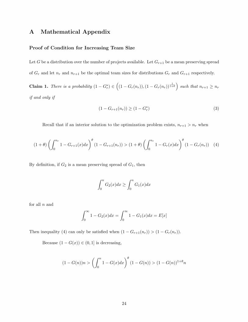
Proof of Condition for Increasing Team Size

Let G be a distribution over the number of projects available. Let Gr+1 be a mean preserving spread

of Gr and let nr and nr+1 be the optimal team sizes for distributions Gr and Gr+1 respectively.

Claim 1. There is a probability (1 − G∗r) ∈(

(1−Gr(nr)), (1−Gr(nr))1

1+θ

)such that nr+1 ≥ nr

if and only if

(1−Gr+1(nr)) ≥ (1−G∗r) (3)

Recall that if an interior solution to the optimization problem exists, nr+1 > nr when

(1 + θ)

(∫ nr

01−Gr+1(x)dx

)θ(1−Gr+1(nr)) > (1 + θ)

(∫ nr

01−Gr(x)dx

)θ(1−Gr(nr)) (4)

By definition, if G2 is a mean preserving spread of G1, then

∫ n

0G2(x)dx ≥

∫ n

0G1(x)dx

for all n and ∫ ∞0

1−G2(x)dx =

∫ ∞0

1−G1(x)dx = E[x]

Then inequality (4) can only be satisfied when (1−Gr+1(nr)) > (1−Gr(nr)).

Because (1−G(x)) ∈ (0, 1] is decreasing,

(1−G(n))n >

(∫ n

01−G(x)dx

)θ(1−G(n)) > (1−G(n))1+θn

24

for all n and all G. Thus, if (1−Gr+1(nr))1+θ = (1−Gr(nr)),

(∫ nr

01−Gr+1(x)dx

)θ(1−Gr+1(nr)) >

(1−Gr+1(nr))1+θnr = (1−Gr(nr))nr

>

(∫ nr

01−Gr(x)dx

)θ(1−Gr(nr))

Thus, Inequality 4 holds at (1 − Gr+1(nr)) = (1 − Gr(nr))1

1+θ . Then there is a (1 − G∗r) <

(1 − Gr(nr))1

1+θ such that if (1 − Gr+1(nr)) = (1 − G∗r) the inequality holds with equality. Then

whenever (1−Gr+1(nr)) ≥ (1−G∗r) the inequality must hold. Because the inequality cannot hold

for (1−Gr(nr)) = (1−Gr(nr)), it must be that (1−G∗r) ∈(

(1−Gr(nr)), (1−Gr(nr))1

1+θ

).

Two Period Example

This section considers job design under uncertainty over task type distribution in the short-run.

Consider a two period model in which agents accrue proficiency only after completing work. Then

agents work to accrue skill in the first period, and work to produce output in the second period.

Following the example given in Section 4.2: Suppose that there are two task types, Ω =

A,B. Further suppose that the number of projects is limited, but there are two projects with

certainty. Finally, suppose that each project consists entirely of one of the task types. There is

a probability, pA of there being two projects of type A tasks, a probability pB of there being two

projects of type B tasks and a (1− pA − pB) of there being one project of each type.

25

Job design is only relevant when there is one project of each type in the first period. Each

project could be assigned to one agent, in which case Period 2 output would be:

pA[E(1) + E(0)]

+ (1− pA − pB)[E(1) + E(1)]

+ pB [E(0) + E(1)]

Alternatively, each project could be split between the two agents. Let γ ∈ (0, 12 ] be the

smaller share of a project, noting that γ when the team consists of two agents. In this case, output

is given by:

pA[E(1− γ) + E(γ)]

+ (1− pA − pB)[E(1− γ) + E(1− γ)]

+ pB [E(γ) + E(1− γ)]

The derivative of this expression with respect to γ is

(pA + pB)E′(γ)− (2− pA − pB)E′(1− γ)

Because E is concave, E′(γ) ≥ E′(1−γ) on the domain of γ. Then, for a sufficiently large (pA+pB),

the optimal γ is positive, and the optimum goes to 12 as (pA + pB) goes to 1. When the probability

of there being excess tasks of a single type increases, it is more important for both agents to have

some proficiency in each type of task.

26

The difference between this example and the one given in the text is that here in Period

2 when there is one project of each type, they are not shared between the agents. Sharing tasks

in the last period of a finite model decreases output because the minimum proficiency applied to

each project decreases. There is also no benefit to sharing the projects because there are no future

projects.

In a finite model with more periods, project sharing in intermediate periods will contribute

to agent’s performance in subsequent periods, even though it decreases current performance. These

intermediate periods are similar, then, to the analysis in the text. When there are more than two

periods, project sharing in the first period becomes even more valuable because it increases the

performance on future shared projects. Taking this added benefit to its extreme, a very long time

horizon, optimal task sharing must be γ = 12 , as shown in the text.

27