The Distribution of Risk Aversion∗

Gurdip Bakshia† Dilip Madanb‡

aSmith School of Business, University of Maryland, College Park, MD 20742, USA

b Smith School of Business, University of Maryland, College Park, MD 20742, USA

(First draft November 2005; this version November 18, 2006)

Abstract

This paper develops a framework for deriving and inferring the distribution of relative risk aversionfrom financial markets. The theoretical constructions (i) rely on a fairly robust form of aggregating themarginal rate of substitution of individuals that are either long or short the market-index, and (ii) specifiesa positive measure for the risk aversion coefficient capturing the feature that a proportion of the populationpossesses a distinct risk aversion. The implementation of the theoretical model reveals substantial hetero-geneity in the coefficient of relative risk aversion. Our empirical approach supports the competitive marketsparadigm that enforces positive skewness in the risk aversion distribution. The evidence also points to thepresence of a risk aversion distribution that is characterized by heavy tails. We discuss the asset pricingimplications of theory and empirical findings.

JEL CLASSIFICATION CODES: G0, G10, G11, G12, G13, C5.

∗We thank Doron Avramov, Nick Bollen, Markus Brunnermeier, Steve Heston, Nengjiu Ju, Pete Kyle, Mark Loewenstein,Ron Masulis, Steven Ott, Matt Pritsker, Georgios Skoulakis, Hans Stoll, Joel Vanden, Greg Willard, Liuren Wu, and Hao Zhou forconstructive discussions. We are grateful to George Constantinides for helping us clarify a crucial step. The seminar participantsat University of North Carolina-Charlotte, University of Maryland, and Vanderbilt University provided useful suggestions. Wewelcome comments, including references to related papers we have inadvertently overlooked. The research assistance of ShevenduDang, Carl Ullrich, and Yue Xiao is gratefully acknowledged.

†Tel.: +1-301-405-2261; fax: +1-301-405-0359. E-mail address: gbakshi@rhsmith.umd.edu.‡Tel.: +1-301-405-2127; fax: +1-301-405-0359. E-mail address: dbm@rhsmith.umd.edu.

1. Introduction

What is the empirical distribution of risk aversion in competitive markets where risks are traded? How

relevant is heterogeneity in risk aversion for modeling the pricing distributions of the market-index that

drive index option markets? What are the analytical building blocks for aggregating marginal utilities

when a source of heterogeneity is risk aversion and when one recognizes that agents can hold both long

and short positions in the market-index? How severe is the constant risk aversion restriction in empirical

tests of representative agent pricing models? The intent of this research is to show how these questions can

be answered in a theoretical framework that synthesizes the role of distributional properties of risk aversion

in the aggregate marginal utility, and hence in the pricing distributions of the market-index. The theoretical

model provides the impetus for estimating the distribution of risk aversion in the population from financial

market data.1

Our approach relies on a number of assumptions. First, there are two classes of investors that respec-

tively take either a long-position or a short-position in the equity market-index, the source of which can

be heterogeneity in expectations. There are a continuum of long and short equity positions in the model.

Second, each investor is structured to have a constant relative risk aversion coefficient in individual wealth.

Investors know their relative risk aversion coefficient; however, in the population, the risk aversion coeffi-

cients of the long and short investors are distributed exogenously according to some positive measure. The

security markets are postulated to be incomplete.

Through the individual wealth dynamics equation and the investor problem, we show that the intertem-

poral marginal of substitution of the investor long the market-index is negative exponential in the market

return. Then, through Bernstein’s theorem, we establish the equivalence between completely monotone

aggregate intertemporal marginal rate of substitution for long positions and the mixture of negative expo-

nential functions, where the mixing distribution represents the measure of the size of the population with a

certain risk aversion. This type of aggregation not only affords analytical tractability, but results in a mar-

ginal utility class that subsumes preference structures that exhibit common forms of risk aversion including

those that are called mixed, proper, and standard (e.g., Caballe and Pomansky (1996)).

We also show that the intertemporal marginal rate of substitution of the investors short-selling the equity

1Dynamic models that incorporate both heterogeneity in risk aversion across agents as well as uncertainty in the physical returndistribution are difficult to analyze in equilibrium economies (e.g., Lucas (1978), Merton (1973), Jarrow (1980), Cox, Ingersoll,and Ross (1985), Detemple and Murthy (1994), Constantinides and Duffie (1996), Krusell and Smith (1998), and Buraschi andJiltsov (2005)).

1

market-index are positive exponential in the market return. Hence, short-sellers are adversely impacted by

a rise in the market-index. Our aggregation rule implies that the aggregate intertemporal marginal rate of

substitution of the short-sellers shares the absolute monotonicity property with respect to market return.

The pricing kernel of the economy is derived and is based on a measure that assigns positive weights

to the marginal rate of substitutions of the long and short positions in the market-index. When the effect

of both long and short investor positions is accounted, the economy-wide intertemporal marginal rate of

substitution, or the pricing kernel, is a U-shaped function of the market return in the neighborhood of zero.

There is empirical support for such class of pricing kernels in equity derivative markets.

We then construct the pricing distribution given the aggregate pricing kernel and an arbitrary market-

index physical return distribution. Our motivation for aggregation stems from the fact that individual

marginal rate of substitutions and subjective densities are difficult to pin-down empirically. However, the

aggregate physical density and the pricing density may be recovered from market data on the equity-index

and index options, which circumvents the intractability of observing individual details.

Our theoretical characterizations show that the distribution of risk aversion plays a critical role in

linking the risk-neutral distribution of the index to its physical counterpart for various holding periods. We

present analytical results on moments of the risk aversion distribution up to order four and show that the

derived theory is qualitatively consistent with positive risk aversion in competitive markets. Conceptually

one is looking at the risk aversion of market participants, and in competitive markets higher risk aversions

are driven out by lower ones. Therefore, we expect the implied risk aversion distributions to be positively

skewed and fat-tailed.

Applying the methods of this paper to infer the distribution of risk aversion in financial markets pro-

vides a number of economic findings. First, when the restrictions suggested by the theoretical model are

imposed, our analysis implies large dispersion in the risk aversion distribution. Second, the estimated

mean risk aversion level is substantially below the corresponding estimates from Euler-equation tests of

asset pricing models.2 Third, consistent with the competitive markets conjecture, the embedded risk aver-

sion distribution is positively skewed. Risk aversion distributions are heavy-tailed, and this finding implies

the presence of large aversion to rise or fall in the market-index among a small set of investors. The empir-

ical results on the risk aversion distribution indicate that financial markets have a role to play in enhancing

2See among others, the empirical results in Hansen and Singleton (1982), Mehra and Prescott (1985), Hall (1988), Epsteinand Zin (1991), Ferson and Constantindes (1991), Hansen and Jagannathan (1991), Ferson and Harvey (1992), Bakshi and Chen(1996), Campbell and Cochrane (1999), Gordon and St-Amour (2000), and Aıt-Sahalia, Parker, and Yogo (2004).

2

risk allocation across a diverse set of risk attitudes.

The plan of this paper is as follows. Section 2 formalizes the notation, definitions, and the economic

environment. The aim of Section 3 is to develop theoretical results that can be used to infer the distribution

of risk aversion. Section 4 outlines data design issues and the procedure to compute the moments of the

pricing distribution and the physical return distribution. Section 5 presents the empirical results on the

distribution of risk aversion. Conclusions are in Section 6. The proofs are provided in the Appendix.

2. Structure of the Economy and Implications of Risk Aversion Distribution

This section describes the structure of the underlying economy. Specifically, we define the intertem-

poral marginal rate of substitution of the agents that take long or short positions in the equity market.

In addition, we specify both the physical and risk-neutral equity index densities, and the implied pricing

kernel under aggregation.

Assumption 1: Consider an economy where the exogenously determined time-t price of the claim to the

equity market portfolio isWt ∈ℜ+, where ℜ+ is the positive real line. Define,

ZT ≡ log(Wt+T /Wt) , −∞≤ ZT ≤ ∞, (1)

so ZT is the T -period logarithmic forward return on holding the equity market-index. ZT conforms to

probability laws and statements about the probability density function, p[ZT ], are deferred to a later point.

Assumption 2: There exists a security market where the equity–index is traded at time t and the position

is held for a fixed holding period of T . In this economy there are two types of agents, that respectively

take long or short positions in the equity index. There is a competitive mechanism that decomposes the

population into long and short equity positions and is exogenous to the model (see assumptions 7 and 9).

Assumption 3: Security markets are incomplete as we have a discrete-time model with a continuum of

realizations for asset price and trading in the market-index (e.g., Duffie (1992)).

Assumption 4: There are a continuum of agents in the economy indexed by ` ∈ L , an index set of all

equity positions, with time-t individual wealth Wt,` > 0 and period utility function U`[Wt,`] : ℜ+ → ℜ.

The individual marginal utility, denoted U ′`[Wt,`] > 0, at initial date t, and the marginal utility of wealth at

date t +T , U ′`[Wt+T ,`] > 0, are both real-valued decreasing function on (0,∞) for all ` ∈ L .

3

Assumption 5 (Marginal Utility of Power Utility Investors, and Evolution of Individual Wealth): The

ratio of the individual marginal utility at date t +T to the date t counterpart under power utility is,

M`[Wt+T ,`,Wt,`;γ`] ≡ U ′`[Wt+T ,`]U ′

`[Wt,`]=

(Wt+T ,`

Wt,`

)−γ`

, γ` > 0, ` ∈ L , (2)

where γ` is the coefficient of relative risk aversion in individual wealth γ` ≡ −U ′′` [Wt,`]Wt,`U ′

`[Wt,`]. The level of

wealth of individual ` at time t +T satisfies,

Wt+T ,` = αt,` Wt,`

(Wt+TWt

)+(1−αt,`)Wt,`, ` ∈ L , (3)

where the proportion αt,` is the position in the market index, and the remainder is kept in cash.

Assumption 6 (Intertemporal Marginal Rate of Substitution of Agent Taking Long Positions): Indi-

viduals long the market index fully invest their wealth in the equity market with αt,` = 1 for all t (i.e., Lucas

(1978), Black (1990), and He and Leland (1993)). With this assumption, the individual wealth equation

(3) implies, for ` ∈ LL, an index set for the continuum of long equity positions,

Wt+T ,`

Wt,`=

(Wt+TWt

), Wt+T ,` > 0, ` ∈ LL. (4)

Accordingly, the intertemporal marginal rate of substitution in wealth defined in (2) of agents taking a long

position becomes,

M`[ZT ;γ`] =(

Wt+T ,`

Wt,`

)−γ`

=(Wt+T ,`

Wt,`

)−γ`

= exp(−γ` ZT ) (from(4)and then(1)), (5)

for ` ∈ LL. Because of exponential risk aversion in ZT , investors long the equity market-index have non-

negative marginal utilities which are completely monotone in ZT (e.g., Caballe and Pomansky (1996)).

Accordingly, (−1)nMn` [ZT ]≥ 0 for n = 0,1,2, . . . ,N with odd (even) derivatives that are nonpositive (non-

negative), where Mn` [ZT ]≡ ∂Mn

` [ZT ]∂Zn

T.

Assumption 7 (Measure for the Size of the Population that is Long the Market-Index): Suppose there

is a measure ΠL[dγ] that evaluates the size of the population that is long equity with risk aversion γ ∈ℜ+.

Result 1 (Bernstein’s Theorem): Under Assumption 7 and the individual intertemporal marginal rate

of substitution of wealth specified in (5), the aggregate marginal rate of substitution of agents long the

4

market, ML[ZT ] > 0, then coincides with the representation,

ML[ZT ] ≡Z

[0,∞)exp(−γZT ) ΠL[dγ]. (6)

We note that aggregate marginal rate of substitution (or scaled marginal utility) defined by (6) is, by Widder

(1941), Feller (1971), and Bondesson (1995), a non-negative completely monotone function ML[ZT ] with

(−1)nM nL [ZT ]≥ 0.

Bernstein’s theorem accordingly states that ML[ZT ] is completely monotone if and only if it is of the

form (6). Such a property is desirable as the class of completely monotone marginal utilities encompasses

widely adopted utility functions, including power, exponential, logarithmic, and HARA (Brockett and

Golden (1987), Vanden (2006a), and Ingersoll (1987)). This specification is known to nest all marginal

utilities that display mixed risk aversion (Caballe and Pomansky (1996)), proper risk aversion (Pratt and

Zeckhauser (1987)), and standard risk aversion (Kimball (1993)).

Bernstein’s theorem enables the aggregation of marginal rate of substitution of agents sensitive to losses

on long equity market positions. Moreover, given the interchangeability of marginal rate of substitution

and pricing kernels in asset pricing theory (e.g., Hansen and Jagannathan (1991), Constantinides and Duffie

(1996), and Cochrane (2004)), Bernstein’s theorem has implications for introducing risk aversion based

heterogeneity in the pricing distributions as established in Theorem 1.

To explain what the dependence in (6) means for the aggregate marginal rate of substitution of the

agents long the equity market, consider the three-parameter Gamma density as a candidate for the positive

measure ΠL[γ] (e.g., Chapter 12 in Johnson, Kotz, and Balakrishnan (1994) and Bondesson (1995)):

ΠL[γ] =βς (γ− γ0)

ς−1 e−β(γ−γ0)

Γ[ς], γ > γ0, γ0 ∈ℜ+, ς ∈ℜ+,β ∈ℜ+, (7)

with moment generating functionR ∞

γ0eλγΠL[γ]dγ = eλγ0 (β/(β−λ))ς. Here the mean of the risk aver-

sion distribution is γ0 + ς/β > 0 and the variance is ς/β2. In this model, (6) specializes to ML[ZT ] =

βς e−γ0ZT (β+ZT )−ς with γ0, ς, and β all impacting the aggregate pricing kernel. The absolute risk aver-

sion is γ0 + ς/(β + ZT ) and exhibits decreasing absolute risk aversion. Accounting for the distribution of

risk aversion can generate a more volatile pricing kernel (e.g., Hansen and Jagannathan (1991), Hansen

and Jagannathan (1997), and Cochrane (2004)), a trait often found lacking in extant asset pricing models.

Aggregation is crucial to our treatment as individual marginal rate of substitutions and subjective prob-

5

abilities are hard to gauge empirically, whereas it is reasonable to make some assumptions on the relation-

ship of subjective probabilities distributions and the physical return density that one may estimate from

the time-series of equity-index prices. Given the unobservability of individual agent details, it is virtually

impossible to proceed without aggregation across individuals.

To illustrate the role of differing expectations in generating long versus short positions in the economy,

note that, in theory, any individual’s marginal rate of substitution can be considered a pricing kernel. Under

(5) and for any two assets with gross return denoted by Ra and Rb, the following holds for long positions:

EP`(exp(−γ` ZT )×(

Ra− Rb))

= 0, ` ∈ LL, (8)

where P` represents the agent ` subjective probability measure on ZT and therefore allows for heterogene-

ity in expectations, EP` , across the continuum of long agents. We further assume that P` is absolutely

continuous with respect to P with change-of-measure density ξT ,`. As a consequence,

EP(ξT ,`× exp(−γ` ZT )× (

Ra− Rb))

= 0. ` ∈ LL. (9)

Upon summing the condition (9) across agents under some positive measure ν[d`], one gets,

EP(Z

`∈LL

ν[d`] ξT ,`× exp(−γ` ZT )× (Ra− Rb

))= 0. (10)

To obtain an aggregation result like (6) under heterogeneous expectations, now we make two assumptions.

First, we assume the independence in ` across ξT ,` and risk aversion γ`. Intuitively this means that the distri-

bution of subjective probability of return outcomes conditional on a level of risk aversion is the same for all

levels of risk aversion. Hence, EP([R

`∈LLν[d`] ξT ,`

]× [R`∈LL

ν[d`]exp(−γ` ZT )× (Ra− Rb

)])= 0. Sec-

ond, assume the orthogonality ofR`∈LL

ν[d`] ξT ,` and the relevant asset return space (i.e., ZT , Ra, Rb). This

assumption merely states that individual assessment of the likelihood of the state does not depend on the re-

turn possibilities in that state. Therefore, we may decompose the above expectation asEP(R

`∈LLν[d`] ξT ,`

)×EP

(R`∈LL

ν[d`]exp(−γ` ZT )× (Ra− Rb

))= 0, and hence arrive at the relation,

EP((

Ra− Rb)×

Z`∈LL

ν[d`] exp(−γ` ZT ))

= 0. (as EP(Z

ν[d`] ξT ,`

)factors out and cancels) (11)

Equivalently, one may switch to an implied measure ΠL[dγ] on the risk aversion coefficients across agents

6

to obtain the desired result:

0 = EP((

Ra− Rb)×

ZΠL[dγ] exp(−γZT )

), ` ∈ LL, (12)

= EP((

Ra− Rb)×ML[ZT ]

). (from(6)). (13)

More generally, under these assumptions, individual subjective probabilities may incorporate negative

mean returns and short position although the aggregate pricing kernel has a positive risk premium.

Assumption 8 (Intertemporal Marginal Rate of Substitution of Agent Taking Short Positions): For

reasons specified outside of our modeling framework, assume there are agents who fully short their wealth

in the market index. Substituting αt,` =−1 in (3) leads to Wt+T ,`

Wt,`= (−1)

(Wt+TWt

)+2, for ` ∈ LS, an index

set of continuum of short equity positions.3 Equivalently,

Wt+T ,`

Wt,`−1 =−

((Wt+TWt

)−1

), Wt+T ,` > 0, ` ∈ LS. (14)

With the understanding that we are dealing with short-horizons T where the market-index is unlikely to

double in value, we may assume Wt+T ,` > 0. Furthermore, for the horizon in question and empirically

relevant movements on the market-index, one could take an approximation Wt+T ,`

Wt,`− 1 ≈ log

(Wt+T ,`

Wt,`

)on

both sides of (14) and obtain,

log(

Wt+T ,`

Wt,`

)≈− log

(Wt+TWt

)=−ZT , (from the definition of ZT in (1)), ` ∈ LS. (15)

The wealth of the agent taking a short position therefore evolves as Wt+T ,`

Wt,`≈ exp(−ZT ), and hence the

marginal rate of substitution of the agents taking short equity market position is,

M`[ZT ;γ`] =(

Wt+T ,`

Wt,`

)−γ`

≈ exp(γ` ZT ) (from(15)), ` ∈ LS. (16)

For the short equity market position, the cost of replicating the inverse of the market-indexWt/Wt+T =

3The purpose of this paper is not to develop an equilibrium theory of short-selling by individual agents. See, among others, theframeworks adopted in Buraschi and Jiltsov (2005), Detemple and Murthy (1994), D’Avolio (2002), Duffie, Garleanu, and Ped-ersen (2002), Figlewski (1981), Figlewski and Webb (1993), Harrison and Kreps (1978), Jarrow (1980), Kogan, Ross, Wang, andWesterfield (2006), and Miller (1977). Clearly, it is difficult to justify the existence of shorting under homogeneous expectationsand positive market risk premium. For this reason we accommodate heterogeneous expectations but without modeling individualdetails. Overall, we intent to argue that incorporating a role for short equity positions leads to a functional form of the marginalrate of substitution of agents that induces a convex region in the pricing kernel under aggregation. Absent short positions, theaggregate pricing kernel will be completely monotone.

7

e−ZT is presented in (56) of the Appendix. This construction shows that the random payoff e−ZT can be

decomposed into a portfolio consisting of a bond, the equity market-index, and the underlying out-of-the

money call and put options on the market-index.

Assumption 9 (Measure for the Size of the Population that is Short the Market-Index): Let ΠS[dγ] be

the measure of the size of the population that is short the market portfolio with risk aversion γ ∈ℜ+.

Result 2 (Absolute Monotonicity of the Aggregated Marginal Rate of Substitution for Agents with

Short Positions): Since agents short the equity market display risk aversion to positive return movements,

evaluate equation (6) at −ZT leading to a representation for the aggregate marginal rate of substitution

from short positions, MS[ZT ] > 0, given by:

MS[ZT ] ≡Z

[0,∞)exp(γZT ) ΠS[dγ]. (17)

The functionR[0,∞) γn exp(γZT ) ΠS[dγ] = M n

S [ZT ] > 0 is absolutely monotone in ZT , and characterizes the

aggregated marginal rate of substitution for the segment of the population that are short the market-index.

It must be appreciated that equation (17) can also be obtained in the heterogeneous expectations setting

of (8)-(13), as the counterpart to (8) is EP`(exp(γ` ZT )× (

Ra− Rb))

= 0 for agents taking short positions

with individual pricing kernel exp(γ` ZT ) as in (16), i.e., for ` ∈ LS. Then one may proceed with steps

similar to (9)-(13) but under measure ΠS[dγ].

Under the assumption of Gamma distribution for ΠS[γ] in (17), the marginal rate of substitution aggre-

gated across investors short the market-index is rising for positive ZT with MS[ZT ] = βςeγ0ZT (β−ZT )−ς.

Result 3 (Economy-wide Aggregation and the Pricing Kernel): Combining the marginal rate of

substitution of agents that take long and short equity market positions as specified respectively in (6) and

(17), we can construct the economy-wide marginal rate of substitution:

M [ZT ] =Z

[0,∞)exp(−γ ZT ) ΠL[dγ]+

Z[0,∞)

exp(γ ZT ) ΠS[dγ], (18)

=Z ∞

−∞exp(φZT ) Λ[dφ], (19)

where Λ[.] is a positive measure on ℜ, and φ ∈ℜ captures the risk aversion behavior across the continuum

of agents. Given the form of (18)-(19), the long side is represented by φ < 0 and the short side by φ > 0.

From an economic viewpoint Λ[dφ] is the proportion of the agents in the population with risk aversion φ.

8

In general, Λ[.] could be discrete or continuous. The characterization for the aggregate marginal rate of

substitution in (19) can be thought as a particular form of Pareto optimality under market incompleteness

when a source of heterogeneity is risk aversion.4

Observe that with both long and short side present, the aggregate marginal rate of substitution of the

economy is a U-shaped function of ZT in the neighborhood of zero. This property for the measure change

has been observed in the empirical options literature (Carr, Geman, Madan, and Yor (2002) and Jackwerth

(2000)). An interesting special case of (18) is to take a Gamma density for ΠL and ΠS with the same shape,

ς, and shift, γ0, but different scales βL and βS, and thus characterize, via four-parameters, the first-four

moments of the aggregate risk aversion.

From the theoretical exercises on risk taking in Pratt (1964), Arrow (1965), Kimball (1993), Pratt and

Zeckhauser (1987), Gollier and Pratt (1996), and Ross (1981), and the vast empirical research from equity

and equity index option markets5, it is reasonable to entertain the conjecture that mean φ is negative (see the

form of equation (18)). The positive risk aversion implication is theoretically reasonable as the number of

long positions dominate the short counterpart (Lucas (1978)). Given the heterogeneity in the economy we

also expect that the distribution of φ to contain a fair amount of dispersion, and the risk aversion distribution

to be positively-skewed and fat-tailed. The positive skewness of the risk aversion distribution is primarily

a consequence of competitive markets where low risk aversion participants tend to drive out the high risk

aversion agents by quoting lower insurance premiums.

To streamline the notation for the formal results, let E[.] be the expectation with respect to the measure

Λ[.] and define the uncentered moments of the risk aversion distribution in the population as,

A1 ≡ E[φ], A2 ≡ E[φ2], A3 ≡ E[φ3], A4 ≡ E[φ4]. (20)

Assume finite risk aversion moments∣∣∣E[φk]

∣∣∣ < ∞ for k = 1, . . . ,4. Classical analysis such Friend and Blume

(1975) and Hansen and Singleton (1982) rely on the assumption that the distribution of risk aversion is a

delta function at some single point, which may be unrealistic from the vantage point of risk taking attitudes

4Constantinides (1982), Dumas (1989), Ross (1973), Rubinstein (1974), Wang (1996), Wilson (1968), Basak and Cuocu(1998), and Vanden (2006b) have constructed different versions of aggregate marginal utility with particularly chosen weights forindividual marginal utilities. Under a complete markets (i) the aggregate marginal utility function is a solution to a social plannerproblem in maximizing a weighted average of individual marginal utility functions, and (ii) the marginal utilities across agents areproportional.

5A partial list includes Friend and Blume (1975), Hansen and Singleton (1982), Mehra and Prescott (1985), Aıt-Sahalia andLo (2000), Bakshi, Kapadia, and Madan (2003), Aıt-Sahalia, Parker, and Yogo (2004), Brunnermeier and Nagel (2006), and Blissand Panigirtzoglou (2004).

9

observed in security markets. One of the motives for markets in derivatives is to enhance risk allocation

across a diverse set of risk aversions.

Were risk aversion a random variable that represented the sum of independent effects we might argue

for Gaussianity. But risk aversion is distributed in the population somewhat exogenously with a fixed

distribution. However, not all levels of risk aversion are likely to be reflected in the population of option

market participants. These markets trade the price and volatility risk of the underlying equity level and there

is an insurance demand from risk averse participants with relatively high risk aversions that is supplied

by the relatively less risk averse participants. Competitive pressures split the population into the two

components of buyers and sellers of insurance. As a result there is a marginal risk aversion that constitutes

the majority of the market reflected in the prices of derivative products: Higher risk aversions are related to

higher derivative prices while lower risk aversions reflect lower prices. To first-order we should expect the

distribution of risk aversion to reflect the distribution of prices for the underlying insurance products. These

products have a spread that is principally given by the bid-ask spread with a majority of prices within this

range. For any distribution with a given standard deviation the proportion of observations within a standard

deviation is related to the level of kurtosis.

The examples below illustrate the functional form of the aggregate marginal rate of substitution and

isolates the impact of risk aversion distribution on the representation of aggregate risk preferences.

Example 1: Consider the aggregate marginal rate of substitution in (19) and suppose φ is distributed

normal with mean E[φ]≡ A1 < 0 and variance Var[φ]≡ A2−A21. Thus, the pricing kernel becomes,

M [ZT ] = exp(E[φ]ZT +

12

Var[φ]Z2T

). (21)

The interpretation is that when market return, ZT , is small, the aggregate pricing kernel is close to unity.

However, for large return moves in either direction, the pricing kernel can be large.

Intuitively, the variability in the risk aversion distribution produces a pricing kernel that is sensitive to

the tail events embedded in |ZT |2, and has a convex region due to the presence of investors that are shorting

the market-index.

Under the restriction Var[φ] = 0, the pricing kernel reduces to the traditional counterpart as shown

also in the isoelastic utility, heterogeneous agent economy of Vanden (2006a). From this perspective, the

traditional representation is akin to a first-order approximation to the aggregate pricing kernel in (21).

10

Example 2: Suppose φ is characterized by the double-exponential distribution with mean E[φ] =A1 =

ς and variance Var[φ] = A2−A21 = 2β2. Based on the density Λ[φ] = 1

2β exp(− |φ−ς|

β

), we have,

M [ZT ] =exp(E[φ]ZT )

1− 12 Var[φ]Z2

T. (22)

The pricing kernel, M [ZT ], in Example 2, is near unity for small market moves and large for tail events.

Assumption 10: Denote the physical density of the market return by p[ZT ] and assume the existence of a

risk-neutral (pricing) density, q[ZT ]. Define the moments under the physical and the risk-neutral measure

for any fixed term T as:

µpk (t,T )≡

Zℜ

ZkT p[ZT ]dZT , µq

k(t,T )≡Z

ℜZk

T q[ZT ]dZT , (23)

for k = 1, . . . ,4. Assume p[Z] and q[Z] have finite raw moments up to order four (i.e., k = 1, . . . ,4) with∣∣∣Rℜ ZkT p[ZT ]dZT

∣∣∣ < ∞, and∣∣∣Rℜ Zk

T q[ZT ]dZT

∣∣∣ < ∞.

Definition 1 (Risk-Neutral Return Density): From Harrison and Kreps (1979), we can hypothesize

that the unnormalized risk-neutral density is of the form M [ZT ]p[ZT ] for an arbitrary positive function

M [ZT ]. Making the normalizationR

ℜ M [ZT ] p [ZT ] dZT that impliesR

ℜ q [ZT ] dZT = 1, the risk-neutral

density is:

q [ZT ] =M [ZT ] p [ZT ]R

ℜ M [ZT ] p [ZT ] dZT, (24)

where the economy-wide marginal rate of substitution, or the pricing kernel, M [ZT ], that prices all pay-

off’s, c[Z] ∈ L1, is some function of the market return Z. The comparable justifications for (24) based

on the Radon-Nikodym theorem are outlined among others, in Halmos (1974), Shiryaev (1999), and Bak-

shi, Kapadia, and Madan (2003). Risk-neutral probabilities are physical probabilities revised by M [ZT ],

reflecting the price of one unit of payoff in a certain state. When M [ZT ] depends on Λ[φ], as shown in

Examples 1 and 2, the working of the risk aversion distribution can modify risk premiums on contracts that

are contingent on the market-index.

Aggregation facilitates theoretical and empirical tasks at hand as q [ZT ] can be inferred from options

written on the market–index, while the same cannot be said about agent-specific risk-neutral densities.

Assumption 11: The distribution of risk aversion in the population is known prior to the realization of the

11

market return. Thus the derivation of A1, A2, A3 and A4 is based on the conditional independence of ZT

from φ, withRR

φmZnT Λ[dφ] p [ZT ] dZT = (

RφmΛ[dφ])

(RZn

T p [ZT ] dZT).

Assumptions 1 through 11 complete the description of the security markets and constitute the building

blocks for our generalizations involving the pricing kernel M [ZT ] and the pricing distributions.

3. Distribution of Risk Aversion and Main Theoretical Results

This section provides an approach to link the distribution of risk aversion to the properties of equity

index and equity index option prices. Under arbitrary physical index return distributions, the general can-

didate to consider for the positive measure Λ[dφ] in (19), is (e.g., Halmos (1974) and Feller (1971)),

M [ZT ] =Z ∞

−∞exp(φZT ) Λ[dφ] (25)

=ℵ

∑j=−ℵ

w j exp([ j~]ZT ) , w j ≥ 0, (26)

=ℵ

∑j=−ℵ

w j

(1+[ j~]ZT +

[ j~]2Z2T

2+

[ j~]3Z3T

6+

[ j~]4Z4T

24+ . . .

). (27)

The measure adopted in (26)-(27) can be interpreted as follows. First, it is based on discretizing the

continuous variable Λ[dφ], and relies on dividing the risk aversion distribution into ~ equally sized inter-

vals with fraction w j of the agents sharing the same risk aversion level j~. Second, without any loss of

generality, it assumes that there is zero measure beyond ±ℵ, meaning that the far extreme tails of the

risk aversion distribution are completely devoid of probability mass. Hence, ∑ℵj=−ℵ w j = 1. Third, based

on the frequency interpretation of the measure in (26)-(27), the average risk aversion in the population is

A1 ≡∑ℵj=−ℵ w j[ j~], and A2 ≡∑ℵ

j=−ℵ w j[ j~]2 is the variance of risk aversion plus the square of the average

risk aversion. A3 ≡ ∑ℵj=−ℵ w j[ j~]3 and A4 ≡ ∑ℵ

j=−ℵ w j[ j~]4, respectively, capture the asymmetry and the

tail behavior of the risk aversion distribution. The positive discrete measure for Λ[dφ] in (27) is just the

population distribution of risk aversion.

The approach we articulate to infer the risk aversion distribution from security markets data recognizes

12

that one can explicitly solve for the moments of the risk-neutral distribution with the M [ZT ] in (27), as in:Zℜ

ZkT q [ZT ] dZT =

Rℜ M [ZT ]Zk

T p [ZT ] dZTRℜ M [ZT ] p [ZT ] dZT

, k = 1, . . . ,4, (28)

=

Rℜ ∑ℵ

j=−ℵ w j

(1+[ j~]ZT + [ j~]2Z2

T2 + [ j~]3Z3

T6 + [ j~]4Z4

T24 + . . .

)Zk

T p[ZT ]dZTRℜ ∑ℵ

j=−ℵ w j

(1+[ j~]ZT + [ j~]2Z2

T2 + [ j~]3Z3

T6 + [ j~]4Z4

T24 + . . .

)p[ZT ]dZT

.(29)

Based on Assumption 11 and the notation µpk (t,T ) =

Rℜ Zk

T p [ZT ] dZT , the denominator in (28) and (29)

is:Zℜ

M [ZT ] p [ZT ] dZT = 1+µp1

ℵ

∑j=−ℵ

w j[ j~]+µp

22

ℵ

∑j=−ℵ

w j[ j~]2 +µp

36

ℵ

∑j=−ℵ

w j[ j~]3 +µp

424

ℵ

∑j=−ℵ

w j[ j~]4 + . . .

= 1+µp1A1 +

µp2

2A2 +

µp3

6A3 +

µp4

24A4 + . . . , (30)

which is the expectation of M [ZT ] under the physical probability measure. Now we may prove the follow-

ing set of results on how to extract the distribution of risk aversion in the population of investors.

Theorem 1 Suppose the following three conditions hold for any economy:

(a) Economy-wide marginal rate of substitution function (the pricing kernel), M [ZT ], is of the class

(19).

(b) The positive measure Λ[dφ] is of the general family specified in (26).

(c) The risk-neutral density q[ZT ] satisfies the identity (24), with Assumption 11 holding.

Then the following statements are true regarding the distribution of risk aversion in arbitrage-free economies:

• The average risk aversion, −A1, and the dispersion of the risk aversion distribution, A2, can be

respectively characterized, up to fourth-order in ZT , as:

A1 ≈ µq3(t,T )

µq4(t,T )

− µp3(t,T )

µp4(t,T )

, (31)

A2 ≈ 2(

µq2(t,T )

µq4(t,T )

− µp2(t,T )

µp4(t,T )

− µp3(t,T )×A1

µp4(t,T )

), (32)

where µpk (t,T ) and µq

k(t,T ) correspond to the moments of p[ZT ] and q[ZT ] defined in (23).

• The higher moments of the risk aversion distribution, A3 and A4, display a recursive dependence

13

satisfying the relationships,

A3 ≈ 6(

µq1(t,T )

µq4(t,T )

− µp1(t,T )

µp4(t,T )

− µp2(t,T )×A1

µp4(t,T )

− µp3(t,T )×A2

2µp4(t,T )

), (33)

A4 ≈ 24(

1µq

4(t,T )− 1

µp4(t,T )

− µp1(t,T )×A1

µp4(t,T )

− µp2(t,T )×A2

2µp4(t,T )

− µp3(t,T )×A3

6µp4(t,T )

). (34)

The pricing distribution moments in (31)-(34) can be synthetically constructed through the no-arbitrage

pricing equation:

µqk(t,T ) = erT

Z ∞

Wt

∆callk [K]Ocall[K]dK + erT

Z Wt

0∆put

k [K]O put [K]dK, k = {2,3,4}, (35)

where Ocall[K] and O put [K] are the price of out-of-money call and put options with strike price K, term-to-

expiration T , and equity index priceWt . The interest rate is r and the positioning {(∆callk [K],∆put

k [K]) : k =

2,3,4} are presented in (52)-(54) of the Appendix. The risk-neutral mean, µq1, is shown in (55). The esti-

mator of µpk (t,T ) can be generated from the daily realizations of {Wt : t = 1, . . . ,T} under the hypothesis

of scaling laws outlined in Proposition 1.

The import of Theorem 1 is that it specifies a way to infer the distribution of risk aversion using

available market data from equity index and equity index options. Under the premise that the first-four mo-

ments of the risk aversion distribution can be distinctly parameterized, equation (31) reveals, for instance,

that the average risk aversion is approximately determined by µq3(t,T )

µq4(t,T ) and µp

3 (t,T )µp

4 (t,T ) . Judging by the prevailing

evidence from the financial markets that the risk-neutral index distributions are substantially negatively-

skewed (e.g., Jackwerth and Rubinstein (1996), Bates (2000), Pan (2002), Bakshi, Kapadia, and Madan

(2003), and Bollen and Whaley (2004)), while the physical index distribution is only mildly left-skewed

(Engle (2004)), it is anticipated, as hypothesized, that −A1 is positive. Consider the simple case of a

symmetric physical distribution and hence µp3 = 0. Under this assumption, the risk-neutral skewness is

proportional to the product of A1 and risk-neutral volatility, with the factor of proportionality related to

risk-neutral kurtosis. Hence, it is both risk aversion and volatility that create the risk-neutral skewness.

From the capital asset pricing model we understand that the risk premium in an economic equilibrium

is given by the wealth-weighted harmonic mean of individual risk aversions. It follows that the greater

the variance of risk aversion in the population, the greater is the expectation of the reciprocal of risk

aversion and the lower the risk premium. Hence one interpretation that can be given is that the variability

of risk aversion is related to efficient risk allocation and reduced risk premia. The interpretation of positive

14

skewness and fatter tails of the risk aversion distribution will be articulated in the empirical section.6

Owing to the restrictions imposed by the theory, all the moments of the risk aversion distribution are

freely determined in Theorem 1. If the distribution of risk aversion is constrained a priori, as in a few

parameters determining every higher moment, then the quantitative restrictions derived in Theorem 1 will

change depending on the parametric form of p[ZT ]. Consider the two-parameter Gaussian family for

φ, as in Example 1, where M [Z] = exp(E[φ]Z + 1

2 Var[φ]Z2)

and suppose p[ZT ] is Gaussian with mean

µp1 > 0 and variance Varp[Z]. Then, q [Z] =

exp(E[φ]Z+ 12 Var[φ]Z2) p[Z]R

ℜ exp(E[φ]Z+ 12 Var[φ]Z2) p[Z]dZ

. Based on the expectation of

exp(E[φ]Z + 1

2 Var[φ]Z2)

for Gaussian p[Z] specified in Mathai and Provost (1992) and Leippold and Wu

(2002), and obeying the steps of the proof of Theorem 1, we show via Lemma 1 in Appendix B that the

mean risk aversion and the variance of the risk aversion satisfy the exact relation below:

E[φ] =−(

µp1 −µq

1Varp[Z]

+2µq1 Var[φ]

)< 0, Var[φ] =

Varq[Z]−Varp[Z]2Varp[Z]Varq[Z]

> 0. (36)

Taken together (36) imparts three crucial insights. First, properly normalized volatility spreads give an

exact expression for the dispersion of risk aversion in the economy. The evidence from index option

markets suggests that volatility spreads are positive, and therefore the right-hand side of Var[φ] is positive.

Second, since the risk premium on the market, µp1 − µq

1 is positive and µq1 > 0, the mean and variance of

the risk aversion distribution are positively linked. Positive volatility spreads also imply higher mean risk

aversion. While this intuition is based on Gaussian p[ZT ], it is likely to get reinforced in models admitting

heavy tailed distribution densities p[ZT ]. Finally, we may express µp1−µq

1Varp

[Z]=−E[φ]−2µq

1 Var[φ], confirming

the intuition that the market risk premium is declining in the volatility of risk aversion.

The analytical results of Theorem 1 - which hold for arbitrary p[ZT ] and a fairly general Λ[dφ] – offer

an implementation advantage as the distribution of risk aversion can be explicitly computed from realized

returns on equity market-indexes and prices of equity index options.7 Theorem 1 argues for heterogeneity

6In the theoretical model of Leland (1980), the risk tolerance of the individual investor can differ from the risk tolerance of theaggregate investor. However, his focus is on studying portfolio insurance contracts that are convex functions of the market-index.In his contribution, the demand for portfolio insurance is determined by individual and aggregate marginal utility functions aswell as individual and market subjective probability assessments about the market-index. In one particular characterization wherethe probability assessments coincide, Leland demonstrates that the investor demanding insurance has to be more risk tolerantthan the average. In our approach we judiciously model individual marginal utilities and its connection to aggregate marginalutility. The advantage of this framework is that it allows one to invert the distribution of risk aversion from financial marketswithout explicitly modeling complex portfolio insurance demands, and without specifying the risk sharing arrangement betweenthe individual investor and the representative investor that supports market prices.

7Under all martingale pricing measures, Bakshi, Kapadia, and Madan (2003) show that the risk-neutral moments, µq2, µq

3, andµq

4, can be mapped in terms of out-of-money calls and puts respectively as the price of the square, the cubic, and the quarticcontracts. Variants of this model-free approach have been adopted in Bakshi and Madan (2000), Carr and Madan (2001), and to

15

in risk aversion on the basis of the departure between µq1/µq

4, µq2/µq

4, µq3/µq

4, and the counterpart entities

under the physical measure. The physical and risk-neutral index return distributions are known to depart

considerably (Jackwerth and Rubinstein (1996)). These observations from financial markets constitute one

set of evidence that supports heterogeneity in the risk aversion distribution.

4. Empirical Methodology

Learning about the embedded risk aversion distribution requires a suitable proxy for the equity index

that also has an active options market. With this view, S&P 100 index options and daily realized returns on

the S&P 100 index are chosen to test the implications of Theorem 1. Our option sample covers the 22 year

period between January 1984 and December 2005.

4.1. Computational Aspects of the Pricing Distribution

Based on the approach adopted in Bakshi, Kapadia, and Madan (2003), Bollerslev, Gibson, and Zhou

(2005), Dennis and Mayhew (2002), and Jiang and Tian (2005), the sampling days for S&P 100 options are

selected by moving backward 28 (or 56) calendar days from each expiration date. This procedure generates

a time-series of calls and puts that share the same maturity and results in nonoverlapping time-periods for

successive expiration cycles. The 28 day (56 day) option sample has 5373 (2135) calls and puts with an

average of 8 (7) calls and 12 (9) puts per contract cycle.

Consider the valuation of µq2 in (52) that entails a positioning ∆call

2 [K]≡ 2K2

(1− log

(KWt

))in calls of

strike K >Wt . Discretize the integral for calls with the corresponding Riemann sum (fixing T = 28 days),Z ∞

Wt

∆call2 [K]Ocall[K]dK = ∑

{ j|K>Wt}

(℘call [ j−1]+℘call [ j]

2

)∆K, (37)

where℘call[ j]≡ ∆call2 [Kmax− j∆K]×C[Kmax− j∆K] and Kmax is the maximum level of the strike price. We

may likewise approximate the integral for the long position in put options as,Z Wt

0∆put

2 [K]O put [K]dK = ∑{ j|K<Wt}

(℘put [ j−1]+℘put [ j]

2

)∆K, (38)

estimate µq2 in Britten-Jones and Neuberger (2000), Carr and Wu (2004b), and Jiang and Tian (2005).

16

where ℘put [ j]≡ ∆put2 [Kmin + j∆K]×P[Kmin + j∆K] and Kmin represents the minimum strike price.

According to the robustness analysis in Dennis and Mayhew (2002) and Jiang and Tian (2005), the

implementation with finite number of options works well with small approximation errors. Applying the

discretization (37)-(38) to the remaining moments leads to {µqk(t,T )}t=1,...,T for k = 1, . . . ,4. The interest

rate r in (35) is the three-month treasury bill rate. The valuation equation (35) offers the advantage that no

distributional assumptions on the risk-neutral density are needed to estimate the risk-neutral moments.

4.2. Transforming Daily Distributions to the Term of the Pricing Distributions

Since the method to estimate risk-neutral moments is fairly accurate, the approach to estimate the

physical distribution assumes greater importance for inferring the risk aversion distribution. Take the mean

of the risk aversion distribution, −A1, that we have analytically shown to be,

A1︸︷︷︸Minus of Average Risk Aversion

≈ µq3(t,T )

µq4(t,T )︸ ︷︷ ︸

Ratio under q[ZT ]

− µp3(t,T )

µp4(t,T )

,

︸ ︷︷ ︸Ratio under p[ZT ]

which warrants matched term distributions. We advocate for a term of the risk-neutral distribution that

coincides with the maturity of the index option contracts.

Devising a procedure to scale the moments of the physical distribution has the advantage of observed

daily returns. Even then a concern emerges that a sufficiently long return time-series may be required to

capture higher moment dependencies (Kim and White (2004)). Adopting the i.i.d. assumption for daily

returns is parsimonious, but has been overwhelmingly rejected in empirical work (e.g., Lo and MacKinlay

(1988) and Lo (2002)). There is extensive literature on non-i.i.d and non-Gaussian index return dynamics,

and how the return distributions may be connected at various horizons (e.g., Engle (1982), Bollerslev

(1986), Lo (1991), Bates (2000), Carr and Wu (2004a), and Wu (2006)). However, the main theme of that

research is to estimate the full return dynamics from which the term distributions may be extracted at a

significant computational cost and risks of model misspecifiction.

Because our focal point is matching term distributions for both risk-neutral and physical distributions

without taking a stand on the full-blown model, we rely on time-series methods that take the view that

a robust way to calculate moments from daily returns is through generic probability scaling laws. The

following result exploits the self-similarity of returns and the distribution for the sum of random variables.

17

Proposition 1 Define the daily return on the market-index as zt ≡ log(Wt/Wt−1), satisfying the condition

E[zkt ] < ∞ ∀t for k = 1,2,3,4 under the physical probability measure. For any T -period return on the

market-index, we then have by the telescoping property, the representation,

ZT ≡ log(WT /W0) = z1 + z2 + . . .+ zT −1 + zT . (39)

Then the distribution laws of ZT , under the scaling hypothesis, are connected to the distribution laws of

daily returns z1 (see the theoretical treatment in Feller (1971), Mandelbrot (1997) and Shiryaev (1999)),

ZTLaw= T δ z1, (40)

for some constant exponent δ ∈ ℜ+. Among the various processes, the Brownian motion satisfies the

scaling law in (40) exactly for δ = 1/2. The scaling hypothesis asserts that the random variables on both

sides of (40) share the same probability distribution. Therefore,

E[Zk

T

]= T k δ E[zk

1], k = 1, . . . ,4, andE

[Zk

T]

E[Z4

T] =

1T (4−k)δ

E[zk1]

E[z41]

, k = 1,2,3. (41)

The exponent δ is connected to the characteristic exponent in Fama and Roll (1968) and to the coun-

terpart in Mandelbrot (1997), with the exception that (40)-(41) do not hinge on asserting a particular dis-

tributional class for ZT (e.g., stable). The procedure for estimating δ will be described shortly.

5. Empirical Results on the Distribution of Risk Aversion

We now empirically investigate the heterogeneity of risk aversion, and interpret the magnitudes of

skewness and kurtosis of the risk aversion distribution within the competitive markets paradigm.

5.1. Estimate of the Exponent in Scaling Laws is Reliably Less than 0.50

The conventional method to estimate the exponent δ is to take absolute values on both sides of (40) and

then raise it to the power ρ, implying E{|ZT |ρ} = T ρδ E{|z1|ρ} (e.g., Shiryaev (1999) and in particular

18

Heyde (2005)). Taking logarithms and dividing both sides by ρ, the regression specification becomes,

YT = c0 + δ log(T ), (42)

where YT ≡ 1ρ log(E[|ZT |ρ]) and c0 ≡ 1

ρ log(E{|z1|ρ}) is a constant. Assuming the existence of higher

moments we set ρ = {1,1.5,2,3,4}. To test (42) we take T = 2, 5, 10, 15, 20, 25, 30, 45, 60, and 90

days. Based on the daily time-series of S&P 100 index returns and values of ρ and T , we construct non-

overlapping time-series of absolute returns |ZT |ρ and therefore the estimator of E[|ZT |ρ].

Proceed to the regression analysis in Table 1, which reports the value of the exponent parameter δ for

a variety of specifications. The point estimates of δ range between 0.46193 and 0.48626. A particular

observation to be made is that incorporating absolute-moments up to order 4 in the calculation of YT leads

to an estimate of δ of 0.46930. Our estimates also point to the stability of δ with respect to the choice of

T and ρ. Throughout δ is highly significant with a minimum t-statistic of 8.26. The goodness-of-fit R2

are between 62.8% to 85.6% implying a reasonable model-fit. The Durbin-Watson statistics are close to

2. Additionally, we investigated scaling laws for the S&P 500 index over the period January 30, 1950 to

December 30, 2005, and found δ to be 0.49207. Thus a δ < 0.50 appears to be a robust parameterization

of the scaling law across equity markets.

To get a perspective on the effect of scaling under the estimated δ compared to the i.i.d model, note that

the third and the fourth moment respectively scale, under the scaling law hypothesis, as T 3×0.46930 E[z31] =

E[Z3

T]

and T 4×0.46930 E[z41] = E

[Z4

T]. This is in sharp contrast to the scaling T E[z3

1] = E[Z3

T]

and

T E[z41] + 3T (T − 1)× (E[z2

1])2 = E

[Z4

T]

under the i.i.d dynamics for daily returns. Thus, adopting the

i.i.d assumption can substantially understate higher-moments and result in biased implied risk aversion

distributions. Specifically for our daily sample and T = 28 days we get µp3(t,T )/µp

4(t,T ) = −1.1498

under the i.i.d assumption versus µp3(t,T )/µp

4(t,T ) =−0.71619 under the scaling law assumption, which

directly bears on (31) and hence on the plausibility of all higher risk aversion moments.

5.2. Estimate of Mean Risk Aversion is Reasonable with Heterogeneity Dominating

Before we present empirical evidence on possible heterogeneity in the risk aversion distribution, Panel

A of Table 2 displays the price of return moments recovered from S&P 100 index options and correspond

to a fixed term of 28 days or 56 days. Consider the 28 day pricing distributions. The price of quartic

19

(square) contract paying the realized value of Z4T (Z2

T ) in 28 days has a mean valuation of $9.6243e−005

($2.7775e−003). The average price of variance, skewness, and kurtosis contracts is 2.7638e-003, -1.5681,

and 10.933. These estimates suggest that pricing distributions are far left-skewed, heavy-tailed, and volatile

(the annualized volatility is 18.85% computed as√

12.8571×0.0027638 ).

Next we report, in Panel B of Table 2, the sample properties of power functions of daily returns: zt ,

z2t , z3

t , z4t . The salient feature of daily return distribution is the small negative skewness and leptokurtosis

(Engle (2004)).

Move to Table 3 that reports the estimates of the moments of the risk aversion distribution. Consider

the term of 28 days for which the average risk aversion, −A1, is 2.0957. This result can be obtained by

noting that µq3(t,T )/µq

4(t,T ) =−2.8119 while µp3(t,T )/µp

4(t,T ) =−0.71619, and this result is grounded

in the departure between the pricing and the physical distributions. The counterpart mean risk aversion

when the term is 56 days is 1.8882. Thus accounting for the distribution of risk aversion in our theoretical

work leads to a value of mean risk aversion that differs considerably from extant empirical estimates.

The behavior of the pricing and physical index distributions indicates a large dispersion in the risk

aversion distribution. Specifically the reported standard deviation Std[φ] of 5.779, for the term of 28 days,

supports heterogeneity of the economy with respect to risk aversion. Considering that Std[φ]=5.829 with

the term distribution of 56 days, the estimate of the standard deviation is stable across the two maturities.

Heterogeneity in risk aversion appears to be a dominating attribute of the implied risk aversion distribution.

In option-based studies, Aıt-Sahalia and Lo (2000) and Bliss and Panigirtzoglou (2004) impose the

assumption that the distribution of risk aversion is a delta function, and find values that lie between 5

and 10. Empirical investigations in the equity premium puzzle literature assert that a large value of risk

aversion is needed to reconcile the behavior of equity returns. In the absence of a richer parameterization of

the risk aversion distribution (other than the mean risk aversion) to produce higher volatility in the pricing

kernel, it is not surprising that a large risk aversion is required to satisfy the Euler equation restrictions in

tests of consumption-based asset pricing models. Our parametric examples give some directions on how to

incorporate distributional aspects of risk aversion without abandoning the state-independent tractability of

the consumption models.

We can also compare our results on risk aversion to the corresponding values of risk tolerance (inverse

of relative risk aversion) in Barsky, Juster, and Kimball (1997). Based on questionnaire that characterizes

the survey respondent response to a gamble on lifetime income, Barsky, Juster, and Kimball (1997) cal-

20

culate the mean risk tolerance level of 0.24 with a standard deviation of 0.33. Their harmonic mean risk

aversion of 4.16 (arithmetic mean risk aversion of 12.10) versus our 2.0957 may be reconciled by noting

that agents in our model are risk averse to losses in real trading positions, while Barsky, Juster, and Kimball

(1997) report sensitivity to hypothetical income losses.

5.3. Competitive Markets Paradigm Enforces Positively Skewed Risk Aversion Distributions

The implied risk aversion distributions can be understood in the following context. First, inferring the

distribution of risk preferences in financial markets is complicated by the fact that they take risk through

long or short positions. As options build levered positions and are inherently risky, the options markets are

organized to keep high risk aversions away. Thus the option markets may only draw the lower-end of the

risk aversion spectrum. Second, agents short-selling equity are generally considered wealthier than agents

taking long-positions (e.g., D’Avolio (2002), Gezcy, Musto, and Reed (2002), and Jarrow (1980)) and thus

may be less risk averse. Third, one is assessing the risk aversion of market participants in competitive

markets. A hallmark of competitive markets is that participants with higher risk aversions are driven out

by those with lower risk aversion.

Consistent with the notion of competitive markets and more wealthy short-sellers, the distribution of

risk aversion is positively skewed. The implied skewness reported in Table 3 is 2.7667 (2.1648) for 28 day

(56 day) term, and this right-tilt indicates a distribution that is influenced by positive values of φ (recall

φ < 0 captures the risk aversion of the long positions). Furthermore the high level of kurtosis of 161.19

(for 28 day term) reflects the fact that the distribution has a distinct peak near the mean and declines rather

rapidly, and has heavy tails. The extreme risk aversions on the part of a small group of investors imparts

the distribution a high kurtosis. This result agrees with a tail behavior of the risk aversion distribution

that mimics the distribution of the price of the underlying insurance product. Overall, the cross-sectional

distribution of risk aversion is characterized by high volatility, positive skewness, and extreme tails.

To visualize the shape of the risk aversion distribution, we need a mapping capable of converting the

moments reported in Table 3 into a density function that can be plotted. The difficulty one encounters

is that classic densities in the four-parameter class, such as the stable, do not have closed-form represen-

tation. For our illustration, we exploit the properties of the variance-gamma random variable in Madan,

Carr, and Chang (1998) and this choice is guided by two considerations. For the variance-gamma ran-

dom variable, denoted Xvg[µ,ζv,ζs,ζk], there is (i) a one-to-one mapping between the parameters ζv, ζs,

21

ζk and volatility, skewness, and kurtosis, and (ii) the density function is analytical in terms of the mod-

ified Bessel function of the second kind. When Xvg[ζv,ζs,ζk] is calibrated to ζv = 5.76, ζs = 48.16, and

ζk = 0.09, respectively, we can match the risk aversion moments in Panel A of Table 3. In this exercise

we note that the expectation of E[exp(Xvg[ζv,ζs,ζk]/100)] is finite and consequently construct the density

of Xvg[ζv,ζs,ζk]/100 = Xvg[ζv/100,ζs,ζk/100] as the kurtosis of risk aversion is high. Once we have the

density of risk aversion divided by 100 it is easy to go back to the density of risk aversion itself.

[Fig. 1 about here.]

The shape of the risk aversion distribution is plotted in Figure 1. The following observations can be

made. First, the vast majority of the probability mass lies in the range of -2.4 and -1.6 verifying the intuition

that agents with low risk aversion dominate. Second, the tails of the distribution thin out after -2.8 in the

left tail and -1.6 in the right tail, implying tails that die gradually. Finally, the distribution of risk aversion

is leptokurtotic: peaked near the center with pronounced left and right tails. Couched within Figure 1 is

the notion that heterogeneity in risk preferences is a dominant feature of equity markets.

6. Concluding Remarks

Financial economists often take the view that agents are heterogeneous with regard to their preferences

for risk taking. Yet, the econometric and theoretical modeling of this form of heterogeneity has proven

elusive in dynamic models of consumer behavior. The theme of this study is to present a theory that relates

the distribution of risk aversion to the pricing distributions in financial markets.

The theory we have proposed incorporates both long and short positions by investors, a realistic feature

from the vantage point of equity-index and index option markets. Rooted in the relevant economic the-

ory, the study describes the results of an investigation that provides an estimate of the distribution of risk

aversion. According to our empirical estimation methodology, the distribution of risk aversion is volatile,

positively skewed, and supports heavy tails. The parametric examples suggest that one asset pricing impli-

cation of heterogeneity in risk aversion is that the pricing kernel is sensitive to extreme movements in the

market-index in either direction. Our approach yields a reasonable mean risk aversion in a framework that

aggregates the marginal rate of substitution of agents both long and short the market-index. Although stud-

ies that presume constant risk aversion have enabled crucial insights, our results show that this assumption

is counterfactual in competitive financial markets and should be relaxed.

22

There are two directions to expand this line of research. First, the model can be rendered richer by

including a role for demographics. There is evidence that the risk aversion of agents varies with age and

life-cycle considerations can impact market valuations and risk premiums. Such a generalization involves

specifying the joint distribution of risk aversion and the population age-mix. Second, one could refine the

heterogeneous belief model of Buraschi and Jiltsov (2005) by incorporating heterogeneity in risk aversion.

Further research can sharpen our understanding of how risk aversion impacts asset prices and the demand

for insurance in competitive markets.

23

Appendix A

Proof of Theorem 1: The proof is a consequence of the following sequence of calculations. First, note

that based on the aggregate marginal rate of substitution function (19) and the positive measure Λ[dφ] in

(26),Zℜ

M [Z]Z p [Z] dZ =Z

ℜ

ℵ

∑j=−ℵ

w j

(1+[ j~]Z +

[ j~]2Z2

2+

[ j~]3Z3

6+

[ j~]4Z4

24+ . . .

)Z p[Z]dZ (43)

= µp1 +µp

2A1 +µp

32A2 +

µp4

6A3 +

Zℜ

ℵ

∑j=−ℵ

w j

([ j~]4Z5

4!+

[ j~]5Z6

5!. . .

)p[Z]dZ

︸ ︷︷ ︸≈0

≈ µp1 +µp

2A1 +µp

32A2 +

µp4

6A3. (44)

Therefore, the approximation in (44) is based on the assumption that the expansion terms {[ jh]4 Z5/24 +

[ jh]5 Z6/120+ . . .}, when applied to p[Z] and ∑ℵj=−ℵ w j [.], can be ignored. Moving to the next calculation,

we may analogously derive,

Zℜ

M [Z]Z2 p [Z] dZ =Z

ℜ

ℵ

∑j=−ℵ

w j

(1+[ j~]Z +

[ j~]2Z2

2+

[ j~]3Z3

6+

[ j~]4Z4

24+ . . .

)Z2 p[Z]dZ

≈ µp2 +µp

3A1 +µp

42A2. (45)

Now we assume that expansion terms {[ jh]3 Z5/6 + [ jh]4 Z6/24 + . . . + [ jh]N−2 ZN/(N − 2)! + . . .} are

negligible. That is, µp5

6 A3 + µp6

24 A4 + µp7

120 A5 + . . .≈ 0. Also, we have,

Zℜ

M [Z]Z3 p [Z] dZ =Z

ℜ

ℵ

∑j=−ℵ

w j

(1+[ j~]Z +

[ j~]2Z2

2+

[ j~]3Z3

6+

[ j~]4Z4

24+ . . .

)Z3 p[Z]dZ

≈ µp3 +µp

4A1, (46)

by assuming {[ jh]2 Z5/2+[ jh]3 Z6/6+ . . .+[ jh]N−3 ZN/(N−3)!+ . . .} terms are negligible. Finally,

Zℜ

M [Z]Z4 p [Z] dZ =Z

ℜ

ℵ

∑j=−ℵ

w j

(1+[ j~]Z +

[ j~]2Z2

2+

[ j~]3Z3

6+

[ j~]4Z4

24+ . . .

)Z4 p[Z]dZ

≈ µp4 , (47)

24

by ignoring terms of the type {[ jh]Z5 +[ jh]2 Z6/2+ . . .+[ jh]N−4 ZN/(N−4)!+ . . .}. It then follows,

µq1 =

Zℜ

Z q [Z] dZ =R

ℜ M [Z]Z p [Z] dZRℜ M [Z] p [Z] dZ

≈ µp1 +µp

2A1 + µp3

2 A2 + µp4

6 A3

1+µp1A1 + µp

22 A2 + µp

36 A3 + µp

424 A4

, (48)

and,

µq2 =

Zℜ

Z2q [Z] dZ =R

ℜ M [Z]Z2 p [Z] dZRℜ M [Z] p [Z] dZ

≈ µp2 +µp

3A1 + µp4

2 A2

1+µp1A1 + µp

22 A2 + µp

36 A3 + µp

424 A4

, (49)

and finally,

µq3 =

Zℜ

Z3q [Z] dZ =R

ℜ M [Z]Z3 p [Z] dZRℜ M [Z] p [Z] dZ

≈ µp3 +µp

4A1

1+µp1A1 + µp

22 A2 + µp

36 A3 + µp

424 A4

, (50)

µq4 =

Zℜ

Z4q [Z] dZ =R

ℜ M [Z]Z4 p [Z] dZRℜ M [Z] p [Z] dZ

≈ µp4

1+µp1A1 + µp

22 A2 + µp

36 A3 + µp

424 A4

. (51)

Recursively solving (48)-(51) and using (30) to write the denominatorR

ℜ M [Z] p [Z] dZ ≈ 1 + µp1A1 +

µp2

2 A2 + µp3

6 A3 + µp4

24 A4 proves Theorem 1. ¤

Proof of Positioning in (35): For completeness we may write, from Theorem 1 in Bakshi, Kapadia, and

Madan (2003), the risk-neutral moments for call price, Ocall[K], and put price, O put [K], as:

µqk(t,T ) = erT

Z ∞

Wt

∆callk [K]Ocall[K]dK + erT

Z Wt

0∆put

k [K]O put [K]dK, k = {2,3,4},

where the positioning in calls, ∆callk [K], and puts, ∆put

k [K], for strike price K and T -periods to expiration

are,

∆call2 [K] =

2(1− log(

KWt

))

K2 , ∆put2 [K] =

2(1+ log(WtK

))

K2 , (52)

∆call3 [K] =

6 log(

KWt

)−3(log

(KWt

))2

K2 , ∆put3 [K] =

−6 log(WtK

)−3(log

(WtK

))2

K2 , (53)

∆call4 [K] =

12(log(

KWt

))2−4(log

(KWt

))3

K2 , ∆put4 [K] =

12(log(WtK

))2 +4(log

(WtK

))3

K2 . (54)

25

The risk-neutral mean return is,

µq1 = erT −1− erT

Z ∞

Wt

Ocall[K]K2 dK− erT

Z Wt

0

O put [K]K2 dK. (55)

Equations (52)-(55) allow us to construct risk-neutral moments required in Theorem 1. ¤

Cost of the Short Position Payoff,Wt/Wt+T = e−ZT :

From Carr and Madan (2001) and Bakshi and Madan (2000), the random payoff 1/Wt+T can be

replicated by holding the amount 2Wt

in cash plus − 1W2

tin the market index, and 2/K3 in out-of-money

calls and puts of strike price K. Consequently the cost to replicate the short position with payoff 1/Wt+T

is, Z ∞

0e−rT

(1

Wt+T

)q[Wt+T ]dWt+T =

1Wt

(2e−rT −1)+Z ∞

Wt

2K3 Ocall[K]dK +

Z Wt

0

2K3 O put [K]dK.

(56)

Equation (56) shows that the cost ofWt/Wt+T can be expressed in terms of the price of traded assets. ¤

Appendix B

Proof of the Mean and the Variance of the Risk Aversion Distribution in Equation (36): The first

assumption is that Λ[dφ] is Gaussian with mean E[φ] and variance Var[φ]. Thus, the pricing kernel becomes

M [ZT ] = exp(E[φ]ZT + 1

2 Var[φ]Z2T). The second assumption is that p[ZT ] is Gaussian. To verify the

expression in (36) requires a result on the quadratic form of a Gaussian random variable.

Lemma 1 (Mathai and Provost (1992) and Leippold and Wu (2002)). For λ0 ∈ℜ and λ1 ∈ℜ, the expec-

tation of eλ0 Z+λ1 Z2is,

G[Z;λ0,λ1] ≡Z ∞

−∞exp

(λ0 Z +λ1 Z2) p[Z]dZ =

1√1−2λ1 ωz

exp(

(µz +λ0 ωz)2

2ωz(1−2ωzλ1)− µ2

z

2ωz

),(57)

when p[Z] obeys Gaussian law with mean µz and variance ωz.

Relying on (57) and adopting the notation Gλ0 [Z;λ0,λ1] = ∂G[Z;λ0,λ1]∂λ0

and Gλ0λ0 [Z;λ0,λ1] = ∂2G[Z;λ0,λ1]∂λ0

2

26

we hereby note,

Gλ0 [Z;λ0,λ1] =Z ∞

−∞exp

(λ0 Z +λ1 Z2)Z p[Z]dZ, (58)

=1√

1−2λ1 ωz×

(2(µz +λ0 ωz)ωz

2ωz(1−2ωzλ1)

)× exp

((µz +λ0 ωz)2

2ωz(1−2ωzλ1)− µ2

z

2ωz

), (59)

and also,

Gλ0λ0 [Z;λ0,λ1] =Z ∞

−∞exp

(λ0 Z +λ1 Z2)Z2 p[Z]dZ, (60)

=1√

1−2λ1 ωz×

(µz +λ0 ωz

1−2ωzλ1

)2

× exp(

(µz +λ0 ωz)2

2ωz(1−2ωzλ1)− µ2

z

2ωz

)

+1√

1−2λ1 ωz×

(ωz

1−2ωzλ1

)× exp

((µz +λ0 ωz)2

2ωz(1−2ωzλ1)− µ2

z

2ωz

). (61)

Based on our theory, the first risk-neutral moment is µq1 = Gλ0 [Z;λ0,λ1]/G[Z;λ0;λ1] and the second risk-

neutral moment is µq2 = Gλ0λ0 [Z;λ0,λ1]/G[Z;λ0;λ1]. Now set λ0 =E[φ], λ1 = Var[φ], µp

1 = µz, and Varp[Z] =

ωz. Accordingly,

Varq[Z] = µq2− (µq

1)2 = Varp[Z]/(1−2Varp[Z]Var[φ]), (62)

and

µq1 =

µp1 +E[φ]Varp[Z]

1−2Varp[Z]Var[φ]. (63)

Solving for E[φ] and Var[φ] we get the exact result on the risk aversion moments in (36). ¤

27

References

Aıt-Sahalia, Y., Lo, A., 2000. Nonparametric risk management and implied risk aversion. Journal of Econo-

metrics 94, 9–51.

Aıt-Sahalia, Y., Parker, J., Yogo, M., 2004. Luxury goods and the equity premium. Journal of Finance

59(6), 2959–3004.

Arrow, K., 1965. Aspects of the Theory of Risk-Bearing (Yrjo Jahnsson Lectures). Yrjo Jahnsson Saatio,

Helsinki.

Bakshi, G., Chen, Z., 1996. The spirit of capitalism and stock market prices. American Economic Review

86, 133–157.

Bakshi, G., Kapadia, N., Madan, D., 2003. Stock return characteristics, skew laws, and the differential

pricing of individual equity options. Review of Financial Studies 16, 101–143.

Bakshi, G., Madan, D., 2000. Spanning and derivative-security valuation. Journal of Financial Economics

55, 205–238.

Barsky, R., Juster, T., Kimball, M., 1997. Preference parameters and behavioral heterogeneity: An experi-

mental approach in the health and retirement study. Quarterly Journal of Economics 112, 537–579.

Basak, S., Cuocu, D., 1998. An equilibrium model with restricted stock market participation. Review of

Financial Studies 11, 309–341.

Bates, D., 2000. Post-’87 crash fears in the S&P 500 futures option market. Journal of Econometrics 94,

181–238.

Black, F., 1990. Mean reversion and consumption smoothing. Review of Financial Studies 4, 107–114.

Bliss, R. R., Panigirtzoglou, N., 2004. Option-implied risk aversion estimates. Journal of Finance 59, 407–

446.

Bollen, N., Whaley, R., 2004. Does net buying pressure affect the shape of implied volatility functions?.

Journal of Finance 59, 711–753.

Bollerslev, T., 1986. Generalized autoregressive conditional heteroskedasticity. Journal of Econometrics

31, 307–327.

28

Bollerslev, T., Gibson, M., Zhou, H., 2005. Dynamic estimation of volatility risk premia and investor

risk aversion from option-implied and realized volatilities. Working paper. Duke University and Federal

Reserve Board.

Bondesson, L., 1995. Generalized Gamma Convolutions and Related Classes of Distributions and Densi-

ties. Springer Verlag, New York.

Britten-Jones, M., Neuberger, A., 2000. Option prices, implied price processes, and stochastic volatility.

Journal of Finance 55, 839–866.

Brockett, P., Golden, L., 1987. A class of utility functions containing all the common utility functions.

Management Science 33 (8), 955–964.

Brunnermeier, M., Nagel, S., 2006. Do wealth fluctuations generate time-varying risk aversion? micro-

evidence on individuals’ asset allocation. Working paper. Princeton University and Stanford University.

Buraschi, A., Jiltsov, A., 2005. Model uncertainty and option markets with heterogeneous beliefs. Journal

of Finance (forthcoming).

Caballe, J., Pomansky, A., 1996. Mixed risk aversion. Journal of Economic Theory 71, 485–513.

Campbell, J., Cochrane, J., 1999. Force of habit: A consumption-based explanation of aggregate stock

market behavior. Journal of Political Economy 107, 205–251.

Carr, P., Geman, H., Madan, D., Yor, M., 2002. The fine structure of asset returns: An empirical investiga-

tion. Journal of Business 75, 305–332.

Carr, P., Madan, D., 2001. Optimal positioning in derivative securities. Quantitative Finance 1, 19–37.

Carr, P., Wu, L., 2004a. Time-changed Levy processes and option pricing. Journal of Financial Economics

71, 113–141.

Carr, P., Wu, L., 2004b. Variance risk premia. Working paper. Bloomberg and Baruch College.

Cochrane, J., 2004. Asset Pricing. Princeton University Press, Princeton, NJ.

Constantinides, G., 1982. Intertemporal asset pricing with heterogeneous consumers and without demand

aggregation. Journal of Business 55, 253–267.

Constantinides, G., Duffie, D., 1996. Asset pricing with heterogenous consumers. Journal of Political The-

ory 104, 219–240.

Cox, J., Ingersoll, J., Ross, S., 1985. An intertemporal general equilibrium model of asset prices. Econo-

metrica 53, 363–384.

29

D’Avolio, G., 2002. The market for borrowing stock. Journal of Financial Economics 66, 271–306.

Dennis, P., Mayhew, S., 2002. Risk-neutral skewness: Evidence from stock options. Journal of Financial

and Quantitative Analysis 37, 471–493.

Detemple, J., Murthy, S., 1994. Intertemporal asset pricing with heterogeneous beliefs. Journal of Eco-

nomic Theory 62, 294–320.

Duffie, D., 1992. Dynamic Asset Pricing Theory. Princeton University Press, Princeton, New Jersey.

Duffie, D., Garleanu, N., Pedersen, L., 2002. Security lending, shorting, and pricing. Journal of Financial

Economics 66, 307–339.

Dumas, B., 1989. Two person equilibrium in the capital market. Review of Financial Studies 2(2), 157–188.

Engle, R., 2004. Risk and volatility: Econometric models and financial practice. American Economic

Review 94, 405–420.

Engle, R. F., 1982. Autoregressive conditional heteroskedasticity with estimates of the variance of U.K.

inflation. Econometrica 50, 987–1008.

Epstein, L., Zin, S., 1991. Substitution, risk aversion, and the temporal behavior of consumption and asset

returns: An empirical analysis. Journal of Political Economy 99, 263–286.

Fama, E. F., Roll, R., 1968. Some properties of symmetric stable distributions. Journal of American Statis-

tical Association 63, 817–836.

Feller, W., 1971. An Introduction to Probability Theory and Its Applications Vol. II. John Wiley & Sons,

New York.

Ferson, W., Constantindes, G., 1991. Habit persistence and durability in aggregate consumption empirical

tests. Journal of Financial Economics 29, 199–240.

Ferson, W., Harvey, C., 1992. Seasonality and consumption-based asset pricing. Journal of Finance 47,

511–552.

Figlewski, S., 1981. The informational effects of restrictions on short sales: Some empirical evidence.

Journal of Financial and Quantitative Analysis 16, 463–476.

Figlewski, S., Webb, G., 1993. Options, short sales, and market completeness. Journal of Finance 48,

761–777.

Friend, I., Blume, M., 1975. The demand for risky assets. American Economic Review 65(5), 900–922.

30

Gezcy, C., Musto, D., Reed, A., 2002. Stocks are special too: an analysis of the security lending market.

Journal of Financial Economics 66, 241–269.

Gollier, C., Pratt, J., 1996. Risk vulnerability and the tempering effect of background risk. Econometrica

63, 1109–1123.

Gordon, S., St-Amour, P., 2000. A preference regime model of bull and bear markets. American Economic

Review 90, 1019–1033.

Hall, R., 1988. Intertemporal substitution in consumption. Journal of Political Economy 96, 339–357.

Halmos, P., 1974. Measure Theory. Springer Verlag, New York.

Hansen, L., Jagannathan, R., 1991. Implications of security market data for dynamic economies. Journal

of Political Economy 99, 225–261.

Hansen, L., Jagannathan, R., 1997. Assessing specification errors in stochastic discount factor models.

Journal of Finance 52, 557–590.

Hansen, L., Singleton, K., 1982. Generalized instrumental variable estimation of nonlinear rational expec-

tation models. Econometrica 50, 1269–1286.

Harrison, M., Kreps, D., 1978. Speculative investor behavior in a stock market with heteogeneous expec-

tations. Quarterly Journal of Economics 92, 323–336.

Harrison, M., Kreps, D., 1979. Martingales and arbitrage in multiperiod securities markets. Journal of

Economic Theory 20, 381–408.

He, H., Leland, H., 1993. On equilibrium asset price processes. Review of Financial Studies pp. 593–617.

Heyde, C., 2005. Scaling of returns: Some challenges for risky asset models. Working paper. Department

of Statistics, Columbia University.

Ingersoll, J., 1987. Theory of Financial Decision Making. Rowman and Littlefield, New Jersey.

Jackwerth, J., Rubinstein, M., 1996. Recovering probability distributions from option prices. Journal of

Finance 51, 1611–1631.

Jackwerth, J. C., 2000. Recovering risk aversion from option prices and realized returns. Review of Finan-

cial Studies 13, 433–451.

Jarrow, R., 1980. Heterogeneous expectations, restrictions on short sales, and equilibrium asset prices.

Journal of Finance 35, 1105–1113.

31

Jiang, G., Tian, Y., 2005. The model-free implied volatility and its information content. Review of Financial

Studies 18, 1305–1342.

Johnson, A., Kotz, S., Balakrishnan, A., 1994. Continuous Univariate Distributions, Volumes I and II. John

Wiley, John Wiley, New York.

Kim, T., White, H., 2004. On more robust estimation of skewness and kurtosis: Simulation and application

to the S&P 500 index. Finance Letters 1(1), 56–73.

Kimball, M., 1993. Standard risk aversion. Econometrica 61, 589–611.

Kogan, L., Ross, S., Wang, J., Westerfield, M., 2006. The price impact and survival of irrational traders.

Journal of Finance 61, 195–229.

Krusell, P., Smith, A., 1998. Income and wealth heterogeneity in the macroeconomy. Journal of Political

Economy 106, 867–896.

Leippold, M., Wu, L., 2002. Asset pricing under the quadratic class. Journal of Financial and Quantitative

Analysis 37, 271–295.

Leland, H., 1980. Who should buy portfolio insurance?. Journal of Finance 35, 581–594.

Lo, A., 1991. The long-term memory in stock prices. Econometrica 59(5), 1279–1313.

Lo, A., 2002. The statistics of sharpe ratios. Financial Analyst Journal 6 (July/August), 36–52.

Lo, A., MacKinlay, C., 1988. Stock market prices do not follow random walks: Evidence from a simple

specification test. Review of Financial Studies 1, 41–66.

Lucas, R., 1978. Asset prices in an exchange economy. Econometrica 46, 1429–1445.

Madan, D., Carr, P., Chang, E., 1998. The variance gamma process and option pricing. European Finance

Review 2, 79–105.

Mandelbrot, B., 1997. Fractals and Scaling in Finance. Springer-Verlag, New York.

Mathai, A., Provost, S., 1992. Quadratic Forms in Random Variables: Theory and Applications. Dekker,

New York.

Mehra, R., Prescott, E., 1985. The equity premium: A puzzle. Journal of Monetary Economics 15(2),

145–161.

Merton, R. C., 1973. An intertemporal asset pricing model. Econometrica 41, 867–887.

Miller, E., 1977. Risk, uncertainty, and divergence of opinion. Journal of Finance 32, 1151–1168.

32

Pan, J., 2002. The jump-risk premia implicit in options: Evidence from an integrated time-series study.

Journal of Financial Economics 63, 3–50.

Pratt, J., 1964. Risk aversion in the small and large. Econometrica 32, 122–136.

Pratt, J., Zeckhauser, R., 1987. Proper risk aversion. Econometrica 55, 143–154.

Ross, S., 1973. The economic theory of agency: The principals problem. American Economic Review 63,

134–139.

Ross, S., 1981. Some stronger measures of risk aversion in the small and the large with applications.

Econometrica 49, 621–638.

Rubinstein, M., 1974. An aggregation theorem for securities markets. Journal of Financial Economics 112,

443–477.

Shiryaev, A., 1999. Essentials of Stochastic Finance. World Scientific, New Jersey.

Vanden, J., 2006a. General properties of isoelastic utility economies. Working paper. Dartmouth College.

Vanden, J., 2006b. Option coskewness and capital asset pricing. Review of Financial Studies 19, 1279–

1320.

Wang, J., 1996. The term structure of interest rates in a pure exchange economy with heterogenous in-

vestors. Journal of Financial Economics 41(1), 75–110.

Widder, D., 1941. The Laplace Tranform. Princeton University Press, New Jersey.

Wilson, R., 1968. The theory of syndicates. Econometrica 36, 119–132.

Wu, L., 2006. Dampened power law: Reconciling the tail behavior of financial security returns. Journal of

Business 78, 1445–1473.

33

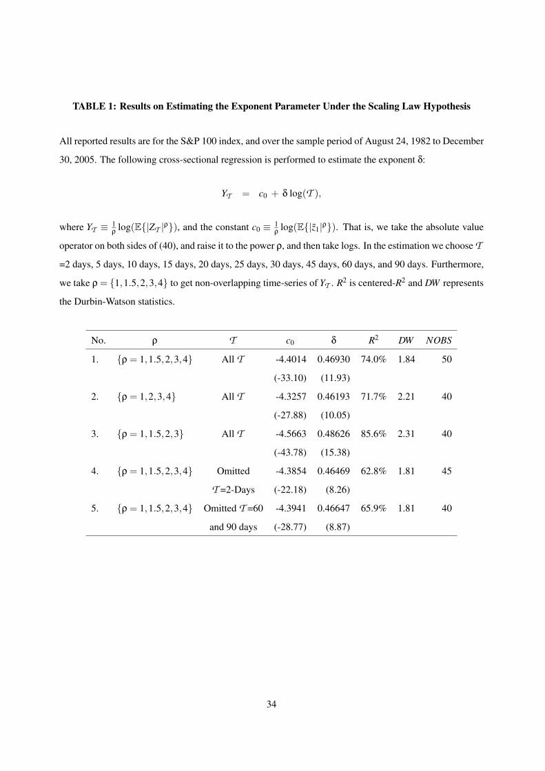
TABLE 1: Results on Estimating the Exponent Parameter Under the Scaling Law Hypothesis

All reported results are for the S&P 100 index, and over the sample period of August 24, 1982 to December

30, 2005. The following cross-sectional regression is performed to estimate the exponent δ:

YT = c0 + δ log(T ),

where YT ≡ 1ρ log(E{|ZT |ρ}), and the constant c0 ≡ 1

ρ log(E{|z1|ρ}). That is, we take the absolute value

operator on both sides of (40), and raise it to the power ρ, and then take logs. In the estimation we choose T

=2 days, 5 days, 10 days, 15 days, 20 days, 25 days, 30 days, 45 days, 60 days, and 90 days. Furthermore,

we take ρ = {1,1.5,2,3,4} to get non-overlapping time-series of YT . R2 is centered-R2 and DW represents

the Durbin-Watson statistics.

No. ρ T c0 δ R2 DW NOBS

1. {ρ = 1,1.5,2,3,4} All T -4.4014 0.46930 74.0% 1.84 50

(-33.10) (11.93)

2. {ρ = 1,2,3,4} All T -4.3257 0.46193 71.7% 2.21 40

(-27.88) (10.05)

3. {ρ = 1,1.5,2,3} All T -4.5663 0.48626 85.6% 2.31 40

(-43.78) (15.38)

4. {ρ = 1,1.5,2,3,4} Omitted -4.3854 0.46469 62.8% 1.81 45

T =2-Days (-22.18) (8.26)

5. {ρ = 1,1.5,2,3,4} Omitted T =60 -4.3941 0.46647 65.9% 1.81 40

and 90 days (-28.77) (8.87)

34

TABLE 2: Distributional Features of the S&P 100 Index

The sample period for S&P 100 index options is January 1984 to December 2005. Our tests are based

on out-of-money calls and puts with maturity fixed at either 28-days or 56-days. For the contract cycle

of 28 days, there are an average of 8 calls and 12 puts with a total of 5373 calls and puts. With 56 days

maturity, there are an average of 7 calls and 9 puts with a total of 2135 options. Each pricing distribution is

constructed based on the theoretical relations in (52)-(55). Features of the daily physical return distribution

reported in Panel B are based on the time-series of daily realized returns, z, and its powers.

Panel A: Pricing Distributions

28-Day Maturity 56-Day Maturity

Series Mean Std Mean Std

µq1(t,T ) 2.5747e-003 2.6715e-003 5.1051e-003 5.1409e-003

µq2(t,T ) 2.7775e-003 3.8055e-003 5.5312e-003 7.0080e-003

µq3(t,T ) -2.7063e-004 8.3506e-004 -5.5063e-004 1.4915e-003

µq4(t,T ) 9.6243e-005 3.7167e-004 2.2890e-004 7.7483e-004

Varianceq(t,T ) 2.7638e-003 3.7861e-003 5.4789e-003 6.9653e-003

Skewnessq(t,T ) -1.5681e+000 1.3038e+000 -1.0130e+000 7.1998e-001

Kurtosisq(t,T ) 1.0933e+001 1.5907e+001 5.5390e+000 2.4946e+000

Panel B: Daily Physical Return Distributions (08:24:1982:12:30:2005, NOBS=5912)

Series Mean Std Skewness Kurtosis

z 3.9574e-004 1.1231e-002 -1.685 41.3

z2 1.2627e-004 7.9873e-004 60.307 4219.1

z3 -2.2368e-006 1.7597e-004 -75.496 5768.8

z4 6.5380e-007 4.1618e-005 76.737 5896.0

35

TABLE 3: Estimates of the Risk Aversion Distribution

Results reported below for the distribution of risk aversion are based on the term distribution of risk-neutral

density and physical density. According to Theorem 1, the raw moments of the risk aversion distribution

are given by,

A1 ≈ µq3(t,T )

µq4(t,T )

− µp3(t,T )

µp4(t,T )

,

A2 ≈ 2(

µq2(t,T )

µq4(t,T )

− µp2(t,T )

µp4(t,T )

− µp3(t,T )×A1

µp4(t,T )

),

A3 ≈ 6(

µq1(t,T )

µq4(t,T )

− µp1(t,T )

µp4(t,T )

− µp2(t,T )×A1

µp4(t,T )

− µp3(t,T )×A2

2µp4(t,T )

),

A4 ≈ 24(

1µq

4(t,T )− 1

µp4(t,T )

− µp1(t,T )×A1

µp4(t,T )

− µp2(t,T )×A2

2µp4(t,T )

− µp3(t,T )×A3

6µp4(t,T )

),

where µp1 (t,T )

µp4 (t,T ) , µp

2 (t,T )µp

4 (t,T ) , and µp3 (t,T )

µp4 (t,T ) are 28-days, or 56-days, moments extracted from daily returns under

the hypothesis of scaling laws in (40). This calculation uses an exponent value δ = 0.46930 (from Table

1). The risk-neutral moments for 28-days and 56-days distributions are calculated from observed option

prices on the S&P 100 index. The standard deviation of the risk aversion distribution, Std[φ], is computed

as√A2−A2

1, Skewness[φ]= (A3 − 3A2A1 + 2A31)/(Std[φ])3, and Kurtosis[φ] = (A4 − 3A4

1 + 6A2A21 −

4A3A1)/(Std[φ])4. The negative value of Mean[φ] indicates positive risk aversion.

Mean[φ] Std[φ] Skewness[φ] Kurtosis[φ]

Panel A. Distribution of Risk Aversion, 28-Days -2.0957 5.7791 2.7667 161.19

Panel B. Distribution of Risk Aversion, 56-Days -1.8882 5.8290 2.1648 91.75

36

−2.8 −2.6 −2.4 −2.2 −2 −1.8 −1.6 −1.4 −1.2

0.05

0.1

0.15

0.2

0.25

0.3

Risk Aversion

Freq

uenc

y

Implied Density of Risk Aversion

Fig. 1. Density Function of the Risk Aversion DistributionThis graph plots the density function corresponding to the moments of the risk aversion distribution re-ported in Panel A of Table 3. The construction of the density is based on the assumption that risk aversionfollows the variance-gamma random variable (Madan, Carr, and Chang (1998)). This variable has a closed-form density in terms of the modified Bessel function of the second kind. For the variance gamma randomvariable, Xvg[µ,ζv,ζs,ζk], there is a unique transformation between the parameters ζv, ζs, ζk and volatility,skewness, and kurtosis of the distribution. When Xvg[ζv,ζs,ζk] is calibrated to ζv = 5.76, ζs = 48.16, andζk = 0.09 respectively, it mimics the desired risk aversion moments for 28 day term. The negative valueson the x-axis indicate that the mean risk aversion is positive.

37