the distribution of income in industrialized countries · the evidence presented is a...

The Distribution of Incomein Industrialized Countries

A.B. Atkinson

Introduction and summary

This paper is about recent developments in the distribution ofincome in industrialized, and particularly, the G-7 countries. Limit-ing the geographical focus in this way ignores the important changestaking place in transition economies and in the developing world, butI have chosen to focus on the countries I know best, which is why asmall, offshore European island receives disproportionate attention.

The paper makes four main points.

(1) There is considerable diversity of national experience withregard to the distributions of income and earnings; it ismisleading to talk of a general “trend” toward increaseddispersion.

(2) Differences in income distribution can have a sizable impacton the assessment of living standards across countries, andon the measured rate of growth of living standards.

(3) The evolution of income distribution cannot be explainedsolely in terms of earnings; there has been a significantturnaround in capital incomes; there have been changes inthe extent of fiscal redistribution.

11

(4) The links between macroeconomic variables and the distri-bution of personal income are complex; this is an impor-tant area for further study.

Qualifications

Any account of the empirical evidence must be prefaced withwarnings about the shortcomings of the underlying data and aboutthe many conceptual issues, which need to be addressed. Theseissues are discussed at length in a study for the Organization for Eco-nomic Cooperation and Development (OECD) by Atkinson, Rain-water, and Smeeding (1995). I should emphasize in particular thatthe evidence presented is a “snapshot” of the income distribution.Creating individual life histories at a national level is a challengingtask on the research agenda, and I have seen no satisfactory cross-country studies.

Diversity of national experience

The United States, the United Kingdom, and a number of otherOECD countries, have experienced rising income dispersion sincethe 1970s. Chart 1, based on national studies of the distribution ofequivalent disposable household income, shows that this has beenespecially marked in the United Kingdom, where the Gini coeffi-cient (a summary measure of income differences) rose by nearlyhalf—a very large increase by historical standards. The rise in theUnited Kingdom seems to have been particularly sharp in the secondhalf of the 1980s, coming to an end after 1990, when the Gini coeffi-cient appears to have levelled off or turned down.

In the United States, Japan, and West Germany, increases in dis-persion are more modest. Between 1979 and the 1990s, the Ginicoefficient in the United States rose from 40 percent to 44 percent(that is, from an index of 100 to 110). But an increase of one-tenth isstill significant for a statistic of which Henry Aaron once remarkedthat “following these data was like watching the grass grow” (1978,p. 17). That may have been true in the 1970s (see Chart 1), but ceasedto be true in the 1980s.

12 A.B. Atkinson

Yet dispersion increased neither at the same rate nor universally.Over the period shown, there was no increase in Canada, France, nor(over the period as a whole) in Italy. There are contrasting nationalexperiences, even within the G-7. The same applies if attention isfocused on the bottom of the distribution. Taking the European Com-mission definition of financial poverty as living below half thenational average, we find that the United Kingdom stands out for itssharp rise in poverty over the 1980s, whereas other countries haveseen either a more modest increase or no overall trend. See Chart 2.The rate for the United States (which is not the official poverty rate,

The Distribution of Income in Industrialized Countries 13

Chart 1Changes in Income Dispersion

Relative to 1977

Sources: Canada, Gottschalk and Smeeding, 1997, Appendix Table B; France (1975 = 100),Atkinson, 1997, Table FR2, Synthèses series; (West) Germany (1978 = 100), Becker, 1996,Table 1, and Hauser, 1996, Table 1, linked at 1993 using Becker, 1998, Table 4; Italy, Atkin-son, 1997, Table IT2, Bank of Italy series; Japan (1981 = 100), Gottschalk and Smeeding,1997, Appendix Table B; United Kingdom, Atkinson, 1997, Table UK3, series constructedby Goodman and Webb; United States, U.S. Department of Commerce, 1993, Table B-3, p.B-6.

80

90

100

110

120

130

140

150

1975 1979 1983 1985 1989 19951977 19871981 1991 1993

Canada

Gini coefficient (1977=100)

80

90

100

110

120

130

140

150

Gini coefficient (1977=100)

UK

Japan

WestGermany

US

Italy

France

but the percentage below half the median) went up by a few percent-age points between the mid-1970s and the mid-1990s.

The picture of diversity applies when we look at the distribution ofindividual earnings in Chart 3, which shows the changes since 1977in the decile ratio. The decile ratio is the ratio of earnings at the topdecile (the person 10 percent from the top) to those at the bottomdecile (the person 10 percent from the bottom). The United Kingdomagain shows the largest change: a rise of one-fifth in the decile ratio.But it stands out less sharply. As is well known, the ratio increased inthe United States. For the other countries, the pattern is more mixed,with a rise and then a fall in Canada, and a fall and then a rise in Italy.

14 A.B. Atkinson

Chart 2Changes in Low Income Since 1977

Sources: Canada, Statistics Canada, 1996, pp. 25-6; France (1975 = 100), Atkinson, 1997,Table FR3, Synthèses series; Italy, Atkinson, 1997, Table IT4, Commissione series; UnitedKingdom, Atkinson, 1997, Table UK4, series constructed by Goodman and Webb, andHouseholds Below Average Income series; United States, Smeeding, 1997, Table A-4, per-centage below 50 percent of median.

Italy

50

100

150

200

250

300

350

50

100

150

200

250

300

350

Index of low income 1977=100(1979 for US, 1980 for Canadaand Italy, 1984 for France)

Index of low income 1977=100(1979 for US, 1980 for Canada

and Italy, 1984 for France)

UK

Canada

US

France

1977 1983 1985 1989 19951979 19871981 1991 1993

Nor are there signs that the United States and the United Kingdomwere leading indicators, with Europe catching up behind. As theOECD has observed,

“No clear tendency emerges of a generalized increase in earningsinequality over the first half of the 1990s. Of the 16 countries ... dis-persion increased in half of them, and was either broadly unchangedor declined somewhat in the rest” (1996, p. 63).

It is misleading, therefore, to talk of a general “trend” toward


Chart 3Changes in Earnings Dispersion Relative to 1977

Sources: France, Bayet and Julhès, 1996, p. 48; Canada (1981 = 100), OECD, 1996, Table3.1; (West) Germany (1983 = 100), OECD, 1996, Table 3.1; Italy, Brandolini and Sestito,1996, Table 8; Japan (1981 = 100), OECD, 1996, Table 3.1; United Kingdom, Atkinson andMicklewright, 1992, Table BE1, linked at 1990 to Department of Employment, 1997, TableA30.2; United States, Karoly, 1994, Table 2B.2, weekly (consistent) wage and salaryincome, linked at 1979 and 1987, linked in 1989 to OECD, 1996, Table 3.1, which refers tomale earnings.

Italy

.7

.8

.9

1

1.1

1.2

1.3

.7

.8

.9

1

1.1

1.2

1.3

1977=1 (1979 for Japan,1981 for Canada and1983 for West Germany)

1977=1 (1979 for Japan,1981 for Canada and

1983 for West Germany)

UK

Canada

US

WestGermany

1967 ‘73 ‘75 ‘79 ‘85‘69 ‘77‘71 ‘81 ‘83 ‘87 ‘89 ‘91 ‘93 ‘95 ‘97

Japan

France

US

France

UK

increased dispersion, and even in countries where dispersion hasincreased, the historical record is better described as consisting of“episodes” of widening income differences rather than as followingan inexorable trend.

Distributional differences matter

A recent study by three World Bank economists concluded thatincome dispersion varies significantly across countries, but thatwithin most countries, there is little significant variation over time(Li, Squire, and Zou, 1998). I agree with the first conclusion but notwith the second.

Chart 4 shows the Gini coefficients for disposable householdincomes in different OECD countries relating mostly to the early1990s (although 1984 for France and West Germany). There is aclear geographic pattern, with Scandinavia and Benelux having thelowest coefficients, followed by the large mainland European coun-tries, southern Europe, and then the Anglo-Saxon countries. Therange is from 23 percent in Finland to 35 percent in the United States.As has been pointed out by Richard Freeman, the differencesbetween the United States and Europe in the distribution ofearningsmean that the low paid in the United States fall far behind many oftheir European counterparts. According to his estimates, the hourlycompensation in purchasing power of the American man at the bot-tom decile is half that of the comparable Italian (1994, p. 13). Howfar is the same true of household disposable incomes? National Dis-posable Income per head adjusted using purchasing power paritieswas 39 percent higher in the United States in 1990 than in the Euro-pean Community (the then 12 members). The share of the bottomfifth in the United States was 5.7 percent. This means that, evenallowing for a difference in real mean income of 39 percent, the bot-tom fifth in the United States would be worse off than an “averageEuropean” living in a country where the share of the bottom fifth wasgreater than 8 percent. If we take the concrete case of Germany,where the share of the bottom fifth was 9.8 percent, and real incomeonly 18 percent lower than in the United States, then this group as awhole is 40 percent better off than their counterparts in the United

16 A.B. Atkinson

States. Such a calculation is, of course, open to objections. There aredifferences across countries between National Disposable Incomeper head and mean household equivalent income. The purchasingpower adjustment can be debated. But the difference is so large that itis unlikely to be affected by the choice of a different basis for conver-sion. The differences in income distribution have a sizable impact onthe assessment of living standards across countries.


Chart 4Gini Coefficients in OECD Countries

Early 1990s

Sources: Gottschalk and Smeeding, forthcoming, Chart 2. Figures relate to 1987 (Ireland),1989 (France), 1990 (Spain), 1991 (Finland, Netherlands, Italy), 1992 (Belgium, Denmark,Sweden), 1994 (Germany, Luxembourg, United States), 1995 (Norway, United Kingdom).The estimates relate to household disposable income per equivalent adult using an equiva-lence scale of the square root of household size and using individual weights.

Fin

lan

d

No

rwa

y

Lu

xem

bo

urg

We

stG

erm

an

y

Ca

na

da

Sw

ed

en

De

nm

ark

Be

lgiu

m

Ita

ly

Ne

the

rla

nd

s

Fra

nce

Sp

ain

Au

stra

lia

Cze

chR

ep

ub

lic

Un

ited

Kin

gd

om

Un

ited

Sta

tes0

5

10

15

20

25

35

40

0

5

10

15

20

25

35

40

Gini coefficientpercent


Ire

lan

d

3030

As we have seen in Chart 1, some G-7 countries have seen a sub-stantial rise in income dispersion over the 1980s. This can make asignificant difference to the measured growth performance. Supposethat national income were to be distributionally adjusted by multi-plying by (1-Gini coefficient), as proposed by Sen (1976), then wewould get a different perspective of growth rates. For example, tak-ing the periods 1973-1979 and 1979-1989 (as used by the OECD initsHistorical Statistics), the United Kingdom performance was con-siderably better in the 1980s than the 1970s on an unadjusted basis,but this improvement disappears when the distributional adjustmentis made. The measured growth rate is effectively halved. Put differ-ently, those at the bottom did not share in rising prosperity.

This evidence suggests that the distribution of income can changewithin countries in a way that is economically significant.

Behind the income dispersion

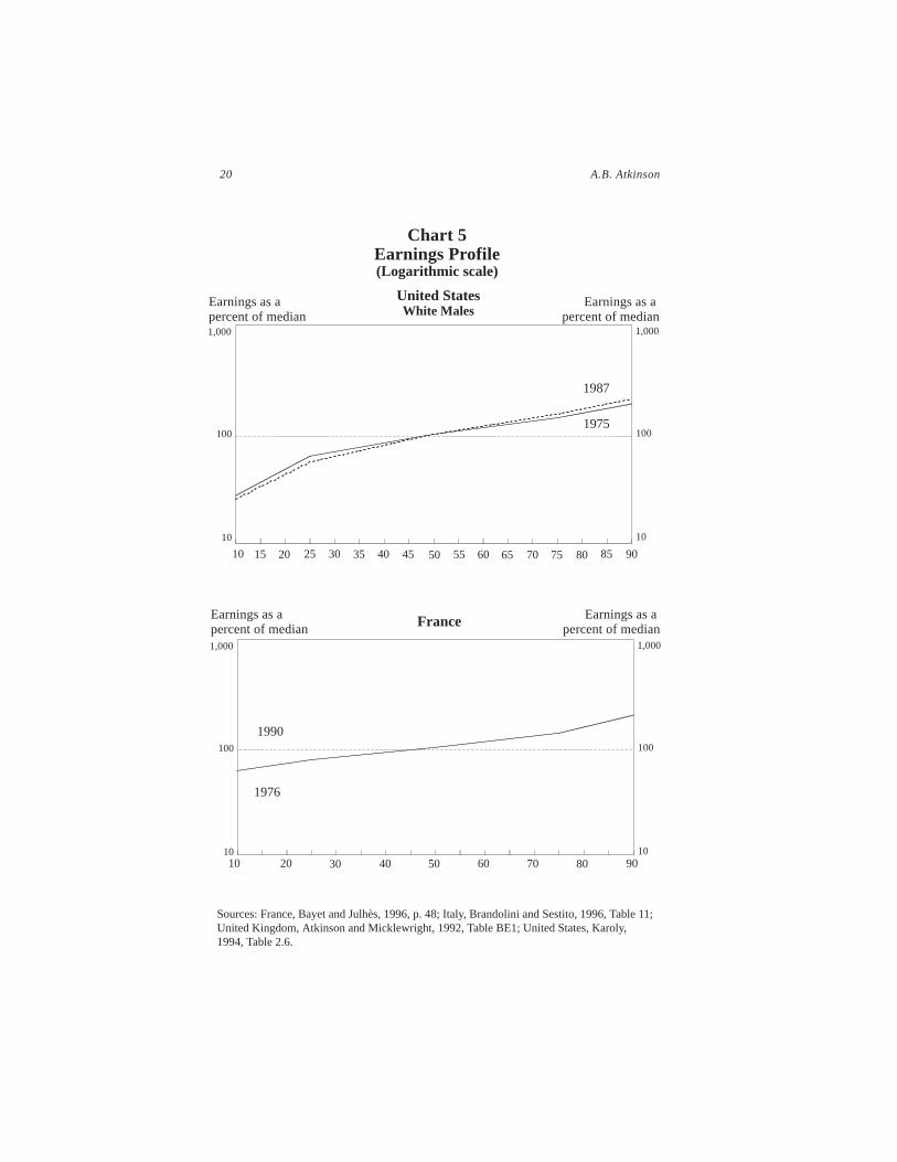
So far I have simply looked at a single summary statistic of disper-sion, whereas in order to understand the changes, we need to look atthe distribution as a whole. Chart 5 shows the profile of earnings infour of the G-7 countries and how it has changed since the late 1970s.The charts are similar to the famous “parade” of incomes describedby the Dutch economist, Jan Pen, in which he envisaged everyonemarching past in an hour, with their height corresponding to theirearnings. After six minutes, we come to the tenth percentile, the firstpoint in Chart 5, where people are about three feet tall; in the 54thminute, we enter the top 10 percent, where people are only about 12feet tall; but then heights shoot up, reaching 500 feet or more. (Theseare not shown.)

In a paper to this symposium four years ago, Paul Krugman (1994)drew a diagram in which the earnings profile rotated, arguing thatthis explains both the widening wage dispersion in the United Statesand the increased unemployment in Europe. The latter arose becausethe European welfare state, and minimum wage provisions, put afloor on wages. However, if rotation of the wage/skill nexus were thefull explanation, then we would expect to find the rise at the top in

18 A.B. Atkinson

Europe, even if there were no change at the bottom. From Chart 5, itcan be seen that there is little evidence of this happening. Even onthis microscopic (logarithmic) scale, the United States and theUnited Kingdom stand out for the extent of the change at the top aswell as at the bottom.

A further important feature of the changes in the earnings distribu-tion is what Krugman has called its “fractal” quality: One continuesto find an increase in dispersion even if one considers narrowlydefined groups. Katz and Murphy have documented in the UnitedStates the “striking increase in wage inequality within groups” clas-sified by sex, education, and work experience (1992). In the UnitedKingdom, there has been increased dispersion even within narrowlydefined occupation groups (Atkinson, 1997a).

It is possible to attribute all of this to unobserved differences inskill, but other explanations seem worth exploring. There are reasonsto suppose that there has been a shift from company pay policies toindividual negotiation, and for conventional pay norms to breakdown. This process may acquire a dynamic of its own: As more peo-ple are remunerated outside the conventional norms, so adherence tothese norms becomes weaker, and the socially acceptable range ofremuneration widens.

Alan Blinder once said, “If you want to understand the rise inincomeinequality in the 1980s, the place to start is with the rise inwageinequality” (1993, p. 308).

I agree, but one should not stop there. One has to remember thatthere are several steps in going from individual earnings to house-hold incomes. (See the Box 1.) Where more than one person isemployed, we have to add together their earnings. We have to considerwealth, which generates capital income in the form of rent, divi-dends, and interest, or indirectly in the form of pensions, paymentsfrom life assurance, and so forth. Real rates of interest have risen,and this is one potential cause of widening dispersion, which hastended to be overlooked. In a simple human capital model, highercosts of borrowing lead to wider compensating differentials.


20 A.B. Atkinson

Chart 5Earnings Profile(Logarithmic scale)

Sources: France, Bayet and Julhès, 1996, p. 48; Italy, Brandolini and Sestito, 1996, Table 11;United Kingdom, Atkinson and Micklewright, 1992, Table BE1; United States, Karoly,1994, Table 2.6.

1987

1975

Earnings as apercent of median


United StatesWhite Males

Earnings as apercent of medianFranceEarnings as a

percent of median

10 25 30 40 5515 3520 45 50 60 65 70 75 80 85

10 30 4020 50 60 70 80 90

100

1,000

100

1,000

1010

10

100

1,000

10

1,000

100

1990

1976

90


Chart 5 - continuedEarnings Profile(Logarithmic scale)

Sources: France, Bayet and Julhès, 1996, p. 48; Italy, Brandolini and Sestito, 1996, Table 11;United Kingdom, Atkinson and Micklewright, 1992, Table BE1; United States, Karoly,1994, Table 2.6.

1990

1977


Earnings as apercent of medianUnited Kingdom


ItalyEarnings as apercent of median

10 25 30 40 5515 3520 45 50 60 65 70 75 80 85

10 30 4020 50 60 70 80 9010

100

1,000

10

100

1,000

10

100

1,000

10

100

1,000

1989-93

1977-79

90

As well as capital incomeand private transfers, wehave to add transfers paidby the state, and deduct theamounts paid in income taxand social insurance contri-butions, in order to arrive atdisposable income. Thereis, therefore, no reason toexpect dispersion of dispos-able household income tofollow slavishly dispersionin individual pre-tax earn-ings. As Chart 6 shows forthe United Kingdom, in thatcountry the two seriesmoved closely togetherfrom 1975 to 1984, but thenincome dispersion rosemore rapidly.

One proximate reason for the divergence in the United Kingdom isthe shift in redistributive fiscal policy after the mid-1980s. This isillustrated in Chart 7, which shows the dispersion of market income(“Pre”) and income after tax and benefits (“Post”). The Gini coeffi-cient for market income has varied cyclically, but the predominantimpression is of a long-run rise since the mid-1960s. In the 20 yearsfrom 1965 to 1984, the coefficient increased from 40 percent to 50percent. What is even more striking is that the coefficient for post-government income showed scarcely any rise over this period. Theredistributive impact of cash transfers and taxation increased byenough to offset the more unequal market incomes. After 1984, thestory is quite different. The line for market income continued to rise,but between 1984 (marked by an arrow) and 1990, the Gini coeffi-cient for post-government income increased much more sharply.Measured in terms of the difference between the two coefficients, theredistributive contribution of transfers and taxes fell from 19 per-centage points (the difference between the two Gini coefficients in

22 A.B. Atkinson

Box 1From Individual

Earnings to HouseholdDisposable Income

Earnings of Person 1+

Earnings of Person 2+

Income from capital+

Private transfers+

State transfers–

Direct taxes=

Disposable income/

Number of equivalent adults=

Equivalent Disposable Income

1984) to 11 percentage points. The interpretation of these calcula-tions raises a number of major issues, such as the incidence of taxa-tion, the separation of life cycle from other redistribution, and thevaluation of public spending on goods and services. But, taken atface value, they suggest that the state budget has ceased to offset therising dispersion of market incomes, and that the steeper rise in theGini coefficient from 1984 to 1990 was associated with reducedredistributive ambitions of the government.

Links between macro variables and the personaldistribution of income

What is the relationship between the distributional evidence sum-marized above and the macroeconomy? On the one hand, there are


Chart 6Dispersion of Individual Earnings and Disposable

Household Income in UK

Sources: Income from Goodman and Webb, 1994, p. A2; earnings from Atkinson and Mick-lewright, 1992, Table BE1, extended using data fromNew Earnings Survey(for example,Department of Employment, 1997).

Gini coefficient percent Gini coefficient percent

Earnings

20

24

26

28

30

32

34

20

24

26

28

30

32

34

Income

1968 ‘94‘70

2222

‘72 ‘76‘74 ‘78 ‘80 ‘84‘82 ‘86 ‘88 ‘90 ‘92

expectations that an economic downturn slowed the growth of highincomes in the United States:

"The slowing growth of household income inequality wasno doubt related to the winding down of the economic ex-pansion of the 1980s and the ensuing recession in the early1990s" (Ryscavage, 1995, p. 54).

On the other hand, at least up to the 1980s, a 1 percent rise in theU.S. unemployment rate was associated with a 1 percent increase inthe official poverty rate (Blinder and Blank, 1986).

24 A.B. Atkinson

Chart 7Income Before and After Government Budget in UK

Sources: First series (from 1961) distribution (not equivalized) among households of originalincome and final income: 1961-1975, from Royal Commission on the Distribution of Incomeand Wealth, 1977, pp. 247 and 251; 1976, from Central Statistical Office,Economic Trends,January 1982, p. 105 (for 1976) and December 1982, p. 112 (for 1978).

Second series (from 1977) distribution among households of equivalized original incomeand post-tax income:Economic Trends, April 1998, p. 58 (for 1977, 1979, 1981, 1983, 1985,1987, 1989, 1991, 1993-94 to 1996-97), December 1994, p. 65 (for 1978, 1980, 1982, 1984,1986, 1988, 1992), and January 1993, p. 159 (for 1990).

0

10

20

30

40

60

0

10

20

30

40

60



5050

1961 ‘67 ‘69 ‘73 ‘79‘63 ‘71‘65 ‘75 ‘77 ‘81 ‘83 ‘85 ‘87 ‘89 ‘95‘91 ‘93

POST

PRE

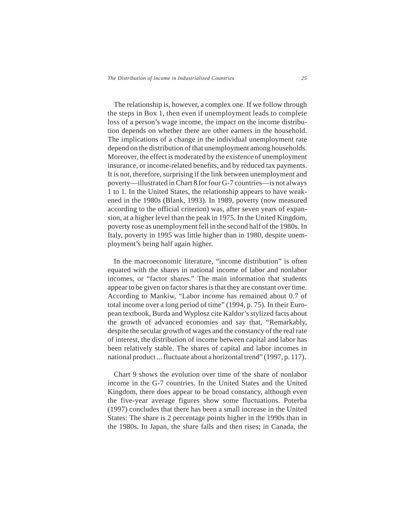
The relationship is, however, a complex one. If we follow throughthe steps in Box 1, then even if unemployment leads to completeloss of aperson’s wage income, the impact on the income distribu-tion depends on whether there are other earners in the household.The implications of a change in the individual unemployment ratedepend on the distribution of that unemployment among households.Moreover, the effect is moderated by the existence of unemploymentinsurance, or income-related benefits, and by reduced tax payments.It is not, therefore, surprising if the link between unemployment andpoverty—illustrated in Chart 8 for four G-7 countries—is not always1 to 1. In the United States, the relationship appears to have weak-ened in the 1980s (Blank, 1993). In 1989, poverty (now measuredaccording to the official criterion) was, after seven years of expan-sion, at a higher level than the peak in 1975. In the United Kingdom,poverty rose as unemployment fell in the second half of the 1980s. InItaly, poverty in 1995 was little higher than in 1980, despite unem-ployment’s being half again higher.

In the macroeconomic literature, “income distribution” is oftenequated with the shares in national income of labor and nonlaborincomes, or “factor shares.” The main information that studentsappear to be given on factor shares is that they are constant over time.According to Mankiw, “Labor income has remained about 0.7 oftotal income over a long period of time” (1994, p. 75). In their Euro-pean textbook, Burda and Wyplosz cite Kaldor’s stylized facts aboutthe growth of advanced economies and say that, “Remarkably,despite the secular growth of wages and the constancy of the real rateof interest, the distribution of income between capital and labor hasbeen relatively stable. The shares of capital and labor incomes innational product ... fluctuate about a horizontal trend” (1997, p. 117).

Chart 9 shows the evolution over time of the share of nonlaborincome in the G-7 countries. In the United States and the UnitedKingdom, there does appear to be broad constancy, although eventhe five-year average figures show some fluctuations. Poterba(1997) concludes that there has been a small increase in the UnitedStates: The share is 2 percentage points higher in the 1990s than inthe 1980s. In Japan, the share falls and then rises; in Canada, the


26 A.B. Atkinson

Chart 8Percent in Poverty and Unemployment

Sources: See Chart 2 for poverty figures; unemployment figures from OECD, 1997 (disketteversion), Table 2.15.

Poverty

Unemployment

United States

United Kingdom

0

2

4

6

8

10

14

16

12

0

2

4

6

8

10

14

16

12

5

10

15

20

25

0

1972 ‘76 ‘80 ‘82 ‘86 ‘94‘74 ‘84‘78 ‘90 ‘92‘88

‘88 ‘92‘90‘78 ‘84‘74 ‘94‘86‘82‘80‘761972

Poverty

Unemployment

0

25

20

15

10

5


Chart 8 - continuedPercent in Poverty and Unemployment

Sources: See Chart 2 for poverty figures; unemployment figures from OECD, 1997 (disketteversion), Table 2.15.

Poverty

Unemployment

Canada

Italy

0

5

10

20

15

0

5

10

20

15

5

10

15

20

0

1972 ‘76 ‘80 ‘82 ‘86 ‘94‘74 ‘84‘78 ‘90 ‘92‘88

1987 199319901978 19841975 19811972

Poverty

Unemployment

0

20

15

10

5

28 A.B. Atkinson

Source: Poterba, 1997, Table 8 (five-year moving averages of shares).

Chart 9Non-Labor Share

Canada

UK

Anglo-Saxon Countries and Japan

1966 ’70 ‘76 ‘78 ‘84 ‘94‘68 ‘82‘72 ‘88 ‘92‘86‘74 ‘80 ‘90

Percent value addedPercent value added

US

Japan

Percent value addedEurope

Percent value added

199019871972 19811969 19931984197819751966

Italy

France

WestGermany

29

41

45

43

39

37

35

33

27

25

29

41

45

43

39

37

35

33

27

25

3131

31

25

27

33

35

37

39

43

45

41

29

31

25

27

33

35

37

39

43

45

41

29

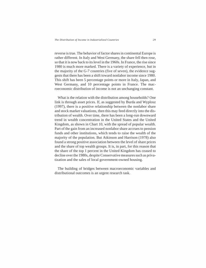
reverse is true. The behavior of factor shares in continental Europe israther different. In Italy and West Germany, the share fell then rose,so that it is now back to its level in the 1960s. In France, the rise since1980 is much more marked. There is a variety of experience, but inthe majority of the G-7 countries (five of seven), the evidence sug-gests that there has been a shift toward nonlabor income since 1980.This shift has been 5 percentage points or more in Italy, Japan, andWest Germany, and 10 percentage points in France. The mac-roeconomic distribution of income is not an unchanging constant.

What is the relation with the distribution among households? Onelink is through asset prices. If, as suggested by Burda and Wyplosz(1997), there is a positive relationship between the nonlabor shareand stock market valuations, then this may feed directly into the dis-tribution of wealth. Over time, there has been a long-run downwardtrend in wealth concentration in the United States and the UnitedKingdom, as shown in Chart 10, with the spread of popular wealth.Part of the gain from an increased nonlabor share accrues to pensionfunds and other institutions, which tends to raise the wealth of themajority of the population. But Atkinson and Harrison (1978) alsofound a strong positive association between the level of share pricesand the share of top wealth groups. It is, in part, for this reason thatthe share of the top 1 percent in the United Kingdom has ceased todecline over the 1980s, despite Conservative measures such as priva-tization and the sales of local government-owned housing.

The building of bridges between macroeconomic variables anddistributional outcomes is an urgent research task.


References

Aaron, H.J.Politics and the Professors.Washington, D.C.: Brookings Institution, 1978.Atkinson, Anthony B. “Measurement of Trends in Poverty and the Income Distribution,”

Microsimulation Unit Working Paper MU9701, Department of Applied Economics, Cam-bridge,1997.

Atkinson, A.B. “Bringing Income Distribution in from the Cold,”Economic Journal, vol. 107,pp. 297-321,1997a.

__________, J.P.F. Gordon, and A.J. Harrison. “Trends in the Shares of Top Wealth-Holders inBritain, 1923-1981,”Oxford Bulletin of Economics and Statistics, vol. 51, 1989, pp.315-31.

__________, and A.J. Harrison.Distribution of Personal Wealth in Britain. Cambridge: Cam-bridge University Press, 1978.

30 A.B. Atkinson

Chart 10Share of Top 1 Percent in Total Personal Wealth

in United States and United Kingdom

Sources: UK: 1923-1972 from Atkinson and Harrison, 1978, Table 6.5. (Note that there arebreaks in the series between 1938 and 1950 and 1959 and 1960, and that the estimates before1950 relate to England and Wales; those after relate to Great Britain. These estimates arecontinued to 1982 from Atkinson, Gordon, and Harrison, 1989, Table 1. The estimates from1976 are produced on a different basis by the Inland Revenue, and relate to the United King-dom. Sources:Inland Revenue Statistics, 1972, Table 11.5 and 1997, Table 13.5. US: 1922-1981 from Wolff, 1992, Table 1; 1962-1989 from Wolff, 1994, Table 4.

UnitedStates II

United Kingdom

0

20

30

40

50

60

70

0

20

30

40

50

60

70

1922 1946 1952 1964 19881928 19581934 197619701940 1982

Share in totalpersonal wealth

Share in totalpersonal wealth

Great Britain

Englandand Wales

10 10

United States I

1994

__________, and J. Micklewright.Economic Transformation in Eastern Europe and the Dis-tribution of Income. Cambridge: Cambridge University Press, 1992.

__________, L. Rainwater, and T. Smeeding.Income Distribution in OECD Countries.Paris:OECD, 1995.

Bayet, Alain, and Martine Julhès.Séries Longues sur les Salaires, Emploi-Revenus no.105.Paris: INSEE, 1996.

Becker, Irene. “Die Entwicklung der Einkommensverteilung und der Einkommensarmut inden alten Bundesländern von 1962 bis 1988” in Irene Becker and Richard Hauser, “Ein-kommensverteilung und Armut in Deutschland von 1962 bis 1995,” Arbeitspapier Nr. 9,EVS-Projekt, Universität Frankfurt am Main, 1996.

__________. “Zur personellen Einkommensverteilung in Deutschland,”Arbeitspapier Nr. 13,EVS-Projekt, Universität Frankfurt am Main, 1998.

Blank, R. M. “Why Were Poverty Rates so High in the 1980s?” in D.B. Papadimitriou and E.N.Wolff, eds.,Poverty and Prosperity in the USA in the Late Twentieth Century. Basingstoke:Macmillan, 1993.

__________, and A.S. Blinder. “Macroeconomics, Income Distribution, and Poverty,” in S.H.Danziger and D.H. Weinberg, eds.,Fighting Poverty.Cambridge, Massachusetts: HarvardUniversity Press, 1986.

Blinder, A.S. “Comment” in D.B. Papadimitriou and E.N. Wolff, eds.,Poverty and Prosperityin the USA in the Late Twentieth Century.Basingstoke: Macmillan, 1993.

Brandolini, Andrea, and Paolo Sestito. “Earnings Dispersion in Italy, 1977-1995,” Bank ofItaly, 1996.

Burda, M., and C. Wyplosz.Macroeconomics, 2nded. Oxford: Oxford University Press, 1997.Central Statistical Office.Economic Trends.London: HMSO, various years.Department of Employment.New Earnings Survey.London: HMSO, 1979.__________.New Earnings Survey.London: HMSO, 1990.__________. New Earnings Survey.London: HMSO, 1997.Freeman, R. B. “How Labor Fares in Advanced Economies” in R.B. Freeman, ed.,Working

Under Different Rules. New York: Russell Sage Foundation, 1994.Goodman, A., and S. Webb.For Richer, For Poorer, IFS Commentary no. 42. London: IFS,

1994.Gottschalk, Peter, and Timothy M. Smeeding. “Cross-National Comparisons of Earnings and

Income Inequality,”Journal of Economic Literature, vol. 35 (June 1997), pp. 633-87.__________, and ___________. “Empirical Evidence on Income Inequality in Industrialized

Countries” in A.B. Atkinson and F. Bourguignon, eds.,Handbook of Income Distribution.Amsterdam: North Holland, forthcoming.

Hauser, Richard. “Vergleichende Analyse der Einkommensverteilung und der Einkommen-sarmut in den alten und neuen Bundesländern von 1990 bis 1995” in Irene Becker and Rich-ard Hauser, “Einkommensverteilung und Armut in Deutschland von 1962 bis 1995,”Arbeitspapier Nr. 9, EVS-Projekt, Universität Frankfurt am Main, 1996.

Karoly, Lynn A. “The Trend in Inequality Among Families, Individuals, and Workers in theUnited States: A Twenty-Five-Year Perspective” in Sheldon Danziger and Peter Gott-schalk, eds.,Uneven Tides.New York: Russell Sage Foundation, 1994.

Katz, L., and K. Murphy. “Changes in Relative Wages, 1963-1987: Supply and Demand Fac-tors,” Quarterly Journal of Economics, vol. 107, 1992, pp. 35-78.

Krugman, Paul. “Past and Prospective Causes of High Unemployment” inReducing Unem-ployment: Current Issues and Policy Options.Papers and proceedings from a symposiumsponsored by the Federal Reserve Bank of Kansas City in Jackson Hole, Wyoming, August25-27, 1994.

Li, H., L. Squire, and H. Zou. “Explaining International and Intertemporal Variations inIncome Inequality,”Economic Journal, vol. 108, 1998, pp. 26-43.

Mankiw, N. G.Macroeconomics.New York: Worth, 1994.


OECD.Employment Outlook.Paris: OECD, 1996.__________.Historical Statistics.Paris: OECD, 1997.Poterba, J.M. “The Rate of Return to Corporate Capital and Factor Shares,”NBER Working

Paper 6263,1997.Royal Commission on the Distribution of Income and Wealth.Report No. 5 Third Report on

the Standing Reference. London: HMSO, Cmnd. 6999, 1977.Ryscavage, P. “A Surge in Growing Income Inequality?”Monthly Labor Review, (August

1995), pp. 51-61.Sen, A.K. “Real National Income,”Review of Economic Studies, vol. 43, 1976, pp.19-39.Smeeding, T. “Financial Poverty in Developed Countries,”LIS Working Paper no. 55, 1997.Statistics Canada.Income distributions by size in Canada, 1995.Ottawa: Statistics Canada,

1996.Wolff, E.N. “Changing Inequality of Wealth,”American Economic Review, Papers and Pro-

ceedings, vol. 82, 1992, pp. 552-8.__________. “Trends in Household Wealth in the United States, 1962-83 and 1983-89,”

Review of Income and Wealth, series 40, 1994, pp.143-74.

32 A.B. Atkinson

the distribution of income in industrialized countries · the evidence presented is a...

Documents