The Distribution FunctionAs we have seen before the distribution function (or phase-space density)f(~x, ~v, t) d3~x d3~v gives a full description of the state of any collisionlesssystem.

Here f(~x, ~v, t) d3~x d3~v specifies the number of stars having positions in

the small volume d3~x centered on ~x and velocities in the small range d3~vcentered on ~v, or, when properly normalized, expresses the probability that astar is located in d3~xd3~v.

Define the 6-dimensional phase-space vector

~w = (~x, ~v) = (w1, w2, ..., w6)

The velocity of the flow in phase-space is then

~w = (~x, ~v) = (~v, −~∇Φ)

Note that ~w has the same relationship to ~w as the 3D fluid flow velocity

~u = ~x has to ~x in an ordinary fluid.

In the absence of collisions (long-range, short-range, or direct) and under theassumption that stars are neither created nor destroyed, the flow inphase-space must conserve mass.

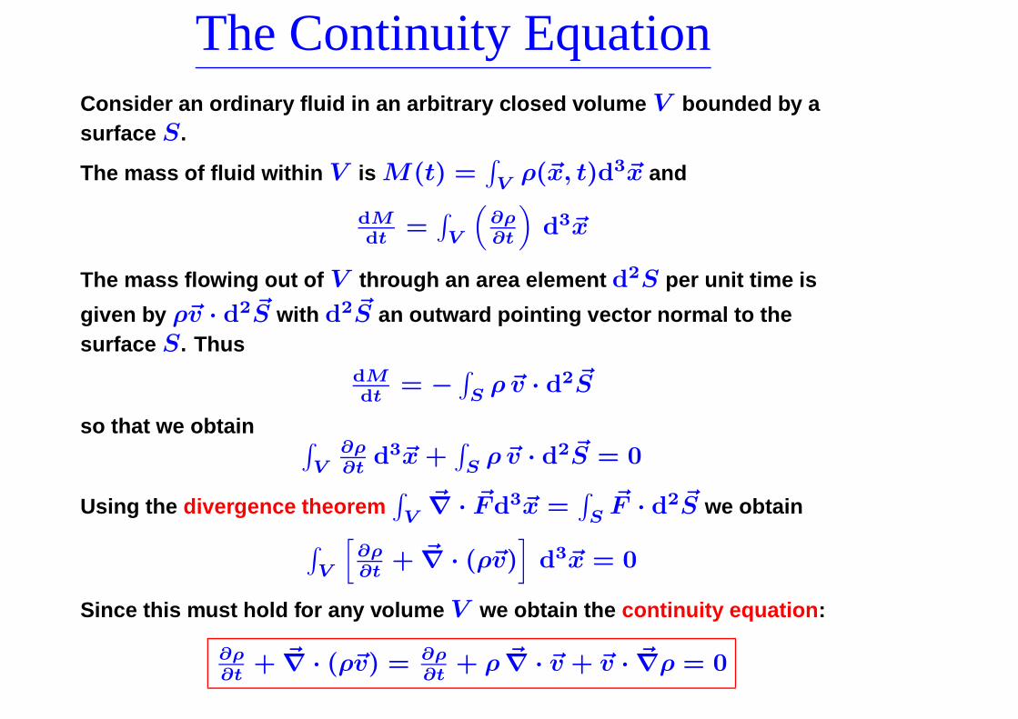
The Continuity EquationConsider an ordinary fluid in an arbitrary closed volume V bounded by asurface S.

The mass of fluid within V is M(t) =∫

Vρ(~x, t)d3~x and

dMdt

=∫

V

(

∂ρ∂t

)

d3~x

The mass flowing out of V through an area element d2S per unit time is

given by ρ~v · d2~S with d2~S an outward pointing vector normal to thesurface S. Thus

dMdt

= −∫

Sρ~v · d2~S

so that we obtain∫

V∂ρ

∂td3~x +

∫

Sρ~v · d2~S = 0

Using the divergence theorem∫

V~∇ · ~Fd3~x =

∫

S~F · d2~S we obtain

∫

V

[

∂ρ∂t

+ ~∇ · (ρ~v)]

d3~x = 0

Since this must hold for any volume V we obtain the continuity equation:

∂ρ

∂t+ ~∇ · (ρ~v) = ∂ρ

∂t+ ρ ~∇ · ~v + ~v · ~∇ρ = 0

The Collisionless Boltzmann Equation ISimilarly, for our 6D flow in phase-space the continuity equation is given by

∂f∂t

+ ~∇ · (f ~w) = 0

and is called the Collisionless Boltzmann Equation (hereafter CBE).

To simplify this equation we first write out the second term:

~∇ · (f ~w) =6∑

i=1

∂(fwi)∂wi

= f3∑

i=1

[

∂vi

∂xi+ ∂vi

∂vi

]

+3∑

i=1

[

vi∂f∂xi

+ vi∂f∂vi

]

Since ∂vi/∂xi = 0 (xi and vi are independent phase-space coordinates)

and ∂vi/∂vi = ∂∂vi

(

− ∂Φ∂xi

)

= 0 (gradient of potential does not depend

on velocities), we may (using summation convention rewrite the CBE as

∂f

∂t+ vi

∂f

∂xi− ∂Φ

∂xi

∂f

∂vi= 0

or in vector notation

∂f∂t

+ ~v · ~∇f − ~∇Φ · ∂f∂~v

= 0

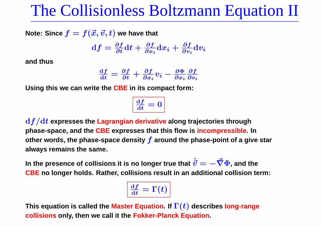
The Collisionless Boltzmann Equation IINote: Since f = f(~x, ~v, t) we have that

df = ∂f∂t

dt + ∂f∂xi

dxi + ∂f∂vi

dvi

and thusdf

dt= ∂f

∂t+ ∂f

∂xivi − ∂Φ

∂xi

∂f

∂vi

Using this we can write the CBE in its compact form:

dfdt

= 0

df/dt expresses the Lagrangian derivative along trajectories throughphase-space, and the CBE expresses that this flow is incompressible. Inother words, the phase-space density f around the phase-point of a give staralways remains the same.

In the presence of collisions it is no longer true that ~v = −~∇Φ, and theCBE no longer holds. Rather, collisions result in an additional collision term:

dfdt

= Γ(t)

This equation is called the Master Equation. If Γ(t) describes long-rangecollisions only, then we call it the Fokker-Planck Equation.

Coarse-Grained Distribution FunctionWe defined the DF as the phase-space density of stars in a volume d3~x d3~v.However, in our assumption of a smooth ρ(~r) and Φ(~r), the onlymeaningful interpretation of the DF is that of a probability density.

Note that this probability density is also well defined in the discrete case,even though it may vary rapidly. Since it has an infinitely high resolution, it isoften called the fine-grained DF.

Just as the wave-functions in quantum mechanics, the fine-grained DF is notmeasurable. However, we can use it to compute the expectation value of anyphase-space function Q(~x, ~v).

A measurable DF, one that is actually related to counting objects in a given

phase-space volume, is the so-called coarse-grained DF, f , defined as theaverage value of the fine-grained DF, f , in some specified small volume:

f(~x0, ~v0) =∫ ∫

w(~x − ~x0, ~v − ~v0) f(~x, ~v) d3~x d3~v

with w(~x, ~v) some (properly normalized) kernel which rapidly falls to zerofor |~x| > εx and |~v| > εv .

NOTE: the fine-grained DF does satisfy the CBE.NOTE: the coarse-grained DF does not satisfy the CBE.

Moment Equations IAlthough the CBE looks very simple (df/dt = 0), solving it for the DF isvirtually impossible. It is more practical to consider moment equations.

The resulting Stellar-Hydrodynamics Equations are obtained by multiplyingthe CBE by powers of velocity and then integrating over all of velocity space.

Consider moment equations related to vliv

mj vn

k where the indices (i, j, k)

refer to one of the three generalized coordinates, and (l, m, n) are integers.

Recall that

ρ =∫

f d3~v ρ〈vliv

mj vn

k 〉 =∫

vliv

mj vn

k f d3~v

The (l + m + n)th moment equation of the CBE is∫

vliv

mj vn

k∂f∂t

d3~v +∫

vliv

mj vn

k va∂f

∂xad3~v −

∫

vliv

mj vn

k∂Φ∂xa

∂f∂va

d3~v = 0

⇔ ∂∂t

∫

vliv

mj vn

k f d3~v + ∂∂xi

∫

vliv

mj vn

k vafd3~v − ∂Φ∂xa

∫

vliv

mj vn

k∂f

∂vad3~v = 0

⇔ ∂∂t

[

ρ〈vliv

mj vn

k 〉]

+ ∂∂xi

[

ρ〈vliv

mj vn

k va〉]

− ∂Φ∂xa

∫

vliv

mj vn

k∂f∂va

d3~v = 0

1st term: integration range doesn’t depend on t so ∂∂t

may be taken outside

2nd term: ∂∂xi

doesn’t depend on vi, so derivative may be taken outside.

3rd term: ∂Φ∂xi

doesn’t depend on vi, so may be taken outside.

Moment Equations IILet’s consider the zeroth moment: l = m = n = 0

∂ρ∂t

+ ∂(ρ〈vi〉)∂xi

− ∂Φ∂xi

∫

∂f∂vi

d3~v = 0

Using the divergence theorem we can write∫

∂f

∂vid3~v =

∫

fd2~S = 0

where the last equality follows from the fact that f → 0 if |v| → ∞. Thezeroth moment of the CBE therefore reduces to

∂ρ∂t

+ ∂(ρ〈vi〉)∂xi

= 0

Note that this is the continuity equation, identical to that of fluid dynamics.

Just a short remark regarding notation:

〈vi〉 =∫

vifd3~v

is used as short-hand for

〈vi(~x)〉 =∫

vi(~x)f(~x, ~v)d3~v

Thus, 〈vi〉 is a local expectation value. For brevity we do not explicitely writethe ~x-dependence.

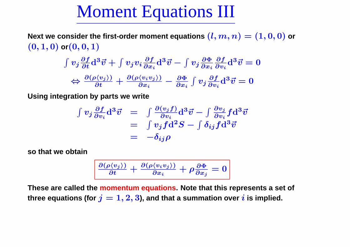
Moment Equations IIINext we consider the first-order moment equations (l, m, n) = (1, 0, 0) or(0, 1, 0) or(0, 0, 1)

∫

vj∂f∂t

d3~v +∫

vjvi∂f∂xi

d3~v −∫

vj∂Φ∂xi

∂f∂vi

d3~v = 0

⇔ ∂(ρ〈vj〉)

∂t+

∂(ρ〈vivj〉)

∂xi− ∂Φ

∂xi

∫

vj∂f∂vi

d3~v = 0

Using integration by parts we write∫

vj∂f∂vi

d3~v =∫ ∂(vjf)

∂vid3~v −

∫ ∂vj

∂vifd3~v

=∫

vjfd2S −∫

δijfd3~v

= −δijρ

so that we obtain

∂(ρ〈vj〉)

∂t+

∂(ρ〈vivj〉)

∂xi+ ρ ∂Φ

∂xj= 0

These are called the momentum equations. Note that this represents a set ofthree equations (for j = 1, 2, 3), and that a summation over i is implied.

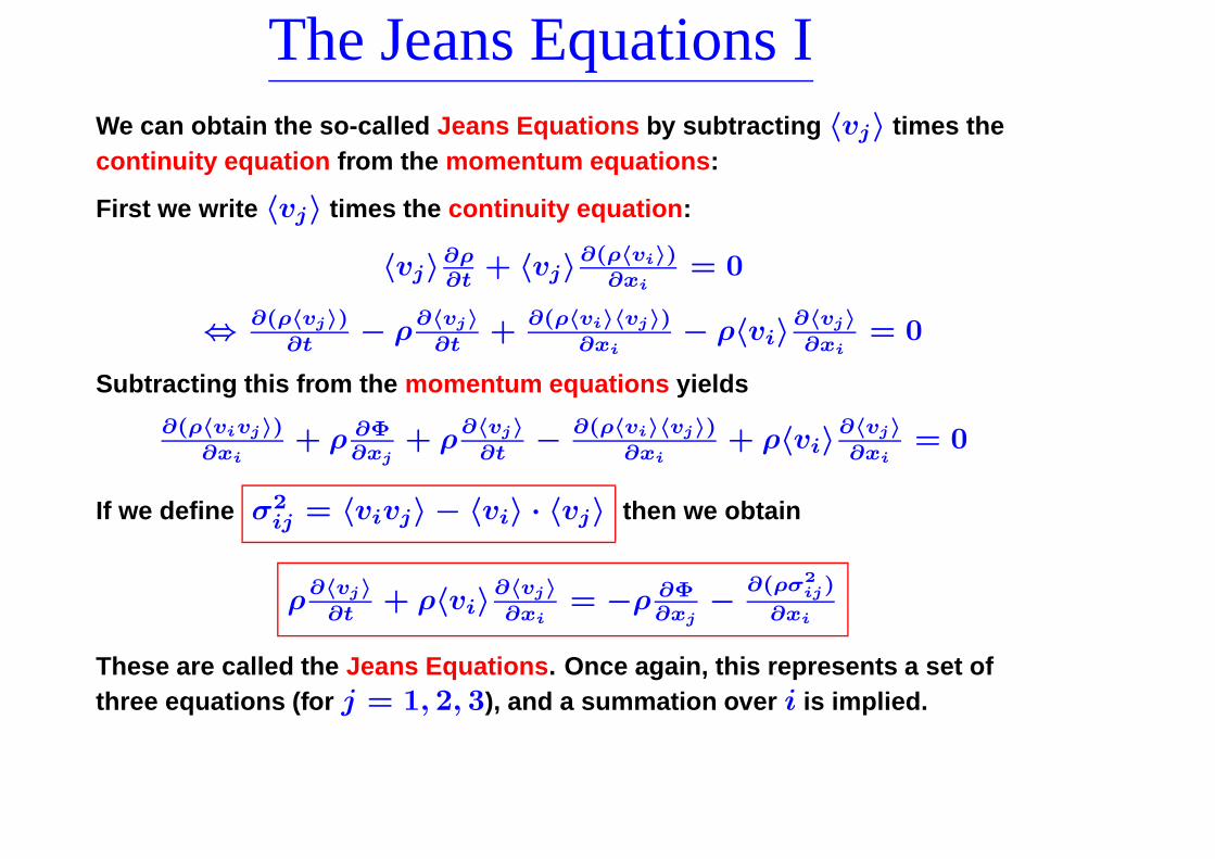
The Jeans Equations IWe can obtain the so-called Jeans Equations by subtracting 〈vj〉 times thecontinuity equation from the momentum equations:

First we write 〈vj〉 times the continuity equation:

〈vj〉∂ρ∂t

+ 〈vj〉∂(ρ〈vi〉)∂xi

= 0

⇔ ∂(ρ〈vj〉)

∂t− ρ

∂〈vj〉

∂t+

∂(ρ〈vi〉〈vj〉)

∂xi− ρ〈vi〉∂〈vj〉

∂xi= 0

Subtracting this from the momentum equations yields

∂(ρ〈vivj〉)

∂xi+ ρ ∂Φ

∂xj+ ρ

∂〈vj〉

∂t− ∂(ρ〈vi〉〈vj〉)

∂xi+ ρ〈vi〉∂〈vj〉

∂xi= 0

If we define σ2ij = 〈vivj〉 − 〈vi〉 · 〈vj〉 then we obtain

ρ∂〈vj〉

∂t+ ρ〈vi〉∂〈vj〉

∂xi= −ρ ∂Φ

∂xj− ∂(ρσ2

ij)

∂xi

These are called the Jeans Equations. Once again, this represents a set ofthree equations (for j = 1, 2, 3), and a summation over i is implied.

The Jeans Equations IIWe can derive a very similar equation for fluid dynamics. The equation ofmotion of a fluid element in the fluid is

ρd~vdt

= −~∇P − ρ~∇Φext

with P the pressure and Φext some external potential.

Since ~v = ~v(~x, t) we have that d~v = ∂~v∂t

dt + ∂~v∂xi

dxi, and thus

d~vdt

= ∂v∂t

+(

~v · ~∇)

~v

which allows us to write the equations of motion as

ρ∂v∂t

+ ρ(

~v · ~∇)

~v = −~∇P − ρ~∇Φext

These are the so-called Euler Equations. A comparison with the JeansEquations shows that ρσ2

ij has a similar effect as the pressure. However,

now it is not a scalar but a tensor.

ρσ2ij is called the stress-tensor

The stress-tensor is manifest symmetric (σij = σji) and there are thus 6independent terms.

The Jeans Equations IIIThe stress tensor σ2

ij measures the random motions of the stars around the

streaming part 〈vi〉〈vj〉.

Note that the stress-tensor is a local quantity σ2ij = σ2

ij(~x). At each point ~x

it defines the velocity ellipsoid; an ellipsoid whose principal axes are definedby the orthogonal eigenvectors of σ2

ij with lengths that are proportional to

the square roots of the respective eigenvalues.

The incompressible stellar fluid experiences anisotropic pressure-like forces.

Note that the Jeans Equations have 9 unknowns (3 streaming motions 〈vi〉and 6 terms of the stress-tensor). With only three equations, this is not aclosed set.

For comparison, in fluid dynamics there are only 4 unknowns (3 streamingmotions and the pressure). The 3 Euler Equations combined with theEquation of State forms a closed set.

The Jeans Equations IV

One might think that adding higher-order moment equations of the CBE willallow to obtain a closed set of equations. However, adding more equationsalso adds more unknowns such as 〈vivjvk〉, etc. The set of CBE momentequations never closes!

In practice one therefore makes some assumptions, such as assumptionsregarding the form of the stress-tensor, in order to be able to solve the JeansEequations.

If, with this approach, a solution is found, the solution may not correspond toa physical (i.e., everywhere positive) DF. Thus, although any real DF obeysthe Jeans equations, not every solution to the Jeans equations cprrespondsto a physical DF!!!

Cylindrically Symmetric Jeans EquationsAs a worked out example we derive the Jeans equations under cylindricalsymmetry. We therefore write the Jeans equations in the cylindricalcoordinate system (R, φ, z).

The first step is to write the CBE in cylindrical coordinates

df

dt= ∂f

∂t+ R ∂f

∂R+ φ∂f

∂φ+ z ∂f

∂z+ vR

∂f

∂vR+ vφ

∂f

∂vφ+ vz

∂f

∂vz

First we recall from vector calculus that

~v = R~eR + Rφ~eφ + z~ez = vR~eR + vφ~eφ + vz~ez

from which we obtain that

~a = d~vdt

= R~eR + R~eR + Rφ~eφ + Rφ~eφ + Rφ~eφ + z~ez + z~ez

Using that ~eR = φ~eφ, ~eφ = −φ~eR, and ~ez = 0 we have that

~a =[

R − Rφ2]

~eR +[

2Rφ + Rφ]

~eφ + z~ez

vR = R ⇒ vR = R

vφ = Rφ ⇒ vφ = Rφ + Rφ

vz = z ⇒ vz = z

Cylindrically Symmetric Jeans EquationsThis allows us to write

~a =[

vR − v2

φ

R

]

~eR +[vRvφ

R+ vφ

]

~eφ + vz~ez

Newton’s equation of motion in vector form reads

~a = −~∇Φ = ∂Φ∂R

~eR + 1R

∂Φ∂φ

~eφ + ∂Φ∂z

~ez

Combining the above we obtain

vR = −∂Φ∂R

+v2

φ

R

vφ = − 1R

∂Φ∂R

+vRvφ

R

vz = −∂Φ∂z

Which allows us to the write the CBE in cylindrical coordinates as

∂f∂t

+ vR∂f∂R

+vφ

R∂f∂φ

+ vz∂f∂z

+[

v2

φ

R− ∂Φ

∂R

]

∂f∂vR

−1R

[

vRvφ + ∂Φ∂φ

]

∂f∂vφ

− ∂Φ∂z

∂f∂vz

= 0

Cylindrically Symmetric Jeans EquationsThe Jeans equations follow from multiplication with vR, vφ, and vz andintegration over velocity space. Note that the symmetry requires that allderivatives with respect to φ must vanish.

The remaining terms are:∫

vR∂f

∂td3~v = ∂

∂t

∫

vRfd3~v = ∂(ρ〈vR〉)∂t

∫

v2R

∂f∂R

d3~v = ∂∂R

∫

v2Rfd3~v =

∂(ρ〈v2

R〉)

∂R

∫

vRvz∂f

∂zd3~v = ∂

∂z

∫

vRvzfd3~v = ∂(ρ〈vRvz〉)∂z

∫ vRv2

φ

R

∂f

∂vRd3~v = 1

R

[

∫ ∂(vRv2

φf)

∂vRd3~v −

∫ ∂(vRv2

φ)

∂vRfd3~v

]

= −ρ〈v2

φ〉

R

∫

vR∂Φ∂R

∂f∂vR

d3~v = ∂Φ∂R

[

∫ ∂(vRf)∂vR

d3~v −∫

∂vR

∂vRfd3~v

]

= −ρ∂Φ∂R

∫ v2

Rvφ

R∂f∂vφ

d3~v = 1R

[

∫ ∂(v2

Rvφf)

∂vφd3~v −

∫ ∂(v2

Rvφ)

∂vφfd3~v

]

= −ρ〈v2

R〉

R

∫

vR∂Φ∂z

∂f

∂vzd3~v = ∂Φ

∂z

[

∫ ∂(vRf)∂vz

d3~v −∫

∂vz

∂vRfd3~v

]

= 0

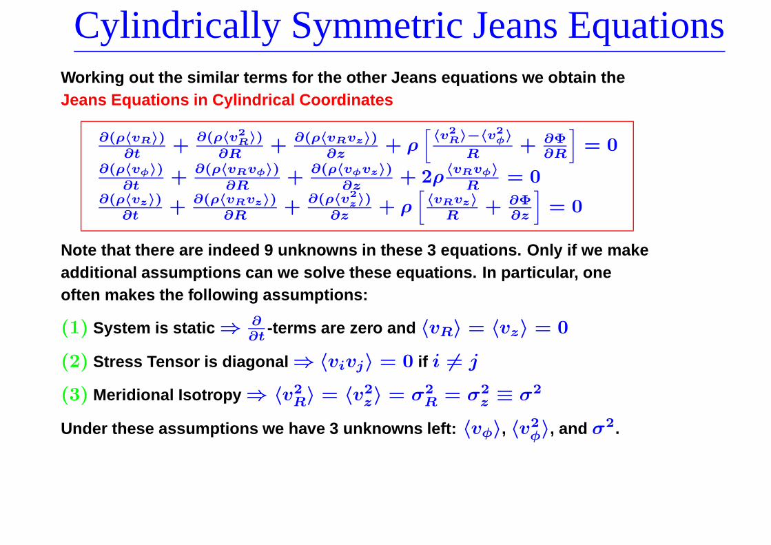
Cylindrically Symmetric Jeans EquationsWorking out the similar terms for the other Jeans equations we obtain theJeans Equations in Cylindrical Coordinates

∂(ρ〈vR〉)∂t

+∂(ρ〈v2

R〉)

∂R+ ∂(ρ〈vRvz〉)

∂z+ ρ

[

〈v2

R〉−〈v2

φ〉

R+ ∂Φ

∂R

]

= 0∂(ρ〈vφ〉)

∂t+

∂(ρ〈vRvφ〉)

∂R+

∂(ρ〈vφvz〉)

∂z+ 2ρ

〈vRvφ〉

R= 0

∂(ρ〈vz〉)∂t

+ ∂(ρ〈vRvz〉)∂R

+∂(ρ〈v2

z〉)

∂z+ ρ

[

〈vRvz〉R

+ ∂Φ∂z

]

= 0

Note that there are indeed 9 unknowns in these 3 equations. Only if we makeadditional assumptions can we solve these equations. In particular, oneoften makes the following assumptions:

(1) System is static ⇒ ∂∂t

-terms are zero and 〈vR〉 = 〈vz〉 = 0

(2) Stress Tensor is diagonal ⇒ 〈vivj〉 = 0 if i 6= j

(3) Meridional Isotropy ⇒ 〈v2R〉 = 〈v2

z〉 = σ2R = σ2

z ≡ σ2

Under these assumptions we have 3 unknowns left: 〈vφ〉, 〈v2φ〉, and σ2.

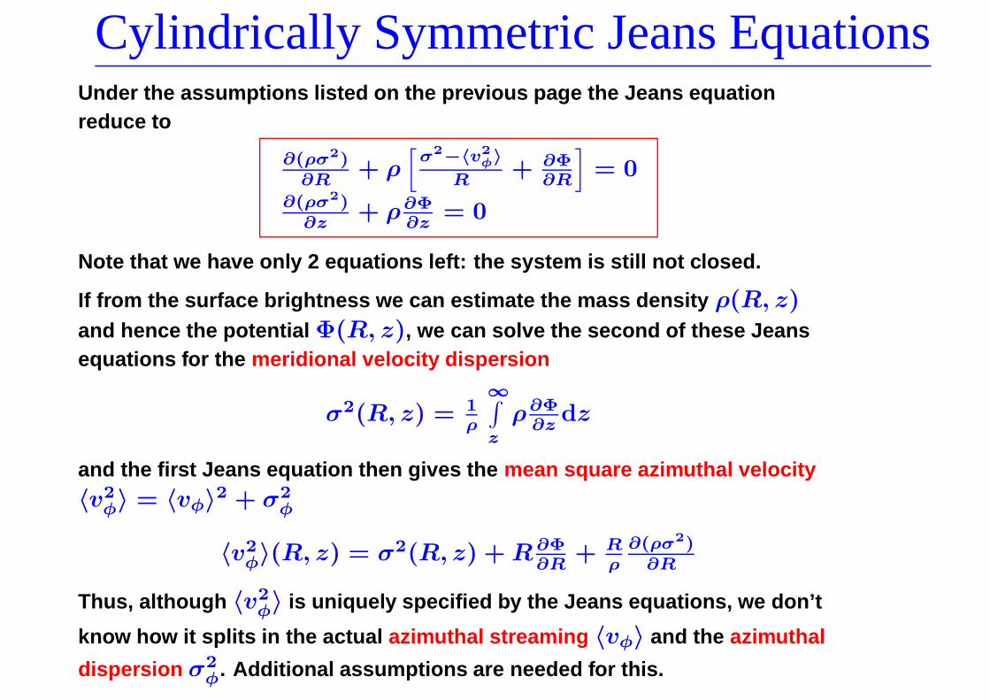
Cylindrically Symmetric Jeans EquationsUnder the assumptions listed on the previous page the Jeans equationreduce to

∂(ρσ2)∂R

+ ρ[

σ2−〈v2

φ〉

R+ ∂Φ

∂R

]

= 0

∂(ρσ2)∂z

+ ρ∂Φ∂z

= 0

Note that we have only 2 equations left: the system is still not closed.

If from the surface brightness we can estimate the mass density ρ(R, z)and hence the potential Φ(R, z), we can solve the second of these Jeansequations for the meridional velocity dispersion

σ2(R, z) = 1ρ

∞∫

z

ρ∂Φ∂z

dz

and the first Jeans equation then gives the mean square azimuthal velocity〈v2

φ〉 = 〈vφ〉2 + σ2φ

〈v2φ〉(R, z) = σ2(R, z) + R∂Φ

∂R+ R

ρ

∂(ρσ2)∂R

Thus, although 〈v2φ〉 is uniquely specified by the Jeans equations, we don’t

know how it splits in the actual azimuthal streaming 〈vφ〉 and the azimuthal

dispersion σ2φ. Additional assumptions are needed for this.

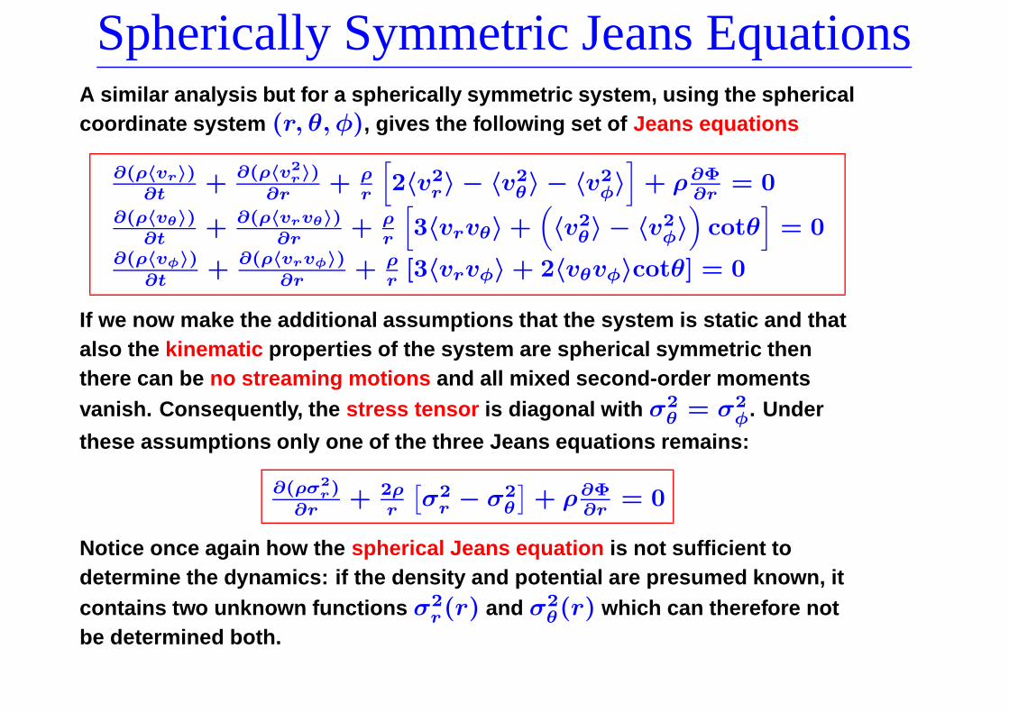
Spherically Symmetric Jeans EquationsA similar analysis but for a spherically symmetric system, using the sphericalcoordinate system (r, θ, φ), gives the following set of Jeans equations

∂(ρ〈vr〉)∂t

+∂(ρ〈v2

r〉)

∂r+ ρ

r

[

2〈v2r〉 − 〈v2

θ〉 − 〈v2φ〉

]

+ ρ∂Φ∂r

= 0

∂(ρ〈vθ〉)∂t

+ ∂(ρ〈vrvθ〉)∂r

+ ρr

[

3〈vrvθ〉 +(

〈v2θ〉 − 〈v2

φ〉)

cotθ]

= 0∂(ρ〈vφ〉)

∂t+

∂(ρ〈vrvφ〉)

∂r+ ρ

r[3〈vrvφ〉 + 2〈vθvφ〉cotθ] = 0

If we now make the additional assumptions that the system is static and thatalso the kinematic properties of the system are spherical symmetric thenthere can be no streaming motions and all mixed second-order momentsvanish. Consequently, the stress tensor is diagonal with σ2

θ = σ2φ. Under

these assumptions only one of the three Jeans equations remains:

∂(ρσ2

r)

∂r+ 2ρ

r

[

σ2r − σ2

θ

]

+ ρ∂Φ∂r

= 0

Notice once again how the spherical Jeans equation is not sufficient todetermine the dynamics: if the density and potential are presumed known, itcontains two unknown functions σ2

r(r) and σ2θ(r) which can therefore not

be determined both.

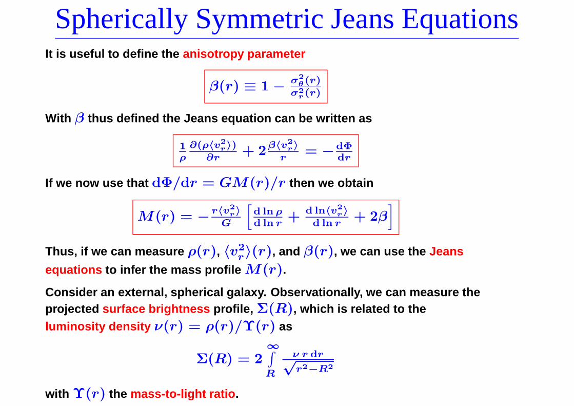
Spherically Symmetric Jeans EquationsIt is useful to define the anisotropy parameter

β(r) ≡ 1 − σ2

θ(r)

σ2r(r)

With β thus defined the Jeans equation can be written as

1ρ

∂(ρ〈v2

r〉)

∂r+ 2

β〈v2

r〉

r= −dΦ

dr

If we now use that dΦ/dr = GM(r)/r then we obtain

M(r) = −r〈v2

r〉

G

[

d ln ρ

d ln r+

d ln〈v2

r〉

d ln r+ 2β

]

Thus, if we can measure ρ(r), 〈v2r〉(r), and β(r), we can use the Jeans

equations to infer the mass profile M(r).

Consider an external, spherical galaxy. Observationally, we can measure theprojected surface brightness profile, Σ(R), which is related to theluminosity density ν(r) = ρ(r)/Υ(r) as

Σ(R) = 2∞∫

R

ν r dr√r2−R2

with Υ(r) the mass-to-light ratio.

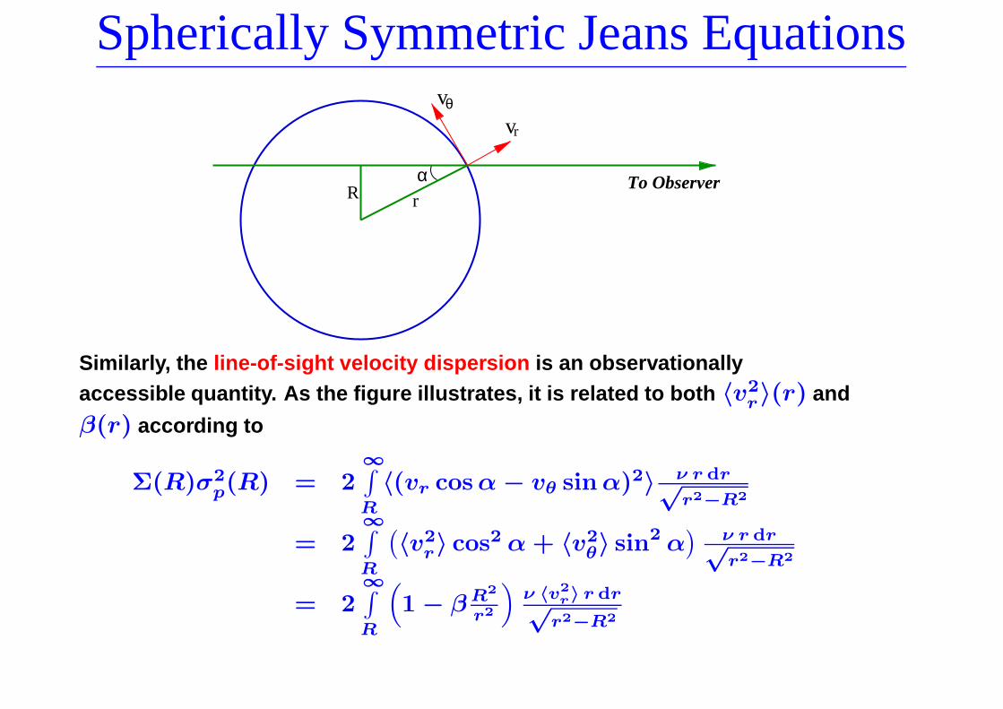
Spherically Symmetric Jeans Equations

v

R r

vθ

r

α To Observer

Similarly, the line-of-sight velocity dispersion is an observationallyaccessible quantity. As the figure illustrates, it is related to both 〈v2

r〉(r) and

β(r) according to

Σ(R)σ2p(R) = 2

∞∫

R

〈(vr cos α − vθ sin α)2〉 ν r dr√r2−R2

= 2∞∫

R

(

〈v2r〉 cos2 α + 〈v2

θ〉 sin2 α)

ν r dr√r2−R2

= 2∞∫

R

(

1 − β R2

r2

)

ν 〈v2

r〉 r dr√r2−R2

Spherically Symmetric Jeans EquationsThe 3D luminosity density is trivially obtained from the observed Σ(R):

ν(r) = − 1π

∞∫

r

dΣdR

dR√R2−r2

In general, we have three unknowns: M(r) (or equivalently ρ(r) or Υ(r)),

〈v2r〉(r) and β(r).

With our two observables Σ(R) and σ2p(R) these can only be determined if

we make additional assumptions.

EXAMPLE 1: Assume isotropy (β(r) = 0). In this case we can use the Abelinversion technique to obtain

ν(r)〈v2r〉(r) = − 1

π

∞∫

r

d(Σσ2

p)

dRdR√

R2−r2

and the enclosed mass follows from the Jeans equation

M(r) = −r〈v2

r〉

G

[

d ln νd ln r

+d ln〈v2

r〉

d ln r

]

Note that the first term uses the luminosity density ν(r) rather than the

mass density ρ(r), because σ2p is weighted by light rather than mass.

Spherically Symmetric Jeans EquationsThe mass-to-light ratio now follows from

Υ(r) = M(r)

4πR

r

0ν(r) r2 dr

which can be used to investigate whether system contains dark matter haloor central black hole, but always under assumption that system is isotropic.

EXAMPLE 2: Assume a constant mass-to-light ratio: Υ(r) = Υ0. In thiscase the luminosity density ν(r) immediately yields the enclosed mass:

M(r) = 4πΥ0

r∫

0

ν(r) r2 dr

We can now use the Jeans Equation to write β(r) in terms of M(r), ν(r)

and 〈v2r〉(r). Substituting this in the equation for Σ(R)σ2

p(R) allows a

solution for 〈v2r〉(r), and thus for β(r). As long as 0 ≤ β(r) ≤ 1 the

model is said to be self-consistent witin the context of the Jeans equations.

Almost always, radically different models (based on radically differentassumptions) can be constructed, that are all consistent with the data andthe Jeans equations. This is often referred to as the mass-anisotropydegeneracy. Note, however, that none of these models need to be physical:they can still have f < 0.