the development of a progressive failure model of a fiber

Grand Valley State UniversityScholarWorks@GVSU

Masters Theses Graduate Research and Creative Practice

4-2008

The Development of a Progressive Failure Model ofa Fiber-Rein forced Composite LaminaMichael MalettaGrand Valley State University

Follow this and additional works at: http://scholarworks.gvsu.edu/theses

Part of the Engineering Commons

This Thesis is brought to you for free and open access by the Graduate Research and Creative Practice at ScholarWorks@GVSU. It has been acceptedfor inclusion in Masters Theses by an authorized administrator of ScholarWorks@GVSU. For more information, please [email protected].

Recommended CitationMaletta, Michael, "The Development of a Progressive Failure Model of a Fiber-Rein forced Composite Lamina" (2008). Masters Theses.676.http://scholarworks.gvsu.edu/theses/676

http://scholarworks.gvsu.edu?utm_source=scholarworks.gvsu.edu%2Ftheses%2F676&utm_medium=PDF&utm_campaign=PDFCoverPages

http://scholarworks.gvsu.edu/theses?utm_source=scholarworks.gvsu.edu%2Ftheses%2F676&utm_medium=PDF&utm_campaign=PDFCoverPages

http://scholarworks.gvsu.edu/grcp?utm_source=scholarworks.gvsu.edu%2Ftheses%2F676&utm_medium=PDF&utm_campaign=PDFCoverPages

http://scholarworks.gvsu.edu/theses?utm_source=scholarworks.gvsu.edu%2Ftheses%2F676&utm_medium=PDF&utm_campaign=PDFCoverPages

http://network.bepress.com/hgg/discipline/217?utm_source=scholarworks.gvsu.edu%2Ftheses%2F676&utm_medium=PDF&utm_campaign=PDFCoverPages

http://scholarworks.gvsu.edu/theses/676?utm_source=scholarworks.gvsu.edu%2Ftheses%2F676&utm_medium=PDF&utm_campaign=PDFCoverPages

mailto:[email protected]

The D evelopm ent of a P rogressive F ailure M odel of a F iber-R ein forced

C om posite Lam ina

A thesis by

M ichael M aietta , M .S.E. presented A pril 2008

In p a r tia l fu lf illm e n t o f the req u irem en ts fo r the M aste r o f S c ien ce in E n g in ee rin g degree

(M ech an ica l)

A d v iso r: D r. P ram od C h ap h a lk ar

P adnos S choo l o f E n g in ee rin g & C om pu ting G rand V a lley S ta te U n iv e rs ity

M ichae l Maietta, 2008

The Development of a Progressive Failure Model of a Fiber-Reinforced Composite Lamina

APadnos College of Engineering and Computing

M.S.E Thesis Presentation by

Michael Maietta

ABSTRACT

Void formation is a common problem in many composite material manufacturing

processes. Composites fail when micro-eracks, whieh usually originate at voids,

propagate through the material. The meehanieal properties of a lamina depend not only

on the eonstituent properties, but also on the tow paeking eonfiguration, void eontent and

void distribution. This paper develops a method to determine the meehanieal properties

o f a tow and lamina and develops a progressive failure model to predict the strength o f a

lamina with varying void eontent, void distribution and tow paeking eonfiguration, using

finite element analysis.

The strength a lamina with various tow paeking eonfigurations, void eontent and void

distribution were investigated utilizing the progressive failure model. The tow paeking

configuration can affect the strength of a lamina by approximately 25 pereent. Voids

loeated near the gaps between the tows severely affeet the strength of the lamina. The

transverse stiffness of tows in a lamina also significantly affects the failure strength and

strain of the lamina.

GRANOAAlUEYS tate U n iv e r s it y

ACKNOWLEDGEMENTS

I would like to thank my family and friends for supporting me through my life.

Especially, my loving wife, Anne, for believing in me and putting up with the long hours

I have spent working on my computer.

I would like to express my sincere gratitude to Dr. Pramod Chaphalkar for his

guidance and support throughout the duration my graduate education and especially

during this project. I am grateful for the time he took to explain the topic of composite

materials and finite element analysis. I would also like to thank Dr. Anyalebechi and Dr.

Fung for taking the time to review my thesis presentation and paper.

11

TABLE OF CONTENTS

ABSTRACT.................................................................................................................................... i

ACKNOWLEDGEMENTS......................................................................................................... ii

LIST OF TABLES....................................................................................................................... vi

LIST OF FIGURES.................................................................................................................. viii

1 INTRODUCTION................................................................................................................. 1

1.1 Area of Investigation.................................................................................................... 3

2 LITERATURE REVIEW ............................................................................................... 4

2.1 Manufacturing Processes and How They Affect Void Formation......................... 4

2.2 Fiber and Tow Characteristics.................................................................................... 7

2.3 Measurement of Void Content.................................................................................... 9

2.4 Void Characteristics....................................................................................................13

2.5 Effect of Voids Mechanical Properties and Strength............................................. 16

2.6 Progressive Failure......................................................................................................23

2.7 Conclusion...................................................................................................................25

3 MODEL AND METHOD...................................................................................................26

3.1 Objectives and Scope................................................................................................. 26

3.2 Assumptions and Limitations................................................................................... 26

3.3 Model Loading............................................................................................................27

3.4 Model Geometry.........................................................................................................28

3.4.1 Tow Geometry...................................................................................................28

3.4.2 Lamina Geometry............................................................................................. 30

3.5 Finite Element Mesh & M odel.................................................................................32

111

3.6 Analysis M ethod......................................................................................................... 33

3.6.1 Calculation of Mechanical Properties............................................................. 33

3.6.2 Progressive Failure M odel................................................................................34

3.7 Model Parameters....................................................................................................... 35

4 FINITE ELEMENT M ODEL............................................................................................37

4.1 Generation of Finite Element M odel....................................................................... 38

4.1.1 M odeling............................................................................................................. 38

4.1.2 Voids....................................................................................................................44

4.1.3 Mesh Generation................................................................................................ 45

4.1.4 Tow Geometry Program ................................................................................... 46

4.1.5 Lamina Geometry Programs.............................................................................47

4.1.6 Computer Information...................................................................................... 49

4.2 Determination of Elastic Properties..........................................................................50

4.2.1 For Effective Young’s Moduli and Poisson’s R atios................................... 50

4.2.2 For Effective Shear M oduli..............................................................................61

4.3 Progressive Failure M odel......................................................................................... 69

4.3.1 Methodology.......................................................................................................69

4.3.2 Progressive Failure Program.............................................................................72

5 RESULTS AND DISCUSSION....................................................................................... 75

5.1 Material Selection, Properties and Dimensions...................................................... 75

5.2 Comparison of Mechanical Properties......................................................................79

5.2.1 Repeating Unit of Fibers inside a T ow ........................................................... 79

5.2.2 Repeating Unit of Fibers/Tows inside a Lam ina...........................................80

IV

5.2.3 Number of Samples to Be Analyzed...............................................................83

5.3 Progressive Failure Analysis Results...................................................................... 86

5.3.1 Square Tow Packing Configuration................................................................87

5.3.2 Hexagon Tow Packing Configuration........................................................... 89

5.3.3 Comparison of Different Tow Packing Configurations...............................92

5.3.4 Comparison of Graphite and Glass Fibers.....................................................94

6 CONCLUSIONS & FUTURE WORK............................................................................98

6.1 Conclusions.................................................................................................................98

6.2 Future W ork................................................................................................................99

7 REFERENCES......................................... 101

APPENDIX A: APDL PROGRAM S.....................................................................................103

Repeating Unit of Fibers within a Tow.............................................................................. 103

Lamina Geometry with Random V oids............................................................................. 105

Lamina Geometry with Center Void...................................................................................108

Lamina Geometry with Voids at Gaps............................................................................... 110

Lamina Geometry with Hexagon Packing.........................................................................113

Progressive Failure with Loading along Z-axis................................................................ 116

Progressive Failure with Loading along Y-axis................................................................ 119

Tow Stiffness Calculations..................................................................................................122

Lamina Stiffness Calculations............................................................................................ 125

Tow Shear Moduli Calculations......................................................................................... 128

APPENDIX B: t-DlSTRlBUTlON TABLE..........................................................................132

APPENDIX C: MISCALENEOUS DATA........................................................................... 133

LIST OF TABLES

Table 1-1: Common matrix and reinforcement material combinations [6].........................3

Table 2-1 : Fiber bundle dimensions of unidirectional tapes and prepregs [5]....................9

Table 2-2: Towpreg form parameters [5].................................................................................9

Table 3-1: Constituent properties of AS graphite fiber and PMR-15 matrix [11]........... 35

Table 3-2: AS graphite/PMR-15 lamina properties..............................................................36

Table 4-1: Repeating unit model sizes and analysis times.................................................. 50

Table 5-1: Fiber and Matrix Material Properties [11]..........................................................76

Table 5-2: AS graphite/PMR-15 tow and lamina properties...............................................76

Table 5-3: Dimensions of repeating unit of fibers inside a tow..........................................77

Table 5-4: Dimensions of the square packed repeating unit of tows in a lamina.............77

Table 5-5: Dimensions of the hexagon packed repeating unit of tows in a lamina......... 77

Table 5-6: Comparison of mechanical properties of the repeating unit of fibers inside a

tow using rule of mixtures and Finite Element Analysis, Vf t = 80% ............................80

Table 5-7: Comparison of the mechanical properties o f the square packed repeating unit

of fibers/tows inside a lamina using rule of mixture and finite element analysis, Vf =

81

Table 5-8: Comparison of the mechanical properties of the hexagon packed repeating

unit o f tows inside a lamina using rule o f mixture and finite element analysis, Vf =

82

Table 5-9: The values required for the student t-distribution test........................................85

VI

Table 5-10; Statistical analysis of the mechanical properties of the square packed

repeating unit of tows inside a lamina..............................................................................85

Table 5-11 : The failure results for the square packed repeating unit of tow in a lamina. 88

Table 5-12: The failure results for the square packed repeating unit of tow in a lamina. 90

Table 5-13; The failure results for the square packed and hexagon packed repeating units

of tow in a lamina with no voids.......................................................................................93

Table 5-14; The failure results for the square packed and hexagon packed repeating units

of tow in a lamina with gap voids...................................................................................94

Table 5-15; Glass fiber mechanical properties and strength [28]........................................95

Table 5-16; Tow and Lamina mechanical properties with glass fibers.............................. 95

Table 5-17: The failure results for the hexagon packed repeating units of tow in a lamina

with glass fibers and graphite fibers with no voids........................................................ 97

vn

LIST OF FIGURES

Figure 1-1; Common forms of fiber reinforcement: continuous fibers, whiskers,

particulate, and braid [5]...................................................................................................... 3

Figure 2-1: Composite void content as a function o f cure pressure [11]................................. 6

Figure 2-2: Cross-section of a graphite/epoxy lamina, displaying the tow cross-section

and packing [17].................................................................................................................... 8

Figure 2-3: Ultrasonic C-scan double through transmission technique [8]........................ 10

Figure 2-4: Diagram of (a) ultrasonic black-white C-scan and (b) amplitude scan of same

composite panel showing variation in ultrasound due to attenuation by voids and

fiber content variations in typical graphite-polymide composite [11].........................11

Figure 2-5: Correlation between void contents and absorption coefficient [4].................12

Figure 2-6: Photomicrographs showing the fiber end view of a composite with (a) 1.25,

(b) 3.9, (c) 12.1 volume % voids [11]...............................................................................14

Figure 2-7: Photomicrographs showing the fiber side view o f a composite with (a) 1.25,

(b) 3.9, (c) 12.1 volume % voids [11]...............................................................................15

Figure 2-8: ILSS as a function o f void content for 60% fiber volume fraction AS/PMR-15

unidirectional composites [11].......................................................................................... 17

Figure 2-9: Tensile strength vs. ultrasonic absorption coefficient [8]................................. 19

Figure 2-10: Schematics of voids (a) in fiber filament composite, (b) in fiber tow

reinforced composite [12].................................................................................................. 20

Figure 3-1: Transverse tensile test lamina with test coupon, loading and axis orientation

displayed...............................................................................................................................28

Vlll

Figure 3-2: Typical Elliptical Tow Cross Section..................................................................29

Figure 3-3: A elliptical tow cross section with a hexagonal packing and repeating unit

displayed...............................................................................................................................29

Figure 3-4: Hexagonal repeating unit of fiber inside a tow.................................................. 30

Figure 3-5: Tow packing configurations in a lamina with repeating units (a) square and

(b) hexagon.......................................................................................................................... 30

Figure 3-6: Square packing configuration in the repeating unit of tow inside a lamina

with (a) no voids, (b) one large center void, and (c) four voids at the gaps. The

loading is shown in the z-direction...................................................................................31

Figure 3-7: Hexagon packing configuration in the repeating unit of tow inside a lamina,

(a) no voids and (b) four voids at the gaps..................................... ............................... 31

Figure 3-8: Meshed repeating unit of fibers in a tow with hexagonal packing..................32

Figure 3-9: Meshed repeating units of tows in a lamina with (a) square packing and (b)

hexagon packing..................................................................................................................33

Figure 3-10: Resultant state of mechanical property calculations....................................... 34

Figure 4-1 : Unidirectional lamina and principal coordinate axes.......................................38

Figure 4-2: Elliptical Tow Cross Section...............................................................................39

Figure 4-3: A sample of a elliptical tow cross section with a hexagonal packing and

repeating unit displayed..................................................................................................... 39

Figure 4-4: Hexagonal (repeating) unit cell...........................................................................40

Figure 4-5: The tow distribution within a unidirectional lamina........................................42

Figure 4-6: Repeating unit o f a tow impregnated lamina.................................................... 43

Figure 4-7: SOLID 187 geometry, node locations, and the coordinate system [20].........45

IX

Figure 4-8: Meshed tow repeating unit with hexagonal packing.........................................47

Figure 4-9: Nomenclature for faces of the Finite Element Model.......................................51

Figure 4-10: Nomenclature for loading Case 1.....................................................................52

Figure 4-11 : Nomenclature for loading Case 2 .....................................................................53

Figure 4-12: Nomenclature for loading Case 3..................................................................... 54

Figure 4-13: Resultant forces and displacements..................................................................56

Figure 4-14: Boundary conditions for case Gxy..................................................................... 62

Figure 4-15: Boundary conditions for case Gxz...................................................................... 63

Figure 4-16: Boundary conditions for case G%y..................................................................... 64

Figure 4-17: Reaction forces for the case to obtain Gxy...................................................... 65

Figure 4-18: Reaction forces for the case to obtain Gxz ................................................66

Figure 4-19: Reaction forces for the case to obtain Gyz......................................................... 67

Figure 4-20: Boundary conditions for the progressive failure of a repeating unit in the z-

direction................................................................................................................................71

Figure 4-21: Progressive failure program logic flow chart...................................................74

Figure 5-1 : Models of the square packed repeating unit of tows in a lamina with (a) no

voids, (b) a center void, and (c) gap voids.......................................................................81

Figure 5-2: Models of the hexagon packed repeating unit of tows in a lamina with (a) no

voids and (b) gap voids...................................................................................................... 83

Figure 5-3: Comparison of the Progressive Failure of Three Square Packing

Configurations with Different Void Content...................................................................87

Figure 5-4: Screenshots from ANSYS of the progressive failure of the square packed

repeating unit of tows inside a lamina with a center void. The fibers are in gray and

the mesh is not shown.........................................................................................................89

Figure 5-5: Comparison of the Progressive Failure of the Two Hexagon Packing

Configurations with Different Void Content...................................................................90

Figure 5-6: Screenshots from ANSYS of the progressive failure o f the hexagon packed

repeating unit of tows inside a lamina with a no voids. The tows are shown in gray,

without mesh........................................................................................................................91

Figure 5-7: Comparison of Square and Hexagon Tow Packing Configurations with No

Voids................................................................................................................................ 92

Figure 5-8: Comparison of Square and Hexagon Tow Packing Configurations with Gap

Voids................................................................................................................................ 93

Figure 5-9: Comparison of glass fiber and graphite fiber lamina with hexagon tow

packing configurations and no voids................................................................................ 96

XI

1 INTRODUCTION

Composite materials have been popular in many industries, such as aerospace,

military, aquatic, and recreation, since the 1940’s. Historically, the concept of fiber

reinforcement is very old. There are biblical references to straw-reinforced clay bricks in

ancient Egypt. Iron rods were used to reinforce masonry in the nineteenth century,

leading to the development of steel-reinforced concrete.

Composite materials are macroscopic combinations of two or more distinct materials

that have readily discernible interfaces between them, that is, they do not dissolve or

merge completely into one another [1]. A composite material’s mechanical performance

and properties are designed to be superior to those of the constituent materials acting

independently. In the case o f fiber-reinforced composites, one phase is comprised of

fibers and the other phase is the matrix. The fibers form a discontinuous phase that is

dispersed throughout the matrix and function as the primary load- carrying members.

The fibers have excellent mechanical and thermal properties but need some mechanism,

which enable them to adhere together as one object during exposure to loads. The matrix

phase, also known as the resin, is usually made of a polymer and serves as the method to

adhere the fibers together [2]. As well as bonding the fibers together, the matrix provides

protection and support for the sensitive fibers and local stress transfer from one fiber to

another [3].

The attraction to composite materials is the great combination of high strength and

lightweight. Composite materials can be used in areas where conventional materials

would not optimally perform. Composite materials also have the flexibility that can

1

significantly decrease the number of components required by reducing the number of

fasteners, weldments, joints, and as a result a lesser assembly time. Some other

advantages o f composite materials include low coefficient of thermal expansion (CTE),

good vibrational damping, and resistance to temperature extremes, corrosion and wear.

Two-phase composite materials are generally classified into three broad categories

depending on the type, geometry, and orientation of the reinforcement phase: particulate

composite, discontinuous or sbort-fiber composites, and continuous composites.

Particulate composites consist of particles of various sizes and shapes. The particles are

randomly dispersed within the matrix. Discontinuous or sbort-fiber composites contain

short fibers or whiskers as reinforcement. The short fibers, which are usually quite long

compared with the diameter, can be either all oriented along one direction or randomly

dispersed. Continuous fiber composites contain long continuous fibers that run from one

edge of the composite to the other. The fibers can be parallel (unidirectional), can be

oriented at right angles to each other (cross-ply or woven), or can be oriented along

several directions (multidirectional). Continuous fiber composites are the most efficient

in terms of stiffness and strength, see Figure 1-1 [4].

Fiber-reinforced composites can be further classified into broad categories based on

the type o f matrix used: polymer-matrix composites (PMC), metal-matrix composites

(MMC), ceramic-matrix composites (CMC), and carbon matrix composites. Table 1-1

displays some common matrix and reinforcement combinations for a given composite

type.

Continuous fibers Discontinuous fibers, whiskers

Particles Fabric, braid, etc.

Figure 1-1; Common forms of fiber reinforcement: continuous fibers, whiskers, particulate, and braid [5].

Table 1-1 : Common matrix and reinforcement material combinations [6],

Composite Type Reinforcement Matrix

Polymer

Carbon (graphite) Polyester, epoxy, PEEKS-glass/E-glass Polyimide, epoxyKevlar (Aramid) Thermoplastics

Boron PEEK, polysulfone, epoxy, etc.

Metal

Boron AiuminumBorsic Magnesium

Carbon (graphite) TitaniumSilicon carbide/Alumina Copper

CeramicSilicon carbide Silicon carbide

Alumina AluminaSilicon nitride Glass-ceramic, Silicon nitride

Carbon Carbon Carbon

1.1 Area of Investigation

The scope of this project encompasses continuous uni-directional fiber-reinforced

polymer-based composites. The primary focus is on a single ply or lamina and the

manufacturing processes that can result in void formation within the matrix of the lamina.

An investigation will be conducted to determine how voids affect the mechanical

properties of laminae.

2 LITERATURE REVIEW

This chapter discusses the results of published studies of the effects of voids on the

mechanical properties of various types o f composite materials, void characteristics, void

content measurement, common composite manufacturing processes, carbon tows, and

progressive failure models. The behavior of fiber-resin composite systems with voids

under various loading types has been widely studied, discussed below. The void content

has an effect on composite interlaminar strength, transverse Young’s modulus. Poisson’s

ratio, shear modulus, and interlaminar fracture toughness. These, in turn, can have

considerable effects on the tensile and compressive strengths, shear strength, impact

resistance, fatigue life, and stiffness of the composite materials. Voids may also provide

paths by which air may reach fibers, resulting in either oxidation of the fibers or

degradation of the fiber matrix interface [7]. However, there is no general agreement on

the magnitude of the effect o f voids on the mechanical properties of composites [8].

Some work has been documented on the development of progressive failure models for

composite laminates. However, very little has been done on the progressive failure of

lamina with various void content and tow/fiber configurations.

2.1 Manufacturing Processes and How They Affect Void Formation

For most fiber-resin composite systems, void content is dependent on

manufacturing techniques and curing procedures. The fabrication process is one of the

most important steps in the application o f composite materials. An assortment of

manufacturing methods are available for composites, they include autoclave molding,

4

filament winding, pultrusion, resin transfer molding (RTM), and vaeuum-assisted resin

transfer molding (VARTM) [9].

Void formation in composite laminates occurs whenever volatile polymerization by

products (primarily water) are unable to escape from the laminate during the cure

process. It is normally assumed that voids are eliminated when the manufacturer’s

suggested cure schedule is closely followed. However, adherence to the manufacturer’s

cure cycle does not always guarantee void free composites [7]. Porosity is dependent on

variables such as temperature, temperature rates and pressure applied during the process.

The proper resin temperature will produce the correct resin viscosity, allowing the resin

to fully wet each of the fibers. The appropriate applied pressure pushes any air bubbles

to the surface o f the lamina [10]. A common problem in the manufacture of polymer

composites is the formation of defects such as voids, resin-rieh regions, delaminations,

foreign inclusions, crimped and distorted fibers. Voids are arguably the largest problem

because they are difficult to avoid and are detrimental to meehanieal properties [8].

Completely eliminating voids from composites produced by a full-scale production

facility may not be possible for all fiber-resin composite materials [11].

One composite manufacturing process; the preformed stack of composite plies is

placed in a pre-heated metal die mold and the cure pressure is applied to the die. The

temperature is increased at a steady rate until an optimum temperature is reached. The

temperature and pressure are held constant for a specified length of time. Figure 2-1

displays how the cure pressure affects the formation of voids within the composite. As

apparent, the void eontent increases at the low and high ends of the cure pressure range.

Many manufacturing issues contribute to the formation o f voids in composites, including

the formation o f unstable byproducts produced during the cure reaction of the polymeric

matrix, the use of high viscosity resin combined with closely packed fibers that are not

completely wetted by resin, the entrapment o f air, and fabrication accidents such as a

leaking vacuum bag or poor vacuum source [8]. At lower pressures, the void content

probably increases because the required pressure to remove the volatiles and air pockets

is lacking. At higher pressures, the volatiles and air pockets are most likely trapped

within the laminate [11]. The ideal cure pressure, which minimizes the void content,

appears to be between 1.5 and 5 MPa.

I

16

12 a

o6 _8o

8>4

oe

1—«e-0

1____

o O

00 mè 6o---A— I--------- 1-------- 1400 000 law 1600 2000

Cwo prossura, psi— L______ l_— «_J______I— 1 I

0 2 4 8 8 10 12 14Cura pfessura,

Figure 2-1: Composite void content as a function o f cure pressure [11].

Liquid composite molding (LCM) is another manufacturing process where it is found

that voids exist not only between fiber tows (macro voids), but also inside fiber tows

(micro voids) [12]. Resin transfer molding (RTM) is a common form of LCM. Poorly

wetted fibers are often the issue in LCM and pultrusion processes. The unwetted fibers

have no load carrying capacity in the transverse direction while in longitudinal direction

fibers are still effective. Fibers are often used in tows in LCM processes.

6

Resin Transfer Molding is a process in which a liquid thermoset resin is injected into

a mold cavity containing dry fabric preform. Due to relatively low injection pressure

applied in processing, it permits the use of lower cost mold [13].

Vacuum-assisted resin transfer molding (VARTM) is a manufacturing process in

many composite material applications where void content is critical. It is critical that the

manufacturer ensures good resin flow and complete wetout of the reinforcement under

vacuum pressure. Vacuum integrity is extremely critical because any leaks will introduce

air into the laminate, causing a loss of compaction and increased void content. It is

recommended that hill vacuum be maintained for a minimum of 24 hours at 22°C/72°F to

allow the system to cure to a stable condition [14].

Material type has an impact how carefully a laminate must be processed. For

instance, carbon fiber has much higher requirements with regard to processing accuracy.

Alignment inaccuracies and void content have a much higher impact on the mechanical

properties of a carbon laminate than they do on glass laminate properties. According to

Wind energy consultant Dayton Griffin of Global Energy Concepts LLC, "blades tend to

be thick and long, and the evacuation channels aren't great, leading to higher void

content." That is, as blade manufacturers move from hand lay-up to the more efficient

vacuum inhision processes, incorporating carbon becomes more difficult [10].

2.2 F iber and T ow C haracteristics

Konev et al [15] investigated the Modulus o f Elasticity o f carbon tow with VMN-4

fibers. The following specific modulus of elasticity were found for the tows 270-324

GPa before heat treatment and 360-560 GPa after heat treatment at 3000 degrees Celsius.

All samples had a linear density of 350 tex, mass in grams per kilometer.

A microscopic study revealed that fibers within a tow are arranged in bundles

looking like cylinders with an elliptical cross section. Binetruy et al [16] modeled the

tows in their study as cylindrical fibers bundled with a rectangular cross section.

According to Daniel and Ishai, fibers in composites with fiber volume ratios, above 60%,

tend to nest in near hexagonal packing [6].

Figure 2-2 displays the cross-section of a graphite/epoxy composite showing the tow

cross-section and the tow packing. The tows are flat and have an elliptical shape, the

packing of the tows looks to be a cross between square packed and hexagon packed.

Figure 2-2: Cross-section o f a graphite/epoxy lamina, displaying the tow cross-section and packing [17].

According to Volume 21 o f the ASM Handbook [5] the diameter of carbon fibers

typically ranges from 8 to 10 pm. Usually the larger the tow size the lower the cost per

pound.

Table 2-1 and Table 2-2 display fiber bundle dimensions for unidirectional tapes and

prepregs and towpreg form parameters, such as resin content and tow width. The width

o f a tow ranges from 1600 to 6400 pm.

Table 2-1 : Fiber bundle dimensions o f unidirectional tapes and prepregs [5].

Material Yield/tow Filament sizem/1% yd/U> pm pin.

CrmpbUe (1000 to 12,000 fllaments per tow) 300-1200 150-4500 5-10 200-390Fiberglass (245(k-12,240 Hlmments per tow) 490-2400 245-1200 4-13 160-510Aramid (800-3200 filaments per tow) 2000-7850 980-3900 12 470

Table 2-2: Towpreg form parameters [5].

Parameter Typical rangeStrand weight per length, g/m (lb/yd) 0.74-1.48 (0.00150-0.0030)Resin content, % 28-45Tow width, cm (in.) 0.16-0.64 (0.06-0.25)Package size, kg (lb) 0.26-4.5 (0.5-10)

2.3 Measurement of Void Content

Determination of the void content of a composite is not an easy task. Most voids are

internal and cannot be visually detected by the human eye. Even if all where detectable

by eye, counting voids would be a time consuming and inefficient task. Two vastly

different methods are employed to measure the void content within a composite:

nondestructive and destructive techniques.

Two ultrasonic nondestructive procedures are utilized to determine defects within the

composite. The two procedures are black-white C-scan and amplitude scan. One

technique o f the black-white C-scan is double through transmission, Figure 2-3. In this

technique an ultrasonic signal is sent through the specimen and reflected off a plate and

sent back through the specimen, defects present in the composite specimen cause

transmission loss. Usually, three independent scans of each plate are performed to

measure the absorption coefficient of the selected areas with approximately uniform

porosity level. The average value of these measurements is the absorption coefficient of

the samples. The ultrasonic absorption coefficient is defined as a ratio of the measured

transmission loss and the plate thickness [8].

Tmnaducer

Figure 2-3; Ultrasonic C-scan double through transmission technique [8].

The imbedded defects in the composite material cause variations in ultrasonic

attenuation. Areas of low attenuation, thus the presence o f defects, show up as white

areas in the black-white C-scan, Figure 2-4(a), and as low signal levels in the amplitude

scan. Figure 2-4(b).

The destructive technique for measuring the void content of a composite is calculated

from the measured fiber content, density values and the following equation [11]:

10

F - 1 - D (2 .1)

where Vv = void volume fraction, De = composite density, Df= fiber density, Dr

resin density, W/= fiber weight fraction, and Wr = resin weight fraction.

Exlent ot Ret. panel

Extent o f panel

(a)

Reference level (water)

10 percent increment in transmission

lu iH Jt tnni i t i i i i i i t i i i i i i iu

Figure 2-4: Diagram o f (a) ultrasonic black-white C-scan and (b) amplitude scan o f same composite panel showing variation in ultrasound due to attenuation by voids and fiber content variations in typical graphite-

p o ly m id e c o m p o s ite [11 ].

11

Fiber density values are obtained from the material’s vendor. Test specimens are cut

from a composite laminate and various standardized destructive tests are preformed to

determine the remaining variables in the equation above. The composite density and

resin density measurements are made by a water immersion technique in agreement with

ASTM D-792. The acid digestion technique (ASTM D-3171) is used to measure the

fiber content, where the matrix is digested in hot nitric acid. This procedure determines

the weight fractions of both the fiber and matrix; the difference between the sum of these

two values and the total weight of the specimen is the void weight fraction.

A correlation can be established between the void content determined by acid

digestion (ASTM D-3171) and the absorption coefficients measured in the ultrasonic C-

scan [4]. The results of this correlation can be seen in Figure 2-5 and as expected the

lower absorption levels correspond to lower void contents. A linear correlation between

porosity and absorption coefficient can be observed for laminates with a void content

range between 0 to 3.5%. Thus, greater void content causes increased ultrasonic

attenuation levels.

4.0

3.0

0.0I.a 2.0 1 2 1 4 10

oo##Ww (dBAnm)

Figure 2-5; Correlation between void contents and absorption coefficient [4].

12

All o f the void content measurement techniques above represent an average value over

the given volume. They do not provide any information on the shape, size, and

distribution o f the voids, other inspection techniques are used to determine these

parameters.

2.4 Void Characteristics

Depending on the type of manufacturing processes and the processing and material

conditions, voids differ in shape, size, and location [12]. Metallographic samples are

taken from the composite laminate to determine the void size, distribution and shape.

The samples are mounted, polished and photographed at various high magnification

levels. A magnification o f 200x allows the assessment of voids as small as the radius of a

single fiber of 7 p,m. Typical photomicrographs are displaying the fiber end view of a

composite are seen in Figure 2-6 and the fiber side view in Figure 2-7. The voids are

represented by the dark spots, holes between the fibers. The voids in Figure 2-6(c) can be

seen as circular in shape and Figure 2-7(c) shows the voids as long slits. From these

figures, it can be deduced that the voids are cylindrical in shape and located between the

plies. Another observation is that the voids seem to be randomly distributed within the

composite, not uniformly distributed as many studies assume.

13

w

Figure 2-6: Photomicrographs showing the fiber end view o f a composite with (a) 1.25, (b) 3.9, (c) 12.1volume % voids [11].

14

w

( b i

Figure 2-7: Photomicrographs showing the fiber side view o f a composite with (a) 1.25, (b) 3.9, (c) 12.1volume % voids [11].

15

Current opinion is that there are three possible configurations for voids in composites:

spherical, elliptical and cylindrical. Previous studies showed that in thermoset laminates,

voids tend to be small and spherical at low void contents (less than 1.5%) and tend to be

bigger and cylindrical at higher percentages [10].

The photomicrographs in Figure 2-6 and Figure 2-7 display what appears to be macro

voids, the small size or larger than the fibers, and many appear to occur between plies.

Voids can also occur at sizes smaller than fibers and within fiber tows, these are known

as micro voids. Fiber tows are a bundle of thousands of fiber filaments with a fiber

content of usually greater than 70 percent.

From Hamidi et al [18], the average void sizes in an E-glass/epoxy composite range

from 66.7 to 41.1 pm. Voids are seen at three different locations within molded

composites: areas rich in matrix away from fibers (matrix voids), areas rich in preform

(intra-tow voids), and transitional areas between the matrix and tows.

2.5 Effect of Voids Mechanical Properties and Strength

Bowles and Frimpong [11] studied the effect o f voids on the interlaminar shear

strength (ILSS) of polyimide matrix composite system. The Hercules AS graphite

fiber/PMR-15 composite was chosen for the study because void-free composites and

composites with varying void contents can be readily produced by using standard

specified cure cycles and varying the processing parameters. Each test specimen was cut

from unidirectional prepreg sheets that were made by drum-winding graphite fibers and

impregnating the fibers with the required amount of PMR-15 polyimide. Transverse and

longitudinal fiber directions were used in the specimens to see if the resin flow during

16

impregnation had any effect on the reproducibility of mechanical properties. The

interlaminar shear tests were made at room temperature in accordance with ASTM D-

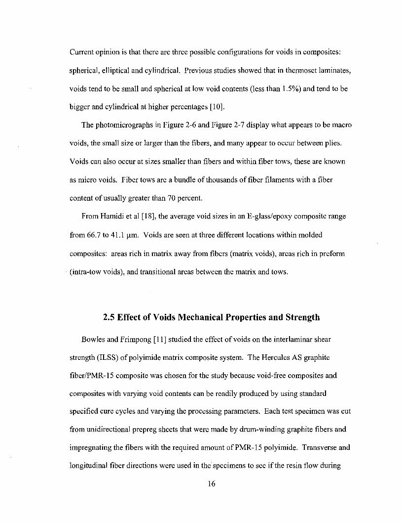
2344 by using a three-point loading fixture. Figure 2-8 displays the ILSS data for

composite with 60% fiber volume fraction with void contents determined from four

different types of data: measured, spherical void predictions, cylindrical void predictions,

and ICAN predictions. ICAN (Integrated Composite Analyzer) is a computer program

developed by Lewis Research Center for predicting composite ply properties.

Data(^lindrical voids % hedcal voids ICAN99% Confidsnce Bmits

4 6 8PwMflt voids

Figure 2-8: ILSS as a function o f void content for 60% fiber volume fraction AS/PMR-15 unidirectionalcomposites [11].

It can be seen that the spherical void prediction more closely represents the measured

data, even though the photomicrographs displayed cylindrical voids. While the

cylindrical prediction and ICAN data show lower ILSS values, cylindrical void shape

could be used for a more conservative prediction. All data measurement types display

the same trend; as the percent o f voids increase the ILSS decreases.

17

Zhan-Sheng Guo et al [8] worked toward establishing the acceptable level of defects

in a composite component, a critical issue in design. An overly conservative acceptance

criterion causes many parts that could perform satisfactorily to be unnecessarily

discarded, increasing manufacturing cost. However, an excessively liberal acceptance

criterion can result in in-service failure of some components. Both situations can be

avoided by a judicious choice, based on a reliable failure criterion, of acceptable level of

defects in the part. Interlaminar shear strength tests (ASTM D2344), flexure strength test

(ASTM D790), and tensile strength tests (ASTM D3039) were performed on 10

specimens a piece. The tensile strength tests were performed on specimens with the

dimensions of 180 x 12 x 2 mm and in an Instron mechanical testing machine with a test

speed of 0.5 mm/min. They also established a fracture criterion that correlates fracture

stress with void content, or in this case ultrasonic attenuation. They investigated

interlaminar shear strength, flexural strength, and tensile strength. The resulting failure

criterion for the strength of composite laminates containing voids is:

cr.=Hify (2 .2)

where cr^ is the fracture stress, H is the laminate toughness, a is the ultrasonic

absorption coefficient in decibels per millimeter, and m is the slope parameter. Equation

(2.2) provides a good fit to experimental results for specimens with voids. However, it

predicts infinite fracture stress for void-free laminates [8]. Therefore, for low void

contents, the fracture criterion assumes that fracture occurs according to classical fracture

18

mechanisms. Figure 2-9 displays a plot of the experimental tensile strength of laminates

with various void contents (absorption coefficient). A best fit curve and equation are

applied to the data. The best fit curve closely fits the experimental data.

1450

1350i1300

f 1250

1200

0 .8 1 .0 1 .2 1 .4 1.6 1 .8 2 .0 2 .2 2 .4 2 .6

Absorption ooefRoieot (tJB/mm)

Figure 2-9: Tensile strength vs. ultrasonic absorption coefficient [8].

It can be seen that for low void contents the tensile strength is constant and at an

absorption coefficient of approximately 1.45 dB/mm, the tensile strength begins to

decrease logarithmically. This point of slope change is the critical point, where the void

content begins to affect the laminate strength. The corresponding critical void content is

1.10percent with a toughness o f 1536 MPa and slope parameter of 0.310. This critical

value establishes an acceptance criterion for nondestructive inspection o f composite

laminates.

Yinan Wu et al [12] developed a model to estimate elastic properties o f polymer

composites with voids of various sizes and locations based on a multi level

19

homogenization procedure incorporated with the composite cylinder and Mori-Tanakan

micromechanics models [12]. The geometric model used in this method assumed

cylindrical voids imbedded in a concentric cylindrical annulus of the matrix. The elastic

properties examined were the axial and transverse Young’s modulus and axial and

transverse shear modulus. Three cases were considered voids in composites reinforced

by fiber filaments: (1) voids much smaller than fibers; (2) voids much larger than fibers;

and (3) voids surround fibers when fibers are poorly wetted. Four cases were considered

for fiber tow reinforced composites: (1) micro voids smaller than fibers; (2) micro voids

larger than fibers; (3) macro voids smaller than tows; and (4) macro voids larger than

tows. Schematics for all seven cases is displayed in Figure 2-10.

o( il ) void! smaller than filamcno (s2) voids iH jer thin filameoB

(i3) voldl luitounding filamenti (poor fiber wetting)

(bl) micro void», imiller than fibers (b2) micro voidta, luger thanfiberscro voids, lasfortft

a(b3) macro voidi, «nailer than tows (b4) macro voids, larger than lows

Figure 2-10: Schematics o f voids (a) in fiber filament composite, (b) in fiber tow reinforced composite[ 12].

In the case o f composites reinforced by fiber filaments with small voids, the content

of voids has a great influence over axial shear modulus, transverse Young’s and shear

moduli. In these three cases, the voids have a detrimental effect on these properties. The

axial Young’s modulus is unaffected by the void content. It is linearly increasing with

apparent fiber fraction and also uniformly decreasing with the increase of porosity. This

illustrates that the law of mixtures is still a good approximation for axial Young’s

20

modulus. Next, a comparison of the effect void size for small voids, large voids, and

poor fiber wetting at the same porosity was presented. The results showed that small

voids and poor fiber wetting has a larger detrimental effect on the axial shear modulus,

transverse Young’s and shear moduli than the large voids. This appears to be different

from general observations that composites with large voids degrade more in strength than

with small voids. The difference is understandable since the strength is determined by

local stress level which is intensified more by large voids while elastic properties are

determined in an average sense [12].

For the case of composites reinforced by fiber tows, voids can be found inside fiber

tows (micro voids) or between tows (macro voids). In the study, the macro and micro

voids were considered separately so the individual effects could be illustrated, even

though in actual composites they may coexist. A true volumetric fraction of fibers in

tows was set at 80 percent and porosity of 5 percent was used. The study showed that

overall, the presence of large voids appears to have a relatively small effect on the elastic

properties o f the composite, while small voids in or between fiber tows have a huge

negative effect on the elastic moduli except for axial Young’s modulus. Small voids

have the tendency to erode the binding between the tows or between the fiber filaments

inside tows. At higher fiber fractions the small voids between the tows has a very severe

effect on the transverse Young’s modulus and shear modulus and axial shear modulus.

Yinan Wu et al also conducted a finite element analysis for a rectangular composite

coupon with small voids and under unidirectional tension. Much like the case that this

paper presents. The model contained inclusions, aligned glass fibers, and voids. Using

symmetry, only a quarter of the coupon was modeled and the model was divided into 200

21

identical unit cells. A superelement was built for the unit cell and the transverse Young’s

modulus of the composite was obtained from the result of average displacements at the

ends of the tensile coupon. The finite element value was 2.303 x 10 MPa and the

predicted value from the multi level homogenization procedure was 2.376 x 10 MPa, an

error of 3.16%.

B. D. Harper et al [7] conducted a study to investigate the effects of voids upon the

hygral and mechanical properties of AS4/3502 graphite/epoxy. Uniaxial tensile

specimens with void contents ranging between 0.2% and 6% by volume were used to

determine the effect of voids upon the axial and transverse Young’s moduli, axial shear

modulus, and axial Poisson’s ratio. All specimens were tested using an MTS closed loop

hydraulic test system, the elastic moduli were determined from evaluating the slope o f the

stress-strain curve. Poisson’s ratio was determined by computing the slope o f the axial

strain vs. transverse strain plots. As the expected the axial elastic Young’s modulus and

Poisson’s ratio remains constant among the various void contents. However, the

transverse Young’s modulus and shear modulus varied a great deal between high and low

void content specimens.

The effects o f voids upon the diffusion of moisture into the test specimens were also

investigated. The presence of moisture within graphite/epoxy materials will degrade their

physical and mechanical properties. In most cases, the amount of degradation has been

found to depend primarily upon the total amount of moisture absorbed. In the study 4 ply

specimens with 1% and 5% void contents were exposed to an environment o f 24°C and

22

100% humidity. The results showed that the 5% void content specimen had a higher rate

of absorption and larger total amount of moisture absorbed.

2.6 Progressive Failure

Composite failure is not predictable with a higher reliability compared to metallic

structures due to the large number o f material parameters and structural elements that

contribute to the composite load redistribution and load carrying capability. Fracture

initiation is associated with defects such as voids, machining irregularities, stress

concentrating design features, damage from impacts with tools or other objects resulting

in discrete source damage, and non-uniform material properties stemming, for example,

from improper heat treatment. After a crack initiates it can grow and progressively lower

the residual strength of a structure to the point where it can no longer support design

loads making global failure imminent [9].

The macroscopic failure is usually preceded by an accumulation of the different types

of microscopic damage and occurred by the coalescence of the small-scale damage into

macroscopic cracks. Damage progression in a fiber-reinforced composite structure will

usually initiate by matrix cracking due to tensile stress transverse to the fiber direction

and/or additional new failures are initiated in different parts of the structure as a result of

local stress redistribution [9].

Pal and Bhattacharyya [19] conducted a progressive failure analysis on a cross-ply

laminate plate to assess the macroscopic failure criteria using the finite element method.

In the laminates the failure is must more complex than isotropic material. The weakest

ply in the laminate fails first and this failure causes a redistribution of stresses within the

23

remaining lamina of the laminate. The first ply failure does not necessarily imply the

total failure of the laminate but it is only the beginning of a progressive failure process.

If the stresses of the weakest lamina exceed the allowable strength o f the lamina, the

lamina fails which is called the first-ply failure. Each lamina is treated as homogeneous

and orthotropic in which the fibers are oriented arbitrarily. Hence, each layer is exactly

the same and the variations, such as voids, that occur in real lamina are neglected.

The methodology for this analysis is as follows the stresses and strains are calculated

for all layers, these stresses are then compared with the material allowable strength and

then failure load is determined. If the failure load of a lamina is detected, the lamina

properties are changed so that the affected stiffness of the failed lamina is discounted

completely. Displacements and stresses are recalculated and the stresses for the

remaining lamina are checked against the failure criteria to compute the failure load of

the second weakest lamina. The process continues ply-by-ply until the ultimate failure

load of a laminate is achieved.

Graphite/epoxy unidirectional laminae were used in arbitrary orientations to form a

symmetric cross-ply laminate. The maximum ultimate failure load occurs at an angular

fiber orientation of 60 degrees with a value of approximately 29 MPa x 0.001. The

ultimate failure load increases with increase in the angle of fiber orientation and number

of layer in the laminate.

24

2.7 Conclusion

It is a normal occurrence for voids to be created during the manufacture o f composite

lamina. Composite material failure tests yield varying results, presumably due to void

contents and variations in fiber packing. Micro-cracks initiate at defects such as voids,

machining irregularities and stress concentrating design features. Voids create more

significant issues than other defects because they occur internally and when the micro

cracks finally reach the surface and become visible it is too late, the material has failed.

Most examinations on the effect of voids on the mechanical properties of fiber-

reinforced polymer composites are experimental. Very little work has been completed to

develop finite element models to predict the deterioration of the strength of fiber-

reinforced polymer composites due to voids. The work that has been completed on the

progressive failure of composites usually focus on a macroscopic level, looking at the

failure of each ply in a laminate. They do not take into account the effect o f voids and

fiber packing configurations on the failure of each lamina.

An investigation should he completed to look into how voids affect the failure of

fiber-reinforced lamina using the finite element method. How do the micro-cracks

propagate through the matrix? Does the fiber or tow arrangement affect the crack

propagation? An attempt to answer these question and others will he made in this paper.

25

3 MODEL AND METHOD

3.1 Objectives and Scope

There are many different types of composite materials: polymer matrix, ceramic

matrix, metal matrix, and structural composites as discussed in chapter 1. This project

focuses on polymer matrix lamina with fiber reinforcement in the form of fiber filament

bundles called tows. The objective of this project is threefold; one is to create the tow

and lamina geometry, with or without voids and with various fiber/tow configurations

utilizing an ANSYS Parametric Design Language (APDL) program. The second

objective is use the created geometries to calculate the mechanical properties o f fiber

reinforced polymer composite lamina with various void contents and fiber/tow packing

configurations using finite element analysis. The third objective is to develop a

progressive failure model of the fiber reinforced lamina to predict the strength of

composite lamina with varying void contents and determine the mode o f failure for

various fiber/tow packing configurations using finite element analysis.

3.2 Assumptions and Limitations

The following assumptions were made in the completion of this work:

1) Fiber filaments inside the tows are packed in a hexagon configuration.

2) Tows are packed in the following configurations:

a. Square arrangement

b. Hexagon arrangement

26

3) The gaps between all tows are equal length.

4) Matrix cracks do not propagate through the tows. All cracks propagate through

the matrix and around the tows.

5) The tows are treated as homogenous solids when modeled in the repeating unit of

tows inside a lamina, the reason cracks to not propagate through the tows.

6) The interphase/interface between the fibers/tows and matrix is neglected.

3.3 Model Loading

The most critical loading of a unidirectional composite is transverse loading. This

type of loading results in high stress and strain concentrations in the matrix and

interface/interphase [6]. Thus, the choice of loading for the progressive failure analysis

was along the transverse z-axis. The orientations of the axes with respect to the lamina

geometry are shown Figure 3-1. The x-axis lies along the fiber direction, the y-axis lies

along the thickness of the lamina and the z-axis the width. The ability to complete the

progressive failure analysis with loading in the y-axis and z-axis was achieved.

However, for practical purposes the analysis was only carried out in the z direction.

Transverse tensile physical testing is normally conducted along the width of the lamina,

not the thickness. The test coupon is cut from somewhere inside of the lamina plate.

27

Coupon

►

FiberDirection

►

Figure 3-1: Transverse tensile test lamina with test coupon, loading and axis orientation displayed.

The ASTM Standard Test Method for Tensile Properties of Polymer Matrix

Composites Materials (D3039) was utilized as the testing method for the progressive

failure model. The tensile test was performed at a constant cross-speed of approximately

0.5 mm per minute, at room temperature, in the transverse direction.

3.4 Model Geometry

3.4.1 Tow Geometry

An APDL program was utilized to create the geometry of the fiber inside a tow; a tow

is a bundle of fibers with a very high fiber volume fraction, usually between 70 and 80

percent. An idealized elliptical shaped tow is utilized for geometric model. The ellipse is

comprised o f the major radius, a, and minor radius, b, displayed in Figure 3-2. The

flatness ratio of the ellipse is defined as the ratio of the minor radius to major radius.

2 8

a

Figure 3-2: Typical Elliptical Tow Cross Section.

The fibers inside a tow are usually packed in a hexagon pattern to achieve the high

fiber volume fraction, Figure 3-3.

Fiber

% $# - K - # %

Matrix

Repeating unit H exagon Pattern

Figure 3-3: A elliptical tow cross section with a hexagonal packing and repeating unit displayed.

The repeating unit is the simplest model that can be formed to represent the cross

section and is very useful for element modeling and analysis. Figure 3-4 displays the

hexagonal unit cell that was used in the model o f the tow.

29

Figure 3-4: Hexagonal repeating unit o f fiber inside a tow.

3.4.2 Lamina Geometry

Two tow packing configurations were used in the determination of the lamina

geometry, square and hexagon. The square and hexagon tow packing configuration in a

lamina can be seen in Figure 3-5.

Tow

Tow

Repeating unit

Matrix

Matrix

Repeating unit

(b)

Figure 3-5: Tow packing configurations in a lamina with repeating units (a) square and (b) hexagon.

30

( c )

Figure 3-6: Square packing configuration in the repeating unit o f tow inside a lamina with (a) no voids, (b) one large center void, and (c) four voids at the gaps. The loading is shown in the z-direction.

( a )

(b)

Figure 3-7; Hexagon packing configuration in the repeating unit o f tow inside a lamina, (a) no voids and(b) four voids at the gaps.

31

3.5 Finite Element Mesh & Model

There are two finite element models that are created in ANSYS using APDL code:

one of a repeating unit of fibers in a tow and one of a repeating unit of tows in a lamina.

Each of the repeating unit geometries was meshed with three-dimensional 10-node

tetrahedral structural solid elements, SOLID 187. The repeating unit of fibers in a tow,

Figure 3-4, was used to calculate the mechanical properties o f a tow. The mesh used for

this calculation is displayed in Figure 3-8.

Figure 3-8: Meshed repeating unit o f fibers in a tow with hexagonal packing

The tow properties calculated using the model and mesh above are used in the two

repeating unit of tows in a lamina finite element models. These models were used to

calculate the mechanical properties of the lamina and for the progressive failure model.

The mesh of the tow repeating units of tows in a lamina are presented in Figure 3-9.

32

(a)

(b)

Figure 3-9: Meshed repeating units o f tows in a lamina with (a) square packing and (b) hexagon packing.

3.6 Analysis Method

3.6.1 Calculation of Mechanical Properties

The mechanical properties, Young's Modulus and Poisson’s ratio, of the repeating

units were calculated utilizing a iso-strain superposition technique. A unit displacement

is applied at one face while the other faces are constrained so that they do not move and

33

remain planar. The reaction forces are obtained from each face. This process is repeated

on each of the other two faces and the results are superposed on each other, Figure 3-10.

The a and b constants are calculated such that two of the faces are stress free while the

other face is in uni-axial tension. The mechanical properties are calculated using the

simple stress-strain relations.

F y = F y i + a * F y 2 + b * F y 3 = 0

u = u„ + 0 + 0

Li L = F j + a * F / + b*F/ = 0

w = 0 + 0 + b*w^

------------------►

Figure 3-10: Resultant state o f mechanical property calculations.

3.6.2 Progressive Failure Model

The objective of the progressive failure model is to determine a correlation between

void content, void location, tow packing configuration, and lamina strength by subjecting

the repeating imit of tow inside a lamina to an incremental displacement, determined

from the strain rate of ASTM D3039. The progressive failure model will be applied to

loading transverse to the fibers in the z-direction. The x-direction progressive failure will

34

not be investigated because the strength in that direction is fiber dominated and the voids

have little or no effect.

Figure 3-1 displays the lamina subjected to loading in the z-direction. Boundary

conditions for the repeating unit were developed so that the faces perpendicular to the

loading (x and y) are stress free. Figure 3-6 and Figure 3-7 display how the loading is

applied to each of the repeating units. The incremental displacement is continuously

applied until the cross section of the repeating unit fails. At each loading cycle, the

reaction force on the face opposite the loading is obtained and the stress in the cross

section is calculated. A comparison of the failure stress and failure strain will be made

between the various tow packing configurations and void contents.

3.7 Model Parameters

Hercules AS graphite fiber and PMR-15 polyimide matrix were selected as the

composite materials for this study. The constituent properties are displayed in Table 3-1.

Table 3-1: Constituent properties o f AS graphite fiber and P M R -15 matrix [11].

AS Graphite FiberLongitudinal Young’s modulus Elf (GPa) 213.7Transverse Young’s modulus Ezf (GPa) 13.7Axial shear modulus G,2f (GPa) 13.7Transverse shear modulus Gz3f (GPa) 6.8Poisson’s ratio Vl2f 0.3T e n s i le S tr e n g th CTyr (M P a ) 3 0 3 3 .8

Density 8f (g/cm^) 1.799PMR-15 Matrix

Young’s modulus Em (GPa) 3.2Shear modulus Gm (GPa) 1.1Poisson’s ratio Vm 0.36Tensile Strength aim (MPa) 55.8Density 5m (g/cm^) 1.313

35

Some other properties of a common AS graphite/PMR-15 lamina are required for the

analysis, Table 3-2, such as the fiber diameter [4], tow and lamina fiber volume ratios,

tow flatness ratio and the number o f fibers within a tow.

Table 3-2: AS graphite/PMR-15 lamina properties.

Graphite fiber diameter df (pm) ‘ 7Tow fiber volume ratio Vf,t 0.80Lamina fiber volume ratio Vf 0.50Number of fibers per tow 3000Tow flatness ratio (b/a) fr 0.10

The void sizes used in the generation o f the lamina repeating units were based the

geometric and finite element model limitations. A maximum void diameter of 50

microns was chosen based on the information from reference [18]. The location chosen

for the voids was between the tows. For reference [12] it was determined that the small

voids (smaller than the tows) had a larger effect on the performance of the composite

than larger voids.

The topics covered in this section are discussed in detail in chapter 4 with the results

of the analysis presented in chapter 5.

36

4 FINITE ELEMENT MODEL

A lamina is a sheet or ply of unidirectional fiber-reinforced composites and multiple

layers o f lamina are stacked in various angular arrangements to form a multi-directional

laminate. The reinforcement can come in the form of individual fiber or bundles of

thousands of fiber, called tows. When multi-directional laminates are use in structural

applications, accurate predictions of elastic properties such as the Young’s and Shear

moduli and Poisson’s ratios are desirable. To determine the elastic properties of the

laminate the elastic properties of the individual lamina must be known. The presence of

voids within the matrix of a lamina can have a detrimental effect the elastic properties

and thus, the elastic properties of a lamina with voids must be determined. Voids can

also affect the failure mode of the lamina, as the voids act as stress risers. It is important

to know how and to what extent do the voids affect the properties and strength of the

lamina. Finite element modeling can be an effective tool used to predict these properties

and evaluate the progressive failure of the lamina. As seen in the previous section much

work has been done covering this topic, with the majority focusing on the interlaminar

shear strength of a laminate. In addition, most of the research has been completed

experimentally with very little utilizing finite element analysis. This focus here is the use

of Finite Element Analysis to determine the effect of voids on the elastic properties and

strength of a lamina.

37

4.1 Generation of Finite Element Model

All modeling and analysis were completed in ANSYS 11.0, utilizing the ANSYS

Parametric Design Language (APDL). Modeling techniques and mesh generation for the

repeating unit of the unidirectional lamina is presented. A finite element model is

developed for determination of macroscopic mechanical properties.

4.1.1 Modeling

The geometrical structure of a unidirectional lamina is simple. A lamina (ply)

consists of matrix containing tows (bundles of fibers), oriented in one direction. The

lamina is an orthotropic material with principal material axes in the direction of the tows,

normal to the tows in the plane of the lamina, and normal to the plane of the lamina [6],

Figure 4-1 displays the principal axes o f a unidirectional lamina. In the model, principal

axis 1 coincides with the x-axis, axis 2 with the z-axis, and axis 3 with the y-axis.

Figure 4-1: Unidirectional lamina and principal coordinate axes.

38

Repeating Unit o f Fibers Inside The Tow

An idealized elliptical shaped tow is utilized for geometric model. The ellipse is

comprised of the major radius, a, and minor radius, b, displayed in Figure 4-2.

Figure 4-2; Elliptical Tow Cross Section.

A tow is a bundle of fibers with a very high fiber volume fraction, usually between 70

and 80 percent. In order to obtain this high of a fiber volume fraction the fibers are

packed in a hexagonal pattern. It is assumed that all of the fibers are of equal size and

spacing is held constant. In reality, the diameters o f the fibers vary slightly and the

proper spacing is not always held true. For this type of cross section, a simple hexagonal

pattern and repeating unit can be identified, as shown in Figure 4-3.

Fiber Matrix

R ep ea tin g unit H ex a g o n P attern

Figure 4-3: A sample o f a elliptical tow cross section with a hexagonal packing and repeating unitdisplayed.

39

The repeating unit is the simplest model that can be formed to represent the cross section

and is very useful for element modeling and analysis. This allows for smaller and an

increase number of elements to be used, which will improve the results o f the analysis.

Figure 4-4 displays the hexagonal unit cell that was used in the model of the tow. In

order to model the unit cell its dimensions must be determined. Triangle kmn is an

equilateral triangle with leg length c. The unit cell is rectangular with side lengths, c and

Wu, fiber radius, r/, and tow fiber volume fraction, Vf t-

Li

mC

V

n

Figure 4-4: Hexagonal (repeating) unit cell.

The fiber radius and tow fiber volume fraction are known quantities, while the side

lengths are unknown. The fiber volume fraction is defined as:

^ f l b e r _ 27# /

CW,(4.1)

where Afiher is the fiber area and Au is the total unit cell area. From triangle kmn the

width, Wu, is calculated and the height, c, is calculated using equation 4.1 :

40

w„ = VSc

" 2®-; (4 2)

The length of the model was determined to not have an effeet on the analysis results

and was ehosen at a length to ease the amount of eomputer resourees required to run the

analysis.

Lamina Repeating Unit Model

The dimensions, a and b, of the elliptical tow, see Figure 4-2, are unknown and must

be determined. Using the following relations the can be determined.

^ f i b e r ~

/ '- = % (4.3)

Nrirl , -Aow = = m h ^ 7 ta

* f

where N is the total number of fibers in a iov>/,fr is the flatness ratio (aspect ratio) and Vf

is the overall fiber volume fraction in the lamina. The following quantities are known:

total number of fiber in tow, N, and the aspect ratio. And finally, a and b are

determined;

41

a =y r x / r

b = a x f r

(4.4)

The tows within a laminate are distributed uniformly throughout the cross section.

The packing is similar to that of a simple cubic; except instead of circular fiber there are

elliptical tows, see Figure 4-5.

MatrixT ow

R ep ea tin g unit

Figure 4-5: The tow distribution within a unidirectional lamina.

The repeating unit of the tow lamina contains a quarter of an elliptical tow at each comer

of the rectangular unit. The elliptical shaped tows allow for tighter packing in the lamina,

increasing its stiffness and strength. Figure 4-6 displays the repeating unit of a tow-

impregnated lamina with height h, width w and gaps g on the top, bottom and side faces.

42

Gap-^ I**-l i

_ j L

T "G ap

-w -

Figure 4-6; Repeating unit o f a tow impregnated lamina.

The assumption is that both gaps are of equal length. With a and b already know the

dimensions of the repeating unit can be calculated.

w - 2a + g h = 2b + g (4.5)Aom — W X h xV ^ — N X

where Aiam is the area of fibers in within the lamina repeating unit. The equation above

can be rearranged into the following quadratic equation;

g^ + 2 ^ + b + 4ab -NA fiber

= 0 (4.<%/ y

Solving for g using the quadratic formula:

43

g = - ( a + 6) ± ii + bVf

04 7)

The length o f the model was determined to not have an effect on the analysis results

and was chosen at a length to ease the amount o f computer resources required to run the

analysis.

4.1.2 Voids

Voids were neglected in the repeating unit o f fibers inside a tow. This project is

concerned with the voids located around the tows in the lamina. The voids in the lamina

are small macro voids, smaller than the tows and located between and around the tows.

The number and size of the voids determine the void content of the repeating unit of the

tows inside the lamina, it was desired to produce geometries with various void contents

with various void locations and geometries where the void locations and sizes are user

defined.

Demma and Djordjevice [10] presented in thermoset matrix laminates the voids tend

to be spherical in shape. Since, a thermoset matrix was selected for the model, the voids

are modeled as spheres.

The void content of the repeating unit o f the tows inside the lamina unit with

sp h erica l v o id s is ca lcu la ted u sin g the eq u ation s 4 .8 .

44

== tv X A X

(4.8)

= ^ x I O Ototal

where Vtotai is the total volume of the repeating unit, Vvou is the total volume of the voids,

ry is the void radius, and Vconiem is the void volume fraction.

4.1.3 Mesh Generation

The element choice for the model’s mesh is SOLID 187, a three-dimensional 10-node

tetrahedral structural solid, with each of the 10 nodes having three degrees of freedom:

translations in the nodal x, y, and z directions. SOLID 187 has a quadratic displacement

behavior and is well suited to modeling irregular meshes. It is also good for curved

boundaries, such as around the voids and fibers. The geometry, node locations, and

coordinate system are shown in Figure 4-7.

Y

Figure 4-7: SOLID 187 geometry, node locations, and the coordinate system [20].

45

The size of the mesh was determined using the SMRTSIZE command. This

command allows ANSYS to automatically determine the size of each element based on

the geometry. The smallest element size was used for the mesh, in most cases the finer

the mesh the better the results. To avoid element errors (i.e. tetrahedrons with

straightened edges, inverted Jacobian determinant, and small interior angles) the

tetrahedron element improvement option, MOPT, was utilized. The improvement occurs

through the use of face swapping and node smoothing techniques. Finally, the geometry

was meshed using the free mesh command.

4.1.4 Tow Geometry Program

A program was developed utilizing the ANSYS Parametric Design Language to

create the tow repeating unit geometry, Tow_repeating_unit.txt is located in Appendix.

ANSYS Parametric Design Language (APDL) is a scripting language that can be used to

automate common tasks or build the solid model in terms of parameters. The list of

commands can be written as a macro in a text file and imported in ANSYS or each

individual command can be entered into the dialog box.

The inputs to the program are the fiber radius, height of unit cell, width of unit cell,

length, and material properties. The dimensions of the tow repeating unit are calculated

in a spreadsheet using the equations discussed above and the material properties for the

individual fibers and matrix were obtained from Bowles and Frimpong [11]. From these

parameters the void-free repeating unit geometry is produced by first creating the

rectangular matrix and then the circular fibers. The matrix volume that is overlapped by

the cylindrical fiber is subtracted and the remaining volumes are glued together. Finally

46

the volumes are meshed with the SOLID 187 elements producing the tow repeating unit,

Figure 4-8.

Figure 4-8: Meshed tow repeating unit with hexagonal packing.

4.1.5 Lamina Geometry Programs

Four programs were developed to create four different lamina repeating unit

geometries. The first three created a cubic type cross section with varying void contents

and the fourth program created a hexagonal cross section. All four programs are located

in the Appendix.

Random Void Generation

This program, Lamina_Geometry_Random.txt, is capable of creating a void free

lamina or a lamina with random void content. The inputs to the program are the tow

major and minor radii, tow aspect ratio, lamina repeating unit height, width, length, and

mechanical properties. The mechanical properties o f the lamina were calculated using

the tow repeating unit program and input into this program. From these parameters the

47

repeating unit geometry is produced by first creating the rectangular matrix and then the

elliptical tows. The elliptical volume is not a readily available command in ANSYS;

some manipulation of a cylinder was necessary to achieve the appropriate shape.

Utilizing the volume scale command (VLSCAL) and the tow aspect ratio, the cylinder

was flattened into an elliptical volume. The matrix volume that is overlapped by the

elliptical tows is subtracted and the remaining volumes are glued together.

At this point a decision must be made, “Do you want to create voids?” If the answer

is “No” the program continues on and meshes the volume. If the answer is “Yes” the

program continues to the void creation loop. Five random numbers are generated in the

program; a random integer to represent the number of voids, a number between zero and

the maximum void radius to represent the radius o f one void, and the x, y, and z locations

o f the void. The x, y and z locations are limited so that the voids are only created within

the matrix. To create a void the program generates a spherical volume and that volume is

subtracted from the matrix, leaving a “void” of material. The program continues to loop

through until the correct number of voids is created. Following the completion of the

geometry, the geometry is meshed. The output of the program in addition to the meshed

geometry is the number of voids created, the total volume of the voids, and the void

content of the geometry.

User-defined Void Locations

The other two programs create the void free lamina repeating unit geometry in the

exact same method as the random program. The difference is that instead of randomly

generated voids, the user determines the locations o f the voids. Program

48

Lamina_Geometry_center.txt creates one large void in the exact center of the model.

Program Lamina_Geometry_gap.txt creates four voids, all at the mid-plane in the x

direction, two large voids near the top and bottom gaps and two small voids at the side

gaps.

Hexagonal Tow Packing

Another tow packing configuration can be model to determine the mode of failure

due to transverse tensile loading. The tows are orientated in a hexagonal pattern similar

to the arrangement of fibers within a tow. This program also contains the ability for the

user to create voids at specified locations.

4.1.6 Computer Information

This section contains the computer specifications used for the analysis, model sizes,

and approximate length of computation time. A computer with the following

specifications was used for the ANSYS analysis:

Dell Inspiron E l505 Laptop

Intel CPU T2300 @ 1.66 GHz

1.0 GB of RAM

The table below contains the number of nodes, number of elements, and approximate

analysis times for each of the repeating unit (RU) models.

49

Table 4-1: Repeating unit model sizes and approximate analysis times.

Model Type # of Nodes # of Elements Analysis Time (min.)Tow RU 24,805 16,777 30Square Lamina RU - No Voids 14,220 8,417 25Square Lamina RU - Center Void 22,796 14,419 40Square Lamina RU - Gap Voids 31,506 19,659 50Hexagon Lamina RU - No Voids 29,318 17,716 45Hexagon Lamina RU - Gap Voids 60,463 39,363 75

4.2Determination of Elastic Properties

This chapter describes in detail the methodology used to formulate the tests and

calculate the effective Young’s moduli, Poisson’s ratios, and shear modulus o f the tow

repeating unit and the lamina repeating unit. The sections below detail how the elastic

properties of the tow repeating unit is calculated, the elastic properties of the lamina

repeating unit are calculated in the exact same method. The only difference is the change

of the following nomenclature: = L , W u = w, and c = h. An APDL program was

developed for the computation of the elastic properties. Young’s Moduli and Poisson’s

ratios, and the shear moduli.

4.2.1 For Effective Young’s Moduli and Poisson’s Ratios

To obtain the mechanical properties for the fiber-reinforced composite unit cell, three

iso-strain boundary conditions were superimposed. The objective of the iso-strain

boundary conditions is to achieve a state of deformation where all faces remain planar

and normal to each other. Only one face, along with its opposite face, has a net force and

the remaining surfaces have a net zero force [21]. These conditions create a uniaxial

50

loading case. Poisson’s ratio can be determined by the ratio of lateral strain to axial

strain and Young’s modulus can be determined by the ratio of axial stress to axial strain.

Boundary Conditions

The three iso-strain cases are described in detail below. The nomenclature for the

faces of the finite element model is shown in Figure 4-9.

y = c Face

y = 0 Face

z = Face

z = 0 Face

Figure 4-9: Nomenclature for faces o f the Finite Element Model.

Case I: uniaxial tension in x-direction, see Figure 4-10.

Constraints'.

On X = 0 face: u = 0 and on x = Lu face: u = Ug.

On y = 0 and y = c faces: v = 0.

51

On z = 0 and z = Wu faces: w = 0.

From these constraints, the following reaction forces result.

on either x = 0 or x = Lu face.

Fy on either y = 0 or y = c face.

Fy on either z = 0 or z = Wu face.

u = 0

V = 0

u = 0

w = 0

w = 0

Figure 4-10: Nomenclature for loading Case 1

Case II: uniaxial tension in y-direction, Figure 4-11.

Constraints:

On X = 0 and x - Lu faces: u = 0.

On y = 0 face: v = 0 and on y = c face: v = v«.

On z = 0 and z = Wu faces: w =0.

52


F_ on either x = 0 or x = Lu face.


F, on either z = 0 or z = Wu face.

u = 0

w = 0

u = 0

w = 0


Case III: uniaxial tension in z-direction, Figure 4-12.

Constraints:

On X = 0 and x - Lu faces: u = 0.

On y = 0 and y = c faces: v = 0.

On z = 0 face: w = 0 and on z = Wu face: w =Wo.

53

From these restraints following reaction forces result.

F„ on either x = 0 or x = Lu face.


Fg on either z = 0 or z = Wu face.

V i 1

V = 0 fu = 0 ----------

u = 0 ---------------- ►

V - 0

t t t I T M ! fu = 0

w = 0 ^


Computation o f Elastic Properties

As stated above, the three iso-strain boundary condition cases were superimposed

using two undetermined variables, a and b. The resultant state of deformation is

Resultant state = (State of Case I) + a * (State of Case II) + 6 * (State of Case III)

54

The resultant displaeements in the x, y and z directions are, Figure 4-13:

M — Wq + 0 + 0v = 0 + a - V g + 0 (4.9)

w — 0 - f 0 - f h • W q

Henee, the three average strains of the unit cell are

(4.10)c

w . .

and the resultant forces in the x, y, z directions are displayed below and in Figure 4-13:

F ; (4.11)

55

V = 0 + a*v„ + 0 t Fy = F ; + a*F/ + b*F/

u = u„ + 0 + 0

Fx =F;+a*F / + b*F,3

Li F, = F-i + a*F 2 + b*F,3

w = 0 + 0 + b*Wg

-----►

Figure 4-13: Resultant forces and displacements

Computation o f Ex, Vxy, Vxz

To determine mechanical properties above, the resultant superposition and choice of

constants a and b are such that the resultant forces on all y and z faces are zero but are

non-zero on the x faces; Fy = 0, Fz = 0, and F% ^ 0. Thus, the stress in each direction is

defined as:

=W ..C

C7y=0

( 7 = 0

(4.12)

Therefore, it is a uniaxial loading case in the x-direction. Consequentially, the following

relations can be written.

56

w, / I ,

(4.13)g, IL„ U„w„O U

E = ^ = ^ ^ l ^ ^ = - ^ ^ l + a - F ^ + b - F lA / f ~A A Ag, U„/L U WC

From the case definition and Equation 4.11, the following relation can be achieved

F, = F^ + a • + 6 • F^ = 0

Constants a and h are determined from solving the following simultaneous linear

equations, which are obtained by rearranging Equation 4.14.

a . ( F / ) + 6 .(F ;f) = - F ;(4.15)

Thus,

(4.16)

Hence, E% , v%y and Vxz are calculated by substituting a and b in Equation 4.13.

57

Computation o f Ey, Vy , Vyz


constants a and b are such that the resultant forces on all x and z faces are zero hut are

non-zero on the y face; Fx = 0, F% = 0, and Fy ^ 0. Thus, the stress in each direction is

defined as:

cr = 0

(T (4.17)

( 7 = 0

Therefore, it is a uniaxial loading case in the y-direction. Consequentially, the following

relations can he written.

s . u^tL,, u„c

^y = — = — £— ( ; + a . f ; + i ■ F f S a - v , / c

From the case definition and Equation (4.11), the following relation can he achieved

F = F ‘ + a - F ^ + b - F ^ = 0

58

and constants a and b are determined from solving the following simultaneous linear

equations, which are obtained by rearranging Equation (4.19).

(4.20)

Thus,

X Z X z

p K p ^ _ p F p 2

y rpi 7 7 2 7 7 2 7 7 3

(4.21)

p ^ . p ^ - p ^ . p^^ X ^ Z ^ X ^ z

Hence, By , Vy% and Vyz are calculated by substituting a and b in Equation 4.18.

Computation o f E , Vzy,


constants a and b are such that the resultant forces on all x and y faces are zero but are

non-zero on the z face; Fx = Q,Fy = 0, and F^ ^ 0. Thus, the stress in each direction is

defined as:

= 0 (4.22)

59

Therefore, it is a uniaxial loading case in the z-direction. Consequentially, the following

relations can be written.

(4.23)b-w^ lw^ b- WgC

% C + a - F , ^ + 6 - F ye, b - w / w ^ 6

From the case definition and Equation (4.11), the following relation can be achieved

F, = F ! + a - F ^ + b - F ^ = 0(4.24)

F ; = F ’ + a - F + b - F ^ = 0

and constants a and b are determined from solving the following simultaneous linear

equations, which are obtained by rearranging Equation 4.24.

Thus,

60

(4.26)

Hence, Ez, Vzy, and Vzx are calculated by substituting Qz and bz in Equation 4.23.

Elastic Properties Program

Two APDL programs, Appendix, were developed to apply the iso-strain boundary

conditions to the tow repeating unit and the lamina repeating unit for each of the three

cases. The inputs into the program are the unit displacements for each of the three cases.

The program progresses through each of the three cases independently, removing the

previous cases boundary conditions before applying the new boundary conditions. The

output is the reaction forces for each of the three cases. The reaction forces from the

program were imported into a spreadsheet where the a and b constants and elastic

properties were calculated using the method discussed above.

4.2.2 For Effective Shear Moduli

To obtain the effective shear moduli, three more boundary conditions are applied to

the faces of the model remain planar to its opposite face. The shear modulus can be

determined by the ratio of shear stress to shear strain.

61

Boundary Conditions

Refer to Chapter 3 for the model geometry. The boundary conditions for the three

cases are described in detail below.

Case Gxy'.

The boundary conditions for the computation of Gxy are below, see Figure 4-14.

On y = 0 face: u = 0 and v = 0

On y = c face: u = Uo and v = 0

On X = 0 and x = Lu faces: u = Uo*(y/c) and v = 0

On z = o and z = Wu faces: w = 0

u = u * y/c) / u = Ug*(y/c)

u = 0, V = 0

Figure 4-14: Boundary conditions for case G*


F^ and F^ on y = c face

F,f and F^ on x = Lu face

F® and F® on y = 0 face

F^ and F} on x = 0 face

62

Case Gxz '

The boundary conditions for the computation o f Gxz are below, see Figure 4-15.

On z = 0 face: u = 0 and w - 0

On z = Wu face: u = Uq and w = 0

On X = 0 and x = Lu faces: u = Uo*(z/Wu) and v = 0

w = 0

u = u *(z/w^

' w = 0w = 0

/ u = u /(z /w j

u = 0, w = 0

Figure 4-15: Boundary conditions for case G%

From these constraints the following reaction forces result.

F^ and on z = Wu face

F^ and F / on x = Lu face

F® and F f on z = 0 face

Ff' and on x = 0 face

Case G,zy

The boundary conditions for the computation of Gzy are below, see Figure 4-16.

On y = 0 face: v = 0 and w = 0

On y = c face: v = 0 and w = Wo

63

On z = 0 and z = Wu faces: v = 0 and w = Wo*(y/c)

V = 0

w = w„*(y/c)

V = 0, w = 0

w = W g*(y/c)

V = 0

Figure 4-16: Boundary conditions for case

From these constraints the following reaction forces result.

and on y = c face

F ^ and on z = Wu face

F ^ and F ^ on y = 0 face

F„ and on z = 0 face

Computation o f Shear Properties

Computation o f Gxy

Refer to the reaction forces discussed above and see Figure 4-17.

64

V i

A1

i

------------

1

L- F ^ -------------- ^y ■<------------

Fx® = Fx".............. X

i F

Figure 4-17: Reaction forces for the case to obtain Gxy

It was observed from the results in ANSYS that was insignificant when compared

to F^ on the y = c face (F^ was on the order of ten thousand times greater than F^ ).

Therefore, there was only a shear force on this face. Similarly, it was observed that F^

was insignificant when compared to F^ on the x = Lu face. Therefore, there was only a

shear force on this face. It was also observed that F^ = F^ , F^ = F®, and

= Fy w 0. Hence, calculating the average shear stress on x = Lu face and y = c face

and utilizing the small angle theorem to calculate the shear strain:

V 1 A 2

+ '

01.27)

pU pR

65

Computation o f Gxz

Gxz is calculated similarly to Gxy. Refer to the reaction forces discussed above and

see Figure 4-18.

FR=(

Figure 4-18: Reaction forces for the case to obtain

It was observed from the results in ANSYS that was insignificant when

compared to on the z = d face ( F^ was on the order o f ten thousand times greater

than ). Therefore, there was only a shear force on this face. Similarly, it was

observed that F f was insignificant when compared to F f on the x = Lu face. Therefore,

there was only a shear force on this face. It was also observed that F ^ = F f , F f - F f ,

and F ^ - » 0 . Hence, calculating the average shear stress on x = Lu face and z = Wu

face and utilizing the small angle theorem to calculate the shear strain:

66

V 1A 2 c -L w c

yv„y 2w,c

_JL_ + _ 2 _

4 K

BL28)

Computation o f Gyz

Refer to the reaction forces discussed above and see Figure 4-19.

Figure 4-19: Reaction forces for the case to obtain Gy

It was observed from the results in ANSYS that was insignificant when

compared to F f on the y = d face { F f was approximately on the order of ten thousand

times greater than F ^ ). Therefore, there was only a shear force on this face. Similarly,

it was observed that F f was insignificant when compared to F^ on the z = Wu face.

67

Therefore, there was only a shear force on this face. It was also observed that ,

F^ = F y , F ^ = F f , and F f = F f » 0 . Hence, calculating the average shear stress on

y = c face and z = Wu face and utilizing the small angle theorem to calculate the shear

strain:

1VT = — =

A 2LF l

- + —

w„ c

r 2 ^c T

Gyz y

(4.29)

w.. c

Shear Modulus Program

The shear modulus program, located in Appendix A, works in a very similar manner

as the elastic properties program. The program was only utilized to calculate the shear

moduli of the tow repeating unit. The inputs into the program are the unit displacements

for each of the three cases. The boundary conditions are then applied to the geometry

and the reaction forces are exported for each of the three cases. The program progresses

through each of the three cases independently; removing the previous cases boundary

conditions before applying the new boundary conditions. The reaction forces for the two

faees of interest for each case were imported into a spreadsheet where the three shear

moduli properties are calculated. The three tow shear moduli properties are then used as

inputs for the Lamina geometry creation program.

68

Shear Modulus Comments

The shear modulus property results will not be found in the results section of this

report. It was discovered that the shear modulus is dependent upon the length of the

finite element model, where as the length does not affect the Young’s modulus and

Poisson’s ratio results. Since, the progressive failure model is a tensile test the shear

modulus properties of the materials will not factor in to the results. Much time and effort

was put into the development of the shear modulus program, especially the application of

the boundary conditions. Further investigation is required to determine how and why the

length of the model affects the results.

4.3 Progressive Failure Model

The objective of the progressive failure model is to determine a correlation between

void content, void location, tow packing configuration, and lamina strength by subjecting

the lamina repeating unit to a incremental displacement. The progressive failure model

will be applied to loading transverse to the fibers in the y-direction and the z-direction.

The x-direction progressive failure will not be investigated because the strength in that

direction is fiber dominated and the voids have little or no effect.

4.3.1 Methodology

The ASTM Standard Test Method for Tensile Properties of Polymer Matrix

Composites Materials (D3039) was utilized as the model for the progressive failure

model. ASTM International is an international standards organization that develops and

6 9

publishes voluntary consensus technical standards for a wide range o f materials,

products, systems, and services. ASTM D3039 is widely used and has been found to

perform better than others with varying widths such as ASTM Test Method for Tensile

Properties of Plastics (D638-91) [22]. The test method is designed to produce tensile

property data for material specifications, research and development, quality assurance,

and structural design and analysis [23]. ASTM D3039 utilizes a straight-sided coupon

with bonded tabs with the following dimensions: 25 mm wide, 250 mm long, 2-3 mm

thick, and 12° tapered tabs with a gage length of 180 mm [24]. The tensile test can be

performed using a universal testing machine or an Instron mechanical testing machine at

a constant cross-speed of approximately 0.5 mm per minute, at room temperature.

Incremental Displacement

The ASTM D3039 tensile test was applied to the lamina repeating unit. Since, the

repeating unit is much smaller than the actual test specimen, the applied strain rate must

be scaled down. The ASTM D3039 testing strain, G test is defined below as well as the

repeating unit applied displacements.

AT, _ 0.5ww/min180mm

0130)

Where 8rate_y is the incremental displacement along the y-axis and ôrate z is the

incremental displacement along the z-axis. These displacements are applied to the

geometry in increments and the reaction loads at the face opposite the incremental

70

displacement are recorded. The stress in the matrix is calculated by dividing the reaction

force by the cross sectional area o f the repeating unit.

Boundary Conditions

The repeating unit of fiber/tow in a lamina is one very small section from the center

of the lamina. Boundary conditions must be applied so that the repeating unit acts as if it

is really at that location within the lamina.

Considering the case of failure in the z-direction, the boundary conditions on the x

and y faces are such that the reaction forces obtained from these faces are zero, hence the

X and y faces are stress free. Figure 4-20 displays the boundary conditions for this case.

w = 0

w = 0

^ zy test

zx test

u = 0

Figure 4-20: Boundary conditions for the progressive failure o f a repeating unit in the z-direction.

The constraints applied to the x and y faces to ensure the faces are stress free are as

follows:

71

^o,z ^zx^test^

The boundary conditions applied to each face in the analysis are:

On y = 0 face: v = 0

On y = h face: v = yo,z

On X = 0 face: u = 0

On X = L face: u = Xo,z

On z = 0 face: w = 0

On z = w face: w = Wo

The constraints were applied during each cycle to force the geometry to contract at

the proper rate, so that the faces are stress free.

4.3.2 Progressive Failure Program

The progressive failure APDL programs, Z_PROGRESSIVE_FAlLURE.txt and

Y_PROGRESSIVE_FAlLURE.txt, are used to model the micro-crack propagation within

the lamina do to the presence of voids. Two separate programs were generated for the y-

direction progressive failure and the z-direction progressive failure.

The inputs to the program are the testing strain, the incremental displacement and the

directional Poisson’s ratios used to determine the boundary conditions. The boundary

conditions and incremental displacement are applied to the geometry and the von Mises

stress is calculated for each matrix element and placed in an element table (ETABLE).

72

The stress values are also written (INISTATE) to file to be used later. The element table

is sorted (ESORT) in descending order and the element with the highest stress is selected.

The element stress is compared to the matrix material yield strength. If the element stress

is less than the yield strength, the program loops back toward the beginning of the

program. The nodal coordinates are updated (UPGEOM) to the displaced locations and

the stress values are input (INISTATE) as initial stress for the next iteration. At this

point the boundary conditions and incremental displacement are reapplied and the loop

continues. If the element stress is greater than the matrix yield strength, the stiffness

(Young’s Modulus) of the element is reduced by 10'^. By doing this, the element acts as

if it is not there, hence a failed element. The color of a failed element changes from

green to red for visual inspection purposes. Now the stress value o f the next element in

the element table is examined and compared to the yield strength. If this element also

fails the process is repeated until an element does not fail. When this occurs, the matrix

is visually inspected to determine if the failed element propagated throughout the entire

cross section. If the cross section completely failed the process is over. However, if the

cross section is still intact the program continues until the lamina fails.

The outputs of the program are the sum of the reaction force in the direction of the

loading at each iteration, the number o f iterations and the number of failed elements. The

reaction force is used to calculate the amount of stress in the cross section. The program

can be found in the Appendix and Figure 4-21 displays the logic flow chart o f the

program.

73

start

-------------------------- ►

Input Stress Data

- WriteData

ApplyIncremental

Displacement

Calculate Stress for Each

Element

Select Element with Maximum

Stress

UpdateGeometry eement

failure

Reduce Stiffness of

Failed Element

Detect Failure Load

Check nextelement

element

failure

Failed C ross Section?

Figure 4-21 : Progressive failure program logic flow chart.

74

5 RESULTS AND DISCUSSION

To determine the effectiveness of the analysis, the elastic properties predicted using

Finite element analysis are compared with those of predicted by the rule of mixtures for

both the repeating unit of fibers in a tow and the repeating unit for fibers/tows in a

lamina.

Finite element analysis is one type of numerical method. As with all numerical

methods the results are approximate. For this reason, it is required to have convergence

data. Usually in finite element analysis, the higher the number o f elements in the model

improves the accuracy of the results. In the present work, a convergence study was not

completed due to insufficient hard disk space. In finite element analysis, the convergence

o f displacements is achieved much earlier than convergence of stresses. This is because

the stresses are obtained by differentiating the calculated displacements. In the current

work, the mechanical properties are obtained from reaction forces and displacements; the

results do not involve stresses. Hence, even without the convergence study, the results

are assumed accurate.

5.1 Material Selection, Properties and Dimensions

The fiber-reinforced polymer composite material selected for use in this study is

Hercules AS graphite fiber/PMR-I5 matrix. The graphite fiber is made entirely of carbon

and is soft and brittle. Graphite is also very lightweight and has an extremely high tensile

strength. Its high strength-to-weight ration is what makes graphite an attractive material

for use in a fiber-reinforced composite. Some of the major uses of graphite-reinforced

75

polymers is in the shaft of golf clubs, fishing poles, and bicycle frames. PMR-15 is a

high temperature polyimide developed in the m id-1970’s at the NASA Lewis Research

Center. PMR-15 offers the combination of ease of processing, low cost, and good

stability and performance at high temperatures [25]. The individual material properties

for the fiber and matrix are given in Table 5-1.

Table 5-1 : Fiber and Matrix Material Properties [11].

AS graphite fiberLongitudinal Young’s modulus Elf (GPa) 213.7Transverse Young’s modulus Ezf (GPa) 13.7Axial shear modulus Gi2f (GPa) 13.7Transverse shear modulus G23f (GPa) 6.8Poisson’s ratio Vl2f 0.3Tensile Strength Gif (MPa) 3033.8

PMR-15 matrixYoung’s modulus Em (GPa) 3.2Shear modulus Gm (GPa) 1.1Poisson’s ratio Vm 0.36Tensile Strength Gim (MPa) 55.8

Some other properties of a common AS graphite/PMR-15 lamina are required for the

analysis, such as the fiber diameter [26], fiber volume ratio and matrix volume ratio.

Table 5-2.

Table 5-2: AS graphite/PMR-15 tow and lamina properties.

Graphite fiber diameter df (pm) 7Tow fiber volume ratio Vf, 0.8Lamina fiber volume ratio Vf 0.5Number of fibers per tow 3000Tow flatness ratio (b/a) ff 0.1

76

The dimensions used for the model of the repeating unit o f fibers inside a tow are

displayed in Table 5-3.

Table 5-3: Dimensions o f repeating unit of fibers inside a tow.

Height c(pm) 7.45

Width Wu (pm) 12.91

Length Lu (pm) 7.45

The dimensions used in the model of the repeating unit of tows in a lamina with square

tow packing are presented in Table 5-4.

Table 5-4: Dimensions of the square packed repeating unit o f tows in a lamina.

Major radius of tow a (pm) 678Minor radius of tow b(pm) 68Gap g (pm) 31Width w (pm) 1387Height h (pm) 167Length L (pm) 100

The dimensions used in the model of the repeating unit of tows in a lamina with hexagon

tow packing are presented in Table 5-5.

Table 5-5: Dimensions o f the hexagon packed repeating unit o f tows in a lamina.

Major radius of tow a (pm) 678Minor radius of tow b(pm) 68Gap g (pm) 168Width w (pm) 1523Height h (pm) 303Length L (pm) 100

77

For the square packed repeating unit of tows in a lamina with a center void, the void

diameter is 60 micron. The gap void repeating unit has the following gap sizes, a 40

micron diameter for the two vertical voids and a 15 micron diameter for the two

horizontal voids.

For the hexagon packed repeating unit of tows in a lamina with gap voids, all four

voids have a 40 micron diameter.

The overall AS graphite/PMR-15 lamina properties can be predicted using the rule of

mixtures [6]. The longitudinal Young’s modulus, Ei, and the transverse Young’s

modulus, E 2/E 3 , is given by:

E2 / E

In our case in-plane transverse Young’s modulus, E2, and out-of-plane transverse

Young’s modulus, E3, are equal because the cross section is a square. The major

(longitudinal) Poisson’s ratio, , is given by the following relation:

^ i2 = ^ ^ i2 /+ ^ ^ m (5.2)

The in-plane (longitudinal) shear modulus, Gu, is given by the following relationship:

78

G _ ----------------- (5 .3 )

The rule of mixtures prediction of mechanieal properties are displayed and eompared

to the finite element calculated properties in section 5.2.

5.2 Comparison of Mechanical Properties

The mechanical properties of the repeating unit of fibers inside a tow and the

repeating unit of tow inside the lamina were calculated using the method discussed in

Chapter 3 and are compared to the meehanical properties calculated by the rule of

mixtures. These properties are utilized in the subsequent Progressive Failure Analysis.

5.2.1 Repeating Unit of Fibers inside a Tow

Table 5-6 displays the comparison of the Finite element model meehanieal properties

with the rule of mixtures properties with a fiber volume ratio in the tow o f 80%. There is

good agreement between the axial Young’s Moduli and the Poisson’s ratios in the xy and

xz planes. The differences between the transverse mechanical properties is most likely

due to the fact that, the rule of mixtures assume a plane of isotropy at the eross section,

when in reality the transverse Young’s moduli should have different values as seen in the

Finite element results.

79

Table 5-6: Comparison of mechanical properties o f the repeating unit o f fibers inside a tow using rule ofmixtures and Finite Element Analysis, = 80%.

Property Rule of Mixtures PEA

Ex (GPa) 171.60 168.47E y (GPa) 8.27 9.68Ez (GPa) 8.27 9.58

Vxy 0.312 0.311

Vxz 0.312 0.311Vyx 0.015 0.018Vyz N/A 0.373Vzx 0.015 0.018Vzy N/A 0.372

5.2.2 Repeating Unit of Fibers/Tows inside a Lamina

The results displayed in Table 5-7 show the comparison of the Finite element model

mechanical properties with the rule of mixtures properties o f the square packed repeating

unit of tows inside a lamina with a fiber volume ratio in the lamina o f 50%. Much like

the results in the previous section, there is good agreement between the axial Young’s

Moduli and the Poisson’s ratios in the xy and xz planes for the rule of mixtures result and

the results of the model with no voids. The assumptions of the rule o f mixtures method

may be the reason for the differences in values. The mechanical properties of the center

void model and gap void model are close agreement to those of the model with no voids.

This is presumably due to the very low void content of the two models. Figure 5-1

presents the three square packed repeating unit of tows in a lamina models.

80

Table 5-7: Comparison o f the mechanical properties of the square packed repeating unit of fibers/towsinside a lamina using rule of mixture and finite element analysis, Vf = 50%.

Property Rule o f Mixtures No Voids Center

VoidGap

Voids

^ c o n te n t (%) - - 0.49 0.30

Ex (G P a ) 106.49 99.05 99.03 98.83

Ey (G P a ) 5.48 6.12 6.08 6.09

Ez (G P a ) 5.48 6.66 6.58 6.44

Vxy 0.312 0.333 0.332 0.332

Vxz 0.312 0.323 0.322 0.322

Vyx 0.017 0.021 0.021 0.021

Vyz N/A 0.404 0.399 0.404

Vzx 0.017 0.022 0.022 0.022

Vzy N/A 0.430 0.422 0.425

(a)

( b )

(c )

Figure 5-1 : Models of the square packed repeating unit o f tows in a lamina with (a) no voids, (b) a centervoid, and (c) gap voids.

81

The mechanical properties displayed in Table 5-8 are for the hexagon packed

repeating unit of tows inside lamina compared to the rule of mixtures results. The values

of the mechanical properties of the hexagon model with no voids and the hexagon model

with gap voids are extremely close to each other, most likely due to the low void content

o f the gap voids model. Figure 5-2 presents the two hexagon packed repeating unit of

tows in a lamina models.

Table 5-8: Comparison o f the mechanical properties o f the hexagon packed repeating unit o f tows inside a lamina using rule of mixture and finite element analysis, Vf = 50%.

Property Rule of Mixtures No Voids Gap

Voids

^content (% ) - - 0.11

Ex (GPa) 106.49 102.62 102.61

Ey (GPa) 5.48 6.08 6.04

Ez (GPa) 5.46 6.69 6.61

Vxy 0.312 0.334 0.334

Vxz 0.312 0.322 0.322

Vyx 0.017 0.021 0.021

Vyz N/A 0.404 0.404

Vzx 0.017 0.022 0.022

Vzy N/A 0.439 0.439

82

( a )

(b)

Figure 5-2: Models o f the hexagon packed repeating unit o f tows in a lamina with (a) no voids and (b) gapvoids.

5.2.3 Number of Samples to Be Analyzed

A practical issue that arises in the examination of the difference in mechanical

properties is determining the number o f samples that should be analyzed. The statistical

variation o f the mechanical properties due to the presence of voids is the reason for this

issue. As the sample size increases, we expect the accuracy of the data to improve.

Conversely, increasing the sample size occupies valuable time and resources. The goal is

to find a balance between accuracy and computation time [27].

For analysis purposes, it is assumed that the mechanical property values of a

fiber-reinforced composite repeating unit are normally distributed about the true value.

Te, for each property. We want to determine the required sample size so that we are 95

percent confident that the true value o f each mechanical property lies within ±5 percent

of its observed average value.

83

The sample standard deviation, s, is defined as

^ (5.4)n - 1

where % is the individual values of the mechanical properties, x is the sample mean, and

M is the sample size. Since, the initial sample size is less than approximately 30 samples,

the sample values are distributed according to the student t rather than the normal

distribution [27]. The confidence interval statement for the student t is:

( - s ^Pr _ lies _ within _ x ±V VM

The objective is to find the value of sample size n that will satisfy the specification of a

and interval size for the values of the sample mean, x , and standard deviation, s, that

have been determined fi'om the data collected from ANSYS.

The required sample size to meet the specified confidence interval and interval size

can be calculated using

n =V /

(5.6)

where A is a proportion that specifies the interval size and f can be found from the

student t distribution chart in Appendix B.

84

The largest number of measurements made for one of the configurations, square

packing, was four and the values lacked a large amount o f spread. The confidence

interval selected for the analysis is 95% and the desired interval size is 5%. The defined

values required for the student t-distribution test are in Table 5-9.

Table 5-9: The values required for the student t-distribution test.

Confidence Interval = 0.95

alpha = 0.05alpha/2 = 0.025dof = 3k = 0.05

The values in Table 5-9 were used to determine the ta/ 2 value from the table in Appendix

B, ta/ 2 = 3.182. The statistical results of the mechanical properties of the square packed

repeating unit of tows inside a lamina are in Table 5-10.

Table 5-10: Statistical analysis o f the meehanical properties o f the square packed repeating unit o f towsinside a lamina.

Property Mean Std. Dev. ta/2 n

Ex (GPa) 98.99 0.11 3.182 0

Ey (GPa) 6.10 0.02 3.182 0

Ez (GPa) 6.58 0.10 3.182 1

Vxy 0.33 0.00 3.182 0

Vxz 0.32 0.00 3.182 0

Vyx 0.02 0.00 3.182 0

Vyz 0.40 0.00 3.182 0

Vzx 0.02 0.00 3.182 0

Vzy 0.43 0.00 3.182 0

85

It can be seen from the n results in Table 5-10 that no additional measurements are need

to achieve the desired confidence interval and interval size. This test would be better if

more varied results were available, such as geometries with a higher variability of void

content. The raw mechanical property data can be seen in Appendix C.

5.3 Progressive Failure Analysis Results

The progressive failure model was applied to five different lamina geometries in the

z-direction to determine the effect of tow packing configuration, void size and void

location. The five different model various are: the square packing model without voids,

sqare model with one large center void, a square model with one void at each of the gaps

between the tows, the hexagon packing model with no voids, and the hexagon model with

voids at each of the gaps. Figure 5-1 and Figure 5-2.

The constraints and loading. Appendix C, are applied to the appropriate faces as

discussed in section 4.3, the z face reaction forces are output into a text file by ANSYS.

The tensile stress in the lamina cross section is calculated, by dividing the reaction force

by the cross section area. As a method of validation the measured tensile stress is

compared to the initial stiffness of the geometry at each iteration prior to the first element

failure. The initial stiffness is calculated using:

^ i n i t i a l _ s t i j f h e s s ^ t e s t

where is the transverse (z-axis) Young’s Modulus and g , is the applied strain.

86

5.3.1 Square Tow Packing Configuration

The results of the progressive failure analysis for the square tow packing

configuration are plotted below in Figure 5-3. All three cases closely follow the initial

stiffness stress, the full results can be seen in Appendix C.

120

ICC

S.s -$— No Voids

-# — Center Void — Gap Voids

(AI35

2 .00%0 .00% 0.50% 1 .00% 1.50%

Strain (%)

Figure 5-3: Comparison of the Progressive Failure of Three Square Packing Configurations with DifferentVoid Content.

It can be seen from the graph that when the geometry nears failure the stress-strain

curve begins to flatten out. As the elements in the finite element model begin to fail it

takes less of a force to continue the deformations. The void-free model fails at a load of

approximately 99 MPa after six iterations, while the center void model fails at a load of

88 MPa after five iterations. Lastly, the gap void model fails at a load of 76 MPa after

only four iterations. The failure results are displayed in Table 5-11. These results so that

87

voids closer to the gaps, even though smaller in size, decrease the strength o f the lamina

more than a larger void in the center of the cross section.

Table 5-11: The failure results for the square packed repeating unit o f tow in a lamina.

Square - No Voids

Square - Center Voids

Square - Gap Voids

Strain at Failure 1.7% 1.4% 1.1 %Stress at Failure 99 MPa 88 MPa 76 MPa

The screenshots from ANSYS in Figure 5-4 show an example o f failure progression

for the square packed repeating unit of tows inside the lamina with a center void. The

pictures display the tows in gray, however the mesh is not shown, the void can be seen in

the center of the matrix and the failed elements are represented in red. As a side note, the

front plane of the geometry is transparent allowing the ability to see the interior void.

That is the reason why the tow meshes do not match. All three of the repeating unit

geometries follow the same path to failure. The crack, failed elements, begins at the top

and bottom gaps and progresses until they meet in the center of the geometry, at this

point the lamina has completely failed. These results are a little different from what was

expected. From the previous research, one would expect that the failed elements would

begin around the void. However, the gaps are very small compared to the rest of the

geometry and a large change in area occurs at each gap, resulting in a stress

concentration.

88

Figure 5-4: Screenshots from ANSYS o f the progressive failure o f the square packed repeating unit o f tows inside a lamina with a center void. The fibers are in gray and the mesh is not shown.

5,3.2 Hexagon Tow Packing Configuration

The results o f the progressive failure analysis for the hexagon tow packing

configuration are plotted below in . Both cases closely follow the initial stiffness stress,

the full results can be seen in Appendix C.

89

140

120

100

S.S

I0)

2.5%0 .0% 0.5% 1 .0% 1.5% 2 .0%

— No Voids * - - Gap Voids

Strain

Figure 5-5: Comparison o f the Progressive Failure o f the Two Hexagon Packing Configurations withDifferent Void Content.

Both repeating units closely follow the same path, telling us that the gap voids in the

lamina geometry do not affect the stiffness o f the repeating imit. The void do affect is the

strength o f the lamina. The repeating unit with gap voids fails at an applied strain of

1.7% and a stress of 113 MPa, while the repeating unit with no voids fails at an applied

strain of 1.9% and a stress of 124 MPa. These values can be seen in Table 5-12.

Table 5-12: The failure results for the square packed repeating unit o f tow in a lamina.

Hexagon - No Voids

Hexagon - Gap Voids

Strain at Failure 1.9% 1.7%Stress at Failure 124 MPa 113 MPa

90

The screenshots from ANSYS in Figure 5-6 show an example of failure progression

for the square packed repeating unit of tows inside the lamina with a center void. The

pictures display the tows in gray with the elements, the matrix is light blue and the failed

elements are represented in red. From Figure 5-6, you can see how the failed elements

follow the outside of the center tow until they converge, thus the complete failure o f the

lamina.

St-: .

■ - - - - : L J .

Figure 5-6: Screenshots from ANSYS o f the progressive failure o f the hexagon packed repeating unit o f tows inside a lamina with a no voids. The tows are shown in gray, without mesh.

91

5.3.3 Comparison of Different Tow Packing Configurations

A method to determine the affect o f the tow packing configuration on the strength of

a lamina can be seen in a comparison of the square packed repeating unit and the hexagon

repeating unit. The two geometries with no voids are compared, as well as the two with

gap voids.

Figure 5-7 displays the square packed repeating unit and the hexagon repeating unit

with no voids. Initially the stiffnesses o f the two are equal but after the strain o f 1.1 % is

applied the square packed repeating unit begins to fail while the hexagon packed

repeating unit continues at a fairly linear rate.

140

120

100(0QlS(0(00) — Square

* - - HexisV)

2.5%0 .0% 0.5% 1.0% 1.5% 2 .0%

Strain

Figure 5-7: Comparison o f Square and Hexagon Tow Packing Configurations with No Voids.

The failure strain and stress are displayed in Table 5-13. These results show that the

arrangement of tows inside the lamina has a great affect on the transverse strength of the

92

lamina. The ultimate transverse tensile strength of the hexagon tow configuration is

approximately 25 percent greater than the square tow configuration.

Table 5-13; The failure results for the square packed and hexagon packed repeating units o f tow in alamina with no voids.

Square - No Voids

Hexagon - No Voids


Figure 5-8 presents square packed repeating unit and the hexagon repeating unit with

gap voids. Initially the stiffness of the two are similar but after the strain o f 0.6% is

applied the square packed repeating unit begins to fail while the hexagon packed

repeating unit continues at a fairly linear rate until it begins to fail at a strain of 0.8%.

120 1

100

(0

2 .0%1.5%0 .0% 0.5% 1.0%

-#— Square - Gap Voids

♦ - - Hex - Gap Voids

Strain

Figure 5-8: Comparison o f Square and Hexagon Tow Packing Configurations with Gap Voids.

93

The failure strain and stress are displayed in Table 5-14. These results confirm the

previous results that the arrangement o f tows inside the lamina has a great affect on the

transverse strength of the lamina. The ultimate transverse tensile strength o f the hexagon

tow configuration with gap voids is approximately 49 percent greater than the square tow

configuration.

Table 5-14: The failure results for the square packed and hexagon packed repeating units o f tow in alamina with gap voids.

Square - Gap Voids

Hexagon - Gap Voids


The hexagon packing of tows creates a stronger lamina. Refer to Figures 1 & 2, in order

for the crack to propagate through the square packed repeating unit there is no resistance.

However, for the hexagon packed repeating unit with a tow in the center, the crack must

propagate around the tow before the cross section completely fails.

5.3.4 Comparison of Graphite and Glass Fibers

A comparison is made between graphite and glass fibers to determine if there is a

correlation between the transverse stiffness of the fibers and the strength of the lamina.

The mechanical properties of the glass fibers are displayed in Table 5-15.

94

Table 5-15: Glass fiber mechanical properties and strength [28].

Glass FiberLongitudinal Young’s modulus Elf (GPa) 71Transverse Young’s modulus Ezf (GPa) 71Axial shear modulus Gi2f (GPa) 30Transverse shear modulus G23f (GPa) 10Poisson’s ratio V21 &22Tensile Strength tjTf (MPa) 3500

Density 5f (g/cm^) 2.45

The repeating unit o f tow in a lamina with hexagon tow packing and no voids was used

for the analysis. The exact same repeating unit dimensions, fiber diameter, number o f

fibers in a tow, tow fiber volume fraction (0.8), lamina fiber volume fraction (0.5), and

matrix material (PMR-15) were used to calculate the mechanical properties of glass fibers

in a lamina. The mechanical properties o f glass fibers in a tow and lamina are displayed

in Table 5-16.

Table 5-16: Tow and Lamina mechanical properties with glass fibers.

Property Fibers in a Tow

Tows in a Lamina

Vf,,/Vf(%) 0.8 0.5Ex (GPa) 56.4 35.2Ey (GPa) 22.3 5.5Ez (GPa) 22.1 8.0Vxy 0.24 0.30Vxz 0.24 0.26Vyx 0.10 0.08Vyz 0.34 0.29Vzx 0.10 0.09Vzy 0.34 0.41

95

Comparing the mechanical properties of the lamina with glass fibers and the lamina

with graphite fibers, it can be seen that the glass fibers have a higher transverse Young’s

Modulus (z-axis) and a higher Poisson’s ratio (zx plane). The results o f the comparison

of laminae with glass fibers and graphite fibers can be seen in Figure 5-9.

200

180

160

140

-* — G lass Fibers

- - G raphite FibersI60

4 0

20

0 .0% 0 .5 % 2 .0% 2 .5 %1 .0 % 1 .5%

Strain (%)

Figure 5-9: Comparison o f glass fiber and graphite fiber lamina with hexagon tow packing configurationsand no voids.

Both materials clearly have different stiffness, with the glass fibers being higher. The

lamina with glass fibers failed at a transverse tensile stress of 172 MPa and a strain of

1.4%. The lamina with graphite fibers failed at a stress of 124 MPa and a strain of 1.9%,

these results are displayed in Table 5-17. The higher stiffness of the lamina with glass

fibers allowed the lamina to take on a higher load but a lower elongation was allowed.

The lamina with graphite fibers may have failed at a lower strength however, the lamina

was able to deform more before failure. These results show that the transverse stiffness

96

of the fiber tows in the lamina affect the transverse strength of the lamina. A small

increase in the stiffness value can significantly increase the transverse lamina strength.

Table 5-17: The failure results for the hexagon packed repeating units o f tow in a lamina with glass fibersand graphite fibers with no voids.

Hexagon - Glass Fibers

Hexagon - Graphite Fibers


97

6 CONCLUSIONS & FUTURE WORK

6.1 Conclusions

Void formation in composites is an unfortunate side effect of some manufacturing

processes. There have been many previous investigations into the effect that voids have

on the mechanical properties and strength o f composites. Most o f these investigations

were o f the physical testing variety. There have also been some studies on the

progressive failure o f composites, though they were of laminates and the progressive

failure was of each ply. The progressive failure model looked at the laminate

macroscopically and did not take void effects or fiber orientation into account.

This project investigated the mechanical properties and strength of fiber tows in a

polymer matrix lamina. Two different tow packing configurations were studied. Finite

element analysis was utilized to calculate the mechanical properties of the lamina

repeating units and used as inputs into the progressive failure model. The progressive

failure model applied incremental displacements transverse to the fiber direction and

monitored element failure until the lamina was completely failed.

The location o f the voids and the tow packing configuration inside a tow has a

significant effect on the failure progression of a lamina. It can be concluded from the

results in chapter 5 that void content and distribution has a major negative effect on the

transverse axial strength o f a fiber-reinforced composite. Fewer loading cycles and a

lower applied force is required to cause a lamina with voids to fail. In addition, the

hexagon packing of tows within a lamina without voids has an ultimate transverse tensile

strength approximately 25 percent greater than the square packed tows within a lamina.

9 8

Moreover, the hexagon packing of tows within a lamina with gap voids has an ultimate

transverse tensile strength approximately 49 percent greater than the square packed tows

within a lamina with gap voids.

Another observation was made regarding the effects of tow transverse stiffness on the

strength of the lamina. A lamina with glass tows with a higher transverse stiffness can

positively affect the strength of the lamina. However, the failure strain of this material

was much lower than the failure strain of the lamina with graphite tows.

6.2 Future Work

The most logical next step to this project would be physical testing. A polymer

fiber/tow reinforced composite lamina should be obtained and all the important

dimensions measured: fiber diameter, fiber volume ratio in tow, number of fibers in the

tow, tow major and minor radius, tow flatness ratio, overall fiber ratio in the lamina, the

tow configuration in the lamina, and the void content. All these values could be used in

the APDL programs developed during this project. The actual and finite element lamina

should tested using the same method (i.e. loading rate and orientation) and the results

should be compared to check the validity of the finite element progressive failure model.

There are some modifications that could be made that do not involve physical testing.

Develop a method to recalculate the Young’s Modulus and Poisson’s ratios o f the model

after each iteration in the progressive failure model. When the elements begin to fail, the

mechanical properties of the lamina begin to change. The stiffness of the material

decreases; consequently, it requires a lower force to create the same displacement.

99

There are also changes that could be made to how the geometry is created. Make

modifications to the repeating unit of tows within a lamina to account for different gap

sizes. This could possibly change the origin of crack initiation. Investigate the effect of

higher void contents. Model voids in the tows as well as around the tows. The

interphase between the fibers/tows and the matrix could be model. The interphase is an

important area of a composite, where void formation often occurs and other defects.

The variations that could be implemented into this analysis are virtually endless.

However, the best option for the continuation of this work to compare the finite element

results to experimental results.

100

7 REFERENCES

1. Mallick, P.K., “Composites Engineering Handbook”, Marcel Dekker Inc., 19972. Schwartz, Mel M. Composite Materials. Volume I: Properties. Non-Destructive

Testing, and Repair. Upper Saddle River, N.J.: Prentice Hall PTR, 1996.3. Colling, David A. and Thomas Vasilos. Industrial Materials: Polvmers. Ceramics,

and Composites. Volume 2. Englewood Cliffs, New Jersey: Prentice-Hall, 1995.4. Schwartz, Mel M. Composite Materials. Volume I: Properties. Non-Destructive

Testing, and Repair. Upper Saddle River, N.J. : Prentice Hall PTR, 1996.5. ASM International. ASM Handbook: Composites. Volume 21. Materials Park,

Ohio: ASM International, 2001.6. Daniel, Isaac M. and Ori Ishai. Engineering Mechanics of Composite Materials.

New York, New York: Oxford University Press, 1994.7. Harper, B. D., G. H. Staab, and R. S. Chen. "A Note on the Effects of Voids Upon the

Hygral and Mechanical Properties of AS4/3502 Graphite/Epoxy." Journal of Composite Materials 21 (1987): 280-289.

8. Guo, Zhan-Sheng, et al. (2006). “Critical Void Content for Thermoset Composite Laminates,” Journal of Composite Materials, Vol. 00, No. 00, pp 1-16.

9. Farahmand, Bahram. Boeing Technical Fellow. Fracture Mechanics of Metals. Composites. Welds, and Bolted Joints. New York: Springer, 2000.

10. Demma, A. and Djordjevic, B.B. “Effects of porosity on the Mechanical Strength and Ultrasonic Attenuation of CF-Peek fibre Placed Composites.” 15th World Conference on Nondestructive Testing, October 2000. 18 February 2008. <http://www.ndt.net/article/wcndt00/papers/idn018/idnOl 8.htm>.

11. Bowles, Kenneth J. and Stephen Frimpong. (1992). “Void Effects on the Interlaminar Shear Strength of Unidirectional Graphite-Fiber-Reinforced Composites,” Journal of Composite Materials, Vol. 26, No. 10, pp 1487-1509.

12. Wu, Yinan, Rajiv Shivpuri, and L. James Lee. "Effect o f Macro and Micro Voids on Elastic Properties of Polymer Composites." Journal of Reinforced Plastics and Composites 17 (1998): 1391-1402.

13. Black, Sara. “Tooling roundup: New materials, new methods”. September 2004. High Performance Composites. 31 January 2008. <http://www.compositesworld.eom/hpc/issues/2004/September/559>.

14. Mason, Karen Fisher. “Carbon/glass hybrids used in composite wind turbine rotor blade design”. April 2004. Composites Technology. 31 January 2008. <http://www.compositesworld.eom/ct/issues/2004/April/431/2>.

15. Konev, S. F., A. S. Konev, and D. R. Baitimirov. "Method o f Measuring the Modulus of Elasticity of Carbon Tow." Fibre Chemistrv 39 (2007); 76-78.

16. Binetruy, C., B. Hilaire, and J. Pabiot. "Tow Impregnation Model and Void Formation Mechanisms During RTM." Journal of Composite Materials 32 (1998): 223-245.

17. He, Jianmei, Martin Y.m. Chiang, Donald L. Hunston, and Charles C. Han. "Application of the V-Notch Shear Test for Unidirectional Hybrid Composites." Journal o f Composite Materials 36 (2002): 2653-2666.

101

http://www.ndt.net/article/wcndt00/papers/idn018/idnOl%208.htm

http://www.compositesworld.eom/hpc/issues/2004/September/559

http://www.compositesworld.eom/ct/issues/2004/April/431/2

18. Hamidi, Youssef K., Levent Aktas, and M. Cengiz Allan. "Effect o f Packing on Void Morphology in Resin Transfer Molded E-Glass/Epoxy Composites." Polymer Composites 26 (2005): 614-627.

19. Pal, P., and S. K. Bhattacharyya. "Progressive Failure Analysis of Cross-Ply Laminated Composite Plates by Finite Element Method." Journal of Reinforced Plastics and Composites 26 (2007): 465-477.

20. “SOLID 187.” Release 11.0 Documentation for ANSYS.21. Pramod Chaphalkar and Ajit D. Kelkar, "Three Dimensional Finite Element Analysis

of Twill Woven Composite Laminates", AIAA-2000-1765, SDM 52, April 2000.22. Chatter)ee, S. N., Yen, C.-F., and Oplinger, D. W., “On the Determination of Tensile

and Compressive Strengths of Unidirectional Fiber Composites,” Composite Materials: Fatigue and Fracture (Sixth Volume), ASTM STP 1285, E.A. Armanios, Ed., American Society for Testing and Materials 1997, pp. 203-224.

23. ASTM Standard D3039/D3039M-07, “Standard Test Method for Tensile Properties of Polymer Matrix Composite Materials,” ASTM International, West Conshohocken, PA, <http://www.astm.org>.

24. Paiva, Jane Maria Faulstich de, Mayer, Sergio and Rezende, Mirabel Cerqueira. “Comparison of tensile strength of different carbon fabric reinforced epoxy composites.” Mat. Res. [online]. 2006, vol. 9, no. 1, pp. 83-90. 9 Apr. 2008 <http://www.scielo.br/scielo.php?script=sci_arttext&pid=S 1516-14392006000100016&lng=en&nrm=iso>.

25. Chuang, Kathy. "DMBZ Polyimides Provide an Alternative to PMR-15 for High- Temperature Applications." Apr. 1996. NASA. 1 Apr. 2008 <http://www.grc.nasa.gov/W\\AV/RT/RT1995/5000/5150c.htm>.

26. Cavette, Chris. "Carbon Fiber." How Products are Made :: Volume 4 . 8 Apr. 2008 <http://www.madehow.com/Volume-4/Carbon-Fiber.html>.

27. Groover, Mikell P. Work Systems and the Methods. Measurement, and Management o f Work. Upper Saddle River, New Jersey: Pearson Prentice Hall, 2007.

28. "Mechanical Properties Data." 23 Apr. 2008 <http://www.mse.mtu.edu/~drjohn/my4150/compositesdesign/props.html>.

29. Stat Manual: Page 3. <http://rvgs.kl2.va.us/statman/Table-B.jpg>.

102

http://www.astm.org

http://www.scielo.br/scielo.php?script=sci_arttext&pid=S

http://www.grc.nasa.gov/W//AV/RT/RT1995/5000/5150c.htm

http://www.madehow.com/Volume-4/Carbon-Fiber.html

http://www.mse.mtu.edu/~drjohn/my4150/compositesdesign/props.html

http://rvgs.kl2.va.us/statman/Table-B.jpg

APPENDIX A: APDL PROGRAMS

The following chapter contains all o f the APDL programs used to create the finite

element models, calculate mechanical properties and perform the progressive failure

analysis. To use the following APDL programs, simply cut and paste the code into a text

(.txt) file and input the file into ANSYS.

Repeating Unit of Fibers within a Tow

! T ow_Repeating_Unit.txt !By; Michael Maletta ! Created on: 01/10/2008

! This program creates the tow repeating unit geometry with a hexagonal packing.! A void free model is created but with a few modifications voids could be ! introduced to the geometry.

/CLEAR,START /FILNAM,unit_cell, 1 /PREP7! Values calculated in packing-calculations Excel file *SET,fiberR,3.5 ! Fiber radius, um*SET,PI,ACOS(-l) ! Define the constant Pi, calculated to machine accuracy*SET,c,7.4530 ! Height o f unit cell, um, y-axis*SET,wu,12.9090 ! Width o f unit cell, um, z-axis*SET,Lu,c ! Length o f test specimen, um

! Tow Fiber volume fraction is 80%

ET, 1,SOLID 187 ! Define element type

MPTEMP,,,,,,,,MPTEMP,1,0UIMP,l,EX,EY,EZ,3.2e-3,3.2e-3,3.2e-3 ! Matrix material properties(N/um^2), PMR-15 polymerUIMP,1,PRXY,PRYZ,PRXZ,0.36,0.36,0.36UIMP, 1 ,GXY,GYZ,GXZ, 1.1 e-3,1.1 e-3,1.1 e-3 ! N/um^2U IM P ,2 ,E X ,E Y ,E Z ,0 .2 1 3 7 ,1 3 .7 e -3 ,1 3 .7 e -3 ! F ib e r m a te r ia l p ro p e r t ie s (N /u m ^ 2 ) , A S g ra p h iteU1MP,2,PRXY,PRYZ,PRXZ,0.3„UlMP,2,GXY,GYZ,GXZ,13.7e-3,6.8e-3,13.7e-3 ! N/um^2

! Create geometryW PROTA,,,-90.000000 ! Rotate WP - x-axis is fiber directionBLOCK,0,wu,0,c,0,-Lu ! Create block - matrix (V I)CYL4,0,0,fiberR,0, ,90,-Lu ! Create partial cylinder - lower left (V2)CYL4,wu,0,fiberR,90, ,180,-Lu ! Create partial cylinder - lower right (V3)

103

CYL4,wu,c,fiberR,180, ,270,-Lu ! Create partial cylinder - upper right (V4) CYL4,0,c,fiberR,270, ,360,-Lu ! Create partial cylinder - upper left (V5)CYL4,0.5*wu,0.5*c,fiberR,0, ,360,-Lu ! Create full cylinder - center (V6)

VSBV, 1, 2,„KEEP VSBV, 7, 3,„KEEP VSBV, 1,4,,,KEEP VSBV, 7, 5,„KEEP VSBV, 1, 6,„KEEP VGLUE,ALL

WPCSYS„0

! Subtract V2 from VI generating a new volume (V7)! Subtract V3 from V7 generating a new volume (V I)! Subtract V4 from V I generating a new volume (V7)! Subtract V5 from V7 generating a new volume (V I)! Subtract V6 from VI generating a new volume (V7)! Glue matrix and fibers

! Return working plane back to origin

! Select fiber 2 (V3)! Select fiber 3 (V4)


! Change material o f fiber volumes V SEL,S,, , 2 ! Select fiber 1 (V2)V SEL,A ,, , 3V SEL,A ,, , 4V SEL,A ,, , 5V SEL,A ,, , 6VATT,2„1,0 ALLSEL !*/PNUM,KP,0 /PNUM,LINE,0 /PNUM,AREA,0 /PNUM,VOLU,0 /PNUM,NODE,0 /PNUM,TABN,0 /PNUM,SVAL,0 /NUMBER, 1 !*/PNUM,MAT,1 /REPLOTt*

! Mesh geometrySMRTSIZE,2 ! Select size of mesh!MOPT,TIMP,DEFAULT ! Allows ANSYS to choose the appropriate mesher to useM 0PT,TIM P,3 ! Level 3 tetrahedra element improvementMSHKEY,0M SHAPE,l,3dVMESHjALL ! Volume meshNUMMRG,ALL ! Merge all duplicate nodes

104

Lamina Geometry with Random Voids

! Lamina_geometry_random.txt ! By: Michael Maletta ! Created on: 4/12/08 !

! This program creates a rectangular lamina repeating unit geometry with four quarter ! elliptical tows at the comers. The model can be created without voids are will ! a random distribution o f a random number o f voids.

/CLEAR,START /FILNAM,lamina_testing, 1 /PREP7*SET,major,678 !*SET,minor,68 !*SET,PI,ACOS(-l) !*SET,w,1387 !*SET,h,167 !*SET,L,100 !* SET,ratio,minor/maj or *SET,V_total,w*h*L !*SET,maxvoidR,25 !

ET, 1,SOLID 187

! Tow major radius (a), um ! Tow minor radius (b), um! Define the constant Pi, calculated to machine accuracy ! Width o f repeating unit, um - z-axis ! Heigh o f repeating unit, um - y-axis ! Length o f repeating unit, um

! Aspect ratio o f tow ! Define total geometry volume, um'^2 ! Define maximum void radius, um

! Define element type

MPTEMP,,,,,,,,MPTEMP, 1,0UIMP, 1 ,EX,EY,EZ,3.2e-3,3.2e-3,3.2e-3 UIMP,1,PRXY,PRYZ,PRXZ,0.36,0.36,0.36 UIMP, 1 ,GXY,G YZ,GXZ, 1.1 e-3,1.1 e-3,1.1 e-3 UIMP,2,EX,EY,EZ,168.47e-3,9.68e-3,9.58e-3 UIMP,2,PRXY,PRYZ,PRXZ,0.31,0.37,0.31 UIMP,2,GXY,GYZ,GXZ,2.52e-3,2.16e-3,2.52e-3

! Matrix material properties(N/um^2), PMR-15 polymer

! N/um'^2! Tow material properties(N/um'^2), AS graphite

! N/um'^2

! Create geometry WPROTA,„-90.000000 BLOCK,0,w,0,h,0,-L CYL4,0,0,major,0, ,90,-L V LSCA L,2,, , 1,ratio, 1, ,1,1 CYL4,w,0,major,90, ,180,-L VLSCA L,3,, , 1,ratio, 1, ,1,1 CYL4,w,h,major, 180, ,270,-L CLOCAL,ll,0,w ,h,0 V L S C A L ,4 ,,,I ,ra tio ,l,,l,l CSYS,0C Y L 4 ,0 ,h ,m a jo r ,2 7 0 , ,3 6 0 ,-LCLOCAL,12,0,0,h,0 VLSCA L,5,, , 1,ratio, 1, ,1,1 CSYS,0VSBV, 1,2,„KEEP VSBV, 6, 3,„KEEP VSBV, 1,4,„KEEP VSBV, 6, 5,„KEEP VGLUE,ALL

Rotate WP - x-axis is fiber direction Create block - matrix (V I)Create partial cylinder - lower left (V2) Scale cylinder to create ellipse - scales y Create partial cylinder - lower right (V3) Scale cylinder to create ellipse - scales y Create partial cylinder - upper right (V4)

! Scale cylinder to create ellipse - scales y

! C re a te p a r tia l c y lin d e r - u p p e r le f t (V 5 )

Scale cylinder to create ellipse - scales y

! Subtract V2 from V I generating a new volume (V6) ! Subtract V3 from V6 generating a new volume (V I) ! Subtract V4 from V I generafing a new volume (V6) ! Subtract V5 fi-om V6 generating a new volume (V I) ! Glue matrix and fibers

105

WPCSYS„0 ! Return working plane back to origin

! Introduce the first void*SET,Volume_void,0 ! Define total void volume

* ASK,bypass,"Do you want to create voids? (l=yes, 2=no)",l ! Void creation bypass*IF,bypass,EQ,2,:END_2

:START_1 ! Start o f initial loop*SET,voidX,RAND(0,L) ! Void location along length (x-axis)*SET,voidZ,RAND(.49*w,.51 *w) ! Void location along width (z-axis)*SET,voidY,RAND(.12*h,.88*h) ! Void location along height (y-axis)*SET,voidR,RAND(0,maxvoidR) ! Generate void (sphere) radius

WPOFFS,voidX,voidY,voidZ ! Move working plane to void locationSPHERE,voidR ! Create void (V6)VSBV, 1 ,6 ! Subtract void from matrix generating V7*SET,V_void,(4/3)*PI*(voidR)**3 ! Calculate individual void volumeVolume void = Volume void + V void ! Total void volumeWPCSYS„0 ! Return working plane back to origin

:END_1 ! End o f initial loop

! Introduce the remaining voids into the matrix /OUTPUT,V01D_OUT,TXT„APPEND!*SET,void_num,NlNT(RAND(l,30)) ! Generate a random number o f voids, force to integer*SET,void_num,35 ! Force number o f voids to certain value/OUTPUT*SET,count,0 ! Define count

:START_2 ! Beginning o f second loopWPCSYS„0 ! Return working plane back to origin*SET,voidX2,RAND(0,L) ! Void location along length (x-axis)* SET, voidZ2,RAND(. 3 8 * w ,. 62 * w) ! Void location along width (z-axis)* SET, void Y2,RAND(. 3 8 *h,. 62 *h) ! Void location along height (y-axis)*SET,voidR2,RAND(0,maxvoidR) ! Generate void (sphere) radius

count = count + 1 ! Increase count with each loopWPOFFS,voidX2,voidY2,voidZ2 ! Move working plane to void locationSPHERE,voidR2 ! Create void*SET,ACTION,(-l)**count *lF,ACTION,EQ,-l,THEN

VSBV, 7, 1 ! Subtract sphere from matrix volume*ELSEIF,ACT10N,EQ, 1 ,THEN

VSBV, 6, 1 * E N D IF

*SET,V_void2,(4/3)*Pl*(voidR2)**3 ! Calculate individual void volume, mm^3Volume void = Volume void + V_void2 ! Total void volume, mm^3

*lF,count,LT,void_num,: START 2


106

/OUTPUT,VOID_OUT,TXT„APPEND * SET,NumberV oid,count V olum evoid = V olum evoid *SET,Void_content,(Volume_void/V_total)* 100 /OUTPUT

! Redirect output to file ! Check number of voids created

! CALCULATE VOID CONTENT ! Return output to output window

:END 2 ! End o f second loop

Change material o f fiber volumesV SEL,S,, , 2V SEL,A ,, , 3V SEL,A ,, , 4V SEL,A ,, , 5VATT,2„1,0 ALLSEL,ALL !*/PNUM,KP,0 /PNUM,LINE,0 /PNUM,AREA,0 /PNUM,VOLU,0 /PNUM,NODE,0 /PNUM,TABN,0 /PNUM,SVAL,0 /NUMBER, 1 !*/PNUM,MAT,1/REPLOTI*


! Select fiber 3 (V4) ! Select fiber 4 (V5)

! Mesh geometrySMRTSIZE,1!MOPT,TIMP,DEFAULTM 0PT,TIM P,4MSHKEY,0M SHAPE,l,3dVMESH,ALLNUMMRG,ALL

! Select size of mesh! Allows ANSYS to choose the appropriate mesher to use

! Level 4 tetrahedra element improvement

! Volume mesh ! Merge all duplicate nodes

107

Lamina Geometry with Center Void

Lamina_geometry_center.txt By: Michael Maletta Created on: 4/12/08

This program ereates a reetangular lamina repeating unit geometry with four quarter elliptical tows at the eomers. One void is ereated at eaeh o f the eenter o f the model.

/CLEAR,START /FILNAM,lamina_eenter, 1 /PREP7* SET,major,678 ! Tow major radius (a), um*SET,minor,68 ! Tow minor radius (b), um*SET,PI,AC0S(-1) ! Define the constant Pi, calculated to maehine aeeuraey* SET,w, 1387 ! Width o f repeating unit, um - z-axis* SET,h, 167 ! Heigh o f repeating unit, um - y-axis* SET,L, 100 ! Length o f repeating unit, um* SET,ratio,minor/major ! Aspect ratio o f tow*SET,V_total,w*h*L ! Define total geometry volume, um'^2* SET,maxvoidR,3 0 ! Define maximum void radius, um


MPTEMP,,,,,,,,MPTEMP, 1,0UIMP,l,EX,EY,EZ,3.2e-3,3.2e-3,3.2e-3 ! Matrix material properties(N/um''2), PMR-15 polymerUIMP, 1 ,PRXY,PRYZ,PRXZ,0.36,0.36,0.36UIMP, 1 ,GXY,GYZ,GXZ, 1.1 e-3,1.1 e-3,1.1 e-3 ! N/um'^2UIMP,2,EX,EY,EZ,168.47e-3,9.68e-3,9.58e-3 ! Tow material properties(N/um^2), AS graphiteUIMP,2,PRXY,PRYZ,PRXZ,0.311,0.373,0.311 UIMP,2,GXY,GYZ,GXZ,1.30e-3,3.34e-3,11.30e-3 ! N/um^'2

Rotate WP - x-axis is fiber direction Create bloek - matrix (VI)Create partial eylinder - lower left (V2) Seale cylinder to create ellipse - scales y Create partial cylinder - lower right (V3) Scale eylinder to ereate ellipse - seales y Create partial cylinder - upper right (V4)

! Create geometry WPROTA,,,-90.000000 BLOCK,0,w,0,h,0,-L CYL4,0,0,major,0, ,90,-L VLSCA L,2,, , 1,ratio, 1, ,1,1 CYL4,w,0,major,90, ,180,-L VLSCA L,3,, ,1,ratio,!, ,1,1 CYL4,w,h,maj or, 180, ,270,-L CLOCAL,ll,0,w ,h,0V LSCA L,4,, ,1,ratio,!, ,1,1 ! Seale cylinder to create ellipse - scales yCSYS,0CYL4,0,h,major,270, ,360,-L ! Create partial eylinder - upper left (V5) C L O C A L ,1 2 ,0 ,0 ,h ,0V LSCA L,5,, ,1,ratio,!, ,1,1 ! Seale eylinder to ereate ellipse - seales yCSYS,0VSBV, 1, 2,„KEEP ! Subtraet V2 fi-om VI generating a new volume (V6)VSBV, 6, 3,„KEEP ! Subtract V3 fiom V6 generating a new volume (V I)VSBV, 1, 4,„KEEP ! Subtraet V4 fiom VI generating a new volume (V6)VSBV, 6, 5,„KEEP ! Subtract V5 fiom V6 generating a new volume (V I)VGLUE,ALL ! Glue matrix and fibers

108


! Introduce the first void in center*SET,Volume void,0 ! Define total void volume

*SET,voidX,0.5*L *SET,voidZ,0.5*w *SET,voidY,0.5*h * SET, voidR,maxvoidR

! Void location along length (x-axis) ! Void location along width (z-axis)! Void location along height (y-axis)

! Generate void (sphere) radius

WPOFFS,voidX,voidY,voidZ ! Move working plane to void location SPHERE,voidR ! Create void (V6)VSBV, 1 ,6 ! Subtract void from matrix generating V7*SET,V_void,(4/3)*PI*(voidR)**3 ! Calculate individual void volumeVolume void = Volume void + V void ! Total void volume WPCSYS„0 ! Return working plane back to origin

/OUTPUT,VOID_OUT_center,TXT„APPEND ! Redirect output to fileVolume void = Volume void*SET,Void_content,(Volume_void/V_total)*100 ! CALCULATE VOID CONTENT /OUTPUT ! Return output to output window

Change material o f fiber volumes!

V SE L ,S ,, , 2V SEL,A ,, , 3V SELjA ,, , 4V SEL,A ,, , 5VATT,2„1,0 ALLSEL, ALL !*/PNUM,KP,0 /PNUM,LINE,0 /PNUM,AREA,0 /PNUM,VOLU,0 /PNUM,NODE,0 /PNUM,TABN,0 /PNUM,SVAL,0 /NUMBER, 1 !*/PNUM,MAT,1/REPLOTI*



! Mesh geometry SMRTSIZE,1 ! M O P T ,T IM P ,D E F A U L T M 0PT,TIM P,4 MSHKEY,0 M SHAPE,l,3d VMESH,ALL NUMMRG,ALL

! Select size of mesh! A llo w s A N S Y S to c h o o se th e a p p ro p ria te m e s h e r to u se



109

Lamina Geometry with Voids at Gaps

Lamina_geometry_edge.txt By: Michael Maletta Created on; 4/12/08

This program creates a rectangular lamina repeating unit geometry with four quarter elliptical tows at the comers. Four voids are created at each o f the edge gaps.

/CLEAR,START /FILNAM,lamina edge, 1 /PREP7*SET,major,678 ! Tow major radius (a), um*SET,minor,68 ! Tow minor radius (b), um*SET,PI,AC0S(-1) ! Define the constant Pi, calculated to machine accuracy*SET,w,1387 ! Width o f repeating unit, um - z-axis*SET,h, 167 ! Heigh o f repeating unit, um - y-axis*SET,L,100 ! Length of repeating unit, um* SET,ratio,minor/maj or ! Aspect ratio o f tow*SET,V_total,w*h*L ! Define total geometry volume, um'^2*SET,maxvoidR,20 ! Define maximum void radius, um

ET, 1 ,SOLID 187 ! Define element type

MPTEMP,,,,,,,,MPTEMP, 1,0UIMP,l,EX,EY,EZ,3.2e-3,3.2e-3,3.2e-3 ! Matrix material properties(N/um'^2), PMR-15 polymerUIMP, 1 ,PRXY,PRYZ,PRXZ,0.3 6,0.36,0.3 6UIMP, 1,GXY,GYZ,GXZ, 1.1 e-3,1.1 e-3,1.1 e-3 ! N/unY2UIMP,2,EX,EY,EZ,168.47e-3,9.68e-3,9.58e-3 ! Tow material properties(N/um'^2), AS graphiteUIMP,2,PRXY,PRYZ,PRXZ,0.311,0.373,0.311 UIMP,2,GXY,GYZ,GXZ,1.30e-3,3.34e-3,11.30e-3 ! N/um'^2

! Create geometryWPROTA,,,-90.000000 ! Rotate WP - x-axis is fiber directionBLOCK,0,w,0,h,0,-L ! Create block - matrix (V I)CYL4,0,0,major,0, ,90,-L ! Create partial cylinder - lower left (V2)VLSCA L,2,, , 1,ratio, 1, ,1,1 ! Scale cylinder to create ellipse - scales yCYL4,w,0,major,90,, 180,-L ! Create partial cylinder - lower right (V3)VLSCAL,3,, , 1,ratio, 1, ,1,1 ! Scale cylinder to create ellipse - scales yCYL4,w,h,major, 180, ,270,-L ! Create partial cylinder - upper right (V4)CLOCAL,ll,0,w ,h,0VLSCAL,4,, , 1,ratio, 1, ,1,1 ! Scale cylinder to create ellipse - scales yCSYS,0CYL4,0,h,major,270, ,360,-L ! Create partial cylinder - upper left (V5)C L O C A L ,1 2 ,0 ,0 ,h ,0VLSCAL,5,, , 1,ratio, 1, ,1,1 ! Scale cylinder to create ellipse - scales yCSYS,0VSBV, 1, 2,„KEEP ! Subtract V2 fi-om VI generating a new volume (V6)VSBV, 6, 3,„KEEP ! Subtract V3 fi-om V6 generating a new volume (V I)VSBV, 1, 4,„KEEP ! Subtract V4 from VI generating a new volume (V6)VSBV, 6, 5,„KEEP ! Subtract V5 fi-om V6 generating a new volume (V I)VGLUE,ALL ! Glue matrix and fibers

110


! Introduce the first void - top *SET,Volume_void,0 ! Define total void volume

*SET,voidX,0.5*L ! Void location along length (x-axis), all voids here*SET,voidZl,0.5*w ! Void location along width (z-axis)*SET,voidY 1,0.8*h ! Void location along height (y-axis)* SET, voidR l,maxvoidR ! Generate void (sphere) radius

W POFFS,voidX,voidYl,voidZl ! Move working plane to void locationSPHERE,voidR 1 ! Create void (V6)VSBV, 1 ,6 ! Subtract void from matrix generating (V7)* SET, V_void,(4/3 )*PI* (voidR 1 ) * * 3 ! Calculate individual void volumeVolume void = Volume void + V void! Total void volumeWPCSYS„0 ! Return working plane back to origin

! Introduce second void - bottom*SET,voidZ2,0.5*w ! Void location along width (z-axis)*SET,voidY2,0.20*h ! Void location along height (y-axis)*SET,voidR2,maxvoidR ! Generate void (sphere) radius

WPOFFS,voidX,voidY2,voidZ2 ! Move working plane to void locationSPHERE,voidR2 I Create void (V I)VSBV, 7, 1 I Subtract sphere from matrix generating (V6)*SET,V_void2,(4/3)*PI*(voidR2)**3 ! Calculate individual void volume, mm'^3Volume void = Volume void + V_void2 ! Total void volume, mm^3 WPCSYS„0 I Return working plane back to origin

I Introduce third void - right*SET,voidZ3,0.05*w I Void location along width (z-axis)*SET,voidY3,0.5*h I Void location along height (y-axis)*SET,voidR3,7.5 I Generate void (sphere) radius

WPOFFS,voidX,voidY3,voidZ3 ! Move working plane to void locationSPHERE,voidR3 I Create void (V I)VSBV, 6, 1 I Subtract sphere ffom matrix generating (V7)*SET,V_void3,(4/3)*PI*(voidR3)**3 ! Calculate individual void volume, mm^3Volume void = Volume void + V_void3 I Total void volume, mm'^3 WPCSYS„0 ! Return working plane back to origin

I Introduce forth void - left*SET,voidZ4,0.95*w ! Void location along width (z-axis)*SET,voidY4,0.5*h ! Void location along height (y-axis)*SET,voidR4,7.5 I Generate void (sphere) radius

WPOFFS,voidX,voidY4,voidZ4 ! Move working plane to void locationS P H E R E ,v o id R 4 ! C re a te v o id ( V I )VSBV, 7, 1 ! Subtract sphere ftom matrix generating (V6)* SET, V_void4,(4/3) *PI*(voidR4) * * 3 ! Calculate individual void volume, mm^3Volume void - Volume void + V_void4 ! Total void volume, mm'^3 WPCSYS„0 ! Return working plane back to origin

/OUTPUT,VOID_OUT_edge,TXT„APPEND ! Redirect output to fileVolume void = Volume void

111

*SET,Void_content,(Volume_voidA^_total)*100 ! CALCULATE VOID CONTENT /OUTPUT ! Return output to output window

! Change material o f fiber volumesV SEL,S,, , 2V SEL,A ,, , 3V SEL,A ,, , 4V SEL,A ,, , 5VATT,2„1,0 ALLSEL,ALL !*/PNUM,KP,0 /PNUM,L1NE,0 /PNUM,AREA,0 /PNUM,VOLU,0 /PNUM,NODE,0 /PNUM,TABN,0 /PNUM,SVAL,0 /NUMBER, 1 !*/PNUM,MAT,1/REPLOTI*



! Mesb geometry SMRTSIZE,1 ! MOPT,TIMP,DEFAULT M0PT,T1MP,4 MSHKEY,0 M SHAPE,l,3d VMESH,ALL NUMMRG,ALL

! Select size o f mesb! Allows ANSYS to choose the appropriate mesber to use


! Volume mesb ! Merge all duplicate nodes

112

Lamina Geometry with Hexagon Packing

! Lamina_geometry_hexagon.txt ! By: Michael Maletta ! Created on: 4/12/08 !

! This program creates a rectangular lamina repeating unit geometry with four quarter ! elliptical tows at the comers and one full elliptical tow at the center. The packing ! o f the repeating unit is hexagonal. Four voids are created at each o f the edge gaps.

/CLEAR,START /FILNAM,lamina_hex, 1 /PREP7*SET,major,678 ! Tow major radius (a), um*SET,minor,68 ! Tow minor radius (b), um*SET,PI,ACOS(-l) ! Define the constant Pi, calculated to machine accuracy*SET,w, 1523 ! Width o f repeating unit, um - z-axis*SET,h,303 ! Heigh o f repeating unit, um - y-axis* SET,L, 1 GO ! Length o f repeating unit, um* SET,ratio,minor/maj or ! Aspect ratio of tow*SET,V_total,w*h*L ! Define total geometry volume, um^2 *SET,maxvoidR,20 ! Define maximum void radius, um


MPTEMP,,,,,,,,MPTEMP,1,0UIMP,l,EX,EY,EZ,3.2e-3,3.2e-3,3.2e-3 ! Matrix material properties(N/um^2), PMR-15 polymerUIMP,1,PRXY,PRYZ,PRXZ,0.36,0.36,0.36U IM P,l„G X Y ,G Y Z,G X Z,l.le-3,l.le-3,l.le-3 ! N/um^2UIMP,2,EX,EY,EZ,168.47e-3,9.68e-3,9.58e-3 ! Tow material properties(N/um^2), AS graphiteUIMP,2,PRXY,PRYZ,PRXZ,0.311,0.373,0.311 UIMP,2,GXY,GYZ,GXZ,1.30e-3,3.34e-3,11.30e-3 ! N/um^2

! Create geometryWPROTA„,-90.000000 ! Rotate WP - x-axis is fiber directionBLOCK,0,w,0,h,0,-L ! Create block - matrix (V I)CYL4,0,0,major,0, ,90,-L ! Create partial cylinder - lower left (V2)V LSCAL,2,, , 1,ratio, 1, ,1,1 ! Scale cylinder to create ellipse - scales yCYL4,w,0,major,90, ,180,-L ! Create partial cylinder - lower right (V3)V LSCA L,3,, , 1,ratio, 1, ,1,1 ! Scale cylinder to create ellipse - scales yCYL4,w,h,major, 180, ,270,-L ! Create partial cylinder - upper right (V4)CLOCAL,ll,0,0,h,wV LSCA L,4,, , 1,ratio, 1, ,1,1 ! Scale cylinder to create ellipse - scales yCSYS,0CYL4,0,h,major,270, ,360,-L ! Create partial cylinder - upper left (V5)CLOCAL,12,0,0,h,0V LSCA L,5,, , 1,ratio, 1, ,1,1 ! Scale cylinder to create ellipse - scales yCSYS,0CYL4,0.5*w,0.5*h,major,0„360,-L ! Create full cylinder - center (V6)CLOCAL, 13,0,0,0.5*h,0.5*wV LSCA L,6,, , 1,ratio, 1, ,1,1 ! Scale cylinder to create ellipse - scales yCSYS,0WPCSYS„0 ! Return working plane back to origin

113

VSBV, 1, 2,„KEEP ! Sub trac t V2 from VI genera ting a new vo lum e (V7)VSBV, 7, 3„,KEEP ! Subtract V3 from V7 generating a new volume (V I)VSBV, 1 ,4„,KEEP ! Subtract V4 from VI generating a new volume (V7)VSBV, 7, 5,„KEEP ! Subtract V5 from V7 generating a new volume (V I)VSBV, 1, 6,„KEEP ! Subtract V6 from VI generating a new volume (V7)VGLUE,ALL ! Glue matrix and tow

*ASK,bypass,"Do you want to create voids? (l=yes, 2=no)",l ! Void creation bypass *IF,bypass,EQ,2,:END_2

! Introduce the first void - top *SET,Volume_void,0 ! Define total void volume

*SET,voidX,0.5*L ! Void location along length (x-axis), all voids here*SET,voidZl,0.5*w ! Void location along width (z-axis)*SET,voidYl,0.85*h ! Void location along height (y-axis)*SET,voidRl,maxvoidR ! Generate void (sphere) radius

W POFFS,voidX,voidYl,voidZl ! Move working plane to void locationSPHERE,voidRl ! Create void (V I)VSBV, 7 ,1 ! Subtract void from matrix generating (V7)*SET,V_void,(4/3)*PI*(voidRl)**3 ! Calculate individual void volumeVolume void = Volume void + V void ! Total void volume WPCSYS„0 ! Return working plane back to origin

! Introduce second void - bottom*SET,voidZ2,0.5*w ! Void location along width (z-axis)*SET,voidY2,0.15*h ! Void location along height (y-axis)*SET,voidR2,maxvoidR ! Generate void (sphere) radius

WPOFFS,voidX,voidY2,voidZ2 ! Move working plane to void locationSPHERE,voidR2 ! Create void (V 1 )VSBV, 8, 1 ! Subtract sphere from matrix generating (V6)*SET,V_void2,(4/3)*PI*(voidR2)**3 ! Calculate individual void volume, mm^3Volume void = Volume void + V_void2 ! Total void volume, mm*3 WPCSYS„0 ! Return working plane back to origin

! Introduce third void - right*SET,voidZ3,0.025*w ! Void location along width (z-axis)*SET,voidY3,0.5*h ! Void location along height (y-axis)* SET, voidR3,10 ! Generate void (sphere) radius

WPOFFS,voidX,voidY3,voidZ3 ! Move working plane to void locationSPHERE,voidR3 ! Create void (V I)VSBV, 7, 1 ! Subtract sphere from matrix generating (V7)* S E T ,V _ v o ld 3 ,(4 /3 )* P I* (v o id R 3 )* * 3 ! C a lc u la te in d iv id u a l v o id v o lu m e , m n C 3Volume void = Volume void + V_void3 ! Total void volume, mm*3 WPCSYS„0 ! Return working plane back to origin

! Introduce forth void - left*SET,voidZ4,0.975*w ! Void location along width (z-axis)*SET,voidY4,0.5*h ! Void location along height (y-axis)*SET,voidR4,10 ! Generate void (sphere) radius

114

WPOFFS,voidX,voidY4,voidZ4 ! Move working plane to void locationSPHERE,voidR4 ! Create void (V I)VSBV, 8, 1 ! Subtract sphere from matrix generating (V6)*SET,V_void4,(4/3)*PI*(voidR4)**3 ! Calculate individual void volume, mm'^3Volume void = Volume void + V_void4 ! Total void volume, mm"'3 WPCSYS„0 ! Return working plane back to origin

/OUTPUT,VOID_OUT_hex,TXT„APPEND ! Redirect output to fileVolume void = Volume void* SET, Void content,(Volume void/V total) * 100 ! CALCULATE VOID CONTENT /OUTPUT

:END 2 Return output to output window

Change material o f fiber volumes!V SEL,S,, , 2V SEL,A ,, , 3V SEL,A ,, , 4V SEL,A ,, , 5V SEL,A ,, , 6VATT,2„1,0 ALLSEL,ALL !*/PNUM,KP,0 /PNUM,LINE,0 /PNUM,AREA,0 /PNUM,VOLU,0 /PNUM,NODE,0 /PNUM,TABN,0 /PNUM,SVAL,0 /NUMBER, 1 !*/PNUM,MAT,1/REPLOTI*


! Select fiber 3 (V4) ! Select fiber 4 (V5)! Select fiber 5 (V6)

! Mesh geometry SMRTSIZE,2 !MOPT,TIMP,DEFAULT M0PT,TIMP,5 MSHKEY,0 M SHAPE,l,3d VMESH,ALL NUMMRG,ALL

! Select size of mesh! Allows ANSYS to choose the appropriate mesher to use



115

Progressive Failure with Loading along Z-axis

! Z PROGRESSIVE FAILURE.txt ! March 31, 2008 ! By: Michael Maletta

! This program performs a progressive failure analysis on the laminal geometry. A ! incremental displacement is applied in the z-direction and the elemental stress ! is calculated and compared to the matrix yield strength.

! NOTE: A FILE NAMED FAILURE Z.IST MUST BE PRESENT IN THE WORKING DIRECTORY. ! This is were the initial stress values are written.

I *

FINISH/FILNAM,FAILURE_Z,1 ! Set file name

! ASTM D3039 tensile strength test is run at a speed o f 0.5 mm/min (500 um/min)! The specimen size is 180(gage L) x 25(w) x 2(t) mm

* SET,test strain,500/180E3 ! Define strain rate (um/step) - defined as the *SET,rate_z,w*test_strain ! ASTM D3039 rate x ratio o f model and gauge length

*ASK,vzx,"What is the value o f vzx?",0.022* ASK,vzy,"What is the value o f vzy?",0.429

/UIS,MSGPOP,3 ! Turn off warning messages/NERR,20,10000,

/PREP7UIMP,3,EX,EY,EZ,3.2e-6,3.2e-6,3.2e-6 ! Define material model 3, N/um'^2UIMP,3,PRXY,PRYZ,PRXZ,0.36,0.36,0.36NSEL,S,LOC,Y,h,10000CM,y_face,node ! Call this group o f nodes 'y_face'ALLSEL,ALL NSEL,S,LOC,X,L, 10000 CM,x_face,node ALLSEL,ALL NSEL,S,LOC,Z,w,10000 CM,z_face,node ALLSEL,ALL COUNT = 0 COUNT2 = 0

:START_ZALLSEL,ALLNSEL,S,LOC,Y,0 ! Constrain nodes at y = 0, x=0, z=0D,ALL,UY,0NSEL,S,LOC,X,0D,ALL,UX,0NSEL,S,LOC,Z,0D,ALL,UZ,0ALLSEL,ALLCMSEL,S,z face ! Add unit displacement at z = w

116

D,ALL,UZ,rate_zA L L S E L ,A L LC M S E L ,S ,x_ faceD,ALL,UX,-vzx*test_strain*L ! boundary condition for x faceALLSEL,ALLCMSEL,S,y_faceD,ALL,UY,-vzy*test_strain*h ! boundary condition for y faceALLSEL,ALLFINISH

/SOLU ! Enter Solution processorANTYPE,0INISTATE,READ,FAILURE_Z,IST„0 ! Reads initial stress file I/STATUS,SOLUINISTATE,WRITE, I „„0 ! Write stress values to file, failure z.istSOLVE ! SolveFINISH

ESEL,S,MAT„1 ! Seleet matrix elements/TRLCY,ELEM,0.5,ALL ! Make elements translucentALLSEL,ALL

/POSTl*GET,enumber,ELEM,0,COUNT ! Get number o f elements in matrix COUNT = COUNT + I

FILE,FAILURE_Z,RST ! Declare and write to results fileFINISH

*DO,I,l,enumber ! Loop through all matrix elements/POSTlESEL,S,MAT„1 ! Enter general postproeessorETABLE,maxstress,S,EQV ! Create maximum Von Mises stress element tableETABLE,REFL ! REFRESH ELEMENT TABLEESORT,ETAB,maxstress,0 ! Sort element table, deseending*GET,e_stress,SORT,0,MAX ! Get maximum stress from ESORT *GET,e_num,SORT,0,IMAX ! Get element number o f max stress elementFINISH

/PREP7*IF,e_stress,LT,55.80e-6,*EXIT ! Determine if the element stress is greater than or*IF,e_stress,GE,55.80e-6,THEN ! equal to the allowable matrix stress(55.8 MPa), N/um^2EM0DIF,e_num,MAT,3, ! Change the material type o f a element

! *ASK,color,"Element failed", 1 ! Notifieation o f failed elementC0UNT2 = C0UNT2 + 1

*ENDIF ALLSEL,ALL F IN IS H *ENDDO

/POSTlNSEL,S,LOC,Z,0/OUTPUT,Z_STRESS_VALUE,TXT„APPENDPRRSOL,FZSTEP = COUNTFailed = C0UNT2

117

/OUTPUTALLSEL,ALLFINISH

/PREP7DDELE,ALL,ALL ! Remove all constraints from geometryUPGEGM, 1 ,„FAILURE_Z,RST ! Update geometry with displaced node locations

! using results fileESEL,S,MAT„1ESEL,A,MAT„3EPLOT

*ASK,stop_it,"Do you want to continue? (l=yes, 2=no)",I *IF,stop_it,EQ, 1 ,THEN

*GO,;START_Z

118

Progressive Failure with Loading along Y-axis

! Y_PROGRESSIVE_FAILURE.txt ! March 31, 2008 ! By: Michael Maletta !*! This program performs a progressive failure analysis on the laminal geometry. A ! incremental displacement is applied in the y-direction and the elemental stress ! is calculated and compared to the matrix yield strength.

! NOTE: A FILE NAMED FAILURE Y.IST MUST BE PRESENT IN THE WORKING DIRECTORY. ! This is were the initial stress values are written.

!*FINISH/FILNAM,FAILURE_Y, 1 ! Set file name! ASTM D3039 tensile strength test is run at a speed o f 0.5 mm/min (500 um/min)! The specimen size is 180(gage L) x 25(w) x 2(t) mm

*SET,test strain,500/180E3 ! Define strain rate (um/step) - defined as the*SET,rate_y,h*test_strain ! ASTM D3039 rate x ratio of model and gauge length

* ASK,vyx,"What is the value of vyx?",0.020 *ASK,vyz,"What is the value o f vyz?",0.356

/UIS,MSGP0P,3 ! Turn off warning messages/NERR,20,10000,

/PREP7UIMP,3,EX,EY,EZ,3.2e-6,3.2e-6,3.2e-6 ! Define material model 3, N/um^2UIMP,3,PRXY,PRYZ,PRXZ,0.36,0.36,0.36NSEL,S,LOC,Y,h, 10000CM,y_face,node ! Call this group of nodes 'y face'ALLSEL,ALL NSEL,S,LOC,X,L, 10000 CM,x_face,node ALESEE,ALL NSEL,S,LOC,Z,w, 10000 CM,z_face,node ALESEE,ALL COUNT = 0 C0UNT2 = 0

:START_Y ALESEE,ALLN S E L ,S ,L O C ,Y ,0 ! C onstra in nodes a t y = 0, x=0 , z=0D,ALL,UY,0NSEL,S,LOC,X,0D,ALL,UX,0NSEL,S,LOC,Z,0D,ALL,UZ,0ALLSEL,ALLCMSEL,S,y_face ! Add unit displacement at y = hD,ALL,UY,rate_y

119

ALLSEL,ALLCMSEL,S,x_faceD,ALL,UX,-vyx*test_strain*L ! boundary condition for x faceALLSEL,ALLCMSEL,S,z_faceD,ALL,UZ,-vyz*test_strain*w ! boundary condition for z faceALLSEL,ALLFINISH

/SOLU ! Enter Solution processorANTYPE,0INISTATE,READ,FAILURE_Y,IST„0 ! Reads initial stress file I/STATUS,SOLUINISTATE,WRITE,1„„0 ! Write stress values to file, failure y.istSOLVE ! SolveFINISH

ESBL,S,MAT„I ! Select matrix elements/TRLCY,ELEM,0.6,ALL ! Make elements translucent

/POSTl*GET,enumber,ELEM,0,COUNT ! Get number o f elements in matrixCOUNT = COUNT + 1ALLSEL,ALL

FILE,FAILURE Y,RST ! Declare and write to results fileFINISH

*DO,I,I ,enumber ! Loop through all matrix elements/POSTlESEL,S,MAT„I ! Enter general postprocessorETABLE,maxstress,S,EQV ! Create maximum Von Mises stress element tableETABLE,REFL ! REFRESH ELEMENT TABLEESORT,ETAB,maxstress,0 ! Sort element table, descending*GET,e_stress,SORT,0,MAX ! Get maximum stress from ESORT*GET,e_num,SORT,0,IMAX ! Get element number o f max stress elementFINISH

/PREP7*IF,e_stress,LT,55.80e-6,*EXIT ! Determine if the element stress is greater than or*IF,e_stress,GE,55.80e-6,THEN ! equal to the allowable matrix stress(55.8 MPa), N/um^2

EM0DIF,e_num,MAT,3, ! Change the material type o f a element! *ASK,color,"Element failed", 1 ! Notification o f failed elementC0UNT2 = C0UNT2 + I

*ENDIF ALLSEL,ALL FINISH * E N D D O

/POSTlNSEL,S,LOC,Y,0/OUTPUT, Y_STRESS_VALUE,TXT„APPEND FSUM,,STEP = COUNT ! Output iteration numberFailed = C0UNT2 ! Output number o f failed elements/OUTPUT

120

ALLSELjALLFINISH

/PREP7DDELE,ALL,ALL ! Remove all constraints from geometryUPGEOM, 1 ,„FAILURE_Y,RST ! Update geometry with displaced node locations

! using results fileESEL,S,MAT„1ESEL,A,MAT„3EPLOT

*ASK,stop_it,"Do you want to continue? (l=yes, 2=no)",l *lF,stop_it,EQ,l,THEN

*GO,;START_Y

121

Tow Stiffness Calculations

! Tow_Stiffhess_Calcs.txt ! By: Michael Maletta ! Created on; 4/1/08

! This program is used to help determine the Young's Modulus and Poisson's ratio ! for the tow repeating unit. The inputs are the unit displacements for the each ! of the three cases and outputs are the reaction forces at each face.

* SET,unit_dx,Lu/10* SET,unit_dy ,c/10 *SET,unit dz,wu/10

! Define x unit displacement, um ! Define y unit displacement, um ! Define z unit displacement, um

! Constrain nodes in the y-direction

! Constrain nodes at x = 0

! Add unit displacement at x = L

!*! CASE I - load on x face !*/PREP7NSEL,S,LOC,Y,0 NSBL,A,LOC,Y,c, 10000 D,ALL, , 0 , , , ,UY ALLSEL,ALL NSEL,S,LOC,X,0 D,ALL, , 0 , , , ,UX ALLSEL,ALL NSEL,S,LOC,X,Lu, 10000 D,ALL, ,unit_dx,, , ,UX ALLSEL,ALLNSEL,S,LOC,Z,0 ! Constrain nodes in z-directionNSEL, A,LOC,Z,wu, 10000 D,ALL, , 0 , , , ,UZ ALLSEL,ALL /REPLOT,RESIZE FINISH !*/SOLU ANTYPE,0 !/STATUS,SOLU SOLVE FINISH !*/POSTlNSEL,S,LOC,Y,0 NSEL,A,LOC,X,0 NSEL,A,LOC,Z,0

/OUTPUT,STIFFNESS_TOW,TXT„APPEND FSUM,,/OUTPUT FINISH

! Prepare geometry for case II ALLSEL,ALL /PREP7

! Solve

! Begin post-processing

122

DDELE,ALL,ALL

! Constrain nodes at y = 0

! Add unit displacement at y = d

! CASE II - load on y face !*NSEL,S,LOC,X,0 ! Constrain nodes in the x-directionNSEL,A,LOC,X,Lu, 10000 D,ALL, , 0 , , , ,UX ALLSELjALLNSEL,S,LOC,Z,0 ! Constrain nodes in the z-directionNSEL,A,LOC,Z,wu,10000 D,ALL, , 0 , , , ,UZ ALLSEL,ALL NSEL,S,LOC,Y,0 D,ALL, , 0 , , , ,UY ALLSEL,ALL NSEL,S,LOC,Y,c,10000 D,ALL, ,unit_dy,, , ,UY ALLSEL,ALL /REPLOT,RESIZE FINISH !*/SOLU ANTYPE,0 !/STATUS,SOLU SOLVE FINISH !*/POSTlNSEL,S,LOC,Y,0 NSEL,A,LOC,X,0 NSEL,A,LOC,Z,0

! Solve


/OUTPUT,STIFFNESS_TOW,TXT„APPENDFSUM,,/OUTPUT

! Prepare geometry for case IIIFINISH/PREP7ALLSEL,ALLDDELE,ALL,ALL

! CASE III - load on z face !*NSEL,S,LOC,Y,0 NSEL,A,LOC,Y,c, 10000 D,ALL, , 0 , , , ,UY A L L S E L ,A L L NSEL,S,LOC,X,0 NSEL, A,LOC,X,Lu, 10000 D,ALL, , 0 , , , ,UX ALLSEL,ALL NSEL,S,LOC,Z,0 D,ALL, , 0 , , , ,UZ ALLSEL,ALL N SEL,S,LOC,Z,wu, 10000


! Constrain nodes in the x-direction

! Constrain nodes at z = 0

! Add unit displacement at z = d

123

D,ALL, ,unit_dz,, , ,UZa l l s e l ,a l l/REPLOT,RESIZE FINISH !*/SOLU ! SolveANTYPE,0I/STATUS,SOLUSOLVEFINISHI*

/POSTlNSEL,S,LOG,Y,0 NSEL,A,LOC,X,0 NSEL,A,LOC,Z,0


/OUTPUT,STIFFNESS_TOW,TXT„APPEND FSUM,,/OUTPUTFINISH

124

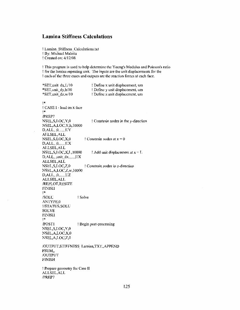
Lamina Stiffness Calculations

! Lamina_Stiffness_Calculations.txt ! By: Michael Maletta ! Created on: 4/12/08

! This program is used to help determine the Young's Modulus and Poisson's ratio ! for the lamina repeating unit. The inputs are the unit displacements for the ! each o f the three cases and outputs are the reaction forces at each face.

*SET,unit_dx,L/10 ! Define x unit displacement, um*SET,unit_dy,h/10 ! Define y unit displacement, um*SET,unit_dz,w/10 ! Define z unit displacement, um

!*! CASE I - load on x face !*/PREP7NSEL,S,LOC,Y,0 ! Constrain nodes in the y-directionNSEL,A,LOC,Y,h, 10000 D,ALL, , 0 , , , ,UY ALLSEL,ALLNSEL,S,LOC,X,0 ! Constrain nodes at x = 0D,ALL, , 0 , , , ,UX ALESEE, ALLNSEL,S,LOC,X,L,10000 ! Add unit displacement at x = LD,ALL, ,unit_dx,, , ,UXALLSEL,ALLNSEL,S,LOC,Z,0 ! Constrain nodes in z-directionNSEL,A,LOC,Z,w, 10000 D,ALL, , 0 , , , ,UZ ALLSELjALL /REPLOT,RESIZE FINISH !*/SOLU ! SolveANTYPE,0 !/STATUS,SOLU SOLVE FINISH !*/POSTl ! Begin post-processingNSEL,S,LOC,Y,0NSEL,A,LOC,X,0NSEL,A,LOC,Z,0

/OUTPUT,STIFFNESS_Lamina,TXT„APPENDFSUM,,/OUTPUTFINISH

! Prepare geometry for Case IIALLSEL,ALL/PREP7

125

DDELE,ALL,ALL


! Add unit displacement at y = d

! CASE II - load on y face !*NSEL,S,LOC,X,0 ! Constrain nodes in the x-directionNSEL,A,L0C,X,L, 10000 D,ALL, , 0 , , , ,UX ALESEE,ALLNSEL,S,LOC,Z,0 ! Constrain nodes in the z-directionNSEL,A,LOC,Z,w,10000 D,ALL, , 0 , , , ,UZ ALLSELjALL NSEL,S,LOC,Y,0 D,ALL, , 0 , , , ,UY ALLSEL,ALL NSEL,S,LOC,Y,h, 10000 D,ALL, ,unit_dy,, , ,UY ALLSEL,ALL /REPLOT,RESIZE FINISH !*/SOLU ANTYPE,0 !/STATUS,SOLU SOLVE FINISH !*/POSTlNSEL,S,LOC,Y,0 NSEL,A,LOC,X,0 NSEL,A,LOC,Z,0

! Solve


/OUTPUT,STIFFNESS_Lamina,TXT„APPEND FSUM,,/OUTPUTFINISH

! Prepare geometry for case III/PREP7ALLSEL,ALLDDELE,ALL,ALL

! CASE III - load on z face !*NSEL,S,LOC,Y,0 NSEL,A,LOC,Y,h, 10000 D,ALL, , 0 , , , ,UY A L L S E L ,A L L NSEL,S,LOC,X,0 NSEL,A,LOC,X,L, 10000 D,ALL, , 0 , , , ,UX ALLSEL,ALL NSEL,S,LOC,Z,0 D,ALL, , 0 , , , ,UZ ALLSEL,ALL NSEL,S,LOC,Z,w, 10000



! Constrain nodes at z = 0

! Add unit displacement at z = d

126

D,ALL, ,unit_dz,, , ,UZ ALLSEL,ALL /REPLOT,RESIZE FINISH !*/SOLU ! SolveANTYPE.O I/STATUS,SOLU SOLVE FINISH !*/POSTl ! Begin post-processingNSEL,S,LOG,Y,0NSEL,A,LOC,X,0NSEL,A,LOC,Z,0

/OUTPUT,STIFFNESS_Lamina,TXT„APPEND FSUM,,/OUTPUTFINISH

127

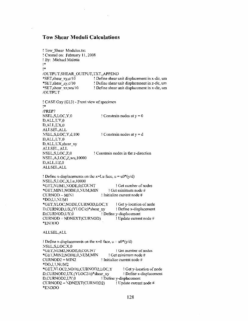
Tow Shear Moduli Calculations

! Tow_Shear_Modulus.txt ! Created on; February 11, 2008 ! By: Michael Maletta !*!*/OUTPUT,SHEAR_OUTPUT,TXT„APPEND*SET,shear_xy,c/10 ! Define shear unit displacement in x-dir, um*SET,shear_zy,c/10 ! Define shear unit displacement in z-dir, um*SET,shear_xz,wu/10 ! Define shear unit displacement in x-dir, um/OUTPUT

! CASE Gxy (G13) - Front view o f specimen !*/PREP7NSEL,S,LOG,Y,0 ! Constrain nodes at y = 0D,ALL,UY,0D,ALL,UX,0ALLSEL,ALLNSEL,S,LOC,Y,d, 100 ! Constrain nodes at y = dD,ALL,UY,0D,ALL,UX,shear_xyALESEE, ALLNSEL,S,LOC,Z,0 ! Constrain nodes in the z-directionNSEL,A,LOC,Z,wu, 10000 D,ALL,UZ,0 ALESEE, ALL

! Define x-displacements on the x=Lu face, u = uO*(y/d) NSEL,S,LOC,X,Lu, 10000*GET,NUM1 ,NODE,0,COUNT ! Get number o f nodes*GET,MIN 1 ,NODE,0,NUM,MIN ! Get minimum node #CURNOD = MINI ! Initialize current node #*D0,1,1,NUM1*GET,YLOC,NODE,CURNOD,LOC,Y ! Get y-location of nodeD,CURNOD,UX,(YLOC/c)*shear_xy ! Define x-displacementD,CURNOD,UY,0 ! Define y-displacementCURNOD = NDNEXT(CURNOD) ! Update current node #*ENDDO

ALESEE,ALL

! Define x-displacements on the x=0 face, u = uO*(y/d)NSEL,S,LOC,X,0* G E T ,N U M 2 ,N O D E ,0 ,C O U N T ! G e t n u m b e r o f n o d e s*GET,M1N2,NODE,0,NUM,M1N ! Get minimum node #CURN0D2 = MIN2 ! Initialize current node #*D0,J,1,NUM2*GET,YLOC2,NODE,CURNOD2,LOC,Y ! Get y-location o f nodeD,CURNOD2,UX,(YLOC2/c)*shear_xy ! Define x-displacementD,CURNOD2,UY,0 ! Define y-displacementCURN0D2 = NDNEXT(CURN0D2) ! Update current node #*ENDDO

128

! Solve

ALLSEL,ALL FINISH !*/SOLU ANTYPE,0 1/STATUS,SOLU SOLVE FINISH I*/POSTl NSEL,S,LOG,Y,c,10000 /OUTPUT,SHEAR_OUTPUT,TXT„APPEND FSUM,, ! Need sum in x-direction/OUTPUT ALLSEL,ALL

Begin post-processing

NSEL,S,LOC,X,Lu,IOOOO/OUTPUT,SHEAR_OUTPUT,TXT„APPENDFSUM,, ! Need sum in y-direction/OUTPUTALLSEL,ALLFINISH

! CASE Gzy (G23) - cross section o f specimen I*! Prepare geometry /PREP7DDELE,ALL,ALL!

I Apply Constraints NSEL,S,LOC,Y,0 D,ALL,UY,0 D,ALL,UZ,0 ALLSEL,ALL NSEL,S,LOC,Y,c,IOOOO D,ALL,UY,0 D,ALL,UZ,shear_zy ALLSEL, ALL NSEL,S,LOC,X,0 NSEL,A,LOC,X,Lu,IOOOO D,ALL,UX,0 ALLSEL,ALL


! Constrain nodes at y = d


! Define z-displacements on the z=wu face, w = wO*(y/d) NSEL,S,LOC,Z,wu, 10000 *GET,NUMI,NODE,0,COUNT * G E T ,M IN 1 ,N O D E ,0 ,N U M ,M IN CURNOD = MINI *DO,I,I,NUM I*GET,YLOC,NODE,CURNOD,LOC,Y D,CURNOD,UZ,(YLOC/c)*shear_zy D,CURNOD,UY,0 CURNOD = NDNEXT(CURNOD)♦ENDDO

! Get number o f nodes ! G e t m in im u m n o d e #I Initialize current node #

! Get y-Iocation o f node I Define z-displacement I Define y-displacement ! Update current node #

129

ALLSEL,ALL

! Define z-displacements on the z=0 face, w = wO*(y/d) NSEL,S,LOC,Z,0 *GET,NUM2,NODE,0,COUNT ♦GET,MIN2,NODE,0,NUM,MIN CURN0D2 = MIN2 ♦D0,J,1,NUM2♦GET,YLOC2,NODE,CURNOD2,LOC,Y D,CURNQD2,UZ,(YLGC2/e)^shear_zy D,CURNOD2,UY,0 CURN0D2 = NDNEXT(CURN0D2)♦ENDDO

! Get number o f nodes ! Get minimum node #! Initialize eurrent node #

! Get y-loeation o f node ! Define z-displaeement ! Define y-displacement ! Update eurrent node #

ALLSEL,ALLFINISH!♦/SOLUANTYPE,01/STATUS,SOLUSOLVEFINISHI*

! Solve

! Begin post-proeessing/POSTl NSEL,S,LOC,Y,c,IOOOO /OUTPUT,SHEAR_OUTPUT,TXT„APPEND FSUM,, I Need sum in z-direetion/OUTPUT ALLSEL,ALL

NSEL,S,LOC,Z,wu, 10000/OUTPUT,SHEAR_OUTPUT,TXT„APPENDFSUM,, I Need sum in y-direetion/OUTPUTALLSEL,ALLFINISH

! Prepare geometry for ease Gxz /PREP7 ALLSEL,ALL DDELE,ALL,ALL !

! CASE Gxz (G I2) - top faee o f specimen !♦I

NSEL,S,LOC,Z,0D,ALL,UX,0D ,A L L ,U Z ,0ALLSEL,ALLNSEL,S,LOC,Z,wu, 10000D,ALL,UZ,0D,ALL,UX,shear_xzALLSEL, ALLNSEL,S,LOC,Y,0NSEL,A,LOC,Y,c, 10000D,ALL,UY,0

I Constrain nodes at z = 0

I Constrain nodes at z = d

Constrain nodes in the y-direetion

130

ALLSEL,ALL

! Define x-displacements on the x=Lu face, u NSEL,S,LOC,X,Lu, 10000 *GET,NUM1,NODE,0,COUNT !♦GET,MIN 1 ,NODE,0,NUM,MIN !CURNOD = M INI !♦D0,I,I,NUM 1♦GET,ZLOC,NODE,CURNOD,LOC,Z D,CURNOD,UX,(ZLOC/wu)^shear_xz D,CURNOD,UZ,0 CURNOD = NDNEXT(CURNOD)♦ENDDO

= uO^(z/d)

Get number of nodes Get minimum node # Initialize current node #

Get z-location of node Define x-displacement Define z-displacement Update current node #

ALLSEL,ALL

! Define x-displacements on the x=0 face, u = uO^(z/d) NSEL,S,LOC,X,0 ♦GET,NUM2,NODE,0,COUNT ♦GET,MIN2,NODE,0,NUM,MIN CURN0D2 = MIN2 ♦D0,J,I,NUM 2♦GET,ZLOC2,NODE,CURNOD2,LOC,Z D,CURNOD2,UX,(ZLOC2/wu)^shear_xz D,CURNOD2,UZ,0 CURN0D2 = NDNEXT(CURN0D2)♦ENDDO

! Get number o f nodes ! Get minimum node #! Initialize current node #

! Get z-location o f node ! Define x-displacement ! Define z-displacement ! Update current node #

! Solve

ALLSEL,ALL FINISH !♦/SOLU ANTYPE,0 !/STATUS,SOLU SOLVE FINISH !♦/POSTl NSEL,S,LOC,Z,wu, 10000 /OUTPUT,SHEAR_OUTPUT,TXT„APPEND FSUM,, ! Need sum in x-direction/OUTPUT ALLSEL,ALL


NSEL,S,LOC,X,Lu, 10000/OUTPUT,SHEAR OUTPUT,TXT„APPENDFSUM,, ! Need sum in Z-direction/O U T P U TALLSEL,ALLFINISH

131

APPENDIX B: t-DISTRIBUTION TABLE [29]

fABlfi Bi M W nU Bim O N CRmCAl VAUiK

. TIBpnih#WHlyfdf a f AO I f A5 .#25 joa A1 ■DOS .(XB5 .001 .{«KW1 lAOO lATB 1.963 3.078 6314 1X71 ÜAP 31A2 63.66 1373 318X 636A

. 2 ,816 1.061 1.336 1.986 2.920 43CB 4A49 6365 1925 14.09 22X3 31A03 ,765 .978 1,250 1.638 2.353 3.182 1483 4J41 5,141 7.453 1021 1X924 .741 ,941 1.190 1.533 2.132 X776 XPPP 3.747 4.604 5398. 7.173 8.6103 .727 .3130 1,156 1.476 2MIS 2A71 XTfT 3Â6 4032 4.773 5.893 6A696 .718 A06 1.134 1.440 1.943 2447 X6U 3X43 3,707 4317, 5.208 55597 .711 AP6 1.119 1.415 1.895 X365 X517 1PP6 349P 4029 4785 5A088 ..706 A8P 1.108 1J97 1.8&) X306 M4P 2.896 1355 3.833 4X01 5M19 .703 A83 1.100 IJ ^ 1,833 2 ,m XfP# 2A21 3.250 3.690 4267 4781

10 .700 jm 1.093 1372 1,812 2228 X359 X764 116P 3581 4144 4X8711 .697 .876 1.088 1.363 1,796 X301 X328 1716 3,106 3AP7 4025 4.43712 .693 .873 1.083 1356 1.782 XÎ79 XfOf 1661 3.055 3A26 3,»0 4X1815 .870 1.079 1350 1.771 2.160 x m llffO 1012' 3J72 3.852 4.22114 j6M .868 1.076 1.345 1.761 X143 1264 2A24 1P7T 3326 3.787 4140If API ,866 1.074 1.341 1.753 2.131 IM P 2AQ2 1947 1366 3.733 407316 A90 .863 1.071 1337 1.746 X120 l à f 1563 1921 3X5X 3A86 401517 .689 .863 1.069 1,333 1.740 2.110 1224 1567 16P6 1222 3.646 3X651# A8* A63 1A57 1330 1.734 XlOl 1214 2A52 167* 3,197 3.611 3.9221* A # A61 1.066 1328 1.729 X0» 1206 153P 1661 3.174 3.579 3.88320 j«7 A60 t m 1,325 1.725 2.086 IIP? 1526 1645 3X53 3552 3.850a .686 A » 1,063 1.323 1.721 X080 H8P if ia 1631. 3.135 3527 3.81P22 .686 A38 1.061 1.321 1.717 2.074 1185 150» 1619 3.119 3505 3.7922) .685 8fS 1,060 1.319 1714 X069 2.177 1500 1607 3.104 3/485 37682* • .m A3f 1.059 1,318 1.711 X064 2À72 W 2 1797 3.»1 3467. 3.7452f .684 A * 1.058 1.316 1.708 2,060 1167 1465 2.787 3.078 3.450 3.725* .684 836 1.058 1315 1,706 X056 1162 147P 1779 . 3.067 3,435 3.70727 A84 A3f 1.037 1314 1.703 X0S2 1156 1473 2.771 3.057 3.421 3.690# . AA Aff t.OSÿ 1313 i.m X048 1154 1467 1763 3.047 3.408 3.6743» A88 AW 1.035 1.311 1J@P XM5 1150 1462 1756 3.038 3.396 3A5930 m A * 1.055 1.310 1AP7 X042 1147 2A37 2.750 3.030 3.385 3.64640 A81 A fl 1.030 1303 IA8* XOM 2,123 1423 1704 X971 3.307 3X5150 .679 .849 1.047 1399 1.676 X009 2.109 2.403 2.CT8 2.937 3.261 3.496<0 ATP A4# 1.045 lAPf XDOO lOPP 2J90 1660 2.915 3.232 3.46080 A78 .846 1.043 13» lAW lApQ lo w 1374 1639 2.887 3.195 3416

MO A?7 À43 1.042 lAW lA * 3A84 X061 1364 2A26 2A71 3.174 3X901000 A75 A42 I.W7 lAB 1A46 1Â62 2A56 1330 1561 X813 3.098 3X00

A74 A41 1.036 1382 1A45 1960 1034 1326 1576 2.807 3.091 3.291

do* 60* 70* #0* PO* 95# 96* 96* 99* PPA* 99.8# 99,9#

Cm&kmcelwdC

132

APPENDIX C: MISCALENEOUS DATA

Table C-1 : Square packed repeating unit o f tows inside a lamina mechanical properties.

Void Content % Ex (GPa) Ey (GPa) Ez (GPa) Vxy Vxz Vyx Vyz Vzx Vzy

0.00 99.05 6.12 6.66 0.333 0.323 0.021 0.404 0.022 0.4300.49 99.03 6,08 6.58 0.332 0.322 0.021 0.399 0.022 0.4220.30 98.83 6.09 6.44 0.332 0.322 0.021 0.404 0.022 0.4250.00 99.05 6.12 6.65 0.332 0.323 0.021 0.403 0.022 0.429

Table C-2: Hexagon packed repeating unit o f tows inside a lamina mechanical properties.

Void Content % Ex (GPa) Ey (GPa) Ez (GPa) Vxy Vxz Vyx Vyz Vzx Vzy

0.00 102.62 6.08 6.69 0.334 0.322 0.021 0.404 0.022 0.4390.11 102.61 6.04 6.61 0.334 0.322 0.021 0.404 0.022 0.439

Table C-3: The mechanical properties and constraints used for the three square packing configurationprogressive failure analyses.

Run Void Content (%)

Mechanical Properties Constraints

Ez (GPa) Vzx Vzy Srate_z (ttl) X o,z(m ) y o ,z (m )

No Voids 0.00 6.66 0.022 0.430 3.85E-06 -6.1 IE-09 -1.99E-07Center Void 0.49 6.58 0.022 0.422 3.85E-06 -6.02E-09 -1.95E-07Gap Voids 0.30 6.44 0.022 0.425 3.85E-06 -6.04E-09 -1.97E-07

Table C-4: The mechanical properties and constraints used for the two hexagon packing configurationprogressive failure analyses.

Run Void Content(%)

Mechanical Properties Constraints

Ez (GPa) Vzx Vzy rate z (tn) Xo,z(m) yo,z(m)

No Voids 0.00 6.69 0.022 0.439 4.23E-06 -9.02E-09 -3.70E-07Gap Voids 0.11 6.61 0.022 0.439 4.23E-06 -8.98E-09 -3.69E-07

133

Table C-5: The progressive failure results for the square packed tow repeating mit, first failed element

Square - No Voids Square - Center Voids Square - Gap Voids

Applied Gz F z ( N ) Oz (MPa)Initial

stiffness(MPa)

F z ( N ) Oz (MPa)Initial stiffness

(MPa) F z ( N ) Oz (MPa)Initial

stiffness(MPa)

0.003 0.330 19.84 18.49 0.326 19.60 18.27 0.327 19.62 17.900.006 0.659 39.55 36.97 0.651 39.07 36.54 0.652 39.12 35.800.008 0.985 59.15 55.46 0.973 58.42 54.81 0.974 58.46 53.700.011 1.296 77.81 73.95 1.271 76.33 73.07 1.264 75.91 71.590.014 1.569 94.22 92.44 1.460 87.64 91.340.017 1.650 99.07 110.92

Table C-6: The progressive failure results for the hexagon packed tow repeating unit,/j/-sf fa iled element

Hexagon - No Voids Hexagon - Gap Voids

Applied Gz F z ( N ) Oz (MPa)Initial

stiffness(MPa)

F z ( N ) Oz (MPa)Initial

stiffness(MPa)

0.003 0.904 19.87 18.58 0.600 19.79 18.580.006 1.802 39.62 37.16 1.197 39.46 37.160.008 2.695 59.25 55.74 1.789 59.02 55.740.011 3.582 78.76 74.32 2.378 78.44 74.320.014 4.435 97.52 92.90 2.943 97.07 92.900.017 5.174 113.76 111.48 3.432 113.18 111.480.019 5.635 123.90 130.06

134

the development of a progressive failure model of a fiber

Documents