the development of a power system simulator using …
TRANSCRIPT

THE DEVELOPMENT OF A POWER SYSTEM SIMULATORUSING MULTIPLE MICROPROCESSORS
by
RAYMOND BRIAN ISHMAEL JOHNSON MA
Thesis submitted for the degree of Doctor of Philosophy
in the Faculty of Engineering
Department of Electrical Engineering Imperial College of Science and Technology
University of London
London, December 1984
2
ABSTRACT
Recent advances in micro-electronics have motivated several proposals to implement power system simulators based on multiple microprocessors executing in parallel. This thesis details the hardware and software development of such a simulator for operator training and research.
The Project utilises off-the-shelf equipment and thus hardware development is limited to devising a suitable interconnection strategy to realise a parallel processing architecture. The resulting multiple processor network is controlled by a host minicomputer.
A distributed monitor is developed for interprocessor communication and synchronisation. Its flexibility is demonstrated by using its primitive operations to construct other high-level protocols. Time-dependent errors such as deadlock and lockout are identified and guidelines given on their avoidance.
A model of interactive computation is developed for the design of the man/machine interface. Based on role models of the part man plays in interactive systems, it provides a framework for designing consistent user interfaces. This is used to implement a versatile control program.
A short/mid-term power system dynamic simulation is formulated vith detailed models of generating plant and loads. Problem partitioning for solution on the multiple processors is achieved by assigning the equations representing individual components to separate processors.
The scope of this thesis includes the solution of the set of non-linear algebraic and differential equations which describe the system dynamics. The numerical problems in time integration such as the treatment of discontinuities, control of round-off and truncation errors, and numerical stability are fully discussed and various new approaches are investigated. An integration method which can be numerically tuned to

suit the system of equations is developed and it is shown to be superior to the trapezoidal rule when very long time-steps are used.
A comprehensive simulation environment has been implemented to set up, run and control interactive power system simulations. The performance of the simulator is assessed and examples are given of the types of studies that may be conducted. The implications of the results are discussed and proposals are made for the future expansion of the simulator.

- 4 -
Liandikwalo halifutiki

- 5 -
ACKNOWLEDGMENTS
The work presented in this thesis was carried out under the supervision of Dr. M.J. Short, B.Sc., Ph.D, D.I.C., C.Eng., M.I.E.E., M.I.E.E.E., whom the author thanks for his help and advice.
I express my sincere appreciation to Dr. B.J. Cory, D.Sc.(Eng.), A.C.G.I., C.Eng., F.I.E.E., Sen.M.I.E.E.E., Reader in Electrical Engineering, for his interest and constant encouragement. The successful completion of this research owes a great deal to him.
The project was funded by the Science and Engineering Research Council under Research grant No. GR/B/1626.9* I am grateful to them for providing me with financial support in the form of a Research studentship.
The other members of the simulator project, Raphael Lopez and Isaias Elizarraraz, deserve special mention for their friendship and their willingness to discuss new ideas. As friendly users, they ensured the user-friendliness of the interactive program.
My colleagues in the Power Systems Section and friends in and out of College have contributed in many different ways to the successful completion of this work. In particular, I thank my brother Ronald and his family who were very supportive throughout the period of this research.

TABLE OF CONTENTS
Page
ABSTRACT 2
ACKNOWLEDGEMENTS 5
LIST OF FIGURES 12
LIST OF TABLES - 14
LIST OF SYMBOLS AND ABBREVIATIONS 15
CHAPTER 1 : INTRODUCTION
1.1 GENERAL 18
1.2 PARALLEL PROCESSING HARDWARE AND SOFTWARE 191.2.1 Parallel computer architectures 191.2.2 Software for parallel processing 231.2.3 Interprocess communication and synchronisation 23
1.3 SIMULATION OF POWER SYSTEM DYNAMICS 251-3-1 Simulation techniques 251.3*2 Partitioning methods 261.3*3 Interactive computing 27
1.4 PROJECT OVERVIEW AND SCOPE OF WORK 271.4*1 Objectives 271.4*2 Project description 28
1.5 THESIS ORGANISATION 29
CHAPTER 2 : HARDWARE STRUCTURE
2.1 INTRODUCTION 31

7
2.2 THE MICROPROCESSOR UNITS 312.2.1 The Texas TMS 9900 microprocessor 332.2.2 Input/output ports and controllers 34
2.3 HOST MINICOMPUTER AND PERIPHERALS 352.3*1 The host minicomputer and development system 352.3*2 Peripherals and ancillary devices 362.3*3 The programmable electronic switch 36
2.4 THE MULTIPLE PROCESSOR SYSTEM 382.4*1 The multiple processor architecture 382.4*2 Mechanisms for interprocessor communication 412.4*3 Interprocessor communication 42
2.5 AN ARCHITECTURE FOR LARGE SYSTEMS 44
2.6 CONCLUDING REMARKS 46
CHAPTER 3 : SOFTWARE FOR PARALLEL PROCESSING
3*1 INTRODUCTION 47
3*2 PROGRAMMING LANGUAGES 483*2.1 Pascal language structure 483*2.2 Features of Texas Instruments Microprocessor Pascal 483*2.3 Other programming languages 503.2.4 Software development process 51
3.3 COMMUNICATION BETWEEN COOPERATING PROCESSORS 533*3*1 Structuring concepts in parallel processing 533*3*2 Synchronisation and communication mechanisms 54
3*4 DISTRIBUTED MONITORS FOR INTERPROCESSOR COMMUNICATION 543.4.1 Structure 543*4*2 Implementation 563*4*3 Message-passing primitives 593.4.4 Higher level communication protocols 62

b
5-5 PROGRAMMING FOR PARALLEL EXECUTION5*5*1 Factors causing loss in performance 5*5.2 Time-dependent errors
5.6 ANALYSIS OF A PARALLEL ALGORITHM5.6.1 Problem description5.6.2 Some performance measures5.6.5 Analysis of computation patterns5.6.4 Implications for large systems
5.7 CONCLUSIONS
CHAPTER 4 : INTERACTIVE COMPUTATION
4.1 INTRODUCTION
4.2 MAN/MACHINE AND MACHINE/MACHINE INTERFACES4.2.1 Models of human behaviour4.2.2 Interaction patterns4.2.5 Dialogue types4.2.4 A model of interactive computation4.2.5 Input/output and communication
4.5 DESCRIPTION OF THE INTERACTIVE PROGRAM
4.4 DESCRIPTION OF COMMANDS4.4.1 Command structure4.4.2 Control and initialisation commands4.4.5 Utility commands4.4.4 Interactive commands
4.5 'PROGRAMMING AND RUNNING INTERACTIVE SIMULATIONS4.5.1 Interfacing simulation programs for interaction4.5.2 Programming command files4.5.5 Programming display files4.5.4 Operation of the interactive control program
4.6
656567
6869697174
74
77
787878818185
84
85858588
89
9090959596
CONCLUSIONS 97

- 9 -
CHAPTER 5 : POWER SYSTEM MODELS AND SIMULATION TECHNIQUES
5.1 INTRODUCTION 98
5.2 THE INTERCONNECTING NETWORK 995.2.1 Network models for stability analysis 995.2.2 Data preparation 1005.2.3 Network solution 100
5-3 GENERATION PLANT MODELS 1015*3«1 The synchronous generator 1015-3*2 Excitation subsystem 1035.3*3 Speed governor and turbine models 106
5*4 LOAD REPRESENTATION 1065*4*1 Static load representation 1085*4*2 Dynamic load representation 1095*4*3 Composite bus loads 111
5.5 FORMULATION OF THE COMPOSITE SYSTEM MODEL 1125*5*1 The composite generation plant model 1125*5*2 Interfacing dynamic components to the network 112
5.6 NUMERICAL INTEGRATION METHODS 1145*6.1 Characterisation of integration methods 1145*6.2 Explicit methods 1155.6.3 Implicit methods 1165.6.4 State transition matrix 118
5.7 TUNABLE NUMERICAL INTEGRATION 1195.7*1 Comparison with classical methods 1195.7.2 Round-off and truncation errors 1205.7.3 Stability properties 1255.7.4 Trajectory errors 126
5.8 CONCLUDING REMARKS 129
CHAPTER 6 : IMPROVED TECHNIQUES FOR DYNAMIC SIMULATION
6.1 INTRODUCTION 132

10
6.2 SIMULATION ALGORITHM 1356.2.1 Partitioned solutions 1356.2.2 Solution of the swing equations 1356.2.5 Simulation of a generator and its controls 1386.2.4 Convergence criteria 1396.2.5 Solution algorithm 139
6.3 TREATMENT OF NONLINEARITIES 1456.3*1 Discontinuities 1456.3*2 Solution of trigonometric functions 1486.3*3 Solution of the load equations 148
6.4 APPLICATION OF TUNABLE INTEGRATION 1506.4*1 Derivation of difference equations 1506.4*2 Tuning strategies 1516.4*3 Fixed tuning methods 1516.4*4 Adaptive tuning methods 1526.4*5 Evaluation of the method 155
6.5 POWER SYSTEM STABILITY 161
6.6 CONCLUSIONS 163
CHAPTER 7 : INTERACTIVE DYNAMIC SIMULATION
7.1 INTRODUCTION 164
7.2 DESCRIPTION OF THE SIMULATION PROGRAM . 1647.2.1 Program structure 1647.2.2 Partitioned algorithm 1667*2.3 Interprocessor communication 169
7.2.4 Interface to the interactive control program 169
7.3 PERFORMANCE TESTS 1707*3*1 Test systems 1707*3*2 Sequential algorithm 1707.3*3 Parallel algorithm 172

7 . 4 INTERACTIVE FEATURES 1747.4.1 Simulation set-up and control 1747.4.2 Network switching and load changes 1747.4.3 Interaction with generators and motors 1757.4.4 User interaction 1757.4.5 Post-processing 177
7 . 5 SIMULATION STUDIES 1777.5.1 Critical fault clearing time 1777.5.2 Pole slipping and resynchronisation 1787.5.3 Non-impedance load representation 178
7 . 6 CONCLUSIONS 178
CHAPTER 8 : CONCLUSIONS
8.1 GENERAL 183
8.2 HARDWARE AND SOFTWARE 1838.2.1 Hardware 1838.2.2 Software 1848.2.3 Interaction 185
8.3 SIMULATION TECHNIQUES 1868.3.1 Model formulation 1868.3.2 Solution methods 1868.3.3 Parallel algorithms 187
8 . 4 ORIGINAL CONTRIBUTIONS 187
8.5 SUGGESTIONS FOR FURTHER WORK 1888.5.1 Model reduction 1888.5.2 Simulator expansion 1898.5.3 Simulator applications 190
APPENDIX A : TIMP IMPLEMENTATION BENCHMARKS APPENDIX B : TEST SYSTEMS DATA REFERENCES
191193199

12
Fig. 1.1 Anderson and Jensen’s taxonomy. 21Fig. 1.2 Typical system topologies. 22Fig. 1.3 Synchronisation techniques and language classes. 24Fig. 2.1 MPU functional block diagram and memory map. 32Fig. 2.2 Schematic diagram of electronic switch. 37Fig. 2.3 Multiple MPU simulator : Hardware configuration. 39Fig. 2.4 Architectural configurations. 40Fig. 2.5 MPU-MPU interconnection and timing diagram. 43Fig. 2.6 Proposed multiple processor architecture. 45Fig. 3*1 TIMP Pascal system structure. 49Fig. 3*2 Software development process. 52Fig. 3*3 Hierachical structure of the distributed monitor. 57Fig. 3*4 Interprocessor communication data-flow schematic. 58Fig. 3»5 Port and message buffer data structures. 56Fig. 3*6 Implementation of the distributed monitor. 60Fig. 3*7 Implementation and decomposition penalties. 66Fig. 3*8 Types of deadlock. 68Fig. 3*9 Typical computation patterns. 70Fig. 3*10 Effect on computation pattern of communication schemes. 72 Fig. 3*11 Performance curves for single-stage computation. 73Fig. 3*12 Performance curves for. double-stage computation. 75Fig. 4*1 Data flows in Man/Machine interaction. 80Fig. 4.2 Hierarchical model of interactive computation. 82Fig. 4*3 Structure of the interactive control program. 86Fig. 4.4 Command tree. 87Fig. 4*5 Host/Multiple-MPU communication scheme. 91Fig. 4.6 Example of a command file. 94Fig. 4*7 Example of a display file. 95Fig. 5*1 Generation plant model. 102Fig. 5«2 Generator equivalent circuit and block diagram. 104Fig. 5*3 Excitation subsystem model. 105Fig. 5*4 Governor-Turbine model. 107Fig. 5*5 Static and dynamic load models. 110Fig. 5*6 Generation plant model matrix. 113Fig. 5*7 Stability boundaries of conventional integration methods. 117Fig. 5*8 Variation of tuning parameter with h^. 121Fig. 5*9 Behaviour of global error. 123
LIST OF FIGURES

Fig. 5*10 Variation of truncation error with tuning parameter. 124Fig. 5*11 Stability boundaries of tunable integration method. 127Fig. 5*12 Trajectory error diagrams of conventional methods. 128Fig. 5*13 Trajectory error diagrams of tunable methods. 130Fig. 6.1 The WSCC 9-Bus test system. 134Fig. 6.2 Comparison of solution methods for the swing equations* 137Fig. 6.3 Variation of iterations with convergence tolerance. 140Fig. 6.4 Effect of convergence tolerance on time response. 141Fig. 6.5 The effect of step length on time response : Faulted case. 143Fig. 6.6 The effect of step length on time response : Outage case. 144Fig. 6.7 Treatment of discontinuities. 147Fig. 6.8 Approximate sines and cosines. 149Fig. 6.9 Fixed global tuning. 153Fig. 6.10 Variation of iterations with the tuning parameter. 154Fig. 6.11 Behaviour of tuning parameters of Governor-Turbine states. 156 Fig. 6.12 The effect of step length on time response :
A-stable tuning. 158Fig. 6.13 The effect of step length on time response :
Full tuning. 159Fig. 6.14 Comparative plots of tuned methods and trapezoidal rule. 160 Fig. 6.15 Solution accuracy of marginally stable and unstable cases. 162 Fig. 7»1 Power system simulator : software structure. 165Fig. 7.2 Typical Pascal data structures. 157
Fig. 7.3 Serial and parallel simulation algorithms. ̂53
Fig. 7.4 IEEE 14-bus and 30-bus test systems. 171Fig. 7.5 Parallel simulation timing diagrams. 173Fig. 7.6 Typical simulator display pages. 176Fig. 7.7 Marginally stable cases. 179Fig. 7.8 Pole-slipping and resynchronisation. 180Fig. 7.9 The effect of load representation. 181
- 13 -

14
LIST OF TABLES
Table 2.1 Comparison of TMS 9900 with other commercialmicroprocessors. 33
Table 3*1 Communication and synchronisation primitives. 55Table 4.1 Sequence of interactive computation. 79Table 4*2 Man/machine dialogue types. 81Table 4*3 Interactive system design parameters. 82Table 4«4 Overhead due to communication. 93Table 4«5 List of symbols used in display files. 94
Table 4*6 List of symbols used in command files. 94Table 5*1 Single-step integration methods. 120Table 6.1 Simulating difference equations for the swing equations. 136Table 6.2 Effect of time-step on the number of iterations. 142Table 6.3 Simulation program timings. 157Table 6.4 Number of iterations per step of TR and tunable methods. 157Table 7.1 Sequential algorithm program timings. 170Table 7.2 Parallel algorithm program timings. 172Table A.1 Execution speed of Texas Pascal constructs. 191Table A.2 Execution speed of floating-point arithmetic'. 192Table B.1 WSCC 9-bus system : network data. 193Table B.2 WSCC 9-bus system : base case loadflow solution. 193Table B.3 IEEE 14-bus system : network data. 194Table B.4 IEEE 14-bus system : base case loadflow solution. 194Table B.5 IEEE 30-bus system : network data. 195Table B.6 IEEE 30-bus system : base case loadflow solution. 196
Table B.7 Rotating machine data. 197Table B.8 Exciter data. 197Table B.9 Power system stabiliser data. 198Table B.10 Governor-turbine data. 198

15
LIST OF SYMBOLS AND ABBREVIATIONS
In general, symbols and abbreviations are defined the first time they appear in the text.
PRINCIPAL SYMBOLS[A]d,qD_f,gF, GhHIm,Re[ i ]
V 1,3 = V -1
nNpco
pvp
P' = dP/dVPPomQqo>qv
RaS = P+jQ t = nh Tm ' rp »ido* iqom" m*'^o* qom" ,TI f
q
Linear system matrix Direct and quadrature axes Turbine damping coefficient Vector functions Numerical integration factors Integration step length Generator inertiaImaginary and real parts of a complex numberVector of bus currentsd and q components of terminal currentImaginary operatorIntegration step countNumber of microprocessor unitsActive load frequency regulation coefficientActive load voltage regulation coefficientBus active powerAcceleration powerElectrical powerDifferential of power with respect to voltage Initial steady-state load active power Mechanical power Bus reactive powerReactive load frequency regulation coefficientReactive load voltage regulation coefficientStator resistanceComplex powerTime instantTime constantD and q-axes open circuit transient time constants D and q-axes open circuit subtransient time constants D and q-axes short circuit subtransient time constants
16
[T][U][V]Vcrit V = 1 -w
W VdqV V Vir
Xd ’XqXd
Y "AdY"Xqx,y
XH ,XLYoM b u s^ b u sAx5X
7 = D/2H </>= 1/2H
^ref cu = ft
rWrt
ref
Transformation matrixUpper triangular matrixVector of bus voltagesMotor load stalling voltageComplement of tuning parameterd and q components of voltageImaginary and real components of voltageTuning parameterSynchronous reactancesD-axis transient reactanceQ-axis transient reactanceD-axis subtransient reactanceQ-axis subtransient reactanceState variablesHigh and low limits on variable xNorton equivalent shunt admittanceAdmittance matrixImpedance matrixIncrement in xRotor electrical angleEigenvalue or rootDamping/inertia ratioinverse of inertiaRotor angular speed, synchronous speed Rotor angular speed deviation Damping ratio Natural frequency
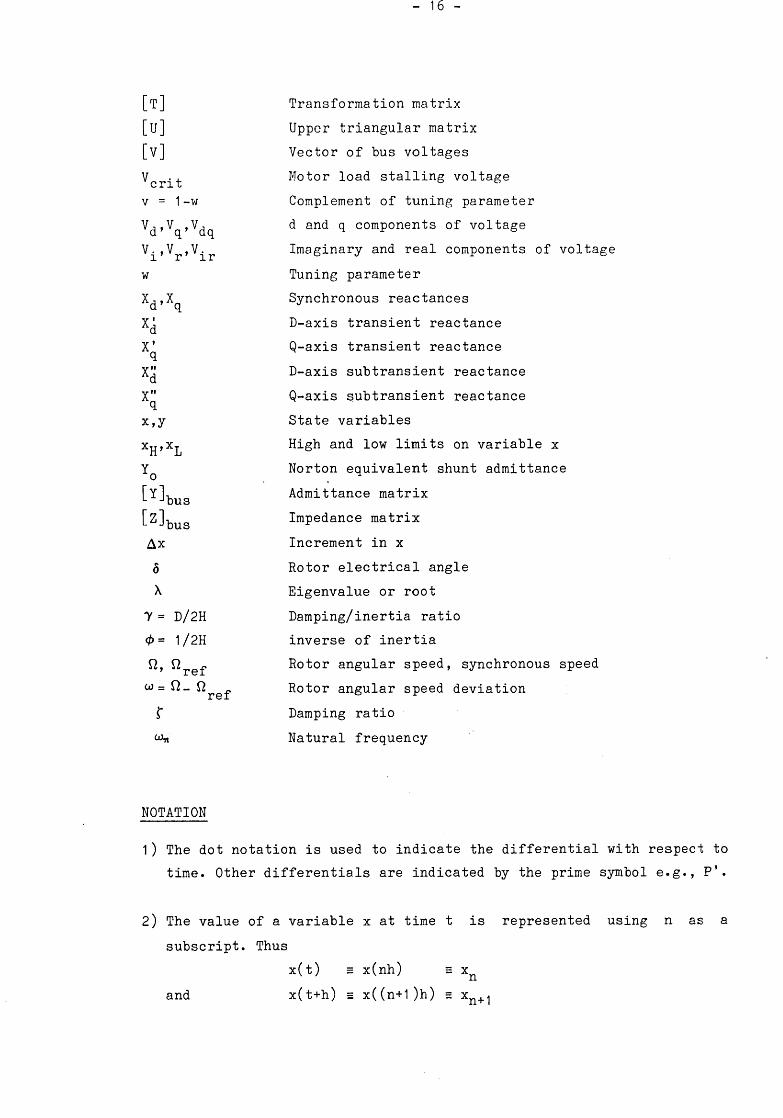
NOTATION
1) The dot notation is used to indicate the differential with respect to time. Other differentials are indicated by the prime symbol e.g., P'.
2) The value of a variable x at time t is represented using n as a subscript. Thus
x(t) = x(nh) = xnx(t+h) s x((n+l)h) s xn+1and
17 -
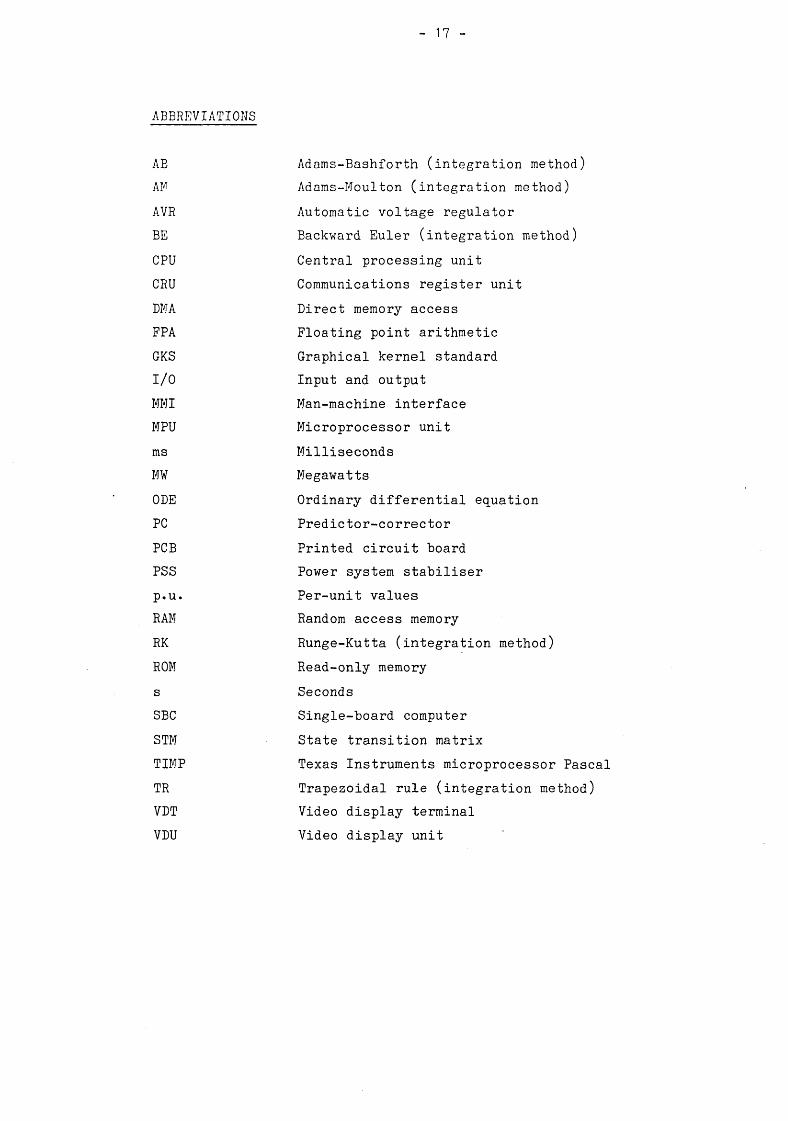
ABBREVIATIONS
AE Adams-Bashforth (integration method)AN Adams-Moulton (integration method)AVR Automatic voltage regulatorBE Backward Euler (integration method)CPU Central processing unitCRU Communications register unitDMA Direct memory accessFPA Floating point arithmeticGKS Graphical kernel standardI/O Input and outputMM I Man-machine interfaceMPU Microprocessor unitms MillisecondsMW MegawattsODE Ordinary differential equationPC Predictor-correctorPCB Printed circuit boardPSS Power system stabiliserp.u. Per-unit valuesRAM Random access memoryRK Runge-Kutta (integration method)ROM Read-only memorys SecondsSBC Single-board computerSTM State transition matrixTIMP Texas Instruments microprocessor PascalTR Trapezoidal rule (integration method)VDT Video display terminalVDU Video display unit
18
CHAPTER 1
INTRODUCTION
1.1 GENERAL
Computation machinery for power systems analysis and simulation has progressed from the early AC network analysers, through analogue computers to digital computers. Larger problem sizes plus the increasing requirement for real-time simulation and on-line control has prompted researchers in power systems to investigate the feasibility of using various combinations of hardware operating in parallel to obtain high-speed solutions.
This effort started in the 1960s and various hybrid machines were constructed utilising combinations of network analysers, analogue and digital computers. One such system was constructed at Imperial College and used successfully for real-time control studies (Arriola-Valdes and others [l], Mogridge and others [2]). Michaels [3] has demonstrated the
possibility of obtaining load flow and transient stability solutions 100 times faster than real-time. While these efforts confirmed the power of the approach, the high cost of the equipment, its intrinsic lack of flexibility and its physical size has discouraged its general acceptance by the industry.
The favourable price/performance of digital computer hardware led to proposals for multicomputer networks for general simulation by Korn [4], and for power system computation by Happ [5]. The invention of the microprocessor and its subsequent rapid development and falling cost are now regarded as a most promising avenue towards achieving high-speed scientific computation. Thus several researchers in the field of simulation in general and power systems in particular have proposed structures of multiple micro-processing units (MPUs) on which

19 -
computations may be carried out in parallel [6-11].
Early proposals (e.g. Ref. [6]) envisaged large numbers of processors interconnected in a regular pattern being capable of execution speeds of millions of floating-point operations per second (MFLOPs) with a substantial cost advantage over supercomputers. It is now recognised that the irregular nature of most computing tasks and architectural problems such as resource contention, would result in saturation which would limit the maximum number of processors that can be used effectively. Therefore, present research concentrates on achieving a more modest speed-up for large problems partitioned over relatively few processors, say 40-50 [8—11]-
1.2 PARALLEL PROCESSING HARDWARE AND SOFTWARE
1.2.1 Parallel computer architectures
The desire for fast computing at minimum cost has been the primary motivation behind the increasing use of parallel computing systems. Parallelism has been exploited "in the small" by carrying out task decomposition at the computer cycle or instruction level and this has given rise to architectures such as those of vector supercomputers, pipelined computers and array processors ([12-14])*
Parallel computer systems which exploit parallelism in the small can be characterised by the taxonomy proposed by Flynn in 1966 [12] where the possible types of computer architectures are defined in terms of the parallelism or otherwise of the instruction and data streams. In Flynn's taxonomy there are thus four possible types of computers, namely:
SISD - single instruction stream, single data stream.This is the classification of the prevalent von Neumann architecture where instructions and data reside in a single memory space.
20
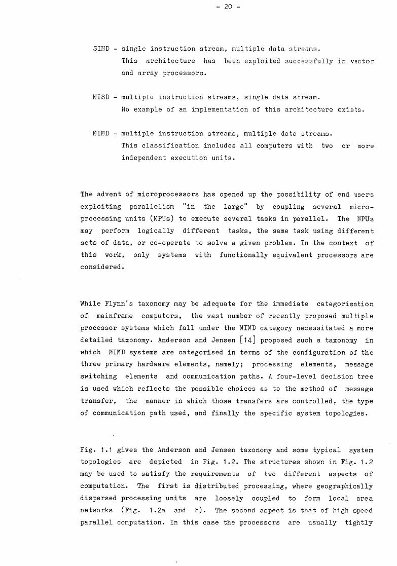
SIND - single instruction stream, multiple data streams.This architecture has been exploited successfully in vector and array processors.
MISD - multiple instruction streams, single data stream.No example of an implementation of this architecture exists.
MIMD - multiple instruction streams, multiple data streams.This classification includes all computers with two or more independent execution units.
The advent of microprocessors has opened up the possibility of end users exploiting parallelism "in the large" by coupling several microprocessing units (MPUs) to execute several tasks in parallel. The MPUs may perform logically different tasks, the same task using different sets of data, or co-operate to solve a given problem. In the context of this work, only systems with functionally equivalent processors are considered.
While Flynn's taxonomy may be adequate for the immediate categorisation of mainframe computers, the vast number of recently proposed multiple processor systems which fall under the MIMD category necessitated a more detailed taxonomy. Anderson and Jensen [14] proposed such a taxonomy in which MIMD systems are categorised in terms of the configuration of the three primary hardware elements, namely; processing elements, message switching elements and communication paths. A four-level decision tree is used which reflects the possible choices as to the method of message transfer, the manner in which those transfers are controlled, the type of communication path used, and finally the specific system topologies.
Fig. 1.1 gives the Anderson and Jensen taxonomy and some typical system topologies are depicted in Fig. 1.2. The structures shown in Fig. 1.2 may be used to satisfy the requirements of two different aspects of computation. The first is distributed processing, where geographically dispersed processing units are loosely coupled to form local area networks (Fig. 1.2a and b). The second aspect is that of high speed parallel computation. In this case the processors are usually tightly

TRANSFERSTRATEGY
TRANSFERCONTROLMETHOD
TRANSFERPATHSTRUCTURE
DEDICATEDPATH
l^ t
DIR LCT
(NONE)
JL
SYSTEMARCHITECTURE
(DDL)LOOP
(DDC)COMPLETE
INTERCONNECTION
INTERCONNECTION FOR COMMUNICATION
CENTRALIZEDROUTING
SHAREDPATH
DEDICATEDPATH
SHAREDPATH
r = \(DSM) (DSB) (ICDS) (ICDL) (ICS)
CENTRAL GLOBAL STAR LOOP BUSMEMORY BUS WITH WITH
CENTRAL CENTRAL _________ SWITCH SWITCH
INDIRECT_i i__
DECENTRALIZEDROUTING
__ U \____
DEDICATED SHAREDPATH PATH
(IDDR) MODI) (IDS)REGULAR IRREGULAR BUSNETWORK NETWORK WINDOW
iroi
Fig. 1.1 Anderson and Jensen's taxonomy

22
LOOP COMPLETE
a) DDL (loop) b) DDC (complete interconnection)
OIRECT INDIRECT
DEDICATED SHARED
/ \MEMORY BUS
c) DSM (multiprocessor) d) DSB (global bus)
e) DSB (global bus with dual-ported memory)
Fig. 1.2 Typical system topologies.
23 -
coupled via a parallel bus on a common backplane.
Parallel bus systems are commonly available in one of two forms. Ore is the DSM scheme (Fig. 1.2c) where a large global memory is used to facilitate inter-processor communication and to store data common to all MPUs. In another more flexible scheme, each MPU has a dual-ported memory through which messages may be sent and received from other processors (see Fig. 1.2d and e). In both schemes exclusive access to the system bus is granted in turn to each processor on a priority basis when interprocessor communication is required.
1.2.2 Software for parallel processing
The predominant language used in scientific computation is Fortran -which was originally designed specifically for this purpose. However, its small number of control structures and restricted set of data types make it an inefficient language in which to write large reliable programs.
Pascal (see Jensen and Wirth [16]), a language based on the concept of structured programming, has a wide variety of data structures and a flexible set of control constructs. Enns et al. [17] recommended its use as an alternative language for power system computations. In its concurrent form, Pascal is well suited to the application of parallel processing (Brinch Hansen [18]). An alternative is ADA (USDOD [19])» which may be regarded as a superset of PASCAL.
1.2.3 Interprocess communication and synchronisation
In the development of concurrent, multi-tasking operating systems, several programming constructs have been defined which allow synchronisation and message passing between different tasks [18-23]- The advent of parallel systems comprising several processors has resulted in efforts to exploit this acquired knowledge.

- 24 -
In a recent survey paper [23], Andrews and Schneider traced the development of the various software tools available up to the present state-of-the-art. Fig. 1.3 indicates the two main development paths followed, up to the development of the remote procedure call which is the technique used in ADA [ 19]* A H concurrent languages are viewed as belonging to one of three classes: procedure oriented, message oriented or operation oriented. Procedure oriented languages (e.g. Brinch Hansen’s Concurrent Pascal [ 1 s]) are usually based on the monitor [21 ] and they are most suitable for serial processors although they can be implemented on multiprocessors as well. Message oriented languages, such as Hoare's CSP [22], are better suited to multiple processor systems without common memory. Operation oriented languages (e.g. ADA) are the most versatile since they combine the advantages of the other two classes.
A multiprocessor system may be programmed as a concurrent system with several tasks distributed over the various processors of the system. In true multiprocessors, the operating systems are either centralised or distributed with common data stored in global memory (Enslow [13]* Jones and Schwarz [24]). In multiple processor systems without common memory a distributed operating system is necessary (see Halsall et al. [25]).
PROCEDUREORIENTED
Busy-WaitingI
Critical Regions
/Monitors
Semaphores
MESSAGEORIENTED
Message Passing
Path Expressions \
Remote Procedure Call
OPERATION ORIENTED
Fig. 1.3 Synchronisation techniques and language classes.

25 -
1.3 SIMULATION OF POWER SYSTEM DYNAMICS
1-3-1 Simulation techniques
The computations required in power system analysis and design are such that the need for economic computing power has never been fully satisfied. Although the execution speed and memory capacity of computers have been increasing rapidly in recent years, increases in the size and complexity of power systems over the same period have resulted in vastly increased computational requirements.
Efforts to improve the execution speeds of such large problems have been made by one of three complementary approaches. The first is that of model reduction or simplification [26-28]. In dynamic stability studies simplified generator models are used; Hammons and others [26] and Alden and Nolan [27] have investigated the effect of modelling detail on the accuracy of simulation studies. Another method of reduction is the derivation of equivalents for groups of generators that are known to "be coherent (Ghafurian and Berg [28]).
A second approach involves research into better solution methods and new numerical algorithms. Examples include the development of stiffly- stable multi-step integration methods (Gear [29], Fuller et al. [30]) and the application of implicit integration methods to the transient stability problem (Dommel and Sato [3 1]). Major improvements in the solution of the network algebraic equations resulted from the use of sparsity techniques by Tinney and Walker [32] and the development of the fast decoupled load flow (FDLF) by Stott and Alsac [33]*
The third approach is that of exploiting new computer architectures in order to achieve speed gains. Orem and Tinney investigated the potential of array processors in solving large-scale power system problems [34] and the Electric Power Research Institute in the USA (EPRl) has funded research into the use of vector computers (Happ [35])- The major part of this effort was devoted to the derivation of parallel solution

26
algorithms and various matrix forms were developed which improved the performance of these types of architectures. However, the viability of these efforts has been recently called into question (Detig [36]). Proposals to use several independent processors in a multiple processor configuration now seem to be more promising [9—11].
1.3-2 Partitioning methods
The primary direction of research into parallel processing by power systems analysts has been towards efficient methods of partitioning power systems problems for parallel execution. It is well known that this aspect is heavily dependent on the architecture of the hardware on which the problem is to be solved. Various methods have been put forward to handle the large set of algebraic and differential equations describing power system simulation problems.
Mathematical approaches to partitioning have been proposed which require the differential equations to be discretised such that they can be solved together with the network equations [9—11]- The resulting set of equations can then be ordered into a convenient form and partitioned for solution on several MPUs. One disadvantage of such techniques is that it is usually difficult to identify which equations represent the various components of the physical system. Also, during solution, frequent exchanges of large amounts of data between the processors are required although this may be minimised by the use of clustering techniques (Fong and Pottle [ 1 1 ] ).
A more straightforward method of decomposition is to partition the system of equations into sets that represent physically identifiable components of the power system (Fong and Pottle [11]). This has the advantage that the equations of individual components can be solved on separate processors. Also, if generators and motors are regarded as components of the power system, the differential equations are separated from the algebraic equations and appropriate solution algorithms may be used for each part.

1.3-3 Interactive computing
An important concern in the development of a simulator, whether for training, research or design, is the level of user-interaction to be incorporated [38,39]- Since simulation activities in general require multiple runs of programs with different data, the interactive facilities must be designed such that changes can be made with the minimum of effort. In the present context, the definition of Undrill and colleagues [39] is adopted viz.
"An interactive program is one that allows the engineer to exercise his ability to make decisions in the course of the run to influence its future progress".
Such decisions may range from simply halting the program to control actions aiming to stabilise the system being studied.
1.4 PROJECT OVERVIEW AND SCOPE OF WORK
1.4*1 Objectives
A project was initiated in 1979 by Short and Cory at Imperial College to investigate the applicability of the new 16-bit microprocessors to the simulation of power- systems dynamics by parallel processing [40]. The three main objectives of project may be stated as follows:
1. To determine the potential of microprocessors as the basic elements in a dynamic power system simulator for the fast solution of power system dynamic and operating problems.
2. To construct a flexible, expandable multi-machine power system simulator composed of an array of microprocessors.
3. To establish an optimum simulator architecture and software structure for power system investigations.

1.4-2 Project description
In line with the original project proposals, commercially available single-board computers and a host minicomputer system were used. This reduced the development time in that a minimum of special-purpose hardwa-re had to be built. In anticipation of the future predominance and widespread use of structured languages, Pascal was chosen as the main programming language to be used in the research project. This also ensured portability of the simulation programs.
The work presented in this thesis was carried out as part of the simulation project which was undertaken by three workers including this author. The aspects covered by the author's colleagues are indicated in the following:
Elizarraraz [41] investigated network solution algorithms .for load flow studies and fault analysis using -dynamic data structures to exploit sparsity. These algorithms were then used to implement a contingency analysis package as a means of evaluating the capability of a single microprocessor unit. Diakoptic and clustering techniques were utilised to study the speed-up attainable by partitioned solutions of networks on more than one MPU. Other aspects of his work included the study of optimal ordering and compensation methods.
Lopez [42] studied comprehensive power plant models for unified transient and dynamic stability analyses. In order to reduce excessive solution times, a multi-rate integration method was developed which also reduced the round-off error in the slow variables. It was shown that, by the concurrent programming of this method, the idle time incurred in a multiple processor system may be reduced. The applicability of the multiple MPU system to operator training was demonstrated by implementing a simulator for load dispatch which could run up to ten times faster than real-time .

- 29 -
This thesis describes the hardware architecture that was designed to link several MPUs to form a network of parallel executing units. A software environment was developed which enabled interactive simulation programs to fully exploit the parallel architecture. This facility was then used to implement a dynamic power system simulator which included detailed models of generating plant and loads. In an effort to speed up the execution of the algorithm, a tunable method of numerical integration was developed which permits the use very long time-steps. By a careful analysis of the equations introducing non-linearities into the power system dynamic model, several approximations were developed which resulted in faster solutions without an undue loss of accuracy.
At the completion of the project in July 1983, the simulator was demonstrated to invited members of the electric power industry.
1.5 THESIS ORGANISATION
In Chapter 2 the hardware structure of the multiple processor system is described and the issues involved in the design of such systems from commercially available equipment are discussed. An architecture for power system computations is proposed which is suited to the partitioning methods used in this project as well as those found in the literature.
The system software utilised in the parallel execution units is described in Chapter 3* A hybrid of existing communication and synchronisation techniques is developed for achieving interprocessor communication in a distributed processor system. Some potential problems in parallel processing are identified and methods of solving them are discussed. In the final section of the chapter, the factors which determine the gain in execution speed in parallel systems are discussed and some performance measures are defined by which the efficiency of different partitioning techniques may be evaluated.

30 -
The requirement for an effective man-machine interface motivates the subject matter of Chapter 4* In most applications a multiple processor system would be attached to a host computer as a special-purpose processor; a machine-machine interface is therefore necessary as well. The design and implementation of an interactive control program which includes these interfaces is described.
Mathematical models of the various components of an interconnected power system are presented in Chapter 5. A linear network model is used and an outline of the computational algorithm for its solution is given. In the formulation of the models of dynamic components, a modular approach is adopted which facilitates the partitioning of the power system for parallel processing. The final sections of the Chapter comprise a review of numerical integration methods and an analysis of a method whose coefficients may be tuned to suit a particular system of differential equations.
In an effort to improve the solution speed of dynamic simulations, some new techniques are evaluated in Chapter 6. A solution algorithm using the Trapezoidal rule is developed and its performance with long time-steps is studied. Approximate techniques are then used to handle nonlinearities and discontinuities. Finally, the performance of the tunable method with various tuning strategies is studied and compared with the Trapezoidal rule.
Chapter 7 describes interactive dynamic simulations of representative power systems. The manner in which the developed techniques may be extended to large systems is indicated.
The conclusions drawn from this research are given in Chapter 8. Finally, some suggestions for future work are made both in terms of new applications and the upgrading of the simulator.

CHAPTER 2
HARDWARE STRUCTURE
2.1 INTRODUCTION
This chapter describes the design of the hardware structure of the multiple processor system using off-the-shelf hardware in the form of single-board computers (SBCs). The SBCs are interconnected through parallel links such that the structural configuration of the system can be changed to suit particular simulation problems. The structures proposed here are meant for the solution of large power system problems on relatively few processors such that each processor executes a sequential program that is long relative to the time spent for inter- processor communication. The multiple processor system is supported by a host minicomputer which is equipped with an operator's console and various I/O devices.
2.2 THE MICROPROCESSOR UNITS
Five microprocessor units (MPUs) are available to the project with each MPU comprising an SBC based on the TMS 9900 microprocessor [43,44] and a memory expansion board housed in a card-cage. The functional block diagram of an MPU is shown in Fig. 2.1a.
The address space of the processor of each MPU is fully populated by 60 kbytes of RAM and 4 kbytes of read-only memory (ROM). Fig. 2.1b gives a typical memory configuration of an MPU. The ROM contains a bootstrap loader routine for receiving programs being downloaded from the host minicomputer. In principle, all the programs required may be programmed in ROM to give a dedicated system.

32
Memory expansion
a) Microprocessing unit functional block diagram
Hex Address Purpose
0000 - 003F Interrupt vectors0040 - 007F Extended instruction vectors0080 - 01FE System initialisation code0200 - 47FE Kun-time executive4800 - 57FE Pascal interpreter5800 - 67FE Pascal program p-code6800 - 6FFE Assembly language routines7000 - 7FFE System tables8000 - Program static variables (stack)
- EFFE Program dynamic variables (heap)F000 - FFFE Loader program and blank EPROM
b) Memory Map of a Microprocessor unit"
Fig. 2.1 MPU functional block diagram and memory map

- 33 -
2.2.1 The Texas THS 9900 microprocessor
The TEXAS 9900 is a 16-bit microprocessor running at 3 MHz with a maximum addressing range of 64 Kbyte. The average instruction execution time is 5 us. Floating point arithmetic is done by software with a typical operation executing in about 1 ms. The absence of floating-point hardware is a limiting factor in the speed of execution of the numerical algorithms found in power system computation.
The architecture of the processor is quite different from those of the commonly available 16-bit processors in several key features which impact on its performance in a multiple processor system. Table 2.1 summarises the more important of these departures from the norm as found in other present-day processors.
Table 2.1 Comparison of TMS 9900 with other commercial processors
FEATURE IMS 9900 OTHERS [44]
Architecture n/a pipelined instructionsn/a support for co-processors
Address space 64 kByte 1-16 MByteGeneral registers in main memory on-chipContext switching memory-to-memory stack-basedInterrupts fixed vectors fixed and device-supplied vector:
Addressing modes auto-increment auto-increment/decrementBlock move no yesBit operations I/O bits only I/O and memory bitsInput/Output bit serial byte or word parallel
Multiprocessor none hardware signals and indivisiblesupport test-and-set instructions

- 34 -
The features which have most effect on the suitability of the processor in a multiple processor configuration include:
1. Address space - the 64 kbyte addressing range of the TMS 9900 is a fundamental limitation when programming in a high level language. If a multiprocessor is to be implemented, it is then necessary to use extra circuitry to realise global addressing as in CM* [8].
2. Memory-to-memory architecture - this, being the feature of locating the processor's general registers in main memory, is superior to on-chip registers when switching context since only three registers have to be saved. However, other register operations are slower due to the need to access main memory.
3* Communication register unit (CRU) - all I/O operations using the CRU are bit-serial which is much slower than parallel I/O. Memory-mapped I/O is possible but not implemented on the MPUs.
4* Multiprocessor support - the lack of hardware signals and an indivisible test-and-set instruction restricts the capability of the processor as an element in tightly-coupled systems.
In recognition of the need for microprocessors suitable for parallel operation the most recent processor from the manufacturers (TMS 99000) has overcome some - of these disadvantages. For example, the memory-to- memory architecture has been retained but the speed penalty has been eliminated by the provision of on-chip RAM [44]*
2.2.2 Input/output ports and controllers
Each MPU is equipped with two serial and one parallel I/O ports. All ports are controlled via the CRU of the TMS 9900 microprocessor and the following special-purpose peripheral controller chips [43]:-
1. TMS 9901 - Programmable systems interfaceThis controller serves as a general-purpose interface chip for handling interrupts and parallel I/O. All externally generated
- 35 -
interrupts are decoded by this chip and it may be programmed to mask out some or all interrupts. It includes a counter/timer which was used to implement a clock.
2. TMS 9902 - Asynchronous communications controllerThe RS232 serial I/O ports are implemented using this chip. It can be programmed to perform all the necessary timing, parity generation, serial/parallel and parallel/serial conversion for full duplex communication. Data transfer may be controlled by polling or interrupts.
2.3 HOST MINICOMPUTER AND PERIPHERALS
2.3-1 The host minicomputer and development system
The development system used in this project was supplied by TEXAS INSTRUMENTS [46] and comprises the following equipment :-
i. Microprocessor based minicomputerii. Dual floppy disk drives
iii. Video display terminal with attached keyboard (VDT)iv. Prototyping emulator
The minicomputer was used for software development and the prototyping emulator for hardware and software debugging. Mass storage is provided by the floppy disk drives and the VDT serves as the operator's console.
The minicomputer is implemented on PCBs housed within a desk unit. Its main features are:
TMS9900 microprocessor running at 3 MHz.1 unmaskable and 7 maskable prioritized interrupt levels. Real-time clock with a 10 msec, resolution.1 kByte read-only memory (ROM) programmed with boot loader.56 kbyte dynamic random access memory (DRAM).Programmer's panel interface.
The microprocessor instruction set is augmented by external logic which

- 36 -
allows software control of hardware devices. Control of the VDT, disk drives and the emulator is achieved through controller cards connected to a direct-memory-access (DMA) bus.
2.3*2 Peripherals and ancillary devices
Support devices include a graphics terminal, a printer and several video display units (VDUs). The printer and VDUs are programmable from a remote computer by character codes whereas the graphics terminal is a stand-alone microcomputer. These devices are connected to the minicomputer through serial RS232 lines. Similarly, standard RS232 lines are used to connect individual MPUs to the printer and VDU terminals.
2.3*3 The programmable electronic switch
The electronic switch allows the selection of individual MPUs for monitoring and control. The schematic diagram of the configuration of the switch is shown in Fig. 2.2. A serial I/O port of the minicomputer may be connected to one of eight ports under software control. Once a link has been established with an MPU, programs may be downloaded, data transferred and interaction carried out. A broadcast mode may be selected such that output from the host is transmitted to all eight ports simultaneously.
The switch is implemented on two printed circuit boards namely, the port controller and the channel multiplexer.
The port controller is located on the backplane of the minicomputer and is interfaced as a parallel memory-mapped I/O port. It occupies one word at an unused address in the processor memory space. The first byte is configured as an output port with the second byte being an input port. Eight-bit control bytes (bit designations are given in Fig. 2.2) may be written to the port address to select one of the following control actions :-

IV_>J-JI
a) configuration of electronic switch
0 1 2 4 5 6 7LOADTOGGLE
RESETTOGGLE
AllOne
Dont' care
OnOff
MI D
PE N T I
UT Y
b) control bit designations
Fig. 1 . 1 Schematic diagram of electronic switch.

- 38 -
1 . disable all channels 2. select one of eight channels3* select all eight channels in transmit mode only 4* send a LOAD signal to the connected port or ports 5* send a RESET signal to the connected port or ports
The port controller is connected to the channel multiplexer via a 20-way ribbon cable as shown in Fig. 2.2.
The channel multiplexer is located in an eight-slot MPU card-cage from which it derives its power supply. Control bits from the port controller are latched on-board and used to determine which of the eight available channels is selected. In the present configuration, five channels are used for the MPUs, one for a printer with the remaining two spare.
The connection between the minicomputer serial I/O port and the svitch comprises a serial RS232 link and those between the switch and the MPUs are modified RS232 links with two extra wires for the LOAD and 1ESET signals as shown in Fig. 2.2. These signals are generated on board the multiplexer and transmitted via the connected channel or channels.
2.4 THE MULTIPLE PROCESSOR SYSTEM
2.4»1 The multiple processor architecture
A general schematic of the hardware configuration of the multiple processor system is given in Fig. 2.3» Five MPUs coupled via their parallel ports by ribbon cables form the parallel execution units. Each MPU has one on-board parallel port and three of the units are each equipped with a 3-port expansion card. The architectural configurations are therefore limited to those shown in Fig. 2.4, which are adequate for the purpose of power system analysis. If the simulator were to be implemented on a parallel bus system, the actual communication paths would be restricted to those shown. More complex structures become

39 -
C*3©CO
Line Printer
Electronic
Switch
£
<D00
FS99 0 /4
H O ST M IN ICO M PU TER
Dual F loppy-D isk Drive
Graphics
Terminal
SUBSYSTEM 2
1 TM S9900
I 16-bit 64K
J MPU bytes
RAM
JD"5<a
CL
SYSTEM CONTROL CENTRE\_____
Fig. 2.3 Multiple MPU simulator : Hardware configuration
Pa
rall
el
link

40 -
a) Distributed pipeline or daisy chain
b) Partially connected network c) Star
d) Redundant hierarchy e) Tree
Fig. 2.4 Architectural configurations

- 41
necessary as the number of MPUs grows, but they could be based on these generic types. Note that these structures are variations of a completely interconnected network (DDC of Fig. 1.2b); the fundamental assumption of [14] that each MPU must communicate with every other is not needed here.
The essential characteristics of the developed system may be summarised as follows :-
a) each MPU can communicate with only a few of its neighboursb) no global memory is usedc) the architecture can be reconfigured to suit the problemd) message transfers may occur simultaneously along different
data paths.
2.4-2 Mechanisms for interprocessor communication
In a multiple processor network with all the processors co-operating to obtain a solution, they periodically need to exchange data and synchronise with each other. Decisions as to when such communication occurs are usually taken during the software development but the method of transfer of information is to a large extent determined by the hardware mechanisms available.
In Cm* [8], hardware support for communication is provided via local switches and mapping processors. The present generation of microprocessors include on-chip hardware support brought out as pin signals [45]- These signals may then be used to implement interlocks 'which assure mutually exclusive access to shared system resources.
A universally provided mechanism which may be used to implement deadlock-free communication is that of prioritised interrupts. By allowing each processor to interrupt any other processor with which it wishes to communicate, both inter-processor communication and synchronisation may be achieved.

42
In some situations it is desirable to synchronise the co-operating processors at a certain point in the computation, e.g. to ensure all processors start at the same time. It is then necessary to utilise a scheme which does not use interrupts. The processors have to wait until a handshaking protocol is satisfied before proceeding. This technique is known as busy-waiting or polling since each processor continually checks a hardware flag until a condition is satisfied.
2-4*3 Interprocessor communication
Parallel communicationThe computing elements of the parallel simulator are coupled via parallel ports capable of outputting one 16-bit word in 20 microseconds. Incoming data can be read in 17*33 micro-seconds. Each link in the network is implemented by a 20-way ribbon cable with signal lines as in Fig. 2.5a. Since communication is by interrupts, some of the lines are multi-purpose in that they are used to generate interrupts, send and receive data, and act as handshaking signals.
Since any two processors directly connected together may interrupt each other, it is possible to have two schemes of communication. The first type is that of sender-initiated tranfers where the sending processor interrupts the receiving processor. Handshaking is carried out when the receiver responds and synchronous transfer of data may proceed. The other scheme is receiver-initiated and similarly, synchronous data transfer occurs after handshaking. The timing diagrams of Fig. 2.5b show the rate of data transfer to be 30 micro-seconds per 16-bit word.
Serial communicationInterprocessor communication may take place via serial links. Various data link protocols are available ranging from high speed synchronous protocols which require a front-end communications processor for implementation, to low-speed interrupt driven asynchronous protocols which are handled by the CPU. In the multiple processor system, an interrupt-driven protocol is used for the communication between the MPUs and the minicomputer host.

- 43 -
I'.' EoOttu £j.ENGTH
cnEhl-Hpq<Eh<«
20-WAYRIBBON
CABLEMPU 2
a ) P a r a l l e l p o r t b i t d e s i g n a t i o n s
PS END
m essagel e n g t h w a i t f o r
ACK
— time — :---------m essage / / words
20 jjls L. | ) 1 I -f L-4— t-4-- '+ -i ? rx.
INTERRUPTROUTINEIPC7
r 1 *
ACEiJL< 3 JX3
23 ms7 M3 —+
Rx I NT
10 ms
4- t t " + ■»— h9 EXIT
1 ^ 1
m essagele n g t h w a i t f o r
CK
b) S e n d e r - i n i t i a t e d d a ta t r a n s f e r
------ t i m e -----------
n m nmessage words s t a t u s
— / / —
— r- word -I i l-h 9 EXIT
maskINTERRUPTROUTINEIPC8
I kj U 4—4- ~ '/~ Y 4—4- s t a t u sword
unmask
4- I I--4-+ 9 rv jm
c ) R e c e i v e r - i n i t i a t e d d a t a t r a n s f e r
—j— f— i n s t r u c t i o n boundary
■+Tt" R e c e iv e i n t e r r u p t Ju.Send i n t e r r u p t
JL D i s a b l e i n t e r r u p t s J* E n a b le i n t e r r u p t s
Send d a ta U " R e c e iv e d a ta
Fig 2.5 MPU-MPU interconnection and timing diagram.

- 44
The minicomputer is connected to the simulator via the electronic switch by serial RS232 links operating at 4800 baud. Two of the signal lines are used for the external LOAD and RESET functions on the MPU3. The other signal lines carry data and handshaking signals. Standard RS232 lines are used to link individual MPUs to the printer and VDU terminals.
2.5 ah architecture for large systems
The above described structure of the interconnected MPUs is flexible and may be used to study a variety of architectural options for power system simulation. The main disadvantage of the interconnection scheme is the hardware cost of each communication path. Due to the need for separate data paths between any two MPUs which need to exchange data, the cost-modularity of the system is quite poor.
While adequate structures may be set up quite easily for power systems, the overall structure is not versatile .enough for general purpose programming. The present trend is therefore towards bus-structured systems or high-speed serial ring systems. It is thus worthwhile to consider how a multiple processor may be implemented efficiently from commercially available equipment.
Fig. 2.6 shows a proposed architecture utilising commercially available hardware. The multiple processor system comprises standard MPU cards interconnected via parallel buses. The structure is similar to that of CM* [8] but with the following differences :-
1. The system can be set up in several hierarchical levels
2. The architecture is regular and only one type of interconnecting parallel bus is required.
3. There is no system-wide address space and consequently each processor only communicates with a limited number of MPUs.

- 45
a) conceptual design
b) hardware realisation
local local
c) interprocessor and intercluster communication
Fig. 2.6 Proposed multiple proce aor architecture

46 -
This architecture is naturally suited to the physically-based method of partitioning power system computations in that generator equations may be solved on the peripheral MPUs and the network equations in the inner MPUs. Also, system expansion may be directly related to the structure of the power system. Extra generators only require extra MPU cards and an additional generation area may be implemented by adding a network MPU and the appropriate number of generator MPUs.
2.6 CONCLUDING REMARKS
A versatile simulator has been developed which can be used for the interactive simulation of power system dynamics as well as other interconnected dynamical networks. In line with the original project proposals [40], the hardware comprises commercially available single-board computers and a host minicomputer system. This reduced the development time in that a minimum of special-purpose hardware had to be built. The only item of hardware that was developed in-house is the software-controlled electronic switch through which the minicomputer is connected to the multiple MPUs.
The basic concepts in designing multiple processor systems concern interprocessor communication and synchronisation. These requirements have been met by the widely available mechanisms of interrupts and polling. Thus the schemes described here are flexible and can be easily implemented on presently available equipment.
A characteristic of the parallel processing system developed is that itsstructure is 'visible' to the programmer so that applications programs
becanAtailored to exploit its architecture. The physically-based method of partitioning also encourages the user to regard each MPU as a component in the power system being analysed. This viewpoint is reflected in the interactive user interface which is described in Chapter 4*

47 -
CHAPTER 3
SOFTWARE FOR PARALLEL PROCESSING
3.1 INTRODUCTION
The need for large, reliable applications programs which react to external events has motivated the development of structured methods of software engineering. Computer programming comprises two main aspects; systems and applications programming. In developing operating systems, Ritchie and Thompson [20] and Dijkstra [48] have demonstrated the effectiveness of the bottom-up approach. In the case of applications programs, a top-down approach is to be preferred.
Pascal (Jensen and Wirth [16]) is a widely known language which encourages the use of the top-down technique of program development. In order to facilitate writing real-time programs, Concurrent Pascal has been developed by Brinch Hansen [18]. Commercial implementations with similar features are available from Texas Instruments [47] and SofTech Microsystems [49]*
This chapter describes the development of the system software of the multiple microprocessor power system simulator. In anticipation of the future predominance and widespread use of structured languages, the major part of the simulation software was written in Pascal for ease of development, transportability and maintainability. The Pascal implementation which was supplied as part of the proprietary software is described. Message-passing primitives are developed in order to achieve reliable intercommunication between processors; their design and interface to Pascal programs are described. Finally, an analysis of a model problem of parallel processing is carried out.

3.2 PROGRAMMING LANGUAGES
3.2.1 Pascal language structure
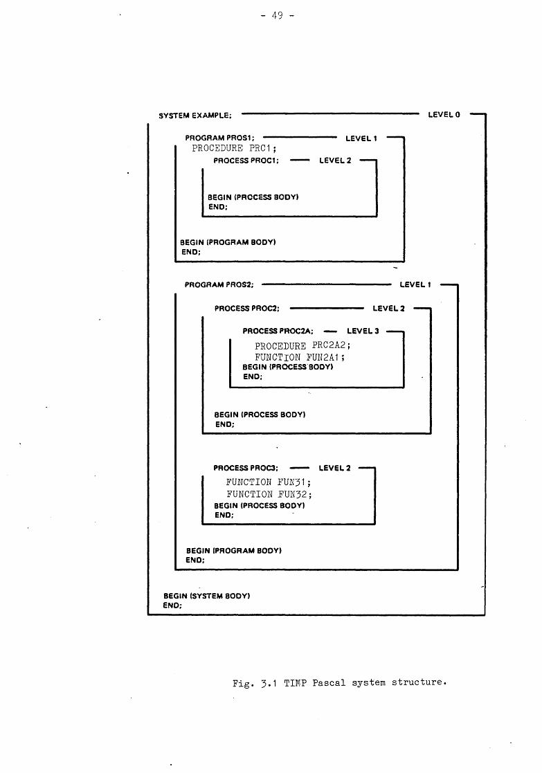
The Pascal language encourages software development by a top-down methodology. The concurrent implementation used in the project is hierarchically structured as shown in Fig. 3-1• The structure is similar to that of Brinch Hansen 18] and is defined in terms of SYSTEM, PROGRAM, PROCESS, PROCEDURE and FUNCTION. This allows the modularity of standard Pascal to be maintained in a concurrent environment.
Partitioning for a multiple processor system is achieved by assigning each concurrent program to a single MPU (Jones and Schwarz [24]). The main disadvantage of this method is that the run-time executive is duplicated in each processor. From the memory map of Fig. 2.1b it can be seen that total memory requirements increase significantly since the run-time executive occupies up to one quarter (16 kbytes) of the memory space of each MPU.
3.2.2 Features of Texas Instruments Microprocessor Pascal (TIMP)
The Pascal software supplied by Texas Instruments [47] is implemented using the UCSD p-System [«] which compiles source programs into a pseudo-code (p-code) for execution by an interpreter. Standard Pascal as defined by Jensen and Wirth [16] has some well known deficiencies and as such most implementations include extra features which serve to increase the utility of the language. In TIMP, the added features which ease program development may be summarised as follows :
1) Concurrency - Concurrency based on the latency of processes is available via semaphores. The semaphores are of the counting type and are manipulated by procedures such as INITSEMAPHORE, WAIT and SIGNAL.
2) Interprocess Communication - In a multiprogramming environment it
49
SYSTEM EXAMPLE; LEVEL 0
PROGRAM PROS1;PROCEDURE PRC1;
PROCESS PROC1;
BEGIN (PROCESS BODY) END;
BEGIN (PROGRAM BODY) END;
LEVEL 1
LEVEL 2
PROGRAM PROS2;
PROCESS PROC2;
LEVEL 1
LEVEL 2
PROCESS PROC2A; LEVEL 3
PROCEDURE PRC2A2;FUNCTION FUN2A1;
BEGIN (PROCESS BODY)END;
BEGIN (PROCESS BODY) END;
PROCESS PROC3; ------- LEVEL 2
FUNCTION FUN31; FUNCTION FUN32;
BEGIN (PROCESS BODY)END;
BEGIN (PROGRAM BODY) END;
BEGIN (SYSTEM BODY) END;
Fig. 3.1 TIMP Pascal system structure.

- 50 -
is necessary to allow communication between processes. In TIMP this is done by communication channels which are either buffers or inter-process files. Communication beween processes can also be achieved by the use of shared variables in which case the user must ensure mutually exclusive access.
3) Modular Programming - Separate compilation is allowed thereby facilitating the creation of libraries and the development of large programs.
4) Memory Management - As well as standard Pascal pointer types and the procedures for their manipulation, facilities are included to specify the heap and stack sizes of programs and processes. These resources can be allocated and reclaimed dynamically during execution.
5) Hardware Dependence - Access is .provided to the hardware features of the CPU in order to allow control of input/output and interrupts. Individual memory locations may be examined and external assembly language routines could be linked to a program.
In common with all other implementations of Pascal under the UCSD p-System, TIMP also differs from standard Pascal in that the passing of procedures and functions as parameters is not allowed.
3*2.3 Other programming languages
The prototyping emulator is provided with a high-level Pascal-based language (AMPL [47]) in which debugging programs may be written. It can be used for debugging both the hardware and software of target systems.
An extended BASIC interpreter is included in the software supplied. Its implementation allows manipulation of the hardware of the host development computer. In the development of the interactive program (this is described in Chapter 4), the string handling and floating point arithmetic (FPA) routines were useful in producing formatted screen displays.

- 51
An assembler is provided for producing machine-code level routines for the TMS 9900 processor. In order to maintain transportability to other systems, the number of assembly language routines has been kept to a minimum. Only in areas such as communication and timing where speed of execution is critical has assembly language been used. It was also found necessary to include a substantial number of machine-code routines in the interactive control program.
3*2.4 Software development process
A wide range of utilities and software tools are available for program development, the most important of which include :-
EDITOR - a screen-based text editor.COMPILER - a Pascal compiler which produces p-code for interpretive
execution.ASSEMBLER - produces relocatable code for the TMS 9900.COLLECTOR - this collects all the run-time support required to
execute Pascal programs on a target MPU.LINKER - links several code segments into an executable module.DEBUGGER - programs can be debugged at the machine-code level or at
the Pascal statement level. Under AMPL programs can be debugged in an emulated target environment.
UTILITIES - a wide variety of utilities to create, read and modify files are available.
The use of these utilities in the development of simulation software is illustrated in Fig. 3*2. For faster execution, a CODEGEN utility is provided for generating the processor native code but this proved to be unreliable. In any case, for power system simulation, most of the time is spent on floating point operations and thus no worthwhile gains are achievable. All the simulation programs therefore execute in the interpretive mode. The efficiency of the implementation is characterised by a set of benchmarks in Appendix A.

52
Fig 3.2 Software development process

53 -
3-3 COMMUNICATION BETWEEN COOPERATING PROCESSES
Synchronisation and communication functions are usually implemented at a low level and are thus 'invisible' to the user. The intention here is to develop a 'visible' multiple processor system whose architecture can be exploited by the user. This means that the user should be able to explicitly specify communication between processors. Such a system was developed by Halsall and others [25] who used a set of communication primitives based on the rendezvous concept. In a distributed system for mining applications (CONIC [5l])> use was made of message passing protocols to control equipment distributed over a coal mine.
3-3-1 Structuring Concepts in Parallel Processing
The earliest concurrent processes were implemented with hardware interrupts to achieve switching between a main computational task and its I/O related processes. Further development has resulted in the present-day time-sharing operating systems which manage the allocation of computer resources (mainly CPU time) between several users, seemingly simultaneously. The task of writing such operating systems is much simplified by using Dijkstra's bottom-up approach [48].
Synchronisation is required when different processes are required to perform certain tasks in some sequence. If a section of code may not be executed until some condition becomes true then conditional synchronisation is required. If a section of code must be executed without interruption then mutual exclusion is required. While the concept of synchronisation may be used to resolve all the possible problems of interference, sequencing or deadlock that may occur, certain operations are most efficiently effected by passing messages between processes (Hoare [22]). This is especially true in a multiple processor system where explicit communication is required anyhow.

- 54 -
3-3-2 Synchronisation and communication mechanisms
In choosing an appropriate set of mechanisms for synchronisation and communication between several processors, proper consideration must be given to the hardware architecture. Some mechanisms may be wholly inappropriate in certain systems. For example, in systems without common memory, the widely used tool of inspecting and updating a memory location is expensive to simulate. In an attempt to circumvent the problem of choosing between the various available methods of achieving synchronisation, Hoare [22] proposed input and output commands for communication between sequential processes.
In Hoare's implementation, synchronisation is implicit in that an input or output command is delayed until the corresponding remote output or input command is executed. In a general purpose distributed operating system, this method of synchronisation works well since any processor that is blocked on an I/O command can switch to some other ready process. However, synchronous message passing can result in idle processors if there are no waiting processes or, excessive overhead if context switching is expensive.
In Table 3.1, some synchronisation mechanisms are listed according to their implementation levels. The mechanisms at the low, medium and high levels are usually defined as operating system primitives. At the very high level, the operations of the mechanisms are user-defined to suit specific applications (see [18—253)-
3.4 DISTRIBUTED MONITORS FOR INTERPROCESSOR COMMUNICATION
3-4*1 Structure
Interprocessor communication is based on the monitor construct [l8,2l]. Due to the need for explicit cooperation between communicating MPUs, the implementation may ’ be best described as a distributed monitor. The

Table 3-1 Communication and synchronisation primitives
IMPLEMENTATIONLEVEL
ELEMENT OPERATIONS COMMENTS
Hardware Interrupt H/W flag
enable/disable test and set,
reset
priority queuing mutual exclusion
Low Lock variable lock/unlock busy waiting
Medium Semaphore Critical region
signal/waitenter/exit
implicit queuing mutual exclusion
High Monitor procedure call implicit queuing, mutual exclusion, signalling
Conditional critical region user defined as for monitor
Very high Path expression user defined as for monitor
Rendezvous or Remote
procedure call
Input/output client/servertransactions

- 56 -
various primitives are implemented using the concept of the virtual machine ([48]) and the hierarchical structure is illustrated in Fig. 3.3
within the context of a user application program.
Level 1 of the hierarchy is the electrical interconnection as described in Chapter 2. At level 2 the hardware mechanisms available such as interrupts and hardware flags are manipulated to achieve synchronous word-parallel transfers. Buffer management and synchronisation are at level 3* The user-accessible communication primitives are implemented at level 4 and the application program is at level 5«
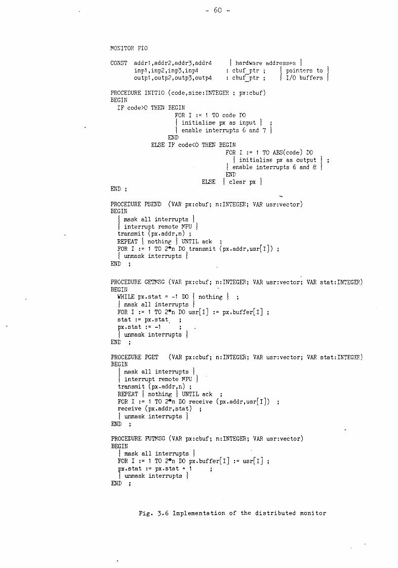
3«4«2 Implementation
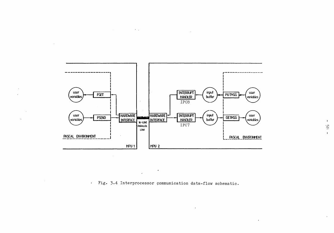
The distributed monitor is written in assembly language for maximum speed and flexibility in handling the hardware and occupies a total of 500 bytes. The actual message transfer mechanism, as explained in Chapter 2, is synchronous and the software routines on either side of the communication channel are accurately timed such that synchronism is maintained for the longest messages that could be sent. Fig. 3.4 shows a schematic of the data-flow between two MPUs. Communication is initiated by the procedures PSEND and PGET with IPC7 and IPC8 respectively being the interrupt service routines. Exclusive access to the local buffers is provided by the procedures GETMSG and PUTMSG. Typical declarations of data structures for the message buffers are shown in Fig. 3*5*
Transmit and Receive Buffers
User Buffer
port address status count message buffer
array of reals typical only
TYPE vector = ARRAY [l..nmax] OF REAL ; cbuf = RECORD
addr,status,count : INTEGER ;buffer : VECTOR
END ;
Fig. 3*5 Port and message buffer data structures

57 -
Fig. 3*3 Hierachical structure of the distributed monitor.
Ivni
Fig. 3.4 Interprocessor communication data-flow schematic

- 59 -
From the user's viewpoint, interprocessor communication is achieved through local monitors which handle the communication channels and the associated buffers as system resources. The implementation logic of the monitor as seen by the user is given in Fig. 3*6.
For flexibility, the data structures for the buffers are defined within the Pascal environment. Although unrestricted access to the buffer is therefore possible, mutual exclusion is not guaranteed. However, the buffer status may be safely read (e.g. to check if the execution of a GETMSG statement will result in blocking).
3-4.3 Message-passing primitives
The various procedures of the monitor are now described and their interface with the Pascal language application programs outlined. The communication between two MPUs representing a network and a generator is used as an example.
1. Initialisation - Before the monitor procedures could be used, the embedded data structures' (port addresses and message buffers) must be initialised. This is achieved by the procedure INITIO which enables interrupts and configures the ports to the user's requirements. A typical initialisation call is
INITIO (Nport,length,msgbuffs)which specifies the number of ports to be initialised, their length and the address of area of memory reserved for the buffers. Buffers that have already been initialised may be cleared by setting the value of Nport to zero.
2. Message sending - Messages within buffers in the Pascal environment may be sent to a remote MPU by invoking the monitor procedure PSEND* As shown in Fig. 3*6, an interrupt is generated in the remote MPU and after initial handshaking, the contents of the message buffer are transferred to the receive buffer of the addressed MPU. A typical call to the
60
MONITOR PIO
CONST a d d r l ,a d d r 2 ,a d d r 3 ,a d d r 4 i n p 1 , in p 2 , in p 3 , in p 4 o u t p ! ,o u t p 2 ,o u t p 3 ,o u t p 4
c b u f_ p tr c b u f p t r
p o i n t e r s to I/O b u f f e r s
PROCEDURE INITIO (code,size:IN TEG E R ; p x rcb u f)BEGIN
IF code>0 THEN BEGINFOR I := 1 TO code DO { i n i t i a l i s e px as in p u t j ;| e n a b le i n t e r r u p t s 6 and 7 }
ENDELSE IF code<0 THEN BEGIN
FOR I := 1 TO ABS(code) DO j i n i t i a l i s e px as output
{ en a b le i n t e r r u p t s 6 and 8 END
END ;ELSE | c l e a r px
PROCEDURE PSEND (VAR p x r c b u f ; n:INTEGER; VAR u s r : v e c t o r ) BEGIN
| mask a l l i n t e r r u p t s ]{ i n t e r r u p t remote MPU } t r a n s m it ( p x .a d d r ,n ) ;REPEAT | n o th in g ] UNTIL ack ;FOR I := 1 TO 2*n DO tr a n s m it ( p x . a d d r , u s r [ l ] ) ;{ unmask i n t e r r u p t s }
END ;
PROCEDURE GETMSG (VAR p x r c b u f ; n:INTEGER; VAR u s r r v e c t o r ; VAR statrINTEGER) BEGIN
WHILE p x . s t a t = -1 DO | n o th in g j ;{ mask a l l i n t e r r u p t s jFOR I := 1 TO 2*n DO u s r [ l ] := p x . b u f f e r [ l ] ; s t a t := p x . s t a t ;p x . s t a t := -1 ;{ unmask i n t e r r u p t s j
END ;
PROCEDURE PGET (VAR p x r c b u f ; n:INTEGER; VAR u s r r v e c t o r ; VAR stat:INTEGER) BEGIN
j mask a l l i n t e r r u p t s ] j i n t e r r u p t remote MPU } t r a n s m it ( p x .a d d r ,n ) ;REPEAT { n o th in g } UNTIL ack ;FOR I := 1 TO 2*n DO r e c e i v e ( p x . a d d r , u s r [ l ] ) ; r e c e i v e ( p x . a d d r , s t a t ) ;{ unmask i n t e r r u p t s }
END ;
PROCEDURE FUTMSG (VAR p x r c b u f ; n:INTEGER; VAR u s r r v e c t o r )BEGIN
{ mask a l l i n t e r r u p t s }FOR I := 1 TO 2*n DO p x . b u f f e r [ l ] := u s r [ l ] ; p x . s t a t := p x . s t a t + 1 ;j unmask i n t e r r u p t s }
END ;
F i g . 3»6 I m p l e m e n t a t i o n o f t h e d i s t r i b u t e d m o n i t o r

- 61
monitor from the program in a generator MPU isPSEND (Network, number, currents)
where the port name of the remote MPU has been designated Network. In addition to the message transfer rate of 30 microseconds per 16-bit word quoted in Chapter 2, an overhead of 720 microseconds is incurred whenever this procedure is called. The remote interrupt service routine executes with an overhead of 100 microseconds plus 30 microseconds per word.
Secure access to the communication buffer in the receiving MPU is achieved by the use of GETMSG. This procedure allows exclusive access to the buffer by the use of a conditional wait. Thus if there is no new message present in the buffer the calling process is blocked. Non-blocking access may be achieved by checking the buffer status before entering the monitor (similar to the input guard concept of Dijkstra [48]). In the above example of a generator MPU sending currents to a network MPU the corresponding receipt by the network MPU would be
GETMSG (generatorl, number, currents, status) where the status variable may be checked to determine if any messages have been lost. If this procedure is not blocked, a memory-to-memory transfer takes place at a rate of 17 microseconds per 16-bit word plus an overhead of 600 microseconds.
3. Message retrieval - Messages within the transmit buffers in a remote MPU may be retrieved by invoking the monitor procedure PGET. An interrupt is generated in the remote MPU and, after handshaking, the contents of the transmit buffer are transferred to the Pascal buffer of the calling MPU. A typical call to the monitor is
PGET (generatorl, number, currents, status)The status parameter may be checked to determine whether the message received is old or new, or whether any messages have been lost.
The transmitting buffers of the remote MPU may be securely updated by the procedure PUTMSG. This procedure is non-blocking and it may be necessary to check the status of the buffer before putting in a new message in order to avoid overwriting a previous message that has not yet been retrieved. An example of updating the buffer within a generator

- 62
MPU may be expressed asPUTMSG (network, number, currents)
The execution rates of PGET and PUTMSG are similar to those of PSEND and GETMSG respectively.
The distributed monitor may be linked to the concurrent environment of TIMP by associating incoming interrupts with semaphores. Idle time is then reduced since lower priority processes will be executed wlen blocking occurs. Mutual exclusion is maintained by virtue of the fact that the monitor resides outside the Pascal environment. Thus the monitor primitives appear as indivisible operations to the run-time executive. This feature was used by Lopez [42] in implementing concurrent multi-rate integration methods.
3-4»4 Higher level communication protocols
For the purpose of applications programming the procedures of the distributed monitor described above may be regarded as primitive operations. In order to facilitate programming, these procedures can be used to construct higher level protocols which are useful for specific applications. Examples of such protocols are given below.
1 ) Broadcast - In cases where the central MPU of a star configuration needs to transmit the same message to all peripheral MPUs, a suitable protocol is the Broadcast. Typically, this may be implemented as
PROCEDURE Broadcast (message,length) ;VAR port : ARRAY [l..n] OF cbuf ;BEGIN
FOR I := 1 TO n DO PSEND(port[l],length ,message) END ;
2) Receive-All - This procedure may be required if the central MPU is to receive updated values from all the peripheral MPUs. The problem is slightly more complex since the GETMSG procedure is blocking. Thus if

- 63 -
the first GETMSG executed happens to require data from the slowest MPU then all the others would be kept waiting. It is then necessary to U3C an input guard (Dijkstra [48], Hoare [21]) before each GETMSG to find out whether the procedure would block. This is implemented as follows:
PROCEDURE Receive-All (portl,port2,port3) ;VAR got1,got2,got3 : BOOLEAN ;BEGIN
got1 := FALSE ; got2 := FALSE ; got3 := FALSE ;REPEAT
IF (NOT gotl) AND (portl . statOO) THEN BEGIN
( get message from portl j got1 := TRUE
ENDELSE IF (NOT got2) AND (port2.statOO) THEN
BEGIN{ get message from port2 ] got2 := TRUE
ENDELSE IF (NOT got?) AND (port3.statOO) THEN
BEGIN{ get message from port3 } got3 := TRUE
ENDUNTIL gotl AND got2 AND got3
END ;
This is equivalent to the SELECT statement of ADA (USDOD [19]). In particular situations, such as when the central MPU solves a network and the peripheral MPUs solve generators, it may be advantageous to do some processing as soon as a message is received. This minimises the network idle time since some processing is done in parallel with the slowest MPU after the receipt of the first message.
3) Send-wait-reply - In transaction processing a client requests a service and then awaits a reply. This is the mechanism suggested by Hoare for communicating sequential processes [22] and implemented in ADA as the rendezvous [l9,23]• This is quite simply implemented as:

CLIENT
PROCEDURE Send-wait-reply ;BEGIN
PSEND(server,length,request);[ busy-waiting j ;
GETMSG(server,length,reply,st) END ;
SERVER
PROCEDURE Respond ;BEGIN
GETMSG(cl ient,length,request,st);{ process request } ;
PSEND(client,length,reply)END ;
4) PSIGNAL/PWAIT - The monitor procedures have been designed such that synchronisation is implicit. For program clarity, notation has been included for pure signalling operations. Adopting Hoare's definition of a data structure without values as a signal [22], a PSIGNAL may "be defined as sending a message of zero length. The corresponding PWA1T operation is achieved by the procedure GETMSG extracting a message of zero length from the local buffer.
PROCEDURE PSIGNAL (portx : port_name) ;VAR aux_buff :cbuf ;BEGIN
PSEND(portx,0,aux_buff)END ;
PROCEDURE PWAIT (portx : port_name) ;VAR aux_buff :vector ;
stat :INTEGER ;BEGIN
GETMSG(portx,0,aux_buff,stat)END ;
Since no message is transmitted only the buffer status flag changes. Consequently, the procedures are very fast; a PSIGNAL is executed in 200 microseconds and a non-blocking PWAIT in 160 microseconds. These compare with an execution time of 830 microseconds for each call to the standard SIGNAL and WAIT procedures (see Appendix A).

- 65 -
3-5 PROGRAMMING FOR PARALLEL EXECUTION
3-5-1 Factors causing loss in performance.
The cost of parallel solutions may be measured in terms of time and space. The cost in space is determined by the method of partitioning used and the type of hardware architecture. In our case a substantial amount of memory is required due to the duplication of the run time executive. In some true multiprocessors (ETH [7]), many processors may use the same copy of a section of code but this results in a significant penalty due to contention [23-25]-
The analysis of cost in terms of time requires identification of the different factors which result in slower solutions. The most important of these are shown in Fig. 3-7* The loss in performance is due to both the penalty of decomposing a problem for solution in two or more MPUs, and the cost of implementation on a particular multiple processor system. These two penalties may be further divided into two parts whose effects are first and second order.
Implementation penalty - this can be directly related to specific characteristics of the hardware architecture and system software of the multiple processor system. The time each MPU spends waiting to synchronise with other MPUs is responsible for the greater part of the implementation penalty and is a first order effect. Depending on the type of communication mechanism used, two equal processes may slow each other down due to the need to synchronise.
The time required for communication results in each MPU doing an extra amount of work but this is typically very small. However, if a large number of messages have to be sent, the total time spent on communication may become appreciable. In addition, contention may occur and cause some MPUs to wait. In general, loss in performance due to communication can only be regained by the use of faster hardware.

TIME
- 66
loss in performanceiijiii
implementationpenaltyii
iidecomposition
penaltyiii ii i
synchronisation jtime jiiii
communicationtime
i it iunequal jpartitions |iiii
partitioningoverhead
a) Factors causing loss in performance.
NETWORK MPUDAT̂ A
TRANSFER
DATA^TRANSFER
GEN. MPU
Idle time OverheadSynchronisation time Communication time
Unequal partitioning Partitioning overhead
Useful computation
b) Idle time and overhead in one computation step
Fig. 3*7 Implementation and decomposition penalties

- 67 -
Decomposition penalty - the larger part of this penalty is due to problem decomposition that results in unequally loaded MPUs. This may limit the overall execution time to that of the slowest MPU.
Partitioning overhead is a second order factor due to decomposition. There are several sources including, duplication of overheads found in serial programs such as accessing arrays, calling procedures etc., any data collection required and extra calculations due to partitioning. Very little can be done about such overheads since they are either inherent in the sequential process or are necessary to realise a parallel solution.
Note that the second order effects result in a computational overhead whereas the first order effects cause idle time. Also in more complex systems, it may be possible to identify some third order effects such as partial lockout and overhead due to detection and recovery from deadlock.
3-5-2 Time-dependent errors
A consequence of implementing flexible communication primitives is the possible occurrence of undesirable time-dependent phenomena which are difficult to detect. Some common errors of this type are identified below and an indication is given of how they may be avoided.
Deadlock - It is useful to distinguish between the two types of deadlock that may occur in parallel or concurrent systems as shown in Fig. 3-8. We refer to deadlock involving two MPUs as the 'deadly embrace' (Dijkstra [48]) and that involving three or more MPUs as the 'circular wait’. The deadly embrace is easier to detect and may be avoided between any two MPUs by following the simple rule that neither MPU may execute two consecutive GETMSG statements. In the case of the circular wait, deadlock can only be avoided by careful programming.

68 -
Waitingfor A
for B
a) Deadly embracefor C
b) Circular wait
Fig. 3*£ Types of deadlock
Message overrun - A second type of error occurs when an MPU sends messages fast enough to overwrite unconsumed messages. The solution to this problem is similar to the deadlock avoidance scheme above in that an MPU may not execute two consecutive PSEND statements.
Lockout - This third form of time-dependent error occurs when an MPU receives high priority interrupts at a fast enough rate to prevent it acknowledging an MPU that is interrupting at a lower priority. In the power system application programs total lockout cannot occur since all the MPUs must synchronise at the end of each simulation step. However, partial lockout is possible when large numbers of processors are used.
Crawling - Logically correct.programs may perform badly due to the misuse of some primitives. The phenomenom of crawling occurs when an MPU generates several inter-processor interrupts while waiting for some condition to become true. For example, execution of a statement such as
REPEAT PGET(portx,...,stat) UNTIL stat=0 will result in 1 0 % drop in execution speed of the remote MPU until it updates its buffer.
3-6 ANALYSIS OF A PARALLEL ALGORITHM
Several analytical techniques exist which may be used to predict the performance of parallel algorithms on multiple processor systems. In the absence of a specific hardware system Brasch and others [37], and Fong and Pottle [ll] simulated the performance of proposed algorithms on various architectures. The purpose of this analysis is to identify possible problem areas and their solutions.

- 69 -
3-6.1 Problem description
The problem under consideration is the transient stability analysis of a power system. A simple physically-based task decomposition is assumed whereby the algebraic equations representing the network are solved on one MPU and each generator has its differential equations being solved on a single MPU. The mathematical models and solution methods will be treated in later chapters. For the present, we assume a step-by-step algorithm where the network MPU calculates the voltages at the generator busbars and the generator MPUs calculate current injections into the network. Thus during each time-step the network MPU sends voltages to the generator MPUs and receives their currents injections.
An appropriate configuration of MPUs for the algorithm is a 'star' with the network in the central MPU as shown in Fig. 2.3c. Timing diagrams of one step of the algorithm are given in Fig. 3-9& and b. These illustrate the two possible computation patterns depending on the relative computation times the MPUs require between receiving data and being ready to send data. In the subsequent analysis, it is assumed that the generator programs are identical and execute in the same time.
3-6.2 Some performance measures
A common measure used in evaluating the performance of multiple processor systems is the speed-up factor which is defined as:
speed-up - TserjLa-̂ /Ta c .̂ua2 (5*1)
where T is the computation time on one MPU and Tac^ua-̂ the time onN MPUs. For analytical purposes insight may also be gained by considering the overall efficiency of the computation which is defined as
efficiency = speed-up/N (3-2)
With reference to Fig. 3-7, the speed-up factor may be calculated from the following equation

NETWORK GEN. 1 GEN. N NETWORK GEN. 1 GEN. II
P S END GETMSG ///// i d l e //■/,/ - / / / T I M E ////// M
••11l111
PS END GETMSG
■ M------
DATATRA N SFER
IN T E R R U P T111111l
PS EN D
. - . I N T E R R U P T - -P S EN D
P I 1/'// I D L E ////W "/vM'//M /m W M W /,
W ////////M
•
G E T : D A T A ■
a ) S i n g l e - s t a g e c o m p u t a t i o n p a t t e r n b) D o u b l e - s t a g e c o m p u t a t i o n p a t t e r n
Fig. 5*9 Typical computation patterns.

71
Tn + (N -1)*Tg
speed-up = --------------- (>3)
max ^net’̂ gerJT , = T + T + T + T + 2*T *(N-1)net nsr nrs nov nid c v '
T = T + T + T + T . , + P*Tgen gsr grs gov gid c
The various times for the generator and network MPUs are
T ,T - total computation time in serial algorithmO 11
TgSr>Tnsr " computation time between sending and receiving data
Tgrs,Tnrs " computation time between receiving and sending data
TgOV,Tnoy - partitioning overhead
Tgid>Tnid ~ idle time due to synchronisation
Tq - time required to send or receive data
Analysis of computation patterns
An analytical study was carried out in order to gain insight into the effect of various factors on the efficiency of the model multiple processor system. Curves of efficiency and speed-up are plotted to demonstrate the effect of various parameters.
A synchronous communication scheme is unacceptable since idle time is almost always incurred. Its effect can be seen in Fig. 3»10 where two equal processes slow each other down due to the need to synchronise. As shown if asynchronous communication routines are used then it is possible to eliminate this idle time.
In the case of a transient stability study using as many MPUs as there are generators and one MPU for the network, the loading of the network MPU is critical. If it is slower than a generator MPU the system suffers a sharp drop in performance as shown in Fig. 3»11a«
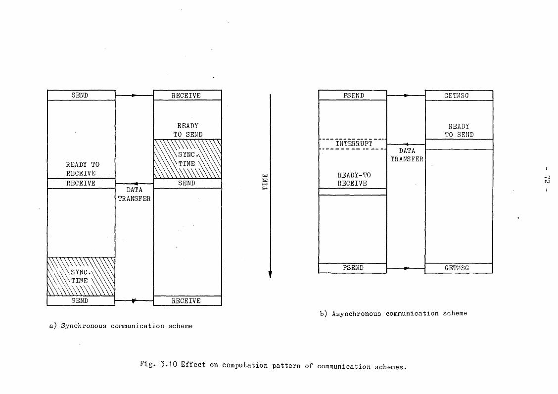
a) Synchronous communication scheme
PS END GETMSG
READY TO SEND
INTERRUPTDATA
TRANSFER
READY-TORECEIVE
PSEND GETMSG
b) Asynchronous communication scheme
Fi-S* 3• 10 Effect on computation pattern of communication schemes.

SPEE
D-UP
----->
73
Fig. 3.11 Performance curves for single-stage computation

74
As the number of processors grows, increased overhead may affect the partitioning and cause idle time; this is the phenomenon! responsible for saturation when extra processors are added as shown in Fig. 3*11b. In actual systems, the overhead tends to grow faster than proportionally; this eventually leads to an absolute reduction in performance.
In the preceding example, it was assumed that Tnsr > ^grs* The opposite is more likely to be the case and the distribution of idle time is as shown in Fig. 3* 9b. For a large number of MPUs, the phenomenom of partial lockout may occur if some generator MPUs are allowed to send results before the network MPU has finished updating them all. This may be cured by masking all interrupts in the network MPU while it sends. The effect of partial lockout on computation efficiency and speed-up is illustrated in Fig. 3*12.
3*6.4 Implications for large systems
The simple model considered here requires the network equations to be solved in a single MPU. In large systems between a third and half of the total computation time is required to solve the network [36,37]* It is therefore necessary to reduce the network solution time to the same order as that of a generator or group of generators. This can be done by the use of parallel solution techniques [9-11,41] on an architecture such as that proposed in Section 2.5.
The behaviour of such a system would be similar to the model analysed here. The effect of communications overhead would be reduced due to the presence of multiple communication paths but partitioning overhead would increase, especially in the network solution.
3-7 CONCLUSIONS
The software resources available for application programs have "been described. The modularity of Pascal, its data structuring facilities and

SPEE
D-UP
----->
EF
FICI
ENCY
- 75 -
Fig. 3*12 Performance curves for double-stage computation

- 76 -
the extensions included in TIMP have been found to be well suited to the development of an environment in which parallel processing algorithms may be implemented.
Synchronisation and communication primitives in concurrent programs and distributed systems is still an active area of research. As there are no universal criteria for choosing the most suitable constructs for a given application, the approach adopted in this work is that of selecting those which best suit the existing hardware. This concurs with Hoare's conclusion that no set of primitives can be excluded from consideration if they can be implemented efficiently and shown to be appropriate to the task in hand [22]. The generality of the distributed monitor has been demonstrated in that other constructs may be realised using its primitive operations.
A computation model has been proposed for analysing the behaviour of the parallel processing scheme and shown to be useful in predicting the effect of changes in the partitioning of the computational task. From the analysis we may conclude that :
a) asynchronous communication primitives are to be preferred to synchronous schemes.
b) efforts should be made to confine any idle time incurred to the central MPU.
c) when interprocessor interrupts from several MPUs are resolved by a priority scheme, it is possible for partial lockout to occur. Changes in the communication scheme may be required to avoid this.
The implementation of a monitor for interaction is described in Ch. 4
and the application of the communication procedures described here to power systems simulation will be given in Chapter 7.

77
CHAPTER 4
INTERACTIVE COMPUTATION
4.1 INTRODUCTION
Research so far into multiple microprocessor arrays for power systems has not addressed the problems of input/output or user interaction. Brasch et al. [37] envisaged their parallel system being attached to a host mainframe computer as a special-purpose processor. In such a configuration using array . processors, Orem and Tinney [34] found that the cost effectiveness of the combination was much reduced due to the relatively slow data transfer rates between the host computer and an array processor. Similar considerations led Detig [36] to conclude that attached scientific processors are unsuitable for power system applications.
In the system developed here, a host minicomputer based on the same processor used in the multiple processor system is used for I/O and user interaction. This is efficient for dedicated systems, since the problems of providing high speed interfaces to a general purpose host computer are avoided.
This Chapter outlines the design and implementation of an interactive program which was written to enable a user to control the simulator from the host minicomputer. A description of the interactive program and its features is given. Finally, the steps required to set up, execute and control applications programs in the interactive environment are explained.
4.2 MAN/MACHINE AND MACHINE/MACHINE INTERFACES
4*2.1 Models of human behaviour
In the design of man/machine interfaces (MMI), it is useful to define conceptual models of the various roles man may play in an interactive system (Rouse [51,52],Carey [53]). In power system computation two suitable models are :
(i) operator - for on-line control systems or real-time simulators, (ii) analyst - appropriate in the context of research or design.
This dichotomy is exemplified by comparing the interactive package described by Undrill et al. [39] which is based on the requirements of an analyst, . with the advanced dispatcher training simulator by Podmore and others [54] where the needs of the operator dominate. However, the interactive systems described by Stagg [38] indicate that a comprehensive system should cater for both roles.
A third model that warrants consideration is that of the 'student'. The training simulator designed by Podmore et al. [54] incorporates an instructor's console, but experience with a similar training simulator in Japan [56] has highlighted the need to reduce the workload of instructors. A recent survey by a CIGRE working group [55] identified a growing need for educational tools in training operators. It is proposed here that this need should be satisfied, not only implicitly by training on a real-time simulator, but also by explicit computer-aided instruction.
4.2.2 Interaction patterns
In designing general-purpose interactive simulators, it is necessary to consider the three models of student, operator and analyst. This results in a multi-mode system although more emphasis may be placed on one aspect. Irrespective of the role models on which a system is based, interactive computation comprises the four basic steps listed in

- 79 -
sequence in Table 4*1 with some typical activities. Operator-modelled systems primarily require on-line interaction whereas the activities of program preparation, program control and post-processing are usually to be found in analyst-modelled systems. A student-modelled system would require a substantial amount of post-processing.
Table 4.1 : Sequence of interactive computation
STEP TYPICAL ACTIVITIES
1. Program preparation- data preparation- choice of models- choice of solution methods
2. Program control- run, pause, stop- command files- on-line interaction
3. On-line interaction- parameter modifications- schedule events- program control
4. Post-processing- report preparation- curve plotting- statistical analysis
In actual systems, this sequential view of computation is complicated by the addition of concurrency. Thus in real-time systems where several tasks must be executed simultaneously, it is necessary to take into account the response time required for each task. In a study of appropriate task allocation in flight control systems, Rouse [52] considered in detail the modes of interaction that occur, in an operational environment (see Fig. 4.1a). He defined a covert mode of interaction as that in which the intervention of the control computer is not obvious.
Fig. 4»1b is an equivalent representation of the power system simulator. The system comprises the dynamic simulator, the host minicomputer and a human user. The data flow diagram of a single transaction is given in Fig. 4.1c. Data input by the user is followed by program execution and

80
a) Nodes of man/machine interaction (Rouse [52J)
’b) Interactive control of simulator
C) Single transaction data flow
Fig. 4.1 Data flows in man/machine interaction

81
results output by the computer. The loop is closed when the userevaluates the results and inputs more data.
4-2.3 Dialogue types
The six basic man/machine dialogue types with which more complex dialogues may be defined are identified in Table 4-2. A typical session starts with data being input and ends with results being output. During the program execution, the user may enter commands which the machine executes; similarly the machine may print out messages to which the user reacts. Such transactions are basically monologues since either party may choose not to reply. True dialogue takes place when’queries must be answered before execution can continue.
Table 4-2 : Man/machine dialogue types
MAN MACHINE EXAMPLE
input data --- > computecommand --- > executequery <-- > replyreply <-- > queryrespond <--- reportevaluate <--- output data
send data, modify parameters halt, event scheduling display request program prompterror message, status report plot, monitor
4-2-4 A model of interactive computation
The above concepts can be combined into the hierarchical model of interactive computation given in Fig. 4-2. All interactive programs include some or all aspects of the model. The innermost level labelled INFORMATION requires the fastest response whereas COMPUTATION can proceed at a slower rate. COMMAND-AND-CONTROL is intermediate between these with response times being determined by the operator or the controlled system. Table 4-3 lists some correlations between various system design parameters. As an indication of how these ideas are utilised, consider the implementation of the dynamic simulator.
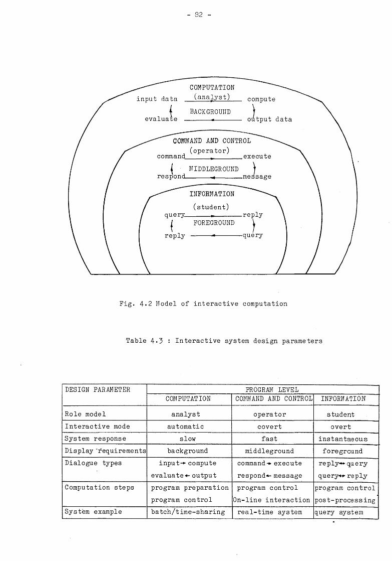
82
Fig. 4*2 Model of interactive computation
Table 4*3 : Interactive system design parameters
DESIGN PARAMETER PROGRAM LEVELCOMPUTATION COMMAND AND CONTROL INFORMATION
Role model analyst operator studentInteractive mode automatic covert overtSystem response slow fast instantaeousDisplay 'requirements background middleground foregroundDialogue types input-* compute
evaluate«- outputcommand-* execute respond*- message
reply** query query** reply
Computation steps program preparation program control
program control On-line interaction
program control post-processing
System example batch/time-sharing real-time system query system

- 85 -
The basic computation loop is analyst-modelled. Once the parameters of a study have been specified, interaction between the host and simulator is automatic. The study completion time is slow and if the user initiates other tasks, the display of results may be relegated to the background.
On-line interaction with the simulation is operator-modelled. The mode of interaction is covert in that commands refer to the power system under study without obvious intervention by the host. The specification of display requirements as "middleground" means that the effect of a command may not elicit an explicit response but may be inferred from subsequent behaviour (e.g. power changes after application of a fault).
The facilities based on a student model are limited but include the capability to inspect data files during the simulation. It should also be possible to program command files without any parameters; the user may then be prompted during execution for the appropriate values.
4*2.5 Input/output devices and communication
The man/machine interface is via the keyboard and screen of the host minicomputer. Menu-driven single-key commands are used for input and a non-scrolling formatted screen is used for output. Input data may be read from disk files and output data may be sent to a printer or graphics terminal. Alternative I/O devices which may be used to good effect include light pens, joysticks, analogue displays and graphics terminals [51-55>57]. Integrating such devices into an interactive environment is merely a data processing task which should be much simplified by software standards such as the ISO draft graphical kernel system (GKS [57])-
The machine/machine interface between the parallel MPUs and the host minicomputer is implemented by interrupt-driven communication over serial lines. The minicomputer may be linked to any or all of the MPUs through the software controlled switch. Dialogue between the machines is by messages with identifying headers.

- 84
4-5 DESCRIPTION OF THE INTERACTIVE PROGRAM
The interactive program has been developed as a set of concurrent modules which are activated either by keyboard input or interrupts from the input/output ports. Most of the routines have been written in assembly language in order to achieve a fast response to inputs. However, a set of driver routines was written in BASIC in order to make use of various high level procedures. The program comprises the following modules:
1) DRIVER ROUTINESThe driver routines carry out all the system initialisation when the system is first loaded. It contains routines to load the object file of the assembly language modules. All data input and the conversion of real numbers to their internal representation is handled by this module.
2) COMMAND PROCESSORThis module polls the keyboard for command inputs or reads commands from a disk file. The commands are then interpreted and the relevant routine is activated. Software control of the programmable switch is implemented in this module.
3) VDT UTILITIESThis module comprises a collection of routines to control the display terminal. Functions such as highlighting, clearing the screen, cursor control and the display of graphics characters are included.
4) FILE HANDLERAll file access is achieved through the routines in this module. Use is made of the operating system for reading from and writing to disk files and error detection.

- 85 -
5) DISPLAY PROCESSORThe initialisation, updating and printing of user status displays are done in this module.
6) COMMUNICATION PACKAGEThe interrupt routines and data structures required for communication via the input/output ports are to be found in this module.
The main function of the control program may be regarded as that of directing a set of input data streams to a set of output devices as specified by the user. This is depicted in Fig. 4*3 where the effect of various commands on input data may be observed. Foreground tasks have exclusive access to the screen while other tasks so indicated may execute concurrently in the background.
4-4 DESCRIPTION OF COMMANDS
4-4.1 Command structure
The interactive control program is menu-driven. Commands are arranged in a tree structure (see Fig. 4*4) and may be selected by a single key stroke from a set of special function keys. At. all times the last line of the screen displays the current commands corresponding to the function keys. When a command is selected, confirmation is provided by highlighting its label. The appropriate action is then performed, or more information is requested either by a prompt or the display of a new set of commands lower in the hierarchy.
4-4.2 Control and initialisation commands
These commands allow the user to set up and control the operation of the simulator. Commands are included to reset, halt and select the mode of
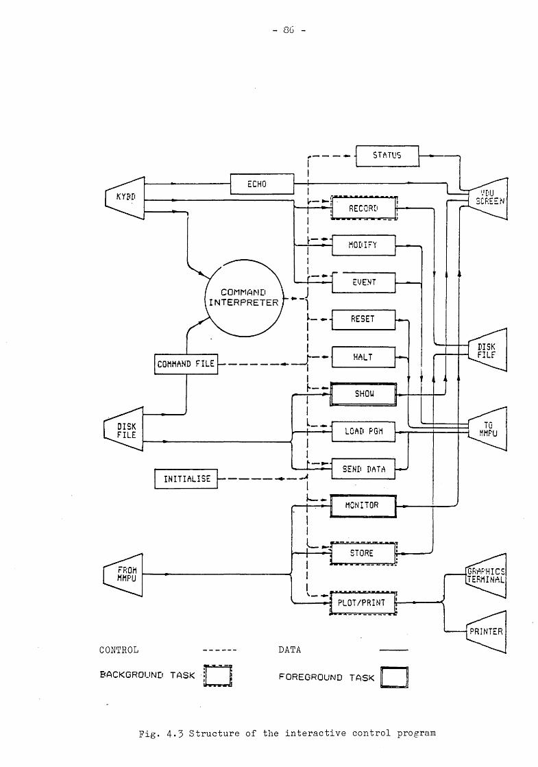
- 86
STATUS
CONTROL DATA
BACKGROUND TASK FOREGROUND TASK
Fig. 4.3 Structure of the interactive control program

SETUP MODEF1 F2 F3 F4 F
SETUP INIT RECX)RD PLOT STORE J STATUS CMDETL SHOW 1
I 1MPU1*
MPU2*
MPU3*
MPU4*X’
MPU5 STATUS EXIT E>IT
1 NEXTP PREVP MARK RETURN TOP MIDDLE BOTTOM EX3
*USER-DEFINED NAMES
SIMULATION MODE 4 F5 F6 F7 F8
] SMJL LOAD SENDAT RESET HALT MONIT MODIFY eve:d
*MPU1
*MPU2 MPU3
*MPU4
*MPU5 MONIT m i HR § _
_
>BL
f *' VAR1 VAR 2* *VAR3
•*VAR 4
*VAR 5 VAR 6 MODIFY EX►IT
*EVT1 EVT2* EVT3* EVT4*
*EVT5 EVT6* EXIT EVENT
co
F i g . 4 . 4 Command t r e e .
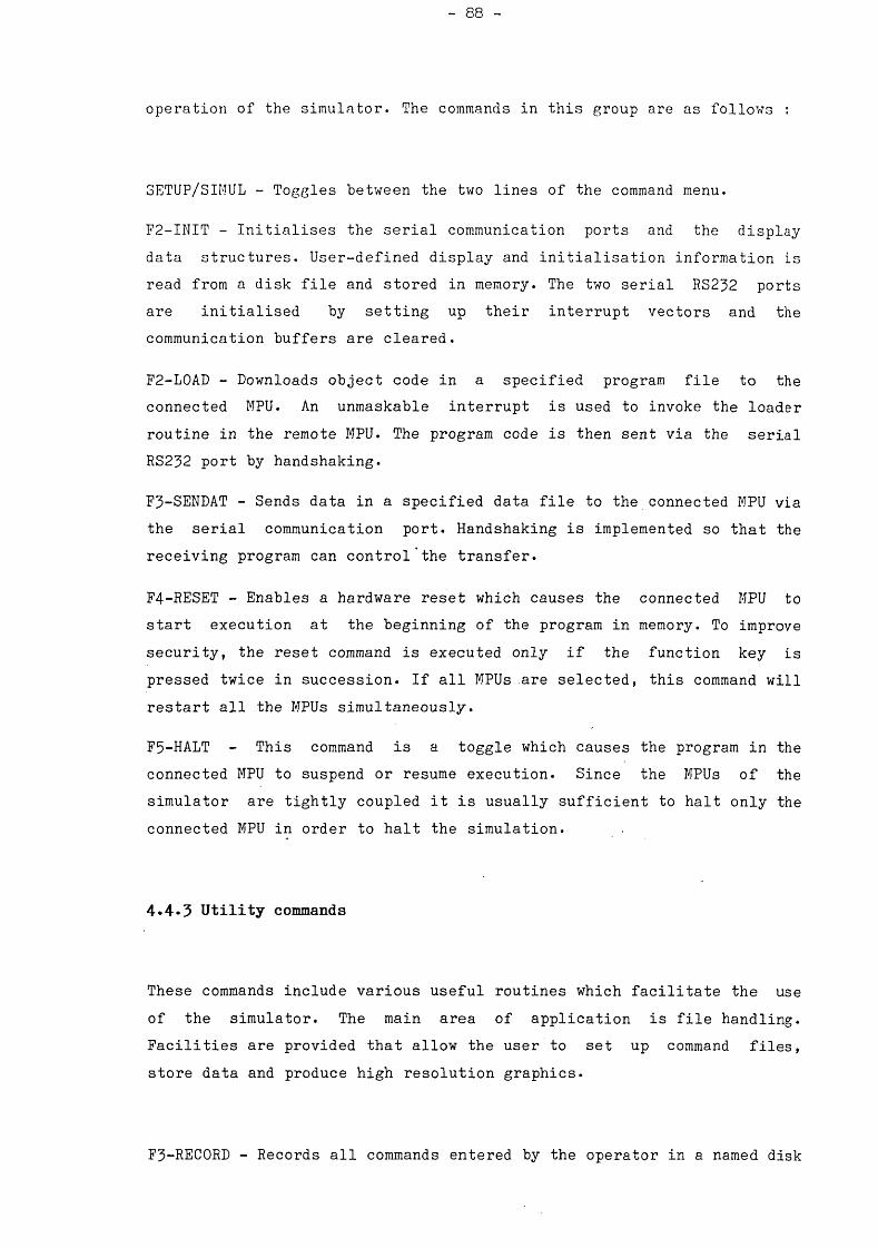
88
operation of the simulator. The commands in this group are as follows :
3ETUP/SIMUL - Toggles between the two lines of the command menu.
F2-INIT - Initialises the serial communication ports and the display data structures. User-defined display and initialisation information is read from a disk file and stored in memory. The two serial RS232 ports are initialised by setting up their interrupt vectors and the communication buffers are cleared.
F2-L0AD - Downloads object code in a specified program file to the connected MPU. An unmaskable interrupt is used to invoke the loader routine in the remote MPU. The program code is then sent via the serial RS232 port by handshaking.
F3-SENDAT - Sends data in a specified data file to the connected MPU via the serial communication port. Handshaking is implemented so that the receiving program can control the transfer.
F4-RESET - Enables a hardware reset which causes the connected MPU to start execution at the beginning of the program in memory. To improve security, the reset command is executed only if the function key is pressed twice in succession. If all MPUs .are selected, this command will restart all the MPUs simultaneously.
F5-HALT - This command is a toggle which causes the program in the connected MPU to suspend or resume execution. Since the MPUs of the simulator are tightly coupled it is usually sufficient to halt only the connected MPU in order to halt the simulation.
4.4-3 Utility commands
These commands include various useful routines which facilitate the use of the simulator. The main area of application is file handling. Facilities are provided that allow the user to set up command files, store data and produce high resolution graphics.
F3-REC0RD - Records all commands entered by the operator in a named disk

- 89 -
file. The system clock is reset and a background task is started which stores all keyed entries and the time on file.
F4-PL0T - Directs incoming data to a graphics terminal. The data is output through a serial port by an interrupt-driven background task.
F5-ST0RE - Stores incoming data as text on a named disk file. The incoming data is received by an interrupt-driven background task.
F6-STATUS - Displays the status of the system or a selected MPU. The function keys are reconfigured such that they can be used to specify the MPU whose status is to be displayed.
F7-CMDFIL - Reads and executes commands stored in a named disk file. A background task reads the commands and passes them to the- command interpreter for execution at the scheduled time. The task terminates at the end of the file or when the command CMDFIL is encountered. Command files can be created by recording operator actions or by editting.
F8-SH0W - Displays the contents of a specified file on the VDU. This command invokes a foreground task whilst monitoring of the MPUs continues in the background. A new menu of commands is displayed and the user can then display any desired page of the file. The commands available under this utility are as follows:
F1-NEXTPF2-PREVPF3-MARKF4-RETURNF5-T0PF6-MIDDLEF7-B0TT0MF8-EXIT
Displays the next page of the file. Displays the previous page of the file. Marks the current page.Returns to a MARKed page.Displays the first page of the file. Displays the middle page of the file. Displays the last page of the file. Exits from this utility.
4 .4 . 4 Interactive commands
This group of commands enable the user to interact dynamically with the simulator.
F6-M0NIT Connects the communication port to a specified MPU for

- 90 -
monitoring and interaction. The function keys are relabelled with user-defined names to indicate the MPUs available for selection. On selecting an MPU, the appropriate display page is written on the screen. When a previously monitored MPU is reselected, old data is displayed in low intensity. New incoming data is written in high intensity.
F7-M0DIFY - To send new values of a variable to the user program in the connected MPU. The function keys are relabelled with user-defined names to indicate the modifiable variables. On selecting a variable, the user is prompted to enter its new value.
F8-EVENT - To send the parameters of an event to the user program in the connected MPU. The function keys are relabelled with user-defined names which indicate the events available for selection. On selecting an event, the user is prompted to enter its parameters.
4-5 PROGRAMMING AND RUNNING INTERACTIVE SIMULATIONS
4 .5-1 Interfacing simulation programs for interaction
Asynchronous communication is implemented between the parallel MPUs and the host minicomputer by a monitor construct. Including its embedded data, the monitor occupies a total of 650 bytes of memory. Its implementation is similar to that of the distributed monitor for parallel communication and it provides a set of routines which may be called from a simulation program.
An interrupt-driven, full duplex protocol allows commands to be sent from the minicomputer while messages are being received from the MPUs. A schematic of the flow of data during interaction between an MPU and the minicomputer is shown in Fig. 4-5« Bearing in mind the dialogue types identified in Table 4.2, the communication scheme was implemented using the following routines
1. INISIO Initialises the RS252 port, enables interrupts and clears

/
Fig. 4̂ *5 Host/Nultiple-MPU communication scheme
W P

the communication buffers.
2. GETVAR - Gets any newly modified variable that has been received from the host. An example of the use of GETVAR is
GETVAR (newvars, stat) ;where newvars is an array of variables which can be modified by the operator.
3. GETEVT - Gets messages scheduling an EVENT that has been specified by the operator. EVENTS are defined as commands from the operator that require specific action in PASCAL. Thus an EVENT would cause the execution of procedures that would not normally be executed. The following is an example of the use of GETEVT to check for a new EVENT and take appropriate action.
GETEVT (evtnum,evt,stat) ;IF stat >= 0 THEN
CASE evtnum OF1 : ApplyFault (evt[l],evt[2],evt[3j);2 : OpenBranch (evt[l],evtf2]) ;5 : ChangeTap (evt[1],evt[2])OTHERWISE SpuriousEvent (evtnum,evt)
END;
4. SNDMSG/PROMPT - Sends a message to the minicomputer for display. A call to this procedure requires the display line to be specified. For example
SNDMSG (length,line,buffer)would send the message in the buffer for display on the specified line. Negative line numbers are defined as ALARMS and specify the display from the bottom of the display page. Furthermore, if the MPU is not connected when the call is made, the message is kept until the MPU is selected. A line number specified as zero is defined as a PROMPT. PROMPTS are sent by polling and a reply is awaited by polling. All other messages are sent by interrupts and a call to SNDMSG only initiates transmission.
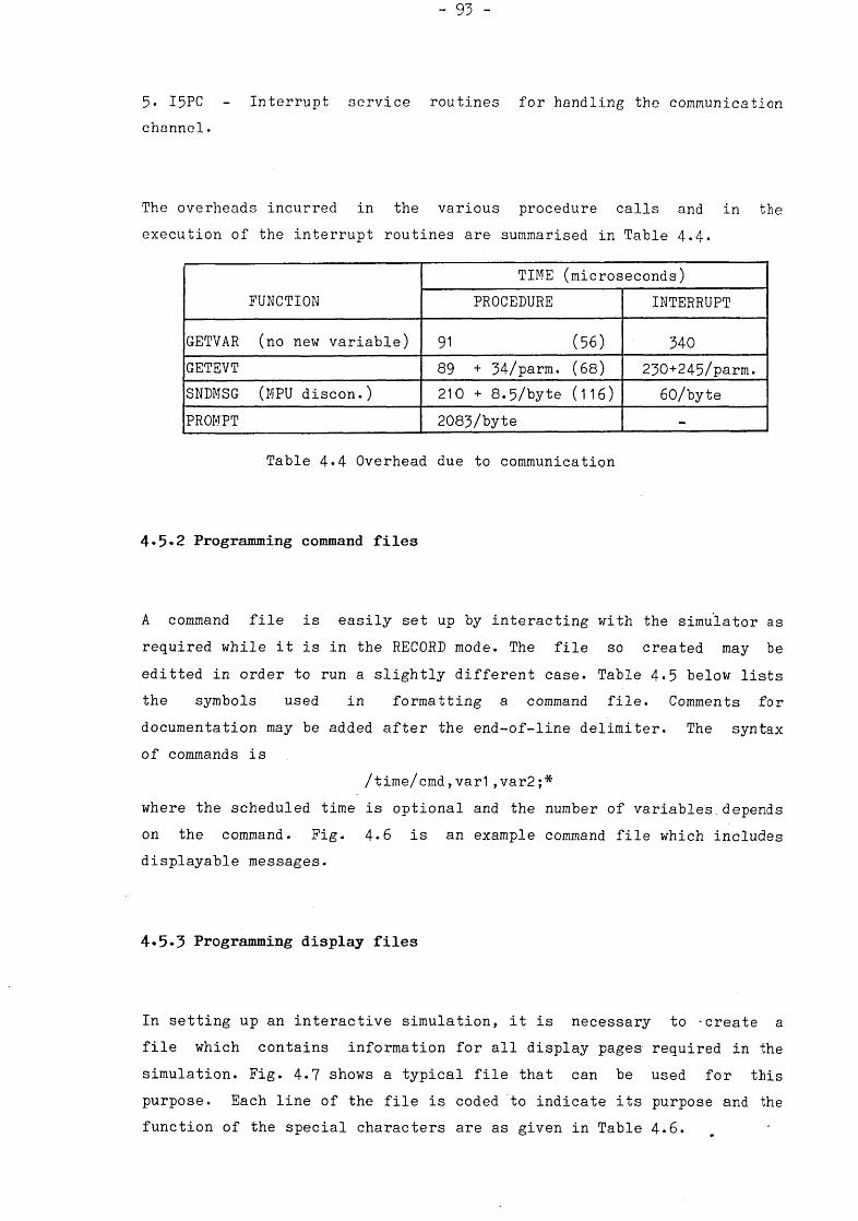
- 93 -
5* I5PC - Interrupt service routines for handling the communication channel.
The overheads incurred in the various procedure calls and in the execution of the interrupt routines are summarised in Table 4.4.
FUNCTIONTIME (microseconds)
PROCEDURE INTERRUPT
GETVAR (no new variable) 91 (56) 340GETEVT 89 + 34/parm. (68) 230+245/parm.SNDMSG (MPU discon.) 210 + 8.5/byte (116) 60/bytePROMPT 2083/byte -
Table 4.4 Overhead due to communication
4»5«2 Programming command files
A command file is easily set up by interacting with the simulator as required while it is in the RECORD mode. The file so created may be editted in order to run a slightly different case. Table 4.5 below lists the symbols used in formatting a command file. Comments for documentation may be added after the end-of-line delimiter. The syntax of commands is
/time/cmd,var1,var2;*where the scheduled time is optional and the number of variables.depends on the command. Fig. 4.6 is an example command file which includes displayable messages.
4«5»3 Programming display files
In setting up an interactive simulation, it is necessary to -create a file which contains information for all display pages required in the simulation. Fig. 4.7 shows a typical file that can be used for this purpose. Each line of the file is coded to indicate its purpose and the function of the special characters are as given in Table 4*6.

94 -
Table 4*5 : List of symbols used in command files
SYMBOL MEANING
$ Message to be displayed on Line 22.T Restart the internal timer.J Variable separator
/ Scheduled time delimiterJ End of command delimiter* End of line delimiterJ End of file delimiterX(Y) Enter SETUP (SIMUL) mode.
$ INITIALISATION OF SIMULATOR */00.00.10/X,2,DSC2:SIMUL/DIS;* ( Enter SETUP mode; initialise |$ SIMULATION PROGRAMS NOW LOADING *f
iSelect and load all MFUs Load program of network MPU
f Send data to network MPUi Send data to generator MPUs *
Y; 6; 6; 2,DSC2:GENPROG;*6; 2; 2,DSC 2:NETPROG;*$ DATA BEING SENT *3,:NETDAT;*6;1;3,:GENDAT1;6;4;3,:GENDAT2;*$ SIMULATION STARTS NOWT* {/00.30.00/6;2;8;1,1,1;* j$ THREE PHASE FAULT OF 80 msec DURATION APPLIED TO BUS 29 * /OO.40.00/8;2,4,29,0,0.08;* i Apply fault to BUS 29/05.00.00/1;* | Go into SETUP mode and end$ SIMULATION ENDS. CONTROL RETURNED TO USER *: I End of command file
Reset timer to zero Select generator models
Fig. 4.6 Example of a command file.
Table 4.6 List of symbols used in display files
SYMBOL MEANING
$ Statement to be displayedT Space allocation for results+ Menu for events& Menu for modifiable variables/ Event prompt* End of display page delimiter» End of line delimiter: End of file delimiter

- 95 -
SAMPLE DISPLAY SETUP FILE
$ SIMULATOR STATUS;$ ----------------------- ;$;$ BACKGROUND COMMANDS;t CMDFIL RECORD STORE PLOT 1;T FILENAME 8;$;t GEN #1 NETWORK GEN #2 GEN #3 LOADS ALL 1;t PROG 9; t DATA 9;S;t DISPLAY FILE : 2;$;$ CONNECTED MICRO STATUS;f HALTED RUNNING INACTIVE 1;$;T CURRENT TIME : 2;+F1-GEN#1 F2-AREA#1 F3-AREA#2 F4-GEN#2 INACTIVE ;*; j End of SYSTEM "block )
$ STATUS OF GENERATORS IN AREA NO. 1;$;$ GENERATOR PARAMETERS;$GENERATOR ANGLE FREQUENCY ELEC. MW MECH. MW AVR VOLT; tUNITI 9;TUNIT2 9;TUNIT3 9;TUNIT4 9;TUNIT5 9;$; 'T ANGLES 9;T MESSAGE:- 8;$;T SIMULATION TIME : 2;
$ UNIT 1 UNIT 2 UNIT 3 UNIT 4 UNIT 5 ;T 9;&F1-DISCON F2-REC0N F3-FASTV F4-AVREF F5-SCH.POW ; j events j +F1-SCALE ; j modifiers J/1 ENTER UNIT ID FOR DISCONNECTION;/1 ENTER UNIT ID FOR RECONNECTION;/2 UNIT ID (0=FAST CLOSE)/(1=FAST OPEN);/2 UNIT ID NEW AVR REF ;/2 UNIT ID NEW SCHEDULED POWER;/ l THIS EVENT IS NOT DEFINED;*; j End of GENERATION AREA NO. 1 block ): | End of file }
Fig. 4.7 Example of a display file.

The overall structure of the display file is such that the first display page is assumed to be the simulator system page. Subsequent pages specify the display information for the MPUs.
4.5*4 Operation of the interactive control program
In order to run interactive simulations it is necessary to produce applications programs which include all the required control and data stuctures for interaction. A text file defining the status display pages of all MPU's being used in the simulation is created as specified above.
Loading and executing the interactive control program results in the user being prompted to select the mode of operation (Normal, Delayed or Single-step). The system page of the simulator and menu (SETUP) are then displayed. The user is now in the interactive environment and may use the function keys to select commands from the menu displayed.
Normally, the first action is to use F2-INIT to initialise the interactive program and load the display information. If desired the session can be recorded by using F3-REC0RD and specifying the file name for storing subsequent commands. Alternatively, if a previously recorded or editted command file is available, F7-CMDFIL can be used to execute the command sequence on it.
The MPUs may be loaded with their respective programs and data by use of the MONIT, LOAD and SENDAT commands. Due to the slow disk access, this process takes about 10 minutes for typical simulations using four MPUs. Faster loading may be achieved if a particular program is to be loaded into more than one MPU by selecting all MPUs and loading them simultaneously with the same program. The other programs may then be directed to the relevant MPUs by using the above sequence.
Execution starts when the MPUs have been loaded with their programs and data. Any MPU may be selected for monitoring by using the MONIT key. The

display is immediately rewritten (in 50 milliseconds) and a link established with the selected MPU. The user may then interact with that MPU by scheduling events or changing the values of variables.
4.6 CONCLUSIONS
Role models of the part man may play in interactive systems have been ■used to define the levels at which interaction may occur. In addition to the requirements of the analyst, consideration has been given to the need for dynamic control required by an operator. It is proposed that the increasing need for educating power system operators should be satisfied by designing systems which can give explicit instructions.
By identifying a set of basic dialogue types, a comprehensive set of procedures was written which may be used to fulfil the requirements of interactive applications.
Two major shortcomings of the interactive environment described are :
1) System portability - the interactive .routines are not portable due to the machine-dependence of the I/O handling. Assembly language had to be used in several areas but the modular techniques, used would simplify implementation on other machines. The need for portable interactive systems may be met by the use of a standard operating system (e.g. UNIX [20]) and handling I/O as logical devices . (for example, see Pfaff et al. [57] on the draft ISO standard Graphical Kernel System (GKS)).
2) Database facilities - the limited capacity and slow access times of the floppy disk system discourage any attempt to provide database facilities. A high-capacity, high-speed hard disk would be required for the implementation of such features.

- 98 -
CHAPTER 5
POWER SYSTEM MODELS AND SIMULATION TECHNIQUES
5.1 INTRODUCTION
Conceptually, a power system comprises electric power sources (generators) and sinks (loads) and the interconnections between them (transmission network). Its normal or intended mode of operation is a steady state in which the power generated matches exactly the load demand plus the transmission network losses. Features which characterise the system include,
a) its large size, both in terms of the number of components and the geographical area it occupies,
b) its sparse interconnection structure,
c) the non-linear behaviour of its components and
d) the wide range of time scales over which its dynamics are manifested.
Stability studies are concerned with the dynamic processes which describe the response of the system to disturbances or operational changes. Although all the components exhibit dynamic behaviour, the time-scale of interest normally allows considerable simplifications to be made in formulating a mathematical model.
Stability studies are normally referred to as short-term, mid-term or long-term as an indication of the time-scales of interest (discussion in Converti et al. [58], Stott [59] )• The studies herein are concerned with the dynamics that occur in the short/mid-term. The models exclude the very fast phenomena such as electro-magnetic transients in the network reactive and capacitive elements, and the very slow changes charac
- 99 -
terising the response of the boilers.
The models used for dynamic stability simulations are presented in this Chapter. A mathematical model of the composite system is then formulated as a set of algebraic and differential equations which describe the time-varying behaviour of its components and their interconnections. Finally, suitable numerical algorithms for the solution of these equations on a digital computer are discussed.
5.2 THE INTERCONNECTING NETWORK
5.2.1 Network models for stability analysis
The model of a power system network for a dynamic stability study is similar to that used for load flow studies but several simplifying assumptions may be made without significant error (Dommel and Sato [3l])* The interconnected transmission .system is modelled as a lumped linear, passive network by making the following assumptions :
1) the network elements may be represented by lumped equivalent elements with constant parameters,
2) the response of the network variables to changes in the loads and generators is instantaneous,
3) the three-phase network is symmetrical and balanced.
The relationship between the bus voltages and currents is given by the matrix equation
[x] - M bus[v] (5.1a)or
[v] - [z]bus[l] (5.1b)
where [Y]-j3US and are the bus admittance and impedance matricesrespectively. As a result of the assumptions listed above the matrix is symmetric when phase shifting transformers are not modelled.

100
Should these be required, efficient methods exist to account for their effect (Dommel and Sato [j5l], Stott [59])*
5.2.2 Data preparation
The base case load flow solution required for the transient stabilitysimulation is prepared by a pre-processing package (Elizarraraz [41])which carries out the following operations :
1 ) Read system data and form the system [y ]-̂ us matrix
2) Order the buses to reduce fill-in during factorisation- using the minimum degree algorithm (Tinney's scheme II [32]).
3) Orientate the network in order to avoid searching for the next element to be eliminated during factorisation.
4) From the M h u s matrix, form the system matrices required for the Fast Decoupled Load Flow (FDLF) algorithm of Stott and Alsac [33] and obtain a load flow solution for the specified operating condition.
5) Form a data file of bus and branch data with the ordering and orientation obtained from steps 2) and 3)* The results of the load flow solution (bus voltages and powers) are also stored in this file.
5*2.3 Network solution
The solution to Eqn. 5*1 may be obtained by inverting the [Y]bus matrix and multiplying by the current vector [i] which is known. Due to the fact that the [z]^us matrix is generally full, it is not calculated explicitly; instead Eqn. 5*1 is expressed as
[1] = [L][u][v] (5.2)
where the lower [l ] and upper [ u ] triangular matrices are obtained by factorising the [Yj-^g matrix. A direct solution of Eqn. 5*2 is easily obtained by forward and backward substi^tion. Since [y ]^us represents an entirely linear network it is only necessary to carry out the factorisation at the beginning of a study. Structural changes during the

101
simulation may be efficiently handled by the use of compensation techniques (Elizarraraz [41], Alsac et al. [60]).
When the factorised [y ]-̂us is being used for the network solution, accuracy is improved by increasing the diagonal dominance of the [y ]-̂ u matrix. This is achieved by representing the loads and generators as Norton current sources and including their shunt admittances in the [Y]bus matrix. Suitable values of these admittances may be obtained from
Yo ■ ( H a - - d V / < B? + Xd - V ( 5 -3 )
where = (Xj + X£)/2
for the generators (Dommel and Sato [3 1]), and
Y0 = S*/V2 (5-4)
for the loads (Arrillaga [61]) -
5-3 GENERATION PLANT MODELS
Fig. 5*1 shows the constituent parts of the generation plant model. It comprises a prime mover which produces a mechanical torque to drive a synchronous generator which in turn produces an electrical torque. These two components are controlled by two main control loops; the excitation loop for voltage control and the governor loop for speed control.
5-3-1 The synchronous generator
The generator model is derived by applying Park’s transformation to the phase variables of a synchronous machine (Adkins and Harley [62], Anderson and Fouad [63])- This results in a 'two-axis' representation with the machine variables and reactances having components along two mutually perpendicular axes stationary with respect to the rotor and referred to as the 'quadrature' and 'direct' axes.

L
Fig. 5.1 Generation plant model

103 -
The particular formulation of the generator model depends on the choice of state variables. Riaz [65] presented equivalent models with flux linkages, currents and a combination of currents and equivalent voltages as state variables. The model used is expressed in terms of stator currents and rotor equivalent voltages. This has the advantage that the machine parameters are in terms of the reactances and time-constants normally measured in tests.
The common assumption that stator transients may be neglected [61-67] is adopted but subtransient effects are included. However, it is assumed that subtransient saliency is negligible. As Dandeno and Kundur have pointed out [66], this means that no special provision has to be made to handle transient saliency.
The complete electrical model of the generator is characterised by the steady-state equivalent circuit diagrams and the block diagram given in Fig. 5*2. It comprises four rotor circuits; a field and a damper winding on the direct axis, and two damper circuits on the quadrature axis. This is equivalent to the Model 2.2 defined by Dandeno and others [64]- A lower order model may be obtained by neglecting subtransient effects (Anderson and Fouad [63]) but the desirability of this simplification is doubtful (Undrill and Laskowski [67]).
The mechanical behaviour of the rotor is represented in terms of its speed and angle. The damping coeffient, D, is used to account for turbine damping only, since the machine damper circuits and the variation of load with frequency are fully modelled (see Ref. [67]).
5»3»2 Excitation subsystem
This subsystem basically consists of an exciter which supplies the field current, an automatic voltage regulator (AVR) for control of the generator terminal voltage, and a stabilising circuit. An IEEE Tyje 1 excitation system model is used (see Fig. 5«3)*
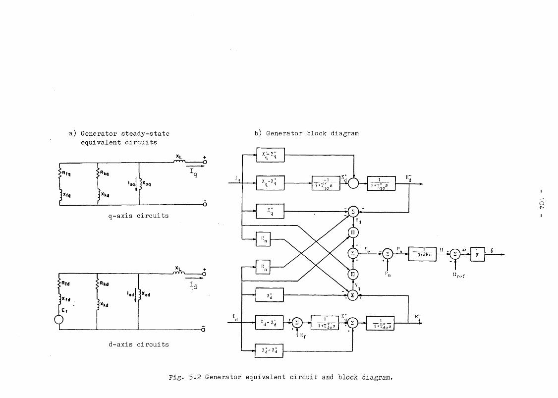
a) Generator steady-state equivalent circuits
q-axis circuits
*L
b) Generator block diagram
i
Fig. 5.2 Generator equivalent circuit and block diagram.
tot

Power system stabiliser Exciter
i
a) Standard model representation
b) Model with redefined state variables
F i g . 5»3 Excitation subsystem model
105

106
Modern excitation systems have a high initial response which may "be detrimental to stability (DeMello and Concordia [68]). This has made it necessary to use supplementary stabilising signals derived from measurable variables such as power output or rotor speed. These signals are added as inputs to the excitation system through a power system stabiliser (PSS). A model of the PSS (IEEE [69]) is given in Fig. 5*3*
The lead-lag circuits present in the standard models have been replaced by first-order lag circuits (Fig. 5«3b). This is a redefinition of the state variables which not only simplifies the application of integration methods (Arrillaga [6l]), but also allows time-constants to be readily associated with each state (Kokotovic et al. [70]).
5»3«3 Speed governor and turbine models
The rotor speed of the generator may be controlled by the action of the governor. In large systems where the frequency is unaffected by changes in one machine, governor action serves to control the power output of the generator. Power is scheduled by varying the governor set-point as shown in the model of Fig. 5*4. Although the governing system may not have a significant effect on first swing stability, its effect on subsequent behaviour may be appreciable (Concordia [71]) *
Fig. 5*4 includes the block diagram of a steam turbine model with provision for control of the intercept or bypass valves as suggested by Anderson (see discussion of Ref. [72]). The model represents a tandem compound steam turbine with a single reheater.
5.4 LOAD REPRESENTATION
The correct representation of load behaviour, both in . its static variation with bus voltage and frequency, and its dynamic response to

CjJ
Fig. 5-4 Governor-turbine model
/
'107

108
sudden disturbances, is now regarded as one of the more important research topics in power systems [74-82]. Conventional stability programs usually represent loads as constant admittances. This is convenient since those admittances may be included in the [y ] ^ matrix and the network reduced to generator buses only.
The significant effect different load models may have on the results of a stability study has instigated research on realistic models which may be easily included in simulation programs. One method is to use second order polynomials which represent combinations of constant power, constant current and constant admittance bus loads (Kent et al. [73])• An exponential representation is simpler to apply and equally effective (discussion of [73]) and this method has been recommended by the IEEE Working Group on the computer analysis of power systems [74]. The authors of a recent EPRI report [75] used high order polynomials In deriving load models from tests but this was primarily due to the statistical method used for analysis.
5»4«1 Static load representation
•An exponential function is used to represent the variation of real and reactive load powers with bus voltage and frequency. This model is valid for bulk supply points where it may be assumed that a load at one bus does not interact with loads at other buses due to the relatively high impedances between them at the sub-transmission or distribution level. The models are expressed by the equations
P = P0 VPvwP“ (5.5)
Q - Q0 V<JV (5.6)
where the exponents pv,pu,qv and q» are referred to as the real or reactive regulation coefficients with respect to voltage or frequency (Venikov [76]). These coefficients may be estimated from test data or from published data for various typical load classes ([75,77])*

109 -
Experience has shown that the performance of these models is unsatisfactory when large voltage excursions occur. This is usually manifested numerically by the failure of the dynamic load flow to converge. Concordia [77] and Kimbark (discussion of [73]) recommended that the model be modified to that of a constant impedance when the bus voltage drops below a critical value (typically 0.7 pu). The authors of the an EPRI report [75] identified this technique as simulating the stalling of motor loads. Venikov [76] also observed that the regulating coefficients vary with voltage but no typical figures were given.
Care must be exercised when modifying the load model to constant impedance in order to avoid a discontinuous change in power. This can be done by calculating the real and reactive powers from
where Pc r i t = PQ Vo r i Pv- 2 ( 5 . 7 )
where Qorit = Qq Vori^V'2 (5-8)
During solution the load current is calculated from Eqns. 5.5-5.6 or Eqns. 5«7-5*8 depending on the voltage magnitude. Recursive solutions for Eqns. 5*5-5.8 are derived in Ch. 6.
P = P ..Vpv"2 cnt
Q = Q ..V^-2 ̂ ^cnt
5«4-2 Dynamic load representation
Individual dynamic loads may be modelled in stability studies if they are large enough to affect the results or when it is their stability that is being studied. The most widely modelled dynamic load in this respect is the induction motor. Its model is derived along similar lines to the generator model. However, its electrical variables are expressed in a reference frame which is chosen to correspond to the synchronously rotating frame of the network. Fig. 5*5a gives the equivalent circuit of an induction motor.
The model is valid for a single-cage induction motor with stator transients neglected. Two state variables represent the electrical dynamic behaviour and the mechanical behaviour is represented by the

110
a) Induction motor steady-state equivalent circuit
Busbar
b) General composite load model
Fig. 5.5 Static and dynamic load models.

anvariation of the rotor slip. The mechanical torque is modelled as exponential function of the rotor speed with the exponent ranging from 0, for paper mills, to 2 for centrifugal pumps.
If motor starting is to be simulated, more detailed modelling of the rotor (inclusion of subtransient effects) is required to represent deep-bar effects or double cage machines (Arrillaga [61], Adkins and Harley [62]).
5.4-3 Composite bus loads
Recent attempts have been made to derive simple models (with one to three time-constants) which may be used to represent composite loads and their dynamics as observed in tests. Chen [75] and Shackshaft [78] have derived such models which include both static and dynamic elements as well as saturation characteristics. Berg [79] and Handschin [80] have proposed methods for aggregating the more readily available data of loads at the distribution level. These methods may be used to derive transmission bus load models which account for the effect of the sub-transmission and distribution networks.
Iliceto and others [81] derived equivalent motor loads for industrial areas by combining parameters of individual motors using statistical techniques. Sabir and Lee [82] used identification methods to derive similar parameters for the representation of paper mill and mining loads. The data available from such studies may be used to implement a general dynamic/static load model as shown in Fig. 5*5b. The constituent parts are totally decoupled and hence may be solved separately. The model is subject to bus voltage and frequency and its solution produces current injections.

5-5 FORMULATION OF THE COMPOSITE SYSTEM MODEL
5-5-1 The composite generation plant model
The models given in Sections 5-2 - 5-4 above represent the behaviour of the individual components. The complete characterisation of the generation plant is easily obtained by connecting the appropriate outputs to inputs according to the plant block diagram (Fig. 5-1 )• The resulting system equation can be written as
_x = [a ]x + _f (_x,_u) (5-9)
y = g(x,_u) (5-10)
with inputs _u, and outputs y;, defined as stator voltages and currents respectively.
The structure of the linear system matrix [a ] (Fig. 5-6) is almost lower block triangular (LBT) due to the sequential nature of the component interconnections. The blocks representing the individual components are lower triangular (LT) with the exception of the exciter which has an internal feed-back loop. The non-linear parts of the system are contained in the vector function f(x,u).
The full model of the power generating plant comprises 17 differential equations plus a few algebraic equations. The differential equations represent the dynamics of the machine, its controls and the prime-mover, whereas the algebraic equations represent the interconnections between the various components. The resulting composite system model is valid for studies extending up to 10-15 seconds after a major disturbance.
5-5-2 Interfacing dynamic components to the network
The complete system model requires the formulation of the equations which describe the interface between the components and the network

swingequations
d-axis
q-axis
excitationsystem
PSS
governor
steamturbine
05
AEd
so_k's2sr
-PhP-I s *
in
XX X X X
— —
XX X
—>< —
ou mpiimc
— - X. —X X 1!
—X X 11
XX
X
X X
-- —
X X X X X X— — —
—- - - XX X
X— -
XX — ■
X X
IN P U rPS-. . . . . . . . . .
—
—
XX X
— -
X X
— - - . . . -- — X XX 1*
[a ]
Fif. 5*6 Generation plant model matrix
• “ - —i
GJ XJ k_EkEdEd
X
XXX
EpRf
'Vr + XvsoVs1vs2Vsr XCy%>
k Eplp
—L J
x + f(x,u)
i
i

114
equations. The interface between the network and an induction motor load is straightforward since the motor model was derived with its electrical variables in a synchronously rotating reference frame which is chosen to correspond to the network frame of reference.
In the case of the generator whose reference frame is fixed to its rotor, a transformation is required to express its variables in the network reference frame. The generator voltages (Vd ,V ) are related to the real and imaginary components of voltage (V^,Vr) in the network frame of reference by
►a ____
l
cos & sinS
_ v -sin 8 cos S
or Vdq = [t ]v .l j m where
where is the instantaneous value offrames. The same transformation matrix [
[T]-1 = [T]T
(5.11a)
(5.11b)
currents to the network currents.
5.6 NUMERICAL INTEGRATION METHODS
Conventional integration methods are generally classed as implicit or explicit depending on whether or not only past values are required to compute new values of the state variables. Methods are referred to as single-step or multi-step depending on the number of past values required. Of the many integration methods available, only relatively few have found applications in power system computation.
5*6.1 Characterisation of integration methods
The analysis of integration methods is usually carried out by use of the scalar test equation

115 -
(5.12a)
with solution x(t+h) = exp(Xh)x(t) (5 .121)where 1 / \ may be regarded as the time-constant of the variation of x. When X is negative Eqn. 5*12 represents an exponential decay and the behaviour is said to be stable. In comparing the performance of different algorithms, the following properties are defined (e.g. see
a) Local truncation error - the error incurred by a method over one integration step.
b) Global error - the error accumulated by a method over an arbitrary number of integration steps.
c) Stability - a method is stable for a given step length if it produces a stable solution to a stable problem; a method which is stable for any step length is said to be A-stable.
d) Convergence - a method which can be made arbitrarily accurate by a sufficient reduction in step length is convergent.
Other properties which affect the efficiency of digital computer implementations, of integration algorithms include :
a) the number of function evaluations required per step,
b) the number of past values that must be stored, and
c) whether or not a system of algebraic equations must be solved at each step.
Ultimately, the efficiency of a method depends on the amount of computer time and (to a lesser extent) storage required to solve a system of ODEs over a given interval to a prescribed accuracy.
5*6.2 Explicit methods
This class of methods may be divided into two sub-classes namely, the Runge-Kutta (R-K) methods and the multi-step methods. Examples of the
Gear [29] for more rigorous definitions).

latter are the Adams-Bashforth (A-B) methods. The Euler method is the simplest method possible and it may be regarded as the first order R-K method or the single-step A-B method (Gear [29])*
Explicit methods now find restricted application in power systems due to their inferior stability properties. In addition kth-order R-K methods require k function evaluations per step whereas k-step A-B methods require information from k previous steps to be stored. Nevertheless, the fourth order R-K method is used in some of the older stability programs (e.g. Dandeno and Kundur [66]) and the simplicity of the Euler method encourages its use for well-behaved problems when neither efficiency nor accuracy is at a premium (Elder and Metcalfe [83]).
5*6.3 Implicit methods
These methods require the solution of a set of implicit algebraic equation at each step. They are normally programmed as the corrector in a Predictor-Corrector (P-C) algorithm where an explicit method is used to predict new values and an implicit method is used to correct those values by iteration. When the iterative process is carried to convergence, the algorithm's properties are those of the corrector method.
Humpage and others [84] have evaluated these methods for power systems problems and found them superior to R-K methods. The improvement was mainly due to the longer step lengths that were possible. Gear [29] derived a class of methods with even better stability properties and therefore efficient for stiff systems. A comparison of the stability boundaries of Adams-Moulton methods (Humpage [84]) with those of the Gear methods indicates the improvement (Fig. 5»7).
In general, the oscillations of the fast states in a stiff system die out after the initial transient. Knowledge of this fact has motivated the use of variable step P-C methods which adjust the step length as well the order of the method to satisfy an error criterion (e.g. VISTA [30]). Hence the expense of small steps is avoided by changing step
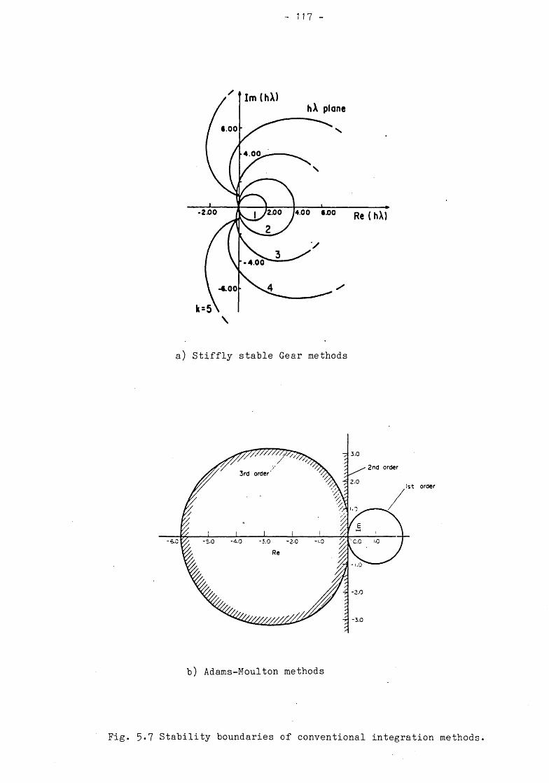
- 117 -
a) Stiffly stable Gear methods
b) Adams-Moulton methods
order
Fig. 5*7 Stability boundaries of conventional integration methods.
sizes when an error criterion indicates the absence of fast varyingcomponents in the solution.
The Backward Euler (B-E) method is the simplest implicit method but its use is limited since the Trapezoidal rule gives superior results for the same amount of work (EPRI [85])* However it is used in variable-step, variable-order codes since it is the first order method of both the Gear and the A-M classes of methods.
The Trapezoidal rule (TR) is a second order implicit method which has gained wide popularity due to its ability to use time-steps larger than the smallest time-constants in a set of equations. Although it has been used quite extensively as the corrector in P-C methods (e.g. second order Adams-Moulton), recent interest has been in major gains attainable in power system simulation by using it to convert the ODEs into algebraic equations which are then combined with the network equations and solved simultaneously [31,58,85]*
Several workers now believe it to he the best method . for power system simulation [59,61,85]* Its main advantage is its stability when solving stiff systems. In common with all implicit methods, it requires a set of algebraic equations to be solved at each step. However, this is not a disadvantage if an iterative solution is required for other reasons. Any algorithm may be used to solve the algebraic equations but in general the Newton-Raphson method is the best (Seinfeld et al. [86]). When the system is linear it converges in a single iteration and non-linear systems converge quadratically. Observing that the equations are usually not iterated to convergence, De Micheli and Sangiovanni-Vincentelli [87] investigated the effect of using a fixed number of iterations.
5*6*4 State transition matrix
A general linear system of ordinary differential equations (ODEs) is represented by the equation

(5 .13 )_x = [a ]x + [b ]uand its solution at a given time t = (n+1 )h is given "by
t[exp([A](r-t))[B]u|dr (5.14)
where exp([A]h) is known as the state transition matrix (STM). This solution is exact once the convolution integral has been evaluated for a specific input function _u. At least one production program has made use of this form (Converti et al. [58]) but, although they calculated the STMs of individual components only, the well known difficulties involved in the calculation of STMs (Moler and Van Loan [88]) have restricted the appeal of the method.
m+1 = exp([A]h)~ n + j
5-7 A TUNABLE INTEGRATION METHOD
In their research into methods for stiff systems of ODEs, Liniger and Willoughby of IBM [89] proposed integration methods with free parameters which could be tuned to suit the eigen-structure of the system of ODEs. The first order method of this class is
xn+1 = xn + h(('-W)xn+1 + win^ (5.15)
where w is a tuning parameter. By using arguments based on digital signal processing techniques, Smith [90] derived a similar formula
xn+1 = xn + sh(vxn+1 + (1-v)*n) (5-16)
where v may be regarded as representing the phase-shift and s the gain. Adopting his recommendation of setting the gain to 1.0 for linear systems and a redefinition of the phase-shift parameter results in Eqn. 5-15-
5-7-1 Comparison with classical methods
Smith [90] pointed out that for specific values of the parameter w, the tunable algorithm (Eqn. 5*15) is identical to classical methods. Some members of the one-parameter family are compared in Table 5*1
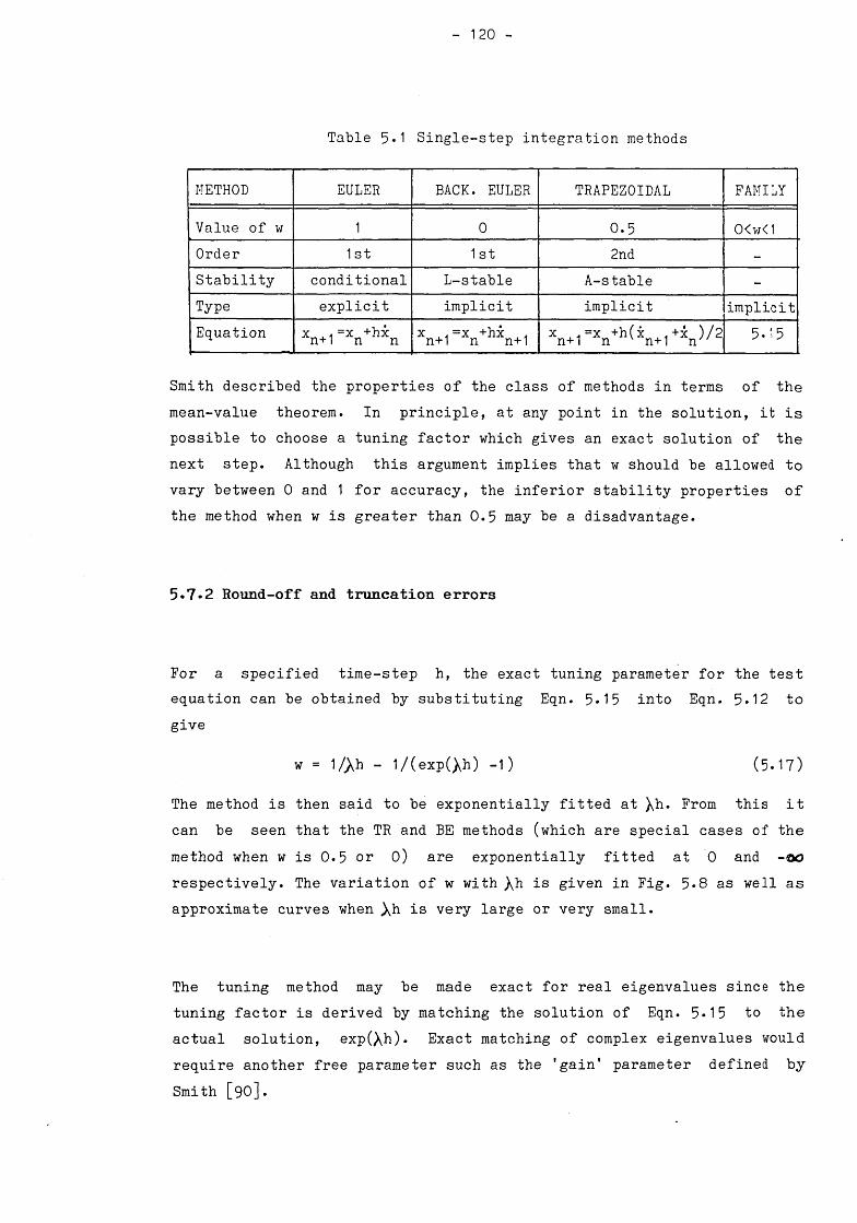
120
Table 5*1 Single-step integration methods
METHOD EULER BACK. EULER TRAPEZOIDAL FAMILY
Value of w 1 0 0.5 0<w< 1Order 1 st 1 st 2nd -Stability conditional L-stable A-stable -Type explicit implicit implicit implicitEquation xn+r V hin x . =x +hx , . n+1 n n+1 x .=x +h(x ,.+x )/2 n+1 n v n+1 n' 5.15
Smith described the properties of the class of methods in terms of the mean-value theorem. In principle, at any point in the solution, it is possible to choose a tuning factor which gives an exact solution of the next step. Although this argument implies that w should be allowed to vary between 0 and 1 for accuracy, the inferior stability properties of the method when w is greater than 0.5 may be a disadvantage.
5<.7-2 Round-off and truncation errors
For a specified time-step h, the exact tuning parameter for the test equation can be obtained by substituting Eqn. 5«15 into Eqn. 5*12 to give
w = 1/>h - 1/(exp(>h) -1) (5.17)
The method is then said to be exponentially fitted at \ h . From this it can be seen that the TR and BE methods (which are special cases of the method when w is 0.5 or 0) are exponentially fitted at 0 and -oo respectively. The variation of w with X*1 is given in Fig. 5*8 as well as approximate curves when Xh is very large or very small.
The tuning method may be made exact for real eigenvalues since the tuning factor is derived by matching the solution of Eqn. 5*15 to the actual solution, exp(Xh). Exact matching of complex eigenvalues would require another free parameter such as the 'gain' parameter defined by Smith [90].

F a
c t
o r
h A ( r e a l p a r t ) - - >Fig. 5.8 Variation of tuning parameter with h\

As an indication of the performance of the method, the test equation 5-12, was solved with different tuning factors. In Fig. 5*9> curves of the accumulated error after 4 seconds are plotted as the time-step, h, is varied. Curves A-E give the error when fixed values of w between 0 and 1 were used; for curve F the appropriate tuning factor for each time-step was used. For large time-steps, the curves show the behaviour of the truncation error and it can be seen that curve F is exact (i.e zero truncation error) subject to the floating-point precision of the Texas FS990/4 computer.
The slopes of the right-hand parts of the curves exhibit the fact that the TR (w=0.5) is a second order method whereas other values of w result in first order methods. However they exhibit lower errors than the Euler (w=1.0). When the method is tuned for the time-step in use, the concept of order loses meaning and this indicates potential' difficulties if on-line error estimation is attempted (Brandon [91>92]).
For very small time-steps, round-off error becomes dominant. The curves indicate that the round-off error of the computer floating-point software is proportional to the number of operations for this example.
A consideration when using any tunable technique is the effect of approximate tuning factors. Fig. 5*10 shows how the accumulated error varies with the tuning factor for different time steps. The general shape is a gradual reduction in error as the optimum tuning factor is approached either from w=0 or w=1. The minimum obtained for values of w greater than 0.5 is due to fortunate cancellation (its position changes with computers of different round-off error). There is considerable variation in the neighbourhood of the optimum point and a very sharp minimum is obtained as the error drops zero. The curves indicate that very accurate estimates of the local time-constants would be required to achieve the highest accuracy, but moderate gains (about an order of magnitude) may be realised if w can be estimated to within _+0.025.

Rela
tive
er
ror
at
T =
4a
Fig. 5.9 Behaviour of global error
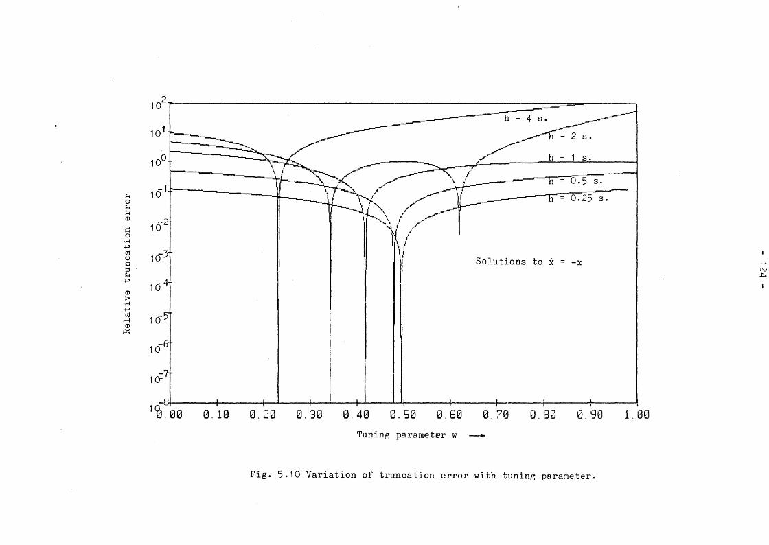
Relative t
runc
atio
n error
Fig. 5.10 Variation of truncation error with tuning parameter.

125
5.7*3 Stability properties
A useful requirement when integrating stiff equations is that of A-stability [29]* For the tunable method the required condition is
xn+1 (1 + wH\)
xn (1 - (1 -w )h\)
which reduces to w <= 0.5 than
When w is less^half, Eqn. 5*15 describes a one parameter family of A-stable methods. Liniger and Willoughby [89] also showed that the method is accurate for these values and defined this property as intermediacy.
A-stability as defined above concerns the behaviour of roots in the left-half complex plane only. It guarantees a stable numerical simulation of an . asymptotically stable system irrespective of the time-step used (Gear [29])* In defining the class of stiffly-stable methods, Gear relaxed this requirement by specifying separate regions for stability and accuracy (see Fig. 5*7). However the first and second order methods are not only A-stable, but their stability regions also extend to the right-half plane. For such methods, the ratio (xn+l/xn) approaches zero as hX -> -oo and the solution is said to be infinitely damped. Methods which exhibit this property are described as L-stable, a definition attributed to Axellson (see Watanabe and Himmelblau [93] or Watts [94]). From Eqn. 5*18, it can be seen that for the TR (w=0.5), (xn+i/xn) — > (-l)n and hence the oscillatory behaviour of large roots.
The stability boundary of the tunable method may obtained by plotting the equality condition of Eqn. 5.18 on the complex hX plane. Eqn. 5*18 may be written as
{a—1/(1-2w)}2 + b2 = {1/(1-2w)}2 (5.19)
where X*1 = a+jb
which describes a circle in the complex plane of radius ( 1 / ( 1 - 2 w ) and centred at (1/(1-2w ) on the real axis. The stability boundaries for

126
various tuning factors (values of w between 0 and 1) are given in Fig. 5*11* When w<0.5 the methods are L-stable and for w>0.5, conditionally stable methods result; at w=0.5 we get the TR which is strictly A-stable.
5.7 .4 Trajectory errors
The selection of integration methods for power systems dynamics has largely been a process of trial-and-error. The difference in the applicability of algorithms to a class of problems may be explained in terms of the position of the dominant eigenvalues in the complex plane. For example, it is well known that the higher order methods of Gear are unsuitable for lightly damped, high frequency components. Similarly, the TR is known to introduce oscillations into the highly damped states of stiff systems (this has motivated ideas of filtering its output (Seinfeld et al. [86])).
In order to determine the type of errors that may be introduced in the trajectory of a solution, Watanabe and Himmelblau [93] proposed a graphical technique for determining the effect of a method on the eigenvalues of a system. Application of the technique results in a chart which shows how the complex plane is transformed by a specific integration method. Interpretation is aided by plotting the chart in terms of the damping ratio f and natural frequency corresponding to an eigenvalue. Thus it can be easily determined whether the calculated trajectory will be more or less damped, or have a higher or lower frequency of oscillation.
Figs. 5.12a-d are taken from [93] and show the trajectory error diagrams for various methods. Fig. 5*12a is for the Euler method and it depicts the mapping of eigenvalues from the left-half plane unto the right-half plane (e.g. A and A') thus causing instability. The stability boundary of the method can be constructed by plotting the original position of roots which are transformed to the imaginary axis. In Fig. 5*12b, both the dominant and extraneous roots (e.g. A' and A") produced by the 2nd order Gear method are indicated.

(A-stable)
Fig. 5*11 Stability boundaries of tunable integration methods
127

1 28
l.C
a) Forward Euler
C
b) Gear (second order)
* ;
c) Backward Euler d) Trapezoidal rule
Fig. 5*12 Trajectory error diagrams of conventional methods

- 1 2 9 -
The trajectory error diagrams of the BE and TR methods (Figs. 5*12c-d) indicate the types of system for which each is suitable. Thus the BE is more appropriate when the roots lie on or near the real axis. The TR, on the other hand, is more suited to oscillatory systems. Purely imaginary roots remain so but with a decrease in frequency; this explains the phase shift observed when this method is used (Anderson and Dembart [95])• Also, large roots that lie near the real axis are simulated with greatly increased frequency (e.g. root A becomes A').
Figs. 5«13a and b, were plotted for the tunable method with w=0.45 and w=0.25* The overall performance is intermediate between the BE and TE._ The curves indicate the improvement that is obtainable over specific regions of the complex plane.
Fig. 5»13c was plotted under the assumption that the real parts of the eigenvalues are known and the tuning factors calculated .accordingly. The much improved fidelity of the representation of the roots is evident. The overall shape of the diagram indicates that the real roots will be accurately simulated whereas imaginary roots (simulated by the TR) will suffer a reduction in frequency. The overall accuracy of a simulation would depend on how accurately the real roots can be estimated and the degree of oscillatory behaviour.
5.8 CONCLUDING REMARKS
A detailed model of a power system has been presented. A 17th order generating plant model is used and the realistic modelling of static and dynamic bus loads has been emphasised. With a linearised transmission network, the resulting composite system model may be expected, to be valid for studies extending up to 10-15 seconds after a major disturbance.
A problem always encountered whenever highly detailed models are used s the availability of valid data. However, Undrill and Laskowski [63] have pointed out that it is usually better to use typical values than reduced

2 .5
2.0
1.5
^r1 .0
0 . 5
01
I
Fig* 5-1'5 Tra jec tory e rr o r difl^rnno o f tunabl« methods

131
models since reduced models may not exhibit certain phenomena even qualitatively. Sensitivity studies of detailed models may then be used to indicate how crucial estimated parameters are to overall performance.
The requirement for accurate simulation of power systems dynamics over an extended time period results in a model that is relatively stiff. The Runge-Kutta algorithm, while accurate, is unsuitable for stiff systems and it has been largely superseded by low order, implicit integration algorithms. Improved numerical integration techniques seem to be among the most promising paths towards high-speed simulations and some investigations using the tunable method are presented in Chapter 6.

132 -
CHAPTER 6
IMPROVED TECHNIQUES FOR DYNAMIC SIMULATION
6.1 INTRODUCTION
At present, most techniques used for dynamic simulation are based on the work of Dommel and Sato [31] who used the Trapezoidal Rule (TR) to discretise the ordinary differential equations (ODEs) of a power system model. The algebraic equations were then either combined with the network equations for simultaneous solution or kept separate and solved in an alternating manner with the network. The effectiveness of the method has been also confirmed by others (Stott [59]> EPRI [85]). Gross and Bergen [96] achieved excellent results by extending the technique to utilise the Gear class of methods. Good accuracy was obtained with the low order methods of the class for full machine models including subtransients.
One distinguishing feature of recent research has been the careful consideration paid to the structure of the power system model. Thus network solution algorithms have been improved by exploiting the almost linear nature of the model and its sparsity [31,32]. For the system dynamics, implicit integration methods have been used to cope with the wide range of time constants [31,59]*
The main aim of the techniques in this Chapter is that of being able to increase integration step lengths without incurring large errors. Vhere possible, suitable approximations are used to speed up the computation without undue loss of accuracy. The ultimate objective is to derive methods which can be used with time-steps that are adequate to represent the dynamics of interest. Ideally, it should be possible to use a single program to produce accurate time plots of both fast and slow variables simply by specifying appropriate time-steps.

153 -
6.2 SIMULATION ALGORITHM
The algorithm developed here was tested on the WSCC standard 9-bus test system [85] shown in Fig. 6.1. The network data and machine parameters used are given in Appendix B. Performance evaluation was carried out for two types of disturbances namely,
a) Outage case - the opening of line 7-5
b) Faulted case - a 3-phase fault on bus 7, cleared by opening line7-5 after 80 milliseconds.
6.2.1 Partitioned solutions
The simulation of a composite power system model requires the simultaneous solution of a large set of ordinary differential equations and algebraic equations. This may be achieved by using an implicit integration algorithm to discretise the differential equations and solving the resultant algebraic equations simultaneously with the network equations with a technique such as the Newton-Raphson.
It is usually more convenient to solve the two types of equations by different methods and this has given rise to partitioned techniques where the network and machine equations are solved separately in an alternating manner. In the general non-linear case, three types of iterations may be required,
a) use of a P-C integration method requires one or more corrector iterations,
b) solution of the network algebraic equations may be carried out by an iterative method such as the Newton-Raphson and,
c) the partitioning of the system gives rise to interface errors which may only be eliminated by iteration.
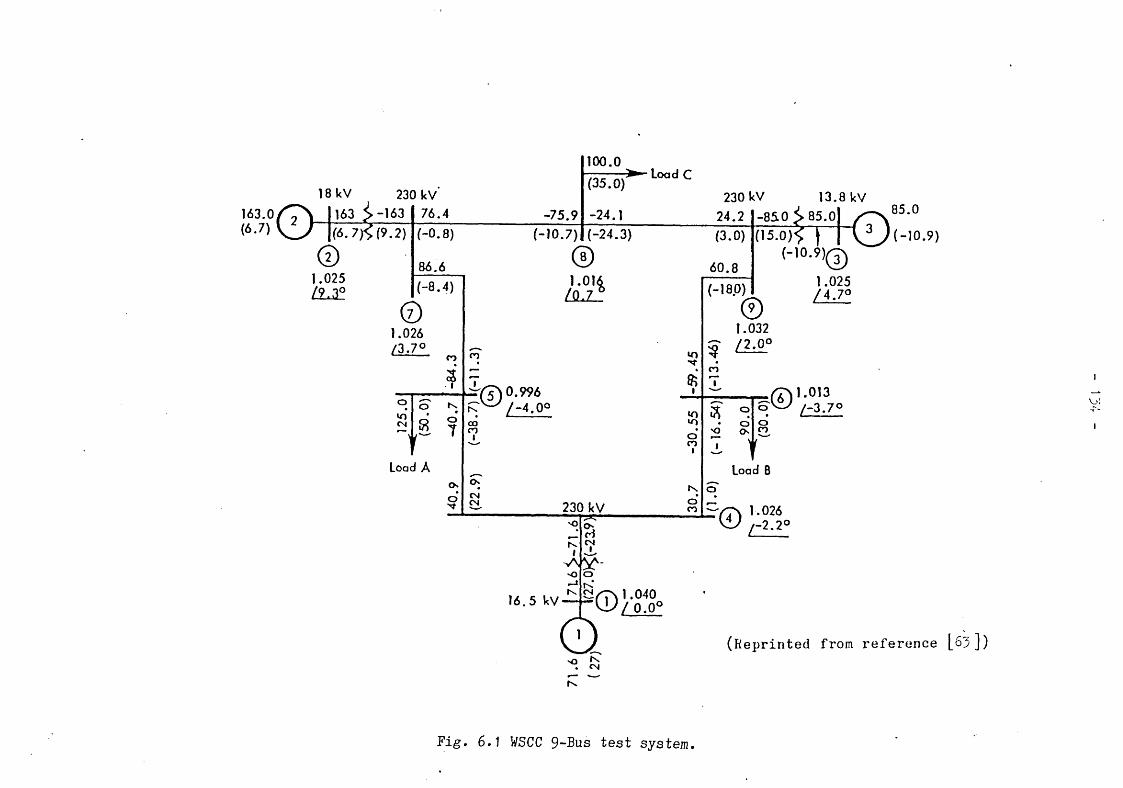
3 . ° / 7 \7 ) v i y
18 kV
163(6.7)
163 j> -163
(6- 7y> (9.2)
230 kV
©1.025
76.4 -75.9(-0.8)
86.6(-8.4)
©1.026/3.7°
r
o
8
Load A
cooSI
Ovo
H O . 7)
100.0
(35.0)
-24.1
Load C
(-24.3)
®1.016
I S L Z 1
CO
±(7 )0 .996/-4.0°
o»CNCM
230 kVo
16.5 kV
CMIVV^A- o —«
230 kV
24.2
13.8 kV
Q<o ^ . CM
<0.1.040/ o . o °
(3.0)
60.8
H8.0)
-850 j> 85.0(150)^ )
( - 1 0 . 9 ) @
85.0
v i ) ( - io.9 )
3
©1.032/ 2.0°
1.025 / 4~7°
*MJI
,(7)1.013 . /-3.7°
TLoad B
( 7 ) 1-026 W ,-2.2°
(Reprinted from reference [63])
F i g . 6.1 W S C C 9-Bus test s y s t e m

135 -
Computational schemes which implement these iterations explicitly are inefficient; it is more efficient to combine them such that at each time-step, the iterations of the machine differential equations are interleaved with those of the network algebraic equations. Interface errors are then automatically eliminated (Stott [59])*
6 . 2 . 2 S o lu tio n o f the swing equation
Gross and Bergen [96] demonstrated the advantage of exploiting the structure of the dynamic stability problem by treating the mechanical and electrical parts of the generators separately. The rotor swing equations are such that an open-loop solution may be obtained. With accelerating power P& as input the rotor speed and angle are given by
w = -7co + <fip 7 = D/2H; <t>= 1/2H (6.1a)
S = « (6.1b)
with being the rotor speed deviation and 7 representing turbine damping. The solution of Eqns. 6.1 is given by
/.t+hco (t+h) = exp (-7h )eo (t) + |^exp[-(t+h-T)7] P (T) dT (6.2a)
A a/•t+h
S ( t+h) = S(t) + co (t )K + - exp[-(t+h-T)7]}Pa(T)/7 dT (6.2b)
where K = [1 - exp(-7h)]//7
In the algorithm of [96], the convolution integrals in Eqns. 6.2 are estimated by numerical quadrature. In that case d(t+h) is calculated explicitly since at the upper limit of the integral in Eqn. 6.2b the multiplicand of P (t+h) is zero. An alternative method is to assume that the variation of P_ over the interval is linearCL
Pa(T) = Pa(t) + h a(t+h)-Pa(t)](T-t)/h t<T<t+h (6.3)
and to evaluate the integral analytically. The resulting expressions are equivalent to the matrix exponent equations derived by Converti and others [58].
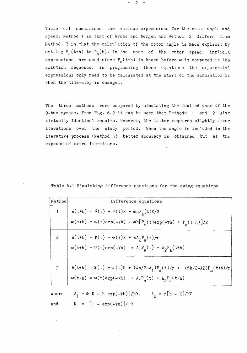
Table 6.1 summarises the various expressions for the rotor angle and speed. Method 1 is that of Gross and Bergen and Method 2 differs from Method 3 in that the calculation of the rotor angle is made explicit by setting Pa(t+h) to P (h). In the case of the rotor speed, implicit expressions are used since P (t+h) is known before o> is computed in the solution sequence. In programming these equations the exponential expressions only need to be calculated at the start of the simulation or when the time-step is changed.
The three methods were compared by simulating the faulted case of the 9-bus system. From Fig. 6.2 it can be seen that Methods 1 and 2 give virtually identical results. However, the latter requires slightly fewer iterations over the study period. When the angle is included in the iterative process (Method 3)> better accuracy is obtained but at the expense of extra iterations.
Table 6.1 Simulating difference equations for the swing equations
Method Difference equations
1 5(t+h) = S(t) + w(t)K + <t>hP (t)K/2Q,
w (t+h) = w(t)exp(-7h) + </>h[P (t)exp(-Th) + P (t+h)]/2a a
2 5(t+h) = $(t) + w(t)K + hA P (t)/yc. 9.
w(t+h) = ̂ (t)exp(-7h) + A.P (t) + A0P (t+h)I Q. c. S.
3 5(t+h) = s(t) +w(t)K + (0h/2-A. )p (t)/y + (<̂ >h/2-A2)P (t+h)/yl a ato(t+h) = w(t)exp(-7h) + A.P (t) + A P (t+h)
I Q. , (i. Q.
where = 4 > [ k - h exp(-7h)]/h7,
and K = [1 - exp(-7h)]/ 7
A2 = </>[h - K]/h7
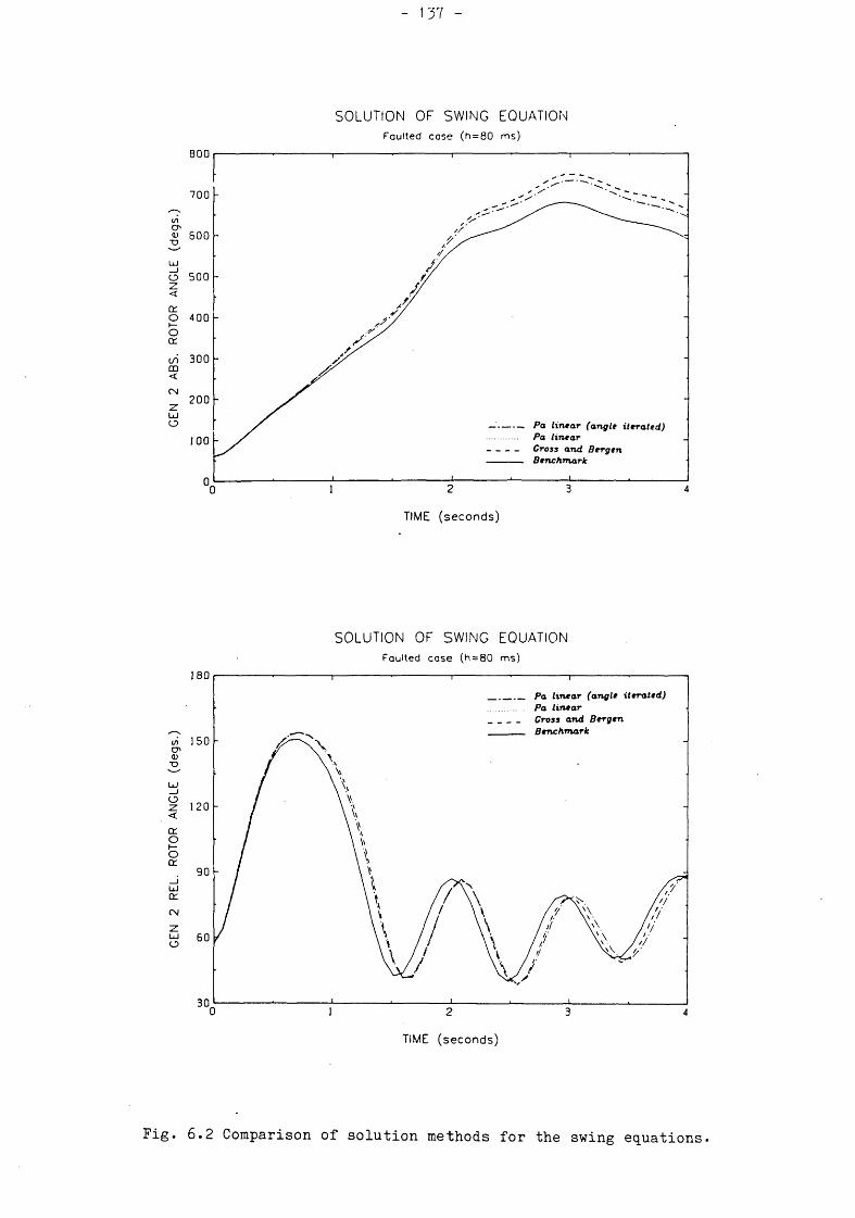
GEN
2
REL
. R
OTO
R
AN
GLE
(d
egs.
) G
EN
2 A
BS.
R
OTO
R
AN
GLE
(d
egs.
)
S O L U T I O N O F S W I N G E Q U A T I O NFaulted cose (h = 80 ms)
S O L U T I O N O F S W I N G E Q U A T I O NFaulted case (h = 80 ms)
Fig. 6.2 Comparison of solution methods for the swing equations.

138 -
6.2.3 Simulation of a generator and its controls
The ODEs representing all dynamic elements in the system need to be converted to difference equations by a discretisation method. The general form of an ODE representing a variable y with time-constant T is
y = -y/T + Kx/T (6.4 )
where the input x may also be a state variable. Discretising Eqn. 6.4 by the TR with a step-length h, gives the difference equation
y(t+h) = y(t) + j-y(t+h)-y(t)+K[x(t+h)+x(t)]}h/2T (6.5a)
which is arranged into the following form suitable for simulation
y(t+h) = F(t) + Gx(t+h) (6.5b)
where F(t) = [(2T-h)*y(t) + h*K*x(t)]/(2T+h) and G = h*K/(2T+h)
Similar difference equations may be written for all ODEs. The sequential nature of the control elements means that when the equations are suitably arranged, they can be solved exactly with the equivalent of one Gauss-Seidal iteration. Thus given the rotor speed deviation, the state variables of the governor-turbine system and the PSS may be obtained in a straightforward manner.
The exciter feedback loop may be handled explicitly by expressing its output in terms of its input signals but this gives rise to dynamic limits which must be calculated and checked at each step [31]• Alternatively an iterative method may be used to solve the matrix block. Such a technique was used but without a separate iterative process since the solution converges in the two or three Gauss-Seidal iterations required by the other equations.
The generator transient and sub-transient voltages on both axes are all coupled via the stator currents. Faster convergence of the iterative algorithm may be achieved by assuming that the stator resistance is negligible. This is equivalent to using the machine short-circuit time constants ([62,63])>

139 -
(6.6a)
(6.6b)
On average, use of this approximation results in one less iteration per integration step.
6 . 2 . 4 Convergence criteria
In principle, the iterative algorithm requires all state variables to be checked for convergence. In power system simulation it is common practice to check only a few key variables instead of a full vector norm [55,85]* The criterion used here requires only a check on the d,q-axis currents and the excitation voltage. The variation in the number of iterations with tolerance is shown in Fig. 6.3 when time-steps of 40 and 80 ms. are used.
Inspection of the time plots in Fig. 6.4 reveals virtually identical results for tolerances up to 0.100. The errors become unacceptable when a tolerance of 1.000 was used with a time-step of 80 ms.
Note that the convergence test does not involve the angle as required by other authors [85] since its calculation is explicit. Even when the calculation of the angle is included in the iterations (Method 3, Table 6.1), a very low tolerance (about 0.001 radian) is required to change the number of iterations significantly.
6.2.5 Solution algorithm
The solution algorithm is similar to that of Gross and Bergen [96] but a partitioned solution is used instead of a simultaneous one. The angle is calculated explicitly with Method 2 of Table 6.1. At the start of each step, the mid-point rule is used as predictor except after switching operations when the Euler formula is used instead.

GEN
2
REL
. R
OTO
R
ANG
LE
(deg
s.)
Ave
rage
N
o.
of
Itera
tions
H O
E F F E C T O F C O N V E R G E N C E T O L E R A N C E
Fig. 6.3 Variation of iterations with convergence tolerance.
C O N V E R G E N C E O F T R A P E Z O I D A L R U L EFoulted case
Fig. 6.4a Effect of convergence tolerance on time response.

GEN 2 REL. ROTOR ANGLE (degs. )
GEN 2 ABS. ROTOR ANGLE (degs:)
141
C O N V E R G E N C E O F T R A P E Z O I D A L R U L E
Fig. 6.4b Effect of convergence tolerance on time response

142
The complete solution algorithm for the power system simulation may be summarised a3 follows
1. Read in data, apply specified disturbance and calculate machine initial conditions from base-case load flow
2. calculate new machine angles using Method 2 of Table 6.13. predict rotor voltages and exciter output4- estimate current injections and solve network equations5. calculate static load demand and integrate dynamic loads6. integrate machine equations to give new voltages7. calculate rotor speed deviation using Method 2 of Table 6.18. solve governor-turbine and excitation system equations9. check stator currents and field voltage for convergence10. if iterations have not converged, go to step 4.11. advance time-step and go to step 2.
The performance of the algorithm was investigated by simulating the two types of disturbances mentioned above. The outage case results in almost linear oscillations whereas the faulted case exhibits large non-linear deviations. This is reflected in the average number of iterations per step given in Table 6.2.
Table 6.2 Effect of time-step on the number of iterations.
No. of iterationsfaulted case outage case
Time-step max . min. avg. max . min. avg.0.010 3 1 1.960 3 1 1 .8180.020 4 2 2.035 3 1 1 .9300.040 4 2 2.090 3 1 2.0100.080 5 2 2.620 4 2 2.1200.120 6 2 3-500 4 2 2.576
Figs. 6.5-6.6 give the time response of the relative rotor angles and electric powers of generator No.2 for both cases. As the time-step is increased the plots exhibit the slight change in frequency of oscillation which is characteristic of the Trapezoidal rule.

GEN
2
REL
. R
OTO
R
ANG
LE
(deg
s.)
GEN
2
AB
S.
ROTO
R
AN
GLE
(d
egs.
)
143
A C C U R A C Y O F T R A P E Z O I D A L R U L EFaulted case
A C C U R A C Y O F T R A P E Z O I D A L R U L EFaulted case
Fig. 6.5 The effect of step length on time response : Faulted case

GEN
2
REL.
R
OTO
R
ANG
LE
GEN
2
AB
S.
RO
TOR
A
NG
LE
(deg
s.)
144 -
A C C U R A C Y O F T R A P E Z O I D A L R U L EOutage cose
Fig. 6.6 The effect of step length on time response : Outage case.

145 -
6.3 TREATMENT OF NONLINEARITIES
The major part of the composite power system model is represented by linear equations. However, some non-linearities are introduced by the presence of nonlinear elements and the interconnection equations. The small number of such equations makes it worthwhile to identify where they occur and to treat them individually. The non-linearities may be classed as either hard (discontinuities) or soft (multiplicative and trancendental functions) and each type requires special techniques.
6.3-1 Discontinuities
The control elements of a power plant contain discontinuous functions such as position and rate limiters. These present problems when any integration algorithm is used. For example, with a P-C method, the algorithm must be restarted at the occurrence of any discontinuity. If the method allows a variable step then the step would be reduced until the discontinuity is traversed with an acceptable error.
The standard manner of dealing with limiters is to set the state to the limited value and its derivative to zero when a limit is reached. Carver [97] and Ellison [98] treated such non-linearities accurately by using interpolation to search for the point where the discontinuity occurred and then integrating up to that point. However the search is expensive due to its iterative nature and the high order formulae used.
The function averaging method of Howe [99] is used here instead. The technique requires the estimation of the integral obtained when the point at which the discontinuity occurs is known. Howe developed the technique for a second order Runge-Kutta algorithm by using an averaged value of the limited state which results in a reduced penalty when a long step is taken across a switching point. For use with the iterative TR algorithm the method may be developed by representing a limiter by the function
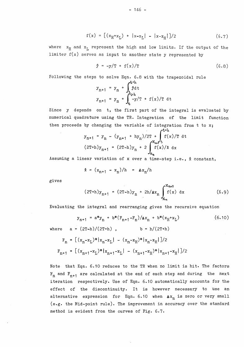
146 -
f(x) = [(xh+xl) + |x-xL| - |x-xh|]/2 (6.7)
where x^ and x^ represent the high and low limits. If the output of the limiter f(x) serves as input to another state y represented by
y = -y/T + f(x)/T (6.8)
Following the steps to solve Eqn. 6.8 with the trapezoidal rule/»t+h
yn+i = y +°n
yn+i = *< + -y/T + f(x )/T dt
on t, the first part of the integralnumerical quadrature using the TR. Integration of the limit functionthen proceeds by changing the variable of integration from t to x;
/•t+Viyn+1 = yn - (yn+1 + hyn)/2T + I f(x)/T at
(2T+h)yn+1 = (2T-h)yn + 2 f(x)/± dx
Assuming a linear variation of x over a time-step i.e., x constant,
x = (xn+1 - xn)/h = Axn/h
gives
(2T+h)yn+i = (2T-h)yn + 2h/ixn dx (6.9)
Evaluating the integral and rearranging gives the recursive equation
yn+1 = a% + b*(Fn*|-Fn)/lxi + b*(xH+xL> (6‘1°)
where a = (2T-h)/(2T+h) , b = h/(2T+h)
Fn = h x n- x L ) * | x n- x L l - (xn - x H) * | x n- x Hl ] / 2
Fn+1 = [ ( xn+1- x L) * | x n+1- x L l - (xn+1- x H) * | x n+1- x Hl ] / 2
Note that Eqn. 6.10 reduces to the TR when no limit is hit. The factors Fn and Fn+ ̂ are calculated at the end of each step and during the next iteration respectively. Use of Eqn. 6.10 automatically accounts for the effect of the discontinuity. It is however necessary to use an alternative expression for Eqn. 6.10 when Axn is zero or very small (e.g. the Mid-point rule). The improvement in accuracy over the standard method is evident from the curves of Fig. 6.7.

GEN 2 REL
. ROTOR ANGLE (de
gs. )
GEN 2 ABS
. ROTOR ANGLE (de
gs. )
147
T R E A T M E N T O F D I S C O N T I N U I T I E S
Fig. 6.7 Treatment of discontinuities

148 -
If the limiter is of the wind-up type (IEEE [69]) no further action is necessary after the iteration has converged. When a print-out of the limited value of x is required an auxiliary variable must be provided. With non-wind-up limiters, the state xn+ ̂ must be limited by application of Eqn. 6.7*
6 .3 * 2 S o lu tio n o f tr ig o n o m e tr ic fu n c tio n s
The transformation between the reference frames of the generators and the network requires the evaluation of the_sines and cosines of the rotor angles at each step. On average, both functions require a total of 26 milliseconds to execute on the TMS9900 processor. This time may be reduced by introducing a pair of ODEs which have S as independent variable. The TR may then be used to derive the difference equations
Provided AS is small at each step, accurate sines and cosines will be obtained. Even in marginally stable cases, the rotors are unlikely to swing through more than 45 degrees during any time-step. This is equivalent to a step length of l/8th of the period of the ODEs which gives good accuracy. Fig. 6.8 shows the effect of this approximation when a long integration step of 80 ms. is used.
Eqns. 6.11 may be programmed to require 1 division and 12 additions and multiplications which, from Appendix A, executes in about 14 milliseconds.
6.3*3 Solution of the load equations
The exponential representation of bus loads is expensive to compute since its evaluation involves PASCAL expressions of the form
where
y.|(S+A8) = Ay, (5) - By2(8) ~ sin(g+A8)
y2(8+A5) = By., (g) + Ay2(S) ~ cos(£+A8)
A = (4-A52)/(4+A82) and B = 448/U+A52)
(6.11a)
(6.11b)

GEN
2
REL
. R
OTO
R
AN
GLE
(d
egs.
) G
EN
2 A
BS.
R
OTO
R
AN
GLE
(d
egs.
)
149
A P P R O X I M A T E S I N E S A N D C O S I N E SFoulted cose (h = 8 0 ms)
A P P R O X I M A T E S I N E S A N D C O S I N E SFaulted cose (h = 80 ms)
Fig. 6.8 Approximate sines and cosines

150 -
P := EXP(k*LN(V))
which may require up to 50 milliseconds to compute (see Appendix A). Considering the voltage dependency of loads as k,
P = P0Vk , P' = k(P/V) where P' = (dP/dV) (6.12)
A common approximation is to assume linearity (Berg [79]) and use
Pn+1 - P J 1 + K V i - Vn ) / Vn l
which is equivalent to Euler integration with respect to V. By using the Trapezoidal rule instead we get the recurrence relation
[2 - k(vn+1 - Vn) A n]pn+1 - ------------------------------------------- Pn ( 6 - H )
[2 - k<Vn+1 - V / V O
which is exact for k=2 and accurate for k between 0 and 3* Eqn. 6.14 requires about 8 milliseconds to execute. A similar expression is used for the load dependence on frequency. A further assumption that the local bus frequency is approximately dS/dt allows us to use
[2 - k(«n+1 - Sn)/Sn]Pn+i - ----------------------- Pn (6.15)
C2 - k<S„+1 - Sn>/Vl1
where & is the load bus angle. These expressions are valid for small changes in voltage and frequency- Thus at the start of the simulation or after switching operations, the Pascal expression above is used.
6-4 APPLICATION OF TUNABLE INTEGRATION
6-4-1 Derivation of difference equations
The difference equations for simulation using the tunable method may be developed in a manner similar to that of Sect. 6.2.3* Discretising Eqn. 6.4 with the tunable integrator and carrying out straightforward manipulations results in the tunable difference equation
■ y(t+h) = F(t) + Gx(t+h) (6.16)

where F(t) = [[(T-hw)y(t) + Khwx(t)]/(T+hv),
G = Khv/(T+hv) and v = 1-w
As for the TR algorithm, the integrating factor F(t) is calculated at the end of each step for use in the next. Recalculation of G is only necessary when the tuning factor or time-step is changed.
6-4.2 Tuning strategies
The options available for choosing the tuning parameters in solving a system of ODEs may be classed as either fixed or adaptive. A further categorisation can be made by specifying whether different parameters are to be associated with each equation or not. Three such categories may be defined as
a) Global - a single parameter for all equations,b) Block - one parameter for each component blockc) Diagonal - one parameter for each individual equation
The various combinations of classes and categories gives a total of six tuning strategies. The fixed tuning methods require a choice of tuning parameters to be used throughout the simulation whereas in the adaptive methods, the parameters are calculated during the solution. The decision as to the number of param'eters rests on considerations of efficiency.
6.4»3 Fixed tuning methods
The use of a fixed global tuning parameter is equivalent to choosing a member of the tunable family of methods. Liniger [lOO] showed that the tuning factor which gives the minimum average discrepancy in approximating all eigenvalues over the whole of the left-half plane is 0.122. This implies that the optimum integration algorithm using Eqn. 6.1 is obtained by tuning at ̂ h=-8.19* In common with classical methods, this choice does not take into account the specific time-step chosen for integration.

Since the roots of any particular system generally occupy specific regions of the complex plane, a prime motivation in using the method is its possible adaptation to suit the eigen-structure of the system. Liniger and Willoughby [89] suggested that the largest eigenvalues of the system should be estimated and the method tuned to their average value. A consequence of this idea is that stiff systems would always be simulated with a small tuning factor and therefore a large stable region on the right-half plane.
The above fixed-global tuning techniques were tested on the 9-bus system by varying the tuning factor over the range 0 to 1. Fig. 6.9 shows the resulting swing curve of generator No. 2 with a time-step of 80 ms. The performance of the algorithm does not change significantly for values of w<0.6. At values approaching 1.0, the effect of any roots outside the stable region is manifested by large errors and a large increase in the number of iterations required per step. No solution could be obtained for values of w greater than 0.8 (see Fig. 6.10).
A fixed global parameter cannot account for the different rates of change of the various states. This may be achieved by using the block or diagonal techniques whose parameters can be chosen by an analysis of the system eigenvalues. However, the computational expense is compounded with the difficulty of associating eigenvalues with individual states and non-linearities which cause the eigenvalues to change with time. A possible alternative is the use of the time-constants of the model to choose a tuning factor for each state variable. This can only be justified for system models in which the states are loosely coupled.
6.4»4 Adaptive tuning methods
Fully adaptive techniques require a calculation of the tuning factors for each state at the end of an integration step. Brandon [91,92] has developed a numerical tuning technique by assuming that each state behaves exponentially at any point in its solution trajectory. A gradient technique was then used to estimate its local time-constant but this required a calculation of the Jacobian at each step.

153
G L O B A L T U N I N GFaulted case
G L O B A L T U N I N GFaulted case
Fig. 6.9 Fixed global tuning

154
FIXED GLOBAL TUNING
TUNING PARAMETER w
Fig. 6.10 Variation of iterations with the tuning parameter.
A simpler method which avoids the calculation of the Jacobian may be developed by assuming that each state varies locally as a first order differential equation with a local time-constant T and a constant inputu
x = -x/T + u (6. 17)
Differentiating with respect to time gives
x = -x/T (6.18)
The local time-constant may then be estimated numerically as
(6.19)
where the 2nd differential is estimated by numerical differentiation. The tuning factors are then calculated from Eqn. 5*11 for use in the next step. After discontinuities or when the value of xR is zero, the tuning factor is set to 0.5* These calculations may be programmed as a single procedure which is called at the end of each step. This is easily incorporated into Step 11 of the algorithm given in Sect. 6.2.
In order to ensure that the method is A-stable other workers [89-92] have limited the maximum value of w to 0.5* As shown in Sect. 5*7.1, an exact solution is possible at each step if the tuning parameters are allowed to vary between 0 and 1. These two alternatives result in A-stable tunable methods and fully tunable methods respectively.
The behaviour of the tuning parameters of some states of the governor and turbine is shown in Fig. 6.11. The oscillatory trajectory of the speed relay gives rise to both positive and negative time-constants (the idea of a negative time-constant is used here to indicate exponential growth). Turning points give rise to sharp peaks as the detected time-constant changes from +oo to -oo. The tuning factor of the reheater state is close to 0.5 which is indicative of its long time-constant.
6.4*5 Evaluation of the method
The tunable methods were tested by simulating the faulted case with

GO
VE
RN
OR
-TU
RB
INE
ST
ATE
S (p
.u.)
FULLY TUNABLE INTEGRATIONFaulted cose (ti=tO ms)
FULLY TUNABLE INTEGRATIONFouited cose (h»4Q ms)
TIME (seconds) TIME (seconds)
FULLY TUNABLE INTEGRATIONFaulted case (h = 1 o ms)
a - sta b le TUNABLE in te g r a tio nFaulted cose (h»40 ms)
TIME (seconds)
Fitf. 6.11 Behaviour of tuning parameters of Governor-Turbine states
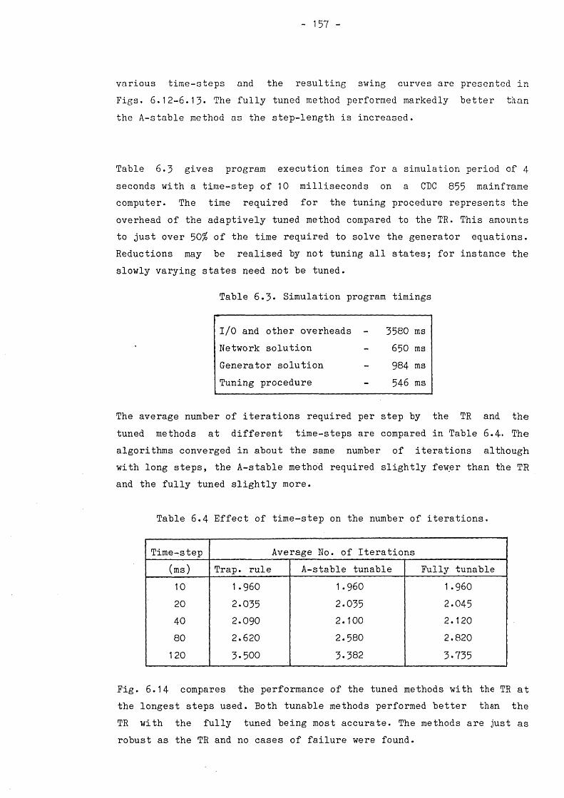
157 -
various time-steps and the resulting swing curves are presented in Fig3. 6.12-6.13* The fully tuned method performed markedly better than the A-stable method as the step-length is increased.
Table 6.3 gives program execution times for a simulation period of 4 seconds with a time-step of 10 milliseconds on a CDC 855 mainframe computer. The time required for the tuning procedure represents the overhead of the adaptively tuned method compared to the TR. This amounts to just over 50$ of the time required to solve the generator equations. Reductions may be realised by not tuning all states; for instance the slowly varying states need not be tuned.
Table 6.3* Simulation program timings
I/O and other overheads 03 o msNetwork solution 650 msGenerator solution 984 msTuning procedure 546 ms
The average number of iterations required per step by the TR and the tuned methods at different time-steps are compared in Table 6.4* The algorithms converged in about the same number of iterations although with long steps, the A-stable method required slightly fewer than the TR and the fully tuned slightly more.
Table 6.4 Effect of time-step on the number of iterations.
Time-step Average No. of Iterations(ms) Trap, rule A-stable tunable Fully tunable10 1.960 1.960 1.96020 2.035 2.035 2.04540 2.090 2.100 2.12080 2.620 2.580 2.820120 3*500 3*382 3*735
Fig. 6.14 compares the performance of the tuned methods with the TR at the longest steps used. Both tunable methods performed better than the TR with the fully tuned being most accurate. The methods are just as robust as the TR and no cases of failure were found.

GEN
2
REL.
R
OTO
R
AN
GLE
(d
egs.
) G
EN
2 A
0S-
RO
TOR
AN
GLE
(d
egs.
)
158
A - S T A B L E T U N A B L E IN T E G R A T I O NFaulted case
A - S T A B L E T U N A B L E I N T E G R A T I O NFaulted cose
Fig. 6.12 The effect of step length on time response : A-stable tuning

GEN
2
REL
. R
OTO
R
AN
GLE
(d
egs.
) G
EN
2 A
BS.
R
OTO
R
AN
GLE
(d
egs.
)
F U L L Y T U N A B L E I N T E G R A T I O NFaulted case
F U L L Y T U N A B L E I N T E G R A T I O NFaulted case
Fig. 6.13 The effect of step length on time response : Full tuning

GEN
2
REL
. R
OTO
R
AN
GLE
(d
egs.
) G
EN
2 A
BS.
R
OTO
R
AN
GLE
(d
egs.
)
T R A P E Z O I D A L Vs T U N A B L E I N T E G R A T I O NFaulted case (h=120 ms)
T R A P E Z O I D A L V s T U N A B L E I N T E G R A T I O NFaulted case (h =120 m s)
Fig. 6.14 Comparative plots of- tuned methods and trapezoidal rule

161
6.5 POWER SYSTEM STABILITY
By definition, power system dynamic stability analyses are carried out to determine whether or not a power system is stable under given perturbations. If we assume that this may be regarded as determining whether the system's eigenvalues have positive real parts, then it is essential that the integration method does not cause eigenvalues to move from the left- to the right-half plane or vice-versa. The first case has been studied extensively because of the attendant numerical instability, but little attention has been paid to the second which may cause an unstable system to appear stable. For this reason (among others), the authors of an EPRI report [85] recommended the use of the TR which is the only linear multistep method that satisfies both requirements. The large stable region on the right-half plane of the BE was regarded as a strong argument against its use for stability studies.
The equations describing the dynamic behaviour of a power system are non-linear and include discontinuities. Any definition of stability in terms of eigenvalues is therefore problematic; e.g. it is unclear whether a system in which a machine slips a pole but subsequently resynchronises is mathematically stable or not. Hence practical definitions in terms of the occurrence of undesirable events such as motor-stalling or pole-slipping are used. It may therefore be argued that determination of the stability of power systems by simulation must rest on the accurate calculation of state trajectories rather than the detection of roots with positive real parts.
The validity of the above argument is illustrated in Fig. 6.15 which shows marginally stable and unstable cases of the 9-bus system with clearing times of 85 and 86 milliseconds respectively. Simulations using the TR and the fully tuned method were performed with one step up to the clearing of the fault and 120 milliseconds thereafter. The TR fails in the stable case whereas the accuracy of the tuned method is maintained. Both methods detect the instability in the second case with the tuned method being more accurate; this may be important when resynchronisation after pole-slipping is being studied.

GEN
2
REL
. R
OTO
R
ANG
LE
(deg
s.)
162
M A R G I N A L L Y S T A B L E C A S EFaulted case ( h ~ 1 2 0 m s)
M A R G I N A L L Y U N S T A B L E C A S EFaulted cose (h=120 ms)
Fig. 6.15 Solution accuracy of marginally stable and unstable cases
6.6 CONCLUSIONS
Numerical methods have been presented which can be used to give rapid simulations of the dynamics of a power system. The methods given for the solution of the swing equations and handling discontinuities are recommended since accuracy is improved at little computational cost.
The use of independent variables other than time has been shown to be a valid manner of treating soft non-linearities. As the simulation progresses and the oscillations die out, the errors introduced by the approximation will be reduced.
Various tunable implicit integration methods have been evaluated by comparison with the Trapezoidal rule. While the fixed tuning methods are easy to implement, they are not recommended since they resulted in no significant improvements. The adaptively tuned techniques performed better and some worthwhile gains were obtained with long time-steps.
As could be predicted from the theory developed in Ch. 5, the fully tunable method was found to be superior to the A-stable technique. We may therefore conclude that restricting the maximum value of the tuning parameters to 0.5 in the interest of stability is neither necessary nor desirable. The fully tuned method is recommended for inclusion in existing programs as an option for use with long steps.

CHAPTER 7
INTERACTIVE DYNAMIC SIMULATION
7.1 INTRODUCTION
The modelling and simulation techniques described in Chs. 5 and 6 are now used to develop a dynamic power system simulator on the parallel processing system of Chs. 2 and 3* The principles of man/machine interfacing discussed in Ch. 4 are applied to develop a flexible interactive system.
The steps to convert a sequential simulation program into a parallel one are outlined and the resulting algorithm is evaluated. The interactive features incorporated into the program are then described. Finally, some illustrative studies are carried out to demonstrate the versatility of the simulator.
7.2 DESCRIPTION OF THE SIMULATION PROGRAM
The dynamic simulation program was developed on the CDC 855 computer and ported to the multiple-processor system. Only minor modifications to the input and output procedures were required to enable the program to run on a single TMS 9900 MPU. The program source code was then partitioned into modules destined for the various MPUs. Finally, the routines for user interaction and interprocessor communication were added.
7*2.1 Program Structure
Fig. 7.1. shows the structure of the complete simulation software. Full

NETWORK MPU
Fig. 7*1 Power system simulator : software structure.

details of the system are given in the user manual [lOl]. The communication and interaction software are as described in Chs. 3 and 4. The application program in each MPU is a Pascal implementation of the dynamic simulation algorithm of Ch. 6.
The features of the Pascal language are fully exploited in the development of the programs. For example, the generator controls are programmed as separately compiled modules in order to facilitate the creation of libraries. Space efficient data structures (Fig. 7.2a) are defined for the generators using of the Pascal facility of variant records. On data input, memory space is allocated as required by the generator model. This allows between 15 and 25 generators to be simulated on a single MPU depending on modelling complexity.
1 * 2 . 2 Partitioned algorithm
In line with the methodology described in Ch. 2, separate modules are defined for the network and rotating machines. The 'star' configuration discussed in Ch. 3 was used. Separate MPUs are assigned to represent the network and rotating machines but the static loads are solved in the network MPU. In order to facilitate the simulation of large systems, more than one machine may be solved on a single processor.
The treatment of dynamic loads maintains the idea of a physical partitioning. In the case of static loads it more important to avoid the transfer of large amounts of data during each step when a non-impedance load representation is used on every bus. This becomes most crucial if an iterative network solution is required. However, when the loads are modelled as composite static/dynamic loads, it is more convenient to solve both parts in the same MPU.
Fig. 7*3 compares the execution sequences of the serial and parallel algorithms for a general system with synchronous generators and induction motors. The parallel algorithm differs from the sequential one in that a minimum of two network solutions are required at each step but

167
GenRec = RECORDJ Generator parameters }
CASE Gov: BOOLEAN OFFALSE : (CASE Exc: BOOLEAN OF
FALSE : ( ) ;TRUE : ({ Exciter parameters j ;
CASE Pss: BOOLEAN OF FALSE : ( ) ;TRUE : (| Stabiliser parameters j))
TRUE : (| Governor-turbine parameters ] ;CASE Exc OF FALSE : ( ) ;TRUE : (| Exciter parameters ) ;
CASE Pss OF FALSE : ( ) ;TRUE : ({ Stabiliser parameters )))
END ;
GenPtr = tGenRec ;
PLANTS = ARRAY [l..Max] OF GenPtr ;
a) Generating plant data structures
Complex = RECORD Re,Im : REAL ENT ;
Message = RECORDSwitched,Converged,Restarted,Stopped : BOOLEAN ; SystemFrequency,SlackAngle : REAL ;Currents for Voltages) : ARRAY [l..Max] OF Complex
END ;
b) Message data structure
Qpointer = tQrecord ;Qrecord = RECORD
Time, Eventnum : INTEGER ;Parameters : ARRAY [1..NJ OF Values ; NextEvt : Qpointer
END ;
c) Event queue data structure
Fig. 7.2 Typical Pascal data structures
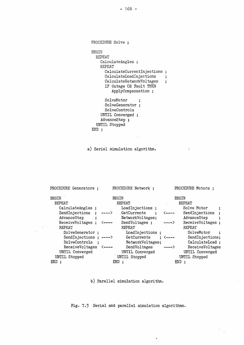
168 -
PROCEDURE Solve ;
BEGINREPEATCalculateAngles ;REPEATCalculateCurrentlnjections CalculateLoadlnjections CalculateNetworkVoltages IF Outage OR Fault THEN
ApplyCompensation ;
SolveMotor ; SolveGenerator ; SolveControls
UNTIL Converged ; AdvanceStep ;
UNTIL Stopped END ;
a) Serial simulation algorithm.
PROCEDURE Generators ; PROCEDURE Network ; PROCEDURE Motors ;
BEGIN BEGIN BEGINREPEAT REPEAT REPEATCalculateAngles ; Loadlnjections ; Solve Motor ;Sendlnjections ; --- > GetCurrents ; <--- Sendlnjections ;AdvanceStep ; NetworkVoltages; AdvanceStep ;ReceiveVoltages ; <--- SendVoltages ; ---> ReceiveVoltages ;REPEAT REPEAT REPEATSolveGenerator ; Loadlnjections ; SolveMotor ;Sendlnjections ; --- > GetCurrents ; <--- Sendlnjections;SolveControls ; NetworkVoltages; CalculateLoad ;ReceiveVoltages <--- SendVoltages ---> ReceiveVoltages
UNTIL Converged UNTIL Converged UNTIL ConvergedUNTIL Stopped UNTIL Stopped UNTIL Stopped
END ; END ; END ;
b) Parallel simulation algorithm.
Fig. 7»3 Serial and parallel simulation algorithms.

- 169 -
this is normally needed for convergence (see Table 6.2). Maximum parallelism is obtained by advancing the time-step after the solution for the rotor angles rather than after convergence of the iterations*
7-2.3 Interprocessor communication
The partitioning technique results in minimal data transfer between processors during the solution. At each step the network and rotating machines exchange terminal voltages and injection currents. Various flags must also be passed between the processors to co-ordinate the solution. A third requirement is data collection for the calculation of global values such as system frequency. In general these data exchanges are required at each time-step and can therefore be grouped into a single message such as that shown in Fig. 7.2b. During each step, the network broadcasts this message to all machines and receives a corresponding message from the machines with the high-level protocols given in CH. 3*
7-2.4 Interface to the interactive control program
Interactive control of the simulator is achieved by the use of the monitor which implements the dialogue types defined in Ch. 4. ¥hen actions must be carried out in a strict sequence (e.g. setting-up the simulation), use is made of the PROMPT primitive to request parameters from the user. Results and messages from the MPUs are sent using SNDMSG. These I/O operations are designed to be compatible with the display pages on the host minicomputer.
Procedures are defined for actions that may be carried out interactively. Where a control action only requires changes to a single variable, that variable is declared as modifiable. All other actions are defined as EVENTS and provision is made to pass their parameters to appropriate procedures (see Sect. 4.5*1)• At each step during the simulation, the procedures GETVAR and GETEVT are used to check for any operator actions.

170 -
7-3 PERFORMANCE TESTS
7«3»1 Test systems
The simulator performance was evaluated by simulating the dynamics of the WSCC 9-bus network of Fig. 6.1, and the IEEE 14-bus and 30-bus systems (see Fig. 7*4). Data for the test networks and generating plant are given in Appendix B. Base-case load flow solutions for the systems were obtained off-line to a tight tolerance of 0.001 p.u. real and reactive power mismatch at each bus. The synchronous compensators of the 14 and 30-bus systems were modelled as generators without prime movers.
7«3»2 S eq u en tia l a lg o rith m
Table 7.1 gives program timings of various routines when the test systems are solved on one MPU. From the timings of the 9-bus system, it can be seen that the CDC 855 mainframe computer (Table 6.3) is about 400 times faster than the TMS 9900 microprocessor when I/O is not considered. The accuracy of solution was compared with that of the mainframe and the effect of round-off error was found to be small.
Table 7.1 Sequential algorithm program timings
RoutineTest system
9-bus 14-bus 30-busms/step ms/step ms/step
Network 510 900 1850Loads 220 720 1330
Angles 180 270 350Generator 130 215 260Controls 450 545 620
Advance step 600 720 830Input/output 1130 1215 1260
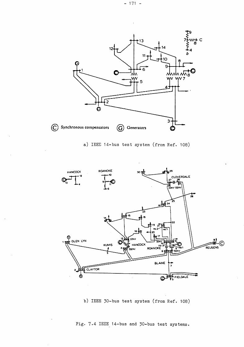
171
a) IEEE 14-bus test system (from Ref. 108)
b) IEEE 30-bus test system (from Ref. 108)
Fig. 7*4 IEEE 14-bus and 30-bus test systems.

7-3*3 Parallel algorithm
Fig. 7-5 shows timing diagrams of the program for the 9-bus system being solved on 2 MPUs when the computation pattern achieves a steady state. A straightforward partitioning of the serial algorithm would result in the execution pattern of Fig. 7.5a. It is evident that the idle time is unnecessarily large due to the time the network MPU spends waiting for data from the generators. Fig. 7.5b shows the improvement obtained when the order of solution is changed to correspond to the parallel algorithm of Sect. 7.2.2.
Table 7.2 Parallel algorithm timings
No. of MPUs
1 2 3 4ms ms eff. ( % ) ms eff• ( % ) ms
9-bus 2860 1670 86 1670 57 1670 43(with I/O) 4800 3260 74 2420 66 1670 72
1 4-bus 4990 3440 73 3360 50 3360 37(with I/O) - 4100 - 3360 - 3360 -
30-bus 8420 6700 63 6700 42 6700 31(with I/O) - 6700 - 6700 - 6700 -
The times for a single step of the parallel algorithm in Table 7.2 indicate that the loss in performance is due primarily to the unequal partitioning resulting from the constraints of the physically-based method. Thus without the printing of results, the execution time of the 9-bus system is that required to solve the network and loads. This is reflected in the low efficiency figures for the parallel solutions. When the generator results are being output incremental improvements are obtained with up to 4 MPUs.
The task of partitioning into roughly equal parts would become less of a problem when large systems are solved on a large number of MPUs since the solution of one component would require a relatively short time.

2460 ns (estimate)-
GENERATOR NETWORK GENERATOR NETWORK
Angles 180 ms Loads 220 ms
’/M M /'.' f/ / / / / ; / 7'/# ! • /
ICalculate
network voltages510 ms
Generator: 130 ms % Loads 220 msSolvecontrols450 ms
n/ / ’///>/ •' ’ >, O// ///,. //,/ / / / ; / / / /j ///TJJTrrrnjTTT'
■///;,■ m //// '/////)//////
Calculate network voltages
510 ms
Advancestep600 ms
V ) ? ;} r rH'7?. / / / / f ///■// /
/ / / f/ /// ////////////
Angles 180 ms Loads 220 ms
Advancestep600 ms
i
Calculate network voltages
510 ms
V
Loads 220 msGenerators 130 ms
Solvecontrols450 ms
ICalculate
network voltages
510 msw /m r m /m v
b) Modified algorithm
a) Simple algorithm
Pig. 7-5 Parallel simulation timing diagrams.

174 -
However, with typical network solution times being about 30% of the total computation (Detig [36]), if the generating plant are to be solved on more than two MPUs then the network solution must be partitioned.
7-4 INTERACTIVE FEATURES
7*4.1 Simulation set-up and control
A simulation session starts with the loading of all the MPUs with their appropriate programs and data. The user is then prompted to select the generation plant model by including or excluding stabiliser, exciter and governor-turbine circuits.
Any member of the one-parameter family of tunable methods (see Ch. 6) may be selected by an appropriate choice of the tuning parameter. Some control over the execution of the algorithm is possible by a choice of the integration time-step, the convergence tolerance and the rate at which output data is to be printed.
7 «4«2 Network sw itch in g and load changes
Network changes are effected by the use of compensation techniques to modify the network solution to account for the changes. Any network change which can be represented by a modification matrix can be easily implemented e.g. multiple outages, transformer tap-changing or node addition and removal (see Alsac et al. [60]). The technique has been extended to handle unbalanced faults (see Elizararraz [41])-
Network branches may be disconnected and previously disconnected branches may be reconnected. Changes in branch admittances are used to simulate the switching of parallel lines. The switching of a line into a system in the steady-state may be simulated by initialising the simulation with that line removed.

175 -
Two methods are used to simulate static load changes. When all loads are represented by impedances, the compensation method is applied to the network solution. With non-impedance loads, changes are accounted for by modifying the load injection currents.
7»4»3 Interaction with generators and motors
Set-points in the generator controls are made adjustable by declaring them as modifiable variables. This also applies to other values that are normally constant but used during every time step. An additional feature is the capability of ramping a variable up or down at a specified rate. This was used to implement turbine fast-valving.
The tripping of a generator is 'simulated by modifying the injection current it sends to the network to the value required to compensate for the admittance included in the [y ]^us matrix. The load rejection performance of the machine may be studied by continuing the solution of its equations. Resynchronisation of the machine can be achieved by advancing its load angle to correspond to that of its terminal busbar. Motor disconnection and reconnection are similar to the same operations on a generator except that when a motor is reconnected it is not necessary to advance its rotor angle.
7 .4 . 4 User interation
Output from the parallel execution units is displayed on the console of the host minicomputer. A separate page was allocated for each MPU and typical examples are shown in Fig. 7*6. The text in bold type is generated by the monitored MPU and displayed at a high intensity. Low intensity text is stored within the host as specified on the display file. The examples show the application of a fault on the network and the modification of a generator set-point with appropriate messages from the MPUs.

POWER SYSTEM DYNAMIC SIMULATOR
STATUS OF NETWORK AREA
BUSBAR VOLTAGESBUS VMAG. ANGLE BUS VMAG. ANGLE BUS VMAG. ANGLE1 0.76 11.10 2 0.71 4.73 3 0.66 -13-254 0.70 -7-77 5 0.70 -5-14 6 0.75 -21.447 0.75 -17.05 8 0.85 -20.88 9 0.74 -18.7910 0.74 -19-56 11 0.74 -20.62 12 0.74 -27-1213 0.73 21.96 14 0.72 -21.24
SIMULATION TIME : 0.080 seconds
MESSAGE 3-PHASE FAULT ON LINE 2 5MESSAGE Line 2 5 disconnected. Fault cleared
TIME TYPE NEARBUS FARBUS DURATION0.0 4 2 5 0.08
F1-MODELS F2-FAULT F3-0UTAGE F4-SHED F5-L0ADS F6-CHANGE F7-M0DIFY F8-EVENT
POWER SYSTEM DYNAMIC SIMULATOR
STATUS OF GENERATORS IN 14-BUS SYSTEM
GENERATOR PARAMETERSUNIT ANGLE FREQ. ELEC. MW MECH. MW AVR VOLT PSS TERMV REL.1 17.29 60.68 10.42 0 2.04 0 1.04 -38.322 24-11 60.81 22.53 0 1.70 0 0.95 31.513 32.11 60.18 5-25 39-55 2.11 0.05 0.96 23-504 22.70 60.59 24.28 0 2.28 0 0.98 32.925 55-62 60.23 173-33 231.96 1.34 0.05 0.96 0PLOTVARS :- 2.04 1.70 2 .11 2.28 1.34MESSAGE :- Unit 3 AYR Ref. changed from 1.05 to 1.10
SIMULATION TIME : 1.20 seconds
UNIT1 UNIT2 UNIT3 UNIT4 UNIT5 Generator bus : 8 3 2 6 1
TIME UNIT No. NEW REFERENCE1.2 3 1.1
F1-DISCON F2-REC0N F3-FASTVF4-AVREFF5-SCH.P0W F6-CHANGE F7-M0DIFYF8-EVENT
Fig. 7.6 Typical simulator display pages
177 -
The interactive facilities described may be used at will by typing in the appropriate commands at the console of the host minicomputer. A feature of the implementation is that it is not necessary to halt the simulation before making any changes. In order to facilitate the execution of complicated command sequences, a first-in-first-out queue (see Fig. 7*2c) was implemented in each application program. This enables a timed sequence of events to be stored in each MPU. At each time-step, the list is checked for any events which are scheduled for execution. The list may be set up, modified or purged on-line.
As described in Ch. 4, simulation sessions may be repeated by recording all commands typed in and running the simulation from the resulting file.
7-4*5 Post-processing
Due to the limitations of the hardware, few post-processing facilities are included in the simulation software. Two features that were regarded as essential are the storage of output data and an on-line graph plotting capability. Use of the STORE command directs incoming data to a disk file whereas PLOT sends data to the graphics display terminal. Any further post-processing must be carried out off-line.
7.5 SIMULATION STUDIES
The versatility of the simulator is now demonstrated by means of some studies that can be conducted. The examples chosen serve to indicate its usefulness as a tool for interactive power system analysis.
7•5-1 Critical fault clearing time
The critical clearing time of any fault may be determined by running simulations with different clearing times. .This exercise is facilitated

178 -
by allowing the user to specify both the post-fault integration step and the number of steps to be taken during the fault. Fig. 7.7 depicts marginally stable cases of the various systems studied.
7»5«2 Pole slipping and re-synchronisation
A remotely connected generator which loses synchronism with the rest of the network would resynchronise after slipping a few poles if the driving torque is suitably reduced by governor action. This mode of operation may be employed if the output of the generator is required to maintain system integrity (Adkins and Harley [62]) and the resulting power pulsations are not detrimental to the rest of the system (Venikov [76]).
Fig. 7*8 shows curves from a simulation of the pole-slipping and resynchronisation process. The machine slips two pole-pairs and then resysnchronises under the action of fast-valving.
7.5.3 Load representation
The effect of non-impedance static load representation on the dynamic behaviour of a power system was investigated with the simulator. The marginally stable case of the 9-bus system was simulated with various load representations. As the representation approaches a constant load demand, the peak angular swing of the faulted generator is reduced. Comparative swing curves are shown in Fig. 7.9*
7.6 CONCLUSIONS
As is well known, the derivation of a parallel algorithm which also results in an efficient partitioning of the computational task is heavily dependent on the architecture of the hardware on which the

179 -•
TIME ( seconds)
Fig. 7*7 Marginally stAble cases
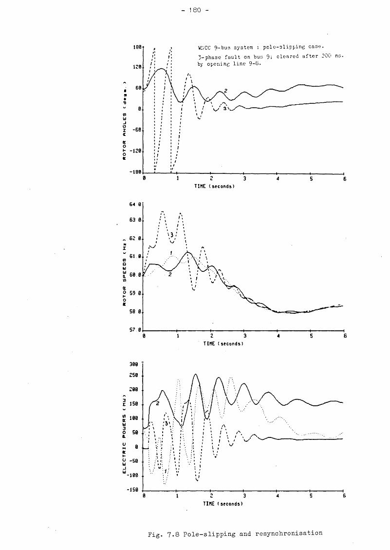
ELEC
TRIC
POW
ERS
(MW)
RO
TOR
SPEE
DS (H
z)
ROTO
R AN
GLES
Cd
«g»
180
TINE (seconds)
TINE ( seconds)
TINE ( seconds)
Fig. 7.8 Pole-slipping and resynchronisation

POU
ERS
( MU
) RE
L. RO
TOR
RNG
UE
( d
e g »
181
TIME (seconds)
pv=2.0
TIME ( seconds)
Fig. 7.9 The effect of load representation.

182
problem is to be solved. The algorithm derived here is general purpose in that it may be used on any multiple processor system. The task decompositon is such that the time for interprocessor communication is insignificant compared to the serial computation between data exchanges. In implementing the algorithm, there is scope to reorder the solution sequence to reduce idle time.
The technique may be easily extended to large networks in which case the solution time will be dominated by the network solution. Since the method of solving the network is largely independent of that used for the rotating machines, parallelism may be exploited in the network solution itself.
In designing the simulator proper consideration has been given to the problems of implementing interative user interfaces* Simulation and modelling techniques have been chosen not only on the basis of their efficiency but also on their suitability for on-line interaction. The system is highly interactive and one of its features is that changes may be made without halting the simulation.

183 -
CHAPTER 8
CONCLUSIONS
8.1 GENERAL
Research into parallel processing techniques continues apace in the computing community. This effort promises highly parallel hardware architectures and the software tools to exploit parallelism. In the meanwhile the techniques investigated in this work can be used with commercially available equipment to achieve worthwhile gains in execution speed for power system simulation problems.
In this final chapter some conclusions are drawn from the experience of designing and implementing a multiple processor simulator. The performance to be expected from presently available equipment is indicated and some suggestions are put forward for the direction of future research.
8.2 HARDWARE AND SOFTWARE
8.2.1 Hardware
The simulator uses the TMS 9900 microprocessor which was announced in 1976. At the time of writing, more powerful processors with 32-bit data paths and address spaces in the megabyte range are common. Architectural enhancements include pipe-lining, on-chip cache memory and hardware support for multi-processing (see Gupta and Toong [102]). Other trends which simplify the implementation of multiple processor systems include the off-loading of specific I/O functions to special-purpose chi.ps and the embedding of common communication protocols in hardware.

184 -
The speed of floating-point arithmetic which was found to determine the execution time of the simulation has been improved by two orders of magnitude by the use of hardware units in the form of co-processors (execution times of the Intel 8087 [106] are given in Appendix A). Thus simulation of the 9-bus system which is 40 times slower than real time may be done faster than real time with new equipment. Problems with round-off error are now unlikely since up to 80 bits may be used to represent a real number.
The architecture of the simulator may be quite expensive when several processors are used since each processor requires a parallel port for every other processor with which it needs to communicate. A more cost-effective solution would make use of a parallel bus system. The bus bandwidth would not have to be very high due to the low communication rate of the method of decomposition. The short message length also eliminates the need for a large common memory since each processor only requires a small message buffer.
8.2.2 Software
Transportability of the present simulator software is assured since the bulk of it is in PASCAL. Although some routines were written in assembly language, the equivalent routines would not require a large programming effort. The exception to this is the software required for interaction. That part of the simulator would have to be rewritten to exploit the particular hardware features of any new equipment. The ease with which this could be done depends, to a large extent, on the type of operating system provided by the equipment supplier.
Although a high degree of standardisation has been achieved in programming languages, the need for transportable operating systems has been recognised only recently. An example of the few available systems is Unix [20]. The possibility thus exists of not only transporting the algorithmic part of a program but also its data processing part. In particular, Unix, which is written in the high-level language C, is an interactive multi-tasking operating system under which concurrent
185
processes may be created and executed. This considerably simplifies the development of interactive interfaces.
A major difficulty encountered in the simulator project was the lack of software tools for developing and debugging parallel programs. Typically correcting an error that requires a recompilation of the network and generator programs takes about an hour. Most of this time is due to the very slow access time of the floppy disks. A hard disk would speed up this process significantly.
The AMPL system was useful for debugging programs on a target system but its design does not allow the debugging of a multiple processor system. A debugger which can be switched between several processors much like the interactive control program is essential to develop parallel processing algorithms.
8.2*3 Interaction
The implementation of interaction was much simplified by the use of the dialogue types identified in Ch. 4* The use of role models of the user's part in an interactive environment eases the task of providing a consistent set of commands. The model of interactive computation derived from these user models provides a general purpose framework for structuring interactive systems. This viewpoint of interaction occupies a higher level o'f abstraction than the graphical kernel system [54] which is primarily concerned with device handling.
The design of the simulator has been geared towards the needs of research and real-time simulation. The provision of command files and event queues simplifies the use of the simulator as a research tool; users may regard the system as a programmable device. Although the detailed models used cannot be simulated in real time, the interactive facilities could be used with simplified models running in real-time.

186
8.3 SIMULATION TECHNIQUES
8.3-1 Model formulation
The partitioned method of formulating the power system model used in this work is based on the physical relationships between the various components of the system. This approach was extended by Talukdar [103] in the METAP simulator and recently formalised by Saeks and Decarlo [104] as the component connection model (CCM). The identity of each component is maintained and a composite system model is formed by means of a connection matrix.
The advantages of this approach include ease of formulation and programming. Libraries of components may be created and adding a new component requires only a modification of the connection matrix. It is also well suited to interactive simulation since changes can be made to parameters with very little overhead.
8 .3 -2 S o lu t io n m ethods
Several new approaches to the solution of the ODEs describing a generating plant have been investigated and found to result in improved performance. The importance of the order of solution of the equations has been explained in terms of the sequential connection of control elements. This allows their solution to be obtained in one Gauss-Seidal iteration.
The method used for treating soft non-linearities is an elementary application of the method of continuations whereby algebraic equations are converted to a differential equations and solved by numerical integration. The effectiveness of the technique is due to an implicit linearisation at each step. Howe’s method for handling discontinuities improves the handling of limiters by making a first order approximation of the point within a time step at which switching occurs.

187
Gear recently identified the need for low-order, low-accuracy, single- step methods which can be used for real-time simulation [107]• The tunable method may meet this need by virtue of its ability to use very long steps. The method can be easily added to existing programs which make use of the Trapezoidal rule. Its use is strongly recommended although further work in the form of an error analysis is required.
8.3«3 Parallel algorithms
The partitioning method used in deriving a parallel algorithm may be regarded as a block partitioning of the composite system matrix. Total solution times are therefore quite long relative to communication time and other overheads. This contrasts with the scheduling algorithm proposed by Brasch et al. [ll] which requires a problem to be decomposed into a set of elementary arithmetic operations.
Although the coarseness of the component-wise decomposition may result in idle time, the large number of components in typical power systems would reduce the effect of unequal partitioning. As shown in Ch. 7, it is also po.ssible to rearrange the order of solution in order to reduce idle time. This allows some flexibility in designing parallel algorithms of the type analysed in Ch.
8.4 ORIGINAL CONTRIBUTIONS
The following are considered by the author to be original contributions to the field of interactive power system computation :
design and implementation of a multiple processor simulator.The simulator comprises a network of interconnected MPUs whose structure can be configured to suit a power system problem. An architecture is proposed which can utilise parallel bus systems.
distributed monitors for interprocessor communication (Ch. 3). Since parallelism is exploited at a macroscopic level, it is

188
possible to utilise the monitor concept for interprocessor synch -ronisation. Recently proposed message-passing primitives are then added to provide communication.
formulation of a model of interactive computation (Ch. 4).A consideration of the roles man may play in an interactive system and the possible modes of interaction led to a model of computation which can be used for designing man/machineinterfaces. Six basic dialogue types are identified from which more complex types can be built.
- analysis and implementation of a tunable integration method.The analysis carried out (Sect. 5*7) indicated that better accuracy would be obtained if the requirement for A-stability is relaxed. The method is equivalent to the Trapezoidal rule when short steps are used but it is superior with very long steps.
treatment of non-linear functions by continuations (Sect. 6.3)* Continuous non-linear functions are converted to ODEs and solved by numerical integration. The method is effective for non-linear functions which may be expensive to compute.
treatment of discontinuities by Howe's method (Sect.By assuming a linear variation of a state variable subject to limits, simple expressions are derived which implicitly estimate the point at which switching occurs. This results in a noticeable improvement in solution accuracy.
8.5 SUGGESTIONS FOR FURTHER WORK
8.5-1 Model reduction
The simulator execution speed may be improved by the use of model reduction techniques. Most such techniques emanating from control theory carry out complex transformations on the states of a linear system model. The requirement for interaction restricts the choice of technique to those that maintain the physical identity of each component. The CCM methodology coupled with the method of singular perturbations (Wasychnuk and Decarlo [105]) seems a promising path to reduced models which retain

189 -
structural identity. Significantly, it seems possible to extend both methods to non-linear systems.
The method of singular perturbations has undergone significant refinement under Kokotovic and co-workers [70] and may be used not only for model reduction but also for time-scale decomposition. This can be used to implement multirate integration algorithms. The asymptotic theory on which the method is based can also be used to estimate the length of time during which highly damped fast states are active. This information can be then used to implement a simulation algorithm with on-line model reduction.
8.5-2 Simulator expansion
A versatile simulator has been developed which can be used for the interactive simulation of power system dynamics as well as other interconnected dynamical networks. While the project has been successful in attaining its original aims, it has also highlighted areas in which further development work needs to be done. The basic design concepts for a simulator have been shown to be flexible enough to be implemented on presently available equipment. This section indicates the areas which need to be considered before acquiring new hardware and software for an upgraded system.
Cost - The cheapest method of development would be to design and build special hardware for the application, but this would require an excessive length of time. The most cost-effective approach is to purchase off-the-shelf systems which may then be configured to suit.
Performance - Due to the rapid rate at which the performance of modern equipment is improving, it is necessary to aim for an adequate standard of performance such that the system is not obsolete by the time the project is completed. In this respect the only criterion to be considered is that of speed. Other aspects, such as ease of use and variety of features available, are mainly dependent on software and can
190 -
therefore evolve with further development.
Development and maintenance - Despite the cost penalty, it would be necessary to purchase a host development system for the initial development work as well as upgrading and modification of the simulator. This is essential in a research environment and it is to be expected that this capability would be desirable in a commercial system as well. It is possible to use cross-support equipment but a native system would be more appropriate. As shown by this project, a host computer can be made into a useful and integral part of the simulator.
Miscellaneous equipment - A wide variety of input/output equipment may be added either as peripherals to the development system or as global resources to be shared by the multiple MPUs. Depending on the application, mass storage (e.g. hard disks), display (e.g. colour graphics) and input devices (e.g. bit-pad) may be required.
8-5-3 Simulator applications
In its present state the simulator can serve as a useful tool for the evaluation of control algorithms. 'In the case where the control is to be applied to a single machine, the generator program can be modified to include the controller; e.g. by replacing the power system stabiliser model. A more complex controller may be implemented on a separate MPU which executes in parallel with the simulator; this only requires the addition of a suitable communication procedure to the generator program.
System-wide control strategies such as automatic generation control or load frequency control may be studied by monitoring all processors. The host computer can be used for this purpose but the existing minicomputer is ill-equipped for this task. A more powerful host computer with a hard disc and graphics support is required. It would then be possible to implement a database and more powerful post-processing facilities.

191
Table A.1 Execution speed of Texas Pascal constructs.
Pascal Execution speedconstruct (microseconds)
FOR loop 310
REPEAT loop 40
WHILE loop 90
CASE statement 530
IF statement 370
Assign constant 160
Assign variable ' 170
Assign element of ARRAY 380
PROCEDURE calls
no parameter 450
value parameter 500
VAR parameter 500
FUNCTION call
one parameter 730
NEW statement 22000
DISPOSE statement 22000
SIGNAL statement 830
WAIT statement 830
Notes : 1 - All constants, variables and parameters are of type integer.
2 - The NEW and DISPOSE statements operated on a recordcomprising an integer and a pointer.
3 - The SIGNAL and WAIT procedures operated on the predefined type SEMAPHORE.

Table A.2 Execution speed of floating-point arithmetic
InstructionExecution speed (microseconds)
INTEL 8086/8087 TEXAS TMS 9900
5 MHz. 3 Mhz.
Add/subtract 14/18 1130/1150
Multiply 18 1150
Divide 39 1850
Square root 36*
24000
Tangent 110 25000
Arctangent ■ - 12000
Sine/cosine - 1 3000
Exponent - 30000*
Logarithm - 25000*
Raise to power 130 -
These values vary over a range of one half to three times depending on input data.
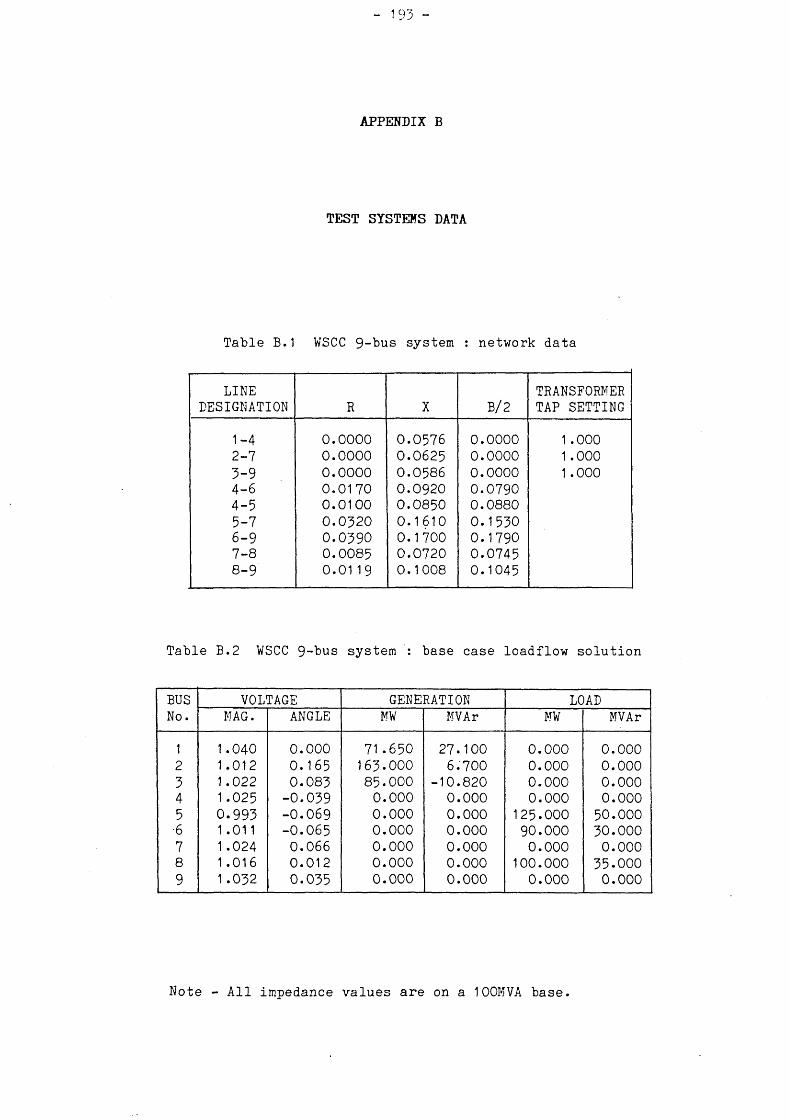
APPENDIX B
TEST SYSTEMS DATA
Table B.1 WSCC 9-bus system : network data
LINEDESIGNATION R X B/2
TRANSFORMER TAP SETTING
1-4 0.0000 0.0576 0.0000 1 .0002-7 0.0000 0.0625 0.0000 1 .0003-9 0.0000 0.0586 0.0000 1 .0004-6 0.0170 0.0920 0.07904-5 0.0100 0.0850 0.08805-7 0.0520 0.1610 0.15306-9 0.0390 0.1700 0.17907-8 0.0085 0.0720 0.07458-9 0.0119 0.1008 0.1045
Table B.2 WSCC 9-bus system : base case loadflow solution
BUS No.
VOLTAGE GENERATION LOADMAG. ANGLE MW MVAr MW MVAr
1 1.040 0.000 71.650 27.100 0.000 0.0002 1.012 0.165 163-000 6.700 0.000 0.0003 1 .022 0.083 85.000 -10.820 0.000 0.0004 1.025 -0.039 0.000 0.000 0.000 0.0005 0.993 -0.069 0.000 0.000 125.000 50.000•6 1.011 -0.065 0.000 0.000 90.000 30.0007 1 .024 0.066 0.000 0.000 0.000 0.0008 1 .016 0.012 0.000 0.000 100.000 35.0009 1.032 0.035 0.000 0.000 0.000 0.000
Note - All impedance values are on a 1OOMVA base

Table B.) IEEE 14-bus system : network data
LINEDESIGNATION R X B/2
TRANSFORMER TAP SETTING
1 -2 0.01938 0.05917 0.02641-5 0.05403 0.22304 0.02462-3 0.04699 0.19797 0.02192-4 0.05811 0.17632 0.01872-5 0.05695 0.17388 0.01703-4 0.06701 0.17103 0.01734-5 0.01335 0.04211 0.00644-7 0.00000 0.20912 0.0000 0.9784-9 0.00000 0.55618 0.0000 0.9695-6 0.00000 0.25202 0.0000 0.9326-11 0.09498 0.19890 0.00006-12 0.12291 0.25581 0.00006-13 0.06615 0.13027 0.00007-8 0.00000 0.17615 0.00007-9 0.00000 0.11001 0.00009-10 0.03181 0.08450 0.00009-14 0.12711 0.27038 0.000010-11 0.08205 0.19207 0.000012-13 0.22092 0.19988 0.000013-14 0.17093 0.34802 0.0000
Shunt capacitor on bus 9 0.1900
Table B.4 IEEE 14-bus system : base case loadflow solution
BUSNo.
VOLTAGE GENERATION LOADMAG. ANGLE MW MVAr MW MVAr
1 1.060 0.000 232. 460 -26.410 0.000 0.0002 1.045 -4.945 40. 000 20.640 21.700 12.7003 1.010 -12.589 0 . 000 13.910 94.200 19.0004 1.034 -10.495 0 . 000 0.000 47.800 -3.9005 1.041 -9.017 0 . 000 0.000 7.600 1.6006 1.030 -15.049 0 . 000 44.350 11.200 7.5007 1.041 -13.899 0 . 000 0.000 0.000 0.0008 1.090 -13*900 0 . 000 30.470 0.000 0.0009 1.027 -15.663 0 .000 0.000 29.500 16.60010 1 .020 -15.865 0 . 000 0.000 9-000 5.80011 1.021 -15.604 0 . 000 0.000 3.500 1 .80012 1 .015 -15.956 0 . 000 0.000 6.100 1.60013 1.011 -16.037 0 .000 0.000 13.500 5.80014 1 .001 -16.895 0 . 000 0.000 14.900 5.000

Table B.5 IEEE 30-bus system : network data
LINEDESIGNATION R X B/2
TRANSFORMER TAP SETTING
1-2 0.0192 0.0575 0.02641-3 0.0452 0.1852 0.02042-4 0.0570 0.1737 0.01843-4 0.0132 0.0379 0.00422-5 0.0472 0.1983 0.02092-6 0.0581 0.1763 0.01874-6 0.0119 0.0414 0.00455-7 0.0460 0.1160 0.01026-7 0.0267 0.0820 0.00856-8 0.0120 0.0420 0.00456-9 0.0000 0.2080 0.0000 0.97806-10 0.0000 0.5560 0.0000 0.96909-11 0.0000 0.2080 0.00009-10 0.0000 0.1100 0.00004-12 0.0000 0.2560 0.0000 0.932012-13 0.0000 0.1400 0.000012-14 0.1231 0.2559 0.000012-15 0.0662 0.1304 0.000012-16 0.0945 0.1987 0.000014-15 0.2210 0.1997 0.000016-17 0.0824 0.1923 0.000015-18 0.1070 0.2185 0.000018-19 0.0639 0.1292 0.000019-20 0.0340 0.0680 0.000010-20 0.0936 0.2090 0.000010-17 0.0324 0.0845 0.000010-21 0.0348 0.0749 0.000010-22 0.0727 0.1499 0.000021-22 0.0116 0.0236 0.000015-23 0.1000 0.2020 0.000022-24 0.1150 0.1790 0.000023-24 0.1320 0.2700 0.000024-25 0.1885 0.3292 0.000025-26 0.2544 0.3800 0.000025-27 0.1093 0.2087 0.000027-28 0.0000 0.3960 0.0000 0.96827-29 0.2198 0.4153 0.000027-30 0.3202 0.6027 0.000029-30 0.2399 0.4533 0.00008-28 0.0636 0.2000 0.02146-28 0.0169 0.0599 0.0065
Shunt capacitors - bus 10 bus 24
0.19000.4300

196 -
Table B.6 IEEE 30-bus system : base case loadflow solution
BUSNo.
VOLTAGE GENERATION LOADMAG. ANGLE MW MVAr MW MVAr
1 1 .060 0.000 261.070 -26.890 0.00 00.002 1.045 -5.507 40.000 44.630 21 .70 12.703 1.033 -8.121 0.000 0.000 2.40 01.204 1.027 -9-795 0.000 0.000 7.60 01.605 1 .010 -14*315 0.000 32.140 94.20 19.006 1.017 -11.430 0.000 0.000 0.00 0.007 1.007 -13.139 0.000 0.000 22.80 10.908 1.010 -12.057 0.000 16.940 30.00 30.009 1.022 -14.924 0.000 0.000 0.00 0.0010 1 .007 -16.750 0.000 0.000 5.80 2.0011 1.082 -14.924 0.000 31.060 0.00 0.0012 1.012 -16.128 0.000 0.000 11.20 7.5013 1.071 -16.128 0.000 45.060 0.00 0.0014 0.997 -17.071 0.000 0.000 6.20 1 .6015 0.993 -17.139 0.000 0.000 8.20 2.5016 1.002 -16.694 0.000 0.000 3.50 1.8017 1.000 -16.959 0.000 0.000 9.00 5.8018 0.985 -17.758 0.000 0.000 3.20 0.9019 0.984 -17.916 0.000 0.000 9.50 3.4020 0.989 -17.688 0.000 0.000 2.20 0.7021 0.993 -17.227 0.000 0.000 17.50 11.2022 0.993 -17.211 0.000 0.000 0.00 0.0023 0.982 -17.487 0.000 0.000 3.20 1 .6024 0.976 -17.573 0.000 0.000 8.70 6.7025 0.966 -16.965 0.000 0.000 0.00 0.0026 0.947 -17.431 0.000 0.000 3.50 2.3027 0.969 -16.304 0.000 0.000 0.00 0.0028 1.013 -12.029 0.000 0.000 0.00 0.0029 0.948 -17.680 0.000 0.000 2.40 0.9030 0.935 -18.671 0.000 0.000 10.60 1 .90

197 -
Table B.7 Rotating machine data
V/SCC 9-bus system units IEEE 30-bus system units
1 2 3 1 2 5,11,13 8
Ra 0.0000 0.0000 0.0000 0.0000 0.0000 0.0000 0.0000Xd 0.8958 1 .3125 0.1416 0.3576 1.4000 2.1660 7.0760Xq 0.8645 1.2578 0.0969 0.3424 1 .3067 1.4400 3.4200X'd 0.1198 0.1813 0.0608 0.0475 0.2467 0.4880 1.2160<•- 1
q 0.1980 0.2300 0.0750 0.0831 0.4800 1.4400 2.3180X"d 0.0890 0.1070 0.0450 0.0364 0.1733 0.3110 0.8040X"q 0.0890 0.1070 0.0450 0.0364 0.1733 0.3110 0.8040T ' do 6.0000 8.9600 5.8900 4.2000 6.1000 6.0000 8.0000T' qo 0.5350 0.4000 0.6000 0.5650 0.3000 0.1500 0.1500T"do 0.0330 0.0250 0.0330 0.0320 0.0380 0.0500 0.0525mT qo 0.0780 0.0500 0.0700 0.0620 0.0990 0.0150 0.0151H 8.0000 23.6400 3.0100 13*6800 4.6400 1.0500 0.3000D 1.0000 1.0000 1.0000 1.8000 1.0000 0.1000 0.0100
Table B.8 Exciter data
WSCCunits
Ka Ta Ke Te Kf Tf Vrmax Vrmin Se
1,2,3 25.00 0.20 -0.0601 0.6758 0.1080 0.350 1 .0 -1 .0 0.226
IEEEunits
1 25.00 0.20 -0.0582 0.6544 0.1050 0.350 1 .0 -1 .0 0.2502 20.00 0.02 1.0000 0.9420 0.0300 1.000 1 .0 -1 .0 0.000
5,11,13 20.00 0.05 -0.1700 1.0000 0.0700 1 .000 1 .0 -1 .0 0.5008 80.00 0.05 -0.1700 0.9500 0.0400 1.000 1.0 -1.0 0.500
Notes : 1 - All data is from Ref. 63«2 - Impedance and inertia values are on a 100 MVA base.3 - The IEEE 30-bus system data is used for the 14-bus
system except for the synchronous condenser on bus 8.

198 -
The data in Tables B.9 and B.10 were used for all generating unit
Table B.9 Power system stabiliser data
Ko To As Ts Vsmax Vsmin
1 .00 10.0 25.00 0.0227 0.050 -0.050
Table B.10 Governor-turbine data
a) Speed governor data
Tsr Tsm R Xup Xdown Xvmax Xvmin-
0.100 0.200 0.050 0.100 -0.1000 1 .000 0.000
b) Steam turbine data
Tch Trh Tco Khp Kip Kip
0.250 7.000 0.400 0.500 0.400 0.500
199 -
REFERENCES
[1] E. Arriola-Valdes, L. L- Freris, C. G. Giles and M. J. Short,"Real-time hybrid power system simulator for on-line control studies", IEE Conference Publication No. 140, "On-line operation and optimisation of transmission and distribution systems", London 1976
[2 ] L. Mogridge, J. Tsiganis and B. J. Cory, "Load and generation plant modelling for a hybrid power system simulator", PSCC Conf. pp. 998-1006, 1978
[3] L. H. Michaels, "The ac/hybrid power system simulator and its role in system security", IEEE Trans. PAS-91, pp. 128-136, Jan/Feb 1972
[4] G. A. Korn, " Back to parallel computation", Simulation, Vol. 19, pp. 37-45, 1972
[5] H. H. Happ, "Multi-computer configurations and diakoptics : stability analysis of large power systems", IEEE PICA Conf. Proc., pp. 101-104, 1973
[6] R. Kober "The multiprocessor system SMS 201", 15th IEEE COMPCON, Washington, pp. 225-230, Sept. 1977
[7 ] H. J. Halin, R. Buhrer, W. Haig, H. Benz, B. Bron, H. Brundiers, A- Isacson and M.Tadian, "The ETH multiprocessor project:parallel simulation of continuous systems" Simulation, pp. 109-123, 1980
[8] R. J. Swan, A. Bechtolsheim, K. Lai and J- K. Ousterhout, "The implementation of the Cm* multi-processor", Proc. of the National Computer Conf., Vol.46, pp.154-164, 1977
[9] V. L. Hatcher, F. M. Brasch and J. E. Van Ness, "A feasibility study for the solution of transient stability problems by multiprocessor structures", IEEE Trans. PAS-96, No. 6, pp. 1789-1797, Nov/Dec 1977
[1 0] F. M. Brasch, J. E. Van Ness and S. C. Kang, "The use of a multiprocessor network for the transient stability problem", IEEE PICA Conf. Proc., pp.357-544, 1979

200
[11] J. Fong and C. Pottle, "Parallel processing of power system analysis problems via simple parallel microcomputer structures", IEEE Trans. PAS-97, No. 5, pp. 1834-1841, Sept/Oct 1978
[12] M- J. Flynn, "Very high-speed computing systems", IEEE Proc., Vol. 54, No. 12, pp. 1901-1909, Dec. 1966
[13] P.H. Enslow, "Multiprocessor Organization - A survey", Computing Surveys, Vol. 9, No. 1, pp. 103-129, March,1977
[14] G. A. Anderson and E. D. Jensen, "Computer Interconnection Structures" Computing Surveys, Vol. 7, No. 4, pp.199-212, Dec. 1975
[15] G. A. Korn, "Multiprocessor designs surpass supermini alternatives for continuous system simulation" Computer Design, pp. 95-101, May 1981
[ 16] K. Jensen and N. Wirth, "Pascal user manual and report", Springer-Verlag 1974
[1 7 ] M- K. Enns, F. L. Alvarado and K. C. Liu, "Power system programming in Pascal", IEEE PICA Conference, pp. 238-244, 1979
[183 P- Brinch Hansen, "The programming language concurrent Pascal" IEEE Trans, on Software Engng., Vol. SE-1, pp. 313-321, June 1975
[19] "Reference manual for the ADA programming language", U.S. Dept, of Defence, July 1980
[20] D.M. Ritchie and K. Thompson, "The UNIX time-sharing system" Comms. ACM, Vol. 17, No. 7, pp. 365-375, July 1974
[21] C. A. R. Hoare, "MONITORS : An operating system structuringconcept", Comms. ACM, Vol. 17, No. 10, pp. 549-557, Oct. 1974
[22] C. A. R. Hoare, "Communicating sequential processes", Comms. ACM, Vol. 21, No. 8, pp. 666-677, Aug. 1978
[2 3] G. A. Andrews and F. B. Schneider, "Concepts and notations for concurrent programming", Computing Surveys, Vol. 15, No. 1, pp. 3-43, March 1983
[2 4] A. K. Jones and P. Schwarz, "Experience using multiprocessor systems - A status report" Computing Surveys, Vol. 12, No. 2, pp. 121-165, June 1980

201
[25] F. Halsall, R.L. Grimsdale, G. C. Shoja and J.E. Lambert,"Development environment for the design and test of applications software for a distributed multiprocessor computer system", IEE Proc., Vol. 130, Pt.E. No. 1, pp. 25-31, Jan. 1983
[26] T. J. Hammons and D. J. Winning, "Comparisons of synchronous machine models in the study of the transient behaviour of electrical power systems" IEE Proc., Vol. 118, No. 10, pp. 1442-1458, Oct. 1971
[27] R- T. H. Alden and P. J. Nolan, "Evaluating alternative models for power system dynamic stability studies", IEEE Trans. PAS-95, p p . 433-440, 1976
[28] A- Ghafurian and G. J. Berg, "Coherency-based multimachine stability study" IEE Proc., Vol. 129, Pt. C, No. 4, pp. 153-160, July 1982
[29] C. W. Gear, "NUMERICAL INITIAL VALUE PROBLEMS IN ORDINARY DIFFERENTIAL EQUATIONS", Prentice-Hall, 1971
[30] H. L. Fuller, P. M. Hirsch and M. B. Lambie, "Variable integration step transient analysis : VISTA", IEEE PICA Conf. , pp. 277-284, 1973
[3 1] H. W. Bommel and N. Sato, "Fast transient stability solutions", IEEE Trans. PAS-91, pp. 1643-1650, July/Aug 1972
[32] V.F. Tinney and J. W. Walker, "Direct solutions of sparse network equations by optimally ordered triangular factorization", Proc. of the IEEE, Vol. 55, No. 11, pp. 1801-1809, Nov. 1967
[33] B- Stott and 0. Alsac, "Fast decoupled load flow", IEEE Trans. PAS-93, pp. 859-869, May/Jun. 1974
[34] F- M. Orem and ¥. F. Tinney, "Evaluation of an array processor for power system applications", PICA Conf., pp. 345-350, 1979
[35] H. H. Happ, C. Pottle and K- A. Wirgau, "An evaluation of present and future computer technology for large scale power system simulation" IFAC, India, pp. 1-8, 1979
[36] D. M. Detig, "Effects of special purpose hardware in scientific computation with emphasis on power system applications", IEEE Trans. PAS-101, No. 2, pp. 265-270, Feb. 1982

202
[37] F. M. Bra3ch, J. E. Van Ness and S. C. Kang, "Simulation of a multiprocessor network for power system problems", IEEE Trans. PAS-101, No. 2, pp. 295-301, Feb. 1982
[38] G. W. Stage, " Interactive computing for real-time and general purpose computer systems” 5th. PSCC, Vol. 2, Paper No. 4-2/3, 21 pages, Cambridge, 1974
[39] M. Undrill, T- E. Kostyniak and R. J. Mills, "Interactive computation in power system analysis" Proc. of the IEEE, Vol. 62, No. 7, pp. 1009-1018, July 1974
[40] M- J. Short and B. J. Cory, "Applications of microprocessor arrays in power system simulation and analysis", Research Project Proposal, Elec. Engng. Dept., Imperial College of Science and Technology, March 1979
[4 1] I- Elizarraraz-Alcaraz, "Parallel processing with multiple microprocessors for power system analysis", Ph. D. Thesis, Elec. Engng. Dept., Imperial 'College of Science and Technology, University of London, Aug. 1983
[4 2] R. Lopez-Lopez, "Dynamic simulation of power systems on multiple microprocessors", Ph. D. Thesis, Elec. Engng. Dept., Imperial College of Science and Technology, University of London, Nov. 1983
[43] a) 9900 Family System Design and Data Book, b) TMS 990/101M Microcomputer User's Guide,Texas Instruments, March 1979
[ 4 4 ] "MICROSYSTEMS : Designers Handbook", Microprocessor Series, 2nd. Ed., Texas Instruments, 1981
[4 5] A. A. Osborne and G. Kane, "16-bit microprocessor handbook", Osborne/McGraw-Hill, California, 1981
[46] "FS 990 Computer System : SYSTEM GUIDE", Vols. 1-4, Texas Instruments, March 1979
[47] "The Microprocessor Pascal System User's Manual", Texas Instruments Inc., 1979
[48] E. ¥. Dijkstra, "The structure of "THE”-multiprogramming system" Comm, of the ACM. Vol. 26, No. 1, pp. 49-52, Jan.1983
- 203 -
[49] "UCSD p-system, Users' Manual", Version IV, SofTech 1981
[50] J. Kramer, J. Magee, M- Sloman and A- Lister, "CONIC: Anintegrated approach to distributed computer control systems" Research report, Imperial College,DOC 82/6, pp.1-25, April 1982
[51] ¥ . B. Rouse, "Design of Man-Computer interface for on-line interactive systems" Proc. IEEE, Vol. 63, No. 6, pp. 847-857, June 1975
[ 5 2 ] W. B. Rouse, "Human-Computer interaction in the control of dynamic systems" Computing Surveys, Vol. 13, No. 1, pp. 71-99, March 1981
[53] G. W. Carey, User differences in interface design" IEEE Computer, pp. 14-20, Nov. 1982
[54] R* Podmore, J.C.Giri, M. P. Gorenberg, J.P. Britton andN. M. Peterson, "An advanced dispatcher training simulator" IEEE Trans.,Vol. PAS-101, No. 1, pp. 17-25, Jan.1982
[55] CIGRE Task force on Real Time Simulators, "The use of real timesimulators in operator training and power system control" Electra, No.84, pp.85-103, Oct.1982
[ 5 6 ] H. S h io t a , Y . Tamenga, T. T s u j i and K. Dan, "Development of training simulator for power system operators" IEEE Trans. PAS-102, No. 10, pp. 3439-5445, Oct. 1983
[57] G. P f a f f , H. Kuhlmann and H. Hanusa "Constructing user interfaces based on logical input devices" IEEE Computer, pp.62-68, 1982
[58] V. Converti, D. P. Gelopulos, M. Housley and G. Steinbrenner,"Long-term stability solution of interconnected power systems" , IEEE Trans. PAS-95, No.1, pp. 96-104, Jan/Feb 1976
[59] B. Stott, " Power system dynamic response calculations", IEEE Proceedings, Vol. 67, No. 2, pp. 219-241, Feb 1979
[60] 0. Alsac, B. Stott and ¥. F. Tinney, "Sparsity-oriented compensation methods for modified network solutions", IEEE Trans. PAS-102, pp. 1050-1060, May 1983
[6 1] J . A r r i l l a g a , C. P . A rn o ld and B . J . H a rke r, "COMPUTER MODELLING OF ELECTRICAL POWER SYSTEMS", John Wiley Ltd., England 1983-
204
[62] B. Adkins and R. G. Harley, "THE GENERAL THEORY OF ALTERNATINGCURRENT MACHINES: APPLICATIONS TO PRACTICAL PROBLEMS", Chapmanand Hall Ltd., London, England 1979*
[63] P- M. Anderson and A. A. Fouad, "POWER SYSTEM CONTROL ANDSTABILITY", Iowa State University Press, 1977
[64] P. L. Dandeno, R. L. Hauth and R. P. Shulz, "Effects ofsynchronous machine modeling in large scale system studies," IEEE Trans. PAS-92, pp. 574-582, Mar/Apr 1973*
[6 5] P- L. Riaz, "Hybrid-parameter models of synchronous machines", IEEE Trans. PAS-93, pp. 849-859, May/June 1974
[66] P. L. Dandeno and P. Kundur, "A non-iterative transient stability program including the effects of variable load-voltages characteristics", IEEE Trans. PAS-92, No. 5, pp* 1478-1484, Sept/Oct. 1973
[67] J- M. Undrill and T. F. Laskowski, "Model selection and data assembly for power system simulations" IEEE Trans. PAS-101, No. 9, p p * 3333-3341, Sept. 1982
[68] F. P. deMello and C. Concordia, "Concepts of synchronous machine stability as affected by excitation control", IEEE Trans. PAS-88, No. 4, pp* 316-329, April 1969
[69] IEEE Committee Report, "Excitation system models for power systemstability studies", IEEE Trans. PAS-100, No. 2, pp. 494-509, Feb.1981.
[70] P. V. Kokotovic, J. J. Allemong, J. R. Winkelman and J. H. Chow,"Singular perturbation and iterative separation of time scales", Automatica, Vol. 16, pp. 22-33, 1980
[7 1] C- Concordia, "Concepts of synchronous machine stability as affected by excitation control", IEEE Trans. PAS-88, No. 4, pp. 316-329, April 1969
[72] IEEE Committee Report, "Dynamic models for steam and hydro turbines in power system studies", IEEE Trans. PAS-92, pp. 1904-1915, Nov/Dec. 1973

- 205
[73] M. H. Kent, W. R. Schmus, F. A. McCrackin and L. H. Wheeler,"Dynamic modeling of loads in stability studies", IEEE Trans. PAS-88, No. 5, pp- 756-765, May 1969
[74] IEEE Computer Analysis of Power Systems Working Group, "System load dynamics-simulation effects and determination of load constants," IEEE Trans. PAS-92, pp. 600-609, Mar/Apr 1975*
[75] W. S. Chen, "Determining load characteristics for transientperformance", EPRI Report EL-849 (3 vols.), University ofArlington, May 1979
[76] V. A. Venikov, "TRANSIENT PROCESSES IN ELECTRICAL POWER SYSTEMS", English Translation, Mir Publishers, Moscow, 1980
[77] C- Concordia and S. Ihara, "Load representation in power system stability studies", IEEE Trans. PAS-101, No. 4, pp. 969-977, April 1982
[78] G. Shackshaft, 0. C. Symons and J. G. Hadwick, "General-purpose model of power-system loads", IEE Proceedings, Vol. 124, No. 8, pp. 715-723, Aug. 1977
[79] G. J. Berg, "Power system load representation", IEE Procs., Vol. 120, No. 3, pp. 344-348, March 1973
[80] E- Handschin, "Theory and practice of load modelling for power system dynamics", CIGRE/IFAC Symp., paper No. 413-03, 6 pages, Florence, 1983
[81] F. Illiceto and A- Capasso, "Dynamic equivalents of motor loads in system stability studies", IEEE Trans. PAS-93, No. 5, pp. 1650-1659, Sept./Oct. 1974
[82] S. A. Y. Sabir and D. C. Lee, "Dynamic load models derived from data acquired during system transients", IEEE PES Winter Meeting, Feb. 1982
[83] L. Elder and M. J. Metcalfe, "An efficient method for real-time simulation of large power system disturbances", IEEE Trans. PAS-101, No. 2, pp. 334-339, Feb. 1982
[84] W. D. Humpage, K. P. Wong and Y. W. Lee, "Numerical integration algorithms in power-system dynamic analysis", IEE Proceedings, Vol. 121, pp. 467-473, June 1974

206
[85] B. Dembart, A. M. Erisman, E. G. Cate, M. A- Epton and H. Dommel,"Power system dynamic analysis", Phase I, Final Report, EPRI EL-484, July 1977
[86] J. H. Seinfeld, L. Lapidus and M. Hwang, "Review of numerical integration techniques for stiff ordinary differential equations", Ind. Eng. Chem. Fundam., Vol. 9, pp. 266-275, 1970
[87] G. Be Micheli and A. Sangiovanni-Vincentelli, "Characterisation of integration algorithms for the timing analysis of MOS VLSI circuits", Circuit theory and Appl., Vol. 10, pp. 299-309, 1982
[88] C. Moler and C. Van Loan, "Nineteen dubious ways of calculating the exponential of a matrix", SIAM Review, Vol. 20, No. 4, pp. 801-856, Oct. 1978
[89] W. Liniger and R. A. Willoughby, "Efficient integration methods for stiff systems of ordinary differential equations", SIAM J. Numer. Anal., Vol. 7, No.1, pp. 47-66, Mar. 1970
[90] J. M. Smith, "MATHEMATICAL MODELING AND DIGITAL SIMULATION FOR ENGINEERS AND SCIENTISTS", John Wiley and Sons, New York, 1980
[91] D. M. Brandon, "A new single-step implicit integration algorithm with A-stability and improved accuracy", Simulation, pp. 17-29, July 1974
[ 9 2 ] P . D. Babcock, L. F . Stu tzm an and D. M. Brandon, "Improvements in a single-step integration algorithm", Simulation, pp. 1-10, July 1979
[93] K. Watanabe and D. M. Himmelblau, "Analysis of trajectory errors in integrating ordinary differential equations", J. Franklin Inst., Vol. 514, No.5, pp. 285-321, Nov. 1982
[94] H. A. Watts, " Survey of numerical methods for ordinarydifferential equations", Electric Power Problems: Themathematical challenge, A. M. Erisman et al., Eds., pp. 127-158, SIAM March 1980
[95] P- M. Anderson and B. Dembart, "Computational aspects of transient stability analysis", SIAM Int. Conf., Electric Power Problems: The mathematical challenge, A. M. Erisman et al., Eds., pp. 159-189, SIAM March 1980
207
[96] G. Gross and A. R. Bergen, "A class of new multistep integration algorithms for the computation of power system dynamical response", IEEE Trans. PAS-96, No. 1, pp. 293-306, Jan./Feb. 1977
[97] M. B. Carver, "Efficient integration over discontinuities inordinary differential equations", Numerical Methods forDifferential Equations and Simulation : A. W. Bennet andR. Vichnevetsky (Eds.) IMACS, North-Holland Publishing Co. 1978
[98] D. Ellison, "Efficient automatic integration of ordinary- differential equations with discontinuities", Maths, and Comp, in Simulation, Vol. XXII, pp. 12-20 1981
[99] R- M. Howe, "A new method for handling discontinuous nonlinear functions in digital simulation of dynamic systems", Proc. Comp. Simulation Conf., Calif., pp. 72-79, July 1978
[100] W- Liniger, "Global accuracy and A-stability of one- and two-step integration formulae for stiff ordinary differential equations", Conf. Numerical solution of differential equations, Berlin, pp. 188-193, 1969
[101] R. B. I. Johnson, R. Lopez and I. Elizarraraz, "Interactive power system simulator. User's manual and report", Dept, of Electrical Engineering, Imperial College of Science and Technology, London, July 1983
[102] A. Gupta and H. D. Toong, "An architectural comparison of 32-bit microprocessors", IEEE Micro, pp. 9-22, Feb. 1983
[103] S. N. Talukdar, "METAP - A modular expandable program for simulating power system transients", IEEE Trans. PAS-95, No. 6, pp. 1882-1889, Nov./Dec. 1976
[104] R. Saeks and R. A. Decarlo, "INTERCONNECTED DYNAMICAL SYSTEMS", Marcel Dekker, New York, 1980
[105] 0. Vasynczuk and R. A. Decarlo, "The component connection model and structure preserving model order reduction", Automatica, Vol. 17, No. 4, pp. 619-626, 1981
[106] Microsystem 80, iAPX86 and iAPX88 product description, Intel, July 1980

208
[107] C- W. Gear, "Numerical solution of ordinary differential equations: is there anything left to do ?", SIAM Review, Vol. 23, pp. 10-24, Jan. 1981
[108] L. L. Freris and A. M. Sasson, "Investigation of the load-flow problem", IEE Proceedings, Vol. 115, No. 10, pp. 1459-1470, Oct.
• 1968