the development of a mechatronics and material …
TRANSCRIPT

Clemson UniversityTigerPrints
All Theses Theses
12-2009
THE DEVELOPMENT OF AMECHATRONICS AND MATERIALHANDLING COURSE: LABORATORYEXPERIMENTS AND PROJECTSJames ShirleyClemson University, [email protected]
Follow this and additional works at: https://tigerprints.clemson.edu/all_theses
Part of the Electrical and Computer Engineering Commons
This Thesis is brought to you for free and open access by the Theses at TigerPrints. It has been accepted for inclusion in All Theses by an authorizedadministrator of TigerPrints. For more information, please contact [email protected].
Recommended CitationShirley, James, "THE DEVELOPMENT OF A MECHATRONICS AND MATERIAL HANDLING COURSE: LABORATORYEXPERIMENTS AND PROJECTS" (2009). All Theses. 673.https://tigerprints.clemson.edu/all_theses/673

i
THE DEVELOPMENT OF A MECHATRONICS AND MATERIAL HANDLING COURSE: LABORATORY EXPERIMENTS AND PROJECTS
A Thesis Presented to
the Graduate School of Clemson University
In Partial Fulfillment of the Requirements for the Degree
Master of Science Electrical Engineering
by James Ralton Shirley III
August 2009
Accepted by: Ian Walker, Co-Committee Chair
Randy Collins, Co-Committee Chair John Wagner

ii
ABSTRACT
Mechatronic systems integrate technologies from a variety of engineering
disciplines to create solutions to challenging industrial problems. The material handling
industry utilizes mechatronics to move, track, and manipulate items in factories and
distribution centers. Material handling systems, because of their use of programmable
logic controllers (PLC), PLC networks, industrial robotics, and other mechatronic
elements, are a natural choice for a college instructional environment. This thesis offers
insight and guidance for mechatronic activities introduced in a laboratory setting. A
series of eight laboratory experiments have been created to introduce PLCs, robotics,
electric circuits, and data acquisition fundamentals. In-depth case studies synthesize the
technologies and interpersonal skills together to create a flexible material handling
system.
Student response to the course and laboratory material was exceptional. A pre and
post course questionnaire was administered which covered topics such as teamwork,
human factors, business methods, and various engineering related questions. Quantitative
scores resulting from these questionnaires showed a marked improvement by students,
especially in regards to technical/engineering questions. The responses from students
generally indicated an excitement about course material and a thorough understanding of
the various syllabus topics. In this thesis, the multi-disciplinary mechatronics (and
material handling systems) laboratory will be presented. An in-depth examination of each
laboratory will be offered as well as the discussion of two material handling case studies.
The Appendixes contain the PLC and robot code for a order fulfillment case study.

iii
ACKNOWLEDGMENTS
I would like to extend my sincere thanks to Dr. E. Randolph Collins for his
tremendous guidance and educational assistance. Without his help, my graduate studies at
Clemson University would not have been possible. Also, I would like to thank Dr. John
Wagner, who I worked closely with in developing this laboratory. Finally, I would like to
thank Dr. Ian Walker whose willingness to work on my unique situation regarding the
multidisciplinary committee structure was immensely helpful.
I would like to thank Harish Chaluvadi, Bharath Sridhar, Daniel Fain, and Curtiss
Fox and the others affiliated with the Power Quality and Industrial Applications
Laboratory for their advice, assistance, and occasional distraction.
Finally, thanks to my family and friends who have kept me going on this long
journey.

iv
TABLE OF CONTENTS
Page
TITLE PAGE ................................................................................................................... i ABSTRACT .................................................................................................................... ii ACKNOWLEDGMENTS .............................................................................................. iii LIST OF TABLES ......................................................................................................... vi LIST OF FIGURES ........................................................................................................ vi CHAPTER I. INTRODUCTION .......................................................................................... 1 II. MECHATRONICS LABORATORY EXPERIMENTS AND CASE STUDY ................................................................................ 4 Introduction .............................................................................................. 4 Classroom Topics ..................................................................................... 6 Laboratory Experiments ........................................................................... 8 Design Project – Material Handling system with order fulfillment ............................................................................... 25 Summary ................................................................................................ 27 III. DATA ACQUISITION EXPERIMENTS ................................................... 29 Acoustics Laboratory ............................................................................. 29 Pendulums Laboratory ........................................................................... 34 IV. A MECHATRONIC AND MATERIAL HANDLING SYSTEMS LABORATORY ................................................................. 37 Introduction ............................................................................................ 37 Experiments – PLCs and Robotics ......................................................... 40 Case Studies ........................................................................................... 48 Summary ................................................................................................ 56

v
Table of Contents (Continued)
Page
V. CONCLUSION ............................................................................................ 58 APPENDICES ................................................................................................................ 60 A: PLC Code for Order Fulfillment System ..................................................... 61 B: Robot Code for Order Fulfillment System ................................................... 82 C: Laboratory Exercises .................................................................................... 91 REFERENCES ............................................................................................................. 157

vi
LIST OF TABLES
Table Page C-1 Commands List .......................................................................................... 106 C-2 Parts List ..................................................................................................... 124 C-3 Dimensions in inches for the chime rods ................................................... 132 C-4 Part list for electronic dice ......................................................................... 144 C-5 Part list for rotation sensor ......................................................................... 154 C-6 Pin connections .......................................................................................... 156

vii
LIST OF FIGURES
Figure Page
2.1 Engineering competencies and technical skills to support a general purpose robotic manufacturing cell with conveyor system for material handling .................................................... 7
2.2 Select topics introduced in mechatronics and material handling system course ............................................................................ 8 2.3 Security system with motion, vibration and entry sensor, light stack, horn, panic button, four binary switches, and programmable logic controller ........................................................ 11 2.4 Two programmable logic controllers (PLCs) with Ethernet modules and central network switch connected to a computer work station for programming ............................................... 13 2.5 Staubli RX-130 industrial robot with (a) end effect gripper for part manipulations, and (b) conveyors in enclosed manufacturing cell .................................................................................. 16 2.6 Circuit diagram for electronic dice experiment which features a 555 timer, 4017 decade counter, and multiple light emitting diodes (LEDs) .................................................................. 20 2.7 Servo-motor driven wheel featuring a single thru-hole with LED lamp and photo-resistor components for rotational sensor experiment ................................................................................... 23 2.8 Rotational photoelectric sensor circuits - (a) sensor and (b) counter elements ............................................................................... 25 2.9 Staubli robot with end effector and color balls with sorted single color bin ....................................................................................... 26 2.10 Shipping container with ball order fulfilled and complete sorting system ......................................................................................... 28 3.1 Audio amplifier ............................................................................................ 30 3.2 Set up for acoustic experiment ..................................................................... 30

viii
List of Figures (Continued) Figure Page 3.3 Rod with accelerometer in the chamber ....................................................... 32 3.4 Connections at Siglab ................................................................................... 32 3.4 Pendulum experiment setups ........................................................................ 34 4.1 Engineering technology topics in the mechatronic and material handling course to support case studies ................................... 40 4.2 Security system experiment - (a) schematic, and (b) photograph with component layout and space for wiring ..................................................................................................... 43 4.3 PLC network featuring two controllers (regulate lights and rollers) with CAT5 cable network ......................................... 45 4.4 Automotive piston assembly utilizing system integration – (a) automotive piston construction jig, and (b) schematic ..................... 47 4.5 Product creation system - (a) schematic, and (b) robot loading pistons into pallet with start point [A], parts tray [B], queue point [C], assembly point [D], and destination point [E] ............................................................................... 51 4.6 Order fulfillment system - (a) interconnection of three straight, three curved, and 90º turntable conveyor sections with robot, and (b) photograph with barcode reader [F] and color sensor [G] ............................................................................... 55 4.6 Order fulfillment system - (a) interconnection of three straight, three curved, and 90º turntable conveyor sections with robot, and (b) photograph with barcode reader [F] and color sensor [G] ............................................................................... 56 C-1 Allen Bradley MicroLogix 1000 PLC .......................................................... 92 C-2 Ladder Logic Example ................................................................................. 93 C-3 Inputs to PLC ............................................................................................... 96

ix
List of Figures (Continued) Figure Page C-4 Toggle Switches ........................................................................................... 96 C-5 Three Color Light Stack with Alarm............................................................ 97 C-6 Partial Example of Home Security Ladder Logic ........................................ 98 C-7 Network Diagram ....................................................................................... 100 C-8 MSG Setup Screen ..................................................................................... 101 C-9 Teaching Pendent ....................................................................................... 105 C-10 Sensor Assembly/ Sensor Controller.......................................................... 111 C-11 Interconnection diagram between Staubli robot and PLC2 ....................... 111 C-12 Torsional and Swinging Pendulum ............................................................ 114 C-13 Second order systems: (a) underdamped, (b) critically damped, (c) overdamped systems vary in behavior due to varying values of ζ ........................................................................... 114 C-14 Simple pendulum (a) parameters and (b) free body diagram ..................... 117 C-15 Overall Experimental Set up ...................................................................... 119 C-16 Detail of swinging pendulum accelerometer placement ............................ 119 C-17 Torsional Pendulum in proximity of Hall Effect Sensor ........................... 120 C-18 Internal Components of a Shear Type Piezo-Electric Accelerometer ............................................................... 121 C-19 Hall-Effect sensor internal schematic and wiring schematic .................................................................................. 122 C-20 Sample Hall Effect sensor signal over a time period of 0.5 seconds ............................................................................ 123 C-21 Wind Chime Configuration ........................................................................ 126

x
List of Figures (Continued) Figure Page C-22 Impact Hammer .......................................................................................... 127 C-23 Accelerometer ............................................................................................ 128 C-24 Microphone used in experiment ................................................................. 128 C-25 Chime rods ................................................................................................. 132 C-26 Frequency response of a chime rod in free vibration ................................. 133 C-27 Audio amplifier .......................................................................................... 134 C-28 Set up for acoustic experiment ................................................................... 134 C-29 Rod with accelerometer in the chamber ..................................................... 135 C-30 Connections at Siglab ................................................................................. 136 C-31 Set up for vibration experiment .................................................................. 137 C-32 A voltage “pulse” ....................................................................................... 138 C-33 Timer Output or Clock ............................................................................... 139 C-34 Capacitor Picture ........................................................................................ 139 C-35 Capacitor Charging .................................................................................... 140 C-36 Capacitor Discharging ................................................................................ 140 C-37 555 Timer Pinout ........................................................................................ 141 C-38 A stable 555 Timer ..................................................................................... 142 C-39 4017 Counter Pinout................................................................................... 143 C-40 Circuit Diagram .......................................................................................... 144 C-41 LED Diagram ............................................................................................. 145
xi
List of Figures (Continued) Figure Page C-42 Light Emitting Diode ................................................................................. 148 C-43 Seven Segment Pinout ................................................................................ 149 C-44 Light Dependent Resistor ........................................................................... 150 C-45 741 Pin Configuration ................................................................................ 151 C-46 Comparator Output ..................................................................................... 151 C-47 4026 Integrated Circuit............................................................................... 152 C-48 4026 Output ................................................................................................ 153 C-49 4026 Output ................................................................................................ 153 C-50 Display Circuit ........................................................................................... 154

1
CHAPTER ONE
INTRODUCTION
Mechatronic systems combine various engineering disciplines to create a
synergistic operation. Often mechanical, industrial, electrical, and computer engineering
skills must be combined to successfully create a mechatronic system. Industrial factories
across America rely extensively on these systems and engineers that can incorporate them
into a functioning cell. Due to the varied skills necessary, teams of engineers are
employed to create these systems. One large task will be divided into many smaller units,
each with its own team, making interpersonal skills, communication, and teamwork
essential qualities of a successful mechatronics engineer.
The material handling and logistics industry is a $156 billion market [1] which
encompasses the movement, control, and storage of products in both manufacturing and
distribution environments. The industry utilizes the mechatronics field to achieve precise
product movement.
Colleges and universities have been hesitant to incorporate this field into their
curriculums due to a variety of reasons. Expensive equipment, dwindling laboratory
space, few educational resources, and the breadth of multi-disciplinary topics are some of
the obstacles that engineering programs must overcome in creating a course that
effectively instructs students in mechatronics.
The presentation of mechatronic system concepts, within a material handling
framework, allows practical classroom exercises, laboratory experiments, and design
projects. The associated classroom materials introduce sensors, actuators, control theory,

2
human factors, electric power, electronics, electric motor, and systems integration as
encountered in typical manufacturing scenarios. Further, students learn and practice
leadership, team building, collaborative learning, and project management skills to help
accomplish the laboratory and project activities. A series of laboratory assignments have
been developed for students to gain hands-on experience with electronics, programmable
logic controllers, industrial robots, conveyors, instrumentation, and data acquisition. The
initial exercises establish a basis to program and network multiple PLCs, command the
movement of a robotic arm, and then integrate these elements into a smart conveyor
system under automated control for product distribution. The remaining laboratory
activities focus on electronic circuits, and vibration experiments with accompanying data
acquisition and theoretical analysis. Lastly, a case study offers an open-ended multi-
faceted opportunity to apply a robotic arm, conveyors, bar code reader, color sensor, and
networked PLCs to accomplish the tasks of identification, sorting, and conveyor transport
or to fulfill other material handling tasks.
This thesis thoroughly discusses the eight laboratory experiments and two case
studies associated with the newly created Mechatronics and Material Handing Course at
Clemson University. Chapter Two offers a detailed examination on six of the eight
laboratory experiments, with a broad overview of an order fulfillment case study. Chapter
Three discusses two separate laboratory experiments involving data acquisition
techniques and equipment. Chapter Four focuses on the pedagogy of the course, and how
the laboratory experiments are a building block for particular case studies. Chapter Five
offers a summary and conclusion. The Appendix contains source code for the PLC

3
software and Staubli Industrial Robotic arm utilized in the order fulfillment case study as
well as the procedure for each laboratory exercise.

4
CHAPTER TWO
MECHATRONICS LABORATORY EXPERIMENTS AND CASE STUDY
Introduction
Modern industrial systems and components typically feature various sensors,
actuators, and controllers integrated into complex configurations that incorporate skills
from various engineering disciplines. To design and service this equipment, global
companies often use engineering teams familiar with mechatronic system technologies
(refer to Figure 2.1). Some of the key technical skills include mechanical, electrical,
computer, and industrial engineering as well as control systems, computer simulation,
robotics, and human factors. Although the term “mechatronics” may be widely applied to
engineering systems, it certainly describes material handling processes which encompass
the controlled movement of items through a define sequence of events. For example,
different types of conveyor and robotic elements may be applied to transport materials,
assemble components, and then move the finished goods within a manufacturing facility.
Due to the prevalence of material handling systems and accompanying mechatronics
expertise requirements, this industry segment may be emulated in a laboratory setting to
offer students real world challenges. A fundamental understanding of various system
components and their integration into a functional process is an important objective for
laboratory accomplishments.
A number of universities have established classes and laboratories that focus on
mechatronic systems. Khan [2] highlighted the importance of international abilities in

5
mechatronics while discussing micro-controllers, programmable logic controllers (PLCs),
transducers, and mechanical/manufacturing engineering. Merckel and Fisher [3] offered a
two-week hands-on PLC experience at Rose-Hulman with two different laboratory
demonstration stations. Chiou et al. [4] discussed an internet-based mechatronics course
created at Drexel University that featured industrial robots, machine vision systems, PLC
modules, webcams, and sensors. Lee and Park [5] utilized a computer controlled robotic
laboratory in an undergraduate course at Purdue University to teach system integration
concepts. Marsico [6] reported the availability of three Pennsylvania State University
courses that covered fundamental topics in manufacturing, materials processing, and
production design. Erickson [7] presented four scaled industrial processes at the
University of Missouri-Rolla that featured robotic arms, conveyor assembly and
inspection, pH neutralization, and operator interfaces. Stormont and Chen [8] discussed
the use of mobile robots in a mechatronics course at the Utah State University. Ghone
and Wagner [9] reviewed a multi-disciplinary mechatronics laboratory created at
Clemson University which contained electronic circuits, PLCs, servo-motors, and
pneumatic/hydraulic actuators. A materials handling system with robotic arm experiment
was introduced by Bassily et al. [10] to accompany the existing mechatronic laboratory
activities. Vermaak and Jordaan [11] summarized a mechatronics course at the Central
University of Technology, Free State that focused on material handling systems with
accompanying laboratory. Finally, the Material Handling Industry of America (MHIA)
[12] periodically offers educational activities in collaboration with the College-Industry
Council on Material Handling Education (CICMHE).

6
Today’s engineer must be able to function in a global industrial environment as a
team member responsible for a product, process, or intellectual activity [13]. A multi-
disciplinary mechatronics (and material handling systems) course was created that allows
students to learn and experience mechatronics engineering within the context of material
handling systems. This thesis describes the development of this course. As shown in
Figure 2.1, mechatronics incorporates aspects from different engineering fields such that
product teams are typically composed of many individuals. Consequently, contributing as
a team member is crucial. In this course, students have an opportunity to review and
practice personal skills through classroom activities, laboratory experiments, and design
project. This chapter is organized as follows. An overview of classroom topics that
provide the technical knowledge and skills needed to create a mechatronics system will
be presented, as well as a description of six laboratory experiments which explore
electronic circuits, PLC networks, and robotic/conveyor systems. An integrated material
handling system environment which facilitates student design projects will be examined,
and lastly, a summary is presented.
Classroom Topics
A multi-disciplinary mechatronics engineer should ideally have a set of technical
talents to accomplish the given engineering task and accompanying business and
interpersonal skills. The required engineering skills include mechanical, electrical, and
industrial engineering with computer programming and testing experiences. Given that
students may have a range of backgrounds, the course focuses on both systems
7
engineering and general professional skills. The technical content includes control
systems, PLCs, robots, actuators, sensors, electronics, circuit reading, mechanical
systems, electric power, electric motors, material handling, pneumatics, hydraulics,
system integration, and human factors. When covering these concepts, emphasis is placed
on the practical aspects of the technology as motivated by typical manufacturing and
material handling environments. The completion of these topics ensures that the students
have sufficient information to complete the laboratory experiments and design projects.
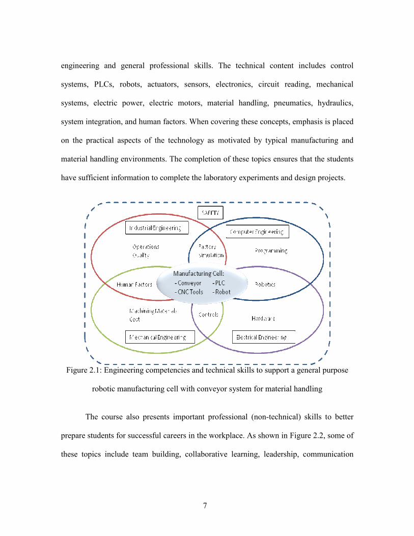
Figure 2.1: Engineering competencies and technical skills to support a general purpose
robotic manufacturing cell with conveyor system for material handling
The course also presents important professional (non-technical) skills to better
prepare students for successful careers in the workplace. As shown in Figure 2.2, some of
these topics include team building, collaborative learning, leadership, communication

8
skills, project management, procurement, and ethics. The first lecture cluster focuses on
team dynamics such as team building activities, project management, proper
communication techniques, and leadership. Next, students learn how to properly procure
materials and equipment, and review general ethics. Finally, the classroom introduction
of professional skills can be practiced and utilized in the team-based laboratory
experiments and projects.
To reinforce the learning concepts, periodic multi-week homework assignments
have been assigned for completion by student teams. Although not currently required, the
student teams might be changed for each assignment to facilitate team building skills.
Lastly, a midterm exam features an in-class test, laboratory practical, and take home open
ended problem. To assess the general performance of student learning throughout the
course, frequent surveys and pre/post course questionnaires may be administered.
Figure 2.2: Select topics introduced in mechatronics and material handling system course
Laboratory Experiments
The mechatronics laboratory allows students to explore sensors, actuators,
robotics, PLCs, conveyors, and system integration. A representative sampling of the
Technical, Business & Interpersonal Skills
Technical Skills Toolbox
General Ethics
Team Building Collaborative Learning Communication Skills
Leadership
Procurement Project Management

9
experimental modules will be presented with learning objectives, procedure, and
materials list.
Programmable Logic Controllers
PLCs are used in most industrial processes to control product manufacture and
movement. Two laboratory modules are available that feature PLC programming basics
and networked PLCs targeted for conveyor system control.
Physical Security System
The students create an alarm system (refer to Figure 2.3) through the wiring of
security components and designing ladder logic to accomplish prescribed security
functionality. This module allows students to gains hands-on experience with PLCs using
common safety hardware. An Allen Bradley Micrologix 1000 PLC has been selected.
The system features four inputs: motion detector, magnetic contact, vibration detector,
and panic button. All four devices are wired internally as a normally closed (NC) circuit.
Once a device is activated, the internal contacts open and power stop flowing back to the
PLC. These sensors are pre-mounted and wired to a second terminal block. Four on/off
toggle switches emulate an input keypad for the security system. The system outputs
include one light stack unit (green, yellow, and red lamps).
Learning Objectives
The student will understand how PLCs operate and typical signal configurations.
A selection of input and output devices will be introduced, wired, and integrated into

10
ladder logic instructional blocks. With these skills mastered, the second laboratory
module will create a network connecting multiple PLCs.
Laboratory Procedure
1. Design an alarm system to detect an introducer while offering the home or business
owner conveniences for arming and disarming it as needed.
2. Connect the inputs and outputs using terminal blocks and wires.
3. A ladder logic program will be created to function in the following manner:
a. System armed by placing all toggle switches to ‘open’ position with green
light illuminated.
b. Once an input has been triggered, the yellow light will turn on for a period of
5 seconds. Before this interval is completed, the toggle switches must be
changed to a ‘code’ that will deactivate the alarm (e.g., 1010).
c. If the proper code is entered within 5 seconds, the yellow light will turn off.
d. Once the switches are put back to 0000, the system will arm itself again.
e. If the proper ‘code’ is not entered in a timely manner, the red light on the light
stack will switch on and the alarm will sound.
f. Once the alarm has been tripped, the system cannot be reset by the switches.
4. RSLogix500 and RSLinx will be used to create the ladder logic and download the
program to the PLC. The security inputs will be monitored with “Examine If Open”
(XIO) instructions, while the ‘code’ will require both XIO and “Examine If Closed”
(XIC) instructions. The lamp outputs will use “Output Enable” (OTE), “Output

11
Latch” (OTL), and “Output Unlatch” (OTU) instructions. Also, timers will be
introduced and their respective status bits set for a five second period.
Materials
The laboratory materials include a motion detector (Optex #FX-40), panic button
(Omron #A22-MR-01M), MicroLogix 1000 (Allen-Bradley #1761-L32BWA Series E
FRN 1.0), magnetic contact (Honeywell #943WG-WH), vibration detector (Enforcer
#PAT-14658), switches (McMaster #7343K184), and light (Patlite #XEFB-D).
Figure 2.3: Security system with motion, vibration and entry sensor, light stack, horn,
panic button, four binary switches, and programmable logic controller
Networked PLCs for Distributed Architecture
In a typical manufacturing environment, multiple PLCs are networked together
for communication and the coordination of events. Although there are different network

12
protocols (e.g., DH-485, DeviceNet, EtherNet), an understanding of one network protocol
can be extrapolated to others. This laboratory module creates a network; PLC1 governs
the material handling system direction while PLC2 powers the rollers to operate a
modular conveyor system. Each PLC is a MicroLogix 1500 connected to individual ENI
modules via RS-232 cables. These modules convert messages sent by the PLC to the
EtherNet protocol, and then translate the messages sent by the network to the PLC. The
network (ENI modules, network switches, CAT5 network cable, PC) was connected to
allow the PC to access the PLCs as shown in Figure 2.4. Using the security system
experiment, the toggles switches and red/green lamps on the light stack were wired into
the inputs/outputs of PLC1. For the second PLC, a single conveyor segment is connected
which featured five powered rollers and seventeen gravity idle rollers. Along the edge,
mounted infra-red sensors determine the position of materials. The sensors and powered
rollers have been pre-wired into PLC2. A connectivity chart summarized how the rollers
and sensors are connected to the PLC input/output channels.
Learning Objectives
The student will gain an understanding of PLC networks with the ability to
configure a network. Specifically, they will establish communication between two PLCs
over a prototype network interfaced to a conveyor system with integrated sensors to
control material movement. Further, this experiment shall reinforce basic skills in the
programming and operation of PLCs.

13
Figure 2.4: Two programmable logic controllers (PLCs) with Ethernet modules and
central network switch connected to a computer work station for programming
Laboratory Procedure
1. The first PLC is connected to the toggle switches and light stack. Then, PLC1 and
PLC2 are connected to their respective ENI modules. Finally, the ENI modules and
PC are interfaced to the network switch to permit PLC programming via PC.
2. Algorithms are created for the PLCs to perform the five tasks listed below. Most
instructions are familiar. However, the Message (MSG) instruction sends data in an
integer (N7) address from one PLC to another. By changing the N7 register bits, data
can be communicated between two PLCs. For example, PLC1 can change two bits
(based on the toggle switches) and monitor two other bits that control lights.
Similarly, PLC2 will monitor two toggle switch bits and change two light bits.
Switch ENI Module
PLC #1 PC
PLC #2
ENI Module

14
a. When one switch (connected to PLC1) is activated, the conveyor system
(powered by PLC2) will turn on and move a tool pallet down the line
b. While the pallet is moving, the red light (connected to PLC1) will turn on.
c. Once the pallet reaches the last sensor on the line, the conveyor will stop.
d. When the second toggle switch is activated, the conveyor will switch
directions and move the pallet back to its original destination.
e. Once pallet reaches this point, the green light connected to PLC1 will turn on.
Materials
The laboratory materials include MicroLogix 1500 (Allen-Bradley #1764-
24BWA), ENI Module (Allen-Bradley #1761-NET-ENI), and Network Switch (Standard
5 Port 10/100 Mbps Fast Ethernet Switch).
Robot Programming and Sensor Integration Experiments
Many factories use fixed base and/or mobile industrial robots with computer
controlled actuators to accomplish a variety of manufacturing and material handling
applications. Some typical operations include part “pick and place” operations and
general component assembly. In the next two laboratory experiments, students gain
experience with programming and utilizing a standard industrial robot. The students
move the robotic arm to specific points and assemble a piston (piston, connecting rod,
wrist pin) for an internal combustion automotive engine.

15
Industrial Robot Programming
The Staubli RX-130 robot features six degrees-of-freedom. The control cabinet
contains a pendant for manual programming and a terminal for software programming.
The teaching pendent allows the student to define specific points needed to control the
robot’s movement. The controller allows the user to move the specific joints of the
robotic arm through the V++ programming language. Using a few basic commands such
as OPENI, CLOSEI, MOVES, and DELAY, and by defining points using the pendant,
the robot can be controlled to perform various operations. A pneumatic end effect gripper
(refer to Figure 2.5) has been installed to grip different objects. This module also
introduces students to robot safety issues.
Learning Objectives
The student will understand robot fundaments such as movement (pendant and
language programming), motion limitations, and safety concerns. It will be observed that
the robotic arm may select different paths between operating points which reinforces the
need to remain alert.
Laboratory Procedure
1. Students need to review the safety requirements for the robotic cell.
2. After ensuring that power is disconnected, students enter the cell to stage the
necessary parts to assemble and ship the pistons (i.e., pistons, rods, pins, pallet).
3. The appropriate end effect gripper should be installed on the robotic arm and the
compressed air supply turned on.
16
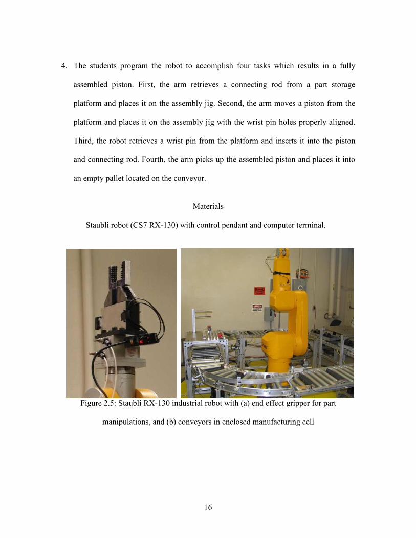
4. The students program the robot to accomplish four tasks which results in a fully
assembled piston. First, the arm retrieves a connecting rod from a part storage
platform and places it on the assembly jig. Second, the arm moves a piston from the
platform and places it on the assembly jig with the wrist pin holes properly aligned.
Third, the robot retrieves a wrist pin from the platform and inserts it into the piston
and connecting rod. Fourth, the arm picks up the assembled piston and places it into
an empty pallet located on the conveyor.
Materials
Staubli robot (CS7 RX-130) with control pendant and computer terminal.
Figure 2.5: Staubli RX-130 industrial robot with (a) end effect gripper for part
manipulations, and (b) conveyors in enclosed manufacturing cell

17
Robot and Conveyor System Integration
This module builds on the knowledge gained regarding the Staubli robot and
previous PLC modules to integrate the equipment into a material handling system. A
series of conveyor segments, featuring distributed electrical powered rollers with driver
modules, are constructed of inner/outer aluminum rails mounted on an aluminum frame
with casters. The infra-red sensors, mounted on the edge of the conveyor, permit the
position tracking of materials on the conveyor rollers. The Staubli control cabinet
features input/output terminal blocks to allow the robotic arm to be integrated into
surrounding environment for closed loop operation. The dual PLCs, controlling the
conveyor segments, will be interfaced to the robot, for coordinated material movement
studies.
Learning Objectives
The student will understand the integration of robotics with material handling
systems for product fabrication and transport. A unified architecture will be introduced
and implemented which permits multiple PLC interactions with robot arm to assemble
and move goods based on user defined algorithms and sensor feedback.
Laboratory Procedure
1. Two robot outputs (e.g., 1 and 2) are connected to PLC1 thereby replacing the two
toggle switches used for the network conveyor. Similarly, two robot inputs (e.g., 1010
and 1011) are wired to PLC1 to replace the lights.

18
2. The robot is now programmed to wait before placing the piston in the pallet until a
signal is sent from PLC1 which indicates the pallet is in the proper position based on
the infra-red sensors.
3. Once the assembled automotive piston is properly secured in the pallet, another signal
is sent to PLC1 by the robot to move the pallet to the end of the conveyor system for
subsequent operation by another manufacturing resource.
4. When the pallet reaches this terminal conveyor position, the robot is programmed to
return to the “ready” position to resume operation.
Materials
The materials for this laboratory include Holjeron 24VDC brushless dc motor
driven rollers, Holjeron #ZL-DK100 driver modules, 8020 T-Slot extruded aluminum,
and Takex #GS20SN infra-red sensors.
Electronic Circuits
Electronic circuits are common in manufacturing environments and consumer
products which should encourage engineers to understand their basic electronics.
Consequently, electronic components and integrated circuits will be introduced and
reviewed to acquaint students with their general operation. In the next two modules,
several basic circuits will be presented which offer breadboarding opportunities with
signal test points. The two circuits feature ‘electronic dice’ which mimics a real dice
using IC chips and a rotational sensor to count rotations of a flywheel.

19
Electronic Dice Circuit
The electronic dice module introduces integrated circuits with the creation of an
electrical system that emulates the functionality of a six sided dice with a digital display.
The circuit features a general purpose timer chip, a counter chip, assorted resistors,
diodes, a switch, and six LEDs as shown in Figure 2.6. The timer chip is configured to
output a high frequency oscillating signal, which is then fed to the counter chip. The
counter will count up, until the switch is activated. At this point, the counter’s outputs are
latched. These outputs are connected to LEDs, in such a way as to resemble a die. Due to
the high frequency of the oscillating signal each time the switch is activated, a new
number will appear on the die, thus creating a random pattern.
Learning Objectives
The student works with a 555 timer chip and learns how to test basic circuit
features. Specifically, they learn how to use breadboards, wire chip inputs/ outputs, and
validate circuit functionality using oscilloscopes and multi-meters.
20
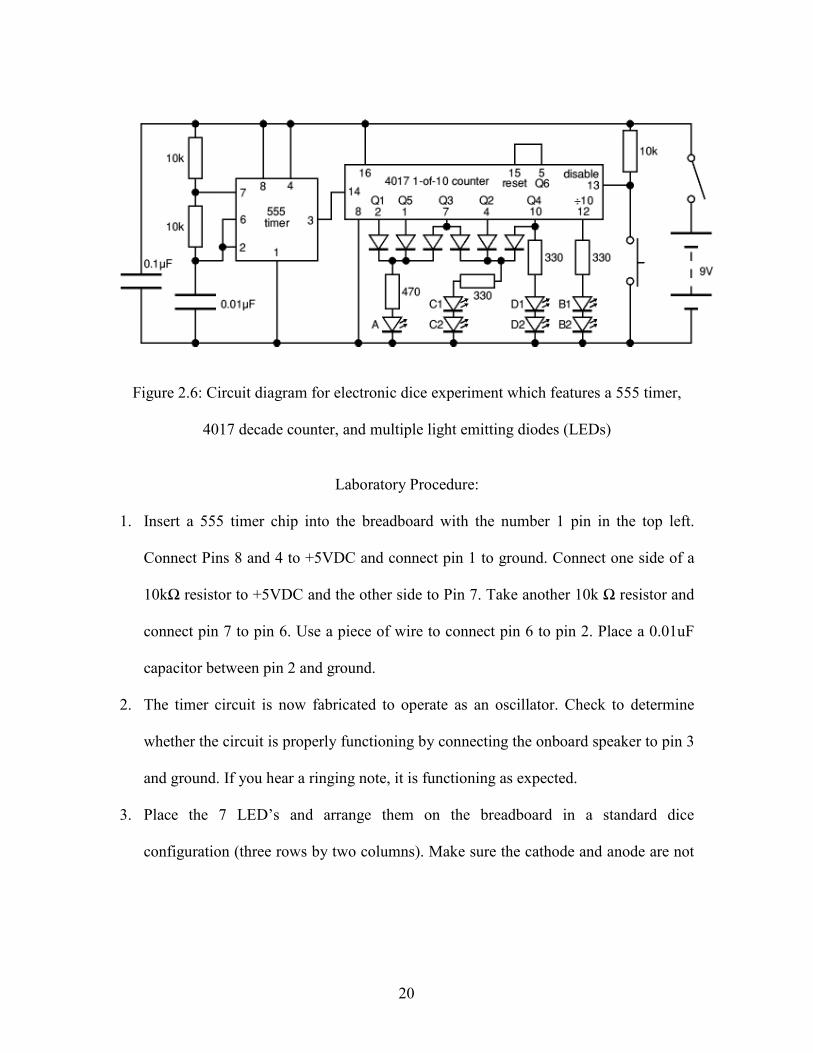
Figure 2.6: Circuit diagram for electronic dice experiment which features a 555 timer,
4017 decade counter, and multiple light emitting diodes (LEDs)
Laboratory Procedure:
1. Insert a 555 timer chip into the breadboard with the number 1 pin in the top left.
Connect Pins 8 and 4 to +5VDC and connect pin 1 to ground. Connect one side of a
10kΩ resistor to +5VDC and the other side to Pin 7. Take another 10k Ω resistor and
connect pin 7 to pin 6. Use a piece of wire to connect pin 6 to pin 2. Place a 0.01uF
capacitor between pin 2 and ground.
2. The timer circuit is now fabricated to operate as an oscillator. Check to determine
whether the circuit is properly functioning by connecting the onboard speaker to pin 3
and ground. If you hear a ringing note, it is functioning as expected.
3. Place the 7 LED’s and arrange them on the breadboard in a standard dice
configuration (three rows by two columns). Make sure the cathode and anode are not

21
on the same rail and that no LED shares the rail with another. There should be three
sets of LED’s in series with the middle LED being alone.
4. Wire a 330Ω resistor to points A, B, and D. Next, connect a 470Ω resistor to point C.
Apply +5VDC through the resistors to the LED’s and verify that all seven are
illuminated. If so, then this circuit section is properly completed.
5. Place the 4017 counter with pin 1 oriented in the top left corner. Connect pin 16 to
+5VDC and pin 8 to ground. Wire the 1N4148 signal diodes to pins 1, 2, and 7. Bring
the diodes together on one rail and connect this rail to point C using the 470Ω
resistor. Connect the 1N4148 signal diodes to pins 4, 7, and 10. Bring the diodes
together on one rail and connect this rail to point D using the 330 Ω resistor. Wire pin
10 to point B using a 330 Ω resistor. Connect pin 12 to point A using a 330Ω resistor.
6. Use a 10kΩ resistor to connect +5VDC to pin 13. Wire the switch from pin 13 to
ground. Connect pin 14 of the 4017 chip to pin 3 of the 555 timer. Connect a 0.1 uF
capacitor to between ground and +5VDC to smooth the power supply.
7. When the circuit is energized, all 7 LED’s should be illuminated until the switch is
pressed again. At that point, there should be a different number displayed via the LED
configuration which resembles the behavior of a thrown dice.
Laboratory Materials
The electronic supplies for the experiment include 330Ω resistors (3), 10kΩ
resistors (3), 470Ω resistor, 0.01µF capacitor, 0.1µF capacitor, 555 Timer (Texas
Instruments #TLC555CP), 4017 decade counter (Texas Instruments #CD4017BE), toggle

22
switch (C&K Components #GT12MABE), signal diodes (6) (Diodes Inc, #1N4001-T),
and LEDs (7) (Panasonic #LN81RCPHL).
Rotation Sensor Electronic Circuit
An electronic sensor circuit will be created to count the rotations of a metal
flywheel connected to a servo-motor. A metal test stand holds the dc motor, metal disk
with single through hole, and light emitting diode (LED) with photo-resistor sensor as
shown in Figure 2.7. An accompanying breadboard circuit (refer to Figure 2.8) interfaces
to the LED and sensor to count the flywheel rotations with test points to validate during
construction.
Learning Objectives
The student will gain experience with op-amps (compare measured sensor voltage
against established threshold value) and a combined counter and display driver integrated
circuit (4026 chip) for multiple segment LED display. In addition, a sequential building
process that emphasizes frequent validation will reinforce the need to test each subsystem
for operation prior to the complete build.

23
Figure 2.7: Servo-motor driven wheel featuring a single thru-hole with LED lamp and
photo-resistor components for rational sensor experiment
Laboratory Procedure
1. Insert the 741 operational amplifier into the breadboard with the number 1 pin in the
top left. Connect Pin 7 to +9VDC and connect pin 4 to ground. Take the leads coming
from the LDR and connect one to +9VDC and connect the other to pin 3 of the 741
amplifier.
2. Use a 3kΩ resistor to connect one side to +9VDC and the other side to pin 3 of the
741 chip. Connect a 330Ω resistor to +9VDC and connect the other end to the
positive lead for the white LED. Attach the other LED wire to ground.
3. Test the circuit. Place a LED with 330Ω resistor to pin 6 of the 741 amplifier. Spin
the wheel and check to ensure the LED is flashing when appropriate. If the LED fails
to light, increase the resistor to pin 2. If the LED is always on, decrease the resistor to
pin 2. Once the circuit is verified, remove the LED and resistor.

24
4. Place the 4026 IC into the breadboard with the number 1 pin in the top left. Next,
connect pins 3 and 16 to +9VDC. Now connect pins 2, 8, and 15 to ground. Finally,
place the seven segment display onto the breadboard and follow the diagram to
connect the pins. Please include 330Ω resistors in each connection.
5. The 4026 IC pin 1 should be connected to +9VDC; ensure that it counts up one. If the
circuit successfully counts up one, then connect pin 1 of the 4026 IC to pin 6 of the
741 op-amp chip.
6. The circuit has been successfully constructed. Connect the servo-motor to a variable
output dc power supply to spin the attached flywheel. As the wheel rotates, watch the
circuit count the total number of rotations.
Laboratory Materials
The supplies include 330Ω resistors (8), 3kΩ resistor, 741 op-amp (Fairchild
Semiconductor #LM741CN), 4026 IC chip (Texas Instruments #CD4026BE), 7 segment
display (Lite-On Inc #LSHD-5503), light dependent resistor (Chartland #N5AC501085),
LED (Panasonic #LN81RCPHL), and dc motor test stand.

25
To counter circuit
3K
1K-10K
LDR
9 V
741 Op Amp
1234
5678
LED 5K
5K
330
Figure 2.8: Rotational photoelectric sensor circuits - (a) sensor and (b) counter elements
Design Project - Material Handling System with Order Fulfillment
A semester long experimental based design project has been introduced to
supplement the classroom activities and laboratory modules. In the laboratory, the robot
and conveyor system have been combined on a somewhat ‘microscopic’ level to execute
a specific well-defined task. In contrast, the design project requires student teams to
create a larger ‘macroscopic’ system that encompasses tasks including order
identification, fulfillment, and movement in preparation for shipment from the
manufacturing facility. The project emphasizes the need for students to divide into teams

26
to accomplish singular objectives that may then be integrated into a collective material
handling system which achieves a larger objective. For instance, some of the groups may
focus on sensing and sorting, conveyor systems, PLC programming, or robot interaction
The team approach allows students to experience how real world problems may be solved
with typical group and organization challenges. Finally, the project allows the application
of class room and laboratory technical and interpersonal skills to create a mechatronics
system.
Figure 2.9: Staubli robot with end effector and color balls with sorted single color bin
The design project requires the sorting and packing of colored (blue, green, red,
and yellow) multi-sized plastic balls for order fulfillment at a toy distribution center.
Specifically, the students use the Staubli robot, conveyor segments, and sensors/actuators
to create a small scale material handling system per Figure 2.9. In terms of operation, a
bar code on the pallet box side lists the number of colored balls and destination (one of
three points) on the conveyor system for subsequent pallet placement. The system reads

27
the bar code using a bar code scanner (Keyence #BL-160). A color sensor (Keyence
#CZ-H32) determines the ball color loaded in the main hopper and places the correct
number in the proper container (refer to Figure 2.10). The box is then sent down the
conveyor system and routed to one of three spurs as commanded by the PLC network.
Refer to Chapter Four for a more detailed examination of this design project.
Figure 2.10: Shipping container with ball order fulfilled and complete sorting system
Summary
The growing sophistication and complexity of engineering systems requires broad
knowledge of mechatronics (sensors, actuators, and controls with application to consumer
products, specialized equipment, and manufacturing environments) as well as general
business and interpersonal skills. In this paper, the mechatronics (and material handling
systems) course has been described which offers students an experience composed of
classroom activities, laboratory experiments, and semester long design project. First, the

28
technical, business, and personal skills covered include electrical, industrial, mechanical,
and systems engineering, project management, procurement, team building, and
leadership. Second, laboratory experiments allowed students to program networked
PLCs, integrate conveyor system components including industrial robot for material
movement, and breadboard electronic circuits. Third, a challenging material handling
design project offered a learning opportunity for students to synthesize class and
laboratory materials in a hands-on team-based endeavor. A comprehensive mechatronic
course should help prepare graduates to meet the product design, manufacturing, material
transport, and research needs of the 21st century.

29
CHAPTER THREE
DATA ACQUISITION EXPERIMENTS
Data acquisition techniques can be utilized in industry to ensure product quality or
to record measurements of a system process. Two exercises were created to cover these
important topics in mechatronics, however were not included in the previous chapters. In
the first experiment, students measure the vibration frequency of various length chime
rods, while in the second the frequency of a torsional pendulum and a hanging pendulum
are measured.
Acoustics Laboratory
In the first laboratory students were tasked to measure the vibrating frequencies of
several chime rods, each with varying lengths. This lab contained two different sections;
the first part involves using a microphone to determine the frequency of resonance of
each rod, while the second section utilizes an accelerometer to determine the frequency.
Several different technologies are introduced, such as a pre-amplifier (refer to Figure 3.1)
and an accelerometer, as well as specific testing locations, such as an acoustic chamber
(refer to Figure 3.2).
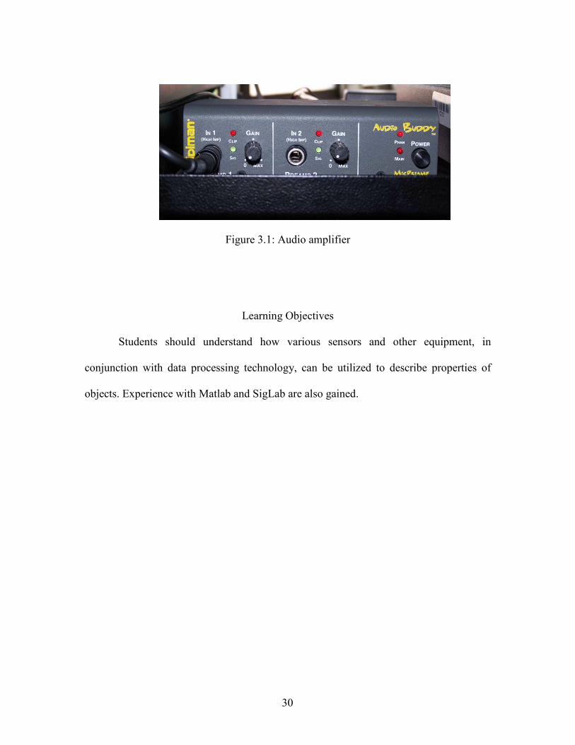
30
Figure 3.1: Audio amplifier
Learning Objectives
Students should understand how various sensors and other equipment, in
conjunction with data processing technology, can be utilized to describe properties of
objects. Experience with Matlab and SigLab are also gained.

31
Figure 3.2 Set up for acoustic experiment
Procedure – Acoustics Experiment
1. Hang chime rod on the rear hook inside semi-anechoic chamber.
2. Place the microphone on the stand.
3. Connect the microphone to input 1 on Audio Buddy pre-amp box.
4. Connect the red cord from output 1 on Audio Buddy to the computer (microphone
input).
5. Set microphone inside semi-anechoic chamber as close to the chime rod as possible
without touching it.
6. Open Sound Recorder from Windows start menu.
7. Press Record and strike the chime rod.
8. Press Stop after collecting sound data.

32
9. Save Sound Recorder file as chime.wav in the MATLAB folder.
10. Open wavanal.m file in MATLAB.
11. Run the program and observe the resulting graphs of the spectrum analysis and
frequency of the chime rod.
12. Repeat experiment using a different chime rod. Observe any differences in the
spectrum analysis and frequency graphs.
Procedure — Vibration Experiment
1. Install accelerometer (100mV/g) on chime rod. Hang chime rod on the rear hook
inside semi-anechoic chamber as shown in Figure 3.3.
Figure 3.3 Rod with accelerometer in the chamber
2. Connect the accelerometer cable to channel 2 on SigLab per Figure 3.4.

33
3. Connect the impact hammer cable to channel 1 on SigLab.
Figure 3.4 Connections at Siglab
4. Type “sigdemo” on the command window of MatLab.
5. Press VNA (Virtual Network Analyzer) button in Siglab.
6. Open MechatronicsLab.vna file in SigLab (parameters for this experiment are saved
in this file).
7. Hit “AVG” and strike chime rod using impact hammer. Observe for changes in the
graphs.
8. Hit “STOP”.
9. Copy the plots (impulse response from the hammer and FFT response from the
accelerometer) or export data to be analyzed later.
10. Detach the accelerometer from the chime rod and install it on the next rod to be
tested. Repeat procedures 7-9 until all the 5 rods have been tested.
Materials

34
A standard Chime Rod set with five varying lengths of chime rods were used. The
first section utilized a microphone connected to an amplifier, which was then connected
to a PC equipped with MatLab. For the second section, an accelerometer was attached to
the chime rod, and connected to a SigLab box. An impact hammer was also attached to
this box. A software program connected to this SigLab device allowed for data
acquisition.
Pendulums Laboratory
The pendulum is a classic device to study motion and the concept of energy. In
this experiment, two different types of pendulums are used to understand data acquisition
as shown in Figure 3.5. In the first, a Hall Effect sensor is used. This type of sensor is
able to detect small changes in magnetic fields. For the second pendulum, an
accelerometer is utilized.
Learning Objective
Students will understand how various sensors can be connected to a data
acquisition card, which can then be utilized by LabView. Students will also gain
experience in working with a Hall Effect sensor, as well as an accelerometer. Finally,
higher level concepts such as noise and data collection errors should be understood.

35
Figure 3.5 Pendulum experiment setups
Procedure – Torsional Pendulum
1. Connect the torsional pendulum to the test stand. Assure that the pendulum is secured and the Hall effect sensor is in an adequate position to measure data.
2. Ensure that the Hall Effect circuit is set up and connected correctly to both the power supply and the sensor.
3. Turn the power supply on and set it to 3 volts.
4. Wind the pendulum 3-5 full rotations in either direction. Release the pendulum and, using the DAQ, record at least one full oscillation.
5. Calculate the angle per tooth on the gear to which will be used to determine the
angular displacement.

36
6. Transfer data to Excel. Differentiate the data from the accelerometer to go from acceleration to velocity to displacement. Then integrate the data from the magnetic
variable reluctance sensor to go from displacement to velocity to acceleration. Compare the two results.
Procedure – Swinging Pendulum
1. Connect the swinging pendulum to the test stand and mount the rotational
potentiometer to the swinging joint.
2. Turn on the constant current PCB amplifier.
3. Rotate the pendulum to about 45º and release. Using the DAQ, record a minimum of
five full oscillations.
4. Transfer data to Excel. Integrate the data from the accelerometer to obtain velocity and displacement. Compare the two results with those of the torsional pendulum.
Materials
Two types of pendulums were used; a torsional (comprised of a metal gear on a
thin wire) and swinging Pendulum (weight attached to a rod). A Hall Effect sensor or an
accelerometer was attached to collect data. In either case, the sensor was connected to a
pre-amplifier, which was then connected to a computer with LabView software. The
software was programmed to output data collected from the sensor to an excel file which
could be manipulated to determine desired data.
These two laboratory experiments help to solidify the understanding of data
acquisition. Several types of sensors are used, as well as two different computational
programs; Matlab and LabView. Students learning various data acquisition environments
and different programs ensure they will be more adequately prepared upon graduation.

37
CHAPTER FOUR
A MECHATRONICS AND MATERIAL HANDLING SYSTEMS LABORATORY
Introduction
Modern industrial systems rely on core technologies such as programmable logic
controllers (PLCs), computer networks, industrial robots, conveyor systems, and a variety
of sensors and actuators to assemble and move products within flexible work cells. In
many instances, these devices must be integrated to realize a computer controlled
mechatronics solution. To create and maintain these systems, engineering teams must
apply their individual and collective skill sets. Material handling systems offer a great
subset of processes to demonstrate how mechatronic solutions are designed and
implemented to move, track, and manipulate products. Mechatronic technologies can be
used to read a barcode, divert products off a conveyor line, place items in a container, and
perform other material handling tasks. While these devices are common in industry,
universities do not typically offer formal courses of instruction which explore their
operation and integration.
A brief literature review will be presented on academic mechatronic programs.
Acar and Parkin [14] provided an overview of mechatronics and select programs from
universities around the world. Pennsylvania State University has created three courses
that provide students with fundamental concepts in materials processing, production
design, and manufacturing [6]. Merckel and Fisher [3] at the Rose-Hulman Institute of
Technology created a two week PLC experience, which utilized two separate PLC
38
stations for student ‘hands-on’ experience. Erickson [7] described a University of
Missouri-Rolla laboratory which used four industrial processes featuring robotic arms,
assembly and inspection, pH neutralization, and operator interfaces. Carnegie Mellon
University utilized a robotics laboratory that supplied the students with ‘hands-on’
experience [15]. Chiou et al. [4] at Drexel University have developed a mechatronics
course that controls industrial robots over the internet using machine vision systems, PLC
modules, webcams, and sensors. Some international mechatronic programs have been
highlighted by Khan [2] with a review of micro-controller technology,
mechanical/manufacturing engineering, transducers, and PLCs. Lee and Park [5] created
a computer controlled robotic laboratory which focused on systems integration concepts.
The Utah State University used mobile robots for mechatronics education as described by
Stormont and Chen [8]. Ghone et al. [16] discussed ‘hands-on’ experiences in a multi-
disciplinary mechatronics laboratory at Clemson University which contains circuits,
pneumatics, hydraulics, and servo-motors [9]. A series of experiments utilizing PLCs,
industrial robotics, and electrical circuits which culminated in a mechatronics design
project was discussed by Shirley et al. [17]. Murray and Garbini [18] reported on the
mechatronic capstone design projects at the University of Washington, which featured
four classes to teach fundamentals. Ebert-Uphoff et al. [19] compared various aspects of
mechatronics courses from both a teaching and infrastructure viewpoint. For a graduate
level focus, Du [20] offered a thorough review of various laboratory experiments and
possible projects.

39
Creating a firm foundation is critical to future mechatronic applications. In model-
integrated mechanics [21], both model-driven architectures and pre-defined function
blocks are used to design systems. Finally, Jammes and Smit [22] proposed that service
oriented automation, in which mechatronic components exemplify a plug-n-play
architecture, should be required to accommodate ever changing manufacturing processes.
To ensure students understand basic mechatronic fundamentals, the multi-disciplinary
“Mechatronics and Material Handling Systems” course was created at Clemson
University to introduce mechatronics systems from an industrial setting and encouraged
students to practice team skills. The classroom time focuses on core technologies and
improving communication skills. An accompanying laboratory features eight experiments
involving PLCs, industrial robotics, data acquisition, and electronic breadboard
experiments. A case study encourages students to synthesize class and laboratory
concepts into a focused material handling task (refer to Figure 4.1). Teamwork is stressed
and practiced in the laboratory experiments and case study.

40
Figure 4.1: Engineering technology topics in the mechatronic and material handling
course to support case studies
The remainder of the manuscript is organized as follows. A selection of four
laboratory experiments and accompanying technologies will be discussed followed by a
presentation of two case studies which focus on assembly and sorting operations. A
summary is presented to conclude the paper. The Appendix contains the material lists for
the experiments.
Experiments – PLCs and Robotics
Eight laboratory experiments were created which feature four distinct
technologies used in industrial mechatronic systems. The experiments cover four
different topics: PLCs and communication; industrial robotics; data acquisition; and

41
electronic circuits. These laboratories establish the frame work for system integration
activities in the case studies. Four of the eight laboratory modules will be discussed and
the accompanying materials listed in the Appendix. The reader is referred to Wagner [23]
for information regarding the other experiments.
PLC Programming and Communication
An understanding of PLC operation is essential to the design of a manufacturing
mechatronic system. The combination of multiple PLCs across a dedicated network can
significantly increase the response time and effectiveness of a control system. Two
laboratory modules were created that focus on PLC basics and creating a dedicated
network. In the first module, fundamental PLC control is taught through the creation of a
residential security system, while in the second, a PLC network is implemented to control
a conveyor system.
Residential Security System
A modular security system is constructed to help students understand PLC
operation. The successful completion of this laboratory should allow students to
understand PLC programming and connecting various inputs/outputs to create a
mechatronic system. The operational principal behind a security system is common to
most students; thus, making it an ideal choice to explain PLC operation and how PLC
inputs can control various outputs. A motion detector, a vibration detector, a magnetic
switch, a pushbutton, and four switches represent the system inputs, while alarm lights

42
function as the output. A PLC (Allen-Bradley MicroLogix 1000) acts as the controller for
the system.
The students wire the inputs and outputs to the PLC and create a program that
controls the system operation (refer to Figure 4.2). The security system is to operate in
the following manner: when a sensor is triggered, the user has five seconds to input the
proper code before an alarm light activates and “locks out” the system. Students are
exposed to many programming commands used for ladder logic devices (e.g., Examine-
If-Open, Examine-If-Closed, various timer implementations). Proper wiring techniques
and PLC operation is also explained. Students are encouraged to discuss in their small
groups the most efficient manner to wire and program the PLC.

43
(a)
(b)
Figure 4.2: Security system experiment - (a) schematic, and (b) photograph with
component layout and space for wiring

44
PLC Network for Conveyor Control
The second module re-enforces basic PLC programming principles and introduces
students to PLC networks. A PLC network allows efficient communication between two
(or more) PLCs which ensures data sharing. In this experiment, the teams move a “tool”
pallet down a conveyor line, wait for an input signifying some action has taken place, and
then activate the conveyor to move the pallet back to the original starting location.
The conveyor line was constructed with both motorized and idler rollers, as well
as infrared sensors located at various positions along the rails. Following the completion
of this laboratory, students should be able to electrically interface two PLCs together over
an Ethernet network, and send/receive data packets to accomplish a given task. Two
PLCs (Allen-Bradley MicroLogix 1500) control the system (refer to Figure 4.3). The
switch inputs (turn off/on the conveyor) are connected to PLC-1 as well as two output
lights to indicate when a task is complete. PLC-2 controls the motorized conveyor rollers
and monitors the infrared sensors attached to the conveyor system. The PLCs are
networked over a dedicated Ethernet system using two ENI modules from Allen-Bradley.
The network functions in the following manner. An Integer register from one PLC
is sent, through the ENI modules, to the other PLC. Information (by using bits) or
numbers (by using the entire register) can be transmitted between PLCs by sending these
designated Integer registers. All control information (i.e., which Integer register to send
to which PLC, which register at the target PLC the information goes to) was stored in a
ladder logic function block. The ‘control’ inputs wired to one PLC, and the motorized

45
rollers connected to the second PLC, forces students to comprehend and utilize the
network.
Although a variety of PLC networks exists (e.g., ControlNet, DeviceNet,
Fieldbus), the current equipment offers sufficient hands on practice for students to grasp
the concept. The knowledge gained may then be transferred to more complicated
networks with additional PLCs and/or different protocols. Finally, the teams were
encouraged to discuss various solutions to problems encountered among the group
members.
Figure 4.3: PLC network featuring two controllers (regulate lights and rollers) with
CAT5 cable network
Robotic Manipulator
Factories utilize fixed and mobile industrial robots to perform specific tasks such
as pick-and-place operations, welding, and product manipulation. Two laboratory

46
modules were developed which illustrate the intricacies of integrating an industrial robot
into a mechatronic system. In the first module, students program the robot to assemble an
automotive piston. The second module integrates this industrial robot with a modular
conveyor system for product movement.
Industrial Robot Primer
The Staubli robot/safety review and operation is completed in the third laboratory
module. The Staubli RX-130 industrial robot features six degrees of freedom that allows
for various pick-and-place operations. Once completed, students should be able to use
this industrial robot to complete a complicated task.
The RX-130’s movements are created and programmed using the V++ computer
language and manual input (pendant) connected to the robot’s control cabinet. Students
are given instruction in programming basics, including the teaching pendant, defining
special locations, and creating code. Once familiar with the robot, the group is tasked to
assemble an automotive piston. A previously constructed jig assisted in the assembly
process. Students program the various spatial points to maximize efficiency and ensure
safety. Most participants were impressed that a complicated task such as assembling an
automotive piston could be accomplished by programming a few simple points.
System Integration with Robotic Manipulator
The fourth laboratory module focuses on connecting external inputs and outputs
to the Staubli robot control cabinet. Unmodified, the robot operates in an open loop
manner with the exception of position information received from each arm joint.

47
However, the robot is capable of receiving feedback through input/output (I/O) boards
allowing environment information to be received. Input from various pushbuttons,
sensors, switches, and PLCs can be used in conjunction with internal software programs
to increase the robot’s effectiveness. Following the completion of this laboratory module,
students were able to connect the industrial robot to an external mechatronic system,
thereby drastically increasing the system utility and complexity.
The laboratory exercise integrates the PLC network controlled conveyor system
with the Staubli robot through the use of two signal wires. One wire transmits a signal
from PLC-2 to the robot, while a second wire connects an output from the robot to PLC-
2. A four sequence process is implemented: the system moves a tool pallet down the
conveyor; a signal is sent to the robot to start piston assembly; the piston is assembled
and placed on a tool pallet; and the robot sends a signal to PLC-2 to move the pallet back
down the conveyor (refer to Figure 4.4). A light connected to PLC-2 activates when the
process is completed.
The conveyor is composed of modules created in-house by students, which offer
several advantages over procuring pre-constructed commercial conveyors. The design
and construction of the segments creates a practical experience for students and provides
cost effective solutions. The segments feature caster wheels, attached to the bottom, to
aide in reconfiguring the conveyor. This helps to ensure that the case studies can be
changed easily. Sensors are attached along the conveyor segments, notably at the ends, to
track product movements.

48
(a) (b)
Figure 4.4: Automotive piston assembly utilizing system integration - (a) automotive
piston construction jig, and (b) schematic.
Case Studies
An in-depth semester long project, viewed as a critical course element, allows
students to configure and control mechatronic components to create a material handling
system. Each study maintains a focus on material handling while incorporating different
technologies (color sensing, barcode, RFID) into the laboratory. In this section, two case
studies (construction of automotive piston assemblies; color ball order fulfillment system)
will be presented and discussed.
Product Creation – Assembly Operation
The first study challenges students to create a material handling system to
assemble internal combustion engine pistons. To complete this task, teams are required to
design, procure, assemble, control, and verify system components. For instance, students

49
fabricate parts, integrate sensors, program the robot, and design the PLC control system.
Interpersonal communication skills are practiced throughout the project to ensure the
proper timing of events.
In the laboratory space, teams configure the conveyor in an approximately
circular shape (refer to Figure 4.5) with three rounded corners and the fourth utilizing a
square pneumatic powered 90º turntable. The turntable uses two pneumatic cylinders
controlled by solenoid valves and a common manifold; one lifts the rollers up, while the
other turns the table 90º. By using the pneumatic cylinders to rotate the table, products
can be moved in any direction desired with bi-directional motorized rollers. Two sensors,
attached on each end, completed the turn table.
Motorized rollers, powered by individual 24 VDC driver modules, and idler
rollers control the movement of objects on the conveyor system. Two control wires from
the PLC determined when the given roller is activated and the direction it turns. The
powered rollers are wrapped with a friction tape to facilitate object movement. Infrared
sensors are attached at various positions along the conveyor.
The operation of the conveyor system is controlled by two Allen-Bradley
MicroLogix 1500 PLCs connected over an Ethernet network. Each PLC controls one half
of the system. Specifically, PLC-1 controls the segments containing points D and E, and
PLC-2 controls the segments containing points A and C. The conveyor modules’ inputs
and outputs are distributed between the two PLCs. For example, the light stack is
connected to PLC-1 while PLC-2 is interfaced to the robot control cabinet. This allows

50
for ‘closed-loop’ operation of the material handling cell. A computer located nearby
allows students to program the PLCs and to observe their ‘on-line’ operation.
The system functions in the following manner (refer to Figure 4.5b). First, the
robot picks up a pallet from a storage tray and places it on the conveyor at Point A. Next,
an infrared sensor connected to PLC-2 indicates that the pallet is securely placed down
and activates the conveyor rollers. When the pallet reaches the ‘Queue Point’ (Point C),
the program checks to determine if another pallet, or object, is at the ‘Assembly
Location’ (Point D). If there is an object present, then the pallet temporarily stops. Once
the ‘Assembly Location’ is clear, the system continues to send the pallet down the
conveyor. In this manner, a queue is formed resulting in a pallet always being ready for
loading with the next piston assembly. Point C (Queue Point) is controlled by PLC-2,
while Point D (Assembly Location) is connected to PLC-1, such that communication
over the network is necessary to ensure proper queuing. A guard rail is mounted for pallet
positional accuracy and orientation as it approaches the ‘Assembly Location’. Once the
pallet reaches the ‘Assembly Location’, a sensor connected to PLC-1 is activated, which
triggers a signal to the robot via the PLC network. If for any reason the pallet does not
reach the ‘Assembly Location’, then the robot does not attempt to load the piston.

51
(a)
(b) Figure 4.5: Product creation system - (a) schematic, and (b) robot loading pistons into
pallet with start point [A], parts tray [B], queue point [C], assembly point [D], and
destination point [E].
A
D
C
B
E

52
The piston parts are available on a “Parts Tray” (Point B), located above one of
the conveyor segments due to the robot’s limited reach. A piston assembly jig was
created and attached to the conveyor near the ‘Assembly Location’. This jig assists the
robot in assembling the pistons. A photoelectric sensor detects the proper placement of
the wrist pin. If the wrist pin is not inserted correctly, then the piston could break apart
during system operation leading to product damage and a potentially unsafe environment.
If the pin is not fully inserted, the sensor does not activate and the robot is programmed to
halt and wait for user input. Once completed, the pistons are placed by the robot onto
pallets (two pistons per pallet) and a signal is sent to PLC-2, which communicates over
the network to PLC-1 to start the conveyor system to move the pallet. The pallet
continues to the turntable, and around the corner to the ‘Destination Point’ (Point E).
The complexity of this assignment mandates that the teams work efficiently.
Proper communication is critical within and between design teams. Students are able to
take pride in their own individual contributions to the overall effort.
Product Fulfillment – Sorting Operation
A modular order fulfillment system, in which containers are filled with plastic
colored balls, is examined for the second case study. Each container is filled with varying
numbers of red, yellow, blue, and/or green balls based on information stored in barcodes
affixed to the containers. The conveyor system is configured into a trident shape (refer to
Figure 4.6), so that three different destinations can be achieved to emulate a shipping
department. The project is divided into two sub-tasks: one team focuses on determining

53
the color of the ball and properly sorting it; the second group controls the conveyor
system and utilizes the barcode reader to determine the colored balls that complete a
particular order. Again, internal and external team communication skills are essential to
ensure that the project is completed satisfactorily.
A pushbutton triggers the system to activate motorized rollers on conveyor
segment ‘S3’ to move an order container down the conveyor line (refer to Figure 4.6a).
Once the container passes an infrared sensor, PLC-2 activates a Keyence barcode reader
(Keyence #BL-180). The reader is connected to a processing unit (Keyence #DV-90),
which stores four barcodes in its internal memory. When the reader scans a barcode, the
processing unit activates an output that corresponds to that particular barcode. By
monitoring these outputs, PLC-2 knows which barcode is scanned and uses this data to
fill a container with the proper number of each color ball. After the barcode is read, the
conveyor system halts the container at a point within the robot’s reach.
The system is initialized with the multiple sized colored balls randomly located
into the main hopper. To increase system efficiency, it was determined that the balls
should be pre-sorted into four smaller auxiliary side hoppers; each hopper contains a
designated color.
A Keyence color sensor (Keyence # CZ-32) and control module (Keyence # CZ-
K1) are connected to the system. The control module conditions the sensor signal,
determines the color from a preset list in memory, and activates a particular output. The
preset list is manually set so that any one of the four ball colors can be sensed. The color
sensor utilizes an LED to observe the reflected light waves; the sensor is mounted behind

54
Lexan for protection. Once the ball’s color in the output feed of the hopper is determined,
it is placed in one of four smaller hoppers by the robot. If the ball color cannot be sensed,
either due to the ball not being in the proper location to be sensed or the sensor not being
able to get a clean read, the ball is picked up and returned back into the main hopper. The
misreading frequency is small enough that this is an acceptable error handling method.
The individual color ball hoppers are programmed to accommodate a maximum number
of balls. The robot counts the number of balls in each hopper, stores this number in its
internal memory, and once all the hoppers are full of balls, the robot transmitted a ‘Balls
are Sorted’ signal to PLC-2.

55
(a)
(b) Figure 4.6: Order fulfillment system - (a) interconnection of three straight, three curved,
and 90º turntable conveyor sections with robot, and (b) photograph with barcode reader
[F] and color sensor [G].
F G

56
When PLC-2 receives the ‘Balls are Sorted’ signal, a binary code is sent back to
the robot to specify the ball color to retrieve. The binary code architecture uses three
wires to specify four colors (two wires for the binary code; one wire for the ‘Data Ready’
signal). The code is received by the robot, and promptly ‘Acknowledged’ (with dedicated
data signal). The robot then retrieves a ball from one of the individual color hoppers and
places it in the container. Once the acknowledge signal is sent, the PLC transmits a
request for the next color ball. This process continues until the order is filled. Upon order
completion, the system transports the filled container on the conveyor line to one of three
destinations, per the barcode. The pneumatic turntable is used to change the direction of
container transport to one of three destinations. Next, another container is sent down the
line, and the process is repeated.
If at any time the number of balls in a hopper goes to zero, then the system pauses
and the robot starts sorting balls from the main hopper into the individual hoppers until
the maximum number has again been reached. This ensures that there are sufficient balls
in the hoppers to complete the given order.
Summary
The mechatronics discipline incorporates principles from multiple engineering
fields to create integrated systems that accomplish specific tasks. Typically, universities
have offered few courses which introduce these mechatronic technologies and apply them
to industrial systems. The laboratory experiments developed for this Mechatronics and
Material Handling course introduce students to PLC networking, industrial robotics, and

57
system integration which culminate in a case study. Using a team approach to accomplish
these tasks allows students to practice the various skills necessary to successfully
complete a multi-disciplinary system. The completion of the laboratory exercises and
experimental case study, coupled with team building skills, better equips students for the
competitive global marketplace and work environment.

58
CHAPTER FIVE
CONCLUSION
The prevalent use of mechatronic technologies in industry makes their knowledge
and operational understanding critical to present day engineers. Many universities lack
the curriculum to appropriately demonstrate specific technologies and possible material
handling schemes. Clemson University created the Mechatronics and Material Handling
Course and accompanying laboratory to equip students with new skill sets.
A questionnaire was created to track student knowledge over a broad range of
mechatronic topics. Eight of the twenty one questions focused on engineering topics
covering various disciplines such as electrical, mechanical, and industrial engineering.
Other questions focused on teamwork, personal leadership, and prior education.
Questions ranged from “Do you prefer to work in a group or individual setting? Why?” to
“What type of motor would be used for a residential ceiling fan?” A five point scale was
used to grade the questions, with a five being correct. The average for the engineering
questions for the pre-course questionnaire was 3.08. The average for the post-course
questions increased to 4.58. While engineering showed the greatest increase, each subject
showed significant improvement. An end of course survey indicated students enjoyed the
laboratory and appreciated the opportunity to create such unique systems. The few
negative comments were focused on the changing course requirements, which were
typical of a class being taught for the first time. An independent Technical Advisory

59
Panel (TAP) comprised of seven industry engineers agreed with the core fundamentals
being taught. Requests for new technologies and stricter limits (i.e., costs and time) were
the only suggested improvements.
In this thesis, eight laboratory experiments were examined in which students
explore different mechatronic technologies. Once completed, the students integrate
various mechatronic components to create a material handling case study. This semester-
long project allows students to visualize how a device specific function is integrated into
a system and the power of combining multiple units together.
The laboratories and the case studies were designed such that teamwork and
communication were critical to accomplishing the given task. This reinforced the group
concept which is required due to the complexity of mechatronic systems. All materials
used in the laboratory experiments were devices commonly used in industry, and often
times at the forefront of available technology. Focusing on a specific task, such as a
material handling process, allows for proper techniques of creating a system to be
developed, which can be transferred to a wide range of systems in the future. The
advantage of the Mechatronics Laboratory lies in its ability to assist students in applying
mechatronic solutions to real world problems.

60
APPENDICES

61
Appendix A
PLC Code for Order Fulfillment System
The following code is for two PLCs connected together through an Ethernet/IP
Protocol Network. The first PLC code shown transfers all inputs and outputs to an Integer
file, which is then transmitted to the second PLC. This PLC then contains the control
program, which uses its own inputs and outputs, in conjunction with the transmitted data,
to determine the color of ball needed to fulfill an order. This second PLC is also
connected to a barcode reader which informs the system on the specific colors needed for
the order. The code was written by Tate Boulware with assistance from Trey Shirley.

62

63

64

65

66

67

68

69

70

71

72

73

74

75

76

77

78

79

80

81

82
Appendix B
Robot Code for Order Fulfillment System
The following is the program code for the industrial robot utilized in the case
study. The robot first sorts the color balls in the main hopper, which are in a random
order. The robot is programmed with a maximum hopper size for each individual color
hopper. The second portion of code receives a signal from the PLC network for a ball
color. This is accomplished through a Binary code system [00 for red, 01 for green, …].
The robot then proceeds to pick up the designated ball and place into the order container.
Code was written by Jeff Smith with assistance by Trey Shirley.
PROGRAM design()
redmax=6
yellowmax=6
greenmax=6
blue=6
redquantity=0
yellowquantity=0
greenquantity=0
bluequantity=0
1
2 OPENI
MOVE #center

83
IF (redquantity == remax) AND (yellowquantity == yellowmax) AND
(greenquantity==greenmax) AND (bluequantity == bluemax) GOTO 3
IF SIG(-1007,-1005,-1006,-1008) THEN
APPRO #ballpickup, 75
MOVE #ballpickup
CLOSEI
APPRO #ballpickup, 75
MOVE #center
APPRO #balldropoff, 300
MOVE #balldropoff
OPENI
APPRO #balldropoff, 300
GOTO 2
END
IF (redquantity < redmax) OR (yellowquantity < yellowmax) OR (greenquantity <
greenmax) OR (bluequantity < bluemax) THEN
MOVE #center
END

84
IF SIG(1005) THEN
APPRO #ballpickup, 75
MOVE #ballpickup
CLOSEI
APPRO #ballpickup, 75
MOVE #center
IF (redquantity == redmax) THEN
APPRO #balldropoff, 300
MOVE #balldropoff
OPENI
APPRO #balldropoff, 300
GOTO 2
END
MOVES #redropoff
OPENI
redquantity = (redquantity+1)
GOTO 2
END
IF SIG(1006) THEN
APPRO #ballpickup, 75
MOVES #ballpickup

85
CLOSEI
APPRO #ballpickup, 75
MOVE #center
IF (yellowquantity == yellowmax) THEN
APPRO #balldropoff, 300
MOVE #balldropoff
OPENI
APPRO #balldropoff, 300
GOTO 2
END
MOVES #yellowdropoff
OPENI
yellowquantity = (yellowquantity+1)
GOTO 2
END
IF SIG(1007) THEN
APPRO #ballpickup, 75
MOVES #ballpickup
CLOSEI
APPRO #ballpickup, 75
MOVE #center

86
IF (greenquantity == greenmax) THEN
APPRO #balldropoff, 300
MOVE #balldropoff
OPENI
APPRO #balldropoff, 300
GOTO 2
END
MOVES #greendropoff
OPENI
greenquantity = (greenquantity+1)
GOTO 2
END
IF SIG(1008) THEN
APPRO #ballpickup, 75
MOVE #ballpickup
CLOSEI
APPRO #ballpickup, 75
MOVE #center
IF (bluequantity == bluemax) THEN
APPRO #balldropoff, 300
MOVE #balldropoff

87
OPENI
APPRO #balldropoff, 300
GOTO 2
END
MOVES #bluedropoff
OPENI
bluequantity = (bluequantity+1)
GOTO 2
END
3
MOVE #center
OPENI
IF (redquantity == 0) OR (yellowquantity == 0) OR (greenquantity == 0) OR
(bluequantity == 0) GOTO 2
SIGNAL (4)
DELAY 1
IF SIG(1010,-1011,-1012) AND (redquantity > 0) THEN
SIGNAL (-4)
APPRO #redpickup, 75

88
MOVES #redpickup
CLOSEI
APPRO #redpickup, 75
MOVE #center
MOVE #boxdropoff
OPENI
redquantity = (redquantity-1)
GOTO 3
END
IF SIG(1010,-1011,-1012) AND (yellowquantity > 0) THEN
SIGNAL (-4)
APPRO #yellowpickup, 75
MOVES #yellowpickup
CLOSEI
APPRO #yellowpickup, 75
MOVE #center
MOVE #boxdropoff
OPENI
yellowquantity = (yellowquantity-1)
GOTO 3
END

89
IF SIG(1010,-1011,-1012) AND (greenquantity > 0) THEN
SIGNAL (-4)
APPRO #greenpickup, 75
MOVES #greenpickup
CLOSEI
APPRO #greenpickup, 75
MOVE #center
MOVE #boxdropoff
OPENI
greenquantity = (greenquantity-1)
GOTO 3
END
IF SIG(1010,-1011,-1012) AND (bluequantity > 0) THEN
SIGNAL (-4)
APPRO #bluepickup, 75
MOVES #bluepickup
CLOSEI
APPRO #bluepickup, 75
MOVE #center
MOVE #boxdropoff

90
OPENI
bluequantity = (bluequantity-1)
GOTO 3
END
GOTO 3

91
Appendix C
The laboratory manual for this class was developed from various resources.
Experiments One through Four were primarily developed by Trey Shirley, with some
assistance from Mike Baraky. Graduate assistants in the Mechanical Engineering
department of Clemson University created experiments Five and Six, with some
modifications by Trey Shirley. Students originally designed exercises Seven and Eight,
however changes were constructed by Mike Baraky and Trey Shirley [23].
Exercise 1 - Introduction to PLCs: Home Security System
Programmable Logic Controllers (PLC) will be introduced and a “home security
system” will be created that will show the basics of how to use a PLC. Every major
industry uses some form of PLC to control various processes; therefore the understanding
of how a PLC operates is critical for engineers. In this task, the goal will be to wire the
inputs and outputs of the system to the PLC and program the PLC to create a security
system.
Background
A programmable logic controller is a special form of microprocessor-based
controller that uses a programmable memory to store instructions and to implement
functions such as logic, sequencing, timing, counting and arithmetic in order to control
machines and processes. One PLC can replace the need for thousands of individual
relays, cam timers, and drum sequencers that were previously used for control schemes.

92
The greatest advantage for using a PLC is that it can be reprogrammed relatively easily
by simply changing the program in its memory, as opposed to having to rewire an entire
control panel. A PLC is very similar to a computer; however PLCs are rugged and
designed to withstand the harsh environment inside a factory and they are also built with
multiple input and output points for easy interface between devices.
The PLC that will be used in this experiment is an Allen Bradley MicroLogix
1000. It can be seen in Figure C-1.
Figure C-1: Allen Bradley MicroLogix 1000 PLC [23]
There are 24 inputs and 12 outputs that can be used. Wire from the equipment is
simply wired into the input and output terminals on the PLC. Each terminal is numbered
and that number will be used when programming the PLC.
Allen-Bradley PLCs [and most PLCs] function in this sequence: read the inputs,
execute the program, and update the outputs. When the inputs are read, the values are
stored in an internal file. If the program stored on the PLC is dependent on an input

93
value, it goes to this internal file, not the physical input. Due to the cycle time for a PLC
being extremely fast, there would rarely be a time when the physical input and the
internal file did not match. The program in the PLC is written in a format called Ladder
Logic. Ladder Logic operates by linking inputs with outputs by a series of rungs. When
the input condition is true, the output on the rung will be energized. An example of
ladder logic is shown in Figure C-2.
Figure C-2: Ladder logic example [23]
Figure C-2 shows the inputs and outputs that will be required to complete this
task. Two different inputs are shown. They are Examine if Closed (XIC) and Examine if
Open (XIO). Lines 0, 2, and 3 are XIC inputs. If the operation is true, the input will be
energized. Line 1 shows an XIO input. It is energized when the operation is false. If it
was desired to turn a light on when a button was held down, then an XIC input would be
used. If it was desired that the light only turn off when a button was pushed down then
an XIO input would be used. Three outputs are shown on lines 0, 1, and 2. The first is

94
an Output Energize (OTE). When it is energized by the inputs on the rung, it turns the
output on. As soon as the inputs are no longer energized the OTE will turn off. The
second output is an Output Latch (OTL). When it is energized, it will hold the output on
permanently. The third Output is an Output Unlatch (OTU). When it is energized, it will
deactivate which ever output it is associated with. In this example, it will unlatch the
output that can be latched in line 1.
A timer is also shown in Figure C-2. This timer has three outputs that can be used
to activate different things. They are Enable (EN), Timer Timing (TT), and Done (DN).
When the timer is energized by the inputs on that rung, EN will be active. ‘TT’ is active
when the timer is timing and ‘DN’ is activated as soon as the timer is done. Only two can
be activated at the same time, as ‘Timer Timing’ and ‘Done’ cannot be on at the same
time. ‘EN’ can be on in conjunction with either as long as the input on the rung with the
timer is energized. Lines 4 and 5 show an example of how the timer can be used. In line
4, if the timer is timing, that input will be energized and output 3 would be activated.
When the timer is done, the input on line 5 will activate and turn on output 2. There are
many ways to use the timer.
The final step in the PLC cycle is to update the physical outputs to match the
electronic output file. As the program scans the entire ladder it updates an electronic table
that corresponds to each output. Once the entire program has been executed, the physical
outputs will be energized or de-energized to match the final electronic output table. If two
rungs have conflicting output states, an output would not activate and then quickly
deactivate, it would never activate originally. If two inputs giving directions for one

95
output are both energized the directions from the input that is on a rung lower in the
program will win out. This phenomenon is known as the ‘Last Rung Wins’ principle.
Lines 1 and 2 of Figure C-2 are an example of this. If inputs 1 and 2 are both energized,
output 1 will not be activated. This is because the OTU command is below the OTL
command so the output would stay unlatched. This is important to keep in mind when
programming a PLC.
Inputs
There will be four inputs to the PLC all shown in Figure C-3. The first is an
infrared motion detector. The motion detector is a normally closed circuit. This means
that if the detector does not see any motion the circuit will be closed, allowing energy to
flow through. When something moves in its field of vision the circuit will open. The
second input is a contact switch, which for a house would be installed on a window. It is
set up so that when the window is closed the two sides of the switch are in contact with
each other. This switch is normally closed as well. When the window is opened the
sides would no longer be in contact. This opens the circuit and can be used to signify that
the window has been opened. The next input is a vibration detector. This piece detects a
vibration and sends the signal back to the security device. An example of a use for the
detector would be a broken window. If a burglar attempted to enter a house through a
broken window, the action of breaking the window would cause a vibration which would
trip the detector. This detector is also normally closed. A normally closed mushroom-
head pushbutton will be used as a ‘panic switch’.

96
Figure C-3: Inputs to PLC [23]
Four On/Off switches will be used in the set-up. These switches will either be
open or closed depending on the switch position. Below is a picture of the switches.
Figure C-4: Toggle switches [23]

97
Outputs
The output for the system is a 3 color light stack with an alarm. This stack has
four separate outputs as each light and the alarm can independently be used. A picture is
shown in Figure C-5.
Figure C-5: Three color light stack with alarm [23]
Procedure
1. Wire inputs and outputs to PLC
2. Create program using RSLogix500 to accomplish task:
a. The system should be set to ready when the inputs switches read
‘0000’ and the green light should turn on
b. When a device detects an “intrusion” the green light should turn
off and the yellow light should turn on

98
c. After 5 seconds, if the proper code has not been switched, the
yellow light should turn off, the red light should turn on, and the
alarm should sound for 2 seconds
Figure C-6: Partial example of home security ladder logic [23]
Miscellaneous
When opening a new file in RS Logix 500 the processor that should be selected is
Bul.1761 MicroLogix 1000. The PLC must be switched on. To download the file to the
PLC, the file must be saved. Then go to the Download option under the Command
Menu. Push Ok through the pop ups (Put PLC into program mode, put PLC back to run
mode, Go Online). After this is completed the program will run.

99
Exercise 2 - Networking PLCs: Basic Conveyor System
On the factory floor, networks allow communication between multiple PLCs.
Although there are different types of network protocols (DH-485, DeviceNet, EtherNet,
etc.), students that understand the basics of one protocol should be able to extrapolate
their knowledge to many others. This laboratory module creates a network to operate a
conveyor system. One PLC will be connected to the switches that will control the
conveyor system, while another PLC will actually power the conveyor rollers.
Background
When two PLCs are networked together, they can communicate during real-time
with one another and convey useful information using the MSG command provided by
RSLogix. The MSG instruction is available with a read and write feature and is useful
across a variety of applications. In this particular setup, we will utilize the Robot Cage in
Cook Laboratory. The network has already been configured for the two PLCs employed
in this lab experiment. PLC1 has the capability of controlling a portion of the conveyor
system, while PLC2 is connected to two pushbuttons for control purposes and two lights.
System Description
The PLC network is created by the use of ENI Modules. An ENI module will
communicate with an individual PLC, and with other ENI modules. A PLC and ENI
Module are connected through a dedicated RS-232 cable. The ENI Modules are
connected through a Cat-5 Ethernet cable, which has been plugged into a switch. These

100
cables are no different from the cables plugged into a typical computer, however in an
industrial factory, they typically have added shielding. The ENI Modules communicate
with themselves by sending data in the form of integer files. Integer files are stored
internally using bits (same as your computer on a microscopic level). As can be observed
in the diagram below, a pushbutton would control a bit in an integer file in PLC 1. PLC1
would then communicate with its own ENI Module. This ENI Module would send the
data from the integer file specifically to the other ENI Module. If there were multiple ENI
Modules connected to the network, only the ENI Module specified would keep the data,
the rest would ignore the transmission. PLC2 decodes the information from its respective
ENI module. PLC2 then places the information into its own integer file. The code in
PLC2 will use the individual bits from the integer file to control the conveyor motors.
Figure C-7: Network diagram [23]
MSG Setup Screen
The message instruction (MSG) is a powerful tool when using multiple PLCs. It
allows for the easy transfer of information. The MSG instruction can only send Integer
PLC #1 PC
Switch ENI Module
PLC #2
ENI Module
Pushbuttons and Lights
Conveyor Motors

101
files from a destination PLC to a target PLC, so any data must be stored in these files. For
the purpose of this lab, the integer file will contain data on the status of the pushbuttons
and output lights connected to PLC2. To use the MSG instruction, first place it in a rung.
The instruction will only send a message on a ‘false to true’ transition. After inserting the
instruction, declare the MSG File. This will be the address the PLC uses to control the
instruction. Typically, the register MG9 is used. Next, double-click on the word ‘Setup
Screen’ in the instruction box. This will bring up the following dialog box shown in
Figure C-8.
Figure C-8: MSG setup screen [23]
For the MSG instruction to function properly the following fields must be
correctly filled. The communication command should be either ‘500CPU Write’ or
‘500CPU Read’, depending on the desired function. If a Write command is used, the

102
MSG instruction will take the Integer file specified, and place it in the target device’s
Integer file. If a Read command is used, the MSG instruction will get the Integer file at
the target node, and place it in the Integer file specified. The Data Table Address is where
the data will come from – it must be an integer file. The ‘Size in Elements’ box lets the
PLC know how many integer files to send in the message. ‘Message Timeout’ is
generally set to 5 seconds. The ‘Local Node’ is the node that the Target Device is set up
as in the ENI modules. For PLC1 it is node 1, for PLC2 it is node 2. Notice these are
different nodes numbers than the ones used for programming the PLCs. The
‘Local/Remote’ box should say ‘Local’.
Procedure
1. Place a pallet at the Start point
2. When a pushbutton connected to PLC2 is pressed, the conveyor system
will move the pallet to the stop point
3. Once the pallet is at the stop point, an output light connected to PLC2 will
energize
4. After a second pushbutton is activated, the conveyor system will reverse
direction and send the pallet back to the Start point
5. A different output light connected to PLC2 will then energize
6. Communication between PLC1 and PLC2 must take place via MSG
commands.

103
Exercise 3 - Introduction to the Stäubli RX130 Industrial Robot
Programming and operation of industrial robots, such as the Stäubli Robot, are
essential tools for any engineer tasked with the creation or support of a mechatronics
system. In this task, the robotic arm will be programmed to assemble one piston and
place it in a pallet located on the conveyor. This will be accomplished by defining points,
programming commands, and executing a program stored in the robot’s memory. Once
completed, the student should have a good understanding of the robot’s basic commands
and the implementation of these commands. Due to the complexity of the exercise,
students must be sure to operate in a safe and intelligent manner to protect the robot and
conveyor along with themselves.
Background
Industrial robots are an effective and efficient way of accomplishing a given task
in manufacturing. The ability to precisely repeat an action is critical for assembly line
processes. Industrial robots are being used now more than ever due to lower costs, more
reliable machines, and easier programming. A six degree of freedom machine, like the
Staubli RX-130, can perform a multitude of tasks. The Staubli has a pneumatic actuator
which can be fitted with different end effectors. This allows for part pick-and-place
operations.

104
Using the Teaching Pendent
In order to control the Stäubli robot, a teaching pendent is provided to define the
points needed to control the movement in the programs. Shown in Figure C-9, the
controller allows the user to move the specific joints of the robotic arm. Once familiar
with the locations of the buttons on the teaching pendent, you should get familiar with
how it moves. Before you begin moving the robot, make sure to set the speed between 10
and 15 percent of the machine’s speed. This will allow you enough time to press the E-
stop button if the robot doesn’t perform as expected. Enable the arm power to begin
moving the robot. To do this, press the “Comp/Power” button. Once the power is
supplied, you must set the robot to manual mode. Use the “Man/Halt” key to accomplish
this and continue to press this button until the light appears below “Joint”. The Joint
mode allows the user to move the joints individually with the “+” and “-” buttons on the
travel speed bar.
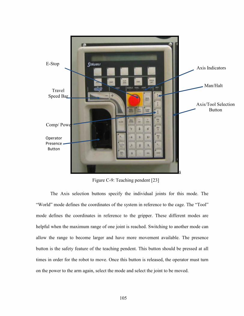
105
ä
Figure C-9: Teaching pendent [23]
The Axis selection buttons specify the individual joints for this mode. The
“World” mode defines the coordinates of the system in reference to the cage. The “Tool”
mode defines the coordinates in reference to the gripper. These different modes are
helpful when the maximum range of one joint is reached. Switching to another mode can
allow the range to become larger and have more movement available. The presence
button is the safety feature of the teaching pendent. This button should be pressed at all
times in order for the robot to move. Once this button is released, the operator must turn
on the power to the arm again, select the mode and select the joint to be moved.
E-Stop
Travel Speed Bar
Axis Indicators
Comp/ Power
Man/Halt
Axis/Tool Selection Button
Operator Presence
Button

106
Programming Commands
The Stäubli robot has a few basic commands that are necessary for its operation.
There are other commands available for more advanced operations. The commands
provided in Table C-1 will allow the completion of this lab and most other basic tasks.
Commands Actions READY Moves the arm to vertical position OPENI Opens the gripper CLOSEI Closes the gripper MOVE #a Moves the robot to point #a along any trajectory MOVES #a Moves the robot to point #a along a straight trajectory
APPRO #a, distance Allows robot to approach point #a by a distance(in mm) along the z-axis DEPARTS distance Moves the robot back from a point along the z-axis DELAY time Specifies a time interval between commands
Table C-1: Commands list [23]
In order to execute these commands, they have to be saved into a file on the
terminal. This is done by using the SEE editor. For example, to create a file for this lab
you must type see box. The editor will notice if there isn’t a file created and will ask you
if you would like to create one.
Defining Points
The ability to define points is one of the Stäubli robots more important features. It
allows the programmer to create a very exact trajectory that is essential to maneuvering
the robotic arm around objects. Defining the points is one of slower processes during the
programming of the robot. They must be manually defined using the teaching pendent.

107
The robot must be moved carefully to one of its desired spots along a trajectory. Once the
robot is in the correct position, the user must type HERE #a and press enter. When the
display asks if you would like to change the point, press enter. The point #a is now
defined in the program ready to be used. This lab will require you to define multiple
points.
Sample Program
Considering the complexity of this exercise, a rough program has been written to
facilitate students through the activity. This is a simple program but does show how the
commands are interrelated. The program needed for the successful completion of this lab
will involve these same commands.
.program pistonball()
ENABLE POWER
SPEED 40
DO READY
MOVE #PARTSAPPO1 ; approach point for picking up parts from platform
MOVE #CONRODAPPO1 ; approach point for picking up conrod
CLOSEI
SPEED 10
MOVE #CONRODAPPO2 ; insert the closed jaws in conrod hole
OPENI
END

108
Procedure
For this exercise, students will use the robot and piston components to perform an
assembly process. Before any programming is started, students should check if the
proper assembly platforms are mounted above the conveyors, and they contain all
necessary components (1 piston, 1 connecting rod, 1 wrist pin, and 1 piston tray).
Additionally, students should make sure the straight gripper fingers are mounted on the
robotic arm. Otherwise, assembly will be quite difficult.
The piston assembly process will involve 4 programming procedures:
1. The robotic arm will be programmed to retrieve a connecting rod from the
part storage platform and place it on the assembly jig
2. The robotic arm will be programmed to retrieve a piston from the part
storage platform and place it on the assembly jig, with the wrist pin holes
aligned properly
3. The robotic arm will be programmed to retrieve a wrist pin from the part
storage platform and insert it into the piston and connecting rod
4. The robotic arm will be programmed to pick and place the assembled
piston into the empty pallet located on the conveyor
Exercise 4 - Integrating Inputs/Outputs with the Stäubli Robot Arm
To understand some of the feedback capabilities of the Staubli robot in Cook Hall,
students will use the robot and conveyor to create an integrated material handling system.

109
This activity has been designed so that students will learn how to integrate both the
Staubli robot and the conveyor segments together to form one cohesive industrial
process. In addition to learning the industrial applications of the material handling
system, students will also learn how photoelectric sensors operate, and how they
communicate with the robot to ensure proper assembly. Students will have to apply robot
programming and operation knowledge gained in previous mechatronic lab activities to
be successful and expedient with the operation. Additionally, programs for both the PLC
and the robot completed in earlier labs will be used. Due to the complexity of the
exercise, students must be sure to operate in a safe and intelligent manner to protect the
robot and conveyor along with themselves.
Background
The Staubli robot is capable of input and output operations through terminal
blocks located in its control cabinet. In the most basic sense, a pushbutton can be
connected to the input terminal block of the robot to start an operation. Similarly, a light
can be connected to the output terminal block of the robot to signal an operation is
completed. In this lab, a photoelectric sensor will be used. The sensor operates by
emitting a beam of light, and measuring how much light returns. If an object is close,
enough light will be reflected back to the sensor to overcome some predefined threshold
and the sensor will activate an output signal. When this signal is connected to the robot, a
process can be instituted that will ensure proper part placement.

110
Programming the Photoelectric Sensor
To program the photoelectric sensor, first turn on power to the robot so that the
sensor is energized. It will emit a red light beam from the LED. To program the sensor’s
“off” setting (return of “false” to the robot), clear objects from the beam or place the
desired object at a distance where a return of “false” would still be desired. Push the
“set” button on the sensor controller. Now position the object where a “true” return is
desired, and press the set button again. The sensor will set the true/false threshold to be
the average of the two reflectivities. It is important to note that if the sensor returns a
reflectivity of 9999 while the first point is being set, the calibration will not work. The
settings will still be recorded, but likely will not work. The syntax for implementing the
sensor into V+ code is as follows:
1 if SIG (10xx) < 0 then (operation)
where xx is the sensor number, ranging from 1 to 12.
Figure C-10: Sensor assembly/ sensor controller [23]
sensor cable output cable
“set” button
scroll buttons
“mode” button

111
System Integration
The Staubli robot will be integrated with the conveyor system to create a
automotive piston assembly system. In this system, two pistons will be assembled and
placed on a tool pallet that will travel along a conveyor system. To accomplish this goal,
the conveyor system from Task 2 will be utilized. Two outputs from the Staubli will be
connected to two inputs of PLC2, and two inputs from the Staubli will be connected to
two outputs of PLC2 as shown below.
Figure C-11: Interconnection diagram between Staubli robot and PLC2 [23]
The program that controls the Staubli will send signals to PLC2 to control the
operation of the conveyor system. It will utilize the inputs from the conveyor system to
ensure the tool pallet is in its proper location. The program to assemble the pistons will
be the same as in Task 3, with some slight modifications. The program to control the
PLCs will be the same as in Task 2, with some slight modifications. Before any
programming is started, students should check if the proper assembly platforms are
mounted above the conveyors, and they contain all necessary components (2 pistons, 2
connecting rods, 2 wrist pins, and 1 piston tray). Additionally, students should make
sure the straight gripper fingers are mounted on the robotic arm. Otherwise, assembly
will be quite difficult.
Staubli PLC2

112
Procedure
1. The photoelectric sensor located underneath the piston assembly jig will
be programmed to detect the alignment of the aluminum wrist pin
2. The Staubli will send a signal to PLC2 to start moving the tray down the
conveyor
3. The robotic arm will be programmed to retrieve a connecting rod from the
part storage platform and place it on the assembly jig
4. The robotic arm will be programmed to retrieve a piston from the part
storage platform and place it on the assembly jig, with the wrist pin holes
aligned properly
5. The robotic arm will be programmed to retrieve a wrist pin from the part
storage platform and insert it into the piston and connecting rod
6. The program will check to ensure the photoelectric sensor detects the wrist
pin
7. The robotic arm will be programmed to pick and place the assembled
piston into the empty pallet located on the conveyor
8. Once two completed pistons have been loaded onto the pallet, the Staubli
will send another signal to PLC2 to move the pallet down the conveyor to
the original starting location.

113
Exercise 5 - Coulomb’s Torsional Pendulum and a Swinging
Pendulum – Similarities and Differences
The behavior of two different types of pendulum will be observed and oscillatory
motion of both the torsional and swinging pendulum laboratory fixtures will be
characterized. Quantification of the torsional pendulum’s motion is accomplished
through the implementation of a Hall Effect sensor while swinging pendulum’s motion is
characterized by an accelerometer.
Background
Fundamentally, the function of a clock is to transform a predictable signal into
some standard unit of time. In pendulum clocks, the position signal of the pendulum is
converted into seconds, hours and minutes. A typical pendulum clock is shown in Figure
C-12. Pendulum motion is predicable and consistent for long periods of time when the
effects of friction are minimized. The second, minute and hour signals are extracted from
the pendulum motion through a series of gears.
The swinging pendulum is the typical pendulum that is present in grandfather and
wall clocks. In contrast, a torsional pendulum is used in anniversary clocks. It represents
a mass hung by a short chord and rotates along the vertical axis. The period of the
torsional pendulum is much longer than that of a swinging pendulum; therefore, the
anniversary clocks will sometimes be called 400 day clocks because some of those clocks
can last 400 days without needing to be wound. In this experiment, the student will study

114
the governing equations of motion by using different laboratory data acquisition
equipment. For the swinging pendulum, the acceleration of the bob will be measured by
an accelerometer; the position and velocity of the bob will be obtained through
mathematical manipulation of the acceleration signal. The torsional pendulum utilizes a
Hall-Effect sensor to determine the rotational position of suspended mass. For this case,
the student shall manipulate the position data to obtain the corresponding acceleration
and velocity. Figure C-12 shows a general assembly for each pendulum.
Figure C-12: Torsional and swinging pendulum [23]
Theoretical Background
Second Order Mechanical Systems
The following analysis of a pendulum first requires an understanding of some
characteristics of second order mechanical systems. Second order systems are systems
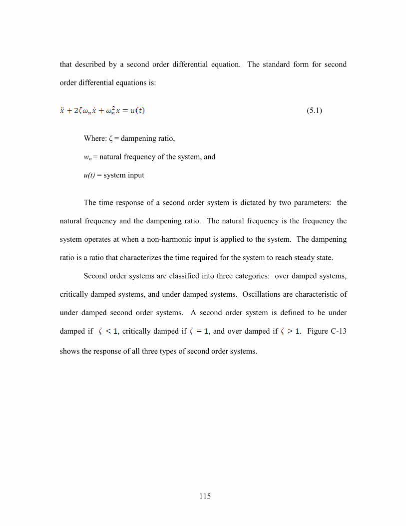
115
that described by a second order differential equation. The standard form for second
order differential equations is:
(5.1)
Where: ζ = dampening ratio,
wn = natural frequency of the system, and
u(t) = system input
The time response of a second order system is dictated by two parameters: the
natural frequency and the dampening ratio. The natural frequency is the frequency the
system operates at when a non-harmonic input is applied to the system. The dampening
ratio is a ratio that characterizes the time required for the system to reach steady state.
Second order systems are classified into three categories: over damped systems,
critically damped systems, and under damped systems. Oscillations are characteristic of
under damped second order systems. A second order system is defined to be under
damped if , critically damped if , and over damped if . Figure C-13
shows the response of all three types of second order systems.

116
0 1 2 3 4 5 6 7 8 9 100
0.2
0.4
0.6
0.8
1
1.2
1.4
1.6
1.8
Time (sec)
Signal
ζ < 1
0 1 2 3 4 5 6 7 8 9 100
0.2
0.4
0.6
0.8
1
1.2
1.4
1.6
1.8
Time (sec)
Signal
ζ = 1
0 1 2 3 4 5 6 7 8 9 100
0.2
0.4
0.6
0.8
1
1.2
1.4
1.6
1.8
Time (sec)
Signal
ζ > 1
Figure C-13: Second order systems: (a) underdamped, (b) critically damped, (c)
overdamped systems vary in behavior due to varying values of ζ [23]
Point Mass Pendulum Analysis
The characteristics of pendulum motion are affected by pendulum geometry. A
simple pendulum is a concentrated point mass connected by a rigid mass less support to a
pivot point, as shown in Figure C-14. When the pendulum is assumed to be a simple
pendulum, only the pendulum mass affects the characteristics of the harmonic motion.
(a) (b)
(c)

117
This type of analysis is called point mass pendulum analysis and though it does not
precisely describe the motion of a real pendulum, it does give a good approximation of
pendulum motion.
Figure C-14: Simple pendulum (a) parameters and (b) free body diagram [23]
The pendulum’s motion is constrained to only degree of freedom, and therefore is
described as a first order system. Given the inputs into the system, the pendulums motion
can be completely defined by an ordinary differential equation of the form
(5.2)
The free body diagram of this motion is shown in Figure C-14. From this figure,
the equation of motion is obtained by summing forces in the tangential direction:
(5.3)
θ
(a) (b)
θ l

118
Where .
Equation 4.3 simplifies to:
(5.4)
Comparing Equation 5.1 with Equation 5.4, it can be seen that the frequency of
oscillation of the pendulum is , and is independent of the mass of the pendulum.
The torque of the pendulum is given as:
(5.5)
Here is the angular acceleration, and is the mass moment of inertia. The mass
moment of inertia of the pendulum is calculated as:
(5.6)
Experimental setup
This experiment contains two different experimental setups for which properties
will be determined. Each setup has a unique pendulum with either a 8 inch (20.3 cm) or
10 inch (25.4 cm) pendulum arm and a .5 pound (0.23 kg) or 1.5 pound (0.68 kg)
pendulum weight. Figure C-15 shows the experimental setup of both the torsional and
swinging pendulum apparatus.

119
Figure C-15: Overall experimental set up [23]
Figures C-16 and C-17 detail the location of the accelerometer for the swinging
pendulum and the location of the Hall Effect sensor for the torsional pendulum.
Figure C-16: Detail of swinging pendulum accelerometer placement [23]
Pendulum
Accelerometer
Pendulum Stand (2)
Protractor (3)
Torsional Pendulum Swinging
Pendulum
Power Supply
Hall Effect
Constant Current supply

120
The swinging pendulum experimental setup consists of a pendulum (1) supported
by a pendulum stand (2), a protractor (3), and an accelerometer (4). In this configuration,
the accelerometer is used to measure the tangential acceleration of the free swinging
pendulum. The protractor is used to determine the angle of the pendulum.
Figure C-17: Torsional pendulum in proximity of Hall Effect sensor [23]
The torsional pendulum setup consists of a stand which serves to support the bob
and allow for mounting of the Hall Effect sensor. The Hall Effect sensor is utilized in
conjunction with a 3 V power supply and a specific Hall Effect circuit. (Diagram
provided in section D)
Power Supply
Hall Effect Circuit
Torsional Pendulum
Hall Effect Sensor

121
Sensors
Accelerometer Details
The accelerometers used in this lab will be the PCB Piezotronics shear
accelerometer model number 333B30. The internal components of the shear
accelerometer with the piezo-electric crystal are shown in Figure C-18. A shear
accelerometer works by having a mass attached to a piezo-electric crystal and when the
accelerometer is accelerated, the mass puts a shear strain on the crystal. This shear strain
is what the accelerometer is actually measuring.
Figure C-18: Internal Components of a shear type piezo-electric accelerometer [23]
This particular accelerometer has an arrow indicating the direction the
accelerometer measures acceleration. In the case of the torsional pendulum, the radius of
rotation is needed to convert linear acceleration to rotational acceleration.
Hall-Effect Sensor Details
Hall-Effect sensors are commonly used in automobiles to time ignition or used to
measure the engine speed which is displayed on a tachometer. A Hall-Effect sensor is a
proximity sensor that uses the change in the magnetic flux to alter the output signal. A

122
magnet is placed on the back side of the sensor which provides the magnetic flux that the
sensor detects. If the north side of the magnet is facing the sensor, the output will be high
at steady state and low when there is a change in the magnetic flux due to the proximity
of a ferrous material. Therefore, it is typical for the south end of the magnet to be facing
the sensor so that at steady state, the output will be low, and when a ferrous material
changes the magnetic flux, the output will be high. The Hall-Effect sensor’s pins are
schematically presented in Figure C-19. When the writing on the sensor can be seen, the
pin layout matches the one above.
Figure C-19: Hall-Effect sensor internal schematic and wiring schematic [23]

123
The Hall Effect sensor signal should resemble the data presented in Figure C-20
below.
Figure C-20: Sample Hall Effect sensor signal over a time period of 0.5 seconds [23]
Each distinct peak nearing the 0.01 volt mark represents a tooth passing through
the sensor’s magnetic field. The rotations per minute of the gear can then be extracted
from the peak/second value if the number of teeth on the gear is known.
Procedure
The procedure consists of mounting the pendulums to the stand and putting the
sensors in place. The circuitry for the Hall-Effect sensor will need to be constructed per
the provided diagram and positioned in a manner in which the gap between the torsional
pendulum and the Hall Effect sensor is small enough for the sensor to output the data
correctly. All parts needed for this experiment are listed in Table C-2.

124
Parts List
2 Accelerometer
1 Swinging pendulum
1 Torsional pendulum
1 5.6kΩ resistor
1 10nF capacitor
1 Hall Effect sensor Table C-2: Parts list [23]
Experimental Procedure for Torsional Pendulum Analysis
1. Connect the torsional pendulum to the test stand. Assure that the
pendulum is secured and the Hall Effect sensor is in an adequate position
to measure data.
2. Ensure that the Hall Effect circuit is set up and connected correctly to both
the power supply and the sensor.
3. Turn the power supply on and set it to 3 volts.
4. Wind the pendulum 3-5 full rotations in either direction. Release the
pendulum and, using the DAQ, record at least one full oscillation.
5. Calculate the angle per tooth on the gear to which will be used to
determine the angular displacement.
6. Transfer data to Excel. Integrate the data from the accelerometer to go
from acceleration to velocity to displacement. Then differentiate the data
from the magnetic variable reluctance sensor to go from displacement to
velocity to acceleration. Compare the two results.

125
Experimental Procedure for Swinging Pendulum Analysis
1. Connect the swinging pendulum to the test stand and mount the rotational
potentiometer to the swinging joint.
2. Turn on the constant current PCB amplifier.
3. Rotate the pendulum to about 45º and release. Using the DAQ, record a
minimum of five full oscillations.
4. Transfer data to Excel. Integrate the data from the accelerometer to obtain
velocity and displacement. Compare the two results with those of the
torsional pendulum.
Exercise 6 - Vibration Modes of a Chime Rod
The vibration behavior of a mechanical clock chime rod will be measured using
an impact hammer with accelerometers. To supplement this study, the acoustics of the
chime rod will also be recorded using a microphone attached to a computer workstation.
The recorded data will be analyzed with Fast Fourier Transform (FFT) to identify the
operating frequencies. The chime rod will be tested in a small semi-anechoic chamber.
Background
Chime rods, see Figure C-21, are used in time keeping mechanisms and offer a
precise musical note which can be used to sound a melody. The striking hammer hits the
chime rod to produce vibrations with frequencies that are dependent on the diameter and
length of the rod.

126
Figure C-21: Wind chime configuration [23]
System Instrumentation
An impact hammer (Figure C-22) is a hand held device used to strike the chime
rod in this experiment. Impact hammers are used to determine system response to
impacts of varying amplitude and duration. A hammer with a force transducer in its head
is paired with an accelerometer on the chime rod. It is used to compare impact and
response. Some key components of the impact hammer are the force and pulse duration.
Different tips can be used to vary the force and response times. The hard tips are used to
measure response at the highest frequencies. Additional masses can attach to the back of
the hammer head to increase the excitation force.

127
Figure C-22: Impact hammer [23]
Accelerometers (Figure C-23) are sensors used to measure, display, and analyze vibration
in conjunction with a data acquisition system. Three main factors must be considered
when selecting accelerometers: amplitude range, frequency range and ambient
conditions. To minimize frequency response errors, the cables attached to the
accelerometer must be securely attached to the chime rod to relive cable strain. This
helps keep the accuracy of the readings as high as possible.

128
Figure C-23: Accelerometer [23]
A microphone, refer to Figure C-24, is a device made to capture waves and
convert them into an electrical signal. The most common microphone uses a thin
membrane that vibrates in response to sound pressure. These vibrations are turned into
an electrical signal, which can be recorded to determine the frequency.
Figure C-24 Microphone used in experiment [23]
Fast Fourier Transform (FFT)
FFT is a method used to calculate the discrete Fourier Transform (DFT). It is an
efficient method that uses algorithms in digital signal processing applications. Using this
function in conjunction with MATLAB allows spectrum analysis to be conducted on the
sound wave recorded using the microphone. The frequency can also be determined using
this function.

129
MATLAB Code
%This code is used to perform a spectral analysis on a wav file that is recorded in
Sound Recorded using a microphone.
clc
clear all
[x Fs nbits]=wavread('chime.wav'); %Insert WAV file
time=length(x)/Fs; %2 steps to create time vector
t=linspace(0,time,length(x));
%THIS PIECE OF CODE IS FROM MATHWORKS. IT CAN BE FOUND AT:
http://www.mathworks.com/support/tech-notes/1700/1702.html
% Use next highest power of 2 greater than or equal to length(x) to calculate FFT.
nfft= 2^(nextpow2(length(x)));
% Take fft, padding with zeros so that length(fftx) is equal to nfft
fftx = fft(x,nfft);
% Calculate the number of unique points
NumUniquePts = ceil((nfft+1)/2);
% FFT is symmetric, throw away second half
fftx = fftx(1:NumUniquePts);

130
% Take the magnitude of fft of x and scale the fft so that it is not a function of
%the length of x
mx = abs(fftx)/length(x);
% Take the square of the magnitude of fft of x.
mx = mx.^2;
% Since we dropped half the FFT, we multiply mx by 2 to keep the same energy.
% The DC component and Nyquist component, if it exists, are unique and should
not be multiplied by 2.
if rem(nfft, 2) % odd nfft excludes Nyquist point
mx(2:end) = mx(2:end)*2;
else
mx(2:end -1) = mx(2:end -1)*2;
end
% This is an evenly spaced frequency vector with NumUniquePts points.
f = (0:NumUniquePts-1)*Fs/nfft;
% Generate the plot, title and labels.
figure(1)
subplot(4,1,1)
plot(t,x)
title('Recorded Wave File')

131
xlabel('Time (s)')
ylabel('Amplitude')
subplot(4,1,2)
plot(f,mx)
ylabel('Spectral Analysis')
xlabel('Frequency (Hz)')
subplot(2,1,2)
plot(f,mx)
axis([10000 11500 0 .00000000000001])
ylabel('Spectral Analysis')
xlabel('Frequency (Hz)')

132
Chime Rods
Figure C-25: Chime rods [23]
Dimensions of these rods are given in the Table C-3:
L D d
Rod 1 15.1 0.963 0.865 Rod 2 13.0 0.978 0.872 Rod 3 12.3 0.972 0.873 Rod 4 11.6 0.973 0.878 Rod 5 10.5 0.966 0.870
Table C-3: dimensions in inches for the chime rods [23]
where is L is the length, D and d are the external and internal diameter
respectively.
1 2
3 4
5

133
Vibrations
Vibration refers to mechanical oscillations about an equilibrium point. In this
experiment, free vibration is studied. Free vibration is a type of vibration that occurs
when an object is impacted with an initial force and then allowed to vibrate freely. The
object will produce vibrations until it damps to zero. Objects usually vibrate at their
natural frequency. See Figure C-25 for an example of the free vibration of a chime rod;
the peak is the natural frequency of the system.
Figure C-26: Frequency response of a chime rod in free vibration [23]
Procedure—Acoustics Experiment
1. Hang chime rod on the rear hook inside semi-anechoic chamber.
2. Place the microphone on the stand.
3. Connect the microphone to input 1 on Audio Buddy pre-amp box.

134
Figure C-27: Audio amplifier [23]
4. Connect the red cord from output 1 on Audio Buddy to the computer
(microphone input).
5. Set microphone inside semi-anechoic chamber as close to the chime rod as
possible without touching it.
6. Open Sound Recorder from Windows start menu.
7. Press Record and strike the chime rod.
Figure C-28: set up for acoustic experiment [23]

135
8. Press Stop after collecting sound data.
9. Save Sound Recorder file as chime.wav in the MATLAB folder.
10. Open wavanal.m file in MATLAB.
11. Run the program and observe the resulting graphs of the spectrum analysis
and frequency of the chime rod.
12. Repeat experiment using a different chime rod. Observe any differences
in the spectrum analysis and frequency graphs.
Procedure—Vibration Experiment
1. Install accelerometer (100mV/g) on chime rod. Hang chime rod on the
rear hook inside semi-anechoic chamber.
Figure C-29: Rod with accelerometer in the chamber [23]
2. Connect the accelerometer cable to channel 2 on SigLab.

136
3. Connect the impact hammer cable to channel 1 on SigLab.
Figure C-30: Connections at Siglab [23]
4. Type “sigdemo” on the command window of MatLab.
5. Press VNA (Virtual Network Analyzer) button in Siglab.
6. Open MechatronicsLab.vna file in SigLab (parameters for this experiment
are saved in this file).
7. Hit “AVG” and strike chime rod using impact hammer. Observe for
changes in the graphs.
8. Hit “STOP”.
9. Copy the plots (impulse response from the hammer and FFT response
from the accelerometer) or export data to be analyzed later.
10. Detach the accelerometer from the chime rod and install it on the next rod
to be tested. Repeat procedures 7-9 until all the 5 rods have been tested.

137
Figure C-31: Set up for vibration experiment [23]
Exercise 7 - Electronic Dice Circuit
Light emitting diodes (LED’s) will be used to create an electronic dice. The
LED’s will be powered by a 4017 decade counter with a clock pulse coming from a 555
timer in astable mode. A toggle switch will control when the dice is effectively “rolling”
and freeze the output state. This circuit uses a high frequency clock pulse so that the
output of the decade counter can not be controlled, creating a random number generator.
This random number lights up the LED’s in the appropriate configuration to simulate a
dice.
Background
As electronic designs get bigger and more complex, it becomes difficult to build
the complete circuit. An Integrated Circuit (IC) has many transistors inside it that are

138
connected together to form a circuit. Metal pins are connected to the circuit and the
circuit is inserted into a piece of plastic or ceramic so that the metal pins are sticking out
the side. These pins allow you to connect other devices to the circuit inside.
When working with a stable circuit, the voltage remains the same. A change in
input voltage results in a change in output voltage, and again the voltage remains constant
until the input is changed. A 555 IC is designed so that when the input changes, the
output goes from 0 to Vcc (Vcc is the voltage of the power supply). The voltage will stay
at Vcc for an amount of time before returning to 0 volts. A graph illustrating this
phenomenon is given in Figure C-32.
.
Figure C-32: A voltage “pulse” [23]
A circuit that varies voltage in this manner continuously is called an oscillator.
An oscillator produces a series of pulses. The output continuously oscillates between 0 to
Vcc. This output is called a clock. You can count the number of pulses to tell how much
time has gone by. A 555 timer can be used to generate continuously varying output
shown in Figure C-33.
.

139
Figure C-33: Timer Output or Clock [23]
Capacitor Details
For example, one type of capacitor is a ceramic disk capacitor, and is shown
below in Figure C-34.
Figure C-34: Capacitor Picture [23]
Capacitors are comprised of two metallic plates separated by a dielectric material.
This creates an electric field which produces certain properties. Certain capacitors may
have markings indicated the polarity of the capacitor. For safety reasons, always insert
the capacitor in the correct orientation if polarity markings are present.
A capacitor can charge and discharge similar to a rechargeable battery. If a 12
volt supply is used to charge a capacitor, it will start with 0 volts and go from 0 volts to
12 volts. A representation a capacitor being charged is shown below in Figure C-35.

140
Figure C-35: Capacitor Charging [23]
The capacitor discharges in a similar manner as it charges. If the capacitor has
been charged to 12 volts and is then shorted thru a resistor, the capacitor will discharge as
shown in Figure C-36. The rate of a capacitor's charging and discharging can be
controlled using resistors.
.
Figure C-36: Capacitor Discharging [23]
555 Timer Details
To create a pulse using a 555 timer it is necessary to connect the timer with
resistors and capacitors into a circuit. The resistor is used to control how fast the
capacitor charges. The bigger the resistance, the longer it takes to charge the capacitor.
The voltage in the capacitor can then be used as an input to another switch. Since the
voltage starts at 0, nothing happens to the second switch. But eventually the capacitor
will charge up to some point where the second switch comes on. The pin-out diagram for
the 555 timer is shown in Figure C-37.

141
Figure C-37: 555 Timer Pinout [23]
The 555 timer operates so that when the voltage supply is connected, the Output
pin goes to Vcc (the positive power supply voltage) and starts charging the capacitor.
When the capacitor voltage gets to 2/3 Vcc (that is Vcc * 2/3) the second switch turns on
which makes the output go to 0 volts.
Pin 2 (Trigger) is the 'on' switch for the pulse. The line over the word Trigger is
representative of the fact that voltage levels are the opposite of what you would normally
expect. To turn the switch on you apply 0 volts to pin 2. Pin 6 is the off switch for the
pulse. We connect the positive side of the capacitor to this pin and the negative side of
the capacitor to ground. When Pin 2 (Trigger) is at Vcc, the 555 holds Pin 7 at 0 volts
(note the inverted voltage). When Pin 2 goes to 0 volts, the 555 stops holding Pin 7 at 0
volts and the capacitor starts charging. The capacitor is charged through a resistor
connected to Vcc. The current starts flowing into the capacitor, and the voltage in the
capacitor starts to increase. Pin 3 is the output (where the actual pulse comes out). The
voltage on this pin starts at 0 volts. When 0 volts is applied to the trigger (Pin 2), the 555
timer puts out Vcc on Pin 3 and holds it at Vcc until Pin 6 reaches 2/3 of Vcc. The 555
pulls the voltage at Pin 3 to ground creating a pulse. The voltage on Pin 7 is also pulled

142
to ground, connecting the capacitor to ground and discharging it. A diagram can be seen
in Figure C-38.
Figure C-38: A stable 555 Timer [23]
In order to make better use of the timer, the speed can be calculated with the
following formulas. See Figure C-38 for descriptions of the variables.
)(**693.0 211 RRCt += (1) 22 **693.0 RCt = (2)
Decade Counter details
A decade counter is an IC given the coded designation of CD4017. There are
many manufacturers of this semiconductor, but they all follow the same pinout as seen in
Figure C-39. The IC uses a clock pulse to cycle through 10 different pins. When a clock
pulse is detected, the IC “counts up” 1 pin. The outputs are in order from Q0-Q9 with
only one being high at the same time. The counter also has a pin that is low from 0 to 4
and high from 5 to 9. This is a decade pin which will create a clock pulse for another

143
counter counting the 10’s digit. Counters can be chained to count very high numbers. The
Reset pin is used to reset the counter back to Q0. This is useful if the circuit does not
require counting to a full ten, since the output of one pin can be used to trigger the Reset
pin. The disable pin prevents any outputs from being on. This IC can handle between 5
and 15 volts.
Figure C-39: 4017 Counter Pinout [23]
Procedure
The procedure for building this circuit will follow the diagram below, but will be
built in sections so that each portion of the circuit can be tested for troubleshooting.

144
Qty Part3 330 Ohm Resistor3 10K Ohm Resistor1 470 Ohm Resistor1 .01uF Capacitor1 .1 uF Capacitor1 555 Timer1 4017 Decade Counter1 Toggle Switch7 LED's
Table C-4: Part list for electronic dice [23]
Figure C-40: Circuit Diagram [23]
555 Oscillator Circuit
1. First place the 555 timer into the breadboard with the number 1 pin in the
top left.
2. Connect Pins 8 and 4 to +5V and connect pin 1 to ground.
3. Connect one side of a 10k Ohm resistor to +5V and the other side to Pin 7.
4. Take another 10k Ohm resistor and connect pin 7 to pin 6.
5. Use a piece of wire to connect pin 6 to pin 2.
6. Place a 0.01uF capacitor between pin 2 and ground.

145
7. The circuit is now complete for the oscillator. Check to see if the circuit is
functioning by connecting the onboard speaker to pin 3 and ground. If you
hear a ringing note, it is functioning.
LED Configuration
8. Take the 7 LED’s and arrange them on the breadboard in a dice
configuration. Make sure the cathode and anode are not on the same rail
and that no LED shares the rail with another. There are three sets of
LED’s in series with the middle LED being alone. See the diagram below.
9. Connect a 330 Ohm resistors to A, B, and D in the diagram below.
10. Connect a 470 Ohm resistor to C.
Figure: C-41: LED Diagram [23]
11. Apply +5V through the resistors to the LED’s and verify that all 7 are lit.
This section of the circuit is complete.

146
4017 Counter Circuit
12. Place the 4017 counter with pin 1 oriented in the top left corner.
13. Connect Pin 16 to +5V.
14. Connect Pin 8 to ground.
15. Connect the 1N4148 signal diodes to pins 1, 2, and 7. Bring the diodes
together on one rail and connect this rail to C on the previous diagram
using the 470 Ohm resistor.
16. Connect the 1N4148 signal diodes to pins 4, 7, and 10. Bring the diodes
together on one rail and connect this rail to D on the previous diagram
using the 330 Ohm resistor.
17. Connect pin 10 to B on the previous diagram using a 330 Ohm Resistor.
18. Connect pin 12 to A on the previous diagram using a 330 Ohm Resistor.
19. Use a 10K Ohm resistor to connect +5V to pin 13.
20. Wire the switch from pin 13 to ground.
21. Connect pin 14 of the 4017 counter to pin 3 of the 555 timer.
22. Connect a 0.1 uF capacitor to between +5V and ground to smooth the
power supply.
23. The circuit is now complete. When powered on, the circuit should light all
7 LED’s until the switch is pressed again. At that point, there should be a
number displayed through the LED configuration.

147
Exercise 8 - Rotation Counter
A circuit that uses an opto-isolator approach will be created that is capable of
counting revolutions. Once per revolution the opto-isolator circuit creates a signal that
causes an integrated circuit to count and display the result on a seven segment display.
Background
This circuit uses four major components that will be covered in the following
sections, light emitting diodes, light dependent resistors, 741 operational amplifiers, and
the 4026 CMOS integrated circuit. The light emitting diode causes the resistance of the
light dependent resistor to drop when the hole is between them. When the resistance
drops, the 741 operational amplifier provides a +9V signal to the 4026 integrated circuit.
This causes the 4026 to count up one and display the number on a seven segment driver.
This effectively counts the number of revolutions.
Light Emitting Diodes
Light emitting diodes (LED) use the flow of electrons through a semiconductor
material to generate a visible light output. The type of material used and the amount of
current flowing determines the brightness of the light. There are two different purposes
for LED’s in this circuit. The first purpose is to create enough light to drop the resistance
of the light dependent resistor. The LED used for this purpose is a 10 mm white LED,
similar to the one pictured in Figure C-42. LED’s require a particular voltage and current,
or the LED will burn out. Generally a larger wavelength requires a smaller voltage drop.

148
Red LED’s require less voltage than Blue LED’s. The white LED used in this experiment
requires roughly 4 volts and 50 mA.
Figure C-42: Light Emitting Diode [23]
The second use of LED’s in this circuit is the seven segment display. Seven
segment displays are an arrangement of seven LED’s that are capable of displaying a
number from 0 to 9. These displays can be either common cathode or common anode.
Common cathode means each LED shares a common ground, while common anode
means they share a common power source. The displays used in this lab are common
cathode and the pinout can be seen in Figure C-43. In Figure C-43, each letter
corresponds to one of the segments, and “DP” refers to the decimal point.

149
Figure C-43: Seven Segment Pinout [23]
Light Dependent Resistors
Light dependent resistors (LDR)’s are resistive elements that are influenced by
the amount of light present. When a LDR is removed from light, its resistance is high.
When a light source is aimed towards the photocell, the resistance drops significantly.
The resistance value can vary. For this circuit, the LDR has a resistance of roughly
10,000 ohms in the dark and 900 ohms when placed into the light. LDR’s are typically
not polarized, so current direction does not matter. A typical light dependent resistor can
be seen in Figure C-34.

150
Figure C-44: Light Dependent Resistor [23]
741 Operational Amplifier
The operational amplifier is capable of taking an input voltage and amplifying it
so that small voltage differences can be used for comparisons or logic circuits. The
maximum voltage that an operational amplifier can reach is determined by its supply
voltage. In this experiment, the 741 operational amplifier will only have +9 volts and
ground, so the max it will produce is 9 volts. The amplifier in this circuit is used as a
comparator. It provides a 9 volt or 0 volt signal based on the voltages present at pins 2
and 3. When pin 2 is higher, the output will be 0 volts. When pin 3 is higher, the output
will be +9 volts. A pinout of the 741 operational amplifier can be seen in Figure C-45. A
voltage output based on the resistance of the light dependent resistor (LDR) and resistor
on pin 2 (R1) can be seen in Figure C-46.

151
Figure C-45: 741 Pin Configuration [23]
Figure C-46: Comparator Output [23]
4026 CMOS Integrated Circuit
The 4026 CMOS integrated circuit provides two functions in one chip. It provides
a decade counter with the ability to count from 0 to 9. The 4026 also simplifies wiring by
converting this number to a format that can be displayed on a seven segment display. A
pinout can be seen in Figure C-47 and the output based on count is shown in Figure C-48.

152
Figure C-47: 4026 Integrated Circuit [23]
The clock input on the 4026 is used for counting. If the disable clock pin is high,
the 4026 pauses counting. The enable display pin must be high or the display will be
blank. Enable out follows the input with a brief delay. The decade pin provides a low
output from 0 to 4 and a high output from 5 to 9. Reset allows the count to be returned to
zero. The not 2 output is high unless the count is 2. Outputs A through F represent the
seven segments of the display.

153
Figure C-48: 4026 Output [23]
Procedure
The procedure for building this circuit will follow the diagrams in Figure C-49
and Figure C-50, but will be built in sections so that each portion of the circuit can be
tested for troubleshooting.
To counter circuit
3K
1K-10K
LDR
9 V
741 Op Amp
1234
5678
LED 5K
5K
330
Figure C-49: Sensor Circuit

154
Figure C-50 Display Circuit [23]
Qty Part8 330 Ohm Resistor1 3K Ohm Resistor1 1K Ohm Resistor1 741 Op Amp1 4026 IC1 7 Segment Display1 LDR1 White LED
Table C-5: Part list for rotation counter [23]
Sensing Circuit
1. First place the 741 amplifier into the breadboard with the number 1 pin in
the top left.
2. Connect Pin 7 to +9V and connect pin 4 to ground.
3. Take the leads coming from the LDR and connect one to +9V and connect
the other to pin 3 of the 741 amplifier. The leads should be black.

155
4. Take a 3k ohm resistor and connect one side to +9V and the other side to
pin 2 of the 741 amplifier.
5. Connect a 330 Ohm resistor to +9V and connect the other end to the
positive lead for the LED. The color of this wire should be red.
6. Connect the ground of the LED to ground. The color of this wire should
be yellow.
7. Time to test the circuit. Place a LED with 330 ohm resistor to pin 6 of the
741 amplifier. Spin the wheel and check to ensure the LED is flashing
when appropriate. If the LED fails to light, increase the resistor to pin 2. If
the LED is always on, decrease the resistor to pin 2. Once the circuit is
verified working, remove the LED and resistor.
Display Circuit
8. First place the 4026 IC into the breadboard with the number 1 pin in the
top left.
9. Connect pins 3 and 16 to +9V. Connect pins 2,8, and 15 to ground.
10. Place the seven segment display onto the breadboard. Follow the diagram
and connect pins as described in Table C-6. Include 330 Ohm resistors in
each connection.

156
4026 Pin Display Pin 6 10 7 9 9 2 10 7 11 1 12 6 13 4
Table C-6: Pin Connections [23]
11. Connect Pin 1 of the 4026 IC to +9V and make sure it counts up one. If
the circuit counts up one, connect pin 1 of the 4026 IC to pin 6 of the 741
op amp.
12. Connect the positive lead for the motor to a 47 Ohm resistor, and the other
side to +5 V. Connect the ground for the motor to ground.
13. The circuit is finished. Give the wheel a spin and watch the counter count
up the total number of spins.

157
REFERENCES
1. Material Handling Institute of America, www.mhia.org/learning/marketresearch,
2009
2. Khan, O., “Current Technological Development and Mechatronics”, proceedings of
the IEEE International Multi-Topic Conference, pp. 111-117, Lahorse University,
Pakistan, December 2001.
3. Merkel, C., and Fisher, D., “A Quick and Easy PLC Learning Experience for
Mechatronics”, Proceedings of the ASEE Annual Conference, pp. 895 – 906,
Chicago, IL, June 2006.
4. Chiou, R., Kwon, Y., Rauniar, S., and Sosa, H., “Internet-based Robotics and
Mechatronics Experiments for Remote Laboratory Development”, Proceedings of the
ASEE Annual Conference, pp. 1363-1379, Honolulu, HI, June 2007.
5. Lee, C., and Park, S., “Sensor-Based Robot Control Laboratory”, Proceedings of the
ASEE Annual Conference, New Orleans, LA, June 1991.
6. Marsico, S., “Incorporating a Flexible Manufacturing System into a Design Course”,
Proceedings of the ASEE Annual Conference, Montreal, Quebec, Canada, June 2002.
7. Erickson, K., “Innovative Experiments for Undergraduate Factory Automation”,
proceedings of the 13th World Congress, International Federation of Automatic
Control, San Francisco, CA, June 1996.

158
8. Stormont, D., and Chen, Y., “Using Mobile Robots for Controls and Mechatronics
Education”, International Journal of Engineering Education, vol. 21, no. 6, pp. 1039-
1042, 2005.
9. Ghone, M., and Wagner, J., “A Multi-Disciplinary Mechatronics Laboratory”,
Proceedings of the ASEE Annual Conference, Nashville, TN, pp. 1607-1614, June
2003.
10. Vermaak, H., and Jordaan, G., “Automated Component-Handling System for
Education and Research in Mechatronics”, Proceedings of IEEE AFRICON
Conference, pp. 4401627, Windhoek, South Africa, September 2007.
11. Bassily, H., Sekhon, R., Butts, D., and Wagner, J., “A Mechatronics Educational
Laboratory – Programmable Logic Controllers and Material Handling Experiments”,
Journal of Mechatronics, vol. 17, no. 9, pp. 480-488, November 2007.
12. Material Handling Institute of America (MHIA), www.mhia.org, 2008.
13. Wagner, J., "Evolving Industry Expectations for Engineers - The Impact of Global
Manufacturing", Proceedings of the ASEE Conference, Charlotte, NC, June 1999.
14. Acar, M., and Parkin, R., “Engineering Education for Mechatronics”, IEEE
Transactions on Industrial Electronics, vol. 43, no. 1, pp. 106-112, February 1996.
15. Krotkov, E., “Robotics Laboratory Exercises”, IEEE Transactions on Education, vol.
39, no. 1, pp. 94-97, February 1996.
16. Ghone, M., Schubert, M., and Wagner, J., “Development of a Mechatronics
Laboratory-Eliminating Barriers to Manufacturing and Control”, IEEE Transactions
on Industrial Electronics, vol. 50, no. 2, pp. 394-397, April 2003.

159
17. Shirley, J., Wagner, J., Collins, R., and Gramopadhye, A., “A Mechatronics (and
Material Handling Systems) Course – Classroom Topics, Laboratory Experiments,
and Project”, Proceedings of the ASEE Annual Conference, Austin, TX, June 2009.
18. Murray, W., and Garbini, J., “Mechatronics Capstone Design Projects at the
University of Washington”, Proceedings of the IEEE/ASME International Conference
on Advanced Intelligent Mechatronics, pp. 598-604, Atlanta, GA, September 1999.
19. Ebert-Uphoff, I., Gardner, J., Murray, W., and Perez, R., “Preparing for the Next
Century: the State of Mechatronics Education”, IEEE/ASME Transactions on
Mechatronics, vol. 5, no. 2, pp. 226-227, June 2000.
20. Du, W., “On Improvement of Graduate Mechatronics Course”, Innovations in
Engineering Education 2005: Mechanical Engineering Education, Mechanical
Engineering Technology Department Heads, vol. 2005, pp. 191-196, Orlando, FL,
November 2005.
21. Thrambouldis, K., “Model-Integrated Mechatronics – Toward a New Paradigm in the
Development of Manufacturing Systems”, IEEE Transactions on Industrial
Informatics, vol. 1, no. 1, pp. 54-61, February 2005.
22. Jammes, F., and Smit, H., “Service-oriented Paradigms in Industrial Automation”,
IEEE Transactions on Industrial Informatics, vol. 1,no. 1, pp. 62-70, February 2005.
23. Wagner, J., “ME 493/693 Laboratory Manual”, V2.0, Department of Mechanical
Engineering, Clemson University, Clemson, SC, August 2009.