the determinants of the labour force participation rate in ... · the determinants of the labour...
TRANSCRIPT

The Determinants of the Labour Force
Participation Rate in Canada, 1968-97:
Evidence from a Panel of Demographic Groups
Mario Fortin University of Shrebrooke
Pierre Fortin University of Quebec at Montreal
May 1998
Paper presented at the annual meetings of the Canadian Economics Association, Ottawa, May 30,1998. This is a work on progress and the findings reported in this paper are preliminary. Do not quotewithout permission from the authors. We would like to thank David Green and Allan Crawford fortheir comments.

Our last year study reveals also that young males behaved slightly differently in the Atlantic region than in the1
rest of the country.
1
1. Introduction
Between 1990 and 1995, five successive years of decline in the Canadian participation rate
pushed it down from 67.5% to 64.8%, a fraction which remained stable thereafter. Because this
sudden and significant decline in the trend participation rate has no precedent, it has become, with
the sustained high level of unemployment, the major fact of Canada’s labour market in the 90s. Since
the sudden occurrence of the decline and its persistence call for diverging explanations, a single cause
is not likely. While abrupt movements naturally leads to suspect cyclical factors, the persistence
generally points toward structural explanations. Given that the 90s have witnessed the most
prolonged cyclical slump in Canada since the 30s, there is no ambiguity as to whether or not the usual
pro-cyclical reaction of the participation rate may have played a role in the decline. Yet, the relative
contribution of cyclical and structural factors are essential to address correctly the issue. If it were
mainly a cyclical decline, then the participation rate could return close to its previous high of 67.5%,
which implies that it remains presently a significant output gap. At the opposite, potential output
would be close to actual output if structural factors explain much of the decline.
This paper disentangles the change in the participation rate according to three types of
factors, that is, cyclical, trend, and social programs. Moreover, since the repartition between these
factors varies with age and sex, we analyze the movements of the labour force along three age groups
(15-24, 25-54 and 55 and over) for both sexes. This exercice is an update and a complement of Fortin
and Fortin (1997) in which we estimated the contribution of these same factors for a panel of five
regions and six demographic groups. Despite that we then found significant statistical differences in
the regional behaviour of females, we will not focus on these regional discrepancies in this study to1
concentrate our attention to the more important differences observed amongst demographic groups.
The concept of generosity we use if the maximum subsidy rate of employment income by unemployment2
insurance. Our calculation show that the Canadian average of this subsidy rate was approximately 31.5% in the 60s, reachedapproximately 2..5 between 1972 and 1975, and was still 1.8 in 1989. Since the last three legislative changes of the 90s,the subsidy rate has fallon to approximately 0.62.
2
Some of the demographic groups we havedefined have received a particular attention recently.
Grignon and Archambault (1998) analyze how structural and cyclical factors explain the decline in
the youth participation rate with a particular emphasis in distinguishing between students and non-
students. Lemieux and Beaudry (1998) analyze more specifically the role of cohort in explaining the
changing trend of females. Our contribution in this literature in twofold. First, by applying the same
model to all demographic groups, we analyze in a consistent way the participation rate. Second, we
put a particular emphasis in the measure of the impact of legislative changes in the unemployment
insurance (UI) program. This emphasis on UI leads us to make three fondamental decisions regarding
the appropriate treatment of this variable.
First, we think it is very important to use a sample that begins in the 60s. As many before have
pointed out, the 1971 reform of UI is the main candidate to explain why the Canadian unemployment
rate has not been declining with respect to the U. S. rate in the 70s despite the fact that the
employment ratio was growing much faster in Canada (See, for example, Card and Riddell, 1993).
Indeed, one of the main prediction of the classical labor supply is that when UI heavily subsidizes
sporadic employment, this will makes some marginally attached workers to move in the labour force
(Fortin, 1984). Following the 1971 reform, a subsidy rate as high as 367% was possible in some
regions of Canada. Subsequent changes somewhat reduced this maximum subsidy rate but it was
mainly in the 90s, with a succession of legislative changes in 1990, 1994 and 1996, that the generosity
of the program was significantly reduced to return closer to the level of generosity seen before the
1971 reform of US. Given that the participation rate reaction of the 90s to UI is just the reverse23
reaction of the 70s, it becomes important that the empirical model is able to explain as well the rise
of the 70s than the fall of the 90s.

The bottom ligne of these elements lies on the simple observation that between 1971 and 1978, the Canadian4
Beveridge curve drifts on the right at a decreasing speed.. Although by no means a proof that the 1971 reform is solelyresponsible for this movement, is is certainly consistent with a gradual response of the participation rate.
3
Second, we do not directly use the generosity of the program but rather an instrument for this
variable. The reason behind this decision lies in the retroaction between the participation rate and the
generosity of the program. One of the characteristics of the UI program is that the maximum duration
of benefits and the qualification condition are dependent on the regional unemployment rate. If for
some reasons the participation rate changes, this implies a response of the unemployment rate which,
in turns, influences the generosity of the program and the explanatory variable. This violates the
assumption of independence between the error terms and the regressors. To avoid a biased measure
of the impact of UI, we calculated an index of the generosity of the program that responds solely to
legislative changes. Finally, our third contribution lies on the explicit recognition that the response
of the participation rate to UI changes may not be immediate. There are empirical elements, already
pointed out namely by Fortin (1994) and by Archambault and Fortin (1997), which strongly suggests
that this could be the case. Thus, we estimate a lag structure for the UI variable in the participation4
rate equation.
The paper is organized as follows. The next section presents a theoretical model of labour
force participation. Data and estimation of a system of equations for six demographic groups are
presented in section 3. The fourth section indicates the implications of the results for a global
participation rate equation and compares with an estimation of a single participation rate equation.
Concluding remarks close the paper in the last section.
2. The theory
We consider an individual who must choose between entering into the labour force, which
may lead to employment or unemployment, or remaining out of it and be inoccupied. The monetary
value of the reservation value of time of the individual i at period t is given by " (J ), where J is anit t t

We must emphasize that d is not the maximum duration of benefits but the maximum number of benefits weeks5
for a minimally qualified person. As in Fortin (1984), the main determinant of the change in the participation rate is themaximum subsidy of employment rate.
4
index of its non-labour income. When deciding to be active, it is uncertain if it will occupy a job or
remain unemployed. The expected payoff from participating is then an average of the income received
while unemployed or employed. In the former case, he must be searching for a job and pay a cost
c, which includes both direct costs and indirect inconvenients related with searching, so that its
satisfaction level is " (J )-c. As to employment, we assume that at period t, all jobs pay an identicalit t
wage w. However, because of UI, wage is not the only component of remuneration. Given that ant
employee works at least m periods, it is entitled to receive d periods of UI benefits set at a fractiont t
R of the wage. Following Fortin (1984), we define the maximum subsidy rate D as the product oft t
the benefit rate R by the ratio d /m , that is, D = R× d /m . In addition to the labour income w , eacht t t t t t t
period of work thus entitles the worker to UI benefits of a value Dw. By assuming that benefits rightst t
are valued as much as labour income, the total income received for each period of work is then
w (1+D ).t t5
We complete the description of the expected payoff by a description of the probability p(N )t
of beeing employed if someone participates to the labour market. We suppose that N is an index oft
business cycle conditions such that dp(N )/dN > 0. The expected payoff of participating to the labourt t
market is then p(N )w (1+D ) + [1-p(N )][" (J )-c]. Individual i participates to the labour market ift t t t it t
the following inequality is verified :
p(N )w (1+D ) + [1-p(N )][" (J )-c] $ " (J ) (1)t t t t it t it t
The marginal active person on the labour market satisfies equation (1) with equality. If "it*
is the reservation value of time of this marginal person, we then have the equality p(N )w (1+D ) +t t t
[1-p(N )][" (J )-c] = " (J ). With a simple manipulation, one can write :t it t it t* *

5
" (J ) = w (1+D ) + c[1-p(N )]/p(N ) (2)it t t t t t*
As a last step, we analyze the aggregate consequences of these individual decisions. Let us
assume that " follows the marginal continuous distribution f(" ). The cumulative distribution is thenit it
F(" ). Since the labour force A is equal to the number of persons that satisfies equation (1), is is thusit t
equal to F(" ), that is, the cumulative distribution evaluated to the marginally attached person. Theit*
labour force equation is then given by :
A = F(" (J )) = G(w (1+D ) + c[1-p(N )]/p(N ),J ) (3)t it t t t t t t*
Dividing by the population of 15 and over (P ) gives the participation rate a = A /P . Let g(·)t t t t
= G(·)/P . We can then write :t
a = F(" (J )) = g(w (1+D ) + c[1-p(N )]/p(N ),J ) (4)t it t t t t t t*
It is easy to show that a increases with w (1+D ) and with N but decreases with J . Thist t t t t
implies that the participation rate is pro-cyclical and an increasing function of the maximum subsidy
rate of employment income by unemployment insurance. However, the activity rate is negatively
affected by the non-labour income J . These last two predictions are consistent with the modelt
presented in Arnau, Crémieux and Fortin (1998). Finally, the model predicts that the wage
unambiguously raises the participation rate.
Before turning to estimation, some remarks help in translating the theoretical predictions into
real world expected impacts. First, the predicted positive impact of the real wage is not consistent
with respect to the usual ambiguous impact of wages on labour supply. The reason for this difference
lies in the implicit assumption that individuals can work either full time or not at all. Because of these
limitations, the budget constraint is composed of only two points in the expected income/time space.

6
A rise in wage improves the expected payoff from participating while leaving unchanged the
satisfaction level of non-participation. In a less rigid environment in which individuals can choose the
fraction of working time, the positive income effects of a higher wage allows individuals to work a
smaller fraction of their total time. This could be achieved either by working for a shorter time each
period, or by reducing the number of periods working full time. In the second case, the aggregate
consequence would be that the participation rate could fall when the wage rate rises. Since we believe
that this reaction is possible, we make no a priori assumption regarding the impact of wage.
A second remark is in order concerning the minimum wage. It has long been recognized that
the minimum wage has two opposite consequences on labour market participation. Because better
paid jobs raise the expected payoff, more minimally qualified workers may be drawn into the labour
force than would be the case in the absence of a minimum wage. However, these higher wages may
reduce the number of jobs available. Therefore, as the model shows, a lower probability of finding
a job depresses the participation rate. Thus, and despite the fact that the model explicitly takes into
account the wage impact and the employment probability, it is possible that the empirical variables
do not capture the specific impact of the minimum wage on participation. Since this impact depends
of the effect of the minimum wage at a given distribution of wages, we add as an additional variable
the ratio of the minimum wage to average wage. The theoretical participation rate equation is then
of the form :
a = f(N , w , wmin /w , D , J ) (5)it t t t t t t
with an expected positive impact of N and D , and a negative influence expected for the non-labourt t
income J . As to w and wmin /w , they can be of either sign.t t t t

7
3. The empirical model and the data set
The participation rate of the entire working age population is an average of the participation
rate of many demographic groups which sometimes have very different behaviour. This is easily
illustrated by the fact that the trend in the participation rates of males and females have been of
opposite signs over the last thirty years. This has for consequence that when group shares are
changing, the aggregate pamameters becomes unstable and, because of this, may lead ot unconsistent
estimates. To circumvent the problem, we estimate the parameters for six demographic group, that
is, male and female for the age groups 15-24, 25-54 and 55 and over. From these estimates, we
recover the global equation by simply calculating the group average for each coefficient. Since the
participation rate in level is non-stationnary, the following system of equations was estimated in first
difference :
)log(a ) = $i + $i )log(N ) + $i )log(w ) + $i )log(wmin /w ) + $i )log(SAB /wmin )it 0 1 t 2 t 3 t t 4 t t
+ $ )log(UIG ) + $ )T + u i = 1, þ, 6 (5)i5 t 6 t it, ,
The left hand variable is the logarithmic change in the participation rate of group i. All right
hand variables, with the sole exception of the time trend, are also expressed in logarithmic differences.
The first variable is a cyclical indicator of the probability of finding a job. A natural choice for this
cyclical indicator is the employment/population ratio(e ). However, because some of the movementsit
in e are the results of changes in a , using directly e as a regressor in the equation would create ait it it
simultaneity bias. More precisely, the coefficient of e would over-estimate the true cyclicalit
sensitivity of the participation rate. In order to avoid this problem, we could as in Fortin and Fortin
(1997), use a two stage least square to estimate an instrument for e . We rather preferred the simplerit.
method of instrumenting the employment/population ratio with the ratio of the help-wanted index
(HWI) to the population of 15 and over. Archambault and Fortin (1997) showed that an index of the
vacancy rate based on the HWI reacts strongly and fastly to cyclical shocks but is unsensitive to

The conclusion was based on the fact that in a VAR, the variance decomposition of the HWI into cyclical,6
structural and participation rate finds a contribution of cyclical shocks close to 100% at any time horizon. We further checkedthe appropriateness of this instrument by regressing the logarithmic change in the employment population ratio on thelogarithmic change of the instrument and on the logarithmic change of the real per capita GDP over the period 1967-1997and only the first variable stands out as a significant regressor. Morevoer, the adjusted R of this regression (0.735) is lower2
than when the employment population ratio is explained solely by the instrument (0.742).
8
shocks to the particpation rate, which makes it a good instrument for capturing the cyclical6
movements in the probability of finding a job. We divided the HWI by the population to correct for
the growing size of the labour force.
The second variable is the logarithmic change in the real consumption wage, that is, the
nominal wage divided by the consumer price index. The third variable is the logarithmic difference
in the relative minimum wage, which is defined as the ratio of the minimum real wage to the average
real wage. The fourth variable is the logarithmic change in the relative social assistance benefit
(SAB), which is defined as the ratio between, on one hand, total benefits in real value divided by the
number of beneficiaries and, on the other hand, the real minimum wage. As Arnaud, Crémieux and
Fortin (1998) show, the real social assistance benefits, which is the minimum out of work income,
influences working incentives because it reduces the marginal net income from working. Since social
assistance benefits are mainly used by low skilled workers whose main labour market alternative is
non-specialized work paid a the minimum wage, this ratio crude measure of the potential impact
SAB can have on labour market participation is the logarithmic difference between real social
assistance and the minimum wage.
The fifth variable captures the impact of UI benefits on the participation rate. We use
log(1+D) because in the theoretical model, employment income is defined as w×(1+D ) so that thist t t
product is additive in the logarithm. The UI subsidy rate is defined as the average of the subsidy rate
in all regions of Canada. Moreover, to eliminate the retroaction between the unemployment rate and
the index of the generosity of UI, we use a standardized index calculated not on the actual
unemployment rate but under the hypothesis that the unemployment rate has remained constant to

The UI variable used in the model is )UIG = -0.09057×)(1+D ) + 1.14718×)(1+D ) + 0.18548×)(1+D ) -7t t-1 t-2
0.24021×)(1+D ). We constraint the sum of the weights to be one to preserve the interpretation that the coefficient is ant-3
elasticity. In subsequent steps of this study, we will explore more thorouhgly the possibility of using different lag structuresin each equation.
9
its sample mean. Thias implies that the variable is an instrument that reflects solely changes in
legislation. Finally, because the labour supply reaction to UI changes is likely to be progressive, we
used a moving average of current and lagged values of (1+D). The length of this MA has been chosent
to maximize the adjusted R and to minimize the information criteria. Finally, the last variable is a2
simple time trend. Since the model is estimated in first difference, the trend growth rate of the
participation rate is captured by the constant. The time trend allows this growth rate to change
progressively. Because the variables are in log rate of change, each coefficient has the dimension of
an elasticity.
The data set is composed of annual observations covering the period from 1966 to 1997 for
all the variables with two exceptions. The data for the social assistance benefits were available only
from 1968 to 1996. As to the index of UI generosity, it was easy to calculate its value back to the
beginning of the sixties (See appendix). Because the series are in first difference, the estimation is
made on 28 annual data from 1969 to 1996 for 6 groups, that is, a total of 168 observations. We
estimated the system of equations by the method of Zellner’s Seemingly Unrelated Regression (SUR).
Since we use the same set of regressors in each equation, SUR estimates are identical to OLS
estimates. Yet, SUR estimates are nevertheless more efficient thant OLS. By taking account of the
correlation of the errors between equations, SUR provides smaller estimated variances and more
powerful tests. We used the fact that the estimates were identical to OLS to explore the impact of
various specifications of the lag length of (1+D ) in each equation. It became rapidly obvious, as wet
will show in a short time, that UI has a significant impact particularly for young people. The
information criteria from the OLS equation for young males and females suggest to keep three lags
of (1+D) in addition to the current value. Thus we retained the OLS estimates of the three lags of
(1+D) to calculate the MA. Appendix 1 gives the source of all data.7

10
3. The estimation results
The first set of results are those of the unconstrained SUR, reported in table 1. These
equations have been submitted to many tests to detect any symptom of misspecification. The LM test
with two lags do not detect any significant autocorrelations of the residuals. The RESET test do not
allow to reject the null hypothesis that one or two fitted terms have no impact on the dependent
variable. The stability of the parameters was checked by the means of Chow tests with a breakpoint
in 1981 and by looking at recursive estimates. Once again, ne problems were detected.
Table 1Unconstrained SUR estimates
Variables 15-24 (M) 15-24 (F) 25-54 (M) 25-54 (F) 55+ (M) 55+(F)
Constant 0.0092* 0.0311 0.0018 0.0593 -0.0034 0.0322(0.0054) (0.0069) (0.0015) (0.0044) (0.0096) (0.0145)
^^ ^^ ^
Nt0.0654 0.0423 0.0130 0.0099* -0.0021 0.0034^^
(0.0074) (0.0093) (0.0021) (0.0059) (0.0130) (0.0196)
^^ ^^
wt-0.1042 -0.2562 -0.0603 -0.2053 -0.1355 -0.3288(0.0911) (0.1143) (0.0253) (0.0730) (0.1599) (0.2408)
^ ^ ^^
wmin /wt t-0.1618 -0.1587 -0.0058 -0.1556 -0.1241 0.1508^^
(0.0553) (0.0693) (0.0154) (0.0443) (-0.1197) (0.1460)
^ ^^
SABt0.0146 -0.0342 -0.0112 -0.1041 -0.1197* -0.1709*
(0.0371) (0.0465) (0.0103) (0.0297) (0.0650) (0.0979)
^^
UIGt0.0703 0.0571 -0.0017 0.0148 0.0126 -0.0964^^
(0.0167) (0.0209 (0.0046) (0.0133) (0.0292) (0.0440)
^^ ^
Tt-0.0005* -0.0013 -0.00015 -0.0019 -0.0007 -0.0017(0.0003) (0.0003) (0.00007) (0.0002) (0.0005) (0.0007)
^^ ^ ^^ ^
R2 0.8632 0.7892 0.6866 0.8534 0.1680 0.2726
Adj. R 0.8241 0.7289 0.5970 0.8116 -0.0698 0.06482
S. E. 0.0082 0.0103 0.0023 0.0066 0.0144 0.0217
D. W. 1.8023 2.2407 2.5210 2.0759 2.6336 3.0806
The symbols *, and indicate that the coefficient is significant at the 10%, 5% and 1% level respectively. Standard deviations are between parenthesis. ̂ ̂ ^

11
The R of the model varies considerably in the different equations. The model performs very2
poorly in explaining the time series behaviour of the participation rate of both males and females of
55 and over. This indicates that the changes in the participation rate for older people is not sensitive
to the business cycle and there is no influence of social programs at the usual statistical level.
However, the equations explain more than 80% of the variations in the participation rate of males 15-
24 and of females 25-54 and close to 80% for females 15-24. This fraction is a bit smaller for male
25-54 but reaches nevertheless 68%. Given that the estimation is in first difference and that the lagged
value of the dependent variable do not appear in the specification, this denotes a high explanatory
power of the model. We now turn our attention to the impact of each variable.
i. Cyclical variable
The model shows large differences in the cyclical sensitivity of the participation rate in the
various demographic groups. The greatest sensitivity is observed for young males, with an elasticity
of the participation rate to N of 6,5% while it is only 1,3%, that is, five times smaller in the age groupt
25-54. As to women, the elasticity is about 2/3 the elasticity observed in males for the same age
group, and the cyclical variable is significant only at the 10% level in the equation for women 25-54.
As for older people, the model do not detect any statistically significant response of the participation
rate to cyclical changes.
ii. Real wage
The coefficient of the real wage is negative in all six equations and is significant at the 1%
level for females 25-54 while it is significant at the 5% level in the equation for males 25-54 and for
females 15-24. However, since the minimum wage is expressed in log differences with respect to the
real wage, the correct impact of the real wage is measured by the difference between the coeffcient

Since the estimated equation is involves the expression $i )log(w ) + $i )log(wmin /w ), this can be written82 t 3 t t
as $i )log(w ) + $i )log(wmin ) - $i )log(w ) = ($i -$i )log(w ) + $i )log(wmin ).2 t 3 t 3 t 2 3 t 3 t
12
of these two variables. The null hypothesis that the real wage has no impact in all equations has a P8 2
of 6.304990 and a marginal probability of 0.504623. Thus, one cannot reject the null hypothesis that
the real wage plays no role in explaining the participation rate for all demographic groups.
iii. Relative minimum wage
Since the minimum wage divides the social assistance benefits, its impact is measured as the
difference between the third and the fourth coefficient in each equation. This variable has a negative
impact on the participation rate for the youth, for femal 25-54 and for males 55+. Its impact of the
participation rate is significantly lower than zero at the 1% level for young males and at the 5% level
for young females. It is significantly positive at the marginal level of 1.3% for female workers 55+.
iv. Relative social assistance benefits
The relative social assistance benefits has a negative impact for five groups. However, the
usual 5% significance level is attained only for women 25-54. For both men and women over 55, the
impact is significant at the 10% level and the largest coefficient (-0.17) is found for women over 55.
v. Unemployment insurance generosity
For both males and females 15-24, this variable has a similar positive impact (0.07 for males
and 0.057 for females) that is significant at the 1% level. The model also detects a significant impact
at the 5% level for females over 55 but the sign is negative. As to males and females 25-54, the model
does not detect a significant reaction to the UI generosity.
vi. Time trend
The trend growth rate of a is captured by the constant while the time trend indicates if thet
trend growth rate is declining of increasing. For females of all age, the growth rate was initially
13
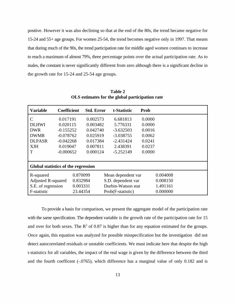
positive. However it was also declining so that at the end of the 80s, the trend became negative for
15-24 and 55+ age groups. For women 25-54, the trend becomes negative only in 1997. That means
that during much of the 90s, the trend participation rate for middle aged women continues to increase
to reach a maximum of almost 79%, three percentage points over the actual participation rate. As to
males, the constant is never significantly different from zero although there is a significant decline in
the growth rate for 15-24 and 25-54 age groups.
Table 2OLS estimates for the global participation rate
Variable Coefficient Std. Error t-Statistic Prob
C 0.017191 0.002573 6.681813 0.0000DLHWI 0.020115 0.003482 5.776331 0.0000DWR -0.155252 0.042740 -3.632503 0.0016DWMR -0.078762 0.025919 -3.038755 0.0062DLPASR -0.042268 0.017384 -2.431424 0.0241XJH 0.019047 0.007811 2.438391 0.0237T -0.000652 0.000124 -5.252149 0.0000
Global statistics of the regression
R-squared 0.870099 Mean dependent var 0.004008Adjusted R-squared 0.832984 S.D. dependent var 0.008150S.E. of regression 0.003331 Durbin-Watson stat 1.491161F-statistic 23.44354 Prob(F-statistic) 0.000000
To provide a basis for comparison, we present the aggregate model of the participation rate
with the same specification. The dependent variable is the growth rate of the participation rate for 15
and over for both sexes. The R of 0.87 is higher than for any equation estimated for the groups.2
Once again, this equation was analyzed for possible misspecification but the investigation did not
detect autocorrelated residuals or unstable coefficients. We must indicate here that despite the high
t-statistics for all variables, the impact of the real wage is given by the difference between the third
and the fourth coefficent (-.0765), which difference has a marginal value of only 0.182 and is

14
therefore not statistically significant. As to the minimum wage, its impact is given by the difference
between the fourth and the fifth coefficient (-0.0365) and is significant only at the 0.11 marginal level
4. Decomposing the participation rate from 1989 to 1997
We can now calculate the contribution of cyclical and structural factors in the falling
participation rate of the 90s. The empirical model explains the changes in the participation rate. We
used the estimated coefficients to calculate the impact of each explanatory variables in the changes
in the participation. Then, we computed recursively how this has affected the level of the participation
rate. The level of all series has been set to be identical to the actual series for the year 1989. Thus,
all subsequent results can be interpreted as the contribution of each variable to the evolution of the
participation rate, if all other variables had kept their 1989 level.
Our first interest is in explaining the global participation rate. There are two ways to calculate
the empirical impact of the variables. The first possibility is to use the estimated impact for each group
to calculate an average for the whole population by using each group’s population share. The second
way is simply to use the global equation. As we discussed previously, the first method is preferable
and was chosen for our first analysis of the global behaviour. Since the equations were estimated up
to 1996, because we did not have tha 1997 data for social assistance benefits, the response for 1997
in an out of sample forecast
The figures 1 and 2 show the estimated response of the global participation rate to the
explanatory variables, calculated from the results for the 6 groups. The fall of the participation rate
between 1990 and 1997 was 2,7 percentage points. Five out of six factors have contributed to the
fall, the only exception beeing a small positive impact (+0.3) of social assistance benefit. However,
two variables plays a more important role in the fall of the 90s, that is, the trend and the cycle with
a respective contribution of -1.24 and -1.03 respectively. The impact of UI is estimated to only -0.42

15
and is similar to that of the minimum wage (-0.42) and of the real wage (-0.50). These figures also
show that between 1989 and 1991, almost all the fall in the participation rate was the result of cyclical
factors. The business cycle continued to be the most important single cause of the decline in 1992 but
since 1993 however, it is mainly structural factors that push down the participation rate with the trend
as the dominant factor for 1996 and 1997.
The group analysis seems to be of importance to disentangle the sources of the change in the
participation rate. We compare in figure 3 the responses to cyclical, trend and UI variables calculated
from the global equation with those based on groups estimations. Our preferred method gives an
impact of the trend significantly smaller than if we were using the global estimation. From 1989 to
1997, the estimates on the whole population imply that the trend would have reduced the
participation rate by only 0.4 percentage points rather than 1.24 as we estimate from the groups
estimates. As to UI, global results find a larger impact than when we calculate it from the groups, that
is, -0.64 rather than -0.42. This is so because the youth, which are those with the greatest reaction
to UI changes, represent a smaller share of the population, less than 17% in 1997. It is particularly
interesting to note that the reverse was true during the 70s while the youth represented a share of
more thant 26% of the population. Thus, the rise in the participation rate following the 1971 reform
was magnified by the fact the more responsive groups were more important at this time. On the
contrary, the response of the fall of the global participation rate to the restrictions to UI during the
90s is weaken by the low fraction of highly sensitive groups. We observe however that the cyclical
fall in the participation rate remains very similar with both methods.
We now carry out a similar exercice for the groups. Because the estimated impact of the real
wage, the minimum wage and of social assistance benefits is less important, we present in figure 4
only the trend, the cycle and the UI impact on the participation rate of males 15-24. The single most
important source of the 10 percentage points drop observed between 1989 to 1997 is the business
cycle, which caused a 3.5 percentage points decline. The second most important cause of the fall is

Because we concentrate our discussion towards explaining the 90s, we do not show the impact of UI following9
the 1971 reform. The model finds that at the aggregate level, the participation rate increased by approximately 0.9 percentagepoints between 1971 and 1975. For young males, the impact was almost five times larger, with a rise of 4.6 percerntagepoints during the same period while the estimated impact was 2.9 percentage points for young women.
16
the trend (-2.8) followed by UI, which caused a reduction of 2.5 percentage points. As in the case
of the global participation rate, almost all the reduction in a that happened for young males between
1989 and 1991 is cyclical. Since 1992, cyclical factors have been replaced by the trend and UI as the
main source of decline. As to females 15-24, the most important source of the 8.8 percentage points
decline is the trend (-3.0) followed by the business cycle(-2.2) and UI (-1.9). Thus, in both young men
and women, cyclical factors have been the source of almost all the decline in the beginning of the 90s.
Since 1992 however, the downward movement observer to the young is mainly the consequence of
reductions in UI and to the continuation of a long trend. The differences in the responsibility of the
decline between males and females are then minor.9
For middle aged men and women, the decomposition is much different. For males, only the
cycle and the trend had a significant impact on the participation. These two factors have been
responsible for, respectively, 1 and 1.8 percentage point to the total decline of 2.7 percentage points.
The contribution of all other factors is negligible. It is clearly the trend which is responsible for the
decline since 1992.
The last figure shows the contribution of these same variables to the changes in the
participation rate of women 25-54. Because of the trend, the participation rate continued to rise until
1991 despite the fact that the beginning of the recession started to push down the participation rate.
Between 1989 and 1997, the participation rate increase by 0.9 percentage point, thanks to the trend
which made for a 4 percentage point rise. The impact of cyclical factors were more limited on this
group since the cyclical reduction was only 0.8 percentage point. In this group, both the real wage
(-0.7) and the miminum wage (-1.0) reduced significantly the participation rate, by as much as cyclical
factors.

17
We do not present any decomposition for older people because of the poor performance of
the model for this age group. The F(6, 29) of the regression for men 55+ is only 0.70 with a marginal
significance level of 0.65. As to women 55+, the F(6,29) = 1.31 with a marginal significance of 0.30.
Thus, in both cases, one cannot reject the null hypothesis that the participation rate is driven solely
by a constant time trend. Thus, even if individually the model finds a significant negative impact of
social assistance and UI benefits on the participation rate of women 55+, the same model cannot help
to explain the deviations of the growth rate of the participation rate from its long term mean.
5. Conclusion
It is crucial to understand if the declining participation rate was a response to demographic
causes, the results of the macroeconomic disaster of the 90s or the consequence of changes in social
programs. Our main objective was then to determine how the fall in the participation rate since the
beginning of the 90s can be related to these causes. We have found that until 1991, the deteriorating
macroeconomic conditions has been the main explanations to the decline. Since 1992 however, the
falling participation rate is mainly due to a change in demographic. The changes in UI that have been
introduced since 1990 have also contributed to the decline, but the impact is estimated to be less than
half a percentage point, that is, a much less important source of fluctuations than the cycle or the
trend. One of the explanation for this relatively small impact is the fact that the the youth are not
numerous enough to weigth much on the global behaviour of the participation rate.
The repartition of cyclical and structural factors is very different among demographic groups.
For people of 55 and more, the participation rate is driven only by a linear trend.Young workers react
much more to cyclical fluctuations and toUI than middle aged workers. We found that for young
males, macroeconomic factors have been the dominant cause of the declining participation rate,
followed by UI and by the trend. As to middle age men, the only source of the decline since 1992 is
the trend which implies a fall of approximately half a percentage point in the participation rate each

18
year. We also found that the trend for women 25-54 is now zero.
We started this paper by asking what was the cyclical part of the declining participation rate?
Our results show that if aggregate demand was returning to the same cyclical high as 1989, the
participation rate would regain no more thant 1 percentage point, that is, about one third of the fall.
The time when the trend of the global participation rate was beeing pulled up by the increased
participation rate of middle aged women is now behind us. Since the participation rate of this group
is no longer growing, the global participation rate is now driven by the declining participation rate
of middle aged men and of older workers. This conclusion is shared by other researchers.
A natural complement to this work is to ask how our results impact on the potential output.
To answer this question needs to complement our explanation of the participation rate by an analysis
of the unemployment rate, or equivalently the employment ratio. With information regarding the
productivity of the factors, we could calculate the size of potential output during the 90s. This is on
our research agenda.

19
Reference
Archambault, R. and M. Fortin, "La courbe de Beveridge et les fluctuations du chômage au Canada",Document de travail Q-97-4F, Direction générale de la recherche appliquée, Développementdes ressources humaines, Ottawa.
Arnaud, P., P.-Y. Crémieux and P. Fortin, "The Determinants of Social Assistance Rates : Evidencefrom a Panel of Canadian Provinces, 1977-1996 ", Paper presented at the annual meetings ofthe Société canadienne de science économique, Québec City, May 7-8, 1998.
Card, D. et W. C. Riddell, "A Comparative Analysis of Unemployment in Canada and theUnited States ", in Small Differences That Matter : Labor Markets and Income Maintenancein Canada and the United States, Chicago, University of Chicago Press and NBER, 1993.
Fortin, M. "L'écart de taux de chômage entre le Canada et les États-unis: analyse des divergencesentre les hommes et les femmes ", L'Actualité économique, 70(3), 1994, 247-270.
Fortin, P. and M. Fortin,"Les déterminants du taux d'activité au Canada : une approche par groupesdémographiques et par régions", Paper presented at the annual meetings of the Sociétécanadienne de science économique, Ecole des Hautes Études Commerciales, Montréal, 14mai 1997.
Grignon, L. and R. Archambault, "The Decline of the Youth Participation Rate: Structural orCyclical, this meetings", 1998.
Lemieux, T. and P. Beaudry, "The Evolution of the Female Participation Rate in Canada, 1976-94:A Cohort Analysis", This meetings, 1998.
Sargent T. C., "An Index of Unemployment Insurance Disincentives", Economic Studies and PolicyAnalysis Division, Department of Finance, Ottawa, 1996.

20
Appendix : Source of the data
Participation rate and population : Statistic Canada. The data are based on two different estimates.
For the period 1976-97, we used the participation rate adjusted to Census Data. The changes in the
participation rate for the period 1966-76 were calculated from the unadjusted series.
Price : Consumer Price Index, Statistics Canada.
Wage : Statistic Canada. Since 1983, wage is the average weekly wage for all industries. Before
1983, we used the average weekly wage in manufacturing. These data are published in various issues
of publications 72-002 and 72-202. Data prior 1983 have been adjusted to be consistent the new
series on the first three months of 1983. The minimum wage is a national average of the provincial
minimum wages. The nomimal average wage and the minimum wage have been divided by the CPI
to obtain series in real terms.
Unemployment Insurance : Authors’ calculation. Before the 1971 reform, there was regular ans
seasonal benefits. To be entitled to regular benefits, it was necessary to work two weeks to be entitled
to one week of benefits at a rate which varied according to the personal situation and the wage. We
assume a gross replacement rate of 0.5, close to the fraction of 0.48 calculated by Sargent (1996)..
As to seasonal benefits, which were paid at a rate identical to that of regular benefits, they represented
approximately 35% of all benefits. One was entitled to 13 weeks of benefits for 15 weeks of work,
or to a ratio of benefits weeks to working weeks of 5/6. For reasons that are exposed in Fortin and
Fortin (1997), we do not agree with Sargent (1996) as to the possibility that in the sixties, it was
possible to receive two weeks of benefits for each working week. Finally, benefits were not taxable
so that an adjustment had to be made for the tax advantage. Our final estimate of the maximum
subsidy rate is 0.315, which remained constant throughout the 60s.

21
Social assistance : Administrative data from Human Resources Development Canada. We defined
the social assistance benefits as the ratio between total benefits paid and the average number of
benefits at the beginning and at the end of the year. This variable was then divided by the CPI to
obtain a real variable, and the result once again divided by the minimum real wage.

64.5
65.0
65.5
66.0
66.5
67.0
67.5
68.0
85 86 87 88 89 90 91 92 93 94 95 96 97
Trend
Actual
Cyclical
UI
Out ofsampleforecast
A/P
Figure 1Decomposition of A/P
based on groups
22
Appendix 2

64
65
66
67
68
85 86 87 88 89 90 91 92 93 94 95 96 97
Figure 2Decomposition of A/P
based on groups
A/P
Actual
Real wage
Minimum wage
Trend
Social assistance
Out ofsampleforecast
65.5
66.0
66.5
67.0
67.5
68.0
85 86 87 88 89 90 91 92 93 94 95 96 97
Trend (groups)
Trend (global)
UI (groups)
UI (global)
Cyclical (groups)
Cyclical (global)
Out ofsampleforecast
A/P
Figure 3Comparisons of
global and groups responses
23

62
64
66
68
70
72
74
85 86 87 88 89 90 91 92 93 94 95 96 97
Out ofsampleforecast
A/P
Actual
Cyclical
Trend
UI
Figure 4Decompositionfor males 15-24
58
60
62
64
66
68
85 86 87 88 89 90 91 92 93 94 95 96 97
A/P
Out ofsampleforecast
Actual
Cyclical
Trend
UI
Figure 5Decomposition for
females 15-24
24

68
70
72
74
76
78
80
85 86 87 88 89 90 91 92 93 94 95 96 97
A/P
Figure 7Decomposition
for females 25-54
Trend
Cyclical
UI
Actual
Out ofsampleforecast
90.5
91.0
91.5
92.0
92.5
93.0
93.5
94.0
85 86 87 88 89 90 91 92 93 94 95 96 97
A/P
Out ofsampleforecast
Cyclical
Trend
UI
Actual
Figure 6Decompositionfor males 25-54
25