WP-2011-012

The Determinants of Trade Credit: Evidence from IndianManufacturing Firms

Rajendra R. Vaidya

Indira Gandhi Institute of Development Research, MumbaiJuly 2011

http://www.igidr.ac.in/pdf/publication/WP-2011-012.pdf

The Determinants of Trade Credit: Evidence from IndianManufacturing Firms

Rajendra R. VaidyaIndira Gandhi Institute of Development Research (IGIDR)

General Arun Kumar Vaidya Marg Goregaon (E), Mumbai- 400065, INDIA

Email (corresponding author): vaidya@igidr.ac.in

Abstract

Trade credit (accounts receivable and accounts payable) is both an important source and use of funds

for manufacturing firms in India. This paper empirically investigates the determinants of trade credit in

the Indian context. The empirical evidence presented suggests that strong evidence exists in support of

an inventory management motive for the existence of trade credit. Highly profitable firms are found to

both give and receive less trade credit. Firms with greater access to bank credit offer less trade credit to

their customers. On the other hand, firms with higher bank loans receive more trade credit. Holdings of

liquid assets have a positive influence on both accounts receivable and accounts payable.

Keywords:

Trade credit

JEL Code:

G31,G32

Acknowledgements:

I would like to thank Dr. S. Chandrashekhar and Dr.Naveen Srinivasan for helpful discussions and Mr. Ankush Agarwal for help

with the GMM estimation. Mr. Ashish Singh provided efficient research assistance.

i

1

1. Introduction

Trade credit (measured by accounts receivable and accounts payable in the balance sheet of a

firm) is an arrangement that allows firms to buy goods or services without making an

immediate payment. It thus allows the separation of the exchange of goods and money over

time. It is well recognized that trade credit is likely to be a very expensive source of credit.1

Trade credit (with respect to both the amounts and terms) varies substantially across firms and

industries and a substantial body empirical research exists that attempts to explain this

variation.

Many theories have been put forward to explain the existence of trade credit. Trade credit may

be used as a source of funds if raising capital through other sources is more expensive. Price

discrimination being illegal in many countries, firms may choose to discriminate between

buyers using trade credit. Some firms may choose to make early payments to take advantage of

discounts while others may have an incentive to pay towards the end of the credit period.

Suppliers may have some funding advantage over banks in evaluating and controlling credit

risk. If suppliers are likely to interact much more closely and more often with buyers compared

to banks then this is likely to give them a better idea of the business prospects that the buyer

faces. If the good supplied cannot be resold by the buyer then the supplier could hold of the

threat of stopping supplies if payments are not made in time. Suppliers may also have an

advantage over banks with respect to repossessing and reselling the goods supplied in case of

default. Trade credit may arise as a financial response to variable demand. Trade credit can be

seen an outcome of interaction between product and financial markets which arises because it

provides the seller with an advantage in inventory management. Sellers can reduce their

finished good inventories by offering trade credit. When business conditions are bad (i.e.

inventories pile up) firms may choose to postpone payments for raw materials purchased.

Trade credit may also enable firms to lower transactions costs.

1 Pertersen and Rajan (1997) and Cunningham (2004) report and effective annualized interest rate upwards of

40%.

2

At an empirical level most studies relate accounts payable and accounts receivable to various

accounting ratios and firm and industry characteristics. A few studies have attempted to

examine variations in the terms and conditions of trade credit. Widely cited empirical studies

like Petersen and Rajan (1997) and Ng, Smith and Smith (1999) have uncovered many

empirical regularities but overwhelming support or rejection for any particular theory has as

yet not been possible.

Trade credit has been generally recognized as an important component of corporate finance in

many countries2. Recent data, from the Reserve Bank of India

3, shows that accounts receivable

accounted for 10.86% and accounts payable accounted for 11.59% of total assets/liabilities

respectively in 2008 for a sample of large public limited companies. The comparable figure of

short term bank credit was 10.75%. Evidently, in India, trade credit is at least as important as

bank credit. In most advanced countries accounts receivables can be easily collateralized. This

makes it possible for firms to obtain additional bank credit against their accounts receivables.

Consequently, a firm providing trade credit does not necessarily have to reduce its investment

in other avenues. In India banks have always been somewhat reluctant to lend against accounts

receivable4. Bills discounted accounted for less than one percent of total credit advanced by

Scheduled Commercial Banks in India as of March 20095. This institutional feature is likely to

have a significant impact on the determinants of trade credit in India.

Unfortunately no systematic empirical evidence on the determinants of trade credit in India is

available. This paper makes a small beginning in that direction. We do not deal with the issue

of terms and conditions of trade credit due to lack of information in this regard in the Indian

context. We estimate a model similar to Bougheas, Mateut and Mizen (2009) to study the

2 Rajan and Zingales (1995) report that trade credit accounted for 17.8% of total assets of American firms in the

early part of 1990s. Kohler, Britton and Yates (2000) report that in the U.K. 70% of total short term debt extended

to firms and 55% of total short term credit received by firms was in the form of trade credit. Uesugi and

Yamashiro (2004) report that trade credit (accounts payable) accounted for 15.5 of total assets in Japan. Deloof

and Jegers (1999) report that in 1995accounts receivable formed 16% of total assets and accounts payable formed

12% of total liabilities of Belgian non financial firms 3 These figures are based on a sample of 1558 large public limited companies published in the Reserve Bank of

India Bulletin March 2010. 4 See Report of the Working Group on Discounting of Bills by Banks (2000), for a detailed discussion.

5 Basic Statistical Returns of Scheduled Commercial Banks in India (2010), Reserve Bank of India, Mumbai,

India Table no. 1.14.

3

determinants of trade credit in India. It is found that trade credit arises essentially as a

financial response to variable demand and variables suggested by other theories compliment

this basic explanation. In the next section a brief summary of the existing theories of trade

credit and empirical work that seeks to explain inter firm differences is provided. Section 3

outlines the empirical model used, data sources and results. Section 4 concludes.

2. Theories of trade credit

Many reasons have been put forward to explain why firms may offer or accept trade credit. We

provide below a short outline of the main arguments.

Metzler (1960) was possibly the first to point out that large firms use trade credit instead of

direct price reductions to push sales in periods when monetary conditions were tight. Further,

he argued that firms would accumulate liquid balances in periods of loose monetary policy and

utilize these to extend trade credit in periods when monetary conditions were tight. These

macroeconomic implications of trade credit have been recently further investigated by

Guariglia and Mateut (2006) and Mateut, Bougheas and Mizen (2006) who conclude that in the

UK trade credit increases in periods when monetary policy is tight and bank lending falls.

Brennan, Maksimovic and Zechner (1988) argue that if the product market is non-competitive

and there exists an adverse selection problem in credit markets then this makes price

discrimination through trade credit potentially profitable. Imperfections in the product market

allow sellers to use trade credit to discriminate between buyers who have different reservation

prices. When the credit characteristics of firms to whom the supplier (who has market power in

the product market) is attempting to sell cannot be observed by him, trade credit makes it

possible to provide incentives for firms to self select. “Good firms” might find it profitable to

buy on a cash basis or repay as soon as possible (given the high cost of trade credit) while risky

firms may find it advantageous of buy on credit because other source of funds may be even

more costly for this firm. An empirical implication that arises from the price discrimination

arguments is that more profitable firms are more likely to grant more trade credit.

4

The possibility that sellers who have easier access to the capital market may have an incentive

to offer trade credit to their buyers (who may not have access to capital markets on the same

terms) was first pointed out by Schwartz (1974). The supplier’s greater ability to raise funds is

used to pass credit to their customers. If banks are the main source of credit then this suggests

that firms offering trade credit would borrow from banks and pass this on as accounts

receivable (on their books of accounts) to the buyers. Biais and Gollier (1997) have pointed out

that in a situation where banks are forced to ration credit (which arises due to adverse

selection), trade credit can transmit a seller’s private information to banks. If the seller is

willing to offer trade credit to a firm this tells the banks that the supplier has private

information regarding this firm which makes it credit worthy. This would lead to a reduction of

credit rationing. In addition, Jain (2001) has argued that suppliers may have a monitoring

advantage over banks because in the course of their transactions with the firm they have access

to information which banks may not.

Burkart and Ellingson (2004) argue that this monitoring advantage arises because of an

intrinsic difference between inputs and cash. Inputs cannot be as easily (if at all) be diverted as

cash. It is the fear of diversion of funds that induces banks to restrict lending. Trade credit

becomes a means to overcome a moral hazard problem created by this possibility. The fact that

the firm has received trade credit signals that the firm has bought inputs that cannot be diverted

and this opens up the possibility that returns from investing would be higher than the returns

from diverting funds. Thus if a bank observes that a firm is receiving trade credit it may be

willing to lend. Consequently, firms whose investments are constrained by their access to

external funds, trade credit and bank credit may be compliments. Firms whose investments are

not constrained by availability of external funds the fact that a firm has/or has not received

trade credit is of no consequence, and, bank credit and trade credit may be substitutes. Even

though firms can use accounts receivable as collateral there would always be a ceiling on the

amount a bank would lend through this channel. Burkart and Ellingsen argue that “…firms that

are credit constrained but highly profitable abstain from investing in receivables, leaving the

extension of trade credit to firms either have better access to funds or are constrained and

relatively unprofitable (pp 570).” This conclusion would be reinforced in a context where

banks do not accept account receivable as collateral.

5

Cunat (2007) argues that firms offering trade credit may have an advantage over banks in

enforcing debt repayment in a situation where it is difficult for the buyer to find alternative

suppliers and it is costly for the seller to find alternative customers. This condition would be

met if the product in question has some technological specificity. This advantage arises

because suppliers can threaten buyers with stoppage of supplies of the intermediate good which

in turn would hit production. Suppliers would be in a position to help buyers overcome

temporary liquidity shocks by offering trade credit. Lee and Stowe (1993) point out that trade

credit when offered represents an implicit product guarantee of the products quality. The buyer

is able to verify the quality of the product before making a payment. In the presence of

information asymmetry large discounts (inducements to make quick payments) would covey

information on quality. Firms, whose products are of a lower quality, other things being equal,

would offer large discounts.

From a transactions cost perspective, a supplier can reduce inventory carrying costs if the

buyer’s costs of holding inventories are lower. Emery (1987) argues that trade credit arises as a

financial response to variable demand. Consider a situation where a firm experiences a sudden

dip in demand. The firm has two choices. Either to accumulate costly inventories (which may

or may not be sold in later periods) or offer trade credit to its customers who may be finance

constrained. There clearly exists a trade-off between holding inventories and offering trade

credit. For trade credit to be a mutually beneficial arrangement the firm offering trade credit

must have an advantage in bearing the financial cost (of the dip in demand) but must be at a

disadvantage in terms of the operational cost for holding higher finished goods inventories.

The firm that accepts trade credit gains from the fact that implicitly he receives a lower price

(if the payment is made within the stipulated period) and the seller gains because of lower

inventory costs. Bougheas, Mateut and Mizen (2009) incorporate this basic idea in a formal

two period model which incorporates the trade-off between inventories and trade credit under

conditions of stochastic demand. Using this model they derive empirically testable propositions

with respect to accounts payable and accounts receivable and their relationship with changes in

costs of inventories, profitability, risk profile, liquidity position of firms and bank loans. They

show that:

6

(a) firms with higher stock of inventories would have lower accounts receivables and accounts

payables.

(b) profitability will be positively related to both accounts payable and accounts receivable.

(c) The relationship of accounts receivable and accounts payable with riskiness of a firm and

its liquidity position is indeterminate.

(d) Accounts receivables would be positively related to bank loans i.e. they are compliments.

Accounts payable can either be positively or negatively related to bank loans.

The empirical literature has unearthed quite a few robust relationships between extent of trade

credit offered and received and various firm characteristics. A large variety of variables

measuring various firm characteristics have been used to explain inter firm variations in both

accounts receivable and accounts payable.

A large number of papers [Petersen and Rajan (1997), Deloof and Jegers (1999), Miwa and

Ramseyer (2005) and Bougheas et. al (2009), among others] report a positive relationship

between accounts payable and accounts receivables and size (usually measured by total assets

or log of total assets). Size is typically interpreted as reflecting the credit worthiness of the

firm. Thus, larger firms are seen to both receive and give more trade credit.

Profitability according to Petersen and Rajan (1997) could reflect a number of firm

characteristics. Net profit could be taken as a proxy for internal cash generation, and thus one

would expect profitable firms to extend more trade credit. Surprisingly, they report a negative

relationship between net profits and accounts receivable. Gross profits on the other hand would

be an indicator of the incentives to sell. If firms have the ability to discriminate between buyers

through the use of trade credit (leading to higher gross margins) then higher the gross profit the

higher the incentive to sell. They report a positive relationship between gross profits and

accounts receivable. Net profits are found to be negatively related to accounts payable. As the

firm’s ability to generate internal funds increases its tendency to buy on credit decreases. Given

that trade credit is extremely expensive this is as expected. Deloof and Jegers (1999) also

report a negative relationship between net profits and accounts payable. Bougheas et.al. (2009)

find that profitability is positively related to both accounts receivable and accounts payable.

7

This finding is interpreted as extra profit being channeled to accounts receivable and more

profitable firms being more credit worthy receive more credit from their suppliers.

Petersen and Rajan (1997), report that firms who can secure enough credit from institutional

sources have lower accounts payable and point to the possibility that trade credit is a substitute

for credit from financial institutions. Other papers like, Kohler, Britton and Yates (2000) and

Nilsen (2002) using different data sets and time periods come to a similar conclusion. Deloof

and Jegers (1999) using data on Belgian firms provide persuasive evidence that short term

bank credit is a substitute for accounts payable. On the other hand, Demirguc-Kunt and

Maskimovic (2001), in a cross country setting empirically demonstrate that trade credit is a

compliment to lending by financial institutions. Cunningham (2004) finds that for medium

wealth firms (i.e. those firms whose investment is less likely to be constrained by availability

of external funs) trade credit and bank credit are substitutes and for low wealth firms (firms

whose investments are more likely to be finance constrained) trade credit and bank credit are

compliments. This paper provides strong support for the arguments put forward by Burkart and

Ellingson (2004). Bougheas et.al (2009) find that accounts receivable are compliments to bank

loans and accounts payable are substitutes for bank loans. This they argue is clearly indicative

of the fact that trade credit is more expensive than bank loans and fits in nicely with the

pecking order hypothesis. Thus firms who can borrow from banks are seen to pass on bank

credit to their buyers on the one hand and they take less credit on the other.

Inventories have not been used as explanatory variable in empirical studies of trade credit very

often. Petersen and Rajan (1997) relate the ratio of finished goods inventories to total

inventories in the regression analysis with respect to accounts payables and find a strong

negative relationship between the two. They argue that the ratio of finished goods inventories

to total inventories reflects the “supplier’s advantage in liquidating the borrowers assets”. If the

ratio of finished goods inventories to total inventories is large this reflects a lowering of the

supplier’s advantage in repossessing and selling supplied goods because the buyer has

transformed the raw material supplied into finished goods. Both banks and suppliers may face

the same level of difficulty in selling repossessed finished goods. Thus accounts payable of

firms with a high ratio of finished goods inventories to total inventories turn out to be lower.

8

Cunat (2007) uses inventories as an explanatory variable while explaining accounts payable of

firms. He finds a significant and positive relationship. He argues that accounts payable are

higher for firms with higher inventories because inventories act as collateral. Bougheas et.al

(2009) relate finished and semi finished goods inventories to both accounts receivable and

accounts payable. They find a strong negative relationship between inventories and accounts

receivables. They interpret this as providing strong evidence that firms use trade credit (i.e.

allow buyers to delay payment) to increase sales and thus reduce inventories. Inventories turn

out to be insignificant when related to accounts payable.

A firms holding of liquid assets (cash and other short term securities) has been used as a

determinant of trade credit in a number of papers. Van Horne (1995) has argued that firms

adopt what is called the matching approach to finance i.e. finance short term needs with short

term finance. If such an approach is actually followed by firms then accounts payable should

have a positive relationship with holding of liquid assets. Deloof and Jegers (1999) find that

liquid assets have no influence on accounts payable of Belgian firms. Cunat (2007) reports a

negative influence of liquid assets on accounts payable. Cunat further shows that when liquid

assets fall, this is accompanied by a rise in accounts payable. This finding is interpreted as an

adjustment in accounts payable whenever there is an unexpected liquidity shock. Bougheas

et.al. (2009) use liquid assets as an explanatory variable for both accounts payable and

accounts receivable. The holding of liquid assets is assumed to have a direct relation to the cost

of extending trade credit but theoretically the expected sign for this variable remains

indeterminate. They report that liquid assets have a negative and significant influence on

accounts receivable and a positive and significant influence on accounts payable.

3. The empirical model and estimation results.

A model very similar to Bougheas et. al (2009) is estimated. They explain trade credit extended

(accounts receivable divided by sales) and trade credit received (accounts payable divided by

sales) by the same set of explanatory variables. The difference between accounts receivable

and accounts payable (net trade credit) is considered, in this paper, as an additional dependent

variable which shows whether the firm is a net receiver (if this variable has a negative sign) or

9

net giver of trade credit (if this variable has a positive sign). The importance of this variable

becomes obvious once it is recognized that firms typically are a part of a credit chain both

receiving and offering trade credit. The same set of dependent variables is used to explain this

difference as well. The main difference (apart from the fact that an additional variable, net

trade credit is considered) in the model estimated in this paper and Bougheas et.al (2009) lies

in the treatment of inventories. Bougheas et.al (2009) define inventories as the level of finished

goods and work in progress inventories while our data allows us to segregate inventories into

finished goods inventories on the one hand and semi finished goods and raw materials on the

other. Finished goods inventories are more likely to influence accounts receivable (AR6) while

semi finished goods and raw material inventories are more likely to influence accounts payable

(AP7). By including them separately into the analysis helps in isolating the influence of

variable demand (for the firm’s product) on accounts receivable and accounts payable.

Following Cunat (2006) we include the level of collateralizable assets (ratio of fixed assets to

total assets) as an explanatory variable. Firms having higher collateralizable assets are expected

to have easier access to other sources of credit (including banks) and thus would use less trade

credit. Profitability (profits before depreciation interest and taxes) divided by sales, size (log of

total assets), liquid assets8 and short term bank loans are another standard explanatory

variables that we include9. The estimated equations take the following form

10.

ARi,t/Salesi,t = αi + β1 Stocksit/Salesit + β2 Sizeit + β3 Collateralit + β4 Profitsit / salesit + β5

liquid assetsit/ salesit + β6 short term bank loansit /salesit + eit

APi,t/Salesi,t = αi + γ1 Stocksit/Salesit + γ2 Sizeit + γ3 Collateralit + γ4 Profitsit / salesit + γ5 liquid

assetsit/ salesit + γ6 short term bank loansit /salesit + uit

(ARi, -APi,t)/Salesi,t = αi + τ1 Stocksit/Salesit + τ 2 Sizeit + τ 3 Collateralit + τ 4 Profitsit / salesit +

τ 5 liquid assetsit/ salesit + τ 6 short term bank loansit /salesit + νit

6 AR is measured by sundry debtors as reported in the PROWESS database.

7 AP is measured by sundry creditors as reported in the PROWESS database.

8 Liquid assets considered are cash, bank balances and marketable investment.

9 Except size and collateralizable assets all other variables (both dependent and independent) are normalized by

sales. 10

Bougheas et.al (2009) include a variable measuring likelihood of company failure which we do not.

10

In two other specifications we replace stocksit by finished goods inventories and semi finished

goods inventories plus raw materials inventories.

αi, is a firm specific effect, βi , γi and τi are the coefficients and eit , uit and νit

are the idiosyncratic error terms. The equations are estimated using a first difference GMM

approach which controls for firm specific time invariant effects and for possible endogeniety of

regressors11

. Lags of all the independent variables are used as instruments. Time dummies are

included in all the regressions.

We use data from the PROWESS database provided by the Center for Monitoring the Indian

Economy (CMIE), Mumbai. This data base contains accounting details of a very large number

firms operating in India. The data we use pertains to the 14 year period between 1993 and

2006. From this data base we chose firms which met the following criteria.

(a) Firms with at least five years of continuous data.

(b) Firms whose ratio of manufacturing sales to total sales was in excess of 75 percent for

at least half the years for which data were available. This was done to drop firms who

had diversified into non manufacturing activities.

(c) Firms with a positive net worth for at least half the number of years for which data were

available. This was done to drop firms in financial distress.

(d) Firms with accounts payable and accounts receivable in excess of their total assets were

not chosen. This was again done with a view to excluding distressed firms.

(e) Firms needed to be in the private sector. All firms owned by the central and state

governments were dropped.

These filters yielded an unbalanced panel of 1522 firms with an average of 10.66 years

observations for each firm. The descriptive statistics are provided in table 1. In general, the

mean and medians of accounts receivable are far larger than accounts payable. This is also

reflected by the fact that net trade credit has a positive mean and median. The firms in our

sample thus, on average, give more trade credit than they receive.

11

The estimation is performed in stata using the xtabond2 command developed by Roodman (2005)

11

Tables 2, 3 and 4 report the empirical results with respect to accounts receivable, accounts

payable and the difference between accounts receivable and accounts payable(net trade credit )

respectively. Column 1 refers to the specification where total inventories are used as an

independent variable and column 2 refers to the specification where inventories are bifurcated

into finished goods and raw material inventories12

.

The inventory to sales ratio is negatively (the coefficient is significant at 5%) related to

accounts receivable. When inventories are split into finished goods inventories and raw

material and semi finished inventories the coefficient on finished goods inventories has a

negative sign and is significant at 1%. The coefficient of raw material inventories turns out to

be positive but insignificant. This indicates that firms with lower finished goods inventories

have higher accounts receivable and thus firms offer more trade credit to boost sales and lower

finished goods inventories. Inventory management is thus an important motive for firms to

offer trade credit to other firms.

Profits have a negative coefficient which is significant in both specifications. Profitable firms

thus do not offer higher trade credit. This finding is contrary to what is found in the literature

where generally speaking a positive and significant coefficient is common [Petersen and Rajan

(1997) and Bougheas et. al. (2009)]. The result is consistent with the Burkart and Ellingsen

(2004) argument that profitable but finance constrained firms would prefer not to offer trade

credit. The relevance of this argument is strengthened by the finding of a number of papers that

investment by firms in India is finance constrained13

. The negative coefficient also calls in

question the relevance of the price discrimination motive for offering trade credit.

12

Following Bougheas et.al. (2009) an interaction term between size and inventories was tried to reflect the

influence of size on costs of holding inventories. The coefficient for this interaction variable turned out to be

insignificant in all specifications and was dropped. A dummy variable representing membership of industrial

group was introduced and this turned out to be insignificant in all specifications. In the initial phases of the

empirical investigation industry dummies of 32 NIC 2 digit level industries were created. Very few of these

dummies turned out to be significant in any of the specifications. These were subsequently dropped in later

specifications. 13

See Athey and Lumas (1994), Ganesk-Kumar, Sen and Vaidya (2001), Lensink, Remco and Gangopadhay

(2003) amoung others.

12

The coefficient of bank loans is negative and significant in specification 2. Bougheas et. al.

(2009) report a positive and significant coefficient for bank loans. Bank loans and accounts

receivable turn out to be substitutes. The fact that banks do not accept account receivables as

collateral could be driving this result. Clearly those firms having access to bank finance do not

pass this on as accounts receivable to their customers.

Liquid assets have a positive and significant coefficient in both the specifications. This again is

contrary to what Petersen and Rajan (1997) and Bougheas et. al. (2009) report. The coefficient

of collateralizable assets turns out to be positive and significant at the 10 percent level in

specification 1 and insignificant in specification 2. Size turns out to be positive and significant

at 10 percent in specification 1 and insignificant in specification 2. This again is contrary to the

general finding that large firms offer more trade credit.

As regards accounts payable the coefficient of inventories has a positive sign but is significant

only at the 10 percent level in specification 1. When we bifurcate inventories both finished

goods and raw material inventories have a positive and significant sign with the coefficient of

finished goods inventories being much larger. When firms pile up both types of inventories

they take more trade credit. Trade credit is thus offered to firms who encounter a negative

shock to sales. In this case too profits turn out to be negative and significant. This is contrary to

what Bougheas et. al. (2009) find. More profitable firms thus neither offer nor take more trade

credit. Liquid assets have a positive and significant sign and this time this result in line with

Bougheas et. al. (2009). This turns out to be consistent with the Van Horne (1995) view of a

matching approach to finance. Moreover possession of liquid assets could signal an ability to

pay back on time.

The coefficient of bank loans has a positive and significant sign. This is consistent with the

Burkart and Ellingsen (2004) view that bank credit and trade credit would be compliments for

firms who are likely to face binding finance constraints. This again is contrary to Bougheas et.

al. (2009) findings. Size does not turn out to be significant in any of the specifications.

13

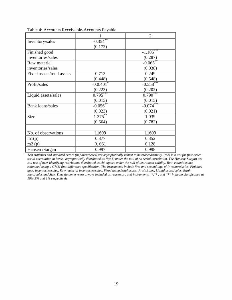
Turning to results for net trade credit (accounts receivable-accounts payable) the coefficient of

total inventories is negative and significant at 5 percent. Once the inventories are bifurcated

both finished goods and raw material inventories have a negative and significant coefficient.

What is important is that the finished goods inventories have a much larger coefficient. Thus it

is finished good inventories that are more influential in determining net trade credit given. The

coefficients of profits and bank loans have a negative and significant sign while liquid assets

have a positive and significant sign. Size turns out to be insignificant in both specifications.

4. Conclusions

The empirical evidence presented suggests that in the Indian context strong evidence exists in

support of an inventory management motive for offering trade credit. Firms attempt to increase

sales and lower finished goods inventories by offering trade credit both on a gross and net

basis. When inventories of finished goods and semi finished goods and raw materials rise firms

tend to postpone payments to their supplier and this shows up on their books of accounts as

higher accounts payable. This is likely to help firms tide over negative shocks to sales. Thus

trade credit in general can be seen to arise as a financial response to variable demand for their

finished goods. Highly profitable firms are found to both give (on both net and gross basis) and

receive less trade credit. There could be many underlying results for this finding. Firstly more

profitable firms may not face a major problem with respect to variability of demand for their

product. The need to offer trade credit for inventory management is thus smaller. Moreover the

need to accept trade credit for such firms would also be lower, as inventories would rarely he

high. Secondly, as argued by Burkart and Ellingsen (2004), profitable but finance constrained

firms would prefer not to offer trade credit. The fact that the coefficients of profitability are

negative, price discrimination does not seem to be a motive for the existence of trade credit in

India.

Firm’s holdings of liquid assets have a positive influence on accounts receivable and accounts

payable and net trade credit. Firms with greater access to bank credit offer less trade credit to

their customers. Firms with more access to bank funds do not pass them on to their buyers as

accounts receivable. On the other hand, firms with higher bank loans receive more trade credit.

The empirical results on the determinants of trade credit in India are very different from those

for advanced countries.

14

References:

Athey M.J. and P.S. Laumas(1994) “Internal funds and Corporate Investments in India”

Journal of Development Economics, 45, pp 287-303.

Biais B.and C.Gollier (1997) “Trade Credit and Credit Rationing” Review of Financial Studies,

10(4), pp903-937

Bougheas S., Mateut S. and P.Mizen (2009) “Corporate Trade Credit and Inventories: New

Evidence of a Trade –off from Accounts Payable and Receivable” Journal of Banking and

Finance, 33, pp 300-307.

Brennan M.J., V. Maksimovic and J. Zechner (1988) “Vendor Financing” Journal of Finance,

43(5), 1127-1141.

Burkart M. and T. Ellingson (2004) “In-Kind Finance : A Theory of Trade Credit” American

Economic Review, 94(3), 569-590.

Cunat V. (2007) “Trade Credit: Suppliers as Debt Collectors and Insurance Providers” The

Review of Financial Studies, 20(2), pp 491-527

Cunningham R.(2004) “Trade Credit and Credit Rationing in Canadian Firms” Bank of Canada

Working paper 2004-49.

Deloof M. and M.Jegers (1999) “Trade Credit, Corporate Groups and the Financing of Belgian

Firms” Journal of Business Finance and Accounting, 26(7), pp 945-966.

Emery G. (1987) “An optimal financial response to variable demand”, Journal of Finance and

Quantitative Analysis, 22 (2), pp.209-25.

Ganesh_Kumar A. Sen K. and R.R. Vaidya (2001) “Outward Orientation, investment and

finance constraints: A study of Indian firms” Journal of Development Studies, 37(4), pp 133-

149.

Guariglia A. and S. Mateut (2006) “Credit Channel, Trade Credit Channel and Inventory

Investment :Evidence from a Panel of U.K. Firms” Journal of Banking and Finance, 30, pp

2835-2856.

Jain N. (2001) “Monitoring Costs and Trade Credit” Quarterly Review of Economics and

Finance, 41, pp 89-110.

Kohler M., Britton E. and T. Yates (2000) “Trade Credit and the Monetary Transmission

Mechanism” Bank of England, Working Paper.

Lensink R, Remco van der Molen and S. Gangopadhay (2003) “Business Groups, Financing

Constraints and Investment: The Case of India” Journal of Development Studies, 40(2), pp 93-

119.

15

Lee Y.W. and J.D. Stowe (1993) “Product Risk, Asymmetric Information and Trade Credit”

The Journal of Financial and Quantitative Analysis” 28(2), pp 285-300.

Mateut S, Bougheas S. and P. Mizen (2006) “Trade credit, bank lending and monetary policy

transmission” European Economic Review, 50( 3), pp 603-629.

Metzler A.H.(1960) “Mercantile Credit, Monetary Policy and Size of Firms” The Review of

Economics and Statistics, 42(4),pp 429-437.

Miwa Y. and J.M. Ramseyer (2005) “Trade Credit, Bank Loans and Monitoring: Evidence

from Japan” CARF Working Paper F-054.

Nilsen J. (2002) “Trade Credit and the bank lending Channel” Journal of Money Credit and

Banking, 34, pp 226-253.

Ng C., Smith J. and R. Smith (1999) “Evidence on the Determinants of Credit Terms in Inter

firm Trade” Journal of Finance, 54, pp 1109-1129.

Petersen M.A. and R.G. Rajan (1997) “Trade Credit: Theories and Evidence” The Review of

Financial Studies” 10(3), pp 661-691.

Rajan R.G. and L. Zingales (1995) “What do we know about capital structure? Some evidence

from international data”, Journal of Finance, 50, pp 1421-1460.

Report of the Working Group on Discounting of Bills by Banks (2000), Reserve Bank of India,

Mumbai.

Roodman D. (2005) “Xtabond2:Stat module to extend xtabond dynamic panel data estimator”

Working paper, Center for Global Development, Washington.

Schwartz R. (1974) “An Economic Model of Trade Credit” Journal of Financial and

Quantitative Analysis, 9, pp 643-657

Van Horne J. (1995) Financial Management and Policy, Prentice Hall.

16

Table1: Summary Statistics (mean, standard deviation and median)

Bottom 25% Middle 50% Top 25% Whole sample

Accounts Receivable/sales Mean 0.357 0.213 0.175 0.240

Std. Dev 3.620 1.496 0.172 2.101

Median 0.184 0.165 0.144 0.162

Accounts Payable/sales Mean 0.210 0.157 0.157 0.170

Std. Dev 0.496 0.299 0.306 0.361

Median 0.120 0.116 0.125 0.120

(Accounts Receivable-Accounts

payable)/sales Mean

0.147 0.057 0.018 0.070

Std. Dev 3.496 1.456 0.302 2.036

Median 0.050 0.042 0.018 0.038

Inventories/sales Mean 0.193 0.127 0.113 0.140

Std. Dev 0.846 0.262 0.218 0.476

Median 0.079 0.079 0.079 0.079

Finished good inventories/sales Mean 0.119 0.086 0.081 0.093

Std. Dev 0.438 0.230 0.195 0.290

Median 0.041 0.045 0.052 0.046

Raw material inventories/sales Mean 0.245 0.127 0.107 0.152

Std. Dev 2.614 0.317 0.176 1.331

Median 0.086 0.090 0.079 0.086

Fixed assets/Total assets Mean 0.637 0.636 0.670 0.645

Std. Dev 0.348 0.279 0.264 0.295

Median 0.601 0.631 0.670 0.634

Profit/sales Mean 0.035 0.101 0.159 0.099

Std. Dev 4.508 1.544 0.158 2.508

Median 0.087 0.120 0.149 0.121

Liquid Assets/sales Mean 0.363 0.088 0.100 0.160

Std. Dev 6.708 0.697 0.342 3.399

Median 0.028 0.027 0.043 0.031

Bank loans/sales Mean 0.351 0.205 0.154 0.229

Std. Dev 3.722 2.335 0.319 2.495

Median 0.105 0.120 0.105 0.113

Size Mean 2.023 3.822 5.916 3.894

Std. Dev 0.662 0.670 0.931 1.566

Median 2.111 3.805 5.716 3.803

Note: Firms are separated into size categories by using a dummy variable which takes the value of 1 in a given year if the firms

total assets are in the top 25, middle 50 and bottom 25 percentile of the distribution of total assets of all the firms in that year.

17

Table 2: Accounts Receivable

1 2

Inventories/sales

-0.715**

(0.312)

Finished good

inventories/sales

-0.915***

(0.306)

Raw material

inventories/sales

0.032

(0.041)

Fixed assets/total assets 0.622*

(0.376)

0.209

(0.481)

Profit/sales -0.455**

(0.195)

-0.557***

(0.202)

Liquid assets/sales 0.833***

(0.013)

0.823***

(0.016)

Bank loans/sales -0.034

(0.022)

-0.049**

(0.023)

Size 1.427***

(0.530)

1.013

(0.663)

No. of observations 11609 11609

m1(p) 0.00 0.00

m2 (p) 0. 281 0.231

Hansen /Sargan 0.958 0.988 Test statistics and standard errors (in parentheses) are asymptotically robust to heteroscedasticity. (m2) is a test for first order

serial correlation in levels, asymptotically distributed as N(0,1) under the null of no serial correlation. The Hansen/ Sargan test

is a test of over identifying restrictions distributed as chi-square under the null of instrument validity. Both equations are

estimated using a GMM first difference specification. The instruments include first and second lags of Inventory/sales, Finished

good inventories/sales, Raw material inventories/sales, Fixed assets/total assets, Profit/sales, Liquid assets/sales, Bank

loans/sales and Size. Time dummies were always included as regressors and instruments. *,** , and *** indicate significance at

10%,5% and 1% respectively.

18

Table 3: Accounts Payable

1 2

Inventory/sales

0.103***

(0.061)

Finished good

inventories/sales

0.256***

(0.049)

Raw material

inventories/sales

0.104***

(0.010)

Fixed assets/total assets -0.171

(0.131)

-0.073

(0.118)

Profit/sales -0.079**

(0.034)

-0.025

(0.027)

Liquid assets/sales 0.033***

(0.002)

0.034***

(0.001)

Bank loans/sales 0.024**

(0.011)

0.027**

(0.011)

Size -0.070

(0.172)

-0.218

(0.158)

No. of observations 11609 11609

m1(p) 0.084 0.269

m2 (p) 0.333 0.374

Hansen /Sargan 0.410 0.870 Test statistics and standard errors (in parentheses) are asymptotically robust to heteroscedasticity. (m2) is a test for first order

serial correlation in levels, asymptotically distributed as N(0,1) under the null of no serial correlation. The Hansen/ Sargan test

is a test of over identifying restrictions distributed as chi-square under the null of instrument validity. Both equations are

estimated using a GMM first difference specification. The instruments include first and second lags of Inventory/sales, Finished

good inventories/sales, Raw material inventories/sales, Fixed assets/total assets, Profit/sales, Liquid assets/sales, Bank

loans/sales and Size. Time dummies were always included as regressors and instruments. *,** , and *** indicate significance at

10%,5% and 1% respectively.

19

Table 4: Accounts Receivable-Accounts Payable

1 2

Inventory/sales

-0.354**

(0.172)

Finished good

inventories/sales

-1.185***

(0.287)

Raw material

inventories/sales

-0.065**

(0.038)

Fixed assets/total assets 0.713

(0.448)

0.249

(0.548)

Profit/sales -0.0.401*

(0.223)

-0.558***

(0.202)

Liquid assets/sales 0.795***

(0.015)

0.790***

(0.015)

Bank loans/sales -0.056**

(0.023)

-0.074***

(0.021)

Size 1.375**

(0.664)

1.039

(0.782)

No. of observations 11609 11609

m1(p) 0.377 0.352

m2 (p) 0. 661 0.128

Hansen /Sargan 0.997 0.998 Test statistics and standard errors (in parentheses) are asymptotically robust to heteroscedasticity. (m2) is a test for first order

serial correlation in levels, asymptotically distributed as N(0,1) under the null of no serial correlation. The Hansen/ Sargan test

is a test of over identifying restrictions distributed as chi-square under the null of instrument validity. Both equations are

estimated using a GMM first difference specification. The instruments include first and second lags of Inventory/sales, Finished

good inventories/sales, Raw material inventories/sales, Fixed assets/total assets, Profit/sales, Liquid assets/sales, Bank

loans/sales and Size. Time dummies were always included as regressors and instruments. *,** , and *** indicate significance at

10%,5% and 1% respectively.