the design of modern steel bridges -...

The Design ofModern Steel Bridges

Second Edition

Sukhen ChatterjeeBE, MSc, DIC, PhD, FICE, MIStructE


Second Edition

Sukhen ChatterjeeBE, MSc, DIC, PhD, FICE, MIStructE

# Sukhen Chatterjee, 1991, 2003

Blackwell Science Ltd, a BlackwellPublishing CompanyEditorial Offices:Osney Mead, Oxford OX2 0EL, UKTel: +44 (0)1865 206206

Blackwell Publishing, Inc., 350 MainStreet, Malden, MA 02148-5018, USATel: +1 781 388 8250

Iowa State Press, a Blackwell PublishingCompany, 2121 State Avenue, Ames, Iowa50014-8300, USATel: +1 515 292 0140

Blackwell Publishing Asia Pty Ltd,550 Swanston Street, Carlton South,Victoria 3053, AustraliaTel: +61 (0)3 9347 0300

Blackwell Wissenschafts Verlag,Kurfurstendamm 57, 10707 Berlin,GermanyTel: +49 (0)30 32 79 060

The right of the Author to be identified asthe Author of this Work has been assertedin accordance with the Copyright, Designsand Patents Act 1988.

All rights reserved. No part of thispublication may be reproduced, stored in aretrieval system, or transmitted, in any formor by any means, electronic, mechanical,photocopying, recording or otherwise,except as permitted by the UK Copyright,Designs and Patents Act 1988, without theprior permission of the publisher.

First edition published 1991This edition first published 2003 byBlackwell Science Ltd

Library of CongressCataloging-in-Publication Datais available

ISBN 0-632-05511-1

A catalogue record for this title is availablefrom the British Library

Set in Times and produced by GrayPublishing, Tunbridge Wells, KentPrinted and bound in Great Britain byMPG Books Ltd, Bodmin, Cornwall

For further information onBlackwell Science, visit our website:www.blackwell-science.co.uk

Contents

Preface viiAcknowledgements ix

1 Types and History of Steel Bridges 11.1 Bridge types 11.2 History of bridges 2

2 Types and Properties of Steel 372.1 Introduction 372.2 Properties 382.3 Yield stress 392.4 Ductility 412.5 Notch ductility 412.6 Weldability 442.7 Weather resistance 452.8 Commercially available steels 452.9 Recent developments 48References 48

3 Loads on Bridges 513.1 Dead loads 513.2 Live loads 513.3 Design live loads in different countries 533.4 Recent developments in bridge loading 583.5 Longitudinal forces on bridges 633.6 Wind loading 643.7 Thermal forces 683.8 Other loads on bridges 713.9 Load combinations 71References 73

v

4 Aims of Design 754.1 Limit state principle 754.2 Permissible stress method 764.3 Limit state codes 774.4 The derivation of partial safety factors 794.5 Partial safety factors in BS 5400 86References 90

5 Rolled Beam and Plate Girder Design 915.1 General features 915.2 Analysis for forces and moments 945.3 Lateral buckling of beams 965.4 Local buckling of plate elements 1095.5 Design of stiffeners in plate girders 1355.6 Restraint at supports 1485.7 In-plane restraint at flanges 1495.8 Design example of a stiffened girder web 153References 158

6 Stiffened Compression Flanges of Box and Plate Girders 1596.1 General features 1596.2 Buckling of flange plate 1606.3 Overall buckling of strut 1626.4 Allowance for shear and transverse stress in flange plate 1646.5 Orthotropic buckling of stiffened flange 1656.6 Continuity of longitudinal stiffeners over transverse

members 1696.7 Local transverse loading on stiffened compression flange 1736.8 Effect of variation in the bending moment of a girder 1746.9 Transverse stiffeners in stiffened compression flanges 174

6.10 Stiffened compression flange without transverse stiffeners 1776.11 A design example of stiffened compression flange 178References 182

7 Cable-stayed Bridges 1837.1 History 1837.2 Cable-stay systems 1877.3 Cable types 1887.4 Cable properties 1957.5 Design and construction of a cable-stayed bridge 199

Reference 201

Index 203

vi Contents

Preface

Bridges are great symbols of mankind’s conquest of space. The sight of thecrimson tracery of the Golden Gate Bridge against a setting sun in the Pacific

Ocean, or the arch of the Garabit Viaduct soaring triumphantly above the deepgorge, fills one’s heart with wonder and admiration for the art of their builders.

They are the enduring expressions of mankind’s determination to remove allbarriers in its pursuit of a better and freer world. Their design and buildingschemes are conceived in dream-like visions. But vision and determination are

not enough. All the physical forces of nature and gravity must be understoodwith mathematical precision and such forces have to be resisted by mani-

pulating the right materials in the right pattern. This requires both the inspira-tion of an artist and the skill of an artisan.

Scientific knowledge about materials and structural behaviour has expandedtremendously, and computing techniques are now widely available to mani-

pulate complex theories in innumerable ways very quickly. But it is still notpossible to accurately cater for all the known and unknown intricacies. Eventhe most advanced theories and techniques have their approximations and

exceptions. The wiser the scientist, the more he knows of his limitations.Hence scientific knowledge has to be tempered with a judgement as to how far

to rely on mathematical answers and then what provision to make for theunknown realities. Great bridge-builders like Stephenson and Roebling pro-

vided practical solutions to some very complex structural problems, for whichcorrect mathematical solutions were derived many years later; in fact the clue

to the latter was provided by the former.Great intuition and judgement spring from genius, but they can be helped

along the way by an understanding of the mathematical theories. The object ofthis book is to explain firstly the nature of the problems associated with thebuilding of bridges with steel as the basic material, and then the theories that

are available to tackle them. The reader is assumed to have the basic degree-level knowledge of civil engineering, i.e. he or she may be a final-year

undergraduate doing a project with bridges, or a qualified engineer enteringinto the field of designing and building steel bridges.

The book sets out with a technological history of the gradual development ofdifferent types of iron and steel bridges. A knowledge of this evolution from

the earliest cast-iron ribbed arch, through the daring suspension and arch

vii

structures, on to the modern elegant plated spans, will contribute to a proper

appreciation of the state-of-the-art today.The basic properties of steel as a building material, and the successive

improvement achieved by the metallurgist at the behest of the bridge-builder,are then described. The natural and the traffic-induced forces and phenomena

that the bridge structure must resist are then identified and quantified withreference to the practices in different countries. This is followed by an explana-

tion of the philosophy behind the process of the structural design of bridges,i.e. the basic functional aims and how the mathematical theories are applied to

achieve them in spite of the unavoidable uncertainties inherent in naturalforces, in idealised theories and in the construction processes. This subject istreated in the context of limit state and statistical probability concepts. Then

follows detailed guidance on the design of plate and box girder bridges, themost common form of construction adopted for steel bridges in modern times.

The buckling behaviour of various components, the effects of geometricalimperfections and large-deflection behaviour, and the phenomenon of post-

buckling reserves are described in great detail. The rationale behind therequirements of various national codes and the research that helped their

evolution are explained, and a few design examples are worked out to illustratetheir intended use.In the second edition of this book, the history of steel bridges has been

updated with brief descriptions of the latest achievements in building long-span steel bridges. A new chapter on cable-stayed steel bridges has been added,

which describes the historical developments of this type of construction, thetypes and properties of different cables and how cable properties can be used in

the design and construction of such bridges.Many of the changes introduced in the latest version of the British Standard

Design Code for Steel Bridges, BS 5400: Part 3: 2000 are explained, forexample in the design clauses for lateral torsional buckling of beams, brittle

fracture/notch ductility requirements and the effect of elastic curvature andcamber of girders on longitudinal flange stiffeners. More refined treatments forthe design of longitudinal and transverse stiffeners on the webs of plate and

box girders and for the intermediate and support restraints against lateraltorsional buckling of plate girders are included.

The latest specification requirements for structural steel in the westernEuropean countries are tabulated. Finally, a simple manual method is given for

evaluating the failure probability of a structure subjected to a number ofuncorrelated loadings and the resistance of which is a product function of

uncorrelated variables like material strength and structural dimensions.

Sukhen Chatterjee

viii Preface

Acknowledgements

The figures in Chapter 1 are reproduced with kind permission of the following:

Flint & Neill Partnership, London – Figures 1.5, 1.10, 1.15, 1.16, 1.17, 1.22,1.32, 1.33 and 1.39.

Steel Construction Institute, Ascot – Figures 1.8, 1.20, 1.25, 1.28, 1.31, 1.35,1.37 and 1.40 (from the collection of late Bernard Godfrey).

Acer, Guildford – Figures 1.13, 1.14, 1.19, 1.24, 1.34 and 1.36.

Rendel, High-Point, London – Figures 1.6, 1.11, 1.12 and 1.29.

Institution of Civil Engineers, London – Figures 1.3, 1.7 and 1.30.

Mr B Oakhill of BCSA, London – Figure 1.26.

Symmonds Group, East Grinstead – Figure 1.38.

Professor J Harding of Surrey University – Figure 1.23.

Steinman, Boynton, Gronquist & London of New York – Figure 1.18.

The front cover design is from a photograph of the Second Severn Crossingbetween England and Wales, courtesy of Faber-Maunsell Group.

ix

Chapter 1

Types and History of Steel Bridges

1.1 Bridge types

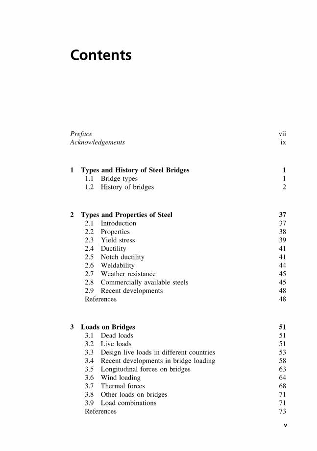
There are five basic types of steel bridges:

(1) Girder bridges – flexure or bending between vertical supports is the main

structural action in this type. They may be further sub-divided into simplespans, continuous spans and suspended-and-cantilevered spans as illus-

trated in Fig. 1.1.(2) Rigid frame bridges – in this type the longitudinal girders are made

structurally continuous with the vertical or inclined supporting members

Arch bridges Girder bridges

Continuous spans

Discontinuous spans

Rigid frame bridges

Suspension bridge

Suspended-and-cantilever spans

Cable-stayed bridges

Figure 1.1 Different types of bridges.

1

by means of moment-carrying joints; flexure with some axial force is the

main structural action in this type.(3) Arches – in which the loads are transferred to the foundations by arches

as the main structural element; axial compression in the arch rib is the mainstructural action, combined with some bending. The horizontal thrust at

the ends is resisted either by the foundations or by a tie running longitudin-ally for the full span length; the latter type is called a tied or a bow-

string arch.(4) Cable-stayed bridges – in which the main longitudinal girders are

supported by a few or many ties in the vertical or near-vertical plane,which are hung from one or more tall towers and are usually anchoredat the bottom to the girders.

(5) Suspension bridges – in which the bridge deck is suspended from cablesstretched over the gap to be bridged, anchored to the ground at two ends

and passing over tall towers erected at or near the two edges of the gap.

The first three types and the deck structure of the last two types of bridgesmay be either solid-web girders or truss (or lattice) girders.

1.2 History of bridges

1.2.1 Iron bridges

Iron was used in Europe for building cannons and machinery in the sixteenth

century, but it was not until the late eighteenth century, in the wake of the firstindustrial revolution, that iron was first used for structures. The world’s first

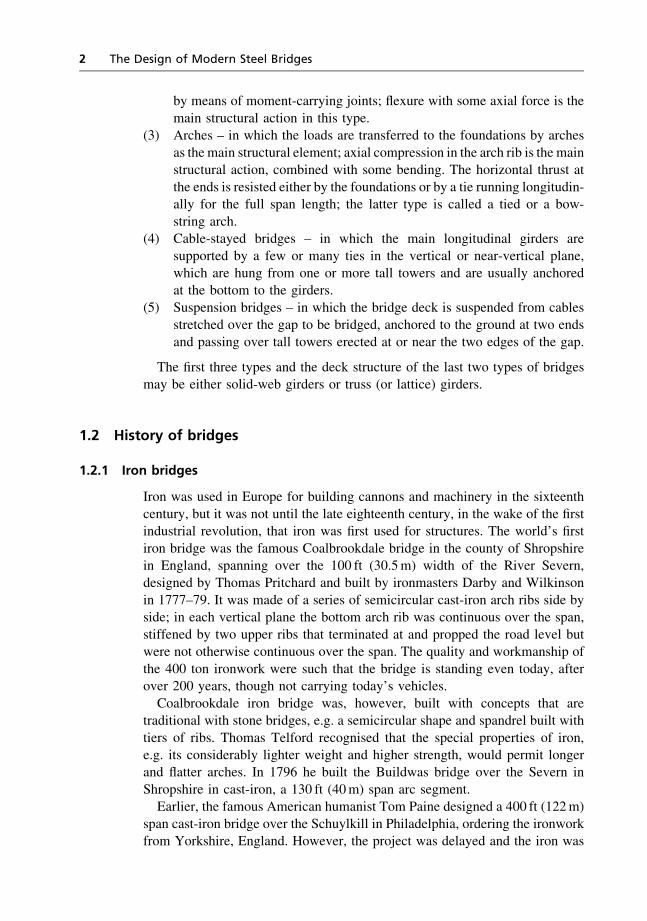
iron bridge was the famous Coalbrookdale bridge in the county of Shropshirein England, spanning over the 100 ft (30.5m) width of the River Severn,designed by Thomas Pritchard and built by ironmasters Darby and Wilkinson

in 1777–79. It was made of a series of semicircular cast-iron arch ribs side byside; in each vertical plane the bottom arch rib was continuous over the span,

stiffened by two upper ribs that terminated at and propped the road level butwere not otherwise continuous over the span. The quality and workmanship of

the 400 ton ironwork were such that the bridge is standing even today, afterover 200 years, though not carrying today’s vehicles.

Coalbrookdale iron bridge was, however, built with concepts that aretraditional with stone bridges, e.g. a semicircular shape and spandrel built with

tiers of ribs. Thomas Telford recognised that the special properties of iron,e.g. its considerably lighter weight and higher strength, would permit longerand flatter arches. In 1796 he built the Buildwas bridge over the Severn in

Shropshire in cast-iron, a 130 ft (40m) span arc segment.Earlier, the famous American humanist Tom Paine designed a 400 ft (122m)

span cast-iron bridge over the Schuylkill in Philadelphia, ordering the ironworkfrom Yorkshire, England. However, the project was delayed and the iron was

2 The Design of Modern Steel Bridges

used to build a 236 ft (72m) span bridge over the Wear in Sunderlandsimultaneously with Buildwas. These bridges led the way to many more iron

bridges in the first two decades of the nineteenth century in England andFrance, the most notable being the Vauxhall and Southwark bridges over the

Thames in London (each using over 6000 tons of iron) and Pont du Louvre andPont d’Austerlitz over the Seine in Paris (the latter has since been replaced). In

the early days cast-iron was slotted and dovetailed like timber constructionbefore bolting was discovered.In 1814 Thomas Telford proposed a suspension bridge with cables made of

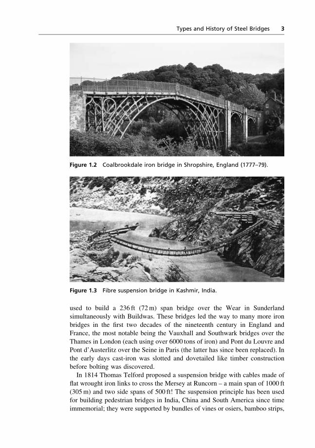
flat wrought iron links to cross the Mersey at Runcorn – a main span of 1000 ft(305m) and two side spans of 500 ft! The suspension principle has been used

for building pedestrian bridges in India, China and South America since timeimmemorial; they were supported by bundles of vines or osiers, bamboo strips,

Figure 1.2 Coalbrookdale iron bridge in Shropshire, England (1777–79).

Figure 1.3 Fibre suspension bridge in Kashmir, India.

Types and History of Steel Bridges 3

plaited ropes, etc., and sometimes even had plank floors and hand rails.Telford, collaborating with Samuel Brown, made experiments with wroughtiron and decided that cables made of wrought iron eyebar chains could be used

with a working stress of 5 tons per square inch (77N/mm2), compared withonly 1.25 tons/in2 tensile working stress of cast-iron. The Mersey bridge did

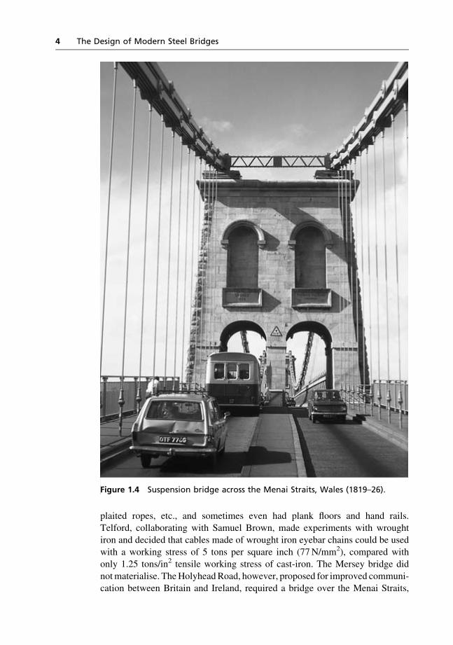
notmaterialise. TheHolyheadRoad, however, proposed for improved communi-cation between Britain and Ireland, required a bridge over the Menai Straits,

Figure 1.4 Suspension bridge across the Menai Straits, Wales (1819–26).


and Telford proposed in 1817 a suspension bridge of 580 ft (177m) main span.Work on site started in 1819, and in 1826 the world’s first iron suspension

bridge for vehicles was completed. This was also the world’s first bridge oversea water. The bridge had 100 ft (30.5m) clearance over the high water of the

Irish Sea and took 2000 tons of wrought iron (compared with 6000 tons of ironfor the Vauxhall arch bridge). It had no stiffening girder and no wind bracing;

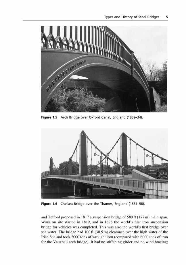
Figure 1.5 Arch Bridge over Oxford Canal, England (1832–34).

Figure 1.6 Chelsea Bridge over the Thames, England (1851–58).


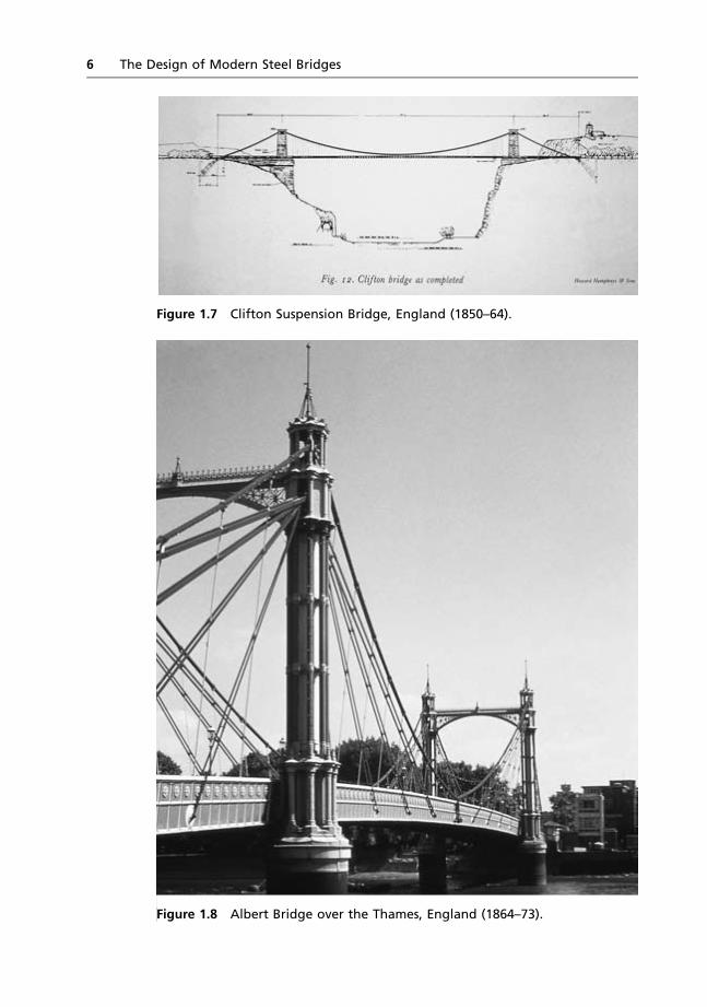
Figure 1.7 Clifton Suspension Bridge, England (1850–64).

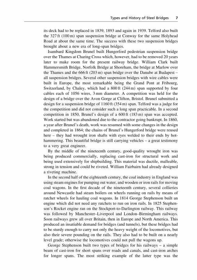
Figure 1.8 Albert Bridge over the Thames, England (1864–73).


its deck had to be replaced in 1839, 1893 and again in 1939. Telford also built

the 327 ft (100m) span suspension bridge at Conway for the same HolyheadRoad at about the same time. The success with these two suspension bridges

brought about a new era of long-span bridges.Isambard Kingdom Brunel built Hungerford pedestrian suspension bridge

over the Thames at Charing Cross which, however, had to be removed 20 yearslater to make room for the present railway bridge. William Clark built

Hammersmith Bridge, Norfolk Bridge at Shoreham, the bridge at Marlow overthe Thames and the 666 ft (203m) span bridge over the Danube at Budapest –

all suspension bridges. Several other suspension bridges with wire cables werebuilt in Europe, the most remarkable being the Grand Pont at Fribourg,Switzerland, by Chaley, which had a 800 ft (244m) span supported by four

cables each of 1056 wires, 3mm diameter. A competition was held for thedesign of a bridge over the Avon Gorge at Clifton, Bristol. Brunel submitted a

design for a suspension bridge of 1160 ft (354m) span. Telford was a judge forthe competition and did not consider such a long span practicable. In a second

competition in 1850, Brunel’s design of a 600 ft (183m) span was accepted.Work started but was abandoned due to the contractor going bankrupt. In 1860,

a year after Brunel’s death, work was resumed with some changes in the designand completed in 1864; the chains of Brunel’s Hungerford bridge were reusedhere – they had wrought iron shafts with eyes welded to their ends by hot-

hammering. This beautiful bridge is still carrying vehicles – a great testimonyto a very great engineer.

By the middle of the nineteenth century, good-quality wrought iron wasbeing produced commercially, replacing cast-iron for structural work and

being used extensively for shipbuilding. This material was ductile, malleable,strong in tension and could be riveted. William Fairbairn had already designed

a riveting machine.In the second half of the eighteenth century, the coal industry in England was

using steam engines for pumping out water, and wooden or iron rails for movingcoal wagons. In the first decade of the nineteenth century, several collieriesaround Newcastle had steam boilers on wheels running on rails by means of

ratchet wheels for hauling coal wagons. In 1814 George Stephenson built anengine which did not need any ratchets to run on iron rails. In 1825 Stephen-

son’s Rocket engine ran on the Stockport-to-Darlington railway. This railwaywas followed by Manchester–Liverpool and London–Birmingham railways.

Soon railways grew all over Britain, then in Europe and North America. Thisproduced an insatiable demand for bridges (and tunnels), but these bridges had

to be sturdy enough to carry not only the heavy weight of the locomotives, butalso their severe pounding on the rails. They also had to be built on a nearlylevel grade; otherwise the locomotives could not pull the wagons up.

George Stephenson built two types of bridges for his railways – a simplebeam of cast-iron for short spans over roads and canals, and cast-iron arches

for longer spans. The most striking example of the latter type was the


Newcastle High Level Bridge; his son Robert played a significant part in its

design and construction. The bridge consisted of six bow-string arches, eachwith a horizontal tie between the springing points to resist the end thrust, with

the railway on the top and the road suspended underneath by wrought iron rods120 ft (37m) above water. It was completed in August 1849 and a few days

after the opening Queen Victoria stopped her train on it to admire the view.Robert Stephenson was already considering how to cross the Menai Straits

and the Conway river for his Chester–Holyhead Railway. Suspension bridgesbuilt up to then to carry horse-drawn carriages exhibited a lack of rigidity and

a weakness in windy conditions, and hence could not possibly withstand theheavy and rhythmic pounding of locomotives. Several such bridges carryingroads had either fallen down or suffered great damage; for example, the one at

Broughton had collapsed under a column of marching soldiers and the chain-pier bridge at Brighton had been blown down by a storm. This list also

included bridges at Tweed, Nassau in Germany, Roche Bernard in France andseveral in America.

The first suspension bridge to carry a railway was built by Samuel Brown in1830 over the Tees; it sagged when a train came over it, and the engine could

not climb up the steep gradient that the deflection of the structure formed aheadof it. Robert Stephenson decided that Telford’s road bridge solution of asuspension bridge would not be appropriate to carry a railway over the Menai

Straits, nor could a cast-iron arch be built here, as the Admiralty would permitneither the reduction in headroom near the springing points of the arch

construction nor the temporary navigational blockage that the timber centringwould cause. Stephenson had already decided that a rocky island in the Menai

channel called the Britannia Rock would support an intermediate pier.Stephenson hit upon the idea of two massive wrought iron tubes through

which the trains could run. At his request William Fairbairn conducted tests oncircular, rectangular and elliptical shapes, and also on wrought iron stiffened

and cellular panels for their compressive strength. The Conway crossing wasready first, and in 1848 two huge tubes 400 ft (122m) long were floated out onpontoons, lifted up and placed in their correct positions during a falling tide. A

year later, in 1849, the four tubes of the Menai crossing, two 460 ft (140m) andtwo 230 ft (70m) spans, were similarly erected. As box girder bridges, they

were highly ingenious and unique for many decades; they were also the giantforerunners of thousands of plate girder bridges that became the most popular

type of bridge construction all over the world. The Britannia Bridge at Menaiwas severely damaged by a fire in May 1970 and had to be rebuilt in the shape

of a spandrel braced arch as originally proposed by Rennie and Telford.A roadway was also added on an upper level.In the United States, railroad construction started in the early 1830s. The

early railway bridges were mostly patented truss types (‘Howe’, ‘Pratt’,‘Warren’, etc.) with wooden compression members and wrought-iron tension

members. These were followed by a composite truss system of cast-iron


compression members and wrought-iron tension members. In 1842 Charles

Ellet built a suspension bridge over Schuylkill river at Fairmont, Pennsylvania,to replace Lewis Wernwag’s 340 ft (104m) span Colossus Bridge destroyed by

fire. The latter was a timber bridge formed in the shape of a gently curved archreinforced by trusses the diagonals of which were iron rods – the first use of iron

in a long-span bridge in America. Ellet’s suspended span was supported by tenwire cables. In 1848 Ellet started to build the first ever bridge across the 800 ft

(244m) wide chasm below the Niagara Falls to carry a railway. To carry thefirst wire, he offered a prize of five dollars to fly a kite across. After the first wire

cable was stretched in this way, the showman that he was, he hauled himselfacross the gorge in a wire basket at a height of 250 ft (76m) above the swirlingwater! He then built a 7.5 ft (2.3m) wide service bridge without railings,

rode across on a horse and started collecting fares. Then he fell out withthe promoters and withdrew, leading to the appointment of John Roebling, a

Prussian-born engineer, to erect a new bridge. In 1841 Roebling had alreadypatented his idea of forming cables from parallel wires bound into a compact

bunch by binding wire.In 1848 John Ellet had built another suspension bridge of 308m (1010 ft)

span over the Ohio river at Wheeling, West Virginia. In January 1854 itcollapsed in a storm, due to aerodynamic vibration. Roebling realised that ‘thedestruction’ of the Wheeling bridge was clearly ‘owing to a want of stability,

and not to a want of strength’ – his own words. He also studied the collapse ofa suspension bridge in 1850 in Angers, France, under a marching regiment, and

another in Licking, Kentucky, in 1854 under a drove of trotting cattle. HisGrand Trunk bridge at Niagara had a 250m (820 ft) span and had two decks,

the upper one to carry a railway and the lower one a road; stiffening trusses18 ft (5.5m) deep of timber construction were provided between the two

decks – the first stiffening girder used for a suspension bridge. The deck wassupported by four main cables 10 inch (254mm) in diameter consisting of

parallel wrought iron wires, uniformly tensioned and compacted into a bunchwith binding wire.This was the birth of the modern suspension bridge, which must be ranked as

one of history’s greatest inventions. The deck was also supported from thetower directly by 64 diagonal stays, and more stays were later added below the

deck and anchored to the gorge sides. The bridge was completed in 1855.Roebling proved, contrary to Stephenson’s prediction, that suspension bridges

could carry railways and were more economical than the tubular girderconstruction used by the latter at Menai. In reality, however, not many railway

suspension bridges were later built, but Roebling’s Niagara bridge was theforebear of a great number of suspension bridges carrying roads. Its woodendeck was replaced by iron and the masonry towers by steel in 1881 and 1885,

respectively, and finally the whole bridge was replaced in 1897. Two otherbridges were built across the Niagara gorge. Serrell’s road bridge of 1043 ft

(318m) span was built in 1851, stiffened by Roebling by stays in 1855 and


destroyed by a storm in 1864 when the stays were left loose. At the site of the

present Rainbow Bridge, Keefer built a bridge of 1268 ft (387m) span in 1869,which was destroyed by a storm in 1889. John Roebling and his sonWashington

went on to build several more suspension bridges, the most notable being theones at Pittsburgh and Cincinnati, and the Great Brooklyn Bridge in New York.

1.2.2 Steel bridges

In the second half of the nineteenth century steel was developed and started

replacing cast-iron as a structural material. The technique of using compressedair to sink caissons for foundations below water was also developed. In 1855–

59 Brunel built the Chepstow Bridge over the River Wye and the SaltashBridge over the Tamar to carry railways. These were a combination of arch and

suspension structures. A large wrought-iron tube formed the upper chordshaped like an arch; the lower chord was a pair of suspension chains in caten-

ary profile. The tube and the chains were braced together by diagonal ties andvertical struts. The first glimpse of lattice girder bridges can be seen in these

designs. To carry railways over the Rhine in Germany, several bridges werebuilt in the second half of the century, the most remarkable among them being:

(1) Two bridges in Koln built in 1859, each with four spans of 338 ft (103m)with multiple criss-cross lattice main girders 27.9 ft (8.5m) deep.

(2) A bridge at Mainz built in 1882 with four spans of 344 ft (105m), witha combined structural system of an arched top chord, a catenary bottom

chord and a lattice in-filling between them, as in Brunel’s Wye andSaltash bridges.

In America, the end of the Civil War and the spread of railway constructionresulted in growing demands for building bridges. To connect the Illinois and

the Union Pacific railways a bridge was needed over the 1500 ft (457m) widemighty Mississippi river at St Louis, for which James Eads was commissioned

in 1867. The sandy river bed was subject to considerable shift and scour, androck lay at varying depths between 50 and 150 ft (15–45m). Swirling water

rose 40 ft (12m) in summer, and in winter 20 ft (6m) thick chunks of icehurtled down. Eads proposed to sink caissons down to rock level by com-

pressed air – a technique already being used in Europe (by Brunel in Saltash,for example), but often at the cost of illness and fatality of the workmen. Eads

also decided that a suspension bridge would not be stiff enough to carryrailway loading; he proposed one 520 ft (159m) and two 502 ft (153m) spansof lattice arch construction with steel – the first use of the recently discovered

material in a bridge. Bessemer had already converted iron to steel by addingcarbon in 1856 and Siemens developed the open hearth process in 1867. But

the problem was to produce the enormous quantity of this new material toa guaranteed and uniform quality rightly demanded by Eads, for example


a minimum ‘elastic limit’. Money was raised in America and Europe, which

Eads visited to acquaint himself with the latest bridge-building techniques. Hedesigned chords of 18 inch (450mm) diameter tubes made with 1

4 inch (6mm)

thick steel plates. Each length of tube had wrought-iron threaded end piecesshrunk-fit and they were screwed together by sleeve couplings. The two tubes

were spaced 12 ft (3.7m) apart vertically and braced together with diagonalmembers. The arch ribs were erected by cantilevering, with a series of

temporary tie-back cables supported from temporary towers built over thepiers – the first cantilever erection of a bridge superstructure. This method had

to allow for the effects of temperature, the extension of the temporary cablesand the compression of the arch rib, and one of the fund-raising conditions wasto have to close the first arch by 19 September 1873. This closure was just

achieved, but the span had to be packed with ice at night in order to insert theclosing piece in the final gap. The bridge carried two rail tracks on the bottom

deck and a roadway on top, and is still in use. This bridge was the precursor ofa glittering series of engineering achievements in America, which made it the

most prosperous country in the world.In the 1850s and 1860s in America many truss bridges were built for the

railway lines, but many of them fell down. Buckling of compression memberswas the frequent cause of these failures. The worst disaster was the collapse ofsuch a bridge 157 ft (48m) long in Ashtabula, Ohio, on 29 December 1876,

when during a snow storm a train fell down from it and 80 passengers died.Three years later, on 28 December 1879, 18 months after its completion, the

Tay bridge in Scotland collapsed in a storm with 75 lives lost. Designed byThomas Bouch, this 2mile long bridge had 13 navigation spans of 245 ft

(75m), made of wrought-iron trusses high above the water. In the subsequentenquiry it was established that the design did not allow for adequate horizontal

wind loading. This was the first known example of a bridge failure due to thestatic horizontal pressure of wind drag, as opposed to the many failures of the

early suspension bridges due to aerodynamic oscillations. The Tay Bridge wasrebuilt, and all subsequent bridges were designed for a Board of Tradespecified wind pressure of 56 lb per square foot (2.7 kN/m2). In America, com-

petitive supply of patented bridge types was subjected to a stricter regime ofgovernment regulations and independent supervision. Waddell led the move-

ment for independent bridge design and supervision by consulting engineers;he himself was responsible for building hundreds of major bridges.

In 1867 John Roebling and his son Washington started to build Brooklynbridge connecting Manhattan with Brooklyn in New York across East river. Its

span of 1596 ft (487m) nearly doubled the previous longest span built and ithad to carry two railway lines, two tram-lines, a roadway and a footway. JohnRoebling died in 1869 due to an accident on the site, Washington completing

the construction in 1883. Caissons were sunk by compressed air, amidst prob-lems of ‘caisson disease’ (which crippled Washington himself), ‘blowing’ and

fire. John Roebling’s design pioneered the use of steel cables to support the deck


structure of a bridge. Galvanised cast steel wires of 16 000 lb/in2 (110N/mm2)

tensile strength were specified for the main cables; they were spun wire by wireby the then radical spinning method. To provide stability against wind forcesand to supplement the capacity of the main cables, the suspended deck was

held by diagonal cable stays radiating from the tower top. The graceful yetrobust structure of Brooklyn Bridge was a landmark of human achievement,

vision and determination.The second half of the nineteenth century saw great advances in materials,

machines and structural theories. Use of steel, banned in bridge construction inBritain by the Board of Trade until 1877, became common. Air compressors

and hydraulic machines were developed for aiding construction. James ClerkMaxwell, Rankine and other engineering professors developed theories foranalysis of suspension cables, lattice girders, bending moments and shear

forces in beams, deflection calculations and buckling of struts. These develop-ments and the unsuitability of suspension bridges for carrying railways,

Figure 1.9 Brooklyn Bridge, New York (1867–83).

Figure 1.10 Forth Railway Bridge, Scotland (1881–90).


heralded the era of great trussed cantilever spans, led by the mighty Forth

railway bridge. Designed in 1881 by John Fowler and Benjamin Baker, andconstruction completed in 1890 by Messrs Tancred, Arrol & Co, this bridge

had two massive spans of 1710 ft (521m), each consisting of two 680 ft (207m)cantilevers and a 350 ft (107m) suspended section. The depth of the truss at the

piers was 350 ft (107m). A German engineer called Gerber first developed thecantilever and suspended technique of bridge construction and quite a few such

bridges were also built in America; it had the advantage of requiring no false-work over the gap. Projecting out in both directions, a cantilever structure was

built on each pier and then a short suspended span was hung in between the tipsof the two cantilevers. In the Forth Bridge, Baker built a third main pier on anisland in the midstream, the bridge thus consisting of a triple cantilever with

two suspended spans. The bridge carried two railway tracks 150 ft (46m) abovewater. The specification for the steel required a minimum ultimate strength of

30 ton/in2 (463N/mm2) for tensile members and 34 ton/in2 (525N/mm2) forstruts, and working stresses were a quarter of the ultimate strength. Over 50 000

tons of steel and 6 million rivets were used. This was the first major bridge inEurope built with steel. Unlike cast iron, steel suffers from rusting; paint was

the answer to this problem. The scale of the routine painting operation neededfor the maintenance of Forth Railway Bridge is another facet of its fame.Steel truss bridges started going up all over the world. The Forth Railway

Bridge in Scotland was followed by the Queensboro Bridge over the East Riverin New York which had two main spans of 1182 ft (360m), a central span of

630 ft (192m) and two anchor spans at the two shores – all made continuous intriangulated truss form, without any suspended spans of the Forth sort. This

was followed by the start of construction in 1904 of the Quebec Bridge overthe St Lawrence River in Canada which had a central span of 1800 ft (549m).

The bridge consisted of two giant truss cantilevers on two main piers, witha suspended span in the middle. The two anchor spans were first built on

falsework; then the cantilever arms on the river were erected member bymember by cranes operating on the already erected structure. The twocantilevers having been completed on the two piers in this way, the members

of the suspended spans were also being erected from both sides in this waywhen there were signs of buckling on the web plates of the compression chord

members near the south pier and some rivets were found broken. TheodoreCooper, the respected elderly consulting engineer, who was not present on site,

sent orders to stop erection, but work continued, and on 29 August 1907, thewhole structure collapsed into the river, killing 75 men. In the subsequent

inquiry and investigations it became clear that the lacing system and the splicejoints of the compression members were not able to resist the effects of thebuckling tendency of the compression members. In 1916 a new, slightly wider,

structure was being rebuilt on new foundations; the two cantilevers had beencompleted and the entire 5000 ton suspended span, built on-shore and floated

out, was being lifted up by hydraulic jacks. Then a casting support block at one


corner failed, and the span slid off and fell into the water. The suspended span

was rebuilt and erected successfully a year later.A number of cantilever bridges up to 1644 ft (501m) span have been built in

America; for example:

� Commodore Barry, 1644 ft (501m), Pennsylvania, 1974� Greater New Orleans, 1575 ft (480m), Louisiana, 1958

� East Bay, 1400 ft (427m), San Francisco, 1936.

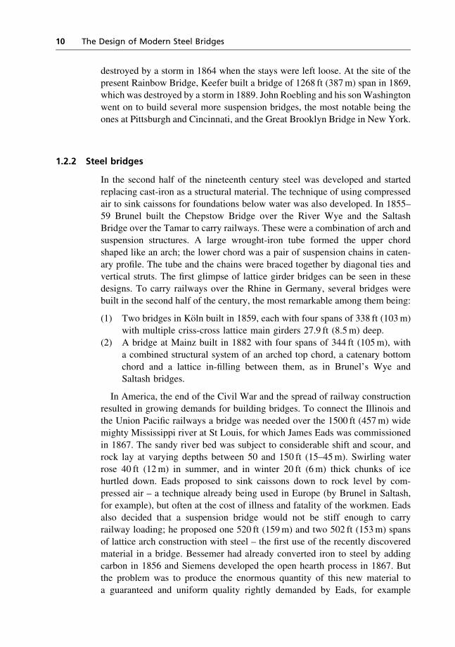
A very remarkable example of this type of construction is the Howrah

Bridge in Kolkata; it had a 1500 ft (457m) central span and 270 ft (82m) highmain towers made in steel and was completed in 1943. The Minato Bridge in

Osaka, Japan, completed in 1974, has a 1673 ft (510m) central span.

Figure 1.11 Howrah Bridge, Kolkata, India.

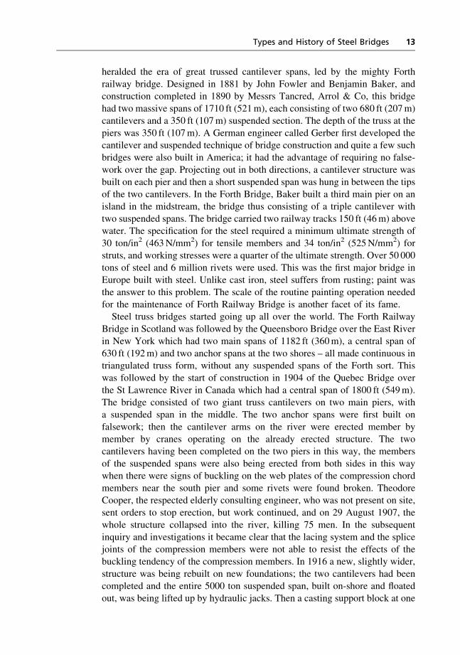
Figure 1.12 Hardinge Bridge, India.


Another form of construction came to bridge the wide waterways in

different parts of the world. The St Louis Bridge of Eads was the forerunner ofthe long-span arch type of bridge. From the later 1860s, several arch spans of

up to 350 ft (107m) were built over the Rhine in Germany. In Oporto, Portugal,two bridges, the Pia Maria and Luiz I, were built, in 1877 and 1885,

respectively, the first by the famous French engineer Gustave Eiffel and thesecond by another Frenchman T. Seyrig. The Luiz I Bridge had a tied arch span

of 560 ft (171m); it carried a road on the top of the arch and its tie carried a railtrack. Eiffel also built, in 1885, the famous Garabit viaduct in the South of

France with an arch span of 540 ft (165m) to carry a railway 400 ft (122m)above a gorge. All these bridges had arch ribs made of wrought iron.In Germany, the Kaiser Wilhelm Bridge at Mungsten, the Dusseldorf–

Oberkassel Bridge and the Bonn–Beuel Bridge over the Rhine were built in

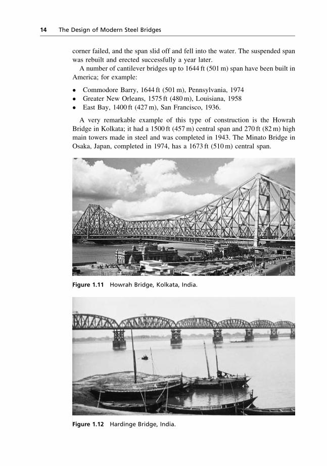
Figure 1.13 Volta Bridge, Africa.


1897–8, of arch spans 170, 181 and 188m (557, 595 and 616 ft), respectively.

The first steel bridge to be built in France was the Viaur Viaduct in southernFrance with a central arch span of 721 ft (220m) carrying a railway. In 1897

the 840 ft (256m) braced-parallel-chord arch span of the Clifton Bridge atNiagara was built, followed by the 950 ft (290m) span box-girder arch rib of

high tensile steel of the Rainbow Bridge. Another historic bridge of this formof construction deserves a mention – the railway bridge over the Zambezi river

near the Victoria Falls in Africa. The 500 ft (152m) span was built in twohalves, cantilevering from each side over the 400 ft (122m) deep gorge, by

British engineers led by Sir Ralph Freeman.The next major arch bridge was the Hell Gate Bridge in New York over the

East River with a span of 977 ft (298m). Designed by Gustav Lindenthal and

completed in 1916, this was a lattice spandrel-braced two-hinged arch of high-carbon steel members and it carried four rail tracks; it is still probably the most

heavily loaded (per unit length) long-span bridge in the world.Next came the Sydney Harbour Bridge. All forms of construction for long-

span bridges, namely suspension, cantilever and arch, were considered fortender competition for its construction in 1923, and the winner was the

spandrel-braced two-hinge steel arch span of 1670 ft (509m) designed by SirRalph Freeman and built by the Dorman Long Company of Middlesborough,England. Completed in 1932, it carried four metro-type rail tracks and a 57 ft

(17m) wide roadway with two footpaths suspended from the arch 172 ft (52m)above water. The bridge took nearly 40 000 tons of steelwork, manufactured in

England and fabricated partly in England and partly in New South Wales.Some of the steel plates and sections broke all previous records in thickness

and size, and tests conducted for the material properties and strength ofmembers provided a wealth of knowledge in steel construction. Erection was

by cantilevering from each side; cranes running on the upper chord of the archlifted up lattice members from the water to be attached to the already erected

cantilever which was temporarily tied back to the banks.

Figure 1.14 Sydney Harbour Bridge, Australia (1923–32).


At about the same time was built, what was until 1977, the longest steel arch

bridge in the world – the 1675 ft (511m) span Bayonne Bridge over the KillVan Kull in New Jersey, designed by Othmar Ammann. The site conditions

permitted the erection of this bridge by temporary trestle, i.e. cantilevering wasnot necessary. The present record for arch span length is held by the bridge

over the New River Gorge at West Virginia, 1700 ft (518m), built in 1977.The great success of the suspension bridge at Brooklyn inspired the building

of Williamsburg and Manhattan Bridges in New York in 1903 and 1909, thelatter designed by Leon Moisseiff using the recently developed ‘deflection

theory for suspension bridges’ by Melan and Steinman, which takes intoaccount second-order deflections of the main cable under live load. After theFirst World War two more bridges of this type were built – the Camden in

Philadelphia in 1926 and the Ambassador in Detroit in 1929 – reaching thespan lengths of 1750 and 1850 ft (534 and 564m), respectively. In the latter

case, instead of cold-drawn wires, heat-treated wires with yield stress of85 ton/in2 (1310N/mm2) (as against 64–65 ton/in2 yield stress of the former)

were tried for the cables; but the discovery of broken wires where they changedirection led to their replacement by cold-drawn wires.

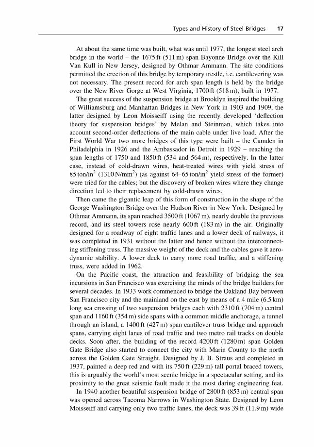
Then came the gigantic leap of this form of construction in the shape of theGeorge Washington Bridge over the Hudson River in New York. Designed byOthmar Ammann, its span reached 3500 ft (1067m), nearly double the previous

record, and its steel towers rose nearly 600 ft (183m) in the air. Originallydesigned for a roadway of eight traffic lanes and a lower deck of railways, it

was completed in 1931 without the latter and hence without the interconnect-ing stiffening truss. The massive weight of the deck and the cables gave it aero-

dynamic stability. A lower deck to carry more road traffic, and a stiffeningtruss, were added in 1962.

On the Pacific coast, the attraction and feasibility of bridging the seaincursions in San Francisco was exercising the minds of the bridge builders for

several decades. In 1933 work commenced to bridge the Oakland Bay betweenSan Francisco city and the mainland on the east by means of a 4 mile (6.5 km)long sea crossing of two suspension bridges each with 2310 ft (704m) central

span and 1160 ft (354m) side spans with a common middle anchorage, a tunnelthrough an island, a 1400 ft (427m) span cantilever truss bridge and approach

spans, carrying eight lanes of road traffic and two metro rail tracks on doubledecks. Soon after, the building of the record 4200 ft (1280m) span Golden

Gate Bridge also started to connect the city with Marin County to the northacross the Golden Gate Straight. Designed by J. B. Straus and completed in

1937, painted a deep red and with its 750 ft (229m) tall portal braced towers,this is arguably the world’s most scenic bridge in a spectacular setting, and itsproximity to the great seismic fault made it the most daring engineering feat.

In 1940 another beautiful suspension bridge of 2800 ft (853m) central spanwas opened across Tacoma Narrows in Washington State. Designed by Leon

Moisseiff and carrying only two traffic lanes, the deck was 39 ft (11.9m) wide


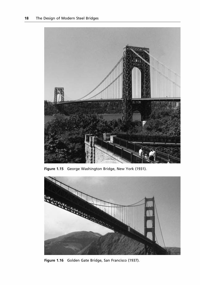
Figure 1.15 George Washington Bridge, New York (1931).

Figure 1.16 Golden Gate Bridge, San Francisco (1937).


and supported on 8 ft (2.4m) deep plate girders rather than a lattice structure.

From the opening, very substantial horizontal and vertical movements of thedeck in wave forms were noticeable even in moderate wind and light traffic,

and earned for the bridge a nickname ‘Galloping Gertie’. Before its construc-tion, tests in a wind tunnel had shown it to be capable of resisting gale forces of

up to 120mile/h (193 km/h). On 7November 1940, a storm that raged for severalhours and reached a speed of 42 mile/h (68 km/h) drove the bridge into an

uncontrollable torsional oscillation, culminating in its collapse into the water.After the great success of long-span bridges in the previous 60 years, this

disaster shook the very foundations of bridge building. The following officialenquiry by three great engineering experts, von Karman, Ammann and GlenWoodruff, blamed no individuals and pointed out no mistakes; it attributed the

failure to a lack of proper understanding and knowledge of the whole profes-sion. The deck was too narrow for the span and thus its torsional rigidity was

inadequate, and the plate girders not only provided insufficient flexural rigid-ity, but their bluff elevation caused wind vortices above and underneath the

deck even in moderate and steady wind speeds.

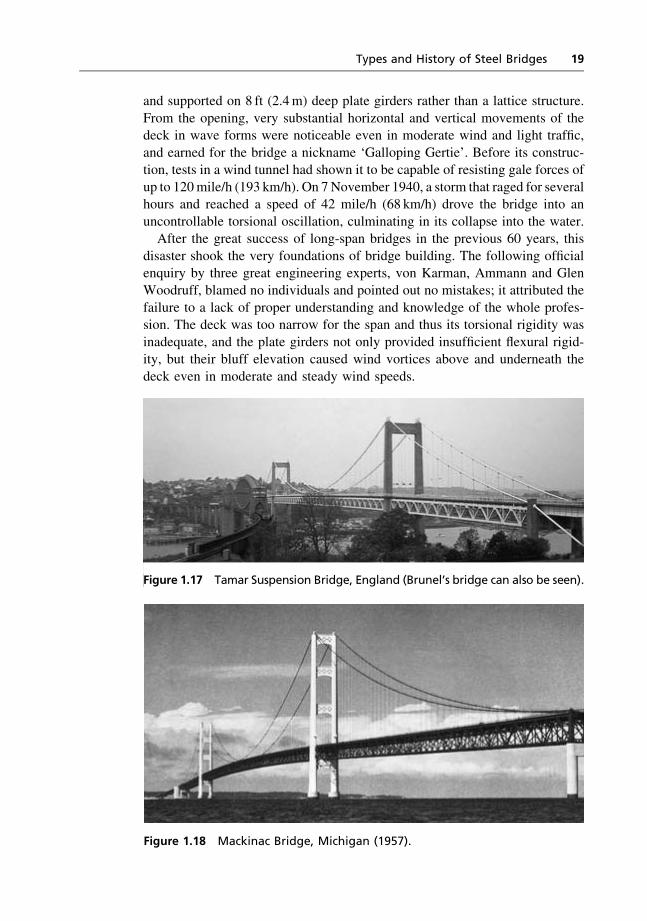
Figure 1.17 Tamar Suspension Bridge, England (Brunel’s bridge can also be seen).

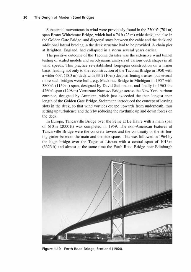
Figure 1.18 Mackinac Bridge, Michigan (1957).


Substantial movements in wind were previously found in the 2300 ft (701m)

span Bronx Whitestone Bridge, which had a 74 ft (23m) wide deck, and also inthe Golden Gate Bridge, and diagonal stays between the cable and the deck and

additional lateral bracing in the deck structure had to be provided. A chain pierat Brighton, England, had collapsed in a storm several years earlier.

The positive outcome of the Tacoma disaster was the extensive wind tunneltesting of scaled models and aerodynamic analysis of various deck shapes in all

wind speeds. This practice re-established long-span construction on a firmerbasis, leading not only to the reconstruction of the Tacoma Bridge in 1950 with

a wider 60 ft (18.3m) deck with 33 ft (10m) deep stiffening trusses, but severalmore such bridges were built, e.g. Mackinac Bridge in Michigan in 1957 with3800 ft (1159m) span, designed by David Steinmann, and finally in 1965 the

4260 ft span (1298m) Verrazano Narrows Bridge across the New York harbourentrance, designed by Ammann, which just exceeded the then longest span

length of the Golden Gate Bridge. Steinmann introduced the concept of leavingslots in the deck, so that wind vortices escape upwards from underneath, thus

setting up turbulence and thereby reducing the rhythmic up and down forces onthe deck.

In Europe, Tancarville Bridge over the Seine at Le Havre with a main spanof 610m (2000 ft) was completed in 1959. The non-American features ofTancarville Bridge were the concrete towers and the continuity of the stiffen-

ing girder between the main and the side spans. This was followed in 1964 bythe huge bridge over the Tagus at Lisbon with a central span of 1013m

(3323 ft) and almost at the same time the Forth Road Bridge near Edinburgh

Figure 1.19 Forth Road Bridge, Scotland (1964).


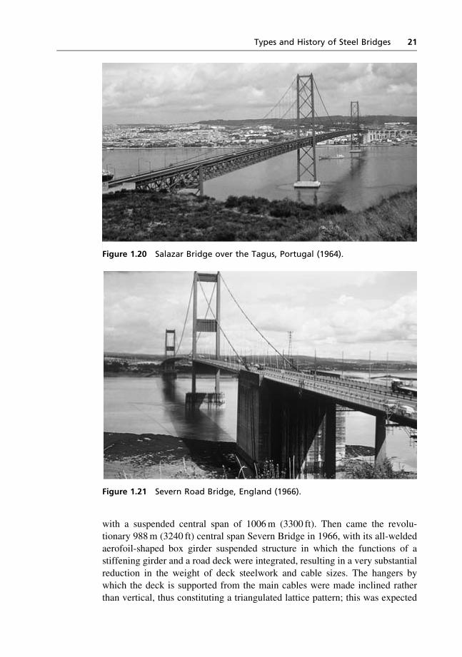
with a suspended central span of 1006m (3300 ft). Then came the revolu-tionary 988m (3240 ft) central span Severn Bridge in 1966, with its all-welded

aerofoil-shaped box girder suspended structure in which the functions of astiffening girder and a road deck were integrated, resulting in a very substantial

reduction in the weight of deck steelwork and cable sizes. The hangers bywhich the deck is supported from the main cables were made inclined rather

than vertical, thus constituting a triangulated lattice pattern; this was expected

Figure 1.20 Salazar Bridge over the Tagus, Portugal (1964).

Figure 1.21 Severn Road Bridge, England (1966).


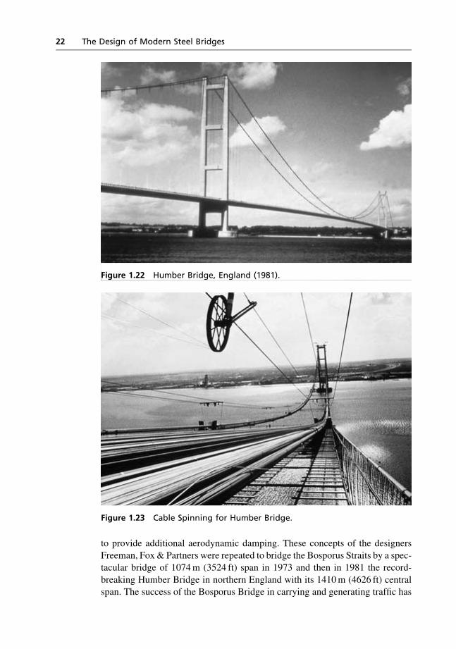
to provide additional aerodynamic damping. These concepts of the designers

Freeman, Fox & Partners were repeated to bridge the Bosporus Straits by a spec-tacular bridge of 1074m (3524 ft) span in 1973 and then in 1981 the record-

breaking Humber Bridge in northern England with its 1410m (4626 ft) centralspan. The success of the Bosporus Bridge in carrying and generating traffic has

Figure 1.22 Humber Bridge, England (1981).

Figure 1.23 Cable Spinning for Humber Bridge.


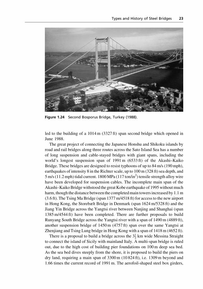
led to the building of a 1014m (3327 ft) span second bridge which opened inJune 1988.

The great project of connecting the Japanese Honshu and Shikoku islands byroad and rail bridges along three routes across the Sato Island Sea has a number

of long suspension and cable-stayed bridges with giant spans, including theworld’s longest suspension span of 1991m (6533 ft) of the Akashi–Kaiko

Bridge. These bridges are designed to resist typhoons of up to 84m/s (190mph),earthquakes of intensity 8 in the Richter scale, up to 100m (328 ft) sea depth, and5m/s (11.2mph) tidal current. 1800MPa (117 ton/in2) tensile strength alloy wire

have been developed for suspension cables. The incomplete main span of theAkashi–KaikoBridgewithstood the greatKobe earthquake of 1995withoutmuch

harm, though the distance between the completedmain towers increased by 1.1m(3.6 ft). The TsingMa Bridge (span 1377m/4518 ft) for access to the new airport

in Hong Kong, the Storebælt Bridge in Denmark (span 1624m/5328 ft) and theJiang Yin Bridge across the Yangtsi river between Nanjing and Shanghai (span

1385m/4544 ft) have been completed. There are further proposals to buildRunyang South Bridge across the Yangtsi river with a span of 1490m (4889 ft),

another suspension bridge of 1450m (4757 ft) span over the same Yangtsi atZhenjiang and Tsing Lung bridge in Hong Kong with a span of 1418m (4652 ft).There is a proposal to build a bridge across the 312 km wide Messina Straight

to connect the island of Sicily with mainland Italy. A multi-span bridge is ruledout, due to the high cost of building pier foundations on 100m deep sea bed.

As the sea bed dives steeply from the shore, it is proposed to build the piers ondry land, requiring a main span of 3300m (10 824 ft), i.e. 1309m beyond and

1.66 times the current record of 1991m. The aerofoil-shaped steel box girders,

Figure 1.24 Second Bosporus Bridge, Turkey (1988).


which have become popular for the deck structure of suspension bridges since

the building of Severn Suspension Bridge in 1966, would require a depth ofabout 10m for the deck structure, as the required depth increases with span.

Such a deck would increase the weight of the deck and the cables and thetowers to such an extent that the feasibility of the project would be threatened.

An alternative solution of ‘slotted’ deck is being investigated, whereby thedeck will have voided longitudinal strips through which wind passing under-

neath the deck escapes upwards through the voids, reducing the lifting forceson the deck. It is proposed that one central aerofoil-shaped box deck will carry

twin rail track, and flanking this box on either side, two aerofoil-shaped boxdecks will each carry three lanes of road. The three boxes will be only 2.25mdeep, will be separated by two 8.0m wide grillage and will be inter-connected

by cross girders of 4.5m depth spanning the whole width of the bridge betweentwo rows of suspension cables. It is hoped that this solution will significantly

reduce the weight of the deck structure and hence of the suspension cables andthe towers.

In cable-stayed bridges the cables are virtually straight between their top atthe tower and their bottom end at the deck where they support the deck

superstructure. Thus, unlike suspension bridge cables, their tension is uniformalong their length and, in this respect at least, they are more efficient. Elimin-ation of substantial anchorages in the ground is another advantage. This type of

bridge construction has become the favourite in the span range of 150–500m,replacing suspension bridges in the higher part of this range.

Cable-stayed bridges are statically indeterminate for structural analysis;each cable stay represents one redundancy. Thus for a three-span bridge, with

one pair of cables supported from each tower top and two vertical cable planes,there will be eight redundancies for the eight cable supports, in addition to the

two represented by the intermediate piers. Historically, several bridges werebuilt in the first half of the nineteenth century, with inclined cable stays

supporting the bridge span. These cables were made from bars and chains andwere not initially tensioned; this allowed large deflections of the deck underloading. This shortcoming led to the concept of combining main suspension

cables of a suspension bridge with a system of inclined cable stays fixedbetween the deck and the towers.

Arnodin in France was a pioneer of a system in which the central portion ofthe span was supported by suspension cables, but the end portions near the

towers were held by cable stays radiating from the towers. The Franz JosephBridge in Prague (1868), the Albert Bridge over the Thames in London (1873),

the Ohio River Bridge at Cincinnati (1867), and the Niagara (1855) andBrooklyn (1883) Bridges by Roebling were examples of the concept ofcombined suspension and cable stay system. The cable stays not only took a

substantial portion of the vertical dead and live loading, but also provided thecrucial aerodynamic stability. The Lezardrieux Bridge over the Trieaux River

in France built in 1925 is the first known example of the modern elegant cable-


stay system, where the cable radiated from the tower tops and transferred their

tension to the stiffening girders.After the Second World War, the need for the reconstruction of the war-

damaged bridges in Europe while building materials were in short supply ledthe designers to this form of construction. In Germany, Dischinger carried out

extensive studies and concluded that cables formed with high strength wires andsubstantially pre-tensioned to support the dead load of the deck would provide

adequate stiffness and aerodynamic stability; it is also essential to achieveaccurate tensioning of the cable along with the desired profiles of the spans

under their dead loads.Dischinger designed and German engineers built the first bridge of this kind,

the Stromsund Bridge in Sweden, opened in 1956, with three spans of 75–183–

75m (246–600–246 ft) and two cable stays radiating from each tower top ineach direction in a fan arrangement along a vertical plane near each edge of the

bridge deck. The stiffening girder consisted of two plate girders along the cableplanes. The width of the navigation channel along the river Rhine often

demanded clear spans of over 250m (820 ft) even during erection, and this newbridge type made this economically possible.

The Theodor Heuss Bridge across the Rhine at Dusseldorf, opened in 1957,had spans of 108–260–108m (354–853–354 ft) and three sets of parallel cablesfrom each tower in each direction, supported from three points in the tower

height in what is now called a harp arrangement. An orthotropic steel deckspanned between the longitudinal girders. This bridge set in motion an impres-

sive variety of cable-stay bridge construction in post-war Germany.The next bridge, the Severins across the Rhine in Koln, opened in 1960 and

became famous for its single A-shaped tower on one bank of the Rhine and twounequal spans of 302 and 151m (991 and 495 ft); it had three pairs of cables on

each side of the tower arranged in a fan shape along inclined cable planes.The third German bridge, across the Elbe River in Hamburg, introduced

the concept, in 1962, of a single cable plane with a central torsionally stiffstiffening girder of box type along the longitudinal axis of the bridge.Then came the classical Leverkusen Bridge across the Rhine in 1964, with a

central cable plane and two cables on each side of two towers in a harp arrange-ment to support three 106–280–106m (348–919–348 ft) spans.

In the late 1960s the introduction of computers for the analysis of redundantstructural systems heralded the multi-cable system of stays, whereby a large

number of small cables attached to the towers at various heights in fan or harpor a combined fashion support the bridge deck at close intervals. This evolu-

tion simplified the construction of each cable and its end connections, reducedthe stiffness requirement of the stiffening girder, which became virtually abeam on continuous elastic supports, and thus increased the span range of this

form of bridge construction.The first of the multi-cable bridges was the Friedrich Ebert Bridge across the

Rhine at Bonn, completed in 1967, with a single cable plane containing 80


cables, supporting a wide box stiffening girder over 120–280–120m (394–

919–394 ft) spans, followed closely by the Rhine Bridge at Rees, with twocable planes and two plate girders as the stiffening girder.

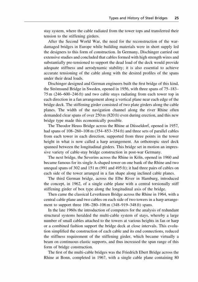
In the Knie Bridge across the Rhine at Dusseldorf, opened in 1969, cables inthe side spans were anchored to the piers underneath; by increasing the

longitudinal rigidity of the whole structure, this innovation enabled the con-

Figure 1.25 Knie Bridge across the Rhine, Dusseldorf, Germany (1969).


struction of a 320m (1050 ft) long span over the river supported by cables fromonly one tower; if supported from two towers, the span could conceivably be

doubled! The same technique was used to build the symmetrical 350m (1148 ft)span Duisburg–Neuenkamp Bridge over the Rhine in 1970.

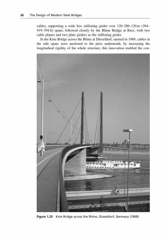
Figure 1.26 Wye Bridge, Wales (1966).

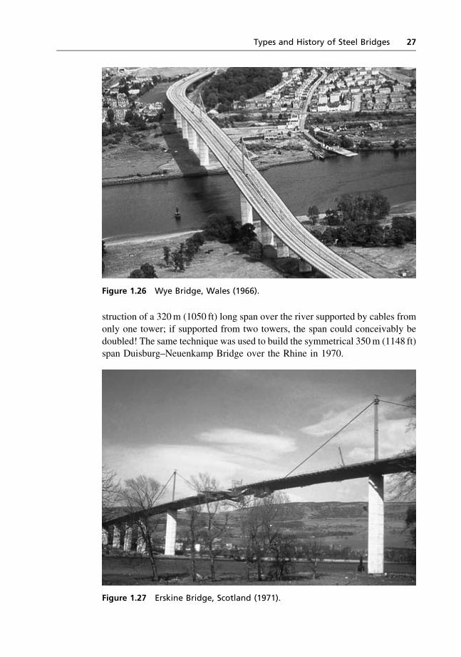
Figure 1.27 Erskine Bridge, Scotland (1971).


The Erskine Bridge in Scotland, opened in 1971, had a large 305m (1000 ft)long span but, following the Wye Bridge design of the early 1960s, employed

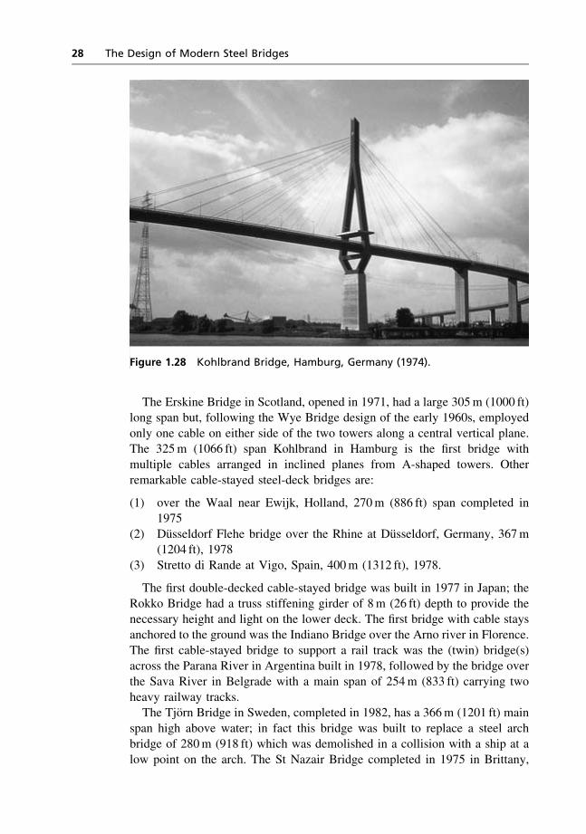
only one cable on either side of the two towers along a central vertical plane.The 325m (1066 ft) span Kohlbrand in Hamburg is the first bridge with

multiple cables arranged in inclined planes from A-shaped towers. Otherremarkable cable-stayed steel-deck bridges are:

(1) over the Waal near Ewijk, Holland, 270m (886 ft) span completed in1975

(2) Dusseldorf Flehe bridge over the Rhine at Dusseldorf, Germany, 367m(1204 ft), 1978

(3) Stretto di Rande at Vigo, Spain, 400m (1312 ft), 1978.

The first double-decked cable-stayed bridge was built in 1977 in Japan; theRokko Bridge had a truss stiffening girder of 8m (26 ft) depth to provide thenecessary height and light on the lower deck. The first bridge with cable stays

anchored to the ground was the Indiano Bridge over the Arno river in Florence.The first cable-stayed bridge to support a rail track was the (twin) bridge(s)

across the Parana River in Argentina built in 1978, followed by the bridge overthe Sava River in Belgrade with a main span of 254m (833 ft) carrying two

heavy railway tracks.The Tjorn Bridge in Sweden, completed in 1982, has a 366m (1201 ft) main

span high above water; in fact this bridge was built to replace a steel archbridge of 280m (918 ft) which was demolished in a collision with a ship at a

low point on the arch. The St Nazair Bridge completed in 1975 in Brittany,

Figure 1.28 Kohlbrand Bridge, Hamburg, Germany (1974).


France, has a central span of 404m (1325 ft), and Faro Bridge in Denmark,

completed in 1985, has a 295m (968 ft) span. The Luling Bridge across theMississippi near New Orleans, opened in 1984, has a 25m (82 ft) wide steel

orthotropic deck on a trapezoidal box girder, supported by 12 cable stays fromeach A-frame tower, with a 376m (1235 ft) central span. The Meiko Nishi

Bridge in Japan, completed in 1985, has a 405m (1329 ft) span.The Annacis Bridge in Vancouver, Canada, and the Dao Kanong Bridge in

Bangkok, Thailand, were opened in 1987 and had central spans of 465 and450m (1526 and 1476 ft), respectively. Since then the Tampico Bridge in

Mexico with 360m (1181 ft) span, the Hoogly Bridge in Kolkata, India(renamed ‘Vidyasagar Setu’) with 457m (1500 ft) span, the Yokohama BayBridge in Japan with 460m (1509 ft) span to carry 12 lanes of traffic on two

decks, the Queen Elizabeth II Bridge over the Thames at Dartford near London(450m/1476 ft span), the Second Severn Crossing 5 km downstream of the

Severn Suspension Bridge (465m/1526 ft span), and the Oresund Bridgebetween Sweden and Denmark with a span of 490m (1608 ft) have been

completed. The Honshu–Shikoku Bridge Project has a fascinating pair ofcable-stayed bridges located end-to-end with 185–420–185m (607–1378–

607 ft) spans to carry roadway on the upper deck and railway on the lower:there is also another bridge called Ikuchi with 150–490–150m (492–1608–492 ft) spans.

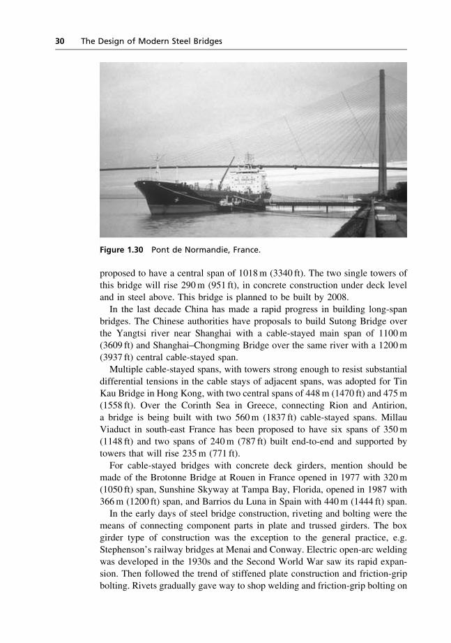
Then, in 1995, came a gigantic leap in span length of cable-stayed bridges inthe form of Pont de Normandie across the Seine near Honfleur in France with a

cable-stayed span of 816m (2677 ft). But this record was overtaken in 1999 bythe completion of Tatara Bridge across Seto Sea in Japan with a 890m

(2920 ft) cable-stayed span. Even this record will be bettered by the proposedStonecutters Bridge over the Rambles Channel in Hong Kong which is

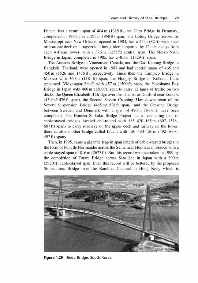
Figure 1.29 Jindo Bridge, South Korea.


proposed to have a central span of 1018m (3340 ft). The two single towers ofthis bridge will rise 290m (951 ft), in concrete construction under deck leveland in steel above. This bridge is planned to be built by 2008.

In the last decade China has made a rapid progress in building long-spanbridges. The Chinese authorities have proposals to build Sutong Bridge over

the Yangtsi river near Shanghai with a cable-stayed main span of 1100m(3609 ft) and Shanghai–Chongming Bridge over the same river with a 1200m

(3937 ft) central cable-stayed span.Multiple cable-stayed spans, with towers strong enough to resist substantial

differential tensions in the cable stays of adjacent spans, was adopted for TinKau Bridge in Hong Kong, with two central spans of 448m (1470 ft) and 475m(1558 ft). Over the Corinth Sea in Greece, connecting Rion and Antirion,

a bridge is being built with two 560m (1837 ft) cable-stayed spans. MillauViaduct in south-east France has been proposed to have six spans of 350m

(1148 ft) and two spans of 240m (787 ft) built end-to-end and supported bytowers that will rise 235m (771 ft).

For cable-stayed bridges with concrete deck girders, mention should bemade of the Brotonne Bridge at Rouen in France opened in 1977 with 320m

(1050 ft) span, Sunshine Skyway at Tampa Bay, Florida, opened in 1987 with366m (1200 ft) span, and Barrios du Luna in Spain with 440m (1444 ft) span.

In the early days of steel bridge construction, riveting and bolting were themeans of connecting component parts in plate and trussed girders. The boxgirder type of construction was the exception to the general practice, e.g.

Stephenson’s railway bridges at Menai and Conway. Electric open-arc weldingwas developed in the 1930s and the Second World War saw its rapid expan-

sion. Then followed the trend of stiffened plate construction and friction-gripbolting. Rivets gradually gave way to shop welding and friction-grip bolting on

Figure 1.30 Pont de Normandie, France.


site. Erection methods of launching and cantilevering were widened by the

development of floating-out techniques and heavy lifting equipment suitablefor handling entire structures in one piece.

Post-war years also saw a great expansion of the understanding of structuralbehaviour and analysis of indeterminate interconnected structural systems. The

state-of-the-art before the war generally consisted of assuming pin-jointedconnections between different structural elements and manually solving simul-

taneous equations. In the aftermath of the war devastations, the knowledge andexperience of the aircraft industry was imported into bridge building in order to

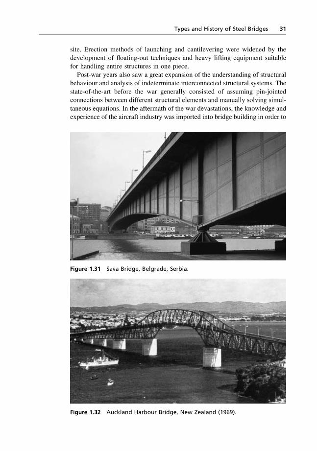
Figure 1.31 Sava Bridge, Belgrade, Serbia.

Figure 1.32 Auckland Harbour Bridge, New Zealand (1969).


provide the expertise necessary for rebuilding thousands of demolished bridgeswith minimum amounts of scarce construction materials like steel. This

brought in the understanding of torsional behaviour of thin-walled closedsections, and many of the mathematical tools for solving complex analytical

problems. This was followed by the advent of electronic computers whichvastly increased the facilities for structural analysis. Highly indeterminate

structural systems could now be analysed in minutes and it was no longernecessary to make assumptions like pinned joints. One immediate benefit was

the improved lateral distribution of concentrated loads over the whole width ofthe bridge deck. Orthotropic steel decks became the favourite type of light-

weight economical bridge construction over 500 ft (150m) spans. The torsionalstiffness of single or multiple cell box girders proved highly advantageous inthe ‘cantilever’ type erection method over great heights or wide rivers. The

Dusseldorf–Neuss Bridge across the Rhine, with 103–206–103m (338–676–338 ft) span box girders with a steel orthotropic deck and completed in 1951,

set this modern trend. The Sava Road Bridge in Belgrade, Yugoslavia, withcontinuous plate girders of 856 ft (261m) centre span completed in 1956 was

another landmark. In box girders with orthotropic top flange, each elementfunctioned in multiple ways, e.g. the flange stiffeners carried the wheel loads

and also acted as the tension/compression flange of the box girder; this led togreat economy of material. Great examples of this form of construction, withtheir maximum span length and year of completion, are:

� Zoo Bridge, Koln, Germany, 850 ft (259m) 1966

� Charlotte Bridge, Luxembourg, 768 ft (234m) 1966

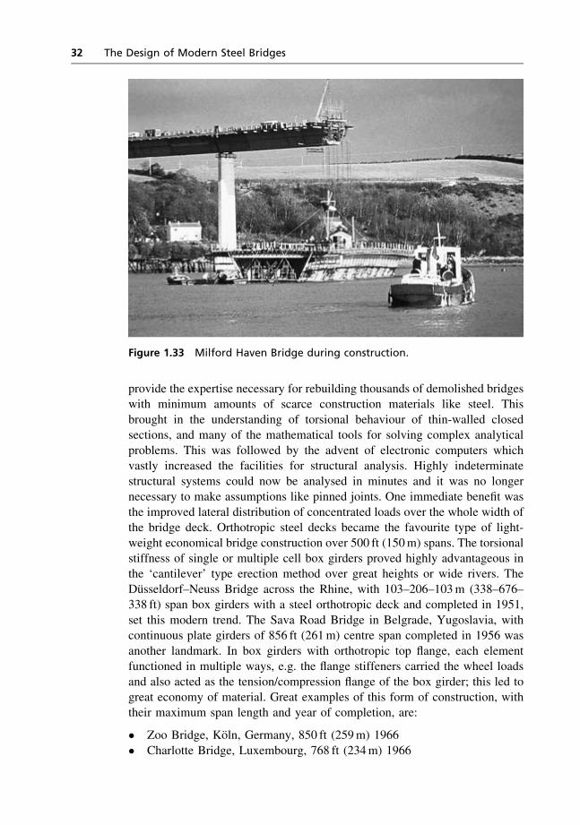
Figure 1.33 Milford Haven Bridge during construction.


� San Mateo Hayward, San Francisco, 750 ft (229m) 1967� Auckland Harbour, New Zealand, 800 ft (244m) 1969

� Gazelle, Belgrade, Serbia, 820 ft (250m) 1970.

The 250m (820 ft) high, 376m (1234 ft) span motorway bridge over theSfalasse Valley in Calabria, Italy, with two inclined portal legs that divided the

Figure 1.34 Avonmouth Bridge, England.

Figure 1.35 Europa Bridge, Italy.


Figure 1.36 Foyle Bridge, Northern Ireland.

Figure 1.37 A motorway bridge at Brentwood, England.

Figure 1.38 Windmill Bridge, Newark, England.


span into 110–156–110m (361–512–361 ft), completed in the early 1970s, was

another striking example of steel box girder orthotropic deck construction.However, the systematic and confident progress with light and rapid

construction of steel bridges suffered a big jolt in the early 1970s, with the

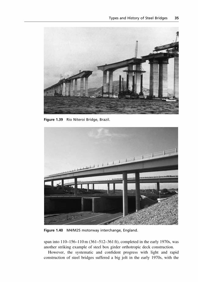
Figure 1.39 Rio Niteroi Bridge, Brazil.

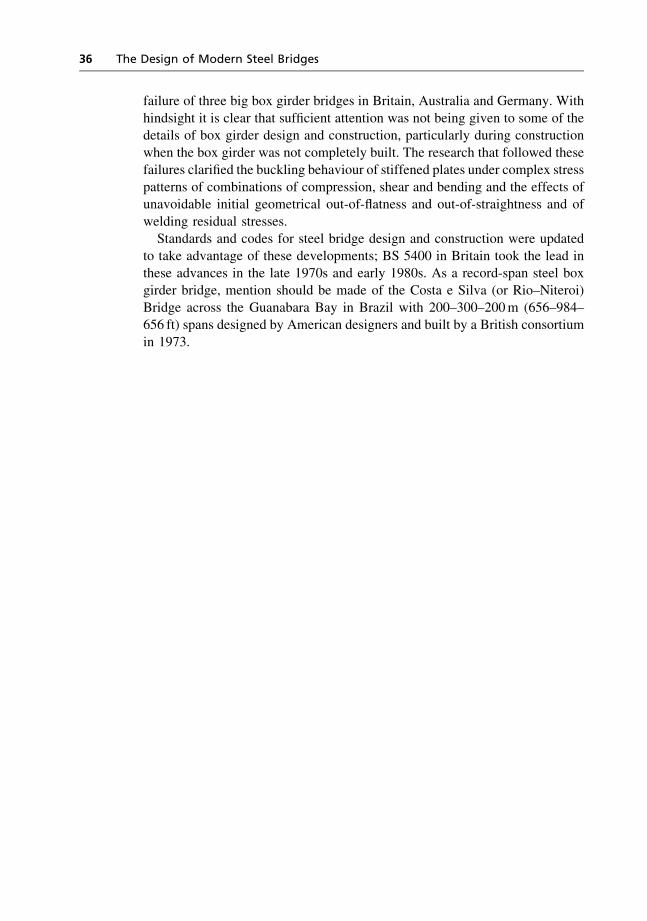
Figure 1.40 M4/M25 motorway interchange, England.


failure of three big box girder bridges in Britain, Australia and Germany. With

hindsight it is clear that sufficient attention was not being given to some of thedetails of box girder design and construction, particularly during construction

when the box girder was not completely built. The research that followed thesefailures clarified the buckling behaviour of stiffened plates under complex stress

patterns of combinations of compression, shear and bending and the effects ofunavoidable initial geometrical out-of-flatness and out-of-straightness and of

welding residual stresses.Standards and codes for steel bridge design and construction were updated

to take advantage of these developments; BS 5400 in Britain took the lead inthese advances in the late 1970s and early 1980s. As a record-span steel boxgirder bridge, mention should be made of the Costa e Silva (or Rio–Niteroi)

Bridge across the Guanabara Bay in Brazil with 200–300–200m (656–984–656 ft) spans designed by American designers and built by a British consortium

in 1973.


Chapter 2

Types and Properties of Steel

2.1 Introduction

Steel used for building bridges and structures contains:

(1) iron(2) a small percentage of carbon and manganese

(3) impurities that cannot be fully removed from the ore, namely sulphur andphosphorus

(4) some alloying elements that are added in very small quantities to improve

the properties of the finished product, namely copper, silicon, nickel,chromium, molybdenum, vanadium, columbium and zirconium.

The strength of the steel increases as the carbon content increases, but some other

properties like ductility and weldability decreases. Sulphur and phosphorus haveundesirable effects and hence their maximum amount is controlled. Steel used

for building bridges may be grouped into the following three categories:

(1) Carbon steels – only manganese, and sometimes a trace of copper andsilicon, are used as alloying elements. This is the cheapest steel available forstructural uses where rigidity rather than strength is important. It comes with

yield stress up to 275N/mm2 and can be easily welded. The Euronorm EN10025 steels to grades S235 and S275, and the North American steels to

grade 36 of AASHTO M270 and ASTM A709 and earlier ASTM A36 belongto this category.

(2) High-strength steels – these cover steels of a wide variety with yield

stress in the range of 300 to 390N/mm2. They derive their higher strength andother required properties from the addition of alloying elements mentionedearlier. The Euronorm EN 10025 steels to grade S355, and the North American

steels to grade 50 of AASHTO M270 and ASTM A709, and earlier ASTMA572 belong to this category.

(3) Heat-treated carbon steels – these are the steels with the highest

strength, and still retain all the other properties that are essential for buildingbridges. They derive their enhanced strength from some form of heat treatment

after rolling, namely normalisation or quenching-and-tempering. The European

37

EN 10113 steels to grades S420 and S460 and the North American steels to

grade 100 of AASHTO M270 and ASTM A709 and earlier ASTM A514belong to this category.

(4) Weathering steel – this variety of steel is produced with enhanced

resistance to atmospheric corrosion and these can be left unpainted in appropriatesituations. In Europe this steel is produced to Euronorm EN 10155 and comes in

two grades of S235 and S355. In North America they are produced to grades50W, 70W and 100W of AASHTOM270 and ASTMA709. Steel of this varietyconforming to earlier ASTM A588 is known by the trade name ‘corten’ steel.

2.2 Properties

The properties of structural steel relevant for its use in bridge construction arethe following:

(1) strength

(2) ductility(3) weldability

(4) notch toughness(5) weather resistance.

The strength properties of commonly available structural steels arerepresented in the idealised tensile stress–strain behaviour in Fig. 2.1(a). The

slope of the initial linear part is defined as Young’s modulus E. At a stress justbeyond the limit of linearity, the flow of the steel becomes plastic at nearly

constant stress. This stress is called the yield stress (or yield point) Re of thesteel. After the yield is completed the stress increases again until the maximum

stress, called the tensile strength (Rm) is reached. With further straining largelocal elongation and reduction in cross-section occur, and the stress falls until

fracture takes place.With some steel, after the initial limit of linearity, the stress may attain a

maximum, then fall and remain approximately constant during yielding, as

shown in Fig. 2.1(b); the value of the stress at the commencement of yield iscalled the upper yield stress ReH. Some steel does not show the yield

phenomenon; beyond the limit of linearity, the strain continues to increasenon-proportionally, as shown in Fig. 2.1(c). In such cases a ‘proof stress’ is

measured. Proof stress (total elongation) Rt is measured by drawing a lineparallel to the stress axis and distant from it by the required total elongation;

proof stress (non-proportional elongation) Rp is measured by drawing a lineparallel to the initial straight portion of the behaviour and distant from it by therequired non-proportional elongation. For such steel a 0.5% total elongation

proof stress is regarded as the yield stress. Unloading from any stage of initialstraining occurs along a line approximately parallel to the initial straight

portion of the stress–strain curve.


2.3 Yield stress

The yield stress is the most important strength parameter of structural steel.

Yield stress is normally measured in tension only. Such measurements areaffected by the specimen geometry, the rate of straining, location and orienta-

tion of the specimen in the rolled section or plate and the stiffness of the testingmachine. A higher rate of straining increases the yield stress and the tensile

strength. Various national and international standards specify these testing

Figure 2.1 Idealised stress–strain behaviour of steel.

Types and Properties of Steel 39

parameters; for example, for the determination of yield stress British Standard

BS 18[1] limits the rate of straining at the time of yielding to 0.0025 persecond; when this cannot be achieved by direct control, the initial elastic

stressing rate has to be controlled within the values stipulated for differenttesting machine stiffnesses.

Within a zone of, say, 50mm from a rolled edge, yield stress may be up to15% higher than in the remainder of a plate. Yield stress in the transverse direc-

tion may be approximately 212% less than in the longitudinal direction of rolling.The yield stress (and also the tensile strength) varies with the chemical

composition of the steel, the amount of mechanical working that the steelundergoes during the rolling process and the heat treatment and/or coldworking applied after rolling. Thinner sections produced by an increased

amount of rolling have higher yield stresses; even in one cross-section of arolled section the thinner parts have higher yield stresses than the thicker parts.

Heat treatment or cold working may remove the yield phenomenon.The stress–strain behaviour under compression is normally not determined

by tests and is assumed to be identical to the tensile behaviour. In reality thecompressive yield stress may be approximately 5% higher than the tensile

yield stress. The state of stress at any point in a structural member may be acombination of normal stresses in orthogonal directions plus shear stresses inthese planes. Several classical theories for yielding in three-dimensional stress

states have been postulated; the theory that has been found most suitable forductile material with similar strength in compression and tension is based on

the maximum distortion energy and attributed variously to Huber, von Misesand Hencky. According to this theory, in a two-dimensional stress state yield-

ing takes place when normal stresses s1 and s2 on the two orthogonal planesand shear stress t on these planes satisfy the following condition:

s21 þ s2

2 � s1s2 þ 3t2 ¼ s2y

where sy is the measured yield stress of the material. It may be noted that,according to this theory: (i) the yield stress ty in pure shear, i.e. without any

normal stresses, is equal to sy/ffiffiffi3

pand (ii) in the biaxial stress state, the normal

stress in one direction may reach values higher than the measured uniaxial

yield stress sy before yielding takes place; e.g. if s1¼ 2s2, yielding will nottake place until s1 reaches approximately 15% higher than the uniaxial yield

stress of the material.The other elastic properties that influence the state of stress at any point are:

(1) Young’s modulus E, which is in the range 200 to 210 kN/mm2.(2) The shear modulus or modulus of rigidity G, which is the ratio between

shearing stress and shear strain and is in the range 77 to 80 kN/mm2.(3) Poisson’s ratio m, which is the ratio between lateral strain and longi-

tudinal strain caused by a longitudinally applied stress and is usuallytaken as 0.3 for structural steel.


(4) The coefficient of thermal expansion which is the expansion/contraction

per unit length caused by one degree change in the temperature and isnormally taken as 12�10�6/�C.

There is a theoretical relationship between E, G, and m, given by G¼E/{2(1þ m)}.

2.4 Ductility

Ductility of a material is measured by its capacity to undergo large strains afterthe onset of yielding and before fracture. This property enables a structure to

exhibit large deformation when the load it carries exceeds the value corres-ponding to its yield stress, thus providing an advance warning of possiblefailure.

In a structure with redundancy, i.e. alternative load paths, when yield strain isexceeded in a critical component, this property enables it to redistribute the

excess load to other components while the critical component retains its yieldload. In a tensile test, after the maximum load, i.e. tensile strength Rm (see

Fig. 2.1(a)), is reached, necking occurs in one cross-section, accompanied bylarge local elongation.

After fracture, the two pieces are held together to measure the totalpermanent elongation of the original gauge length. This elongation represents

the ductility of the material. However, it is affected by the geometricalparameters of a test piece, e.g. cross-sectional shape and gauge length. Byinternational agreement, the relationship between gauge length Lo and cross-

sectional area So in the gauge length of tensile test pieces has been establishedas Lo¼ 5.65

ffiffiffiffiffiSo

p. However, other gauge lengths are often used, e.g. 200mm or

8 inches are quite common in the UK and USA, respectively. Structural steelspecifications prescribe a minimum value of this percentage elongation, in the

range of 17 to 26%.Good ductility through the thickness of thick rolled products is necessary to

prevent lamellar tearing when high stresses occur in the direction of thethickness.

2.5 Notch ductility

Notch ductility is a property of metals indicating their resistance to brittlefracture. Brittle fracture is a form of failure that occurs suddenly under a load

well below the level to cause yielding. It is initiated by the existence of a smallcrack or other form of notch. Very high concentration of stress occurs at the

root of a natural crack. Any sudden change in the cross-section of a loadedmember has a notch-like effect, namely it disturbs the stress pattern and causes


a local stress concentration. If the local yielding at the tip of the crack or notch

is insufficient to spread the load over a large area, a brittle fracture may beinitiated. Once initiated, the fracture propagates at high speed driven by the

release of the elastic strain energy in the structure.Design should avoid any sharp geometrical discontinuity, change of section

and re-entrant angles. Workmanship should avoid accidental notches like dents,pitting and various weld defects, namely undercutting, slag inclusions, porosity

or cracks.Brittle fracture is more likely to occur at low temperatures, as the notch

ductility of steel falls with decreasing temperature. Sometimes a temperaturechange of a few degrees changes the ductility so substantially that there is atransition from a ductile to brittle type behaviour.

Brittle fracture is more likely in a massive structural component than a lightone. This is due to the three-dimensional stress conditions in thick elements

and the likelihood of non-metallic inclusions, segregation or lamination left inthick rolled products.

Welded steelwork has more propensity to brittle fracture than unweldedsteelwork, as welding may:

(1) introduce defects

(2) reduce the notch ductility of the heat-affected zone near the weld(3) introduce weld metal of different notch ductility

(4) leave substantial residual stresses, particularly tensile stresses as high asyield stress near the welds.

Flame cutting also produces defects and reduces ductility in the hardenedheat-affected zone.

Other factors that increase susceptibility to brittle fracture are:

(1) cold working during the fabrication process, namely bending, shearing,etc., particularly in higher strength steels

(2) ‘hot dip’ galvanising(3) impact loading

(4) unsuitable heat treatment(5) large amount of non-metallic alloying elements in the steel.

There is no single measurable property of structural steel by which itssusceptibility to brittle fracture can be uniquely measured. The test that is

commonly used nowadays is called the Charpy V-notch impact test. In this testa specimen is hit by a striker mounted on the end of a pendulum. The striker islifted initially to a specified height and then released to hit and break the

specimen, swinging and rising to a height on the other side. The differencebetween the two heights, multiplied by the mass of the striker, is the energy

absorbed in fracturing the specimen. The specimen has a notch at the point ofmaximum tensile stress, and is held at a specified temperature.


The theory of fracture mechanics seeks to explain the static strength of a

component in terms of the size of a pre-existing notch or flow. This theory wasoriginally restricted to elastic stress conditions in thin sheets, i.e. without any

stress in the through-thickness direction, but has been extended more recentlyto thick plates in which the strain, but not the stress, through the thickness is

negligible, and also to allow for yielding or plastic deformation before fracture.The fracture mechanics theory attempts to establish a relationship between the

fracture toughness of the material, the permitted size of the initial crack or flawand the permitted stress level.

In the latest revision of the British Standard BS 5400 Part 3[2] for steelbridges, the minimum notch ductility requirements have been specified as:

(a) U5T� 20 and

(b) t4 50K (355/sy)1.4 (1.2)(U�T)/10

where U is the design minimum temperature of the structural part under

consideration in centigrade: this could be several degrees lower than theminimum ambient air temperature around the bridge; T is the test temperature

in centigrade at which a minimum Charpy energy of 27 J is specified for thematerial for standard longitudinal V-notch test pieces; t is the maximumpermitted thickness of the part in millimetres; K is the coefficient which is the

product of the four following factors, i.e. K¼ kdkgksks, in which kd depends onthe nature of the potential fracture initiation site and varies from 0.5 to 2.0; kgdepends on any gross stress concentration due to geometrical discontinuity likeopen holes or re-entrant corners; kg can be taken as k� 0.5 when k is the ratio of

peak principal tensile stress to nominal principal tensile stress at the discon-tinuity. kg could vary from 0.5 to 1.0; ks depends on the level of applied stress

at the ultimate limit state; it varies from 1.0 when the applied stress is greaterthan 0.5sy in tension to 2.0 when the applied stress is compressive; ks depends

on the rate of loading; it varies from 0.5 for structural members that can bedirectly hit by an impact loading (like a parapet post or a column close totraffic), to 1.0 for bridge girders underneath a carriageway; sy is the yield

stress of the steel material in N/mm2. Take the example of a highly stressedbridge girder tension flange made of steel with sy¼ 275N/mm2 and specified

Charpy energy of 27 J at �20�C. The factor kd is taken as 0.7 due to thepresence of a transverse butt weld; each of the other three factors kg, ks and ksis 1.0. The design minimum temperature U of the tension flange is �24�C. Themaximum permitted thickness of the tension flange will be

50� 0:7� ð355=275Þ1:4 � 1:20ð�24þ20Þ=10 ¼ 46:53mm

In most countries, structural steel for each level of yield stress is produced inseveral grades of Charpy energy absorption. These grades are either in anincreasing order of energy value for the same test temperature or constant


energy value for decreasing levels of test temperatures or a mixture of both.

Unfortunately no unique relationship exists between energy values at differenttest temperatures.

The AASHTO specification categorises structural steel materials into twocategories: FCM (fracture-critical material) and non-FCM; the material of a

component is defined as FCM if its fracture would cause collapse of thestructure. The specification also categorises the bridge sites into three

temperature zones as follows:

The specified toughness requirements are higher with colder zones, thickercomponents, higher grades of steel and fracture-critical components. The

Charpy energy requirements vary from 20 J at 21�C testing temperature fornon-FCM components of grade 36 steel upto 38mm thick in temperature zone1, to 41 J at �23�C for FCM component of grade 70W steel upto 63mm thick

in temperature zone 3.

2.6 Weldability

Steels with carbon content less than about 0.30% are weldable, provided

suitable welding processes and electrodes are used. This includes all thecategories of steel used for building bridges and mentioned in Section 2.1.

However, even for these steels, ease of weldability varies. Increased amountsof carbon and manganese, which are necessary for higher strengths, make the

steel harder and consequently more difficult to weld. The group of alloyingelements, chromium, molybdenum and vanadium, which are added to further

increase the strength, and the elements nickel and copper which are added toimprove weathering resistance, also reduce weldability. For the purpose of

measuring weldability, a term ‘carbon equivalent’ is used, which is given bythe following formula

CþMn

6þ CrþMoþ V

5þ Niþ Cu

15

where C, Mn, etc. represent the percentage of the element concerned in the

chemical composition of the steel. The chemical composition of steel, i.e. thepercentage content of the various alloying elements, is usually checked by

ladle analysis. Chemical analysis may also be done on the finished product

Temperature zone For minimum service temperature

1 Above �18�C2 �18�C to �34�C3 �35�C to �51�C


itself, but some deviations as stipulated in the specifications are then permitted

from the specified composition limits. Higher yield stresses can only beobtained by increasing the percentage content of the various alloying elements,

thus increasing the carbon equivalent value. Hence welding of higher strengthsteels is more difficult. Maximum values for carbon equivalent are sometimes

given in the specifications. Steels with carbon equivalent values higher than0.53 are likely to require special measures in welding. Welding difficulties also

increase with thicker members and increased restraint against shrinkage due tocooling. If the cooling rate is too rapid, excessive hardening and cracking may

occur in the weld and the heat affected zone: this can be avoided by controllingweld run dimensions in relation to material thickness, by applying pre-heatand controlling interpass temperature between weld runs and by using low-

hydrogen electrodes.

2.7 Weather resistance

A special type of steel has been developed for increased resistance to corrosion –this is called ‘weathering steel’. When used in the appropriate environment,this steel forms a thin iron oxide film on the surface. This film is a tightly

adherent coating that resists any further rusting by preventing the ingress ofmoisture. Alternate drying and wetting is the ideal condition for the formation

and durability of this film. Under bridges in countries like Britain, the environ-ment is usually damp most of the time, and this film comes off and is reformed

at intervals of one to three years. Weathering steel bridges can be leftunpainted if the colour of the oxide coating is aesthetically acceptable – it

varies from red–orange to purple–brown. InBritain, theDepartment of Transportspecifies[3] an additional sacrificial thickness of one or two millimetres oneach surface, depending on the sulphur content in the atmosphere; unpainted

weathering steel is not permitted: (i) in a marine environment, (ii) where it canbe subjected to de-icing salt spray and (iii) in locations with very high atmos-

pheric sulphur content. In the United States, weathering steel is known by tradenames like Mayri R (Bethlehem Steel) and Cor-ten (United States Steel).

Higher corrosion resistance of weathering steel is achieved by addingchromium, copper and sometimes nickel as alloying elements; as a result the

carbon equivalent value is higher, thus requiring special measures in welding.

2.8 Commercially available steels

The material properties of some commercially available steel to variousnational/international specifications and suitable for use in steelwork for bridge

structures are given in Table 2.1. The following notes apply to their properties


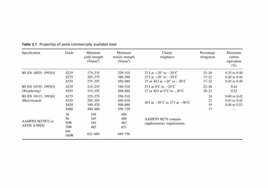
Table 2.1 Properties of some commercially available steel

Specification Grade Minimumyield strength(N/mm2)

Minimumtensile strength

(N/mm2)

Charpytoughness

Percentageelongation

Maximumcarbon

equivalent(%)

BS EN 10025: 1993[4] S235 175–235 320–510 27 J at þ20� to �20�C 21–26 0.35 to 0.40S275 205–275 380–580 27 J at þ20� to �20�C 17–22 0.40 to 0.44S355 275–355 450–680 27 or 40 J at þ20� to �20�C 17–22 0.45 to 0.49

BS EN 10155: 1993[5](Weathering)

S235S355

215–235315–355

340–510490–680

27 J at 0�C to �20�C27 or 40 J at 0�C to �20�C

22–2618–22

0.440.52

BS EN 10113: 1993[6](Heat-treated)

S275S355

225–275295–355

350–510450–630

2422

0.40 to 0.420.43 to 0.45

S420 340–420 500–68040 J at �20�C to 27 J at �50�C

19 0.48 to 0.52S460 400–460 550–720 17 –

AASHTO M270[7] orASTM A709[8]

3650

248345

400448 AASHTO M270 contains

supplementary requirements50W 345 48370W 483 621100

621–689 689–758100W

given in this table:

(1) Western European Steel:

(a) EN 10025 covers commonly used steel for welded, bolted or rivetedstructures for service at ambient temperature. EN 10155 covers

weathering steel for similar applications. EN 10113 covers steelsuitable for heavily loaded structures for service at low temperatures;

it has better notch toughness values and lower carbon percentage andcarbon equivalent values.

(b) According to the definitions given in Section 2.1, steel grades

designated S235 and S275 are weldable carbon steel; S355 weldablehigh strength steel, and S420 and S460 heat-treated carbon steel.

(c) Each grade of steel to EN 10025 and 10155 is suffixed by qualitydesignations JR, JO, J2 and K2 which are for successively higher

qualities in Charpy toughness and weldability. Additional qualitydesignations G1–G4 represent the deoxidation process, N represents

normalised steel and C represents suitability for cold forming.(d) EN 10113 steels come with two minimum Charpy toughness values

of 40 J at �20�C and 27 J at �50�C; they also come in two deliveryconditions of ‘normalised’ and ‘thermo-mechanically rolled’,designated by N and M respectively; the latter steel has lower carbon

percantage and carbon-equivalent values.(e) Some steel grades may not have guaranteed maximum carbon-

equivalent values and/or notch toughness and/or minimum percen-tage elongations; they should be used in welded bridge structures

only after further bridge-specific testing.(f) In each grade of steel, the minimum yield strength, the minimum

tensile strength and the minimum percentage elongation require-ments reduce with increasing thickness of the product within therange shown in the table. Hence additional caution is needed for

using very thick products.(g) E grade steel to EN 10025 may not be suitable for welded bridge

structures, as it does not have guaranteed maximum carbon per-centage and minimum Charpy toughness values.

(2) North American Steel:(a) Steel to AASHTO designation M270 grades 36, 50, 50W and 70W

are suitable for welded bridge structures; suffix W in the graderepresents weathering steel. Steel to grades 100 and 100W have a

rather narrow margin between yield stress and minimum strength inpercentage terms, and hence structures built with such steel may notpossess the post-yielding reserve of strength before collapse that can

be expected from structures built with lower grade steels.(b) ASTM A709 steels are equivalent to AASHTO M270 steels of

identical grades with respect to yield strength and minimum strength.


AASHTO M270 specification includes mandatory notch ductility

and weldability requirements, thus pre-qualifying steel to thisspecification for use in welded bridges. But ASTM A709 does not

contain mandatory notch ductility and weldability requirements andhence steel to this specification must satisfy bridge-specific

requirements for notch ductility and weldability.(c) The following equivalence between steels of different grades to

AASHTO M270 or ASTM A709 and steel to older specificationsmay be noted:

2.9 Recent developments

The off-shore structures in the North Sea have given rise to higherrequirements on structural steel than any other previous applications – due

to the great water depths, huge wave forces and low temperatures encounteredthere. High-strength carbon-manganese steel has been improved to obtain yield

stresses up to 500N/mm2 by the addition of very small quantities of alloyingelements like niobium, vanadium, nickel, copper and molybdenum.

Quenching with pressurised water and tempering have been used to furtherimprove the mechanical properties, with minimum yield stresses in the regionof 700N/mm2 and good ductility, weldability and notch toughness properties.

References

1. British Standard BS 18: 1971. Method for tensile testing of metal: Part 2: Steel

(General). British Standards Institution, London.

2. British Standard BS 5400: Part 3: 2000: Code of Practice for Design of Steel

Bridges. British Standards Institution, London.

3. Departmental Standard BD 7/81: Weathering Steel for Highway Structures.

Department of Transport, London.

4. British Standard BS EN 10025: 1993. Hot rolled products of non-alloy structural

steels. Technical Delivery Conditions. British Standards Institution, London.

5. British Standard BS EN 10155: 1993. Structural steels with improved atmospheric

corrosion resistance. Technical Delivery Conditions. British Standards Institution,

London.

AASHTO M270 orASTM A709 grades

Older ASTMspecifications

36 A3650 A57250W A58870W A852100, 100W A514


6. British Standard BS EN 10113: 1993. Hot rolled products in weldable fine grain

structural steels. British Standards Institution, London.

7. (a) AASHTO Standard Specification for Highway Bridges: 1996

(b) AASHTO LRFD Bridge Design Specification: 1998

(c) AASHTO LRFD Bridge Construction Specification: 1998

American Association for State Highway and Transportation Officials. Washing-

ton, DC.

8. ASTM Designation A709M: Standard Specification for Carbon and High-strength

Low-alloy Structural Steel Shapes, Plates and Bars and Quenched-and-Tempered

Alloy Structural Steel Plates for Bridges: October 2001. ASTM International, West

Conshohocken, PA, USA.


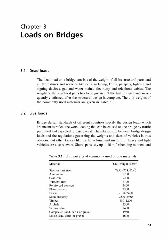
Chapter 3

Loads on Bridges

3.1 Dead loads

The dead load on a bridge consists of the weight of all its structural parts and

all the fixtures and services like deck surfacing, kerbs, parapets, lighting andsigning devices, gas and water mains, electricity and telephone cables. The

weight of the structural parts has to be guessed at the first instance and subse-quently confirmed after the structural design is complete. The unit weights of

the commonly used materials are given in Table 3.1.

3.2 Live loads

Bridge design standards of different countries specify the design loads which

are meant to reflect the worst loading that can be caused on the bridge by trafficpermitted and expected to pass over it. The relationship between bridge design

loads and the regulations governing the weights and sizes of vehicles is thusobvious, but other factors like traffic volume and mixture of heavy and light

vehicles are also relevant. Short spans, say up to 10m for bending moment and

Table 3.1 Unit weights of commonly used bridge materials

Material Unit weight (kg/m3)

Steel or cast steel 7850 (77 kN/m3)Aluminium 2750Cast-iron 7200Wrought iron 7700Reinforced concrete 2400Plain concrete 2300Bricks 2100–2400Stone masonry 2200–2950Timber 480–1200Asphalt 2300Tarmacadam 2400Compacted sand, earth or gravel 1950Loose sand, earth or gravel 1600

51

6m for shear force, are governed by single axles or bogies with closely spaced

multiple axles. The worst loading for spans over about 20m is often caused bymore than three vehicles.

The worst vehicles are often the medium-weight compact vehicles with twoaxles, and not the heaviest vehicles with four, five or six axles. The criteria thus

change from axle loads to worst vehicles as the span increases, with themixture of vehicles in the traffic being an important factor for the longer spans.

When axles or single vehicles are the worst case, the effect of impact has to beallowed for, but several closely spaced vehicles represent a jam situation

without significant impact. The adjacent lanes of short span bridges may all beloaded simultaneously with the worst axles or vehicles, but this is less likelyfor long spans. Apart from the design loading for normal traffic, many coun-

tries specify special bridge design loading for the passage of abnormal vehiclesof the military type or carrying heavy indivisible industrial equipment like

generators. The passage of such heavy vehicles on public roads usuallyinvolves special permits from the highway authorities and often supervision by

the police. In addition to these legal heavy loads, there is the growing problemof illegal overweight vehicles weighing as much as 40% over their legal limits.

In each country traffic regulations limit the wheel and axle loads and grossvehicle weights, and impose dimensional limits on axle spacing and size ofvehicles. Goods vehicles may be of the following types:

� vehicles with two axles

� rigid vehicles with three or more axles� articulated vehicles with two or three axles under the tractor and one or

more axles under the trailer� road trains comprising a vehicle and trailer.

The maximum legal axle weights[1] are 9.1 tonnes in the USA, 10.0 tonnes inJapan, Germany, Scandinavia, Holland, Canada and Switzerland, 10.5 tonnes

in the UK (increased to this value in 1983), 12.0 tonnes in Italy and 13.0 tonnesin Belgium, France and Spain. The total weight limit for tandem axles is 15.4

tonnes in the USA, 16.0 tonnes in Scandinavia, Germany and Holland, 18.0tonnes in Switzerland, 19.0 tonnes in Italy, 19.8 tonnes in Canada, 20.0 tonnes

in Belgium, 20.3 tonnes in the UK, and 21.0 tonnes in France and Spain. Thegross vehicle weight limits in these countries vary from 12.7 to 20 tonnes for

two-axle vehicles, 19.1 to 28.1 tonnes for three-axle vehicles, 21.8 to 50.0tonnes for articulated vehicles and 32.5 to 63.5 tonnes for road trains.

Maximum widths, lengths and heights are also controlled by these regula-tions, but for bridge loading minimum possible lengths and widths are thecritical parameters. For example, in Britain the four-axle 30.5 tonne 8.3m long

rigid vehicle is more critical on bridge spans of 10 to 40m than the five-axle 38tonne articulated lorry, which must be at least 12m long. It can be seen from

the above figures that at present the weight limits on vehicles are very diversein different countries.


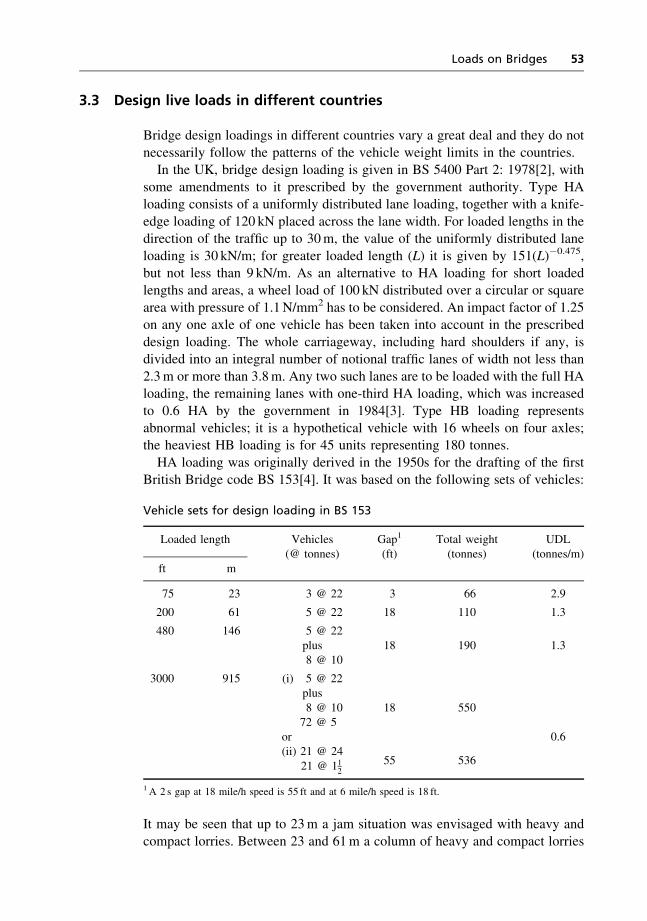
3.3 Design live loads in different countries

Bridge design loadings in different countries vary a great deal and they do not

necessarily follow the patterns of the vehicle weight limits in the countries.In the UK, bridge design loading is given in BS 5400 Part 2: 1978[2], with

some amendments to it prescribed by the government authority. Type HAloading consists of a uniformly distributed lane loading, together with a knife-

edge loading of 120 kN placed across the lane width. For loaded lengths in thedirection of the traffic up to 30m, the value of the uniformly distributed lane

loading is 30 kN/m; for greater loaded length (L) it is given by 151(L)�0.475,but not less than 9 kN/m. As an alternative to HA loading for short loadedlengths and areas, a wheel load of 100 kN distributed over a circular or square

area with pressure of 1.1N/mm2 has to be considered. An impact factor of 1.25on any one axle of one vehicle has been taken into account in the prescribed

design loading. The whole carriageway, including hard shoulders if any, isdivided into an integral number of notional traffic lanes of width not less than

2.3m or more than 3.8m. Any two such lanes are to be loaded with the full HAloading, the remaining lanes with one-third HA loading, which was increased

to 0.6 HA by the government in 1984[3]. Type HB loading representsabnormal vehicles; it is a hypothetical vehicle with 16 wheels on four axles;the heaviest HB loading is for 45 units representing 180 tonnes.

HA loading was originally derived in the 1950s for the drafting of the firstBritish Bridge code BS 153[4]. It was based on the following sets of vehicles:

It may be seen that up to 23m a jam situation was envisaged with heavy and

compact lorries. Between 23 and 61m a column of heavy and compact lorries

Vehicle sets for design loading in BS 153

Loaded length Vehicles(@ tonnes)

Gap1

(ft)Total weight(tonnes)

UDL(tonnes/m)

ft m

75 23 3 @ 22 3 66 2.9

200 61 5 @ 22 18 110 1.3

480 146 5 @ 22plus 18 190 1.38 @ 10

3000 915 (i) 5 @ 22plus8 @ 10 18 55072 @ 5

or 0.6(ii) 21 @ 24

55 53621 @ 112

1A 2 s gap at 18 mile/h speed is 55 ft and at 6 mile/h speed is 18 ft.

Loads on Bridges 53

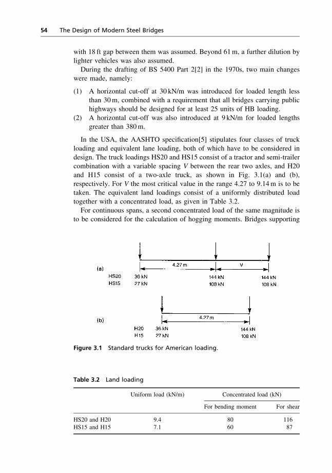
with 18 ft gap between them was assumed. Beyond 61m, a further dilution by

lighter vehicles was also assumed.During the drafting of BS 5400 Part 2[2] in the 1970s, two main changes

were made, namely:

(1) A horizontal cut-off at 30 kN/m was introduced for loaded length lessthan 30m, combined with a requirement that all bridges carrying public

highways should be designed for at least 25 units of HB loading.(2) A horizontal cut-off was also introduced at 9 kN/m for loaded lengths

greater than 380m.

In the USA, the AASHTO specification[5] stipulates four classes of truck

loading and equivalent lane loading, both of which have to be considered indesign. The truck loadings HS20 and HS15 consist of a tractor and semi-trailer

combination with a variable spacing V between the rear two axles, and H20and H15 consist of a two-axle truck, as shown in Fig. 3.1(a) and (b),

respectively. For V the most critical value in the range 4.27 to 9.14m is to betaken. The equivalent land loadings consist of a uniformly distributed load

together with a concentrated load, as given in Table 3.2.For continuous spans, a second concentrated load of the same magnitude is

to be considered for the calculation of hogging moments. Bridges supporting

Figure 3.1 Standard trucks for American loading.

Table 3.2 Land loading

Uniform load (kN/m) Concentrated load (kN)

For bending moment For shear

HS20 and H20 9.4 80 116HS15 and H15 7.1 60 87


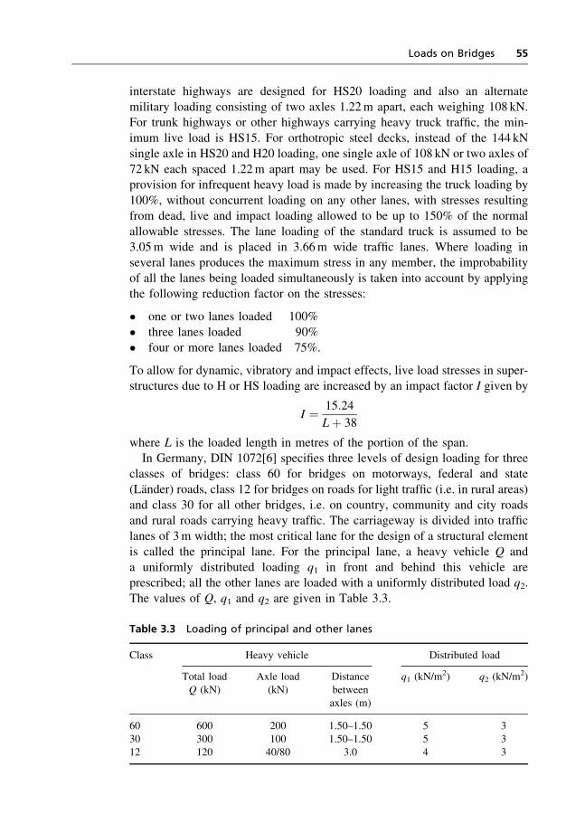
interstate highways are designed for HS20 loading and also an alternate

military loading consisting of two axles 1.22m apart, each weighing 108 kN.For trunk highways or other highways carrying heavy truck traffic, the min-

imum live load is HS15. For orthotropic steel decks, instead of the 144 kNsingle axle in HS20 and H20 loading, one single axle of 108 kN or two axles of

72 kN each spaced 1.22m apart may be used. For HS15 and H15 loading, aprovision for infrequent heavy load is made by increasing the truck loading by

100%, without concurrent loading on any other lanes, with stresses resultingfrom dead, live and impact loading allowed to be up to 150% of the normal

allowable stresses. The lane loading of the standard truck is assumed to be3.05m wide and is placed in 3.66m wide traffic lanes. Where loading inseveral lanes produces the maximum stress in any member, the improbability

of all the lanes being loaded simultaneously is taken into account by applyingthe following reduction factor on the stresses:

� one or two lanes loaded 100%

� three lanes loaded 90%� four or more lanes loaded 75%.

To allow for dynamic, vibratory and impact effects, live load stresses in super-structures due to H or HS loading are increased by an impact factor I given by

I ¼ 15:24

Lþ 38

where L is the loaded length in metres of the portion of the span.In Germany, DIN 1072[6] specifies three levels of design loading for three

classes of bridges: class 60 for bridges on motorways, federal and state(Lander) roads, class 12 for bridges on roads for light traffic (i.e. in rural areas)

and class 30 for all other bridges, i.e. on country, community and city roadsand rural roads carrying heavy traffic. The carriageway is divided into traffic

lanes of 3m width; the most critical lane for the design of a structural elementis called the principal lane. For the principal lane, a heavy vehicle Q and

a uniformly distributed loading q1 in front and behind this vehicle areprescribed; all the other lanes are loaded with a uniformly distributed load q2.The values of Q, q1 and q2 are given in Table 3.3.

Table 3.3 Loading of principal and other lanes

Class Heavy vehicle Distributed load

Total loadQ (kN)

Axle load(kN)

Distancebetweenaxles (m)

q1 (kN/m2) q2 (kN/m

2)

60 600 200 1.50–1.50 5 330 300 100 1.50–1.50 5 312 120 40/80 3.0 4 3

Loads on Bridges 55

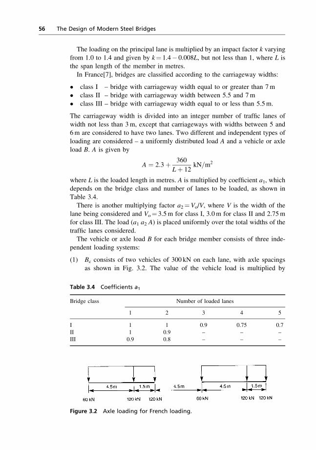
The loading on the principal lane is multiplied by an impact factor k varying

from 1.0 to 1.4 and given by k¼ 1.4� 0.008L, but not less than 1, where L isthe span length of the member in metres.

In France[7], bridges are classified according to the carriageway widths:

� class I – bridge with carriageway width equal to or greater than 7m� class II – bridge with carriageway width between 5.5 and 7m

� class III – bridge with carriageway width equal to or less than 5.5m.

The carriageway width is divided into an integer number of traffic lanes of

width not less than 3m, except that carriageways with widths between 5 and6m are considered to have two lanes. Two different and independent types of

loading are considered – a uniformly distributed load A and a vehicle or axleload B. A is given by

A ¼ 2:3þ 360

Lþ 12kN=m2

where L is the loaded length in metres. A is multiplied by coefficient a1, whichdepends on the bridge class and number of lanes to be loaded, as shown in

Table 3.4.There is another multiplying factor a2¼Vo/V, where V is the width of the

lane being considered and Vo¼ 3.5m for class I, 3.0m for class II and 2.75mfor class III. The load (a1 a2 A) is placed uniformly over the total widths of the

traffic lanes considered.The vehicle or axle load B for each bridge member consists of three inde-

pendent loading systems:

(1) Bc consists of two vehicles of 300 kN on each lane, with axle spacings

as shown in Fig. 3.2. The value of the vehicle load is multiplied by

Table 3.4 Coefficients a1

Bridge class Number of loaded lanes

1 2 3 4 5

I 1 1 0.9 0.75 0.7II 1 0.9 – – –III 0.9 0.8 – – –

Figure 3.2 Axle loading for French loading.


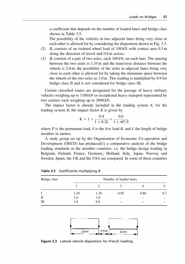
a coefficient that depends on the number of loaded lanes and bridge class

shown in Table 3.5.The possibility of the vehicles in two adjacent lanes being very close to

each other is allowed for by considering the disposition shown in Fig. 3.3.(2) Br consists of an isolated wheel load of 100 kN with contact area 0.3m

along the direction of travel and 0.6m across.(3) Bt consists of a pair of two axles, each 160 kN, on each lane. The spacing

between the two axles is 1.35m and the transverse distance between thewheels is 2.0m; the possibility of the axles in adjacent lanes being very

close to each other is allowed for by taking the minimum space betweenthe wheels of the two axles as 1.0m. This loading is multiplied by 0.9 forbridge class II and is not considered for bridge class III.

Certain classified routes are designated for the passage of heavy military

vehicles weighing up to 1100 kN or exceptional heavy transport represented bytwo carriers each weighing up to 2000 kN.

The impact factor is already included in the loading system A; for theloading system B, the impact factor K is given by

K ¼ 1þ 0:4

1þ 0:2Lþ 0:6

1þ 4P=S

where P is the permanent load, S is the live load B, and L the length of bridge

member in metres.A study group set up by the Organisation of Economic Co-operation and

Development (OECD) has produced[1] a comparative analysis of the bridgeloading standards in the member countries, i.e. the bridge design loading in

Belgium, Finland, France, Germany, Holland, Italy, Japan, Norway andSweden, Spain, the UK and the USA are compared. In some of these countries

Figure 3.3 Lateral vehicle disposition for French loading.

Table 3.5 Coefficients multiplying B

Bridge class Number of loaded lanes

1 2 3 4 5

I 1.20 1.20 0.95 0.80 0.7II 1.0 1.0 – – –III 1.0 0.8 – – –

Loads on Bridges 57

all bridges on public roads are designed for the same loading, whereas in the

other countries, the design loading depends on the type of route. Most codesprescribe the simultaneous action of a single concentrated or truck loading, and

a uniformly distributed load. Some codes consider the effect of a heavier axleor wheel load. The impact effect is already included in the design loads in

some codes, but in the other codes the design loading has to be increased bya factor which generally decreases with the length of the member. The

intensity of loading decreases with the increase in the loaded length in most ofthe codes. Most codes also allow a reduction when several traffic lanes have to

be loaded.This study also included a valuable numerical exercise of calculating the total

bending moments caused by the live loads of the various codes on a simply

supported bridge. Separate calculations were made for the bridge carrying two,three and four traffic lanes and spanning 10–100m. The total load on the whole

bridge was considered for this comparison, as if the bridge was supported byone single beam. The impact factor and the reduction due to multiple land

loading were taken into account; any difference between the various codes onthe allowable stress levels was also allowed for by multiplying the bending

moment by a ratio:

yield stress of steel specified in the national material specification

allowable stress of steel in the bridge design code

The bending moment M thus obtained was converted into an equivalent

uniformly distributed load qeq in kN/m, given by 8M/L2. These qeq valuesindicate the structural strength of bridges built according to the loading speci-fications of the various countries. Figures 3.4(a) and (b) show these qeq values

for bridges with two and four lanes in the carriageway, respectively. Very widedifferences between different countries are evident, the AASHTO loading

being by far the lightest for spans over 25m.

3.4 Recent developments in bridge loading

In recent years it has been found in several countries that the standard loadingdoes not satisfactorily reflect the effect of a long queue of vehicles in a traffic

jam situation, particularly for long loaded lengths of, say, over 40m. In theUSA, proposals[8] were made for a new loading standard which will consist of

a uniformly distributed load U and a concentrated load P for each lane, bothof which depend on the length of the bridge to be loaded for the worst effect.U depends also on the percentage of heavy goods vehicles in the traffic.

Table 3.6 gives typical values. No allowance for impact needs to be added, asthe loading represents a static jam situation. In multiple lanes, a second

lane shall have 70% of the basic lane load and all other lanes shall each have40%.


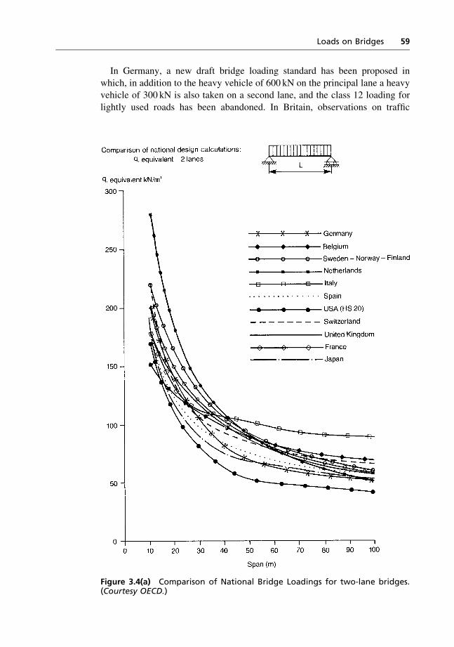
In Germany, a new draft bridge loading standard has been proposed in

which, in addition to the heavy vehicle of 600 kN on the principal lane a heavyvehicle of 300 kN is also taken on a second lane, and the class 12 loading for

lightly used roads has been abandoned. In Britain, observations on traffic

Figure 3.4(a) Comparison of National Bridge Loadings for two-lane bridges.(Courtesy OECD.)

Loads on Bridges 59

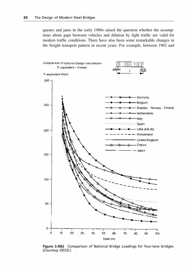
queues and jams in the early 1980s raised the question whether the assump-

tions about gaps between vehicles and dilution by light traffic are valid formodern traffic conditions. There have also been some remarkable changes in

the freight transport pattern in recent years. For example, between 1962 and

Figure 3.4(b) Comparison of National Bridge Loadings for four-lane bridges.(Courtesy OECD.)


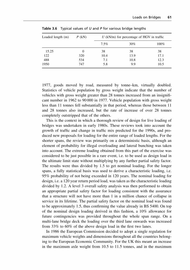
1977, goods moved by road, measured by tonne–km, virtually doubled.

Statistics of vehicle population by gross weight indicate that the number ofvehicles with gross weight greater than 28 tonnes increased from an insignifi-

cant number in 1962 to 90 000 in 1977. Vehicle population with gross weightless than 11 tonnes fell substantially in that period, whereas those between 11

and 28 tonnes also increased, but the rate of increase of over 28 tonnescompletely outstripped that of the others.

This is the context in which a thorough review of design for live loading ofbridges was undertaken in early 1980s. These reviews took into account thegrowth of traffic and change in traffic mix predicted for the 1990s, and pro-

duced new proposals for loading for the entire range of loaded lengths. For theshorter spans, the review was primarily on a deterministic basis, although an

element of probability for illegal overloading and lateral bunching was takeninto account. The extreme loading obtained from this part of the exercise was

considered to be just possible in a rare event, i.e. to be used as design load inthe ultimate limit state without multiplying by any further partial safety factor.

The results were thus divided by 1.5 to get nominal loading. For the longerspans, a fully statistical basis was used to derive a characteristic loading, i.e.

95% probability of not being exceeded in 120 years. The nominal loading fordesign, i.e. a 120 year return period load, was taken as the characteristic loadingdivided by 1.2. A level 3 overall safety analysis was then performed to obtain

an appropriate partial safety factor for loading consistent with the assurancethat a structure will not have more than 1 in a million chance of collapse in

service in its lifetime. The partial safety factor on the nominal load was foundto be approximately 1.5, thus confirming the value already in BS 5400. On top

of the nominal design loading derived in this fashion, a 10% allowance forfuture contingencies was provided throughout the whole span range. On a

multi-lane bridge deck the loading over the third lane onwards was increasedfrom 33% to 60% of the above design load in the first two lanes.In 1986 the European Commission decided to adopt a single regulation for

maximum vehicle weights and dimensions throughout all the countries belong-ing to the European Economic Community. For the UK this meant an increase

in the maximum axle weight from 10.5 to 11.5 tonnes, and in the maximum

Table 3.6 Typical values of U and P for various bridge lengths

Loaded length (m) P (kN) U (kN/m) for percentage of HGV in traffic

7.5% 30% 100%

15.25 0 38 38 38122 320 10.4 13.9 17.1488 534 7.1 10.8 12.31950 747 5.8 9.9 10.5

Loads on Bridges 61

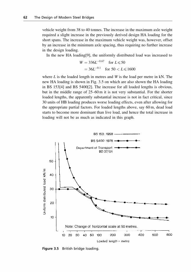
vehicle weight from 38 to 40 tonnes. The increase in the maximum axle weight

required a slight increase in the previously derived design HA loading for theshort spans. The increase in the maximum vehicle weight was, however, offset

by an increase in the minimum axle spacing, thus requiring no further increasein the design loading.

In the new HA loading[9], the uniformly distributed load was increased to

W ¼ 336L�0:67 for L450

¼ 36L�0:1 for 50 < L41600

where L is the loaded length in metres and W is the load per metre in kN. Thenew HA loading is shown in Fig. 3.5 on which are also shown the HA loading

in BS 153[4] and BS 5400[2]. The increase for all loaded lengths is obvious,but in the middle range of 25–60m it is not very substantial. For the shorter

loaded lengths, the apparently substantial increase is not in fact critical, since30 units of HB loading produces worse loading effects, even after allowing forthe appropriate partial factors. For loaded lengths above, say 60m, dead load

starts to become more dominant than live load, and hence the total increase inloading will not be as much as indicated in this graph.

Figure 3.5 British bridge loading.


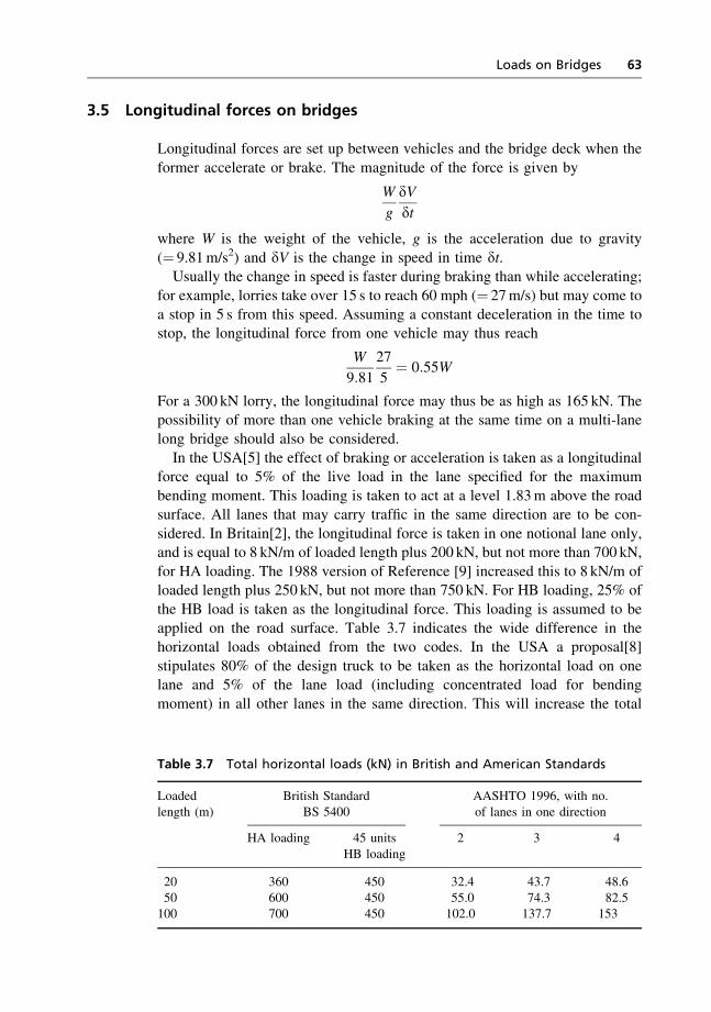
3.5 Longitudinal forces on bridges

Longitudinal forces are set up between vehicles and the bridge deck when the

former accelerate or brake. The magnitude of the force is given by

W

g

dVdt

where W is the weight of the vehicle, g is the acceleration due to gravity

(¼ 9.81m/s2) and dV is the change in speed in time dt.Usually the change in speed is faster during braking than while accelerating;

for example, lorries take over 15 s to reach 60 mph (¼ 27m/s) but may come toa stop in 5 s from this speed. Assuming a constant deceleration in the time tostop, the longitudinal force from one vehicle may thus reach

W

9:81

27

5¼ 0:55W

For a 300 kN lorry, the longitudinal force may thus be as high as 165 kN. Thepossibility of more than one vehicle braking at the same time on a multi-lanelong bridge should also be considered.

In the USA[5] the effect of braking or acceleration is taken as a longitudinalforce equal to 5% of the live load in the lane specified for the maximum

bending moment. This loading is taken to act at a level 1.83m above the roadsurface. All lanes that may carry traffic in the same direction are to be con-

sidered. In Britain[2], the longitudinal force is taken in one notional lane only,and is equal to 8 kN/m of loaded length plus 200 kN, but not more than 700 kN,

for HA loading. The 1988 version of Reference [9] increased this to 8 kN/m ofloaded length plus 250 kN, but not more than 750 kN. For HB loading, 25% of

the HB load is taken as the longitudinal force. This loading is assumed to beapplied on the road surface. Table 3.7 indicates the wide difference in thehorizontal loads obtained from the two codes. In the USA a proposal[8]

stipulates 80% of the design truck to be taken as the horizontal load on onelane and 5% of the lane load (including concentrated load for bending

moment) in all other lanes in the same direction. This will increase the total

Table 3.7 Total horizontal loads (kN) in British and American Standards

Loadedlength (m)

British StandardBS 5400

AASHTO 1996, with no.of lanes in one direction

HA loading 45 unitsHB loading

2 3 4

20 360 450 32.4 43.7 48.650 600 450 55.0 74.3 82.5100 700 450 102.0 137.7 153

Loads on Bridges 63

horizontal load very substantially, bringing the value for HS20 loading nearer

to the British value. The German code[10] specifies a horizontal load of 5% ofthe distributed loading q1 on the carriageway up to a loaded length of 200m

but not less than 0.3 times the design heavy vehicle Q (see Section 3.3); but inthe new proposals, this is being increased to 10% of the distributed loading q1on the carriageway up to 12m wide and 200m long, but not less than one-thirdof the design heavy vehicles Q in the main and second lanes.

3.6 Wind loading

Wind load on a bridge may act:

(1) horizontally, transverse to the direction of the span

(2) horizontally, along the direction of the span(3) vertically, upwards causing uplift.

Wind load is not generally significant for short-span bridges; for medium

spans, the design of the sub-structure may be affected by wind loading; thesuperstructure design is affected by wind only for long spans.

For bridges with high natural frequency of vibration, only the static loadingeffect of wind needs to be considered. The dynamic effect of wind, and theoscillation caused by it, is, however, very important for bridges with low

natural frequency.In the AASHTO code[5] the transverse wind load is specified as 3.6 kN/m2

for trusses and arches and 2.4 kN/m2 for girders and beams, to be applied to thetotal exposed area in elevation. The following minimum values are also

specified, corresponding to wind velocity of 161 km/h:

(1) 4.4 kN/m in the plane of the windward chord of a truss(2) 2.2 kN/m in the plane of the leeward chord of a truss

(3) 4.4 kN/m on girder spans.

All these values may be reduced if a lower velocity is appropriate to the

particular location. These values are appropriate to the bridge carrying no trafficload. When traffic is present, only 30% of the above load on the structure is

taken, plus a loading of 1.5 kN/m acting at 1.83m above the deck. For theeffect on sub-structures, forces in both transverse and longitudinal directions

are to be taken, their magnitudes depending on the angle of skew. For zeroskew angle, the transverse forces are as mentioned above and the longitudinal

forces are zero; the former decreases and the latter increases with increase inthe skew angle. The wind loading on the sub-structure itself is taken as1.92 kN/m2, corresponding to 161 km/h wind speed, and the wind force is

resolved into transverse and longitudinal components corresponding to theskew angle of the wind direction. When traffic is present, only 30% of the wind

loading on superstructure and substructure is considered along with the full


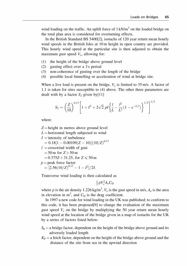
wind loading on the traffic. An uplift force of 1 kN/m2 on the loaded bridge on

the total plan area is considered for overturning effects.In the British Standard BS 5400[2], isotachs of 120 year return mean hourly

wind speeds in the British Isles at 10m height in open country are provided.This hourly wind speed at the particular site is then adjusted to obtain the

maximum gust speed Vc, allowing for:

(1) the height of the bridge above ground level

(2) gusting effect over a 3 s period(3) non-coherence of gusting over the length of the bridge

(4) possible local funnelling or acceleration of wind at bridge site.

When a live load is present on the bridge, Vc is limited to 35m/s. A factor of1.1 is taken for sites susceptible to (4) above. The other three parameters aredealt with by a factor S2 given by[11]

S2 ¼ Z

10

� �0:17

1þ I2 þ 2ffiffiffi2

ppI

l

L� l2

L2ð1� e�L=lÞ

� �1=2" #1=2

where

Z¼ height in metres above ground level

L¼ horizontal length subjected to windI ¼ intensity of turbulence

¼ 0:18½1� 0:00109ðZ � 10Þ�ð10=ZÞ0:17l ¼ crosswind width of gust

¼ 50m for Z> 50m¼ 0.375Zþ 31.25, for Z4 50m

p¼ peak force factor

¼ ½2:56ð10=ZÞ0:17 � 1� I2�=2I:Transverse wind loading is then calculated as

12 rV

2cAeCD

where r is the air density 1.226 kg/m3, Vc is the gust speed in m/s, Ae is the area

in elevation in m2, and CD is the drag coefficient.In 1997 a new code for wind loading in the UK was published; to conform to

this code, it has been proposed[9] to change the evaluation of the maximumgust speed Vc on the bridge by multiplying the 50 year return mean hourly

wind speed at the location of the bridge given in a map of isotachs for the UKby a series of factors listed below:

Sb¼ a bridge factor, dependent on the height of the bridge above ground and its

adversely loaded lengthKF¼ a fetch factor, dependent on the height of the bridge above ground and the

distance of the site from sea in the upwind direction

Loads on Bridges 65

Tg¼ a town reduction factor, dependent on the distance of the site from the

edge of any urban area in the upwind directionSh¼ a topography factor, which is generally 1.0, but should be taken as 1.1

when local funnelling or acceleration of wind can occurSp¼ a probability factor, to be taken as 1.05 for 120 year return period wind

loading and 1.0 for 50 year return periodSa¼ an altitude factor, to be taken as (1þ�/1000), where � is the height of

the bridge in metres above mean sea levelSd¼ a wind direction factor dependent on critical wind direction; it varies from

0.73 for north to northeast to 1.0 for westerly critical wind direction.

For plate or box girder types of bridges, the area in elevation includes a 2.5mhigh vertical surface above the bridge deck for wind loading on vehicles; anysolid parapet is also included, but wind loads on open parapets are calculated

separately. For truss bridges, wind loads are calculated separately for:

(1) windward and leeward girders

(2) windward and leeward parapets(3) area in elevation of the deck structure

(4) live load height 2.5m above deck.

Any screening offered by an adjacent component can be taken advantage of.

For plate and box girder types of bridges, the drag coefficient CD isdependent upon the ratio of the width b of the bridge to its maximum depth d

as seen in the bridge cross-section. The value of CD varies from 1.4 for a b/dratio of 4, to 1.0 for a b/d ratio equal to or greater than 12. For a very narrow

and deep bridge cross-section with a b/d ratio of 0.6, CD reaches a peak valueof 2.75. For truss girder bridges with flat-sided members, CD for the windward

truss is dependent upon the solidity ratio, i.e. the net area to the overall area ofthe truss in elevation; CD varies from 1.9 to 1.6 for solidity ratio 0.1 to 0.5. Fortrusses with round members, CD for the windward girder is 1.2 or 0.8

depending on whether gust speed� diameter < or 56m2/s. For the leewardtruss, this drag coefficient is multiplied by a shielding factor which depends on

both the solidity ratio defined above and the spacing ratio, i.e. the distancebetween the trusses divided by their depth. The shielding factor varies from 1.0

for the solidity ratio of 0.1 and any spacing ratio, to 0.45 for solidity ratio 0.5and spacing ratio 1, and to 0.7 for solidity ratio 0.5 and spacing ratio 6. The

drag coefficient for unshielded parts of the live load is taken as 1.45. Tables aregiven for CD for different shapes of parapets and bridge piers.

The longitudinal wind load on superstructures is taken as one-quarter of thetransverse wind load on plate or box girder bridges, one-half of the transversewind load on trusses, and also one-half of the transverse wind load on vehicles.

Upward or downward wind load is taken as

12rV

2cApCL


where r is the air density¼ 1.226 kg/m3, Vc is the gust speed in m/s, Ap is the

plan area in m2, and CL is the lift coefficient.For bridges with deck superelevation up to 1�, CL is 0.4 for b/d ratio up to 7

and 0.15 for b/d ratio greater than 16, with a linear variation in between; forsuperelevation between 1� and 5�, CL is 0.75.

A combination of full transverse and vertical loading due to wind is con-sidered, but full longitudinal loading is considered in combination with half the

transverse and vertical loading.The American bridge loading proposals[8] are similar to, but probably not as

detailed as, the British loading. The transverse wind loading on the full area inelevation is stipulated as

Z0:2V230CD

600lb=ft2

where Z is the height in feet of the bridge deck surface above ground or water

level but not less than 30 ft, V30 is the 100 year return fastest mile wind speedin miles per hour at the 30 ft height and can be obtained from the map of

isotachs or preferably from local wind data, and CD is the drag coefficient andis specified as 1.5 for plate or box girder bridges and 2.3 for truss bridges

unless a lower value is justified by wind tunnel tests. When a live load ispresent on the bridge, a vertical surface of 10 ft height, less the area shielded bysolid parapets, is included in the total area in elevation, CD is specified as 1.2

on this part, and V30 is limited to 55 mile/h. The vertical wind load on the planarea of the bridge is stipulated as

Z0:2V230CL

600lb=ft2

where CL is the lift coefficient specified as 1.0.The above two proposed formulae for wind load are based on the following

assumptions:

(1) The maximum gust speed is approximately 1.6 times the mean hourlywind speed, but because of the incoherence of gusts along the wholelength of the bridge the gust speed is reduced to 1.41 times the mean

hourly speed.(2) At heights above 30 ft the gust speed is assumed to increase according to

the 1/10th power of height.(3) The mean hourly wind speed is 0.8 times V30, the fastest mile wind speed

at 30 ft, in which form the wind speed is recorded in the USA.(4) The maximum gust speed, unlike the mean hourly speed, is relatively

insensitive to terrain condition.

At 30 ft height and V30¼ 100 mile/h, the new formulae give very similar

wind loads to the current AASHTO values, but for other heights and locationsthe new values will obviously be different. At Z¼ 30 ft and V30¼ 80 mile/h,

Loads on Bridges 67

the horizontal wind pressure given by the new loading is 21 lb/ft2, which can be

compared with the values of 23 and 19.5 lb/ft2 given by the British Standard formean hourly wind speed of 64 mile/h, 10m height and bridge lengths 60m and

200m, respectively. The proposed American drag coefficients of 1.5 and 2.3for solid and truss girders may be compared with the British values of 1.4 to

1.0 for solid girders with b/d ratios ranging from 4 to 12, and 1.6 on thewindward truss and 0.7 on the leeward truss with flat-sided members, with a

solidity ratio of 0.5 and a shielding factor of 0.5. The lift coefficient of 1.0 forvertical wind load in the American proposals can be compared with the British

value of 0.75 for superelevation between 1 and 5 degrees. With traffic presenton the bridge the American proposal specifies V30¼ 55 mile/h, which isequivalent to a gust speed of 1.41� 0.8� 55¼ 62 mile/h or 27.6m/s, but with

the wind load dependent upon the height of the bridge deck above ground orwater level; this may be compared with the gust speed of 35m/s for all heights

stipulated in the British code.In the German code[6], wind load is specified as 2.5 kN/m2 without traffic,

and 1.25 kN/m2 with traffic, to be applied to the area in projected elevation ofthe bridge. The traffic profile is taken as a 2m high vertical surface above the

bridge deck. The German loading[10] retains the above wind loading forbridges with superstructure 50 to 100m above ground level, but makesreductions for:

(1) superstructures at lower height

(2) superstructures with noise barriers, in the load case without traffic.

It also increases the height of the traffic profile to 3.5m.

3.7 Thermal forces

If the free expansion or contraction of a structure due to changes in tempera-ture is restrained by its form of construction (e.g. portal frame, arch) or by

bearings or piers, then stresses are set up inside the structure. Secondly, dif-ferences in temperature through the depth of the superstructure set up stresses

if the structure is not free to deform. A differential temperature pattern in thedepth of the structure represented by a single continuous straight line from the

top to the bottom surface does not cause stresses in a statically determinatestructure, e.g. simply supported or balanced cantilever spans, but will cause

stresses in a continuous structure due to the vertical restraints provided by thepiers. Normally differential temperature is not represented by a single con-tinuous line from the top to the bottom surface, and hence causes stresses even

in simple spans.In the British Standard BS 5400[2], maps of isotherms provide the extremes

of shade air temperatures at sea level in different parts of the British Isles. Forheights above sea level these temperatures are reduced by 0.5�C and 1.0�C for


minimum and maximum temperatures, respectively, for every 100m height.

Local peculiarities like frost pockets, sheltered areas, urban or coastal sitesshould also be taken into account. The minimum temperature in the bridge

structure is usually lower than the minimum shade air temperature by 2�C to4�C for bridges with steel orthotropic decks and higher by 1�C to 8�C for

bridges with concrete decks; the maximum bridge temperature is higher thanthe maximum shade air temperature by between 9�C and 20�C for bridges with

steel decks and by up to 11�C for bridges with concrete decks. The differencebetween the bridge and the shade air temperatures depend upon the latter and

also on the type and depth of surfacing provided on the bridge deck; data forthese differences are tabulated in the British code[2]. Within this range of thebridge temperatures, the variation with respect to the particular datum tem-

perature at which restraint was imposed on the bridge during its constructiondetermines the magnitudes of thermal stresses.

In the AASHTO code[5], a range of bridge temperatures of �18�C toþ49�C is specified for a moderate climate and �34�C to þ49�C for a cold

climate.The differential temperature pattern given in the British code[2] is based on

extensive measurements on bridges in the British Isles and deals with varioustypes of bridge decks and deck surfacings. For the common case of a steel plateor box or truss girder construction with (1) a 230mm thick concrete slab and

100mm of deck surfacing and (2) a steel orthotropic deck with 40mm ofsurfacing, the temperature differential with the road surface in the hot and cold

conditions are as shown in Fig. 3.6.The AASHTO code[5] does not specify any temperature differential, but the

proposals[8] stipulate the pattern shown in Fig. 3.7.In the German code[6], the temperature at the time of construction is

assumed to be þ10�C and a variation of �35�C from the construction tem-perature is to be considered; within this range, a differential temperature of

15�C, linearly varying between different parts of the bridges structure, is alsoto be considered, for example between top and bottom flanges, between cablesand stiffening girders, between webs of box girders.

In composite structures, i.e. steel structures with concrete slabs, a temperatureincrease or decrease in the top surface of the slab of 20�C and at the bottom edge

of the steel girder of 35�C, from the construction temperature of þ10�C, isspecified. In the German proposals[10] clarifications have been made that

differential temperature need only be considered in the vertical plane and themagnitudes have been proposed to be reduced to 10�C with the deck hot, 5�Cwith the deck cold for a steel deck bridge and 7�C with the deck cold for acomposite bridge with a concrete deck. With traffic load on the bridge, eitherdifferential temperature or the traffic loadmay be reduced to 70%.A temperature

difference of �15�C between different members of a bridge that are generallyunconnected to each other should also be considered, for example between the

beam and arch, cables and deck structure, upper and lower chords of trusses.

Loads on Bridges 69

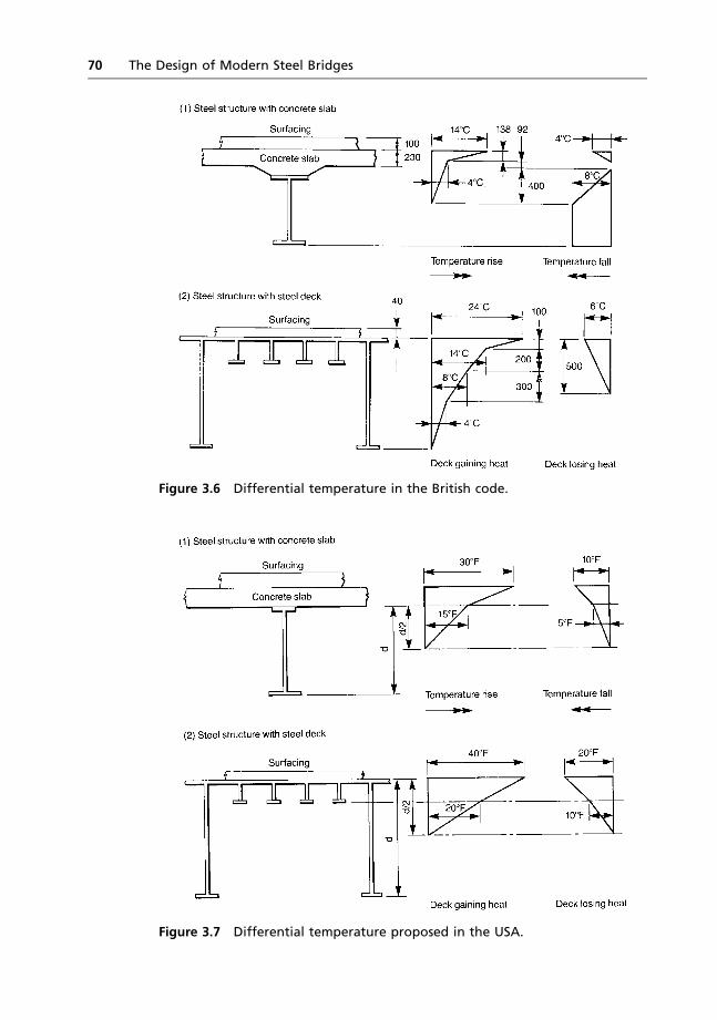
Figure 3.7 Differential temperature proposed in the USA.

Figure 3.6 Differential temperature in the British code.


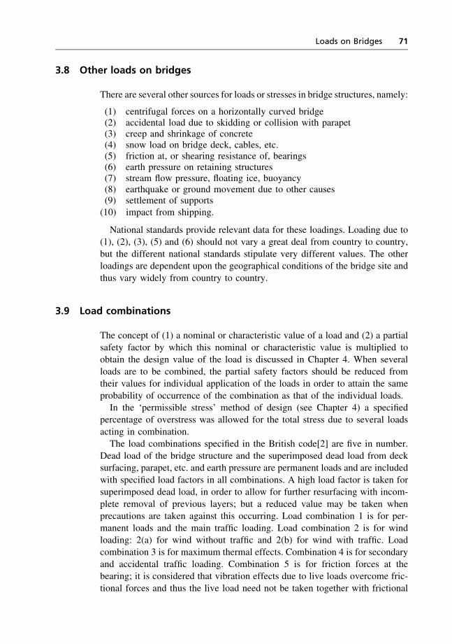
3.8 Other loads on bridges

There are several other sources for loads or stresses in bridge structures, namely:

(1) centrifugal forces on a horizontally curved bridge(2) accidental load due to skidding or collision with parapet(3) creep and shrinkage of concrete(4) snow load on bridge deck, cables, etc.(5) friction at, or shearing resistance of, bearings(6) earth pressure on retaining structures(7) stream flow pressure, floating ice, buoyancy(8) earthquake or ground movement due to other causes(9) settlement of supports(10) impact from shipping.

National standards provide relevant data for these loadings. Loading due to(1), (2), (3), (5) and (6) should not vary a great deal from country to country,

but the different national standards stipulate very different values. The otherloadings are dependent upon the geographical conditions of the bridge site and

thus vary widely from country to country.

3.9 Load combinations

The concept of (1) a nominal or characteristic value of a load and (2) a partial

safety factor by which this nominal or characteristic value is multiplied toobtain the design value of the load is discussed in Chapter 4. When several

loads are to be combined, the partial safety factors should be reduced fromtheir values for individual application of the loads in order to attain the same

probability of occurrence of the combination as that of the individual loads.In the ‘permissible stress’ method of design (see Chapter 4) a specified

percentage of overstress was allowed for the total stress due to several loads

acting in combination.The load combinations specified in the British code[2] are five in number.

Dead load of the bridge structure and the superimposed dead load from decksurfacing, parapet, etc. and earth pressure are permanent loads and are included

with specified load factors in all combinations. A high load factor is taken forsuperimposed dead load, in order to allow for further resurfacing with incom-

plete removal of previous layers; but a reduced value may be taken whenprecautions are taken against this occurring. Load combination 1 is for per-

manent loads and the main traffic loading. Load combination 2 is for windloading: 2(a) for wind without traffic and 2(b) for wind with traffic. Loadcombination 3 is for maximum thermal effects. Combination 4 is for secondary

and accidental traffic loading. Combination 5 is for friction forces at thebearing; it is considered that vibration effects due to live loads overcome fric-

tional forces and thus the live load need not be taken together with frictional

Loads on Bridges 71

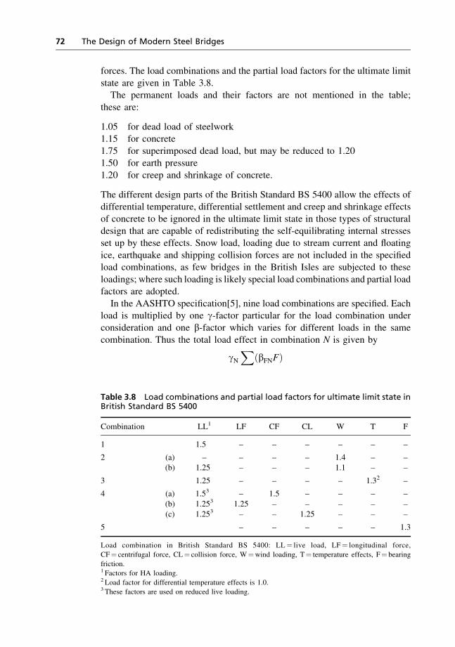
forces. The load combinations and the partial load factors for the ultimate limit

state are given in Table 3.8.The permanent loads and their factors are not mentioned in the table;

these are:

1.05 for dead load of steelwork1.15 for concrete

1.75 for superimposed dead load, but may be reduced to 1.201.50 for earth pressure

1.20 for creep and shrinkage of concrete.

The different design parts of the British Standard BS 5400 allow the effects ofdifferential temperature, differential settlement and creep and shrinkage effects

of concrete to be ignored in the ultimate limit state in those types of structuraldesign that are capable of redistributing the self-equilibrating internal stressesset up by these effects. Snow load, loading due to stream current and floating

ice, earthquake and shipping collision forces are not included in the specifiedload combinations, as few bridges in the British Isles are subjected to these

loadings; where such loading is likely special load combinations and partial loadfactors are adopted.

In the AASHTO specification[5], nine load combinations are specified. Eachload is multiplied by one g-factor particular for the load combination under

consideration and one b-factor which varies for different loads in the samecombination. Thus the total load effect in combination N is given by

gNX

ðbFNFÞ

Table 3.8 Load combinations and partial load factors for ultimate limit state inBritish Standard BS 5400

Combination LL1 LF CF CL W T F

1 1.5 – – – – – –

2 (a) – – – – 1.4 – –(b) 1.25 – – – 1.1 – –

3 1.25 – – – – 1.32 –

4 (a) 1.53 – 1.5 – – – –(b) 1.253 1.25 – – – – –(c) 1.253 – – 1.25 – – –

5 – – – – – 1.3

Load combination in British Standard BS 5400: LL¼ live load, LF¼ longitudinal force,

CF¼ centrifugal force, CL¼ collision force, W¼wind loading, T¼ temperature effects, F¼ bearing

friction.1 Factors for HA loading.2 Load factor for differential temperature effects is 1.0.3 These factors are used on reduced live loading.


where F represents the load due to dead load, live load, wind load, etc. and bFNis the factor on the particular load for the particular combination N. Dead load,earth pressure, buoyancy and stream flow pressure are considered permanent

forces and are included in all the load combinations with the followingb-factors:

� dead load ¼ 1.0 except that a smaller factor of 0.75 is taken for

minimum load and maximum moment in columns� earth pressure ¼ 1.3 for maximum lateral pressure

¼ 0.5 for minimum lateral pressure

¼ 1.0 for vertical earth pressure� buoyancy ¼ 1.0

� stream pressure¼ 1.0.

Combination 1 is the main combination with live load, combination 2 is forwind load on unloaded bridges and combination 3 is for wind load on bridges

carrying traffic. Combination 4 is for temperature and shrinkage effects withlive load and combination 5 is for temperature and shrinkage effects with high

wind and no live load. Combination 6 is an omnibus combination with all theabove loads, but with a reduced g-factor to represent the reduced likelihood ofall the forces acting with their peak values. Combinations 4, 5 and 6 are

dominated by the forces due to shrinkage and thermal effects and are thuscritical for those structures that are restrained against longitudinal expansion or

contraction, i.e. arches and portal frames. Combination 7 is for earthquakeforces, to be taken in conjunction with only the permanent loads. Combinations

8 and 9 are for ice pressure on substructures, to be combined with live loadsonly in the former combination, and with wind load only in the latter.

In comparing the g and b factors in the AASHTO specification with thepartial load factors in BS 5400, it has to be remembered that in the latter codetwo other partial factors are to be considered. These are:

(1) gf3 – this takes account of inaccuracies in the assessment of load effects,

or in the calculation model or in the overall dimensions, and is taken as1.1 in the ultimate limit state

(2) gm – this is the partial factor for material strength and is generally 1.05for structural steel.

References

1. Evaluation of Load Carrying Capacity of Bridges: 1979. Organisation for

Economic Co-operation and Development, Paris.

2. BS 5400: Part 2: 1978. Steel, Concrete and Composite Bridges: Specification for

Loads: British Standards Institution, London.

3. Departmental Standard BD 23/84: Loads for Highway and Foot/Cycle Track

Bridges. Department of Transport, London.

Loads on Bridges 73

4. British Standard 153: 1958. Specification for Steel Girder Bridges. British Standards

Institution, London.

5. AASHTO Standard Specifications for Highway Bridges: 1996. The American

Association of State Highway and Transportation Officials, Washington.

6. Deutsche Normen DIN 1072: 1967. Road and Footbridges: Design Loads. Berlin.

7. Cahier des prescriptions communes applicables aux marches de travaux publis

relevant des services de l’equipement: 1973. Ministere de l’Equipement et du

Logement – Ministere des Transports, Paris.

8. Recommended design loads for bridges. Committee on Loads and Forces on

Bridges of the Committee on Bridges of the Structural Division. Journal of the

Structural Division, Proceedings of the American Society of Civil Engineers.

December 1981.

9. Departmental Standard BD 37/01: Loads for Highway Bridges: Department of

Transport, London.

10. Deutsche Normen. Draft DIN 1072: August 1983: Road and Footbridges: Design

Loads. Berlin.

11. Hay J. S.: 1974. Estimation of wind speed and air temperature for the design of

bridges. Laboratory Report LR 599, Transport and Road Research Laboratory,

England.


Chapter 4

Aims of Design

4.1 Limit state principle

The aim of design is that the structure should:

(1) sustain all loads and deformations liable to occur during its construction,

use and also foreseeable misuse or accident(2) perform adequately in normal use

(3) have adequate durability.

When a structure or any of its components infringes one of its criteria forperformance or use, it is said to have exceeded a limit state. For most structuresthe limit states can be placed in two categories:

(1) the ultimate limit states which are related to a collapse of the whole or

a substantial part of the structure(2) the serviceability limit states which are related to disruption of the normal

use of the structure.

Ultimate limit states should have a very low probability of occurrence, sincethey may cause loss of life, amenity and investment. The common ultimate

limit states are:

(1) loss of static equilibrium of a part or the whole of the structure consideredas a rigid body (e.g. overturning, uplift, sliding)

(2) loss of load-bearing capacity of a member due to its material strengthbeing exceeded, or due to buckling, or a combination of these two phenom-

ena, or fatigue(3) overall instability, leading to very large deformation or collapse, caused

by, for example, aerodynamic or elastic critical behaviour or transforma-

tion into a mechanism.

The serviceability limit states depend on the function of the structures; forbridges they correspond to:

(1) excessive deformation of the structure, or any of its parts, affecting the

appearance, functional use or drainage, or causing damage to non-structural components like deck joints, surfacing, etc.

75

(2) excessive local damage like cracking, splitting, spalling, yielding or slip,

affecting appearance, use or durability of the structure(3) excessive vibration causing discomfort to pedestrians or drivers.

4.2 Permissible stress method

In the modern generation of structural design codes, the specific requirementsfor the relevant limit states are stated explicitly. In the past, however, the codes

did not identify the various limit states separately; they were like a cookingrecipe which produced the desired end product, but the ingredients of which

were not specifically chosen for particular objectives.The process of structural design is not an exact science, nor are the data on

which a design can be based accurate. There are uncertainties in the loading, in

the material properties, in the engineering analysis and in the constructionprocess. In the past, design codes allowed for these uncertainties by specifying

a permissible stress for the most adverse combination of working loads. Thepermissible stress was obtained by applying a factor of safety on the stress

observed or calculated to occur at failure. The failure stress was generallytaken as the yield stress and the working loads were specified as those loads

that could be expected to act on the structure several times in its design life.In this permissible stress or working load method a structural analysis was

made to evaluate the working stresses at the specified combination of working

loads, which were then checked against the specified permissible stress. ThusXworking stress4permissible stress

i.e.4failure stress

safety factor

The main advantage of this method is simplicity. Because stresses, andhence deformations/deflections, were kept low under working loads, non-

linearity of material and/or structural behaviour could be neglected and workingstresses were calculated from linear elastic theories. Stresses from variousloads could thus be added together. The disadvantages of this method are:

(1) One global factor of safety cannot deal with the different variabilities of

different loads; for example, variations of dead load from the calculatedworking value is usually small compared with the variation of extreme

wind or vehicle loads from their working values. This is particularlyserious when two loads of different variabilities counteract each other;

the safety factor used in this method may give a very false impressionof the danger that can be caused by a modest increase in one of the loads.

(2) The analysis of the structure under working loads may not provide arealistic assessment of the behaviour of the structure at failure. If the


critical components of the structure possess sufficient ductility,

redistribution of load takes place after some of these components reachthe limit of their linear behaviour, thus mobilising the strength of the less

critical components. Formation of successive plastic hinges in a con-tinuous beam or frame is one example. Here the safety factor in the

working stress method may represent a too pessimistic ratio of the realultimate strength of the structure to the working load. Conversely, in

some structures or structural components, stresses increase faster than theloads and thus the real ultimate load is less than the working load times

the safety factor.

Structures designed by the permissible stress/working load methods used to

have moderate stresses in service conditions and thus the serviceabilityrequirements like deflections, cracking, yielding, slip and vibrations were not

generally critical and hence did not require checking. However, post-wardevelopments of materials of higher strength, welding and pre-stressing have

necessitated explicit serviceability requirements in various design codes, oftenin the form of empirical rules.

4.3 Limit state codes

In the modern limit state design codes, a calculation model is established for

each limit state to verify that the probability of its non-exceedance is equal toor higher than a pre-defined target reliability of the structure. This model

incorporates:

(1) all the possible modes in which the particular limit state may be exceeded(2) the uncertainties of all the variable parameters involved in the model,

and the uncertainty or approximation of the model itself(3) the target reliability.

The latter is often a compromise between the initial cost of the structure andthe consequences of the exceedance of the limit state, and is guided by past

experiences of design and performance of similar types of structures. Thevariable parameters are commonly the ‘actions’ (i.e. forces and constrained

deformations), the properties of materials, the geometrical parameters of thestructure, and the inaccuracy of the model itself. In the mathematical model

their variabilities can be treated by different levels of approximation. These are:

(1) Level III – this is the most complex method; the full probability distri-bution of all the design variables is integrated numerically by multidimensionalconvolution integrals to compute the exact probability of failure of the

structural system in all the possible modes. Because of its inherent numericaldifficulties it is not suitable for design purposes except for very special

structures.

Aims of Design 77

(2) Level II – in this method some idealisations are introduced into the

probability analysis to reduce the numerical difficulties; thus, for each mode offailure, a failure boundary is defined by structural theories in the space of the

variable parameters, from the probability distribution of the variables achecking point on the failure boundary is identified where failure is most likely

to occur, and by linearising the failure boundary at the design point anapproximate reliability of the structure is estimated.

(3) Level I – this is a semi-probablistic method in which appropriate levels ofreliability are achieved for each structural element by the application of a

number of partial safety factors to a pre-defined set of characteristic values ofthe variables. The characteristic value of each variable has a pre-defined low

probability of occurrence and is determined, wherever possible, from the meanvalue, the standard deviation and the distribution type of the variable obtained

by tests or measurement. When statistical data are not available, nominalvalues based on past practice are used. The partial safety factors may be

determined by a Level II (or III) method for the required degree of safety. Thusthe Level I method can be made identical to Level II (or III) if the partial safety

factors are expressed as continuous functions of the means, standard deviationsand distribution types of the variables. However, most structural codes draftedin Level I format prescribe discrete values of the safety factors instead of

continuous functions, to be applied to a rationalised, i.e. reduced, number ofdesign variables.

The idea that the statistical variation in a parameter should be considered in

structural design is not new. For example, the design wind speeds are deter-mined from the distribution of the annual extreme mean hourly speeds in the

British codes and of the annual extreme fastest mile speeds in North America.The acceptance criteria for the concrete mix are designed to ensure that theprobability of producing concrete with a cube strength less than the specified

characteristic value is less than a pre-defined target, which is 5% in the UK and10% in the USA. Probability based limit state codes recognise that, in the

presence of uncertainties, absolute reliability cannot be achieved, but theprobability of exceeding a limit state can be ensured to be acceptably low.

In between the permissible stress codes and the limit state codes there havebeen several intermediate developments. For example, the load and resistance

factor designs developed in the USA[1–3] use factored loads and factoredresistances, with different factors for different loads, reflecting their different

degrees of variability. ThusXðnominal loads� load factorÞ

4resistance

resistance factor

This method does not deal with all the limit states, and the factors are based onpast experience, intuition and perception regarding the uncertainties involved.


But this is an attempt to achieve uniform safety over the range of the likely

loads.The limit state codes developed in the UK, namely CP 110[4] and BS

5400[5], prescribe all the limit states that should be considered, but the partialsafety factors were again based on experience, intuition and judgement; only

in the case of the design code for steel bridges in BS 5400 were the resist-ance factors for the main ultimate limit states determined by a Level II

analysis[6].

4.4 The derivation of partial safety factors

In the concept of probability based design, a limit state is idealised as a

function

gðx1, x2, . . . , xnÞ ¼ 0

where the xi are independent variable parameters like actions, materialstrength, dimensions, etc.; the limit state is exceeded when g< 0. ProbabilityPf that the limit state is exceeded is then calculated from

Pf ¼ð. . .

ðfxðx1, x2, . . . , xnÞ dx1, dx2 . . . dxn

in which fx is the joint probability density function for x1, x2, . . . , xn, and theintegration is performed over the entire space when g< 0.

If a limit state function can be expressed in terms of just two independentvariables, i.e. a resistance variable R (e.g. the bending capacity of a beam) and

an action-effect variable S (e.g. the bending moment caused by the loads), thenthe limit state is exceeded if R< S. The probability of this occurring is given by

Pf ¼ð1�1

FðRÞ � f ðSÞ dS

where F(R) is the cumulative probability distribution function of variable R,equal to

Ð R0 f(R) dR, and f(R) and f(S) are, respectively, the probability density

functions of the variables R and S. This is illustrated in Fig. 4.1.A safety margin Z may be defined as Z¼R� S, Z< 0 representing failure. If

R and S are normally distributed, Z will also be normally distributed. If themean and the standard deviation are represented by m and s with appropriate

suffixes, then

mZ ¼ mR � mS

sZ ¼ffiffiffiffiffiffiffiffiffiffiffiffiffiffiffiffiffis2R þ s2

S

qThe probability that Z< 0 is equal to the hatched area under the probabilitydensity function f(Z) shown in Fig. 4.2.

Aims of Design 79

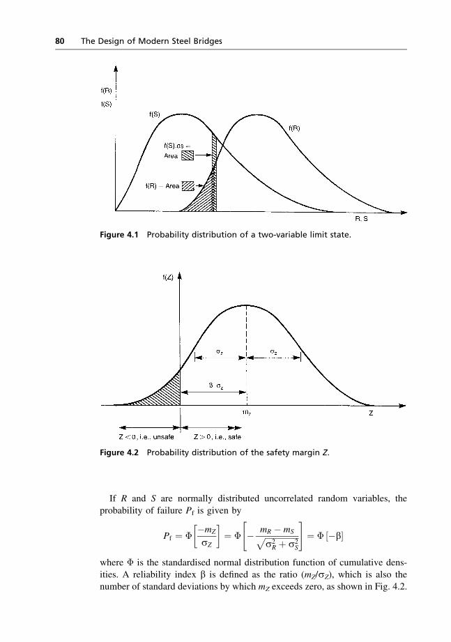
If R and S are normally distributed uncorrelated random variables, the

probability of failure Pf is given by

Pf ¼ ��mZ

sZ

� �¼ � � mR � mSffiffiffiffiffiffiffiffiffiffiffiffiffiffiffiffiffi

s2R þ s2

S

p" #

¼ � ½�b�

where � is the standardised normal distribution function of cumulative dens-

ities. A reliability index b is defined as the ratio (mZ/sZ), which is also thenumber of standard deviations by which mZ exceeds zero, as shown in Fig. 4.2.

Figure 4.1 Probability distribution of a two-variable limit state.

Figure 4.2 Probability distribution of the safety margin Z.


If the basic variables R and S are replaced by a pair of reduced variables oR

and oS given by

oR ¼ R� mR

sR

oS ¼ S� mS

sS

then the failure condition gðoR,oSÞ¼ 0 is given by the equation of the straightline

gðoR,oSÞ ¼ oRsR þ mR � oSsS � mS ¼ 0

This is shown in Fig. 4.3.The frequency of occurrence of a particular value x of a normally distributed

variable is given by the density function

f ðxÞ ¼ 1

sffiffiffiffiffiffi2p

p e�ð1=2Þðx�m=sÞ2

where m and s are the mean value and the standard deviation. Expressed in

reduced coordinate o¼ (x�m)/s, the frequency of a particular value occur-ring is proportional to eð1=2Þo

2. With two uncorrelated normally distributed

variables, the frequency of occurrence of a particular set of values oR and oS

Figure 4.3 Failure condition in the space of two reduced variables.

Aims of Design 81

will thus be proportional to

e�ð1=2Þo2R � e�ð1=2Þo2

S ¼ e�ð1=2Þðo2Rþo2

SÞ

In the space of the reduced variables, the locus of the point of equal frequencywill thus be a circle around the origin, larger radius representing lower fre-

quency. These circles are shown in Fig. 4.3.In Fig. 4.3 a vector OA is drawn from the origin normal to the failure

boundary. OA is thus the shortest distance from the origin to the failure line.Point A represents the most likely set of values of oR and oS for the occurrence

of failure and is thus called the ‘design point’. It can be shown that the lengthof the vector OA is given by

mR � mSffiffiffiffiffiffiffiffiffiffiffiffiffiffiffiffiffis2R þ s2

S

pand is thus numerically equal to the reliability index b.The coordinates of the point A in the space of oR and oS can be shown to be

�ðmR � mSÞsR

ðs2R þ s2

SÞ,ðmR � mSÞsS

ðs2R þ s2

SÞ� �

which can also be expressed as ðaRb, aSbÞ when

aR ¼ � @g@oR

@g@oR

� 2þ @g

@oS

� 2� �1=2 , aS ¼� @g

@oS

@g@oR

� 2þ @g

@oS

� 2� �1=2

The design of new structures can be performed by considering any point onthe horizontal axis of R or S in Fig. 4.1 and its associated probability densityvalues of R and S. Alternatively, the distance of the point from the mean values

of R and S in multiples of the respective standard deviation may be used. Forthe sake of convenience, the ‘design point’ can be chosen for this purpose, as

this point represents the most likely situation at failure.Converting the reduced variables oR and oS to basic variables R and S, the

values of the latter at the ‘design point’ are

Rd ¼ mR þ oRsR ¼ mR þ aRbsR

Sd ¼ mS þ oSsS ¼ mS þ aSbsS

Usually the resistance and action-effect variables R and S of a structure are

functions of a number of variables x1, x2, . . ., xn, and the probability densityfunctions f(R) and f(S) depend upon the probability density functions of the

individual variables x1, etc. and how they are related in the functions R and S.Some of the variables may be common to both, causing some correlation; this

has to be taken into account by modifying the statistical parameters by thecorrelation coefficient. All the basic variables may be replaced by a new set of


reduced variables defined by

oi ¼ xi � mxi

sxi

where mxi and sxi are the mean and the standard deviation of the basic variable

xi. The failure condition may then be written as

gðo1, o2, . . . , onÞ ¼ 0

This equation will represent the failure surface in the multi-dimensional spaceof the reduced variables oi. The reliability index b is the shortest distance fromthe origin to the failure surface. The failure surface is often curved; it is then

necessary to try several points on the curved surface to obtain the shortestvector OA that is also normal to the failure surface. This is equivalent to

linearising the failure surface at the design point by means of, say, Taylor’sseries. The coordinates of the design point are given by oi ¼ aib, when

ai ¼� @g

@oi

� P @g

@oi

� 2� �1=2

calculated at the design point. ai is dependent upon the sensitivity of the failureequation to variation in the variable oi in the region of the design point. ai isproportional to si in the case of planar failure surface; also, for non-planarfailure surfaces, si has a big influence on ai. It may be noted that �a2i ¼ 1.

The values of the basic variables represented by the design point are

xdi ¼ mxi þ aibsxi

The partial safety factor gi for each basic variable xi is the ratio of its ‘design’

value given above to a ‘nominal’ value or a ‘characteristic’ value given in acode. A nominal value is usually based on past practice, without any statisticalanalysis of the probability of its occurrence. A characteristic value xki corres-

ponds to a stipulated probability of non-compliance, usually 5%, and is deter-mined by statistical analysis of test or measurement data; it is given by

xki ¼ mxi þ kisxi

where ki is the number of standard deviations, depending on the stipulatedprobability of non-compliance and the nature of the probability distribution of

the variable xi. For example, for a 95% characteristic value of a normally dis-tributed variable (i.e. 5% probability of non-compliance) ki ¼ 1.64. Obviously,

ki is to be taken with the same sign as ai. Thus

gi ¼xdixki

¼ mxi þ aibsxi

mxi þ kisxi¼ 1þ aibvxi

1þ kivxi

where vxi is the coefficient of variation of the variable xi, equal to sxi=mxi.

Aims of Design 83

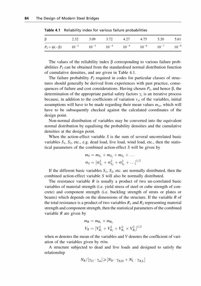
The values of the reliability index b corresponding to various failure prob-abilities Pf can be obtained from the standardised normal distribution function

of cumulative densities, and are given in Table 4.1.The failure probability Pf required in codes for particular classes of struc-

tures should generally be derived from experiences with past practice, conse-quences of failure and cost considerations. Having chosen Pf, and hence b, thedetermination of the appropriate partial safety factors gi is an iterative processbecause, in addition to the coefficients of variation vxi of the variables, initial

assumptions will have to be made regarding their mean values mxi, which willhave to be subsequently checked against the calculated coordinates of thedesign point.

Non-normal distribution of variables may be converted into the equivalentnormal distribution by equalising the probability densities and the cumulative

densities at the design point.When the action-effect variable S is the sum of several uncorrelated basic

variables S1, S2, etc., e.g. dead load, live load, wind load, etc., then the statis-tical parameters of the combined action-effect S will be given by

mS ¼ mS1 þ mS2 þ mS3 þ . . .

sS ¼ ½s2S1þ s2

S2þ s2

S3þ . . .�1=2

If the different basic variables S1, S2, etc. are normally distributed, then the

combined action-effect variable S will also be normally distributed.The resistance variable R is usually a product of two un-correlated basic

variables of material strength (i.e. yield stress of steel or cube strength of con-crete) and component strength (i.e. buckling strength of struts or plates or

beams) which depends on the dimensions of the structure. If the variable R ofthe total resistance is a product of two variables R1 and R2 representing material

strength and component strength, then the statistical parameters of the combinedvariable R are given by

mR ¼ mR1� mR2

VR ¼ ½V2R1þ V2

R2þ V2

R1� V2

R2�1=2

when m denotes the mean of the variables and V denotes the coefficient of vari-

ation of the variables given by s/m.A structure subjected to dead and live loads and designed to satisfy the

relationship

NR=½gf3 � gm�5½ND � gfLD þ NL � gfLL�

Table 4.1 Reliability index for various failure probabilities

b 2.32 3.09 3.72 4.27 4.75 5.20 5.61

Pf¼f(�b) 10�2 10�3 10�4 10�5 10�6 10�7 10�8


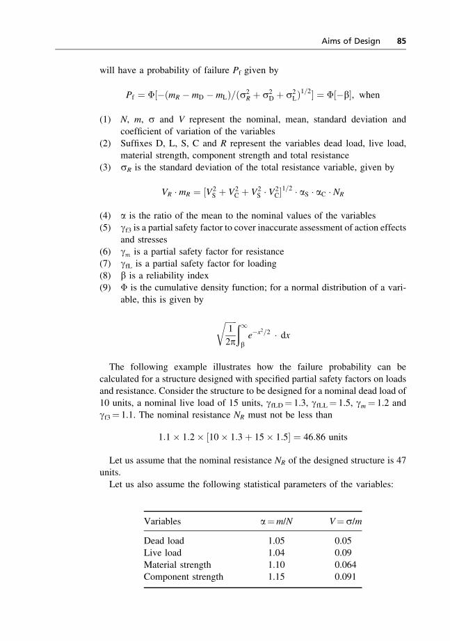
will have a probability of failure Pf given by

Pf ¼ �½�ðmR � mD � mLÞ=ðs2R þ s2

D þ s2LÞ1=2� ¼ �½�b�, when

(1) N, m, s and V represent the nominal, mean, standard deviation andcoefficient of variation of the variables

(2) Suffixes D, L, S, C and R represent the variables dead load, live load,material strength, component strength and total resistance

(3) sR is the standard deviation of the total resistance variable, given by

VR � mR ¼ ½V2S þ V2

C þ V2S � V2

C�1=2 � aS � aC � NR

(4) a is the ratio of the mean to the nominal values of the variables

(5) gf3 is a partial safety factor to cover inaccurate assessment of action effectsand stresses

(6) gm is a partial safety factor for resistance(7) gfL is a partial safety factor for loading

(8) b is a reliability index(9) � is the cumulative density function; for a normal distribution of a vari-

able, this is given by

ffiffiffiffiffiffi1

2p

r ð1be�x2=2 � dx

The following example illustrates how the failure probability can be

calculated for a structure designed with specified partial safety factors on loadsand resistance. Consider the structure to be designed for a nominal dead load of

10 units, a nominal live load of 15 units, gfLD¼ 1.3, gfLL¼ 1.5, gm ¼ 1.2 andgf3¼ 1.1. The nominal resistance NR must not be less than

1:1� 1:2� ½10� 1:3þ 15� 1:5� ¼ 46:86 units

Let us assume that the nominal resistance NR of the designed structure is 47units.

Let us also assume the following statistical parameters of the variables:

Variables a¼m/N V¼s/m

Dead load 1.05 0.05Live load 1.04 0.09

Material strength 1.10 0.064Component strength 1.15 0.091

Aims of Design 85

We can calculate the following statistical properties of the variables dead

and live loads

mD ¼ 1:05� 10 ¼ 10:5 units

sD ¼ 0:05� 10:5 ¼ 0:525 units

mL ¼ 1:04� 15 ¼ 15:6 units

sL ¼ 0:09� 15:6 ¼ 1:404 units

The statistical properties of the resistance variable can be calculated asfollows:

mR ¼ aS � aC � NR ¼ 1:10� 1:15� 47 ¼ 59:455 units

sR ¼ ½V2S þ V2

C þ V2S � V2

C�1=2 � mR

¼ ½0:0642 þ 0:0912 þ 0:0642 � 0:0912�1=2 � 59:455

¼ 6:6233 units

Hence the reliability index b

¼ ½59:455� ð10:5þ 15:6Þ�=½6:62332 þ 0:5252 þ 1:4042�1=2¼ 33:355=6:7908 ¼ 4:912

The failure probability Pf¼ 1� 0.965491¼ 0.45�10�6.

4.5 Partial safety factors in BS 5400

The British bridge code BS 5400[5] uses the Level I method (see Section 4.3)

in its treatment of the two limit states of collapse and serviceability. The safetyfactor format used is

R5S

where

R ¼ design resistance, defined as:

1/gm [function of material strength fk and geometrical parameters of thestructural components]

S ¼ design load effect, defined as:

gf3 (effects of gfL Qk), whereQk ¼ nominal or characteristic loads

fk ¼ characteristic strength of the materialgfL¼ gf1� gf2gf1 ¼ a partial safety factor to take account of the probability of the actual

loads being higher than their characteristic values

gf2 ¼ a partial safety factor to take account of the possibility that, when variousloads act simultaneously, each one of them may not be at the level of its

characteristic value at the same time


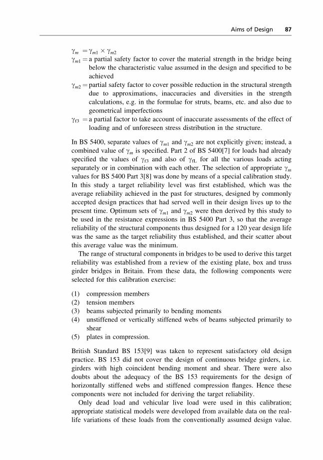
gm ¼ gm1 � gm2gm1 ¼ a partial safety factor to cover the material strength in the bridge being

below the characteristic value assumed in the design and specified to be

achievedgm2 ¼ partial safety factor to cover possible reduction in the structural strength

due to approximations, inaccuracies and diversities in the strengthcalculations, e.g. in the formulae for struts, beams, etc. and also due to

geometrical imperfectionsgf3 ¼ a partial factor to take account of inaccurate assessments of the effect of

loading and of unforeseen stress distribution in the structure.

In BS 5400, separate values of gm1 and gm2 are not explicitly given; instead, a

combined value of gm is specified. Part 2 of BS 5400[7] for loads had alreadyspecified the values of gf3 and also of gfL for all the various loads acting

separately or in combination with each other. The selection of appropriate gmvalues for BS 5400 Part 3[8] was done by means of a special calibration study.

In this study a target reliability level was first established, which was theaverage reliability achieved in the past for structures, designed by commonlyaccepted design practices that had served well in their design lives up to the

present time. Optimum sets of gm1 and gm2 were then derived by this study tobe used in the resistance expressions in BS 5400 Part 3, so that the average

reliability of the structural components thus designed for a 120 year design lifewas the same as the target reliability thus established, and their scatter about

this average value was the minimum.The range of structural components in bridges to be used to derive this target

reliability was established from a review of the existing plate, box and trussgirder bridges in Britain. From these data, the following components were

selected for this calibration exercise:

(1) compression members

(2) tension members(3) beams subjected primarily to bending moments

(4) unstiffened or vertically stiffened webs of beams subjected primarily toshear

(5) plates in compression.

British Standard BS 153[9] was taken to represent satisfactory old design

practice. BS 153 did not cover the design of continuous bridge girders, i.e.girders with high coincident bending moment and shear. There were also

doubts about the adequacy of the BS 153 requirements for the design ofhorizontally stiffened webs and stiffened compression flanges. Hence these

components were not included for deriving the target reliability.Only dead load and vehicular live load were used in this calibration;

appropriate statistical models were developed from available data on the real-life variations of these loads from the conventionally assumed design value.

Aims of Design 87

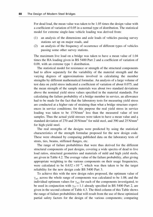
For dead load, the mean value was taken to be 1.05 times the design value with

a coefficient of variation of 0.05 in a normal type of distribution. The statisticalmodel for extreme single-lane vehicle loading was derived from:

(1) an analysis of the dimensions and axle loads of vehicles passing survey

stations set up on major roads, and(2) an analysis of the frequency of occurrence of different types of vehicles

passing some other survey stations.

The maximum live load on a bridge was taken to have a mean value of 1.04

times the HA loading given in BS 5400 Part 2 and a coefficient of variation of0.09, with an extreme type 1 distribution.

The statistical model for resistance or strength of the structural componentshad to allow separately for the variability of the material strength and the

varying degrees of approximations involved in calculating the memberstrengths by different mathematical formulae. An analysis of a large volume of

test data on yield stress indicated a coefficient of variation of about 0.075, andthe mean strength of the sample materials was about two standard deviations

above the nominal yield stress values specified in the material standards. Forcalculating the failure probability of a bridge member in service, an allowancehad to be made for the fact that the laboratory tests for measuring yield stress

are conducted at a higher rate of straining than what a bridge structure experi-ences in service conditions; for this purpose the real yield stress in service

loading was taken to be 15N/mm2 less than the measured value of testsamples. Thus the actual yield stresses were taken to have a mean value and a

standard deviation of 270 and 20N/mm2 for mild steel, and 390 and 25N/mm2

for high-yield steel.

The real strengths of the designs were predicted by using the statisticalcharacteristics of the strength formulae proposed for the new design code.These were obtained by comparing published data on the laboratory tests of

struts, ties, beams, stiffened flanges, etc.The range of failure probabilities that were thus derived for the different

structural components of past designs, covering a wide spectra of dead to liveload ratios, structural geometries and materials of mild and high yield steels,

are given in Table 4.2. The average value of the failure probability, after givingappropriate weighting to the various components on their usage frequencies,

were calculated to be 0.632�10�6, which was then taken to be the targetreliability for the new design code BS 5400 Part 3.

To achieve this with the new design rules proposed, the optimum value ofgm1 across the whole range of components was calculated to be 1.08; and theindividual optimum values for gm2 for each of the components investigated, to

be used in conjunction with gf3¼ 1.1 already specified in BS 5400 Part 2, aregiven in the second column of Table 4.3. The third column of this Table shows

the range of failure probabilities that will result from the use of these optimisedpartial safety factors for the design of the various components; comparing


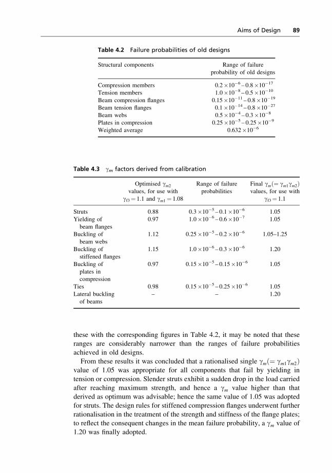
these with the corresponding figures in Table 4.2, it may be noted that theseranges are considerably narrower than the ranges of failure probabilities

achieved in old designs.From these results it was concluded that a rationalised single gmð¼ gm1gm2Þ

value of 1.05 was appropriate for all components that fail by yielding intension or compression. Slender struts exhibit a sudden drop in the load carried

after reaching maximum strength, and hence a gm value higher than thatderived as optimum was advisable; hence the same value of 1.05 was adoptedfor struts. The design rules for stiffened compression flanges underwent further

rationalisation in the treatment of the strength and stiffness of the flange plates;to reflect the consequent changes in the mean failure probability, a gm value of

1.20 was finally adopted.

Table 4.2 Failure probabilities of old designs

Structural components Range of failureprobability of old designs

Compression members 0.2�10�6 – 0.8�10�17

Tension members 1.0�10�8 – 0.5�10�10

Beam compression flanges 0.15�10�11 – 0.8�10�19

Beam tension flanges 0.1�10�14 – 0.8�10�27

Beam webs 0.5�10�4 – 0.3�10�8

Plates in compression 0.25�10�5 – 0.25�10�9

Weighted average 0.632�10�6

Table 4.3 gm factors derived from calibration

Optimised gm2values, for use with

gf3¼ 1.1 and gm1 ¼ 1.08

Range of failureprobabilities

Final gmð¼ gm1gm2Þvalues, for use with

gf3¼ 1.1

Struts 0.88 0.3�10�5 – 0.1�10�6 1.05Yielding ofbeam flanges

0.97 1.0�10�6 – 0.6�10�7 1.05

Buckling ofbeam webs

1.12 0.25�10�5 – 0.2�10�6 1.05–1.25

Buckling ofstiffened flanges

1.15 1.0�10�6 – 0.3�10�6 1.20

Buckling ofplates incompression

0.97 0.15�10�5 – 0.15�10�6 1.05

Ties 0.98 0.15�10�5 – 0.25�10�6 1.05Lateral bucklingof beams

– – 1.20

Aims of Design 89

Buckling of compression flanges of laterally unsupported beams could not

be included in the derivation of the target reliability, as the available statisticaldata on the modelling uncertainty were considered to be inconsistent. After

further research into these data, a gm value of 1.20 was adopted for the designrules in the year 1982 version of reference[8]. The buckling strength formula

for laterally unsupported beams was changed in the year 2000 version ofreference[8], and gm to be used in conjunction with the latest formula has been

specified as 1.05. For buckling of webs of beams in shear, a gm value of 1.05was considered appropriate for webs of low slenderness which fail primarily by

yielding, while a gm value of about 1.25 was required for very slender websthat fail by the tension-field mechanism. In the design rules, a gm value of 1.05was stipulated, along with a variable adjustment factor incorporated in the

strength formula. The calibration exercise showed that the use of these gmfactors and the strength formulae given in BS 5400 Part 3, along with the gfLand gf3 factors given in BS 5400 Part 2, would require approximately 6% lesssteel than in the previous design practice, while achieving the same degree of

reliability on average. Another benefit was the very significant reduction in thescatter of the failure probability about this mean value, as can be seen from

Table 4.3.

References

1. Building Code Requirements for Reinforced Concrete (ACI 318–77). American

Concrete Institute, 1977.

2. Specifications for the Design, Fabrication and Erection of Steel Buildings.

American Institute of Steel Construction, 1978.

3. AASHTO Standard Specifications for Highway Bridges, American Association of

State Highway and Transportation Officials, 1996.

4. CP 110: Part 1: 1972. The Structural Use of Concrete. British Standards Institution,

London.

5. BS 5400: Part 1: 1978. Steel, Concrete and Composite Bridges. British Standards

Institution, London.

6. Flint A. R. et al. 1981. The Design of Steel Bridges. Paper 2: The derivation of

safety factors for design of highway bridges. Granada, London.

7. BS 5400: Part 2: 1978. Steel, Concrete and Composite Bridges: Specification for

Loads. British Standards Institution, London.

8. BS 5400: Part 3: 1982: Code of Practice for Design of Steel Bridges. British

Standards Institution, London.

9. BS 153: 1958. Specification for Steel Girder Bridges. British Standards Institution,

London.


Chapter 5

Rolled Beam and PlateGirder Design

5.1 General features

Rolled I-section steel joists and universal beams are very convenient for

bridges of up to 25m span. Apart from a pair of vertical stiffeners over theirend supports, these do not require any other fabrication. For longer spans,

I-section girders made up of plates are used. Before welding became popular,flange plates were connected to a web plate by riveting through angles, as

shown in Fig. 5.1(a); where a single flange plate was not adequate, severalplates were used as shown in Fig. 5.1(b).

As the bending moment fell along the span, the outer plates were stopped or‘curtailed’. Welding removed the need for the flange angles and also removed

the gaps between adjacent elements where water could collect and initiaterusting (see Fig. 5.1(c)). Curtailment of the flange area is achieved in weldedconstruction by using thinner and/or narrower flange plates in regions of

reduced bending moments, butt-welded to each other at the ends. There is a limitto the thickness of the flange plate that can be conveniently used, since material

properties like weldability, notch toughness, through-thickness ductility andeven yield stress deteriorate with increase in thickness, and risks of lamination

and other inclusions increase. When a single plate is not adequate, the requiredflange area is provided by using several flange plates as shown in Fig. 5.1(d); the

outer plates are made successively narrower than the inner ones, to which theyare connected by fillet welds along the longitudinal edges. The outer plates arediscontinued as the bendingmoments fell along the span; the discontinuity at the

end of each curtailed flange plate is, however, a potential fatigue problem andneeds careful detailing.

There may be other variations and combinations; for example, the flangemay be made up of several plates riveted together and then welded to the web

plate; the web may be made up of two thicker plates near the flanges and onethinner plate at the middle of the cross-section, butt-welded to each other along

the longitudinal edges; the web depth may be varied along the span. Instead ofa plate, a channel section may be used as the flange.

91

Sometimes inclined plates are attached between the flange and the web, asshown in Fig. 5.1(e); they support the flange tip, as well as acting as a

longitudinal stiffener to the web, and more importantly, they provide sometorsional rigidity to the girder.

The material in the web is not as efficient as that in the flange in resistingbending moment. But the shear resistance of an I-beam is related only to the

web area, and thus determines the minimum web area. The most efficientdesign of a plate girder cross-section is thus to make the web as thin and deep

Figure 5.1 Different types of plate girders.


as possible. But deep and thin webs are liable to buckling and may require

stiffening. Vertical stiffeners are provided for the webs to improve theirbuckling resistance, and in the case of very deep and thin webs horizontal

stiffeners may also be necessary. Increased depth of beams also adds to thecost and length of the embankments in the bridge approaches.

The concrete deck on top of the top flange may be made integral with a plategirder by means of shear connectors. Plate girders are used in continuous spans

by splicing adjacent lengths by either bolting or welding. Where the bridgeconsists of several spans, a decision has to be made whether to provide simply

supported girders over each span or to make the girders continuous over severalspans. The advantages of simply supported spans are:

(1) Relative settlement of any support will not change the dead load stresses.

(2) If each span length is within the limits of transportation, then site splicingof girders is avoided.

(3) Expansion joints at the ends of the spans have to cope with the expansionof a single span length only.

The advantages of continuous spans are:

(1) The number of expansion joints can be reduced, often to only one;however, the joint will have to cope with the expansion of several spanlengths. Expansion joints tend to deteriorate with traffic and cause

bumpiness of riding and are potential sources of trouble.(2) The forces due to braking and acceleration of vehicles (see Chapter 3) can

be resisted at one bridge support or shared between several supports; inthe case of simple spans these same forces are to be resisted fully at

several supports and cannot be shared.(3) The number of bearings will be reduced on each pier, which can therefore

be narrowed in elevation.(4) The structure will be generally more rigid, with reduced deflections and

vibrations.(5) There is scope and engineering justification for increasing the girder

depths over supports, thus improving the appearance of the bridge.

(6) Finally, materials in the girder can be reduced and longer spans can bebuilt with fewer piers, thus achieving overall economy.

There is another arrangement of suspended and cantilever spans, as shown in

Fig. 1.1. This arrangement has the advantages (5) and (6) of the continuousspans, the number of expansion joints being less than for simple spans but

more than for continuous spans; each support takes half the longitudinal forcesand carries only one bearing, and like simple spans is unaffected by anysettlement of supports. This arrangement is thus particularly suitable for bridge

sites vulnerable to foundation settlements, e.g. in mining areas.The AASHTO specification[1] requires a minimum depth of steel beams as

1/25 of simple spans, or of the distance between points of contraflexure under

Rolled Beam and Plate Girder Design 93

dead load in the case of continuous construction. For composite beams the

above limit applies to the overall depth, i.e. concrete slab plus steel girder, andthere is an additional limit of 1/30 for the depth of the steel cross-section.

There are also limits on the deflection under live load and impact, which oftengovern the depth of cross-section; these are 1/800 of the span generally, but

1/1000 of the span for bridges in urban areas used by pedestrians. Whereseveral longitudinal girders are interconnected by crossbracings or diaphragms

for efficient lateral distribution of load, the deflection for this purpose may becalculated by assuming that all the girders will deflect equally.

There are no specific limitations on girder depths or deflections in the BritishStandard[2], except that attention is drawn to the need for camber for the sakeof appearance, drainage and headroom clearance. In the case of a nominally

straight bridge, a sagging deflection exceeding 1/800 of the span is alsodiscouraged.

5.2 Analysis for forces and moments

To design a plate girder, it is necessary to first obtain the bending moment,shear force and axial force acting on its various sections. The open cross-section of a plate girder is torsionally very flexible and hence it is generally

assumed that a plate girder section cannot resist any torsion. Axial force occursin a plate girder when the bridge deck is subjected to longitudinal forces due to,

say, braking. Owing to vertical loads, axial force occurs when the plate girderis part of a portal frame or is supported by inclined cables.

If any load is applied over one side of the bridge deck, the beams directlyunder the load obviously deflect more than the others; the consequent trans-

verse bending of the deck slab distributes some of the load on to beams awayfrom the load. This transverse sharing of the load may be further improved by

the provision of transverse diaphragms across the width of the bridge deck andconnected to the longitudinal beams. Transverse diaphragms over the supportsof the longitudinal beams prevent the latter from twisting and are virtually

essential. The usefulness of intermediate diaphragms should be judged bybalancing the improved lateral distribution of load against the cost of provid-

ing, connecting and maintaining them.In a bridge deck constituted by a set of plate girders supporting a concrete

deck, the most convenient way to obtain the bending moments and shear forcesis by the assumption that the deck consists of a grillage of longitudinal and

transverse beams. The continuous concrete slab is replaced by a series ofdiscrete parallel beams spanning between the steel beams. If there are trans-verse members connected to the main longitudinal girders, then the grillage

consists of these longitudinal and transverse girders. Generally the concretedeck is made to act compositely with the steel girders by the provision of shear

connectors; in such cases the concrete slab is taken as a flange of the steel


beam, with an effective area equal to the gross area of the slab between the

steel girders divided by the modular ratio (i.e. the ratio between Young’smoduli of steel and concrete). Sometimes the transverse girders are uncon-

nected to the concrete deck; the grillage analysis in such cases must take intoaccount two separate sets of transverse members, i.e. the concrete slab and the

unconnected steel transverse girders. Shear deformation is generally ignored ingrillage analysis.

Open cross-sections like I-beams have negligible torsional stiffness. Thetorsional stiffness of a concrete slab is also generally ignored, but may be taken

into account by assuming the St Venant torsional constant as d3/6 per unitwidth in the two orthogonal directions, when d is the slab depth.Computer programs for grillage analysis can also easily deal with multiple-

span continuous structures with constant or varying moments of inertia of thelongitudinal girders. The hogging moment over intermediate supports of the

longitudinal girders may cause transverse cracking of the concrete slab in theseregions, thus causing a reduction in the effective moments of inertia. This can

be dealt with in one of the following two ways:

(1) A new distribution of bending moments may be determined by neglecting

the concrete in the calculation of the moment of inertia of the beams overthe length over supports where tensile stress in concrete was found toexceed 10% of its specified 28 day compressive strength, or over, say,

15% of the span lengths on each side of the support.(2) The sagging moments in the adjacent spans are increased, without reduc-

ing the hogging moment; the percentage increase is specified in BS5400[13] as 40 times the ratio of the tensile stress in concrete to its

specified 28 day compressive strength.

In the AASHTO specification[1] empirical methods are authorised forobtaining the transverse distribution of wheel loads. For internal longitudinal

beams with spacing S (metres), the bending moment may be calculated by

(1) taking S/1.676 fraction of wheel loads, if S< 4.267m(2) taking the flooring to act as a simple span between longitudinal beams, if

S> 4.267m.

For external longitudinal beams, the flooring may be assumed to act as asimple span between longitudinal beams, except that, where there are four or

more beams, the fraction of wheel loads shall not be less than:

(1) S/1.676, where S4 1.829m

(2) S/(1.219þ 0.25S), where 1.829< S< 4.267.

Shear forces in all beams may be calculated in the same way as bending

moments, except that, for calculating end shear or reaction, the effect ofa wheel load placed near that end of a beam shall always be calculated by

assuming the flooring to act as a simple span. One condition for adopting this


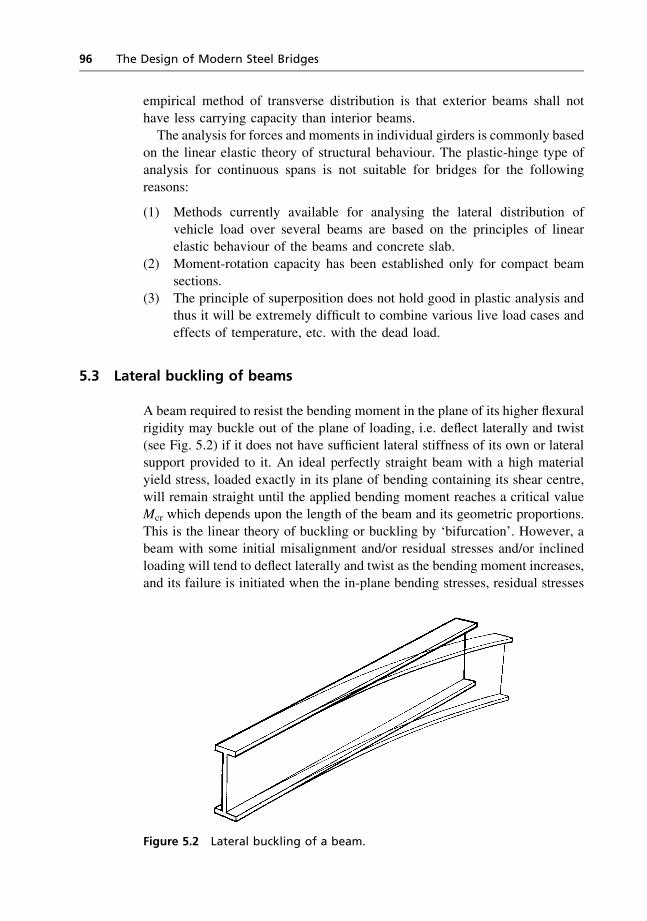
empirical method of transverse distribution is that exterior beams shall not

have less carrying capacity than interior beams.The analysis for forces and moments in individual girders is commonly based

on the linear elastic theory of structural behaviour. The plastic-hinge type ofanalysis for continuous spans is not suitable for bridges for the following

reasons:

(1) Methods currently available for analysing the lateral distribution ofvehicle load over several beams are based on the principles of linearelastic behaviour of the beams and concrete slab.

(2) Moment-rotation capacity has been established only for compact beamsections.

(3) The principle of superposition does not hold good in plastic analysis andthus it will be extremely difficult to combine various live load cases and

effects of temperature, etc. with the dead load.

5.3 Lateral buckling of beams

A beam required to resist the bending moment in the plane of its higher flexuralrigidity may buckle out of the plane of loading, i.e. deflect laterally and twist(see Fig. 5.2) if it does not have sufficient lateral stiffness of its own or lateral

support provided to it. An ideal perfectly straight beam with a high materialyield stress, loaded exactly in its plane of bending containing its shear centre,

will remain straight until the applied bending moment reaches a critical valueMcr which depends upon the length of the beam and its geometric proportions.

This is the linear theory of buckling or buckling by ‘bifurcation’. However, abeam with some initial misalignment and/or residual stresses and/or inclined

loading will tend to deflect laterally and twist as the bending moment increases,and its failure is initiated when the in-plane bending stresses, residual stresses

Figure 5.2 Lateral buckling of a beam.


and stresses caused by lateral deflection and twist combine to cause yielding.

This is the non-linear or ‘divergence’ theory of buckling. The critical bendingmoment of the ideal straight beam with very high yield stress will be discussed

first, and then it will be described how this value is modified to take account ofthe onset of yielding.

5.3.1 Buckling of an ideal beam

The critical bending moment of a perfectly straight elastic beam with cross-section symmetrical about both axes is given by

Mcr ¼ pLe

ffiffiffiffiffiffiffiffiffiffiffiffiffiEIy GJ

a

r ffiffiffiffiffiffiffiffiffiffiffiffiffiffiffiffiffiffiffiffiffi1þ p2 EIw

L2e GJ

sð5:1Þ

where

EIy ¼ flexural rigidity about the minor axis

GJ ¼ torsional rigidityEIw ¼ warping rigidity

Le ¼ half-wavelength of buckling, or ‘effective length’, as it is generallycalled

a ¼ is a correction factor, just less than 1.0, to correct for deflection due to

bending; it is given approximately by ðIx � IyÞ=Ix, where Ix is themajor axis moment of inertia.

For the standard case of a beam of length L subjected to equal and opposite

end moments, restrained at its ends against lateral deflections and twist but freeto rotate in plan, and without any intermediate lateral restraint, Le is equal to L.

Equation (5.1) can also be expressed as

Mcr ¼ p2EL2e

ffiffiffiffiffiffiffiffiIyIwa

r� b ð5:2Þ

where b represents the contribution of the torsional rigidity of the section andis given by

b ¼ffiffiffiffiffiffiffiffiffiffiffiffiffiffiffiffiffiffiffiffi1þ L2eGJ

p2EIw

sð5:3Þ

For equal flange I-sections

Iw ¼ Iyh2

4

where h is the distance between the centroids of the flanges; hence equation(5.2) may be expressed as

Mcr ¼ p2EIy2L2e

hbffiffiffia

p ð5:4Þ


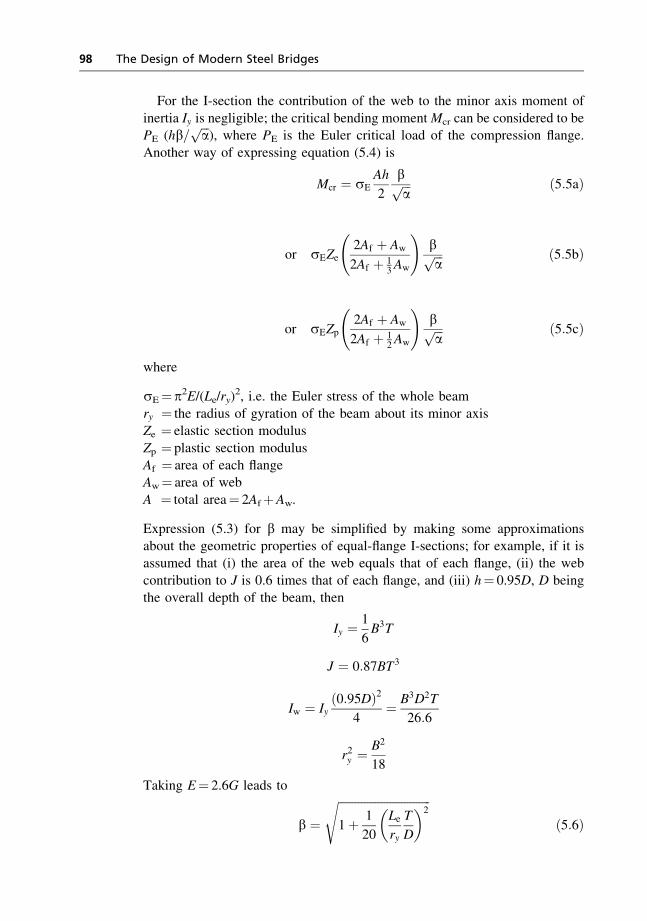
For the I-section the contribution of the web to the minor axis moment of

inertia Iy is negligible; the critical bending momentMcr can be considered to bePE (hb=

ffiffiffia

p), where PE is the Euler critical load of the compression flange.

Another way of expressing equation (5.4) is

Mcr ¼ sEAh

2

bffiffiffia

p ð5:5aÞ

or sEZe2Af þ Aw

2Af þ 13Aw

!bffiffiffia

p ð5:5bÞ

or sEZp2Af þ Aw

2Af þ 12Aw

!bffiffiffia

p ð5:5cÞ

where

sE¼p2E/(Le/ry)2, i.e. the Euler stress of the whole beam

ry ¼ the radius of gyration of the beam about its minor axisZe ¼ elastic section modulus

Zp ¼ plastic section modulusAf ¼ area of each flangeAw¼ area of web

A ¼ total area¼ 2AfþAw.

Expression (5.3) for b may be simplified by making some approximationsabout the geometric properties of equal-flange I-sections; for example, if it isassumed that (i) the area of the web equals that of each flange, (ii) the web

contribution to J is 0.6 times that of each flange, and (iii) h¼ 0.95D, D beingthe overall depth of the beam, then

Iy ¼ 1

6B3T

J ¼ 0:87BT3

Iw ¼ Iyð0:95DÞ2

4¼ B3D2T

26:6

r2y ¼B2

18

Taking E¼ 2.6G leads to

b ¼ffiffiffiffiffiffiffiffiffiffiffiffiffiffiffiffiffiffiffiffiffiffiffiffiffiffiffiffiffiffiffiffi1þ 1

20

Lery

T

D

� �2s

ð5:6Þ


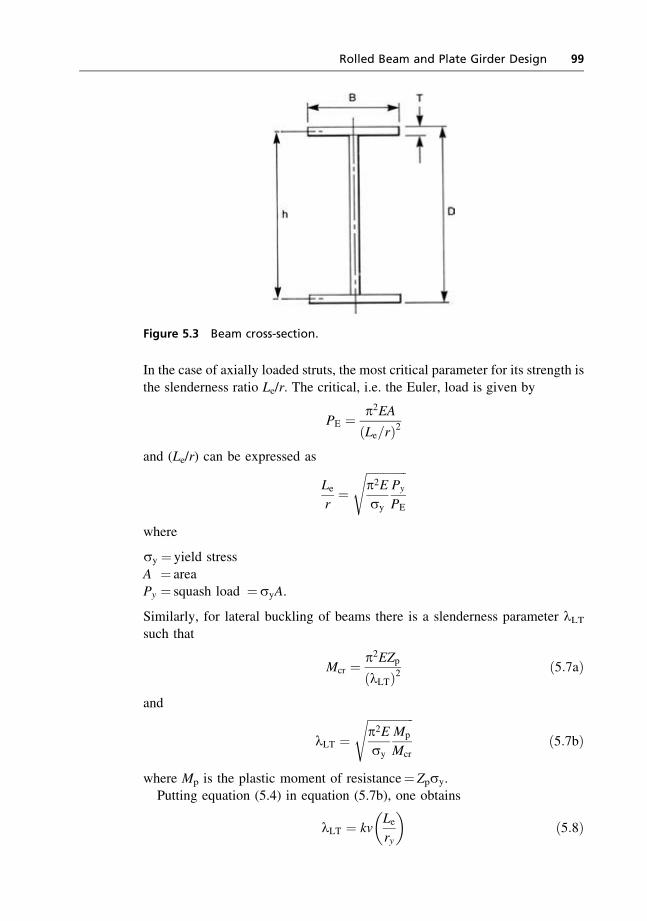
In the case of axially loaded struts, the most critical parameter for its strength is

the slenderness ratio Le/r. The critical, i.e. the Euler, load is given by

PE ¼ p2EA

ðLe=rÞ2

and (Le/r) can be expressed as

Ler¼

ffiffiffiffiffiffiffiffiffiffiffiffiffiffip2Esy

Py

PE

s

where

sy ¼ yield stress

A ¼ areaPy ¼ squash load ¼syA.

Similarly, for lateral buckling of beams there is a slenderness parameter lLTsuch that

Mcr ¼ p2EZpðlLTÞ2

ð5:7aÞ

and

lLT ¼ffiffiffiffiffiffiffiffiffiffiffiffiffiffiffiffip2Esy

Mp

Mcr

sð5:7bÞ

where Mp is the plastic moment of resistance¼ Zpsy.Putting equation (5.4) in equation (5.7b), one obtains

lLT ¼ kvLery

� �ð5:8Þ

Figure 5.3 Beam cross-section.


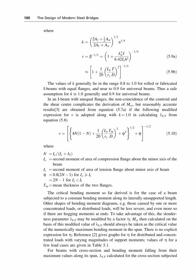
where

k ¼ 2Af þ 12Aw

2Af þ Aw

� �1=2

a1=4

v ¼ b�1=2 ¼ 1þ L2eJ

6:42Iyh2

� ��1=4

ð5:9aÞ

� 1þ 1

20

Lery

T

D

� �2" #�1=4

ð5:9bÞ

The values of k generally lie in the range 0.8 to 1.0 for rolled or fabricatedI-beams with equal flanges, and near to 0.9 for universal beams. Thus a safe

assumption for k is 1.0 generally and 0.9 for universal beams.In an I-beam with unequal flanges, the non-coincidence of the centroid and

the shear centre complicates the derivation of Mcr, but reasonably accurate

results[3] are obtained from equation (5.7a) if the following modifiedexpression for v is adopted along with k¼ 1.0 in calculating lLT from

equation (5.8)

v ¼ 4Nð1� NÞ þ 1

20

Lery

TmD

� �2

þc2

( )1=2

þc

24

35�1=2

ð5:10Þ

where

N ¼ Ic=ðIc þ ITÞIc ¼ second moment of area of compression flange about the minor axis of the

beamIt ¼ second moment of area of tension flange about minor axis of beam

c ¼ 0.8(2N� 1) for Ic5 It¼ 2N� 1 for Ic< It

Tm¼mean thickness of the two flanges.

The critical bending moment so far derived is for the case of a beam

subjected to a constant bending moment along its laterally unsupported length.Other shapes of bending moment diagrams, e.g. those caused by one or more

concentrated loads, or distributed loads, will be less severe, and even more soif there are hogging moments at ends. To take advantage of this, the slender-

ness parameter lLT may be modified by a factor Z; Mcr then calculated on thebasis of this modified value of lLT should always be taken as the critical value

of the numerically maximum bending moment in the span. There is no explicitexpression for Z; Reference [2] gives graphs for Z for distributed and concen-trated loads with varying magnitudes of support moments; values of Z for a

few load cases are given in Table 5.1.For beams with cross-section and bending moment falling from their

maximum values along its span, lLT calculated for the cross-section subjected


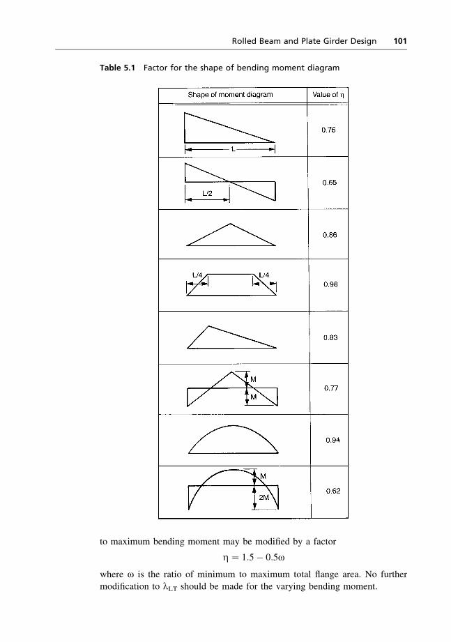
to maximum bending moment may be modified by a factor

Z ¼ 1:5� 0:5o

where o is the ratio of minimum to maximum total flange area. No further

modification to lLT should be made for the varying bending moment.

Table 5.1 Factor for the shape of bending moment diagram


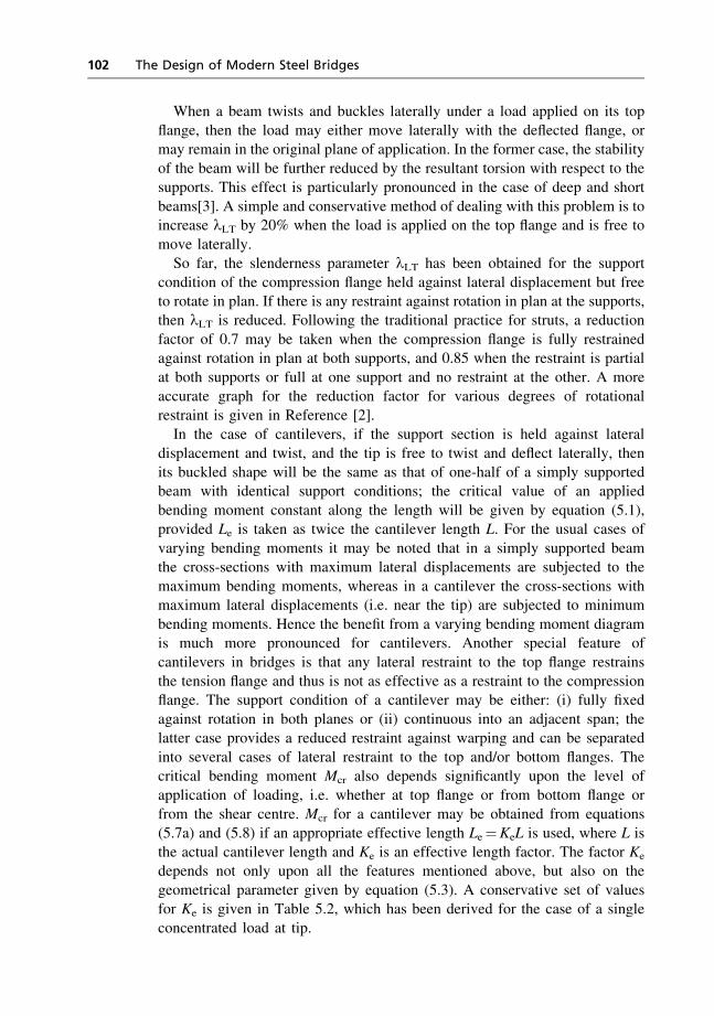
When a beam twists and buckles laterally under a load applied on its top

flange, then the load may either move laterally with the deflected flange, ormay remain in the original plane of application. In the former case, the stability

of the beam will be further reduced by the resultant torsion with respect to thesupports. This effect is particularly pronounced in the case of deep and short

beams[3]. A simple and conservative method of dealing with this problem is toincrease lLT by 20% when the load is applied on the top flange and is free to

move laterally.So far, the slenderness parameter lLT has been obtained for the support

condition of the compression flange held against lateral displacement but freeto rotate in plan. If there is any restraint against rotation in plan at the supports,then lLT is reduced. Following the traditional practice for struts, a reduction

factor of 0.7 may be taken when the compression flange is fully restrainedagainst rotation in plan at both supports, and 0.85 when the restraint is partial

at both supports or full at one support and no restraint at the other. A moreaccurate graph for the reduction factor for various degrees of rotational

restraint is given in Reference [2].In the case of cantilevers, if the support section is held against lateral

displacement and twist, and the tip is free to twist and deflect laterally, thenits buckled shape will be the same as that of one-half of a simply supportedbeam with identical support conditions; the critical value of an applied

bending moment constant along the length will be given by equation (5.1),provided Le is taken as twice the cantilever length L. For the usual cases of

varying bending moments it may be noted that in a simply supported beamthe cross-sections with maximum lateral displacements are subjected to the

maximum bending moments, whereas in a cantilever the cross-sections withmaximum lateral displacements (i.e. near the tip) are subjected to minimum

bending moments. Hence the benefit from a varying bending moment diagramis much more pronounced for cantilevers. Another special feature of

cantilevers in bridges is that any lateral restraint to the top flange restrainsthe tension flange and thus is not as effective as a restraint to the compressionflange. The support condition of a cantilever may be either: (i) fully fixed

against rotation in both planes or (ii) continuous into an adjacent span; thelatter case provides a reduced restraint against warping and can be separated

into several cases of lateral restraint to the top and/or bottom flanges. Thecritical bending moment Mcr also depends significantly upon the level of

application of loading, i.e. whether at top flange or from bottom flange orfrom the shear centre. Mcr for a cantilever may be obtained from equations

(5.7a) and (5.8) if an appropriate effective length Le¼KeL is used, where L isthe actual cantilever length and Ke is an effective length factor. The factor Ke

depends not only upon all the features mentioned above, but also on the

geometrical parameter given by equation (5.3). A conservative set of valuesfor Ke is given in Table 5.2, which has been derived for the case of a single

concentrated load at tip.


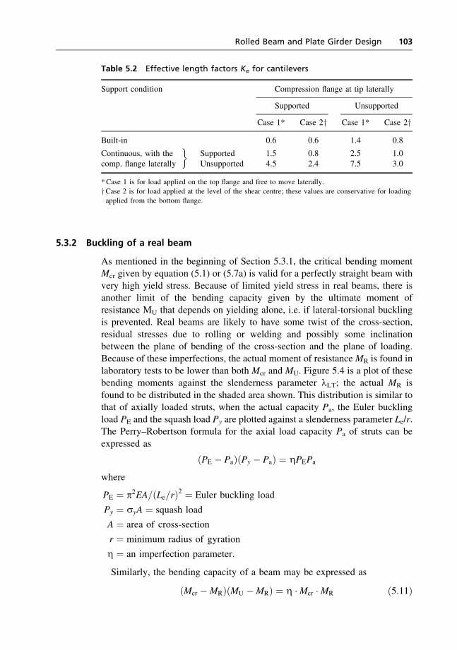
5.3.2 Buckling of a real beam

As mentioned in the beginning of Section 5.3.1, the critical bending momentMcr given by equation (5.1) or (5.7a) is valid for a perfectly straight beam with

very high yield stress. Because of limited yield stress in real beams, there isanother limit of the bending capacity given by the ultimate moment of

resistance MU that depends on yielding alone, i.e. if lateral-torsional bucklingis prevented. Real beams are likely to have some twist of the cross-section,

residual stresses due to rolling or welding and possibly some inclinationbetween the plane of bending of the cross-section and the plane of loading.Because of these imperfections, the actual moment of resistanceMR is found in

laboratory tests to be lower than both Mcr and MU. Figure 5.4 is a plot of thesebending moments against the slenderness parameter lLT; the actual MR is

found to be distributed in the shaded area shown. This distribution is similar tothat of axially loaded struts, when the actual capacity Pa, the Euler buckling

load PE and the squash load Py are plotted against a slenderness parameter Le/r.The Perry–Robertson formula for the axial load capacity Pa of struts can be

expressed as

ðPE � PaÞðPy � PaÞ ¼ ZPEPa

where

PE ¼ p2EA=ðLe=rÞ2 ¼ Euler buckling load

Py ¼ syA ¼ squash load

A ¼ area of cross-section

r ¼ minimum radius of gyration

Z ¼ an imperfection parameter:

Similarly, the bending capacity of a beam may be expressed as

ðMcr �MRÞðMU �MRÞ ¼ Z �Mcr �MR ð5:11Þ

Table 5.2 Effective length factors Ke for cantilevers

Support condition Compression flange at tip laterally

Supported Unsupported

Case 1* Case 2y Case 1* Case 2yBuilt-in 0.6 0.6 1.4 0.8

Continuous, with the�

comp. flange laterallySupported 1.5 0.8 2.5 1.0Unsupported 4.5 2.4 7.5 3.0

*Case 1 is for load applied on the top flange and free to move laterally.

yCase 2 is for load applied at the level of the shear centre; these values are conservative for loading

applied from the bottom flange.


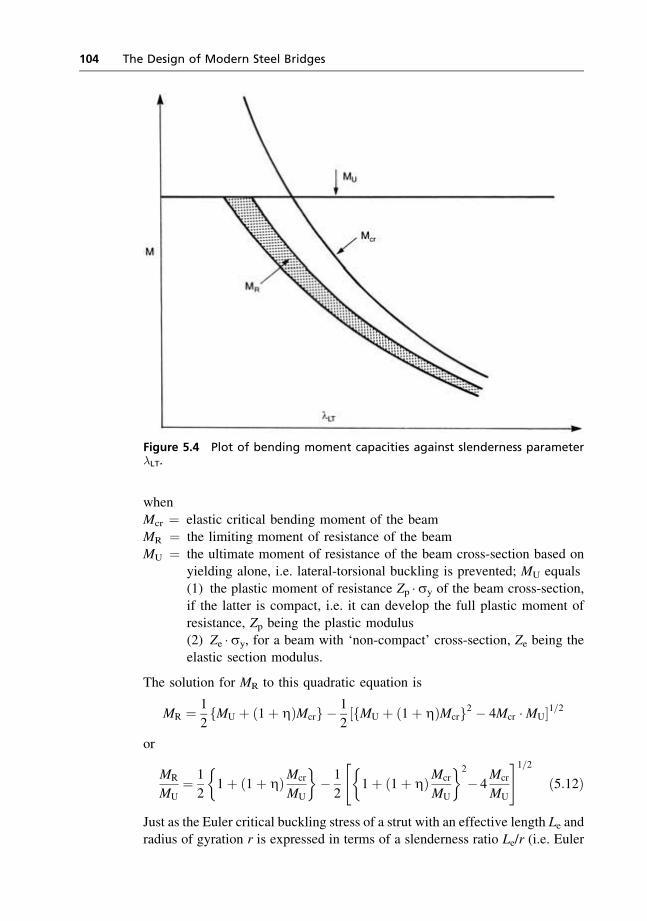
when

Mcr ¼ elastic critical bending moment of the beamMR ¼ the limiting moment of resistance of the beam

MU ¼ the ultimate moment of resistance of the beam cross-section based onyielding alone, i.e. lateral-torsional buckling is prevented; MU equals

(1) the plastic moment of resistance Zp �sy of the beam cross-section,if the latter is compact, i.e. it can develop the full plastic moment of

resistance, Zp being the plastic modulus(2) Ze �sy, for a beam with ‘non-compact’ cross-section, Ze being theelastic section modulus.

The solution for MR to this quadratic equation is

MR ¼ 1

2fMU þ ð1þ ZÞMcrg � 1

2½fMU þ ð1þ ZÞMcrg2 � 4Mcr �MU�1=2

or

MR

MU¼ 1

21þ ð1þ ZÞMcr

MU

� �� 1

21þ ð1þ ZÞMcr

MU

� �2

� 4Mcr

MU

" #1=2ð5:12Þ

Just as the Euler critical buckling stress of a strut with an effective length Le andradius of gyration r is expressed in terms of a slenderness ratio Le/r (i.e. Euler

Figure 5.4 Plot of bending moment capacities against slenderness parameter�LT.


stress is equal to p2E/(Le/r)2), similarly Mcr of a beam can be expressed in

terms of a slenderness parameter lLT as shown in equation (5.7a), namely

Mcr ¼ p2EZp=l2LT

when Zp is the plastic modulus of the section.Then

Mcr

MU¼ p2E

l2LT� ZpMU

The above indicates that Mcr/MU depends not just on lLT, but also on:

(1) sy for compact section

(2) sy, and the ratio of the plastic to elastic modulus, Zp/Ze, for non-compactsection.

We can introduce another slenderness parameter b such that

b2 ¼ l2LT �sy

355�MU

Mp

Then

Mcr

MU¼ p2EZp

MU� syMU

b2 � 355 �Mp

¼ p2E

b2 � 355 ¼ 5700

b2

Using this relationship in equation (5.12) leads to:

MR

MU¼ 1

2

�f1þ ½1þ Z� � 5700=b2g

�ffiffiffiffiffiffiffiffiffiffiffiffiffiffiffiffiffiffiffiffiffiffiffiffiffiffiffiffiffiffiffiffiffiffiffiffiffiffiffiffiffiffiffiffiffiffiffiffiffiffiffiffiffiffiffiffiffiffiffiffiffiffiffiffiffiffiffiffiffiffiffiffiffiffiffif1þ ½1þ Z� � 5700=b2g2 � 22 800=b2

q �ð5:13Þ

Test results indicate that for small values of the slenderness parameter b, viz.less than about 30, the limiting moment of resistance MR is not reduced below

MU, the ultimate moment of resistance based on yielding alone. Theimperfection parameter Z is chosen in such a way as to produce:

(1) MR/MU equal to 1.0 for stocky range (i.e. b-values less than about 30),

and(2) good correlation with test results for higher values of b.

Account should also be taken of the fact that beams fabricated by longitudinally

welding flange and web plates will possess significant longitudinal compres-sive welding residual stresses along various parts of the beam cross-section,

thus possibly bringing about an earlier onset of local compressive yielding andconsequent reduction in flexural stiffness. Reference [2] has adopted the


following expressions for Z:

0:008ðb� 30Þ, for beams fabricated by longitudinal welding

0:0035ðb� 30Þ, for other beams, including stress-relieved

welded beams

ð5:14Þ

Reference [2] has introduced a further refinement for Z to be used in equation

(5.13) for beams with intermediate restraints against lateral-torsional buckling.For such beams the half-wave-length for elastic critical buckling of the

compression flange taken as a strut is longer than the effective length of thatstrut calculated from its elastic critical buckling load (see Section 5.3.3). Onthe hypothesis that the amplitude of imperfection over the half-wave-length of

buckling is more critical than the amplitude of imperfection over a notionaleffective length, b is multiplied by the ratio of the half-wave-length to the

effective length for calculating Z for such beams.Taking equation (5.4) for the critical bending moment Mcr, it may be

conservatively assumed that:

(1) a is equal to unity(2) the torsional rigidity GJ of a beam is very small compared with the

warping rigidity EIw (i.e. b is equal to unity)(3) the longitudinal load in the compression flange is equal to the bending

moment divided by the depth h of the beam between the centroids of thetwo flanges.

This leads to the concept that the permissible stress in the compressionflange of a beam may be taken as that of the compression flange acting as

a strut. The treatment of lateral buckling of a beam in the American code[1] forbridges is based on this concept. The critical buckling stress in the compression

flange is thus taken to be its Euler buckling stress sE given by

sE ¼ p2E

ðLe=rycÞ2ð5:15Þ

where ryc is the radius of gyration of the compression flange about itscentroidal y–y axis; ryc is equal to B/

ffiffiffiffiffi12

pwhere B is the width of the flange.

The effects of imperfection and residual stresses are also treated in the mannerthat was originally developed by the American Column Research Council[4]

for columns. In this approach, the limiting stress sb is related to the Eulerbuckling stress sE by

sb ¼ sy 1� sy

4E

� ð5:16Þ

The above equation was originally meant to be valid in the range sE>sy/2.

For lower values of sE, sb was taken equal to sE; the effects of imperfectionsand residual stresses in this range were covered by a slightly higher safety

factor than those in the range sE>sy/2. In the AASHTO code, however,


equation (5.16) has been adopted for lateral buckling of beams for all values of

sE, with the same safety factor. It may be noted that equation (5.16) results insb¼ 0 for Le/B¼ p

ffiffiffiffiffiffiffiffiffiffiffiffiffiE=3sy

p; the AASHTO code specifies an upper limit of

1.27ffiffiffiffiffiffiffiffiffiffiffiE=sy

pfor Le/B. This code allows the full plastic moment of resistance

(Zpsy) to be taken when Le/ry 4 581/ffiffiffiffiffiffisy

pfor fairly uniform bending moment

(i.e. M25 0.7M1), and Le/ry 4 996/ffiffiffiffiffiffisy

pfor varying bending moment (i.e.

M2< 0.7M1), where Le is the distance between the effective restraints of com-

pression flange, ry is the radius of gyration of the whole beam about its y–y axis,M1 and M2 are the bending moments at the ends of Le and sy is in N/mm2. The

code also allows the full elastic moment of resistance (Zesy) to be taken when

LeD

BT<

137 900

sy

where D, B and T are the depth, flange width and flange thickness, respectively,

of the beam. These limits may be compared with the limit of

b ¼ lLT

ffiffiffiffiffiffiffiffisy

355

r ffiffiffiffiffiffimu

mp

r¼ 30

below which the British code requires no reduction in the limiting bendingcompressive stress due to lateral buckling.

5.3.3 Compression flange with intermediate lateral restraints of limited rigidity

The compression flange can be idealised as a continuous strut elastically res-

trained by springs. Assume a deflected shape of the strut with m number ofsinusoidal half-waves in its total length of L, with amplitude am. The strain

energy of bending of the strut is equal to

EIc2

ðL0

d2y=dx2 � dx ¼ p4EIc4L3

� m4a2m

where Ic is the lateral moment of inertia of the compression flange.

The strain energy of the elastic restraints is equal to

k

2

ðL0

y2 dx ¼ kL

4� a2m

where k is the elastic stiffness of lateral restraints per unit length.Work done by the axial force is equal to

P� shortening of the strut ¼ P � p2

4L� m2a2m

where P is the axial force.

Equating total strain energy to work done

P ¼ p2EIcL2

� m2 þ kL4

p4EIcm2

� �


For minimum value of P, dP/dm¼ 0. This leads to

m ¼ L

p½k=EIc�1=4

Pcr ¼ 2 �ffiffiffiffiffiffiffiffiffiEIck

pL

m¼ critical half-wave-length ¼ p½EIc=k�1=4

The effective length of an equivalent strut with Euler buckling load equal to

the above value of Pcr will be given by

p2EIcl2eff

¼ 2ffiffiffiffiffiffiffiffiffiEIck

p

leading to

leff ¼ pffiffiffi2

p ½EIc=k�1=4

The above results are theoretically valid for a beam under constant bending

moment, but may be conveniently and conservatively used for beams subjectedto varying bending moments, using the maximum compressive flange force forcomparing with the Pcr-value obtained from above.

If the lateral restraints are spaced at s and their flexibility, i.e. deflection dueto unit force at the restraint, is d, then k � s¼ 1/d, and

leff ¼ pffiffiffi2

p ½EIcsd�1=4

The lateral restraints to the compression flange may be in the form of torsionalrestraints, such that a is the rotation of the restraint due to unit torque applied

at that restraint. Then the displacement of one flange with respect to the otherdue to unit forces applied at flange levels of each torsional restraint will be d2a,when d is the depth of the girder between the centroids of its flanges. Theeffective length of the compressive flange can then be obtained by replacing

d by d2a in the previous expression, i.e.

leff ¼ pffiffiffi2

p ½EIcsd2a�1=4

5.3.4 Compression flange with full lateral restraints at ends and one restraint oflimited rigidity at midpoint

Assume a single sinusoidal half-wave of buckling, i.e.

y ¼ a sinðpx=LÞThe strain energy of bending of the flange ¼ p4EIca2=4L3


The strain energy of the elastic restraint at midpoint ¼ sa2=2, where s is the

stiffness of the restraint.Work done by the axial force ¼ p2Pa2=4L, wherefrom

Pcr ¼ p2EIcL2

1þ 2sL3

p4EIc

� �, but not more than 4p2EIc=L2

and

leff ¼ L 1þ 2sL3

p4EIc

� ��1=2

, but not less than 12L:

5.4 Local buckling of plate elements

If a beam is made up of thin plate elements, i.e. thin web or flanges, then theseplate elements may buckle well before the beam section reaches its overallelastic or buckling strength. Elastic buckling theories may be applied to derive

the critical buckling stress of individual plate elements in the beam cross-section, i.e. the magnitude of the applied stress at which an ideal initially flat

residual-stress-free plate becomes unstable and deflects out of its initially flatplane. The critical buckling stress depends upon the pattern of the applied

stress, the geometry of the plate and the out-of-plane restraints on its edges.However, unlike overall buckling of beams and columns, a slender plate

element may carry increased loading beyond the elastic critical value withincreased out-of-plane deflection, i.e. it may have post-buckling strength.

A plate with some initial out-of-flatness starts deflecting out-of-plane rightfrom the beginning of load application, and the rate of deflection increases asthe critical buckling stress is reached; in the post-buckling range the stiffness

of the plate is less than that below the critical buckling level. The stiffness andstrength of a plate element in the post-buckling range depend on the in-plane

restraint at the edges of the plate. As a plate element starts deflecting out-of-plane, the distribution of in-plane stresses due to applied load becomes non-

uniform and, in addition, bending stresses develop. As the combined in-planeand bending stresses reach the elastic limit in some parts of the plate, these

parts lose their stiffness. The ultimate strength of the plate element is reachedwhen a large part of the plate has yielded. Residual stresses in parts of the platedue to welding or rolling may bring about an earlier onset of yielding in these

parts and may lower both the ultimate strength of the plate and its stiffness inthe post-elastic range.


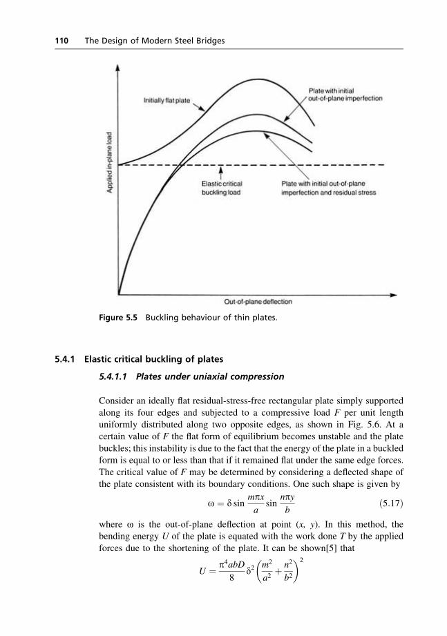
5.4.1 Elastic critical buckling of plates

5.4.1.1 Plates under uniaxial compression

Consider an ideally flat residual-stress-free rectangular plate simply supportedalong its four edges and subjected to a compressive load F per unit length

uniformly distributed along two opposite edges, as shown in Fig. 5.6. At acertain value of F the flat form of equilibrium becomes unstable and the plate

buckles; this instability is due to the fact that the energy of the plate in a buckledform is equal to or less than that if it remained flat under the same edge forces.

The critical value of F may be determined by considering a deflected shape ofthe plate consistent with its boundary conditions. One such shape is given by

o ¼ d sinmpxa

sinnpyb

ð5:17Þ

where o is the out-of-plane deflection at point (x, y). In this method, thebending energy U of the plate is equated with the work done T by the applied

forces due to the shortening of the plate. It can be shown[5] that

U ¼ p4abD8

d2m2

a2þ n2

b2

� �2

Figure 5.5 Buckling behaviour of thin plates.


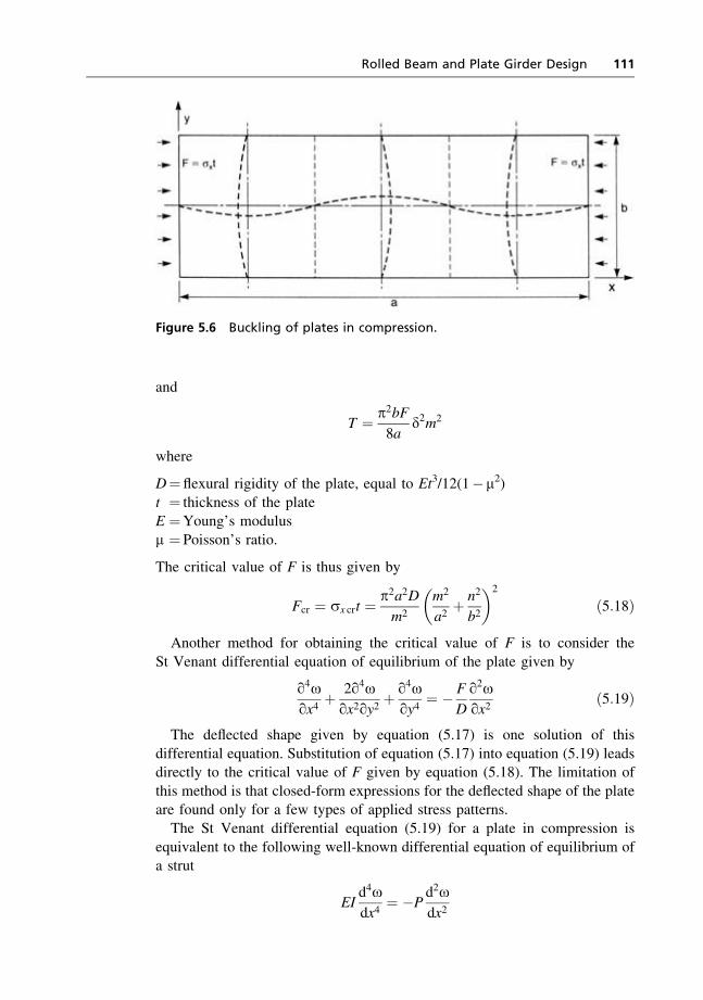
and

T ¼ p2bF8a

d2m2

where

D¼ flexural rigidity of the plate, equal to Et3/12(1�m2)t ¼ thickness of the plateE ¼Young’s modulus

m ¼ Poisson’s ratio.

The critical value of F is thus given by

Fcr ¼ sx crt ¼ p2a2Dm2

m2

a2þ n2

b2

� �2

ð5:18Þ

Another method for obtaining the critical value of F is to consider the

St Venant differential equation of equilibrium of the plate given by

q4oqx4

þ 2q4oqx2qy2

þ q4oqy4

¼ � F

D

q2oqx2

ð5:19Þ

The deflected shape given by equation (5.17) is one solution of this

differential equation. Substitution of equation (5.17) into equation (5.19) leadsdirectly to the critical value of F given by equation (5.18). The limitation of

this method is that closed-form expressions for the deflected shape of the plateare found only for a few types of applied stress patterns.The St Venant differential equation (5.19) for a plate in compression is

equivalent to the following well-known differential equation of equilibrium ofa strut

EId4odx4

¼ �Pd2odx2

Figure 5.6 Buckling of plates in compression.


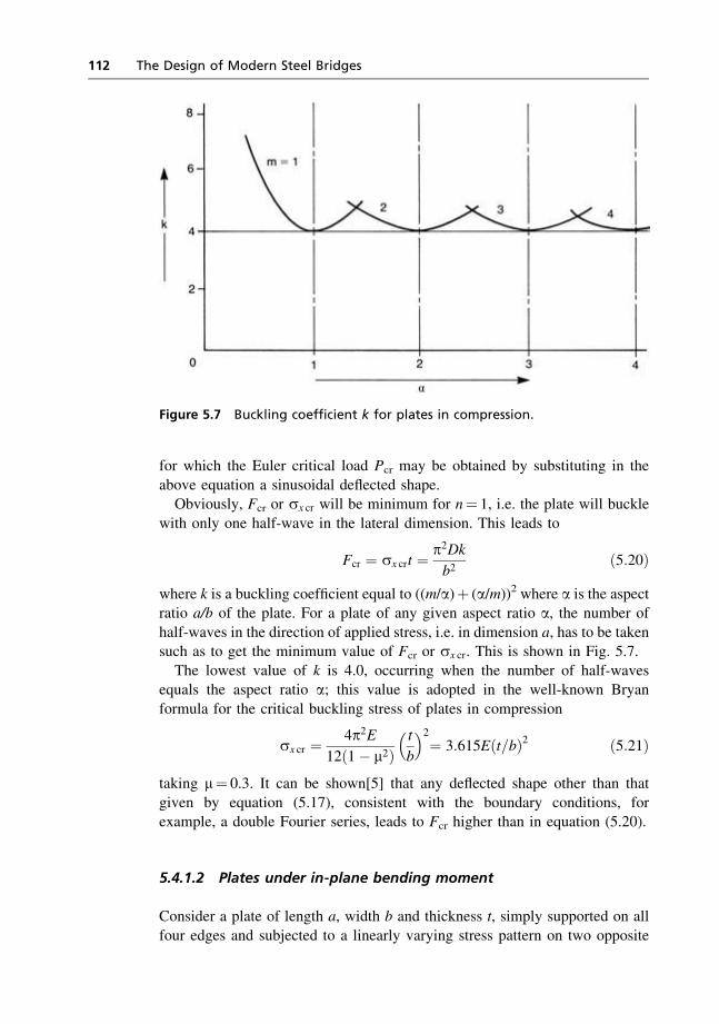
for which the Euler critical load Pcr may be obtained by substituting in the

above equation a sinusoidal deflected shape.Obviously, Fcr or sx cr will be minimum for n¼ 1, i.e. the plate will buckle

with only one half-wave in the lateral dimension. This leads to

Fcr ¼ sx crt ¼ p2Dkb2

ð5:20Þ

where k is a buckling coefficient equal to ((m/a)þ (a/m))2 where a is the aspectratio a/b of the plate. For a plate of any given aspect ratio a, the number of

half-waves in the direction of applied stress, i.e. in dimension a, has to be takensuch as to get the minimum value of Fcr or sx cr. This is shown in Fig. 5.7.

The lowest value of k is 4.0, occurring when the number of half-wavesequals the aspect ratio a; this value is adopted in the well-known Bryan

formula for the critical buckling stress of plates in compression

sx cr ¼ 4p2E12ð1� m2Þ

t

b

� 2¼ 3:615Eðt=bÞ2 ð5:21Þ

taking m¼ 0.3. It can be shown[5] that any deflected shape other than that

given by equation (5.17), consistent with the boundary conditions, forexample, a double Fourier series, leads to Fcr higher than in equation (5.20).

5.4.1.2 Plates under in-plane bending moment

Consider a plate of length a, width b and thickness t, simply supported on all

four edges and subjected to a linearly varying stress pattern on two opposite

Figure 5.7 Buckling coefficient k for plates in compression.


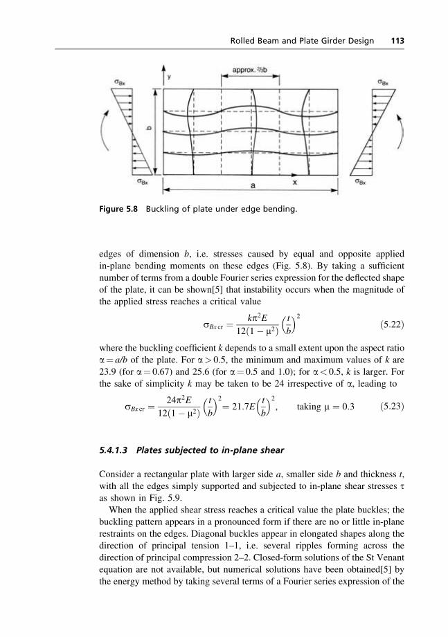
edges of dimension b, i.e. stresses caused by equal and opposite appliedin-plane bending moments on these edges (Fig. 5.8). By taking a sufficient

number of terms from a double Fourier series expression for the deflected shapeof the plate, it can be shown[5] that instability occurs when the magnitude ofthe applied stress reaches a critical value

sBx cr ¼ kp2E12ð1� m2Þ

t

b

� 2ð5:22Þ

where the buckling coefficient k depends to a small extent upon the aspect ratioa¼ a/b of the plate. For a> 0.5, the minimum and maximum values of k are

23.9 (for a¼ 0.67) and 25.6 (for a¼ 0.5 and 1.0); for a< 0.5, k is larger. Forthe sake of simplicity k may be taken to be 24 irrespective of a, leading to

sBx cr ¼ 24p2E12ð1� m2Þ

t

b

� 2¼ 21:7E

t

b

� 2, taking m ¼ 0:3 ð5:23Þ

5.4.1.3 Plates subjected to in-plane shear

Consider a rectangular plate with larger side a, smaller side b and thickness t,with all the edges simply supported and subjected to in-plane shear stresses tas shown in Fig. 5.9.

When the applied shear stress reaches a critical value the plate buckles; thebuckling pattern appears in a pronounced form if there are no or little in-plane

restraints on the edges. Diagonal buckles appear in elongated shapes along thedirection of principal tension 1–1, i.e. several ripples forming across the

direction of principal compression 2–2. Closed-form solutions of the St Venantequation are not available, but numerical solutions have been obtained[5] by

the energy method by taking several terms of a Fourier series expression of the

Figure 5.8 Buckling of plate under edge bending.


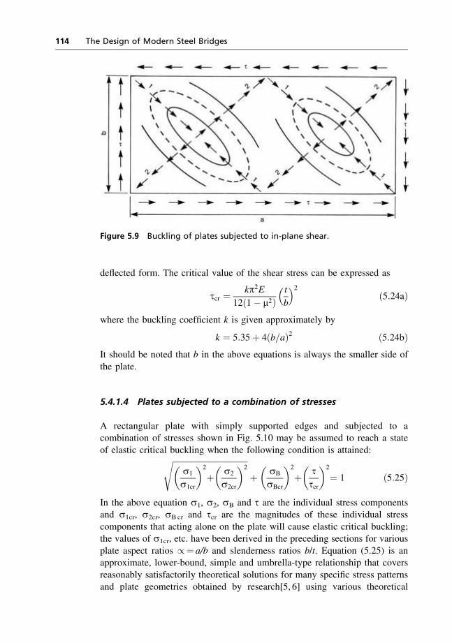
deflected form. The critical value of the shear stress can be expressed as

tcr ¼ kp2E12ð1� m2Þ

t

b

� 2ð5:24aÞ

where the buckling coefficient k is given approximately by

k ¼ 5:35þ 4ðb=aÞ2 ð5:24bÞIt should be noted that b in the above equations is always the smaller side of

the plate.

5.4.1.4 Plates subjected to a combination of stresses

A rectangular plate with simply supported edges and subjected to acombination of stresses shown in Fig. 5.10 may be assumed to reach a state

of elastic critical buckling when the following condition is attained:ffiffiffiffiffiffiffiffiffiffiffiffiffiffiffiffiffiffiffiffiffiffiffiffiffiffiffiffiffiffiffiffiffiffiffiffiffis1

s1cr

� �2

þ s2

s2cr

� �2s

þ sB

sBcr

� �2

þ ttcr

� �2

¼ 1 ð5:25Þ

In the above equation s1, s2, sB and t are the individual stress componentsand s1cr, s2cr, sBcr and tcr are the magnitudes of these individual stress

components that acting alone on the plate will cause elastic critical buckling;the values of s1cr, etc. have been derived in the preceding sections for various

plate aspect ratios /¼ a/b and slenderness ratios b/t. Equation (5.25) is anapproximate, lower-bound, simple and umbrella-type relationship that covers

reasonably satisfactorily theoretical solutions for many specific stress patternsand plate geometries obtained by research[5, 6] using various theoretical

Figure 5.9 Buckling of plates subjected to in-plane shear.


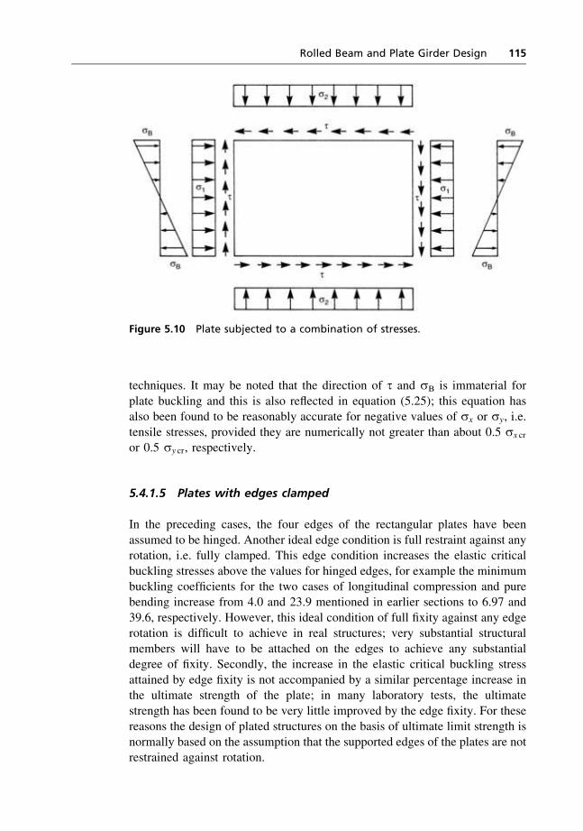
techniques. It may be noted that the direction of t and sB is immaterial for

plate buckling and this is also reflected in equation (5.25); this equation hasalso been found to be reasonably accurate for negative values of sx or sy, i.e.

tensile stresses, provided they are numerically not greater than about 0.5 sx cr

or 0.5 sy cr, respectively.

5.4.1.5 Plates with edges clamped

In the preceding cases, the four edges of the rectangular plates have been

assumed to be hinged. Another ideal edge condition is full restraint against anyrotation, i.e. fully clamped. This edge condition increases the elastic critical

buckling stresses above the values for hinged edges, for example the minimumbuckling coefficients for the two cases of longitudinal compression and purebending increase from 4.0 and 23.9 mentioned in earlier sections to 6.97 and

39.6, respectively. However, this ideal condition of full fixity against any edgerotation is difficult to achieve in real structures; very substantial structural

members will have to be attached on the edges to achieve any substantialdegree of fixity. Secondly, the increase in the elastic critical buckling stress

attained by edge fixity is not accompanied by a similar percentage increase inthe ultimate strength of the plate; in many laboratory tests, the ultimate

strength has been found to be very little improved by the edge fixity. For thesereasons the design of plated structures on the basis of ultimate limit strength is

normally based on the assumption that the supported edges of the plates are notrestrained against rotation.

Figure 5.10 Plate subjected to a combination of stresses.


5.4.2 Post-buckling behaviour of plates

In the preceding section the magnitude of the applied in-plane stress at whichan initially flat plate first buckles has been derived for various stress patterns.

Depending on the in-plane restraints on its edges, a buckled plate can carrystresses higher than this elastic critical stress, with the buckles growing in size

but still in a stable condition. If such stable buckles are acceptable, thenconsiderable gain in the strength of such plates is thus possible.

If the transverse edges of a rectangular initially flat plate approach eachother by a uniform amount across the width of the plate, then longitudinal

compressive stresses will also be uniform across the width, until the elasticcritical stress is reached and the plate buckles. After buckling, however, thecondition changes. Imagine the plate to be made up of a number of longitudinal

strips; the total distance by which the extremities of each longitudinal strip willapproach each other will be the sum of:

(1) the axial shortening of the strip due to the longitudinal compressive stresscarried by it, and

(2) the reduction in the chord length due to the bowing out-of-plane, or

buckling, of the strip.

It has been shown in the preceding section that a rectangular plate underlongitudinal compression buckles with only one half-wave across its width;

hence the longitudinal strip along the longitudinal centre line of the plate willbow out-of-plane, or buckle, by a bigger amount than the strips nearer the

longitudinal edges. If, after the onset of buckling, the transverse edges of thebuckled plate continue to approach each other by a uniform amount across

the width, it follows therefore that a central longitudinal strip will undergo lessaxial shortening and consequently carry lower longitudinal compressive stress,

than the strips nearer the longitudinal edges; this redistribution of the longi-tudinal stress, i.e. a transfer of stress from the relatively flexible central region

to the two regions near the longitudinal edges, is shown in Fig. 5.11.The conditions of in-plane restraint in the transverse direction along the two

longitudinal edges of the plate influence its post-buckling behaviour and stress

distribution. If these edges are free to move in-plane in the transverse direction,then stresses in the transverse direction are zero along these edges and are also

small in the interior of the plate; the longitudinal edges will, however, notremain straight but will pull in more in the crest and trough regions of the

buckles and less near the nodal lines. If the longitudinal edges are preventedagainst in-plane movement in the transverse direction, then significant

transverse tensile stresses develop; these will be higher in the crest and troughregions of the buckles and less near the nodal lines. An intermediate state oftransverse restraint along the longitudinal edges is when the edges are

constrained to remain straight though allowed to pull in, the net of averagetransverse stress along the edge being zero; in this case the transverse tensile


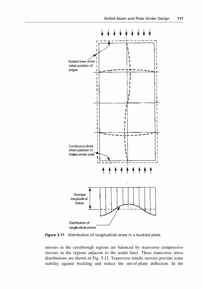
stresses in the crest/trough regions are balanced by transverse compressivestresses in the regions adjacent to the nodal lines. These transverse stress

distributions are shown in Fig. 5.12. Transverse tensile stresses provide somestability against buckling and reduce the out-of-plane deflection. In the

Figure 5.11 Distribution of longitudinal stress in a buckled plate.


post-buckling stage, the axial stiffness of the plate, i.e. the longitudinal

compressive force per unit area of cross-section divided by the longitudinalshortening per unit length, is given by:

(1) 0.75E, when the longitudinal edges are restrained against any pulling in(2) 0.5E, when the longitudinal edges are constrained to remain straight but

free to pull in(3) 0.41E, when the longitudinal edges are completely free to pull in.

These post-buckling stiffnesses are shown in Fig. 5.12(b). As the buckling of

the plate continues with increase in applied loading, the maximum longitudinalstress along the longitudinal edges reaches yield stress, or alternatively the

longitudinal stress along an interior longitudinal strip combined with flexuralstresses in the plate due to the buckles reaches the yield stress locally on the

Figure 5.12(a) Transverse stresses in buckled plates, with different longitudinaledge conditions. (i) Restrained against pulling in. (ii) Straight but free to pull in.(iii) Completely free to pull in.


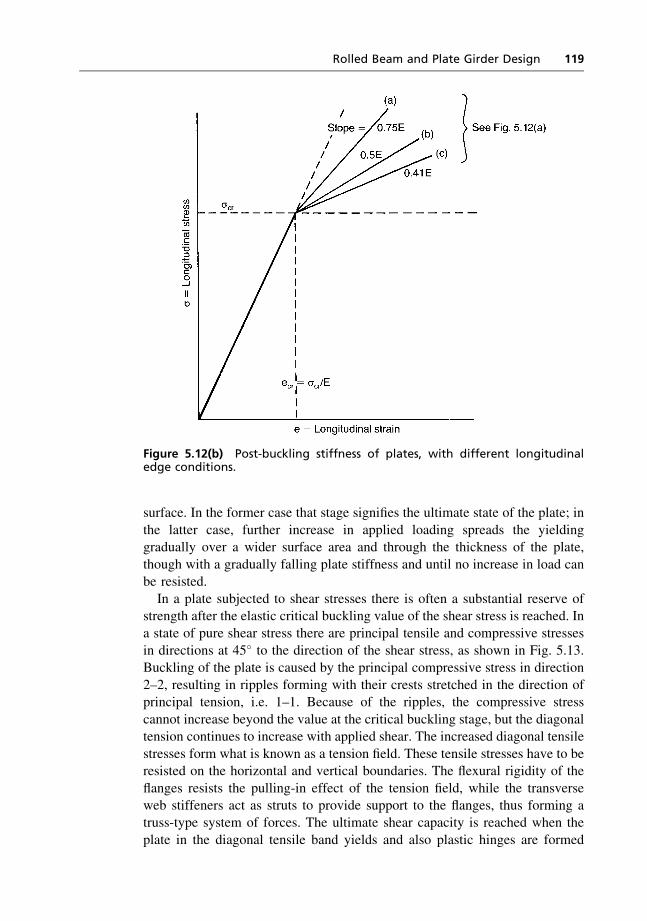
surface. In the former case that stage signifies the ultimate state of the plate; in

the latter case, further increase in applied loading spreads the yieldinggradually over a wider surface area and through the thickness of the plate,

though with a gradually falling plate stiffness and until no increase in load canbe resisted.

In a plate subjected to shear stresses there is often a substantial reserve ofstrength after the elastic critical buckling value of the shear stress is reached. Ina state of pure shear stress there are principal tensile and compressive stresses

in directions at 45� to the direction of the shear stress, as shown in Fig. 5.13.Buckling of the plate is caused by the principal compressive stress in direction

2–2, resulting in ripples forming with their crests stretched in the direction ofprincipal tension, i.e. 1–1. Because of the ripples, the compressive stress

cannot increase beyond the value at the critical buckling stage, but the diagonaltension continues to increase with applied shear. The increased diagonal tensile

stresses form what is known as a tension field. These tensile stresses have to beresisted on the horizontal and vertical boundaries. The flexural rigidity of the

flanges resists the pulling-in effect of the tension field, while the transverseweb stiffeners act as struts to provide support to the flanges, thus forming atruss-type system of forces. The ultimate shear capacity is reached when the

plate in the diagonal tensile band yields and also plastic hinges are formed

Figure 5.12(b) Post-buckling stiffness of plates, with different longitudinaledge conditions.


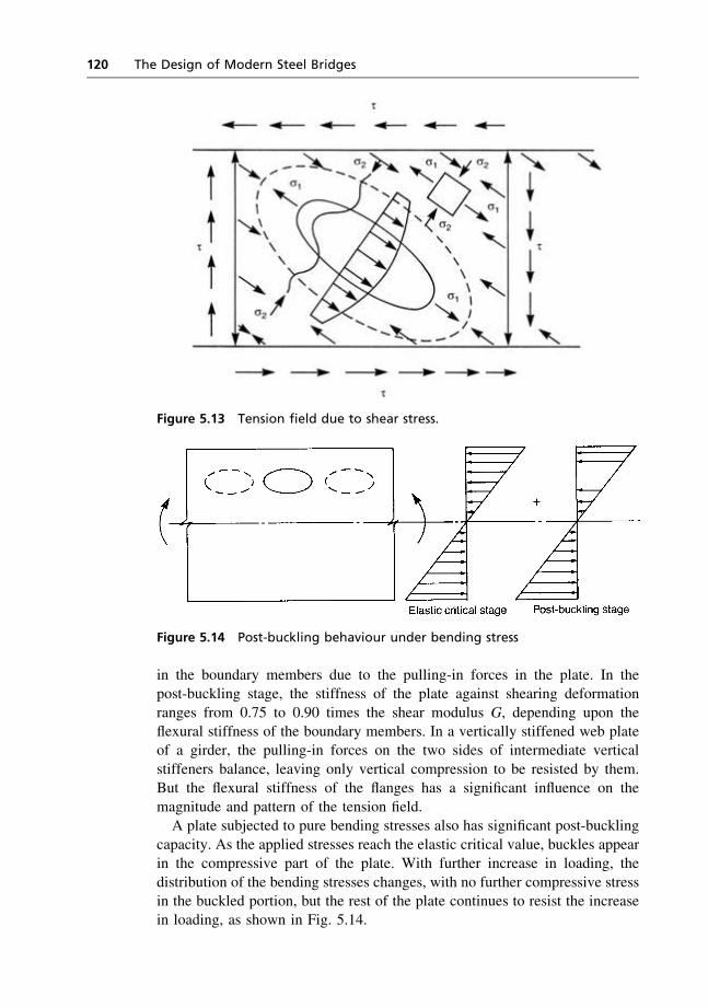
in the boundary members due to the pulling-in forces in the plate. In thepost-buckling stage, the stiffness of the plate against shearing deformation

ranges from 0.75 to 0.90 times the shear modulus G, depending upon theflexural stiffness of the boundary members. In a vertically stiffened web plateof a girder, the pulling-in forces on the two sides of intermediate vertical

stiffeners balance, leaving only vertical compression to be resisted by them.But the flexural stiffness of the flanges has a significant influence on the

magnitude and pattern of the tension field.A plate subjected to pure bending stresses also has significant post-buckling

capacity. As the applied stresses reach the elastic critical value, buckles appearin the compressive part of the plate. With further increase in loading, the

distribution of the bending stresses changes, with no further compressive stressin the buckled portion, but the rest of the plate continues to resist the increasein loading, as shown in Fig. 5.14.

Figure 5.13 Tension field due to shear stress.

Figure 5.14 Post-buckling behaviour under bending stress


5.4.3 Effect of residual stresses

Residual stresses in rolled steel sections are mainly caused by uneven coolingafter rolling; in sections fabricated by welding together several plates, the

residual stresses are caused by the shrinkage of the material in and adjacent tothe weld. In rolled I-sections, the flange tips cool first, but the delayed cooling

of the interior parts causes compressive stresses along the flange tips; thejunction between the flange and the web stays hot the longest and is thus

subjected to tensile stresses as the adjacent colder parts tend to prevent itsshrinkage. For equilibrium, the tensile and compressive longitudinal forces in

the cross-section must balance. A typical residual stress pattern in a rolledI-section is shown in Fig. 5.15. Compressive stress along the tip may be of theorder of 100–150N/mm2.

Welding or flame-cutting is associated with very high temperatures in alocalised strip. Shrinkage due to cooling of this strip is resisted by the

remaining cold portion of the steelwork. As a result, the strip adjacent to theweld or flame cut is subjected to high tensile strains which may be several

times the yield strain, and the rest of the steelwork is subjected to compression.A typical pattern is shown in Fig. 5.16. The shrinkage force due to welding can

be expressed as (CAw), where Aw is the cross-sectional area of the welddeposited and C is a constant dependent upon the welding process adopted.C has been found experimentally to vary from 7.5 to 12.5 kN/mm2; the lower

values in this range are typical of manual welding and the higher values areassociated with submerged arc welding. In multi-welds, if the steelwork is

allowed to cool down to room temperature between successive weld passes, Aw

is the area of weld deposited in one pass. A simplified pattern of the residual

stresses may be derived by assuming the tensile stresses in the strip adjacent tothe weld and the compressive stresses in the remaining area to be uniform in

their respective areas, and the former to be equal to the yield stress sy of the

Figure 5.15 Residual stresses in rolled sections.


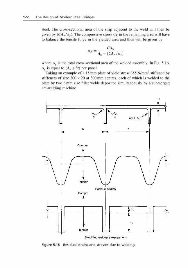
steel. The cross-sectional area of the strip adjacent to the weld will then be

given by (CAw/sy). The compressive stress sR in the remaining area will haveto balance the tensile force in the yielded area and thus will be given by

sR ¼ CAw

Ag � ðCAw=syÞ

where Ag is the total cross-sectional area of the welded assembly. In Fig. 5.16,Ag is equal to (ASþ bt) per panel.

Taking an example of a 15mm plate of yield stress 355N/mm2 stiffened bystiffeners of size 200� 20 at 300mm centres, each of which is welded to the

plate by two 6mm size fillet welds deposited simultaneously by a submergedarc-welding machine

Figure 5.16 Residual strains and stresses due to welding.


Aw ¼ 40mm2, allowing for a small concavity of the weld surface

CAw ¼ 12:5� 40 ¼ 500 kN

Ag ¼ 300� 15þ 200� 20 ¼ 8500mm2

sR ¼ 500 000

8500� ð500 000=355Þ ¼ 70:5N=mm2

As compressive and tensile residual stresses in the cross-section balance,residual stresses do not cause any resultant axial force or bending moment onany cross-section. If it is possible for the whole of the cross-section to squash,

i.e. yield in compression, then the axial load or bending moment capacity ofthe cross-section will be unaffected by residual stresses. However, those parts

of the cross-section where the residual stress is of the same nature as theapplied stress will reach yield stress earlier. For example, a welded box column

that can resist 300N/mm2 applied compressive stress in a residual-stress-freecondition may have some parts of its walls yielding at an applied stress level of

260N/mm2 if the welding compressive residual stress in the zone is 40N/mm2.For further applied loading these initially yielded parts of the cross-section willnot contribute any resistance and thus the effective stiffness of the cross-

section will fall. In the case of slender struts, the flexural rigidity of the cross-section is the most important parameter for their strength, and this is the reason

why residual stresses cause a reduction in their strength. The same applies tothat type of welded stiffened plate assembly where the buckling of the stiffener

out of the plane of the plate is more critical than the buckling of the platebetween the stiffeners.

For the strength of plate panels in compression the important question iswhether the plate panel, in a residual-stress-free condition, behaves in a stable

or unstable manner when the axial straining is continued after it reached itsmaximum capacity. This is illustrated in Fig. 5.17.In the case of plate (a), in the residual-stress-free condition the plate

continues to sustain the peak load su when further strained; the same platecross-section with welding residual compressive stress sR departs from its

initial primarily linear behaviour at an applied stress (su�sR), but withfurther applied strains reaches an ultimate load s0

u which is almost the same as

or just below su. In the case of plate (b), in the residual-stress-free conditionthe plate sheds off its axial load when the straining is continued beyond the

peak strength su; with residual stress the plate reaches a peak strength s0u

which is substantially below su. Stocky plates, i.e. with b/t ratios such that thecritical buckling stress scr is more than twice the yield stress sy, behave like

Fig. 5.17(a); so do very slender plates, i.e. those with critical buckling stressless than half the yield stress. But plates with intermediate slenderness, i.e.

with critical buckling stress between half and twice the yield stress, tend tobehave as in Fig. 5.17(b), and their strength is thus affected by the level of

welding compressive residual stress.


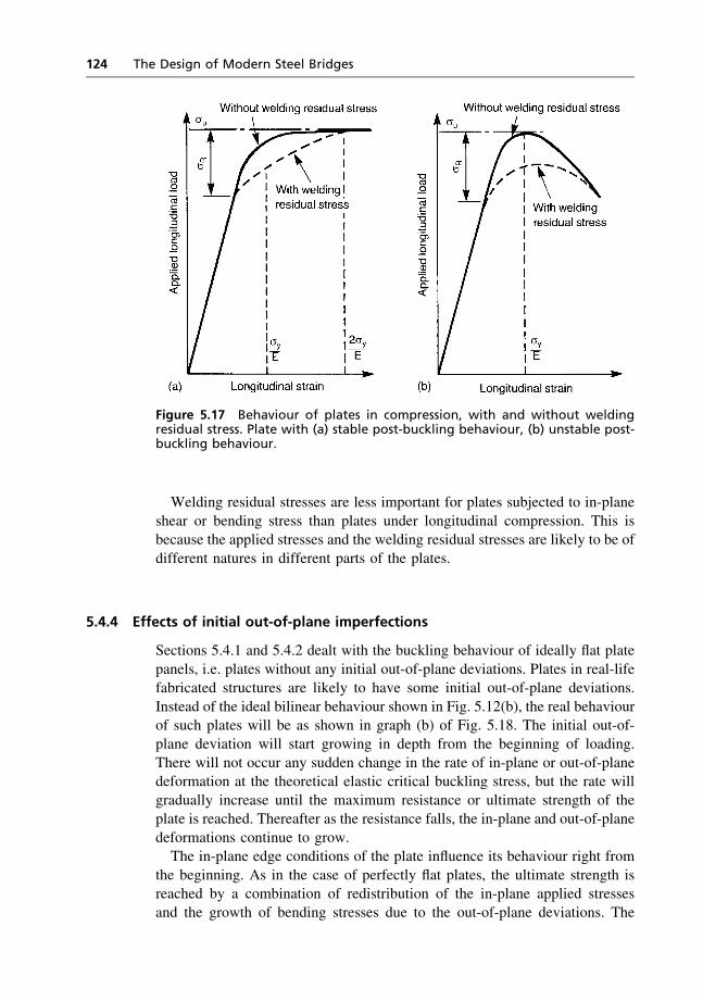
Welding residual stresses are less important for plates subjected to in-plane

shear or bending stress than plates under longitudinal compression. This isbecause the applied stresses and the welding residual stresses are likely to be of

different natures in different parts of the plates.

5.4.4 Effects of initial out-of-plane imperfections

Sections 5.4.1 and 5.4.2 dealt with the buckling behaviour of ideally flat plate

panels, i.e. plates without any initial out-of-plane deviations. Plates in real-lifefabricated structures are likely to have some initial out-of-plane deviations.

Instead of the ideal bilinear behaviour shown in Fig. 5.12(b), the real behaviourof such plates will be as shown in graph (b) of Fig. 5.18. The initial out-of-plane deviation will start growing in depth from the beginning of loading.

There will not occur any sudden change in the rate of in-plane or out-of-planedeformation at the theoretical elastic critical buckling stress, but the rate will

gradually increase until the maximum resistance or ultimate strength of theplate is reached. Thereafter as the resistance falls, the in-plane and out-of-plane

deformations continue to grow.The in-plane edge conditions of the plate influence its behaviour right from

the beginning. As in the case of perfectly flat plates, the ultimate strength isreached by a combination of redistribution of the in-plane applied stresses

and the growth of bending stresses due to the out-of-plane deviations. The

Figure 5.17 Behaviour of plates in compression, with and without weldingresidual stress. Plate with (a) stable post-buckling behaviour, (b) unstable post-buckling behaviour.


quantitative effects of initial out-of-plane deviations depend on:

(1) the magnitude of the deviations(2) the pattern of the deviations(3) the type of the applied stresses on the plate

(4) the in-plane and out-of-plane edge conditions of the plate(5) the slenderness (i.e. the width-to-thickness ratio) of the plate and to a

lesser extent its aspect ratio (i.e. the ratio of length to width).

Obviously, the larger the deviations, the worse are the effects. Initialdeviations in the pattern of the elastic critical buckling mode of the plate have

the worst effects. For example, in a plate with an aspect ratio of 3, subjected tocompression on the shorter edges, the worst pattern of initial deviations will bethe one with one sine wave across the width and three sine waves in the form

of ripples along the length. Plates subjected to in-plane compression along oneor both directions are most affected by initial deviations; plates in shear are

least affected. In-plane restraints on the edges reduce the effects of initialdeviations. But the beneficial effects of out-of-plane edge fixities (i.e. clamped

against rotation) are less pronounced in the case of initially curved plates thanthe improvement in the elastic critical buckling stress of a perfectly flat plate.

Plates with low slenderness, e.g. the width–thickness ratio less than, say, 20 inthe case of longitudinal in-plane compression or 50 in the case of in-plane

bending or shear, are able to reach their squash loading, i.e. applied stress canbe as high as the yield stress, in spite of any out-of-plane deviations. A more

Figure 5.18 Buckling behaviour of plates with initial out-of-plane deviations.(a) Ideally flat plate; (b) plate with initial out-of-plane deviations.


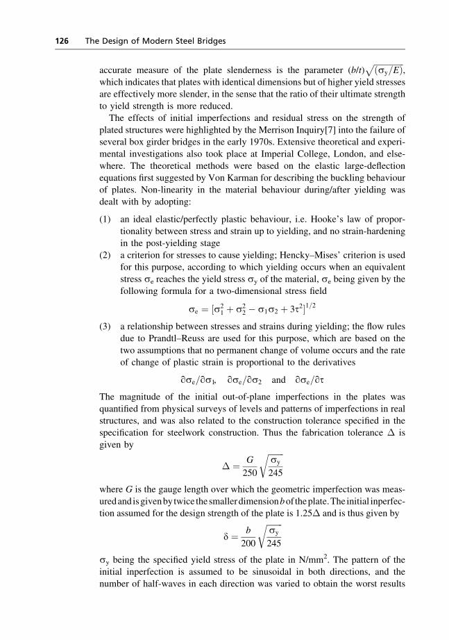
accurate measure of the plate slenderness is the parameter (b/t)ffiffiffiffiffiffiffiffiffiffiffiffiffiffiffiðsy=EÞ

p,

which indicates that plates with identical dimensions but of higher yield stressesare effectively more slender, in the sense that the ratio of their ultimate strength

to yield strength is more reduced.The effects of initial imperfections and residual stress on the strength of

plated structures were highlighted by the Merrison Inquiry[7] into the failure ofseveral box girder bridges in the early 1970s. Extensive theoretical and experi-

mental investigations also took place at Imperial College, London, and else-where. The theoretical methods were based on the elastic large-deflection

equations first suggested by Von Karman for describing the buckling behaviourof plates. Non-linearity in the material behaviour during/after yielding wasdealt with by adopting:

(1) an ideal elastic/perfectly plastic behaviour, i.e. Hooke’s law of propor-

tionality between stress and strain up to yielding, and no strain-hardeningin the post-yielding stage

(2) a criterion for stresses to cause yielding; Hencky–Mises’ criterion is usedfor this purpose, according to which yielding occurs when an equivalent

stress se reaches the yield stress sy of the material, se being given by thefollowing formula for a two-dimensional stress field

se ¼ ½s21 þ s2

2 � s1s2 þ 3t2�1=2

(3) a relationship between stresses and strains during yielding; the flow rulesdue to Prandtl–Reuss are used for this purpose, which are based on the

two assumptions that no permanent change of volume occurs and the rateof change of plastic strain is proportional to the derivatives

qse=qs1, qse=qs2 and qse=qt

The magnitude of the initial out-of-plane imperfections in the plates was

quantified from physical surveys of levels and patterns of imperfections in realstructures, and was also related to the construction tolerance specified in thespecification for steelwork construction. Thus the fabrication tolerance � is

given by

� ¼ G

250


245

r

where G is the gauge length over which the geometric imperfection was meas-

uredandisgivenbytwice thesmallerdimensionbof theplate.The initial inperfec-tion assumed for the design strength of the plate is 1.25� and is thus given by

d ¼ b

200


245

r

sy being the specified yield stress of the plate in N/mm2. The pattern of theinitial inperfection is assumed to be sinusoidal in both directions, and the

number of half-waves in each direction was varied to obtain the worst results


for the stress pattern under consideration. Generally this coincided with the

elastic critical buckling mode for the stress pattern. The main reason forrelating the imperfection to the yield stress sy was that the non-dimensional

imperfection parameter d/t could be related to the non-dimensional slendernessparameter (b/t)

ffiffiffiffiffiffiffiffiffiffiffiffiffiffiffiðsy=EÞp

as follows:

dt¼ 0:145

b

t

ffiffiffiffiffiffisy

E

r

and this allowed the non-dimensional strength parameters su/sy to be obtainedfrom the same strength graphs for all strength grades of steel. It was found thatplates subjected to in-plane shear or bending pattern of stresses were not very

sensitive to initial out-of-plane deviations, but plates subjected to in-planecompression were, and especially in the slenderness range of 40<

(b/t)ffiffiffiffiffiffiffiffiffiffiffiffiffiffiffiffiffiffiffiðsy=245Þ

p< 60. For example, in the above slenderness range, doubling

the initial imperfection amplitude from b/400 to b/200 or from b/200 to b/100

reduced the strength of the plate by up to 10%.Regarding initial welding residual stresses, it was found that both plates

under compression and plates under shear were sensitive, particularly in theslenderness range (b/t)

ffiffiffiffiffiffiffiffiffiffiffiffiffiffiffiffiffiffiffiðsy=245Þp

of 40 to 60 and 90 to 150, respectively,though by a lesser degree in the case of shear. For example, welding residual

compressive stress equal to 10% of the yield stress caused up to 10% reductionin the compressive strength of a plate with initial imperfection amplitude of

b/200, and an increase of welding compressive stress to 33% of the yield stresscaused another 10% reduction in the strength of that plate. A plate of

slenderness (b/t)ffiffiffiffiffiffiffiffiffiffiffiffiffiffiffiffiffiffiffiðsy=245Þ

p ¼ 120, and initial imperfection amplitude b/200had its shear strength reduced by 5% by welding compressive stress equal to

10% of the yield stress. Thus, even for plates that were sensitive to initialgeometric imperfections and welding residual stresses, assumptions of

(b/200)ffiffiffiffiffiffiffiffiffiffiffiffiffiffiffiffiffiffiffiðsy=245Þ

pand 0.1 sy for the two parameters yielded plate strengths

that were not substantially decreased with further increase in these twoparameters. Hence for design strength, the level of welding residual

compressive stress was assumed to be 10% of the yield stress.In these large-deflection elasto-plastic computer analyses, all four edges

were taken as simply supported, i.e. no restraint against rotation. The in-planeloading was applied as linear displacements of the edges, the resultant of the

edge stresses being taken as the applied edge load. In the case of pure in-planebending applied on the transverse edges, the longitudinal edges were held in

the shape of the simple bending curvature instead of being held straight.Plate strength curves are given in the British Standard BS 5400: Part 3 for

the two cases of:

(1) no in-plane restraint at the longitudinal edges, and

(2) longitudinal edges held straight (or in a pre-determined configuration, e.g.for pure bending case), but allowed to move inwards in-plane for the three


applied stress patterns of (i) uniaxial longitudinal compression, (ii) in-plane

shear, and (iii) in-plane pure bending. For a combination of these stresses,the interaction formula of equation (5.25) for elastic critical buckling was

found to produce results that were similar to those obtained from the large-deflection elasto-plastic computer analysis. In addition, a yielding check is

specified using the Hencky–Mises equation of

fs21 þ s2

2 � s1s2 þ 3t2g1=2>j sy

where s1 and s2 are stresses in two orthogonal directions and t is the shear

stress.

5.4.5 Tension field in girder webs

The preceding section dealt with the inelastic buckling strength of plate panelswith two types of in-plane restraints on edges. In the case of slender webs of

plate girders with transverse (i.e. vertical) stiffeners, the flanges usuallyconstitute an intermediate level of restraint between the two extremes of thelongitudinal edges being either fully free to pull in or fully held to remain

straight. The shear buckling strength of such webs can be obtained by ananalysis of the ‘tension field’ described in Section 5.4.2 and represented

pictorially in Fig. 5.13. As can be seen in this diagram, the diagonal stresses inthe web tend to pull the flanges inwards in the plane of the web. The relative

flexural rigidity of the flanges determines the amount they are pulled in, whichin turn determines the spread or width of the tension field. For example, with

very rigid flanges the tension field spreads uniformly over the whole panel; butwith very flexible flanges, the tension field band is narrow and is anchored

primarily from only the corners of the panel.The tension-field mechanism was first identified in plate girder railway

bridges towards the end of the nineteenth century. In the 1930s Wagner

developed a diagonal-tension theory for the web strength in aircraft fuselageson the assumption of negligible flexural rigidity of the web plate (i.e. the

elastic critical buckling strength equal to zero) and infinite flexural rigidity ofthe flanges in the plane of the web. According to this theory the ultimate

strength of the web in pure shear is given by sy/ffiffiffi2

pand is reached when the

diagonal tensile stress at 45� inclination to the horizontal boundaries

everywhere in the web panels attains the yield stress of the web material.Since then, many tension-field models have been proposed by theoretical andexperimental researchers. They are all based on the observation in tests that the

tensile membrane stress in the web, combining with the shear stress that ispresent prior to buckling, causes yielding of the web, and subsequent failure of

the whole panel is brought about by the formation of a mechanism involvingthe yielded zone of the web and plastic hinges in the flange.


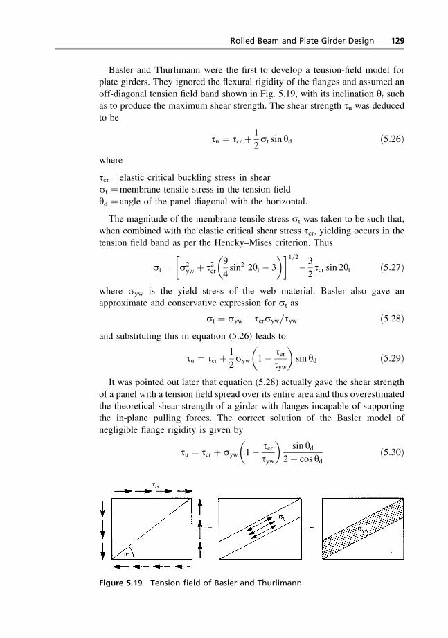
Basler and Thurlimann were the first to develop a tension-field model for

plate girders. They ignored the flexural rigidity of the flanges and assumed anoff-diagonal tension field band shown in Fig. 5.19, with its inclination yt suchas to produce the maximum shear strength. The shear strength tu was deducedto be

tu ¼ tcr þ 1

2st sin yd ð5:26Þ

where

tcr¼ elastic critical buckling stress in shear

st ¼membrane tensile stress in the tension fieldyd ¼ angle of the panel diagonal with the horizontal.

The magnitude of the membrane tensile stress st was taken to be such that,

when combined with the elastic critical shear stress tcr, yielding occurs in thetension field band as per the Hencky–Mises criterion. Thus

st ¼ s2yw þ t2cr

9

4sin2 2yt � 3

� �� 1=2� 3

2tcr sin 2yt ð5:27Þ

where syw is the yield stress of the web material. Basler also gave anapproximate and conservative expression for st as

st ¼ syw � tcrsyw=tyw ð5:28Þand substituting this in equation (5.26) leads to

tu ¼ tcr þ 1

2syw 1� ter

tyw

� �sin yd ð5:29Þ

It was pointed out later that equation (5.28) actually gave the shear strength

of a panel with a tension field spread over its entire area and thus overestimatedthe theoretical shear strength of a girder with flanges incapable of supportingthe in-plane pulling forces. The correct solution of the Basler model of

negligible flange rigidity is given by

tu ¼ tcr þ syw 1� tertyw

� �sin yd

2þ cos ydð5:30Þ

Figure 5.19 Tension field of Basler and Thurlimann.


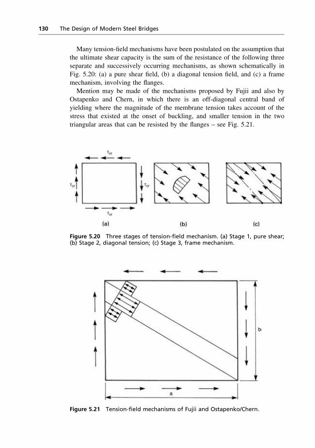
Many tension-field mechanisms have been postulated on the assumption that

the ultimate shear capacity is the sum of the resistance of the following threeseparate and successively occurring mechanisms, as shown schematically in

Fig. 5.20: (a) a pure shear field, (b) a diagonal tension field, and (c) a framemechanism, involving the flanges.

Mention may be made of the mechanisms proposed by Fujii and also byOstapenko and Chern, in which there is an off-diagonal central band of

yielding where the magnitude of the membrane tension takes account of thestress that existed at the onset of buckling, and smaller tension in the two

triangular areas that can be resisted by the flanges – see Fig. 5.21.

Figure 5.20 Three stages of tension-field mechanism. (a) Stage 1, pure shear;(b) Stage 2, diagonal tension; (c) Stage 3, frame mechanism.

Figure 5.21 Tension-field mechanisms of Fujii and Ostapenko/Chern.


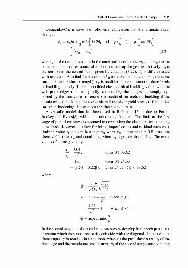
Ostapenko/Chern gave the following expression for the ultimate shear

strength

Vu ¼ tcrbt þ 1

2stbt sin 2yt � ð1� pÞ a

bþ ð1� pÞ a

bcos 2yt

h iþ 2

ampb þ mpt

� ð5:31Þ

where p is the ratio of tensions in the outer and inner bands, mpb and mpt are the

plastic moments of resistance of the bottom and top flanges, respectively, st isthe tension in the central band, given by equation (5.27). Vu is differentiatedwith respect to yt to find the maximum Vu (to avoid this the authors gave some

formulae for the shear strength). tcr is modified to take account of three levelsof buckling, namely (i) the unmodified elastic critical buckling value, with the

web panel edges rotationally fully restrained by the flanges but simply sup-ported by the transverse stiffeners, (ii) modified for inelastic buckling if the

elastic critical buckling stress exceeds half the shear yield stress, (iii) modifiedfor strain hardening if it exceeds the shear yield stress.

A versatile model that has been used in Reference [2] is due to Porter,Rockey and Evans[8], with some minor modifications. The limit of the first

stage of pure shear stress is assumed to occur when the elastic critical value tcris reached. However, to allow for initial imperfections and residual stresses, alimiting value tl is taken less than tcr when tcr is greater than 0.8 times the

shear yield stress ty, and equal to ty when tcr is greater than 1.5 ty. The exactvalues of tl are given by

t1ty

¼ 904

b2, when b533:62

¼ 1:0, when b524:55

¼ ð1:54� 0:22bÞ, when 24:55 < b < 33:62

where

b ¼ 1ffiffiffik

p b

tw

ffiffiffiffiffiffiffiffisyw

355

r

k ¼ 5:34þ 4

f2, when f51

¼ 5:34

f2þ 4, when f < 1

f ¼ aspect ratioa

b

In the second stage, tensile membrane stresses st develop in the web panel in adirection which does not necessarily coincide with the diagonal. The maximum

shear capacity is reached in stage three when (i) the pure shear stress tl of thefirst stage and the membrane tensile stress st of the second stage cause yielding


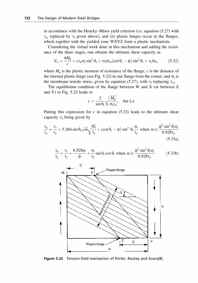
in accordance with the Hencky–Mises yield criterion (i.e. equation (5.27) with

tcr replaced by tl given above), and (ii) plastic hinges occur in the flanges,which together with the yielded zone WXYZ form a plastic mechanism.

Considering the virtual work done in this mechanism and adding the resist-ance of the three stages, one obtains the ultimate shear capacity as

Vu ¼ 4Mp

cþ ctwst sin

2 yt þ stbtwðcot yt � fÞ sin2 yt þ t1btw ð5:32Þ

where Mp is the plastic moment of resistance of the flange, c is the distance of

the internal plastic hinge (see Fig. 5.22) in one flange from the corner, and st isthe membrane tensile stress, given by equation (5.27), with tl replacing tcr.The equilibrium condition of the flange between W and X (or between Z

and Y) in Fig. 5.22 leads to

c ¼ 2

sin yt

ffiffiffiffiffiffiffiffiffiMp

sttw

r; but>j a

Putting this expression for c in equation (5.32) leads to the ultimate shear

capacity tu being given by

tuty

¼ t1ty

þ 5:264 sin ytffiffiffiffim

p ffiffiffiffiffist

ty

rþ ðcot yt � fÞ sin2 yt

st

tywhen m4

f2 sin2 ytst

6:928ty

ð5:33aÞ

tuty

¼ t1ty

þ 6:928m

fþ st

tysin yt cos yt when m5

f2 sin2 ytst

6:928tyð5:33bÞ

Figure 5.22 Tension-field mechanism of Porter, Rockey and Evans[8].


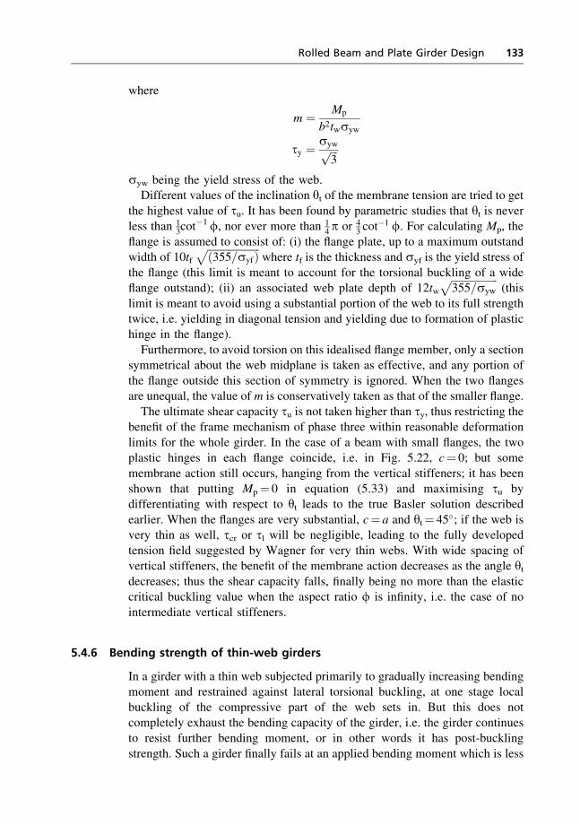
where

m ¼ Mp

b2twsyw

ty ¼ sywffiffiffi3

p

syw being the yield stress of the web.Different values of the inclination yt of the membrane tension are tried to get

the highest value of tu. It has been found by parametric studies that yt is neverless than 1

3cot�1f, nor ever more than 1

4p or 43 cot

�1 f. For calculating Mp, the

flange is assumed to consist of: (i) the flange plate, up to a maximum outstandwidth of 10tf

ffiffiffiffiffiffiffiffiffiffiffiffiffiffiffiffiffiffiffiffið355=syfÞp

where tf is the thickness and syf is the yield stress of

the flange (this limit is meant to account for the torsional buckling of a wideflange outstand); (ii) an associated web plate depth of 12tw

ffiffiffiffiffiffiffiffiffiffiffiffiffiffiffiffiffiffi355=syw

p(this

limit is meant to avoid using a substantial portion of the web to its full strengthtwice, i.e. yielding in diagonal tension and yielding due to formation of plastichinge in the flange).

Furthermore, to avoid torsion on this idealised flange member, only a sectionsymmetrical about the web midplane is taken as effective, and any portion of

the flange outside this section of symmetry is ignored. When the two flangesare unequal, the value of m is conservatively taken as that of the smaller flange.

The ultimate shear capacity tu is not taken higher than ty, thus restricting thebenefit of the frame mechanism of phase three within reasonable deformation

limits for the whole girder. In the case of a beam with small flanges, the twoplastic hinges in each flange coincide, i.e. in Fig. 5.22, c¼ 0; but some

membrane action still occurs, hanging from the vertical stiffeners; it has beenshown that putting Mp¼ 0 in equation (5.33) and maximising tu bydifferentiating with respect to yt leads to the true Basler solution described

earlier. When the flanges are very substantial, c¼ a and yt¼ 45�; if the web isvery thin as well, tcr or tl will be negligible, leading to the fully developed

tension field suggested by Wagner for very thin webs. With wide spacing ofvertical stiffeners, the benefit of the membrane action decreases as the angle ytdecreases; thus the shear capacity falls, finally being no more than the elasticcritical buckling value when the aspect ratio f is infinity, i.e. the case of no

intermediate vertical stiffeners.

5.4.6 Bending strength of thin-web girders

In a girder with a thin web subjected primarily to gradually increasing bendingmoment and restrained against lateral torsional buckling, at one stage localbuckling of the compressive part of the web sets in. But this does not

completely exhaust the bending capacity of the girder, i.e. the girder continuesto resist further bending moment, or in other words it has post-buckling

strength. Such a girder finally fails at an applied bending moment which is less


than its plastic moment of resistance. At this stage, the compressive part of theweb undergoes substantial buckling and consequently the compressive flange

buckles into the web as shown in Fig. 5.23.As a result of the buckling of the compressive part of the web, the distribution

of bending stress changes from the ideal linear pattern, as shown in Fig. 5.23,and the web becomes less efficient. To quantify the reduction in the bendingstrength of the web, the following reduction factor was suggested by Cooper[9]

for an I-beam of equal flanges and a web deeper than 5.7twffiffiffiffiffiffiffiffiffiffiffiffiffiE=syw

p1� 0:0005

Aw

Af

d

tw� 5:7

ffiffiffiffiffiffiffiffiE

syw

s !ð5:34Þ

where Aw and Af are the area of the web and each flange, respectively, and d isthe web depth. According to this approach there is no reduction in bending

strength if d=tw is less than 137 and 165 for syw¼ 355N/mm2 and 245N/mm2,respectively. Cooper’s expression for reduction in bending strength can also be

expressed as a reduced effective web thickness twe as follows:

twetw

¼ 1� d

tw� 5:7

ffiffiffiffiffiffiffiffiE

syw

s !0:003þ 0:0005

Aw

Af

� �ð5:35Þ

From the results of large-deflection elasto-plastic computer studies on thestrength of plate panels subjected to in-plane bending and with different edge

conditions, welding residual stresses and out-of-plane imperfections (seeSection 5.4.4), the following expression for the effective width is specified in

BS 5400: Part 3[2]

twetw

¼ 1:425� 0:00625dctw

ffiffiffiffiffiffiffiffisyw

355

rð5:36Þ

where dc is the depth of the compressive part of the web. This expression:

(1) ignores the effect of the different ratios of web to flange areas, as thiseffect, as predicted by equation (5.35), was in fact found to be quite small

(2) is valid for girders with equal or unequal flanges(3) stipulates no reduction in the effectiveness of the web if the ratio of the

depth of the compressive zone to thickness is less than 68 and 82 (or, in

Figure 5.23 Buckling of compressive part of web.


the case of equal flanges, the total web depth to its thickness ratio is less

than 136 and 164) for steel yield stresses of 355 and 245N/mm2, respectively.

These factors are marginally above the buckling coefficients discussed in

Section 5.4.4 for plate panels without any in-plane restraints at the edges andsubjected to applied in-plane bending stresses.

5.4.7 Combined bending moment and shear force on girders

Various researchers have extended their tension field models to apply to

coexistent shear force and bending moment on the girder sections. For example,in the tension field model due to Porter, Rockey and Evans[8], the elastic critical

stress can be reduced to take into account interaction with bending moment bymeans of a formula like equation (5.25), and the plastic moment of resistanceMp

of the flanges in equation (5.33) can be reduced by deducting the flange bendingstress from its yield stress. In Basler’s tension-field model, the shear is carried bythe web only, without any contribution from the flange; but this shear capacity is

only valid as long as themoment is less than the amount that can be resisted by theflanges only, i.e. less thansyfAfd. Any largermomentmust be resisted by bending

stresses in the webwhich reduces its shear capacity, until the latter becomes verysmall, possibly zero, when the bending moment reaches the full plastic moment

of the girder, or in the case of thin web girders its elastic moment of resistance.This interaction between moment and shear, in the absence of any lateral-

torsional or web buckling, can be represented by Fig. 5.24(a), where Vu

represents the full ultimate shear capacity of the girder and Vw represents the

value ignoring any contribution from the flange.In Reference [2] it has been assumed that, if the bending and shear capacities

are calculated without any contribution from the web and the flange, respec-

tively, then a beam can resist these values of bending moment M and shearforce V even when coexistent; this has been verified from many test results. Mf

is taken as sbAfd when sb is the limiting stress in the flange derived fromequation (5.13), Af is the flange area and d is the effective girder depth between

its flanges; Vw is obtained by putting Mp¼ 0 in equation (5.32) or (5.33). It hasbeen further assumed, supported by test results, that the bending capacityMu of

the girder as calculated for lateral-torsional buckling, elastic or plastic distri-bution of stresses or web buckling as appropriate, can be attained even whenthere is a coincident shear on the cross-section provided the latter is less than12Vw; similarly the full shear capacity Vu given by equation (5.33) is attainedeven in the presence of a coexistent bending moment provided the latter is less

than 12Mf. This interaction is shown in Fig. 5.24(b).

5.5 Design of stiffeners in plate girders

Stiffeners are often used to improve the buckling strength of plated structures.

Deflection of the plate normal to its plane along the line of stiffening is resisted


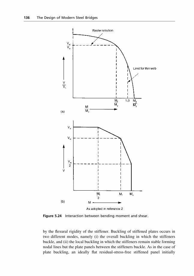
by the flexural rigidity of the stiffener. Buckling of stiffened plates occurs intwo different modes, namely (i) the overall buckling in which the stiffeners

buckle, and (ii) the local buckling in which the stiffeners remain stable formingnodal lines but the plate panels between the stiffeners buckle. As in the case of

plate buckling, an ideally flat residual-stress-free stiffened panel initially

Figure 5.24 Interaction between bending moment and shear.


remains flat until an elastic critical value of the loading is reached. Also, as in

the case of plates, stiffened plates may often have substantial post-bucklingstrengths.

5.5.1 Elastic critical buckling of stiffened panels

Two basic methods are available for the analysis of elastic critical buckling ofideally flat residual-stress-free stiffened plates. In the classical method, either

(i) a differential equation of equilibrium is solved in general terms by assuminga deflected shape and then the boundary conditions are used to obtain a

characteristic equation for the elastic critical buckling load, or (ii) a Fourier-type series representation is set up for the possible deformation mode consis-

tent with the boundary conditions and then an energy or work approach isapplied. The second method, i.e. the numerical or computer-based method, cantackle the complex problems; in this method a solution is formed in terms of a

discrete number of unknowns located at many points in the stiffened plate.Thus a large-order matrix equation is formed, whose coefficients are given by

the geometry of the stiffened plate and its loading conditions; the elasticcritical buckling load is the value of the load at which the determinant of the

coefficients is zero. The critical buckling load of a stiffened panel is generallyexpressed as

scr ¼ kp2Db2t

where k is a buckling coefficient that depends on the geometry of the stiffenedplate, the loading pattern and the boundary conditions, plus three relativerigidities of the stiffener, given by

� flexural: g ¼ EIs=bd

� torsional: y ¼ GJs=bd� extensional: d ¼ As=bt

and D is the flexural rigidity of the plate, equal to Et3=12ð1� m2Þb ¼ spacing of the stiffenerst ¼ thickness of the plateIs ¼ is the second moment of area of the stiffener cross-section, with the width

of the plate acting with it, about its centroidal plane parallel to the plateJs ¼ torsional constant of the stiffener cross-section

As ¼ area of the cross-section.

Many solutions are available for a large range of stiffened panel geometries

and loading types in References [10] and [11] for ‘open’-type stiffener cross-sections (i.e. not ‘closed’- or box-type cross-sections) with negligible torsional

rigidity.


5.5.2 The concept of optimum rigidity of stiffeners

If the buckling stress scr is plotted against the relative flexural rigidity g for astiffened plate with ‘open’-type stiffeners, it can be found that initially scr

increases with g; but after g exceeds a certain value g*, there is no furtherincrease in scr. For g< g* the buckling of the stiffened plate involves bending

of the stiffeners out of the plane of the plate as in mode (a) of Fig. 5.25, i.e. theoverall buckling mode; but for g> g* the plate panels between the stiffeners

and/or the boundaries buckle without any bending of the stiffeners, i.e. thestiffeners form the nodal lines of the buckling of the plate panels, as in mode

(b) of Fig. 5.25, i.e. local buckling of plate panels. There is thus an optimumrigidity g* of the stiffeners for the maximum possible value of the bucklingstress scr of the whole stiffened panel (i.e. for overall buckling), which

coincides with the elastic critical buckling stress of the individual plate panelsof the stiffened plate (i.e. for local buckling). No further increase in the

buckling load is possible by increasing g beyond this optimum value.The above concept of the optimum rigidity g* is thus based on the

fundamental concept of the elastic critical buckling phenomenon of both theentire stiffened panel and the individual plate panels in it. As has been pointed

out earlier, this concept is truly valid only for residual-stress-free perfectly flatplates with high yield stress; for a stiffened panel, in addition to thisrequirement the stiffeners must also be perfectly straight and residual-stress-

free. In reality, just as plates have residual stresses and out-of-plane imper-fections, so also the stiffeners have initial out-of-straightness and/or twist and

residual stresses. As a result stiffeners tend to deflect even at low levels ofapplied loading. In the overall buckling mode, i.e. g< g*, there is thus often nocritical value of loading at which sudden buckling of the stiffeners occurs.Instead, as the applied load is gradually increased, the deflection of the

stiffeners continues to increase at a gradually faster rate until no furtherincrease in load can be resisted. This maximum load is usually less than the

theoretical elastic critical value, but there are cases where, due to post-bucklingreserve, the maximum load is higher than the latter.In the local buckling mode, i.e. g> g*, because of their initial crookedness,

the stiffeners start deflecting even at low levels of loading and thus do not formnon-deflecting nodal lines for the local buckling of the individual plate panels;

as a consequence the elastic critical buckling load of the individual plate panelsis often not reached even when they have very low residual stress and out-of-

plane imperfections. The rigidity of the stiffeners has thus got to be n-times thetheoretical optimum value g* in order to ensure buckling in mode (b), i.e. local

buckling, of Fig. 5.25. The value of n depends upon the geometry of thestiffened panel and the type of loading and is found to vary from 2.5 to 5. Thus,according to the linear buckling theory of stiffened plates, either (i) stiffeners

are provided with n-times the optimum rigidity g* that will ensure that theoverall critical buckling stress is equal to the local critical buckling stress, or


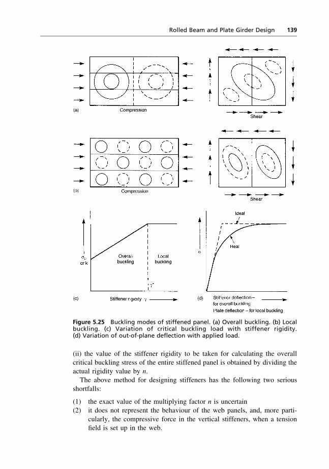
(ii) the value of the stiffener rigidity to be taken for calculating the overallcritical buckling stress of the entire stiffened panel is obtained by dividing the

actual rigidity value by n.The above method for designing stiffeners has the following two serious

shortfalls:

(1) the exact value of the multiplying factor n is uncertain(2) it does not represent the behaviour of the web panels, and, more parti-

cularly, the compressive force in the vertical stiffeners, when a tensionfield is set up in the web.

Figure 5.25 Buckling modes of stiffened panel. (a) Overall buckling. (b) Localbuckling. (c) Variation of critical buckling load with stiffener rigidity.(d) Variation of out-of-plane deflection with applied load.


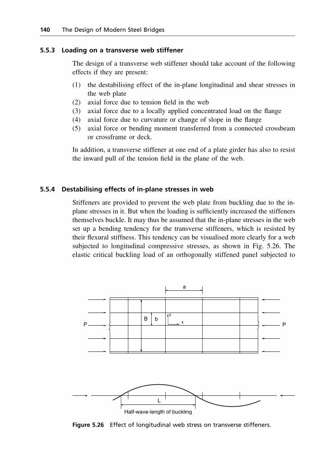
5.5.3 Loading on a transverse web stiffener

The design of a transverse web stiffener should take account of the followingeffects if they are present:

(1) the destabilising effect of the in-plane longitudinal and shear stresses in

the web plate(2) axial force due to tension field in the web

(3) axial force due to a locally applied concentrated load on the flange(4) axial force due to curvature or change of slope in the flange

(5) axial force or bending moment transferred from a connected crossbeamor crossframe or deck.

In addition, a transverse stiffener at one end of a plate girder has also to resistthe inward pull of the tension field in the plane of the web.

5.5.4 Destabilising effects of in-plane stresses in web

Stiffeners are provided to prevent the web plate from buckling due to the in-

plane stresses in it. But when the loading is sufficiently increased the stiffenersthemselves buckle. It may thus be assumed that the in-plane stresses in the webset up a bending tendency for the transverse stiffeners, which is resisted by

their flexural stiffness. This tendency can be visualised more clearly for a websubjected to longitudinal compressive stresses, as shown in Fig. 5.26. The

elastic critical buckling load of an orthogonally stiffened panel subjected to

a

B b

L

Half-wave-length of buckling

P P

y

x

Figure 5.26 Effect of longitudinal web stress on transverse stiffeners.


longitudinal compression is given by

Pcro ¼ p2

B

Dx

f2þ Dyf

2 þ 2H

� �

where Dx and Dy are the flexural rigidities in the orthogonal directions, H is the

torsional rigidity of the panel, and f is the aspect ratio L/B of the buckledpanel, L being the buckling half-wave-length in the x-direction.For minimum value of Pcro, the half-wave-length L¼B (Dx/Dy)

1/4 and the

minimum Pcro¼ 2p2/B [Dx �Dy)1/2þH].

For orthogonally stiffened web

Dx ¼ EIsx=b, and Dy ¼ EIsy=a

when Isx and Isy are the moments of inertia of the longitudinal and transversestiffeners, and b and a are their spacing respectively.

For torsionally weak stiffeners, i.e. stiffeners of open cross-section liketees, angles or flats, it is convenient and conservative to ignore the torsionalrigidity H. Hence

Pcro ¼ 2p2EB

IsxIsyab

� �1=2But if the critical half-wave-length L ¼ B ¼ fðIsx=bÞða=IsyÞg1=4 works out

less than a, then some half-waves will not contain a transverse stiffener andhence the above solution will not be valid. In that situation we should evaluate

Pcro by taking the lowest value for L that contain a transverse stiffener, i.e.L¼ a. This leads to

Pcro ¼ p2EB

Isx � B2

b � a2 þ Isy � a2a � B2

� �

As transverse stiffeners will be at the crest of the half-waves, their strainenergy will be double the strain energy of smeared stiffeners. Hence there is a

good case for doubling the second term in the bracket above.Let us denote

m ¼ Isx � ab � Isy

n ¼ a=B

Then

if m0:25 > n, Pcro ¼ p2EIsyB2

2m1=2

n

� �

and

if m0:25 < n, Pcro ¼ p2EIsyB2

mþ n4

n3

� �


For webs stiffened with vertical stiffeners only

Pcro ¼ 2p2

BðDx � DyÞ1=2, ignoring H

In this case Dx¼Et3/12[1� �2], and Dy¼EIsy/a, when t is the thickness of the

web and � is the Poisson’s ratio, equal to 0.3. Hence

Pcro ¼ 6E

B

t3 � Isya

� �1=2

We may design a transverse stiffener as a strut with an effective axial load

Peq such that the ratio of this effective axial load to the Euler buckling load ofthe strut, PE, is equal to the ratio of the longitudinal force on the web to theorthotropic elastic critical buckling load Pcro derived from above, i.e.

Peq

PE¼ s1tB

Pcro

wherefrom

Peq ¼ s1tBPE

Pcro

We should also take account of the fact that the destabilising forces in theweb do not cause any axial stress on the transverse stiffeners. If a strut with an

initial imperfection �i is subjected to a destabilising force Peq that magnifiesthe initial imperfection, but does not cause any axial stress, the limiting value

Peql of this force that will initiate yielding on an extreme fibre will be given by

Peq1 ��iPE

PE � Peq1� y

Ar2¼ sy

which leads to

Peq1 ¼ Py

Zþ Py

PE

where

Z ¼ �iy

r2

r ¼ radius of gyration

y ¼ extreme compressive fibre distance

A ¼ cross-sectional area

Py ¼ squash load ¼ syA:

Peql will obviously be greater than the strut strength Ps of a normal axiallyloaded strut with initial imperfections �i. We can thus apply a reduction factorPs/Peql to evaluate Peq on the transverse stiffener, thus leading to


Peq ¼ s1tB � PE � Ps

Pcro � Peq1

¼ s1tBPE

Pcroð2:5ksÞ ð5:37Þ

where

ks ¼ 4Ps

p2PyZþ Py

PE

� �

Using the expressions for Pcro derived earlier, we have:

(1) for webs stiffened longitudinally and vertically

ðaÞ if m0:25 > n

Peq ¼ s1tBn

2m1=2� ð2:5ksÞ ¼ 1:25s1tBksnm

�1=2 ð5:38Þ

ðbÞ if m0:25 < n

Peq ¼ s1tBn3

mþ n4ð2:5ksÞ ¼ 2:5s1tBks

n3

mþ n4ð5:39Þ

(2) for webs with transverse stiffeners only

Peq ¼ s1tBp2EIsyB2

B

6E

a

t3Isy

� �1=2� ð2:5ksÞ

¼ 4:1s1ksaIsyt

� �1=2ð5:40Þ

In the first edition of this book, the critical buckling load of a transversely

stiffened web was derived from an assumed buckling mode of saw-toothpattern, consisting of straight longitudinal strips of web between transverse

stiffeners and the latter deflecting alternately inwards and outwards. The criticalbuckling load Pcro was derived from this buckling mode as

p4EIsya4B3

This expression would predict that Pcro would increase with any increase inthe spacing a of the transverse stiffeners, all other parameters remaining the

same. This is obviously unrealistic. The assumed saw-tooth buckling mode isreally invalid, as the straight longitudinal strips are assumed to be of negligibleflexural stiffness and would thus be unable to resist any applied longitudinal

compressive loading.A study of the elastic critical buckling solutions for many stiffened panel

geometries in References [10] and [11] indicates that the magnitude of thecritical shear stress of the panels is numerically very similar to the critical

longitudinal compressive stress. Thus, sl above can be taken as the sum of the


shear stress and the longitudinal stress in the web. When the distribution of

longitudinal stress in the web is not purely uniform compression, but acombination of uniform compression sl and pure in-plane longitudinal bending

sb, such that sl�sb give the stresses at the edges of the web (see Fig. 5.10),then (sIþ1

6 sb) may be taken instead of sl only in equations (5.38)–(5.40); this

is based on the observation that the elastic critical buckling coefficient k is 4for pure compression and 24 for pure bending (see Section 5.4.1).

5.5.5 Axial compression due to tension field in web

The tension field in the web constitutes diagonal tensile stresses in it, the

vertical component of which has to be resisted by vertical web stiffeners. Thisis very like the force distribution in an N-type truss and is shown in Fig. 5.27.

In Section 5.4.5 it has been postulated that when the applied shear stressexceeds the elastic critical value, the rest of the shear stress is resisted by the

tension field mechanism. Under the combined action of shear and bendingstresses in the web, elastic critical buckling occurs when the following condi-tion is reached (see Section 5.4.1.4)

s1

s1crþ sB

sBcr

� �2

þ ttcr

� �2

¼ 1 ð5:41Þ

where

sl ¼ uniform longitudinal compressive stress in web

sB¼ pure longitudinal bending stress in webt ¼ shear stress in web

s1cr ¼ 4p2E12ð1� m2Þ

twb

� 2

sBcr ¼ 24p2E12ð1� m2Þ

twb

� 2

tcr ¼ kp2E12ð1� m2Þ

twb

� 2

k ¼ 5:35þ 4b

a

� �2

9>>>>>>>>>>>>>>=>>>>>>>>>>>>>>;

(see Section 5 :4.1)

Because of imperfections and residual stresses in the web, it may be conser-vatively assumed that tension field action starts when the applied stresses

exceed 80% of the elastic critical buckling values, i.e. slcr, sBcr and tcr aboveare reduced by multiplying by 0.8.

A further simplifying and conservative step will be to assume the power ofthe second term in equation (5.41) to be 1, instead of 2. This will then lead to


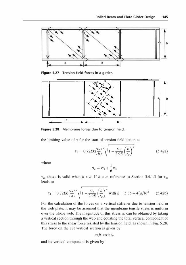
the limiting value of t for the start of tension field action as

t1 ¼ 0:72Ektwb

� 2 ffiffiffiffiffiffiffiffiffiffiffiffiffiffiffiffiffiffiffiffiffiffiffiffiffiffiffiffiffiffiffiffi1� sc

2:9E

b

tw

� �2s

ð5:42aÞ

where

sc ¼ s1 þ 1

6sB

tcr above is valid when b < a. If b > a, reference to Section 5.4.1.3 for tcrleads to

t1 ¼ 0:72Ektwa

� 2 ffiffiffiffiffiffiffiffiffiffiffiffiffiffiffiffiffiffiffiffiffiffiffiffiffiffiffiffiffiffiffiffi1� se

2:9E

b

tw

� �2s

with k ¼ 5:35þ 4ða=bÞ2 ð5:42bÞ

For the calculation of the forces on a vertical stiffener due to tension field inthe web plate, it may be assumed that the membrane tensile stress is uniform

over the whole web. The magnitude of this stress st can be obtained by takinga vertical section through the web and equating the total vertical component of

this stress to the shear force resisted by the tension field, as shown in Fig. 5.28.The force on the cut vertical section is given by

stb cos yttw

and its vertical component is given by

Figure 5.28 Membrane forces due to tension field.

Figure 5.27 Tension-field forces in a girder.


ðstb cos yttwÞsin ytThe shear force resisted by tension field action is

ðt� t1ÞbtwEquating

st ¼ ðt� t1Þsin yt cos yt

ð5:43Þ

Due to st, the pull on the flanges per unit length is

sttw sin yt

and its vertical component is

sttw sin2 yt

The compressive force Ptf on a vertical stiffener is equal to the vertical compon-ent of the total pull over length a on the flanges. Thus

Ptf ¼ statw sin2 yt

¼ t� t1sin yt cos yt

atw sin2 yt, using equation (5:43)

¼ ðt� t1Þatw tan yt

ð5:44Þ

The inclination of the membrane forces yt for the maximum shear resistancedue to tension-field action has been found from parametric studies never to

exceed p/4, nor does it exceed the angle of the diagonal of the web panel withthe horizontal for aspect ratio a/b of the panel up to 3. Hence Ptf can be taken as

Ptf ¼ ðt� t1Þatw, or ðt� t1Þbtwwhichever is smaller.

Due to st, the pull on an end vertical stiffener per unit height is

sttw cos yt

and its horizontal component is

sttw cos2 yt

Assuming some end fixity, the bending moment on an end post is

sttw cos2 ytb2

10¼ 1

10ðt� t1Þtwb2 cot yt

from equation (5.43).

From parametric studies for the maximum shear resistance due to tension-field action, an upper band for cot yt was found to be 80/yd, where yd is the

inclination of the diagonal of the web panel with the horizontal in degrees. Thedesign bending moment My on an end stiffener can thus be expressed as

My ¼ 8ðt� t1Þtwb2=yd


5.5.6 Design of longitudinal web stiffeners

The critical buckling load of a longitudinally loaded orthogonally stiffened webhas been derived in Section 5.5.4 as

Pcro ¼ 2p2EB

Isx � Isya � b

� �1=2with the notations as in that section.

For a particular ratio of the moments of inertia of the transverse andlongitudinal stiffeners Isy and Isx, see Figure 5.26, Pcro will be equal to the sum

of the Euler buckling loads of the longitudinal stiffeners, i.e. when

2p2EB

Isx � Isya � b

� �1=2¼ p2E

Isxa2

B

b� 1

� �

or

Isy ¼ 1

4

IsxbB2

a3B

b� 1

� �2With this value of Isy, the half-wave-length L will be

B � Isx � ab � Isy

� �1=4¼

ffiffiffi2

pa

B

B� b

� �1=2If Isy is greater than the above value, the sum of the Euler buckling loads will

be less than Pcro; there is also the possibility that there may not be a transversestiffener within the half-wave-length L, thus invalidating the evaluation of Pcro

as above. Hence in this situation the longitudinal stiffeners should be designed

as struts with effective length equal to a.If Isy is less than the above value, the orthotropic critical buckling load Pcro

will be less than the sum of the Euler buckling loads of the longitudinalstiffeners. Hence the longitudinal stiffeners should be designed as struts with

effective length leff greater than a and given by

p2EIsxl2eff

B

b� 1

� �¼ 2p2E

B

Isx � Isya � b

� �1=2

wherefrom

leff ¼ B

2

B

b� 1

� �� 1=2� abIsx

Isy

� �1=4The axial loading on a longitudinal stiffener should include not only the

longitudinal stresses in the girder web, but should also allow for the destabi-lising effects of shear stresses and any transverse stresses in the web. Thus the

applied longitudinal stress should be taken as

s1 þ 2:5ksðtþ s2Þ


where

s1¼ applied longitudinal stress on the stiffener

t ¼ shear stress in the webs2¼ transverse stress in the web

ks ¼ defined in Section 5.5.4.

5.6 Restraint at supports

The lateral buckling strength of beams has been derived in Section 5.3 on theassumption that its cross-section at the supports is restrained fully against any

lateral deflection of its flanges. In reality the stiffeners at the support restraintto prevent twisting of the beam section is likely to be finite. Flint[12] has

derived a reduction in the elastic critical bending strength scr of a perfectsimply supported beam as

�scr

scr¼ 4

3

GJ

LeSfor a central concentrated load

¼ 2GJ

LeS

for constant bending moment on the

whole length of the beam:

where

GJ¼ torsional rigidity of the beamLe ¼ effective length of the beam

S ¼ stiffness of the support against twisting of the beam section.

The reduction �sb in the limiting bending stress sb of the imperfect simplysupported beam is, taking the worse of the above two cases

�sb

sb¼ �scr

scr

�sb

�scr

scr

sb¼ 2GJ

LeS

�sb

�scr

scr

sb

If we decide to limit �sb to n% of sb, then

2GJ

LeS� �sb

�scr

scr

sb4 0:01 � n

or

S5200

n

GJ

Le

�sb

�scr

scr

sbð5:45Þ

From equations (5.7) and (5.8) in Section 5.3.1, assuming k, � and the shapefactor (i.e. the ratio of the plastic to elastic modulus) to be each approximately

equal to unity, scr can be expressed as

scr

sy¼ p2

Lery


E

r� ��2

¼ 5700

b2


when

Le is the effective length for lateral torisional buckling of the beamry is the radius of gyration of the beam cross-section about the y–y axis

b ¼ Lery


355

r

The ratio sb=sy is equal to the ratio MR=MU for which an expression wasderived in equation (5.13) of Section 5.3.2; thus

sb

sy¼ MR

MU¼ 1

21þ ð1þ ZÞ 5700

b2

� �� 1

21þ ð1þ ZÞ 5700

b2

� �2

� 22 800

b2

" #1=2

where

Z ¼ 0:008ðb� 30Þ for beams fabricated by longitudinal welding

¼ 0:0035ðb� 30Þ for other beams.

From the above two expressions for scr/sy and sb/sy, the product of(�sb /�scr)(scr /sb) has been found conservatively given by 0.0075b. Hence

S5200

n� GJLe

� ð0:0075ÞLery


355

r

i.e.

51:5

n

GJ

ry


355

r

If 1% fall in the allowable bending stress sb is acceptable, then the stiffnessof the torsional restraint at support should not be less than

1:5 � GJry

�ffiffiffiffiffiffiffiffisy

355

r

When the torsional restraint at the support section of a simply supportedI-beam consists only of a load-bearing stiffener anchored to the pier or the

abutment, the actual stiffness of the restraint is equal to

3EIsD

where Is is the second moment of area of the cross-section of the load-bearing

stiffener about a horizontal axis along the web of the beam.

5.7 In-plane restraint at flanges

In Section 5.4.4 it was stated that the behaviour and strength of an initiallyimperfect plate subject to in-plane loading depended upon the degree of in-

plane restraint on the edges. In British Standard BS 5400: Part 3[2] separate


graphs are given for the strength of:

(1) plates without any in-plane restraint on the longitudinal edges, i.e. free to

pull in(2) plates with longitudinal edges constrained to remain straight but allowed

to move inwards in the plane.

Any in-plane restraint on the horizontal edges of an external web panel willapply a distributed load on the flange of a beam in the plane of the web;similarly, vertical edges at the ends of a beam will be subjected to in-plane

pulling-in forces for which a vertical stiffener over an external support needs tobe designed. Along the internal edges of web plate panels the pulling-in forces

in adjacent panels will tend to balance, and hence such edges may be deemedto remain virtually straight. For plates subjected to shear, its strength in the

tension field mechanism depends upon the bending capacity of the flange (seeSection 5.4.5). For plates subject to any pattern of in-plane loading, it is

necessary to establish some criteria as to when the edges adjacent to a flangemay be assumed to remain straight.

5.7.1 Plates under compression

For a plate panel under longitudinal compression s1, with initial imperfectionsin the critical buckling mode and with longitudinal edges held straight but free

to pull in, the author has derived[14] the following expression for the trans-verse in-plane stresses at the longitudinal edges

s2 ¼ p2

8ðm2 � 1Þ d

2E

b2cos

2pNxL

ð5:46Þ

where

L ¼ length of the plate in the longitudinal direction xx ¼ longitudinal distance from the transverse centre line

N¼ number of half-waves in direction x (�L/b)b ¼width of the plate

d ¼ amplitude of the initial imperfectionm¼ factor of magnification of initial imperfections under the loading sl

E ¼Young’s modulus.

From the above expression, the maximum amplitude of s2 can be expressed as

s2

sy¼ p3

8ðm2 � 1Þ d0

S

� �2

ð5:47Þ

where

d0¼ a non-dimensional imperfection parameter d/tt ¼ plate thickness


S ¼ a non-dimensional slenderness parameter (b/t)ffiffiffiffiffiffiffiffiffiffiffiffiffiffiffiðsy=EÞ

psy¼ yield stress of the plate.

The author has also shown[14] that the value of m that is reached when theapplied stress s1 reaches the ultimate strength of the panel is given by

0:7d20m2 � 1

m¼ 0:2766S2 þ 0:7d20 � 1 ð5:48Þ

In Section 5.4.4 it was stated that, on the basis of the specified tolerances onworkmanship, d0 can be assumed as 0.145S. For any particular value of S, d0can thus be quantified, and then from equation (5.48) the value of m may beobtained by successive approximation. The amplitude of the cosine distribution

for s2/sy can then be obtained from equation (5.47). By this procedure a graphfor s2/sy against slenderness parameter S was drawn. It was found that s2/sy

could be taken as:

(1) zero, up to S¼ 1.0

(2) 0.5, for S> 3.6(3) 0.192 (S� 1), for 1.0< S< 3.6.

The cosine distribution of s2 on the edge, given by equation (5.46), causes

a bending moment distribution on the girder flange on the edge, given by

M ¼ b2

4p2s2t

The moment of resistance of the flange section MR has to be at least a safety

factor times the maximum value of the above bending moment. Taking accountof the longitudinal stress already present in the flange due to the bending

moment on the girder, the plastic moment of resistance MR can be taken as

MR ¼ 1

4syfBT

2f 1� sf

syf

� �2" #

where

B ¼width of the flangeTf ¼ thickness of the flange

sf ¼ longitudinal stress in the flangesyf¼ yield stress of the flange.

Assuming a safety factor of 1.25

MR51:25M

or

1

4syfBT

2f 1� sf

syf

� �2" #

51:25b2

4p2s2t


or

syfBT2f

syb2t5

1:25

p2s2

sy

s2yf

s2yf � s2

f

!

For S4 1.0, s2 is zero and hence any web panel adjacent to a flange and withslenderness ratio S4 1.0 may be taken as restrained irrespective of the size of

the girder flange. For web panels with S5 3.6, s2¼ 0.5 sy, and hence such apanel adjacent to a flange can be considered restrained only if the following

condition is satisfied for the size of the flange

syfBT2f

syb2t50:0625

s2yf

s2yf � s2

f

!ð5:49Þ

For a web panel adjacent to a flange and with slenderness ratio 1.0< S< 3.6,the flange size has to satisfy the following condition for the panel to beconsidered restrained

syfBT2f

syb2t5

1:25

p20:192ðS� 1Þ s2

yf

s2yf � s2

f

!

i.e.

5 0:024ðS� 1Þ s2yf

s2yf � s2

f

!ð5:50Þ

5.7.2 Plates under shear

In Section 5.4.5 the tension-field strength of a plate subjected to shear wasshown to depend upon a flange stiffness parameter m given by

m ¼ Mp

b2tsy

This parameter is one-quarter of the ratio of the plastic moduli of the flangeplate and the web plate about their respective horizontal centroidal axes, whichhas been used in the section above for determining the flange stiffness required

to achieve restrained plate capacity under compressive applied loading. Theminimum values of m required to achieve in the tension field mechanism the

levels of shear capacities represented by the restrained plate capacities in shearmay be obtained from the expression for tension field strength for different

aspect ratios of the plate. These minimum values should, however, be increasedby a safety margin, since the tension field mechanism is attained with defor-

mations in the plate, and in the flange member, of a much larger magnitudethan is associated with the ultimate strength of orthogonally stiffened plates.By this method, the following stiffness requirement for the flange member has


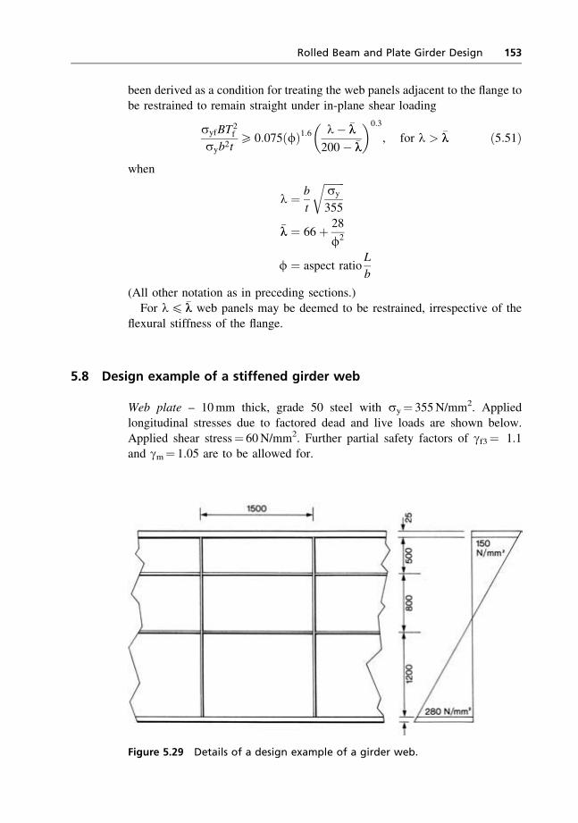
been derived as a condition for treating the web panels adjacent to the flange to

be restrained to remain straight under in-plane shear loading

syfBT2f

syb2t5 0:075ðfÞ1:6 l� �ll

200� �ll

� �0:3

, for l > �ll ð5:51Þ

when

l ¼ b

t


355

r

�ll ¼ 66þ 28

f2

f ¼ aspect ratioL

b

(All other notation as in preceding sections.)

For l4 �ll web panels may be deemed to be restrained, irrespective of theflexural stiffness of the flange.

5.8 Design example of a stiffened girder web

Web plate – 10mm thick, grade 50 steel with sy¼ 355N/mm2. Appliedlongitudinal stresses due to factored dead and live loads are shown below.

Applied shear stress¼ 60N/mm2. Further partial safety factors of gf3¼ 1.1and gm¼ 1.05 are to be allowed for.

Figure 5.29 Details of a design example of a girder web.


Yielding check – Hencky–Mises equivalent stress at top edge:

se ¼ f1502 þ 3� 602g0:5 ¼ 182:5N=mm2

Reference [2] allows for some plastic redistribution of the bendingcomponent of the longitudinal stress by taking only 0.77 times the bending

stress. The top panel is subjected to 107N/mm2 direct compression and 43N/mm2 bending stress. Hence

se ¼ fð107þ 0:77� 43Þ2 þ 3� 602g0:5 ¼ 176:4N=mm2

Bottom edge:

se ¼ f2802 þ 3� 602g0:5 ¼ 298:7N=mm2

With plastic redistribution of bending stress in bottom panel

se ¼ fð176:8þ 0:77� 103:2Þ2 þ 3� 602g0:5 ¼ 276:5N=mm2

Limiting value of

se ¼ 355=ð1:1� 1:05Þ ¼ 307:4N=mm2

Hence the design is satisfactory for yielding.

Buckling check

(1) Top panel: to check if the panel can be deemed restrained for compress-ive and shear stresses. To take compression first

BT2f

b2t¼ 500� 252

5002 � 10¼ 0:125

which is greater than the minimum required as calculated below

sf ¼ 152:15� 1:1� 1:05 ¼ 175:7N=mm2

S ¼ b

t


E

r¼ 50

ffiffiffiffiffiffiffiffiffiffiffiffiffiffiffiffi355

205 000

r¼ 2:08

0:024ðS� 1Þfs2yf=ðs2

yf � s2f Þg ¼ 0:024� 1:08� 1:325 ¼ 0:0343

For shear, also, the slenderness ratio is such that the plate can be taken asrestrained.The panel is subjected to 107N/mm2 compressive, 43N/mm2 bending and

60N/mm2 shear stresses. Buckling stress coefficients are obtained fromReference [2] for

b

t


355

r¼ 50 and f ¼ 3

as follows:

K1 ¼ coefficient for axial compression¼ 0.675

Kb ¼ coefficient for pure bending¼ 1.205(a value higher than 1.0 recognises plastic redistribution of bendingstress at ultimate state)

Kq ¼ coefficient for shear¼ 0.966.


For interaction of various stress components the following ratios are calculated:

mc ¼ s1gmgf3syK1

¼ 107� 1:05� 1:1

355� 0:675¼ 0:516

mb ¼ sbgmgf3syKb

� �2

¼ 43� 1:05� 1:1

355� 1:205

� �2

¼ 0:013

mq ¼ tgmgf3syKq

� �2

¼ 60� 1:05� 1:1

355� 0:966

� �2

¼ 0:041

mc þ mb þ 3mq ¼ 0:652 < 1:00

Hence the panel is safe for buckling.

(2) Middle panel: this panel is subjected to 4.8N/mm2 tensile, 68.8N/mm2

bending and 60N/mm2 shear stresses. Being an internal panel, it is deemed tobe restrained.

Buckling stress coefficients are obtained from Reference [2] for

b

t


355

r¼ 80, and f ¼ 150

80¼ 1:875

as follows:

K1 ¼ 48

Kb ¼ 1:15; interpolating between f ¼ 1 and 2

Kq ¼ 0:939

mc ¼ 4:8� 1:1� 1:05

355� 0:48

mb ¼ 68:8� 1:1� 1:05

355� 1:15

� �2

mq ¼ 60� 1:1� 1:05

355� 0:939

� �2

mc þ mb þ 3mq << 1:00


(3)Bottom panel: this panel is subjected to 176.8N/mm2 tensile, 103.2N/mm2

bending and 60N/mm2 shear stresses. First it has to be checked if the panel canbe deemed to be restrained for shear and compression. Taking shear first

l ¼ b

t


355

r¼ 120; �ll ¼ 66þ 28

1:252¼ 83:92

0:075ðfÞ1:6 l� �ll

200� �ll

� �0:3

¼ 0:075� 1:251:6 � 120� 83:92

200� 83:92

� �0:3

¼ 0:0753

BT2f

b2t¼ 500� 252

12002 � 10¼ 0:0217, i.e. less than above:


Hence the panel cannot be deemed restrained. Buckling coefficients for

b

t


355

r¼ 120 and f ¼ 1:25

are obtained from Reference [2] as follows:

� compression, K1¼ 0.270� bending, Kb¼ 0.975

� shear, Kq¼ 0.608

mc ¼ �176:8� 1:1� 1:05

0:27� 355¼ �2:13

mb ¼ 103:2� 1:1� 1:05

0:975� 355

� �2

¼ þ0:119

mq ¼ 60� 1:1� 1:05

0:608� 355

� �2

¼ þ0:103

mc þ mb þ 3mq 1:00


Web Stiffeners – Assume the two longitudinal stiffeners to be 100� 10plates and the transverse stiffeners to be 150� 10 plates. The partial safetyfactor gm for buckling of stiffeners in 1.20. With 32 times the thickness of the

web acting with the stiffeners, the following geometrical properties of thestiffeners are relevant:

(i) Longitudinal stiffeners:

Centroidal moment of inertia, Isx ¼ 3165� 103 mm4

Area of cross-section ¼ 4200mm2

Radius of gyration, r ¼ 27:45mm

(ii) Transverse stiffeners:

Centroidal moment of inertia, Isy ¼ 9375� 103mm4

Area of cross-section ¼ 4700mm2

Radius of gyration, r ¼ 44:66mm

(iii)m ¼ Isx

b

a

Isy¼ 0:6077

n ¼ a

B¼ 0:6

Average spacing of longitudinal stiffener, b¼ 833.3mm.

To ensure that the orthotropic critical buckling load is not less than the Eulerbuckling loads of the longitudinal stiffeners between transverse stiffeners, Isy


must be at least

1

4

IsxbB2

a3B

b� 1

� �2

i.e.

1

4

3165� 103 � 833:3� 25002

15003½4� ¼ 4884� 103 mm4

Hence effective length of longitudinal stiffener¼ 1500mm

(1) Slenderness ratio Lr

ffiffiffiffiffiffisys

355

qof longitudinal stiffeners ¼ 54.64

Limiting stress as strut¼ 0.665 sys and ks¼ 0.227

Effective stress on the upper longitudinal stiffener

¼ s1 þ 2:5kst

¼ 64:0þ 2:5� 0:227� 60

¼ 98:05N=mm2

This is less than the permitted

ð0:665� 355Þ=ð1:1� 1:2Þ ¼ 178:9N=mm2

(2) Slenderness ratio Lr

ffiffiffiffiffiffisys

355

qof transverse stiffeners¼ 55.97

Limiting stress as strut¼ 0.653sys and ks¼ 0.232

When m0.25> n, which is the case here, the effective load Peq on trans-verse stiffeners ¼ 1.25s1tBksnm

�1/2

s1 has to allow for the following:(i) Shear stress on web¼ 60N/mm2

(ii) Longitudinal stress, varying from 150N/mm2 compressive on topedge to 280N/mm2 tensile on bottom edge, i.e. uniform tensilestress of 65N/mm2 over the whole depth and pure bending stress of

�215N/mm2 on the edges.(iii) Stresses in (ii) occur not only on the web plate, but also on

longitudinal stiffeners.

Hence

s1 ¼ 60þ 215

6� 65

� �1þ 2� 1000

2500� 10

� �¼ 28:5N=mm2

Peq ¼ 1:25� 28:5� 10� 2500� 0:232� 0:6� 0:6077�1=2

¼ 159 034N

seq ¼ 159 034=4700 ¼ 33:8N=mm2

which is less than the permitted stress of (0.653� 355)/(1.1� 1.2)¼175.6N/mm2.


References

1. AASHTO Standard Specification for Highway Bridges: 1996: American Associa-

tion of State Highway and Transportation Officials, Washington.

2. BS 5400: Part 3: 2000: Code of Practice for Design of Steel Bridges. British


3. Kerensky O. A., Flint A. R. and Brown W. C. (1956) The basis for design of beams

and plate girders in the revised British Standard 153. Proceedings of the Institution

of Civil Engineers (August).

4. Johnston B. G. (Ed.) (1976) Guide to Stability Design Criteria for Metal

Structures, Structural Stability Research Council. John Wiley & Sons.

5. Timoshenko S. P. and Gere J. M. (1961) Theory of Elastic Stability. McGraw-Hill

Book Company.

6. Bulson P. S. (1970) The Stability of Flat Plates. Chatto and Windus.

7. Inquiry into the basis of design and method of erection of steel box girder bridges.

In Interim Design and Workmanship Rules. HMSO, London (1973/4).

8. Porter D. M., Rockey K. C. and Evans H. R. (1975) The collapse behaviour of

plate girders in shear. The Structural Engineer (August).

9. Cooper P. B. (1971) The ultimate bending moment for plate girders. In IABSE

Colloquium on Design of Plate and Box Girders for Ultimate Strength, London.

10. Kloppel K. and Scheer J. Beulwerte Ausgesteifter Rechteckplatten. Vol. I. Wilhelm

Ernst & Sohn, Berlin.

11. Kloppel K. and Moller K. H. Beulwerte Ausgesteifter Rechteckplatten. Vol. II.

Wilhelm Ernst & Sohn, Berlin.

12. Flint A. R. (1951) The influence of restraints on the stability of beams. Structural

Engineer (September).

13. BS 5400: Part 4: 1979. Code of Practice for Design of Composite Bridges. British

Standards Institution.

14. Chatterjee S. (1978) ‘Ultimate load analysis and design of stiffened plates in

compression.’ PhD thesis, London University.


Chapter 6

Stiffened Compression Flanges ofBox and Plate Girders

6.1 General features

Stiffened compression flanges of box and plate girders consist of a flange plate

stiffened longitudinally by either open (i.e. flat, bulb-flat, angle or tee) or closed(i.e. trough, vee) types of stiffeners spanning between transverse stiffeners

which are supported by the girder webs or web stiffeners. Such compressionflanges may be subjected to the following stresses:

(1) Longitudinal stresses due to the bending moment (and axial force) on themain girder; these stresses may vary across the width of the flange due to

shear lag, and along the length due to the variation in the bending moment;additional longitudinal stresses may be caused by restrained warping of

a box girder.(2) In-plane shear stresses in the flange plate due to any shear force on the

girder and/or torsion in the case of a box girder.

(3) Flexural stresses in the flange stiffeners due to any loading applied locallyon the flange, e.g. wheel loading on a bridge deck.

(4) In-plane transverse stresses in the flange plate due to bending of trans-verse flange stiffeners, and in the case of box girders due to distortion of

the box cross-section and in the vicinity of internal diaphragms over boxgirder supports.

Typical stiffened flange details are shown in Fig. 6.1.

A stiffened compression flange comprises several parallel struts each con-tinuous over and supported at many transverse stiffener locations; it can beidealised as a series of pin-ended struts supported at transverse stiffeners. Apart

from the complex stress field mentioned above, the following geometricalcomplexities need investigation:

(1) Longitudinal continuity over transverse stiffeners.

(2) Transverse continuity between parallel stiffeners.(3) Four separate buckling modes, namely local buckling of flange plating

between longitudinal stiffeners, local buckling of stiffener components,

159

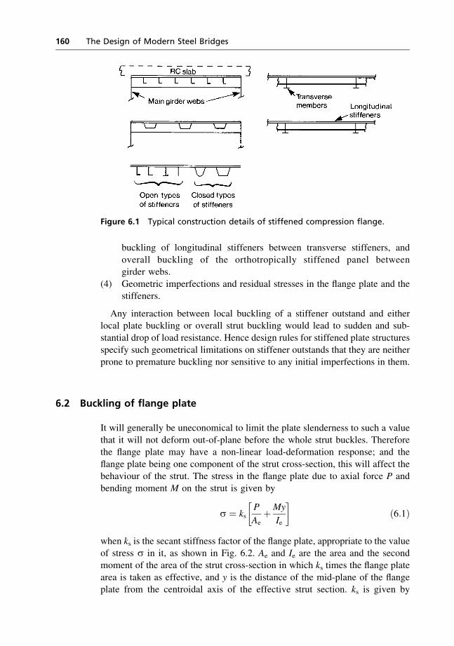
buckling of longitudinal stiffeners between transverse stiffeners, and

overall buckling of the orthotropically stiffened panel betweengirder webs.

(4) Geometric imperfections and residual stresses in the flange plate and thestiffeners.

Any interaction between local buckling of a stiffener outstand and eitherlocal plate buckling or overall strut buckling would lead to sudden and sub-

stantial drop of load resistance. Hence design rules for stiffened plate structuresspecify such geometrical limitations on stiffener outstands that they are neither

prone to premature buckling nor sensitive to any initial imperfections in them.

6.2 Buckling of flange plate

It will generally be uneconomical to limit the plate slenderness to such a valuethat it will not deform out-of-plane before the whole strut buckles. Thereforethe flange plate may have a non-linear load-deformation response; and the

flange plate being one component of the strut cross-section, this will affect thebehaviour of the strut. The stress in the flange plate due to axial force P and

bending moment M on the strut is given by

s ¼ ksP

AeþMy

Ie

� �ð6:1Þ

when ks is the secant stiffness factor of the flange plate, appropriate to the valueof stress s in it, as shown in Fig. 6.2. Ae and Ie are the area and the secondmoment of the area of the strut cross-section in which ks times the flange plate

area is taken as effective, and y is the distance of the mid-plane of the flangeplate from the centroidal axis of the effective strut section. ks is given by

Figure 6.1 Typical construction details of stiffened compression flange.


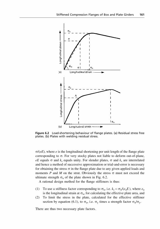
s/(eE), where e is the longitudinal shortening per unit length of the flange platecorresponding to s. For very stocky plates not liable to deform out-of-plane,

eE equals s and ks equals unity. For slender plates, s and ks are interrelatedand hence a method of successive approximation or trial-and-error is necessaryfor obtaining the stress s in the flange plate due to any given applied loads and

moments P and M on the strut. Obviously the stress s must not exceed theultimate strength su of the plate shown in Fig. 6.2.

A rational design method for the flange stiffeners is thus:

(1) To use a stiffness factor corresponding to su, i.e. ks¼su/(euE ), where euis the longitudinal strain at su, for calculating the effective plate area, and

(2) To limit the stress in the plate, calculated for the effective stiffener

section by equation (6.1), to su, i.e. sy times a strength factor su/sy.

There are thus two necessary plate factors.

Figure 6.2 Load-shortening behaviour of flange plates. (a) Residual stress freeplates. (b) Plates with welding residual stress.

Stiffened Compression Flanges of Box and Plate Girders 161

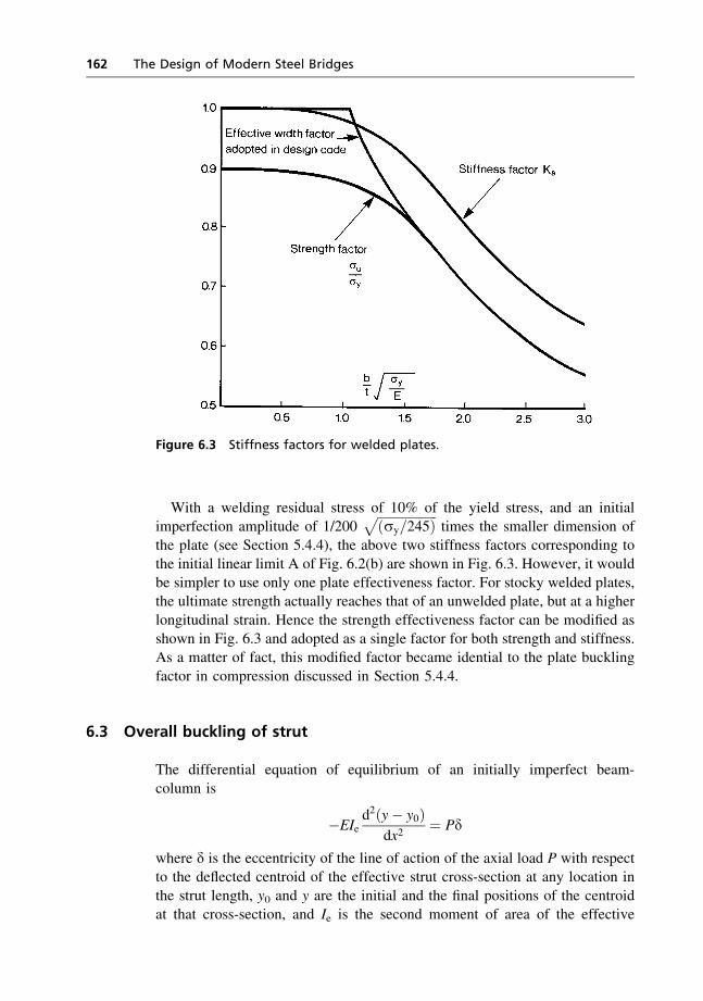
With a welding residual stress of 10% of the yield stress, and an initialimperfection amplitude of 1/200

ffiffiffiffiffiffiffiffiffiffiffiffiffiffiffiffiffiffiffiðsy=245Þp

times the smaller dimension of

the plate (see Section 5.4.4), the above two stiffness factors corresponding tothe initial linear limit A of Fig. 6.2(b) are shown in Fig. 6.3. However, it would

be simpler to use only one plate effectiveness factor. For stocky welded plates,the ultimate strength actually reaches that of an unwelded plate, but at a higher

longitudinal strain. Hence the strength effectiveness factor can be modified asshown in Fig. 6.3 and adopted as a single factor for both strength and stiffness.As a matter of fact, this modified factor became idential to the plate buckling

factor in compression discussed in Section 5.4.4.

6.3 Overall buckling of strut

The differential equation of equilibrium of an initially imperfect beam-

column is

�EIed2ðy� y0Þ

dx2¼ Pd

where d is the eccentricity of the line of action of the axial load P with respectto the deflected centroid of the effective strut cross-section at any location in

the strut length, y0 and y are the initial and the final positions of the centroidat that cross-section, and Ie is the second moment of area of the effective

Figure 6.3 Stiffness factors for welded plates.


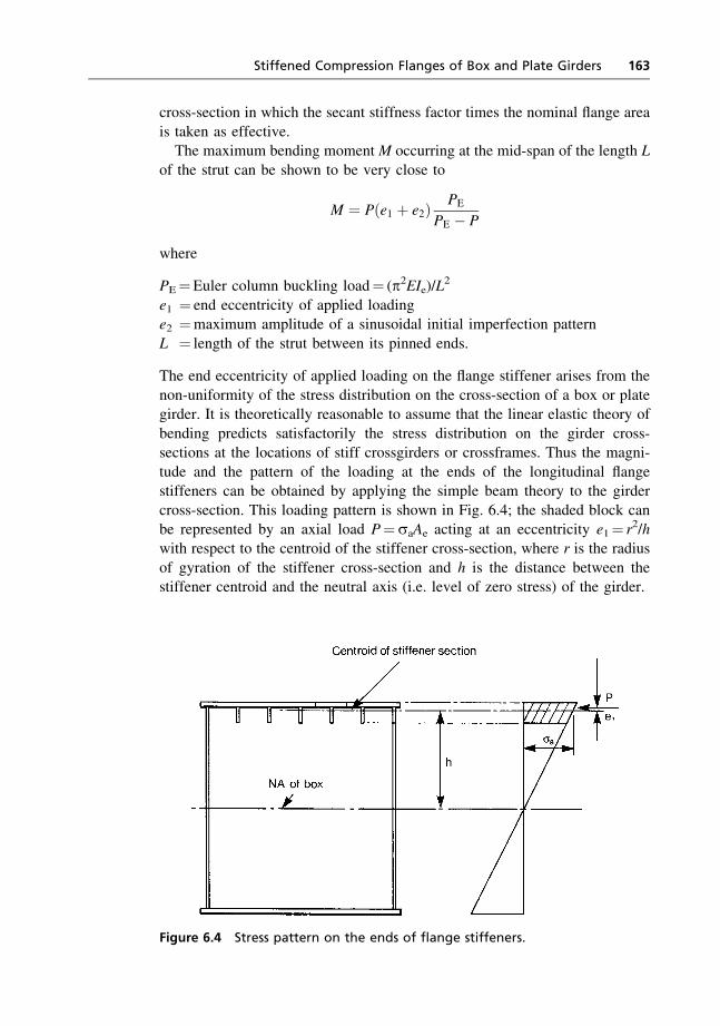
cross-section in which the secant stiffness factor times the nominal flange area

is taken as effective.The maximum bending moment M occurring at the mid-span of the length L

of the strut can be shown to be very close to

M ¼ Pðe1 þ e2Þ PE

PE � P

where

PE¼Euler column buckling load¼ (p2EIe)/L2

e1 ¼ end eccentricity of applied loadinge2 ¼maximum amplitude of a sinusoidal initial imperfection pattern

L ¼ length of the strut between its pinned ends.

The end eccentricity of applied loading on the flange stiffener arises from the

non-uniformity of the stress distribution on the cross-section of a box or plategirder. It is theoretically reasonable to assume that the linear elastic theory of

bending predicts satisfactorily the stress distribution on the girder cross-sections at the locations of stiff crossgirders or crossframes. Thus the magni-

tude and the pattern of the loading at the ends of the longitudinal flangestiffeners can be obtained by applying the simple beam theory to the girder

cross-section. This loading pattern is shown in Fig. 6.4; the shaded block canbe represented by an axial load P¼saAe acting at an eccentricity e1¼ r2/hwith respect to the centroid of the stiffener cross-section, where r is the radius

of gyration of the stiffener cross-section and h is the distance between thestiffener centroid and the neutral axis (i.e. level of zero stress) of the girder.

Figure 6.4 Stress pattern on the ends of flange stiffeners.


The well-known Perry strut equation can be used to obtain the limiting value

of the longitudinal stress that can be applied on the effective strut:

ssu

s0y

¼ 1

21þ ð1þ ZÞsE

s0y

( )�

ffiffiffiffiffiffiffiffiffiffiffiffiffiffiffiffiffiffiffiffiffiffiffiffiffiffiffiffiffiffiffiffiffiffiffiffiffiffiffiffiffiffiffiffiffiffiffiffiffiffiffiffi1þ ð1þ ZÞsE

s0y

( )2

� 4sE

s0y

vuut264

375 ð6:2Þ

where

ssu¼ limiting value of the applied longitudinal stress on the strut

sE ¼Euler buckling stress of the strutZ ¼�y/r2

� ¼maximum initial eccentricity and imperfection, i.e. (e1þ e2)

y ¼ distance of the extreme compressive fibre from the centroid of theeffective strut cross-section

r ¼ radius of gyration of the effective strut cross-sections0y ¼ available yield stress at the extreme compressive fibre (see Section 6.4).

Because of the asymmetry of the cross-section about the horizontal cen-

troidal axis, equation (6.2) must be applied to both the flange plate and the tipof the stiffening rib, with appropriate values for �, y and s0

y.

6.4 Allowance for shear and transverse stress in flange plate

According to Hencky–Mises’ criterion of yielding (see Chapter 2), the presenceof shear stress in the flange plate reduces its effective yield stress to

s0y ¼

ffiffiffiffiffiffiffiffiffiffiffiffiffiffiffiffiffiffis2y � 3t2

qð6:3Þ

The flange shear stress t is caused by (i) the vertical shear force on the cross-section of the main girder, and (ii) in the case of a box girder, by appliedtorsion on the girder. The stress due to (i) varies linearly from a maximum

value over the main girder web to zero mid-way between a pair of such webs,and hence only half the maximum value needs to be taken along with the full

value due to (ii) for t in equation (6.3) for the flange plate initiated failure. Forfailure initiated by the tip of the stiffeners, the full value of the material yield

stress of the tip is available in equation (6.2).In addition to the above influence on yield stress, shear stress due to torsion

on a box girder also causes a destabilising effect on the longitudinal flangestiffeners. An allowance for this may be made in the form of an additionalnotional axial load in the same way as derived for web stiffeners in Chapter 5.

Transverse stresses in the flange plate are caused by the flexure of thetransverse flange stiffeners, and crossframes and diaphragms in box girders. As

the centroid of the cross-section of a transverse stiffener is very near the flangeplate, the magnitude of the transverse stress is small. When this transverse

stress is compressive, it may in fact increase the effective yield stress in


longitudinal compression of the longitudinal stiffeners, as per Hencky–Mises’

yield criterion. Being localised, these transverse stresses are also not likely tocause any destabilising effects.

6.5 Orthotropic buckling of stiffened flange

Orthotropic buckling of the stiffened flange between the webs of the maingirders provides a restraining effect on the buckling of the longitudinal flange

stiffeners as individual parallel struts. This orthotropic behaviour produces twoseparate effects on the stress conditions of individual longitudinal stiffeners:

(1) Under the same magnitude of the applied longitudinal compressive loadacross the flange width, the magnification of the initial deflection of the

strut in an orthotropic panel is less than that of an isolated strut.(2) As the whole flange width between girder webs buckles, the applied longi-

tudinal compression varies across this width, with higher stresses along theedges (i.e. near the girder webs) and lower stresses along the central strips.

The word ‘orthotropic’ is an abbreviation of the feature ‘orthogonally aniso-

tropic’; in such a plate the lack of isotropy is due to different flexural rigiditiesin the orthogonal directions, even though the plate is of uniform thickness. Theelastic critical buckling stress of an orthotropic plate under longitudinal com-

pression, i.e. the value of the applied stress at which an ideally flat residual-stress-free orthotropic panel becomes unstable and suddenly deflects from its

initially flat plane, is given by

scro ¼ p2

tb2Dx

f2þ Dyf

2 þ 2H

� �ð6:4Þ

where

t ¼ thickness of the orthotropic plate

b ¼width of the orthotropic platea ¼ length of the orthotropic plate

Dx;Dy ¼ are the flexural rigidities in the x and y directions, respectivelyH ¼ torsional rigidity

f ¼ aspect ratio of the buckled panel, i.e. a/(mb)m ¼ number of half-waves in the longitudinal dimension a.

For a minimum value of scro, dscro/df¼ 0, i.e. f4¼Dx/Dy, leading to

scro ¼ 2p2

tb2ffiffiffiffiffiffiffiffiffiffiffiDxDy

p þ H � ð6:5Þ

and the half-wavelength of buckling l in the longitudinal direction is given by

l ¼ bDx

Dy

� �1=4


This buckling mode of the whole stiffened flange will involve interactive

buckling of both the longitudinal and the transverse stiffeners; this bucklingmode will not only be sensitive to the initial imperfections of the stiffeners, but

will be of a very ‘brittle’ nature, i.e. there will be a sudden and substantialshedding of the load at the onset of buckling. To avoid this catastrophic phe-

nomenon, the transverse stiffeners are normally designed to be sufficiently stiffnot to buckle when the longitudinal stiffeners do. Further reasons for making the

transverse stiffeners sufficiently stiff are that on the top flange they have tosupport without large deflection any locally applied axle loadings of vehicles,

and in box girders they form components of the internal crossframes or dia-phragms which are provided to prevent distortion of the box cross-section. Withsuch rigid transverse stiffeners the buckling of the stiffened flange will have one

half-wave in the longitudinal direction between adjacent transverse stiffeners.The rigidities Dx;Dy and H will thus not involve the geometric properties of the

transverse stiffener and will be given by

Dx ¼ EIxb 0 , Dy ¼ Et3

12ð1� v2Þ

H ¼ Gt3

6þ 1

2vyDx þ 1

2vxDy þ GJx

2b 0

9>>=>>; ð6:6Þ

where

Ix ¼ second moment of area of a longitudinal stiffenerb0 ¼ spacing of longitudinal stiffenerst ¼flange plate thickness

v ¼ Poisson’s ratio of the flange plateJx ¼ the torsional constant of the longitudinal stiffener

vx ¼ v½b0t=ðb0t þ AsxÞ�vy ¼ v

Asx ¼ cross-sectional area of one longitudinal stiffener.

For an ideal orthotropic plate, vyDx ¼ vxDy. In the case of a compression flangediscretely stiffened by longitudinal stiffeners between rigid transverse stif-

feners, this equality is not satisfied and the contribution of Dx towards thetorsional rigidity H is doubtful. Hence it is safe to take

H ¼ Gt3

6þ vxDy þ GJx

2b 0 ð6:7Þ

From equation (6.4), the total critical longitudinal compressive force in the

whole orthotropic panel will be

scrobt ¼ p2

b

Dx

f2þ Dyf

2 þ 2H

� �

The real orthotropic flange has discrete flange stiffeners, each of cross-sectional area Asx. If the width of the orthotropic flange panel between adjacent


webs of main girders is denoted by B, instead of b, the average critical stress on

the flange will be given by the above expression divided by Bt þ �Asx; i.e.

scro ¼ p2

B2 t þ �Asx

B

� Dx

f2þ Dyf

2 þ 2H

� �

The natural half-wavelength for the minimum value of scro should be

BðDx=DyÞ1=4; but for the orthotropic panel buckling between adjacent trans-verse stiffeners, Dx and Dy are given in equations (6.6) and ðDx=DyÞ will bevery large. Hence the actual half-wavelengths will be limited to the spacing Lbetween transverse stiffeners and f should be taken as L=B. This leads to

scro ¼ p2

t þ �Asx

B

� Dx

L2þ DyL

2

B4þ 2H

B2

� �ð6:8Þ

The minimum required stiffness Iy of transverse stiffeners, necessary to ensurethat overall buckling involving the transverse stiffeners is not more critical

than buckling between adjacent transverse stiffeners, may be obtained fromequations (6.5) and (6.8). For this purpose we may note that in applying (6.5)

we should take

Dy ¼ EIyL

, H ¼ Gt3

6þ GJx

2b0þ GJy

2L

and in applying (6.8) we should take

Dy ¼ Et3

12ð1� v2Þ , H ¼ Gt3

6þ vxDy þ GJx

2b0

For torsionally weak longitudinal and transverse stiffeners, i.e. open-type

stiffeners, H is negligible in applying (6.5), and both Dy and H are negligible inapplying (6.8). The minimum value of Iy of transverse stiffeners for suchstiffening, to ensure that overall buckling is less critical than buckling between

transverse stiffeners, is given by

2

B2

ffiffiffiffiffiffiffiffiffiffiffiDxDy

p>

Dx

L2

leading to

Iy >B4Ix4b0L3

ð6:9Þ

This is only true for elastic critical buckling of an ideally flat stiffened panel.

However, to prevent interactive buckling between local and overall modes,sudden drastic unloading and acute sensitivity to initial imperfections, Iyshould be several times the above value.For an isolated strut with a maximum initial out-of-straightness of e1 in a

sinusoidal mode, the magnification m of the out-of-straightness under an axial


load Pa is given by

m ¼ Pcr

Pcr � Pa

where Pcr is the Euler buckling load of the strut. The following cubic equation

gives the magnification m of the initial imperfection/eccentricity � of anorthotropically stiffened panel of length L between adjacent rigid transversestiffeners under the action of an applied compressive stress sa

sa ¼ scro � scro

mþ E�2

L2ðm2 � 1Þ ð6:10Þ

where scro is the elastic critical buckling compressive stress of the orthotropicpanel and � is the sum of the maximum initial out-of-straightness in length L

and any end eccentricity of the applied stress sa. The actual longitudinalstresses sc and se along the longitudinal centre line and edges, respectively, of

the orthotropic plate are given by

sc ¼ sa � 2E�2

L2ðm2 � 1Þ

se ¼ sa þ 2E�2

L2ðm2 � 1Þ

9>>=>>; ð6:11Þ

A longitudinal stiffener along or near the centre line is thus subject to:

(1) an axial force scAe, where Ae is the effective stiffener cross-section

(2) a maximum bending moment at its mid-span of

4pEIe�ðm� 1Þ=L2 ð6:12ÞA stiffener at or near the longitudinal edge is subject to:

(1) an axial force of seAe

(2) a bending moment of seAe�.

In an orthotropic stiffened panel, it is possible that all or most of thelongitudinal stiffeners in the cross-section may have high initial imperfections

e1 of similar magnitude; the end eccentricity e2 of the applied stress due tooverall bending of the whole box and plate girder is also the same for all

longitudinal stiffeners. The first Fourier series term for a constant value of(e1þ e2) across the whole width of the cross-section is 4/p (e1þ e2), andequations (6.10) to (6.12) take account of this increase in the effective value of

the imperfection.The effective cross-section of a central stiffener and also an edge stiffener

should be checked, with appropriate values and sign of �, so that the maxi-mum stress due to the above longitudinal axial loads and bending moments

does not exceed the effective yield stress of the flange plate given by equation(6.3) or the yield stress of the tip of the stiffener. The benefit of orthotropic


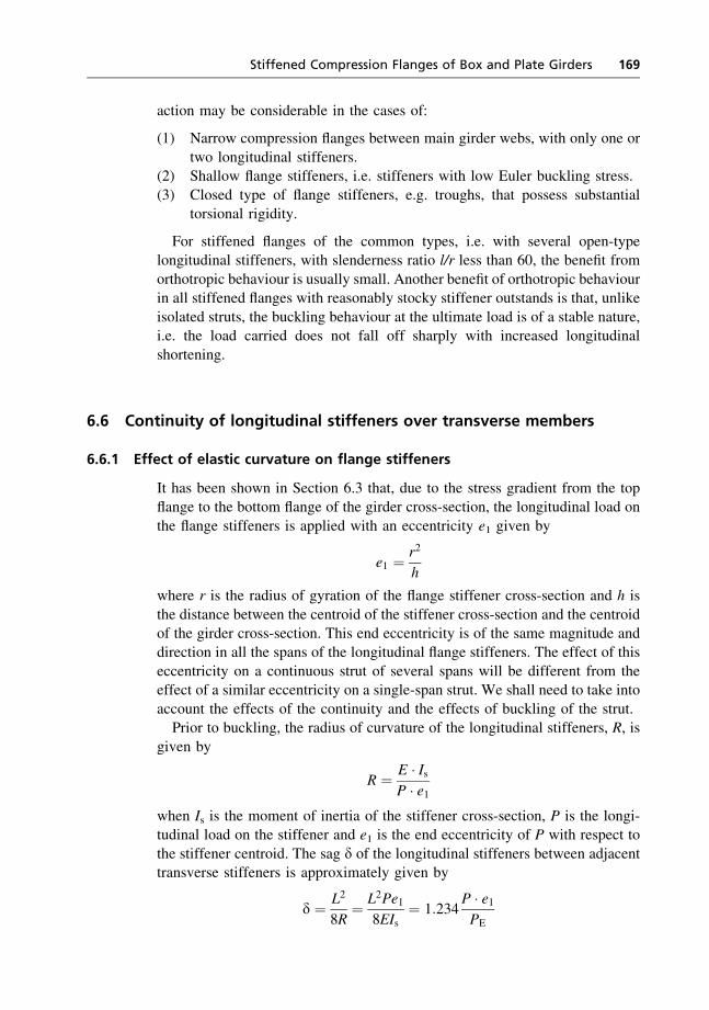
action may be considerable in the cases of:

(1) Narrow compression flanges between main girder webs, with only one or

two longitudinal stiffeners.(2) Shallow flange stiffeners, i.e. stiffeners with low Euler buckling stress.

(3) Closed type of flange stiffeners, e.g. troughs, that possess substantialtorsional rigidity.

For stiffened flanges of the common types, i.e. with several open-typelongitudinal stiffeners, with slenderness ratio l/r less than 60, the benefit from

orthotropic behaviour is usually small. Another benefit of orthotropic behaviourin all stiffened flanges with reasonably stocky stiffener outstands is that, unlike

isolated struts, the buckling behaviour at the ultimate load is of a stable nature,i.e. the load carried does not fall off sharply with increased longitudinal

shortening.

6.6 Continuity of longitudinal stiffeners over transverse members

6.6.1 Effect of elastic curvature on flange stiffeners

It has been shown in Section 6.3 that, due to the stress gradient from the topflange to the bottom flange of the girder cross-section, the longitudinal load on

the flange stiffeners is applied with an eccentricity e1 given by

e1 ¼ r2

h

where r is the radius of gyration of the flange stiffener cross-section and h is

the distance between the centroid of the stiffener cross-section and the centroidof the girder cross-section. This end eccentricity is of the same magnitude anddirection in all the spans of the longitudinal flange stiffeners. The effect of this

eccentricity on a continuous strut of several spans will be different from theeffect of a similar eccentricity on a single-span strut. We shall need to take into

account the effects of the continuity and the effects of buckling of the strut.Prior to buckling, the radius of curvature of the longitudinal stiffeners, R, is

given by

R ¼ E � IsP � e1

when Is is the moment of inertia of the stiffener cross-section, P is the longi-tudinal load on the stiffener and e1 is the end eccentricity of P with respect to

the stiffener centroid. The sag d of the longitudinal stiffeners between adjacenttransverse stiffeners is approximately given by

d ¼ L2

8R¼ L2Pe1

8EIs¼ 1:234

P � e1PE


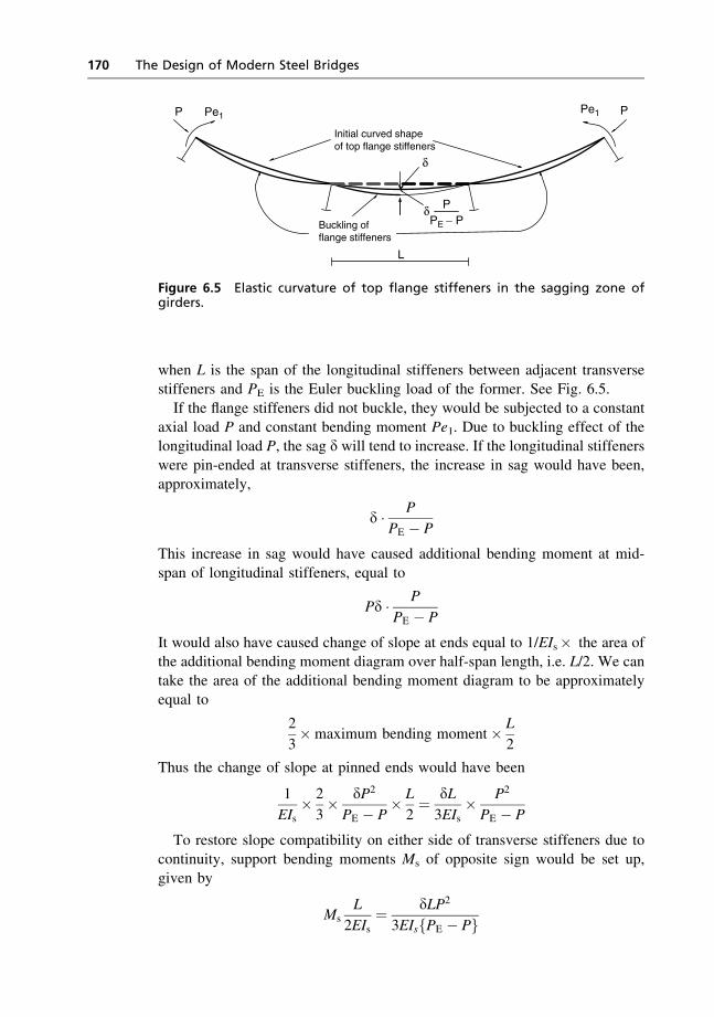
when L is the span of the longitudinal stiffeners between adjacent transversestiffeners and PE is the Euler buckling load of the former. See Fig. 6.5.

If the flange stiffeners did not buckle, they would be subjected to a constantaxial load P and constant bending moment Pe1. Due to buckling effect of thelongitudinal load P, the sag d will tend to increase. If the longitudinal stiffenerswere pin-ended at transverse stiffeners, the increase in sag would have been,approximately,

d � P

PE � P

This increase in sag would have caused additional bending moment at mid-

span of longitudinal stiffeners, equal to

Pd � P

PE � P

It would also have caused change of slope at ends equal to 1/EIs� the area ofthe additional bending moment diagram over half-span length, i.e. L/2. We can

take the area of the additional bending moment diagram to be approximatelyequal to

2

3�maximum bending moment� L

2

Thus the change of slope at pinned ends would have been

1

EIs� 2

3� dP2

PE � P� L

2¼ dL

3EIs� P2

PE � P

To restore slope compatibility on either side of transverse stiffeners due tocontinuity, support bending moments Ms of opposite sign would be set up,given by

MsL

2EIs¼ dLP2

3EIsfPE � Pg

Buckling offlange stiffeners

Initial curved shapeof top flange stiffeners

PE − P

δ

δ P

L

P Pe1 PPe1

Figure 6.5 Elastic curvature of top flange stiffeners in the sagging zone ofgirders.


wherefrom

Ms ¼ 2

3� dP2

PE � P

The net bending moment at mid-span of the longitudinal stiffeners is equal to

P � e1 þ d � P2

PE � P� 2

3� dP2

PE � P¼ P � e1 � 1þ 0:411

P2

PEfPE � Pg� �

since d¼ 1.234 ðPe1=PEÞ.If a pin-ended strut, with Euler buckling load PE and subjected to an axial

load P, had an initial imperfection eeff, then the maximum bending momentdue to buckling would be

P � eeff � PE

PE � P

Hence, for checking the mid-span section of the longitudinal stiffener as a

strut, we may assume the longitudinal stiffener to have an initial imperfectioneeff, given by

P � eeff � PE

PE � P¼ P � e1 1þ 0:411

P2

PEfPE � Pg� �

wherefrom

eeff ¼ k1e1, when k1 ¼ 1� P

PEþ 0:411

P

PE

� �2The direction of eeff is the same as the direction of e1, i.e. causing compressionon flange plate.The support section of the longitudinal stiffener needs to be checked to

ensure that yielding is not caused by the maximum fibre stress due to the axialload P and bending moment equal to

P � e1 �Ms

¼ P � e1 1� 0:823P2

PEfPE � Pg� �

¼ P � e1 � k2, when k2 ¼ 1� 0:823P2

PEfPE � PgFor various ratios of P/PE, the values of k1 and k2 are tabulated below:

P/PE k1 k2

0 1.0 1.00.2 0.816 0.959

0.4 0.666 0.7810.6 0.548 0.259

0.8 0.463 �1.634


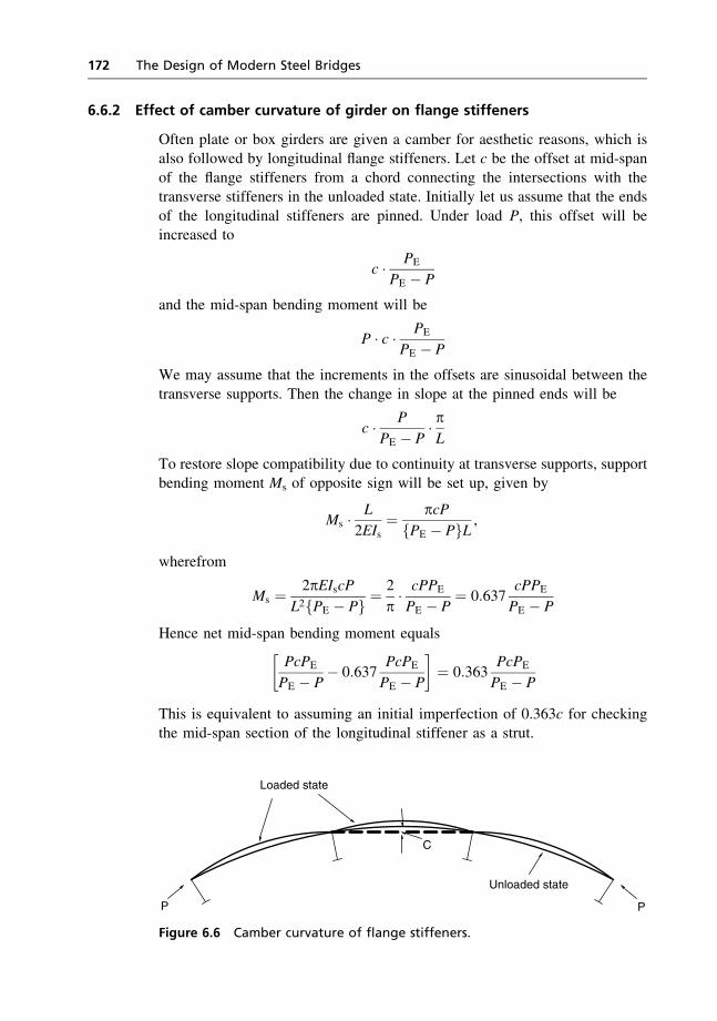
6.6.2 Effect of camber curvature of girder on flange stiffeners

Often plate or box girders are given a camber for aesthetic reasons, which isalso followed by longitudinal flange stiffeners. Let c be the offset at mid-span

of the flange stiffeners from a chord connecting the intersections with thetransverse stiffeners in the unloaded state. Initially let us assume that the ends

of the longitudinal stiffeners are pinned. Under load P, this offset will beincreased to

c � PE

PE � P

and the mid-span bending moment will be

P � c � PE

PE � P

We may assume that the increments in the offsets are sinusoidal between the

transverse supports. Then the change in slope at the pinned ends will be

c � P

PE � P� pL

To restore slope compatibility due to continuity at transverse supports, supportbending moment Ms of opposite sign will be set up, given by

Ms � L

2EIs¼ pcP

fPE � PgL ,

wherefrom

Ms ¼ 2pEIscPL2fPE � Pg ¼ 2

p� cPPE

PE � P¼ 0:637

cPPE

PE � P

Hence net mid-span bending moment equals

PcPE

PE � P� 0:637

PcPE

PE � P

� �¼ 0:363

PcPE

PE � P

This is equivalent to assuming an initial imperfection of 0.363c for checkingthe mid-span section of the longitudinal stiffener as a strut.

P

C

P

Loaded state

Unloaded state

Figure 6.6 Camber curvature of flange stiffeners.


The support section of the longitudinal stiffeners should be checked to

ensure that yielding is not caused by the maximum fibre stress due to axial loadP and bending moment equal to

0:637PcPE

PE � P

which is opposite in sign to the bending moment at mid-span caused by the

camber effect.

6.7 Local transverse loading on stiffened compression flange

The three-moment theorem for continuous beam columns[1] is suitable foranalysing a compression flange stiffener subjected to a local transverse loading

as well as the axial compression due to the overall bending moment on the boxor plate girder. In the case of an isolated simply supported column subjected to

a transverse load P as well, the deflected form and hence the bending momentsare found to be PE/(PE�P) times those values had there been no axial loading,

when PE is the Euler critical load of an isolated column. In the analysis ofa continuous beam column of several spans, the span moments are found to

increase by the above factor, but the support moments are found to hardlyincrease. Provided the axial loading is less than half the Euler buckling loadingof an isolated strut, the following method is appropriate for design:

(1) Calculate the bending moments due to local transverse loads on a

continuous beam, ignoring the axial load.(2) To obtain the design span moments, multiply the values obtained in (1)

by the factor PE/(PE�P).(3) For design support moments, take the values obtained in (1).

Assume sa to be the axial stress on the effective strut section due to the applied

axial load P, and sb to be the bending stress due to local transverse loadingcalculated without taking account of any axial loading. Then, with all the otherterms as defined in Section 6.3:

(1) For the mid-span region:

sa þ sa�y

r2þ sb

� �sE

sE � sa

� �>j s0

y

when s0y is the available yield stress at the extreme fibre (see Section 6.4).

It can be shown that the above criterion can also be approximately expressedby the following simpler equation:

sa

ssuþ sb

s0y

>j 1 ð6:13Þ

when ssu is the strength of a strut without any local transverse loading, for

which the effective material yield stress is s0y and as given by equation (6.2).


(2) For the support region:

sa þ sa�y

r2

� �sE

sE � sa

� �þ sb >j s0

y

or

sa þ sa�y

r2

� �sE

sE � sa

� �>j ðs0

y � sbÞ

or

sa >j Rs00y ð6:14aÞ

where Rs00y is the strut strength of a strut made of material yield stress s00

y,

and s00y ¼ s0

y � sb

and R is the ratio of the strut strength to material yield stress of a strut made ofmaterial yield stress s00

y .

Alternatively

sa

Rs0y

þ sb

s0y

>j 1 ð6:14bÞ

Comparing equation (6.13) with this equation, it should be noted that ssu isless than Rs0

y, as R is calculated for a strut of a lower effective material yield

stress s00y; this reflects the benefit of the applied bending moment not being

magnified by the axial load over the support section.

6.8 Effect of variation in the bending moment of a girder

The applied axial stress in a longitudinal stiffener in a stiffened flange varies

according to the shape of the bending moment diagram on the box or plategirder. Such a stiffener may be checked as a uniformly compressed strut with

an equivalent applied axial load equal to that occurring at a distance 0.4L fromthe heavily stressed end. However, for a relatively slender strut, i.e. one with

high ‘l/r’ ratio, subjected to a substantial variation in the axial loading at itstwo ends, such an approximate method may be too conservative. A more accur-

ate method, in which the magnitude and location of the maximum bendingmoment is calculated for such a strut with initial out-of-straightness imper-fection, is given in Reference [2].

6.9 Transverse stiffeners in stiffened compression flanges

In the design of longitudinal stiffeners, it has been assumed that the transversestiffeners shall provide adequate support to the longitudinal stiffeners, so that


the effective buckling length of the latter does not exceed their span between

the former, i.e. the transverse stiffeners form non-deflecting nodal lines in thebuckling mode of the whole stiffened flange. Comparing the elastic critical

buckling stresses for the buckling mode between adjacent transverse stiffenersand that involving their deflection, the minimum flexural rigidity of the trans-

verse stiffener has been derived in equation (6.9) for a stiffened panel of ‘open’type, i.e. torsionally weak stiffeners. This approach may be: (i) too conser-

vative in some cases, as the flexural stiffness of the longitudinal stiffeners maybe unnecessarily larger than that required for the longitudinal loading they

carry; and (ii) too optimistic in other cases, as interactive buckling between thelocal mode (i.e. between transverse stiffeners) and the overall mode (i.e.involving deflection of transverse stiffeners) may produce a brittle type of

failure with sudden and substantial fall-off in the applied loading. A morerational approach is to provide sufficient flexural rigidity of the transverse stif-

feners so that there is a substantial safety factor over the magnitude of theapplied loading against overall elastic critical buckling involving the deflection

of transverse stiffeners.The elastic critical buckling stress given by equation (6.4) has been derived

for one isolated orthotropically stiffened panel, with the longitudinal edgessimply supported. The overall elastic critical buckling stress of the entire widthof a stiffened compression flange supported by several main girder webs and

thus comprising several internal panels and one or two cantilever panels, iscomplex. There will be some interaction between adjacent panels if they are of

different widths, through some rotational restraint at the common edge, but themagnitude of such interaction at the ultimate limit state is uncertain. For those

reasons it is advisable to divide the whole width of the stiffened flange intoa number of independent longitudinal panels and to calculate the critical

buckling stress separately for each panel, i.e. assuming no interaction betweenadjacent panels. A cantilever panel on its own, i.e. without any rotational

restraint at the supported longitudinal edge, tends to buckle in a mode whichremains virtually straight in the transverse direction at all transverse sectionsand with very long half-wavelengths in the longitudinal direction; as a conse-

quence the elastic critical buckling load is found to be almost entirely con-tributed by the torsional rigidity of the longitudinal stiffeners. For a stiffened

flange with torsionally weak, i.e. ‘open’, type longitudinal stiffeners, the canti-lever panels are virtually unstable unless they are combined with the adjacent

panel or panels with both longitudinal edges simply supported. There are thusthree types of deck panels to be considered, namely a deck panel without any

cantilevers, a deck panel with one cantilever, and a deck panel with two canti-levers. For a stiffened flange with torsionally weak longitudinal stiffeners, theelastic critical buckling load per unit width of the stiffened flange is given by

pcr ¼ 4

B2

EcIcEfIfY

L

� �1=2ð6:15Þ


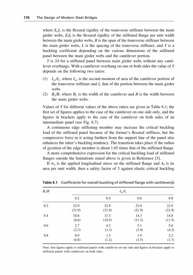
where EcIc is the flexural rigidity of the transverse stiffener between the main

girder webs, EfIf is the flexural rigidity of the stiffened flange per unit widthbetween the main girder webs, B is the span of the transverse stiffener between

the main girder webs, L is the spacing of the transverse stiffener, and Y is abuckling coefficient depending on the various dimensions of the stiffened

panel between the main girder webs and the cantilever portion.Y is 24 for a stiffened panel between main girder webs without any canti-

lever overhangs. With a cantilever overhang on one or both sides the value of Ydepends on the following two ratios:

(1) Icc/Ic, where Icc is the second moment of area of the cantilever portion ofthe transverse stiffener and Ic that of the portion between the main girder

webs(2) Bc/B, where Bc is the width of the cantilever and B is the width between

the main girder webs.

Values of Y for different values of the above ratios are given in Table 6.1; thefirst set of figures applies to the case of the cantilever on one side only, and the

figures in brackets apply to the case of the cantilever on both sides of anintermediate panel (see Fig. 6.7).A continuous edge stiffening member may increase the critical buckling

load of the stiffened panel because of the former’s flexural stiffness, but thecompressive force in it acting furthest from the support line of the panel also

enhances the latter’s buckling tendency. The transition takes place if the radiusof gyration of the edge member is about 1.65 times that of the stiffened flange.

A more comprehensive expression for the critical buckling load of stiffenedflanges outside the limitations stated above is given in Reference [3].

If sa is the applied longitudinal stress on the stiffened flange and Af is itsarea per unit width, then a safety factor of 3 against elastic critical buckling

Table 6.1 Coefficients for overall buckling of stiffened flange with cantilever(s)

Bc/B Icc/Ic

0.2 0.4 0.6 0.8

0.2 22.9 22.9 22.9 22.9(21.9) (21.9) (21.9) (21.9)

0.4 10.8 13.3 14.3 14.8(8.6) (10.5) (11.2) (11.5)

0.6 2.7 4.2 5.1 5.6(2.3) (3.3) (3.9) (4.2)

0.8 0.9 1.5 1.9 2.2(0.8) (1.2) (1.5) (1.7)

Note: first figures apply to stiffened panels with cantilever on one side and figures in brackets apply to

stiffened panels with cantilevers on both sides.


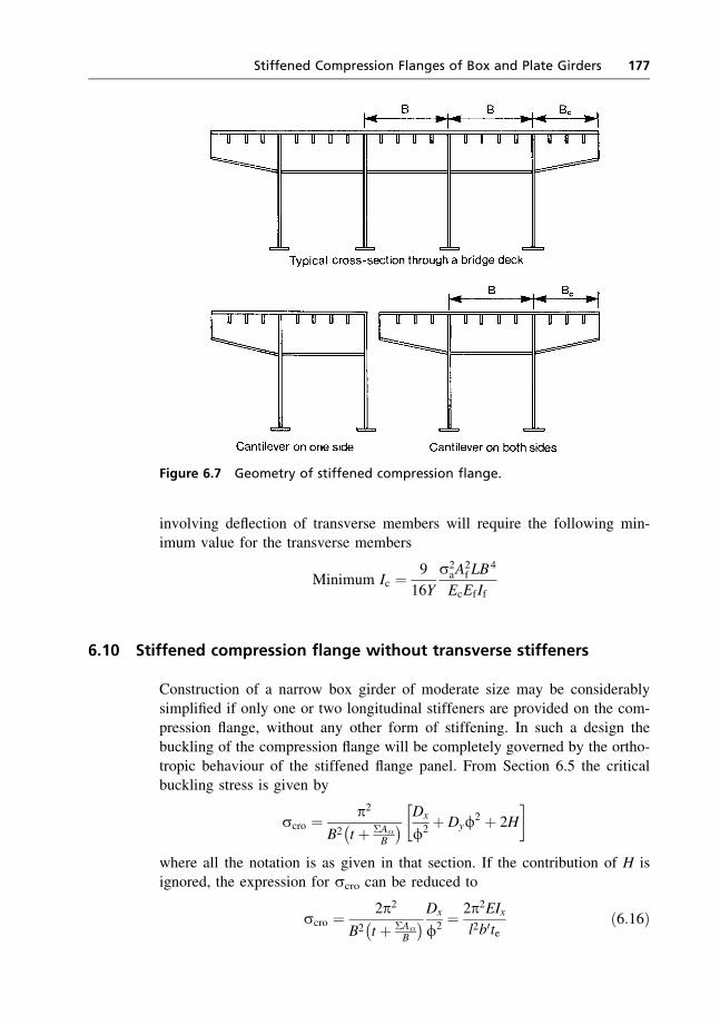
involving deflection of transverse members will require the following min-imum value for the transverse members

Minimum Ic ¼ 9

16Y

s2aA

2f LB

4

EcEfIf

6.10 Stiffened compression flange without transverse stiffeners

Construction of a narrow box girder of moderate size may be considerablysimplified if only one or two longitudinal stiffeners are provided on the com-

pression flange, without any other form of stiffening. In such a design thebuckling of the compression flange will be completely governed by the ortho-

tropic behaviour of the stiffened flange panel. From Section 6.5 the criticalbuckling stress is given by

scro ¼ p2

B2 t þ �Asx

B

� Dx

f2þ Dyf

2 þ 2H

� �

where all the notation is as given in that section. If the contribution of H isignored, the expression for scro can be reduced to

scro ¼ 2p2

B2 t þ �Asx

B

� Dx

f2¼ 2p2EIx

l2b0teð6:16Þ

Figure 6.7 Geometry of stiffened compression flange.


where

l ¼ buckling half-wavelength¼BðDx=DyÞ0:25f ¼ l/Bte ¼ effective thickness¼ tþð�AsxÞ=BB ¼width of flange between websIx ¼moment of inertia of one flange stiffener

b0 ¼ spacing between stiffeners.

The above expression shows that an individual flange stiffener can be deemed

to be an isolated Euler strut with an effective length Le given by

Le ¼ lffiffiffi2

p ¼ Bffiffiffi2

p Dx

Dy

� �0:25

We know that

Dx ¼ EIxb0

¼ EIxðN þ 1ÞB

and

Dy ¼ Et3

12ð1� v2Þwhere

N¼ number of flange stiffeners in flange width Bv¼ Poission’s ratio¼ 0.3.

Hence

Le ¼ Bffiffiffi2

p 12IxðN þ 1Þð1� v2ÞBt3

� �0:25

¼ 1:285B

t

� �0:75

IxðN þ 1Þ½ �0:25

To be on the conservative side, it is advisable to take

L ¼ 1:5B

t

� �0:25

IxðN þ 1Þ½ �0:25 ð6:17Þ

6.11 A design example of stiffened compression flange

Applied longitudinal stresses due to factored loads are shown below; furtherpartial safety factors of gf3¼ 1.1 and gm¼ 1.20 are to be allowed for.A flange stiffener can be taken as a strut composed of a flange plate 375� 25

and an angle 200� 100� 12 (Fig. 6.8).


The geometrical properties of this strut are:

Centroidal moment of inertia, Ix ¼ 64 840 298mm4

Area of cross-section¼ 12 831mm2

Radius of gyration, r¼ 71.09mmMaximum fibre distance to the top¼ 50.54mm

Maximum fibre distance to the bottom ¼ 174.46mm.

Distance between stiffener centroid and girder neutral axis, h¼ 897�50.54¼ 846.46mm; e1¼ eccentricity of applied loading¼ r2=h¼ 5.97mm.

(a) Effective eccentricity for checking mid-span section of flange stiffener

¼ k1e1; when k1 ¼ 1� sa

sEþ 0:411

sa

sE

� �2sa ¼ applied axial stress ¼ 145:6N=mm2

sE ¼ Euler stress ¼ p2Eð71:09Þ2ð3000Þ2 ¼ 1136N=mm2

k1 ¼ 0:8786

Effective eccentricity of applied loading¼ 5.25mm; e2¼ amplitude ofinitial imperfection¼ 3000/625¼ 4.80mm; �1¼ k1e1þ e2¼ 10.05 mm.

(i) For checking failure due to compression in flange plate

Z ¼ 10:05� 50:54

ð71:09Þ2 ¼ 0:1005

The ultimate stress ssu is given by

Figure 6.8 Details of a design example of a stiffened compression flange.


ssu

355¼ 1

21þ 1:1005

1136

355

� ��

ffiffiffiffiffiffiffiffiffiffiffiffiffiffiffiffiffiffiffiffiffiffiffiffiffiffiffiffiffiffiffiffiffiffiffiffiffiffiffiffiffiffiffiffiffiffiffiffiffiffiffiffiffiffiffiffiffiffiffiffiffiffiffiffi1þ 1:1005

1136

355

� �2

� 4� 1136

355

s24

35

¼ 1

2½4:5216� 2:7649�

¼ 0:8783

ssu ¼ 311:8N=mm2

ssu

gmgf3¼ 311:8

1:20� 1:1¼ 236:2N=mm2 > 145:6N=mm2

(ii) The outstand tip should be checked for possible failure due to either

compressive or tensile stress. For maximum compression, �¼ 4.80�5.25¼�0.45mm. Hence flexure will cause tensile stress at outstand tip,

and total stress will be compressive and less than 145.6N/mm2. Formaximum tension at outstand tip, �¼ 10.05mm. Maximum tensilestress

¼ �145:6þ 145:6� 12 831� 10:05

64:84� 106� 174:46� 1136

ð1136� 145:6Þ¼ �145:6þ 57:92N=mm2

i.e. no tensile stress.

(b) The support section of the longitudinal flange stiffener should be checkedfor maximum stress at flange plate and at outstand tip. Effectiveeccentricity¼ k2� 5.97mm, when

k2 ¼ 1� 0:823s2a

sEðsE � saÞ¼ 0:9845

Compressive stress on flange plate

¼ 145:6þ 145:6� 12 831� 5:97� 0:9845� 50:54

64:84� 106

¼ 145:6þ 8:56 ¼ 154:16N=mm2

Compressive stress at outstand tip

¼ 145:6� 145:6� 12 831� 5:97� 0:9845� 174:46

64:84� 106

¼ 145:6� 29:54 ¼ 116:06N=mm2

These stresses are not critical. Hence the flange stiffener is satisfactory.


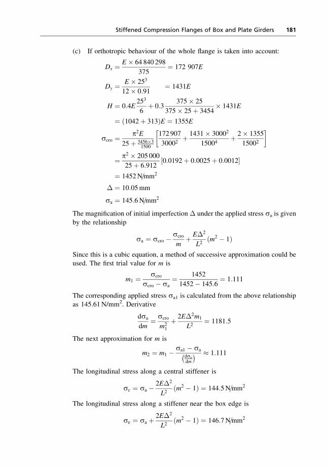
(c) If orthotropic behaviour of the whole flange is taken into account:

Dx ¼ E � 64 840 298

375¼ 172 907E

Dy ¼ E � 253

12� 0:91¼ 1431E

H ¼ 0:4E253

6þ 0:3

375� 25

375� 25þ 3454� 1431E

¼ ð1042þ 313ÞE ¼ 1355E

scro ¼ p2E25þ 3456�3

1500

172 907

30002þ 1431� 30002

15004þ 2� 1355

15002

� �

¼ p2 � 205 000

25þ 6:9120:0192þ 0:0025þ 0:0012½ �

¼ 1452N=mm2

� ¼ 10:05mm

sa ¼ 145:6N=mm2

The magnification of initial imperfection� under the applied stress sa is given

by the relationship

sa ¼ scro � scro

mþ E�2

L2ðm2 � 1Þ

Since this is a cubic equation, a method of successive approximation could beused. The first trial value for m is

m1 ¼ scro

scro � sa¼ 1452

1452� 145:6¼ 1:111

The corresponding applied stress sa1 is calculated from the above relationship

as 145.61N/mm2. Derivative

dsa

dm¼ scro

m21

þ 2E�2m1

L2¼ 1181:5

The next approximation for m is

m2 ¼ m1 � sa1 � sa

dso

dm

� � 1:111

The longitudinal stress along a central stiffener is

sc ¼ sa � 2E�2

L2ðm2 � 1Þ ¼ 144:5N=mm2

The longitudinal stress along a stiffener near the box edge is

se ¼ sa þ 2E�2

L2ðm2 � 1Þ ¼ 146:7N=mm2


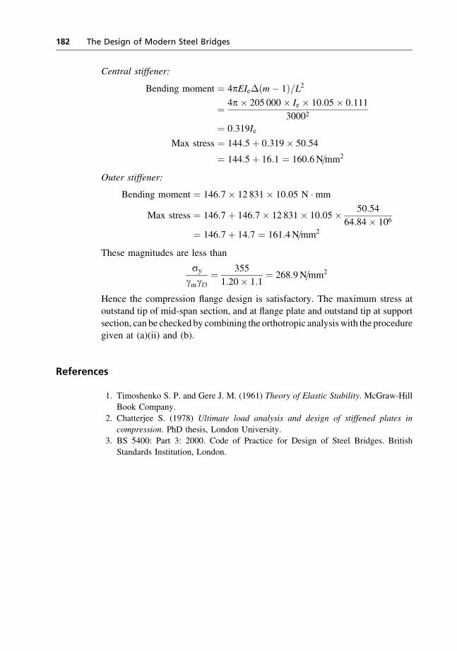
Central stiffener:

Bending moment ¼ 4pEIe�ðm� 1Þ=L2

¼ 4p� 205 000� Ie � 10:05� 0:111

30002

¼ 0:319Ie

Max stress ¼ 144:5þ 0:319� 50:54

¼ 144:5þ 16:1 ¼ 160:6N=mm2

Outer stiffener:

Bending moment ¼ 146:7� 12 831� 10:05 N �mm

Max stress ¼ 146:7þ 146:7� 12 831� 10:05� 50:54

64:84� 106

¼ 146:7þ 14:7 ¼ 161:4N=mm2

These magnitudes are less than

sy

gmgf3¼ 355

1:20� 1:1¼ 268:9N=mm2

Hence the compression flange design is satisfactory. The maximum stress atoutstand tip of mid-span section, and at flange plate and outstand tip at support

section, can be checked by combining the orthotropic analysiswith the proceduregiven at (a)(ii) and (b).

References

1. Timoshenko S. P. and Gere J. M. (1961) Theory of Elastic Stability. McGraw-Hill

Book Company.

2. Chatterjee S. (1978) Ultimate load analysis and design of stiffened plates in

compression. PhD thesis, London University.

3. BS 5400: Part 3: 2000. Code of Practice for Design of Steel Bridges. British



Chapter 7

Cable-stayed Bridges

7.1 History

A brief history of cable-stayed type of bridge construction is included in

Chapter 1. This section provides a more detailed account of the gradual techno-logical developments leading up to the present state-of-the-art of this type of

bridges.The concept of providing intermediate support to a beam by inclined ties

hanging from a tower or mast dated back to ancient times. The Egyptians builtsailing ships by applying this idea. In the Far East, rivers were spanned by

bamboo bridges supported by vines attached to trees on the banks. In 1617Faustus Verantius of Venice designed a timber deck bridge supported byseveral inclined eye-bars attached to masonry towers, and in 1784 a German

carpenter Immanuel Loscher built in Freibourg a 32m span timber bridgesupported by timber stays attached to a timber tower[1]. In 1817 British

engineers Redpath and Brown built the 33.6m span King’s Meadowsfootbridge using inclined wire cables to support lattice longitudinal girders

in the outer thirds of their spans from the tops of two cast-iron towers. Quite afew bridges were subsequently built in various parts of Europe, with wrought

iron bars, chains, wires or even timber stays supporting metal or timber decksfrom towers; but many of them collapsed in strong wind. These stays could not

be tightened during erection and hence they were only effective after a sub-stantial deflection of the deck. Cable stays were successfully adopted by JohnRoebling in America to provide crucially needed extra stiffness and aero-

dynamic stability to his great suspension bridges, the first being the GrandTrunk Bridge across the Niagara opened in 1885, then the bridge over the Ohio

in Cincinnati opened in 1867, and the most striking being the Brooklyn Bridgein New York (Figure 1.9) opened in 1883. The Franz Joseph Bridge in Prague

and the Albert Bridge in London (Figure 1.8) designed by Ordish and openedin 1868 and 1873, respectively, had a combination of suspension and stay rods,

but the cable formed by the suspension rods was used only to hold the diagonalstay rods. In the second half of the nineteenth century in France Arnodin builtseveral bridges of span up to 163m with the central portion of the span

supported by hangers from two suspension cables and stay cables radiatingfrom the tower tops supporting the outer portions of the span. This system

183

reduced the deflection of the bridge, and as the stay cables did not go as far as

the mid-span region, the height of the towers was also reduced. The first success-ful bridge supported only by cable stays were by Giscard in France at the turn of

the century, who developed a system of triangulation with stays in a fanarrangement radiating from tower tops intersecting with near-horizontal cables

stretched between the towers that took up the horizontal component of thetension in the stay cables. With this system the need for substantial anchorage

structure was eliminated. An example of this system was the Cassagne Bridgewith a central span of 156m built in 1907. Le Cocq modified Giscard’s system

by transferring the horizontal components of the stay cable forces to the stiffeninggirder and built in 1925 the Lezardrieux Bridge over the Trieux river in 1925.The first modern cable-stayed bridge was the Stromsund bridge in Sweden

designed by Dischinger and built by Demag Company of Germany in 1956,with a main span of 183m and two-side spans of 75m. Two planes of cable

stays had two pairs of cables radiating in a fan shape from the tops of portal-frame towers. Two fabricated steel plate girders were used as stiffening girders

just outside the two cable planes. Assuming static distribution of deck loadingbetween the stiffening girders, the structural system in each cable plane had 10

redundancies, viz. eight cable tensions and two vertical reactions; but makinguse of symmetry/antisymmetry about the transverse axis of the bridge reducedthe redundancy to four, which was just within the capability of manual

numerical calculation. Thus all cable tensions and stiffening girder deflectionswere accurately calculated at all stages of construction.

Bridging the navigable river Rhine demanded clear spans over 250m. Theconfidence with the cable-stayed type of bridges, and a parallel development of

the orthotropic steel deck system, which substantially reduced the weight ofthe deck, led to the building of a remarkable series of visually exciting and

economical bridges in Germany after the Second World War. The TheodorHeuss Bridge across the Rhine at Dusseldorf, opened in 1957, had spans of

108–260–108m and had three sets of parallel cables from each tower in eachdirection in two cable planes, fixed at three points in the tower height in what isnow called a ‘harp’ configuration. The stiffening system consisted of two box

girders along the cable planes; their torsional rigidity affected the transversedistribution of deck loading between the cable planes, thus doubling the

structural redundancies. An accurate analysis of this system was far beyond thecapacity of the manual/slide rule facilities of those days, hence approximations

had to be made. The harp arrangement of cables was theoretically less efficientthan the fan arrangement, as the cable inclinations were less steep. An

orthotropic welded steel deck spanned between the longitudinal box girders tocarry traffic, but also contributed to resist the longitudinal compression arisingfrom the cable tensions.

The next cable-stayed bridge, the Severins across the Rhine at Koln, wasopened in 1960 and became famous for its single A-shaped tower on one bank

through which two unequal spans of 302 and 151m ‘floated’. Three pairs of


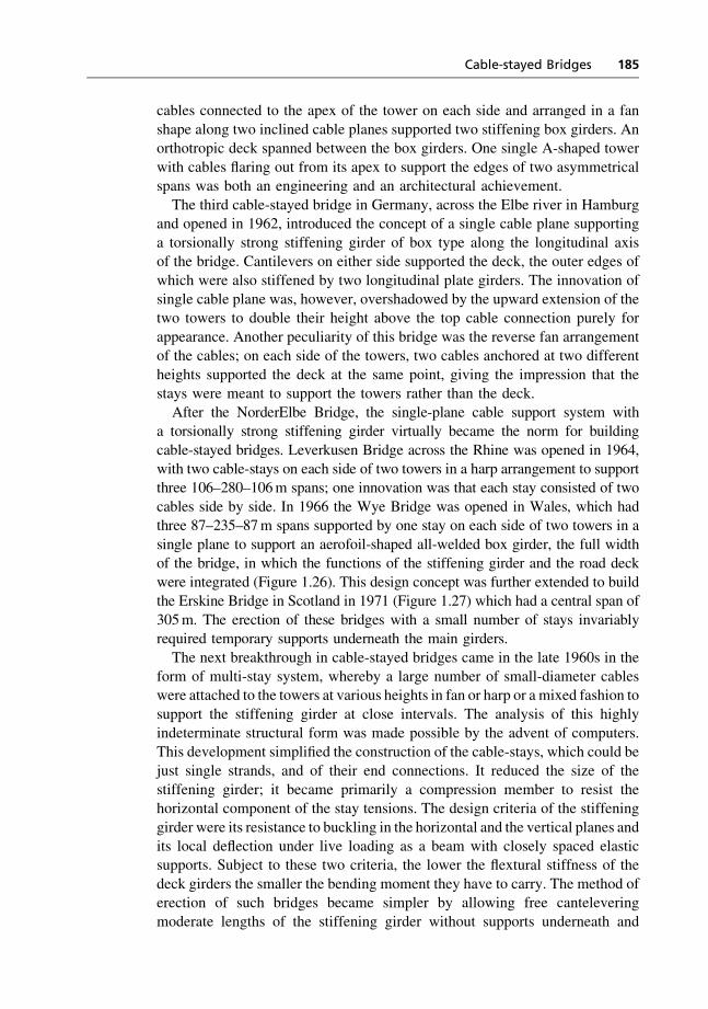
cables connected to the apex of the tower on each side and arranged in a fan

shape along two inclined cable planes supported two stiffening box girders. Anorthotropic deck spanned between the box girders. One single A-shaped tower

with cables flaring out from its apex to support the edges of two asymmetricalspans was both an engineering and an architectural achievement.

The third cable-stayed bridge in Germany, across the Elbe river in Hamburgand opened in 1962, introduced the concept of a single cable plane supporting

a torsionally strong stiffening girder of box type along the longitudinal axisof the bridge. Cantilevers on either side supported the deck, the outer edges of

which were also stiffened by two longitudinal plate girders. The innovation ofsingle cable plane was, however, overshadowed by the upward extension of thetwo towers to double their height above the top cable connection purely for

appearance. Another peculiarity of this bridge was the reverse fan arrangementof the cables; on each side of the towers, two cables anchored at two different

heights supported the deck at the same point, giving the impression that thestays were meant to support the towers rather than the deck.

After the NorderElbe Bridge, the single-plane cable support system witha torsionally strong stiffening girder virtually became the norm for building

cable-stayed bridges. Leverkusen Bridge across the Rhine was opened in 1964,with two cable-stays on each side of two towers in a harp arrangement to supportthree 106–280–106m spans; one innovation was that each stay consisted of two

cables side by side. In 1966 the Wye Bridge was opened in Wales, which hadthree 87–235–87m spans supported by one stay on each side of two towers in a

single plane to support an aerofoil-shaped all-welded box girder, the full widthof the bridge, in which the functions of the stiffening girder and the road deck

were integrated (Figure 1.26). This design concept was further extended to buildthe Erskine Bridge in Scotland in 1971 (Figure 1.27) which had a central span of

305m. The erection of these bridges with a small number of stays invariablyrequired temporary supports underneath the main girders.

The next breakthrough in cable-stayed bridges came in the late 1960s in theform of multi-stay system, whereby a large number of small-diameter cableswere attached to the towers at various heights in fan or harp or a mixed fashion to

support the stiffening girder at close intervals. The analysis of this highlyindeterminate structural form was made possible by the advent of computers.

This development simplified the construction of the cable-stays, which could bejust single strands, and of their end connections. It reduced the size of the

stiffening girder; it became primarily a compression member to resist thehorizontal component of the stay tensions. The design criteria of the stiffening

girder were its resistance to buckling in the horizontal and the vertical planes andits local deflection under live loading as a beam with closely spaced elasticsupports. Subject to these two criteria, the lower the flextural stiffness of the

deck girders the smaller the bending moment they have to carry. The method oferection of such bridges became simpler by allowing free cantelevering

moderate lengths of the stiffening girder without supports underneath and

Cable-stayed Bridges 185

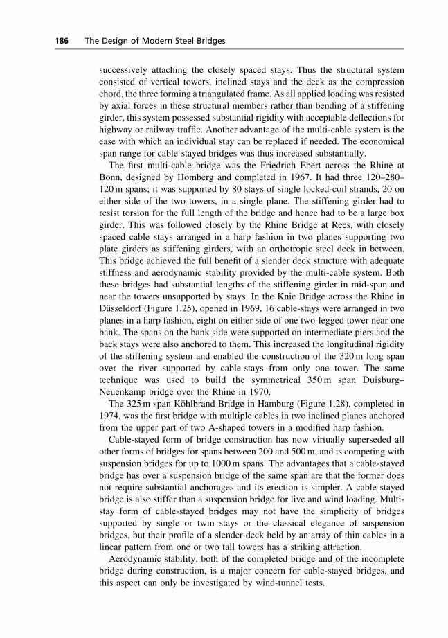
successively attaching the closely spaced stays. Thus the structural system

consisted of vertical towers, inclined stays and the deck as the compressionchord, the three forming a triangulated frame. As all applied loading was resisted

by axial forces in these structural members rather than bending of a stiffeninggirder, this system possessed substantial rigidity with acceptable deflections for

highway or railway traffic. Another advantage of the multi-cable system is theease with which an individual stay can be replaced if needed. The economical

span range for cable-stayed bridges was thus increased substantially.The first multi-cable bridge was the Friedrich Ebert across the Rhine at

Bonn, designed by Homberg and completed in 1967. It had three 120–280–120m spans; it was supported by 80 stays of single locked-coil strands, 20 oneither side of the two towers, in a single plane. The stiffening girder had to

resist torsion for the full length of the bridge and hence had to be a large boxgirder. This was followed closely by the Rhine Bridge at Rees, with closely

spaced cable stays arranged in a harp fashion in two planes supporting twoplate girders as stiffening girders, with an orthotropic steel deck in between.

This bridge achieved the full benefit of a slender deck structure with adequatestiffness and aerodynamic stability provided by the multi-cable system. Both

these bridges had substantial lengths of the stiffening girder in mid-span andnear the towers unsupported by stays. In the Knie Bridge across the Rhine inDusseldorf (Figure 1.25), opened in 1969, 16 cable-stays were arranged in two

planes in a harp fashion, eight on either side of one two-legged tower near onebank. The spans on the bank side were supported on intermediate piers and the

back stays were also anchored to them. This increased the longitudinal rigidityof the stiffening system and enabled the construction of the 320m long span

over the river supported by cable-stays from only one tower. The sametechnique was used to build the symmetrical 350m span Duisburg–

Neuenkamp bridge over the Rhine in 1970.The 325m span Kohlbrand Bridge in Hamburg (Figure 1.28), completed in

1974, was the first bridge with multiple cables in two inclined planes anchoredfrom the upper part of two A-shaped towers in a modified harp fashion.Cable-stayed form of bridge construction has now virtually superseded all

other forms of bridges for spans between 200 and 500m, and is competing withsuspension bridges for up to 1000m spans. The advantages that a cable-stayed

bridge has over a suspension bridge of the same span are that the former doesnot require substantial anchorages and its erection is simpler. A cable-stayed

bridge is also stiffer than a suspension bridge for live and wind loading. Multi-stay form of cable-stayed bridges may not have the simplicity of bridges

supported by single or twin stays or the classical elegance of suspensionbridges, but their profile of a slender deck held by an array of thin cables in alinear pattern from one or two tall towers has a striking attraction.

Aerodynamic stability, both of the completed bridge and of the incompletebridge during construction, is a major concern for cable-stayed bridges, and

this aspect can only be investigated by wind-tunnel tests.


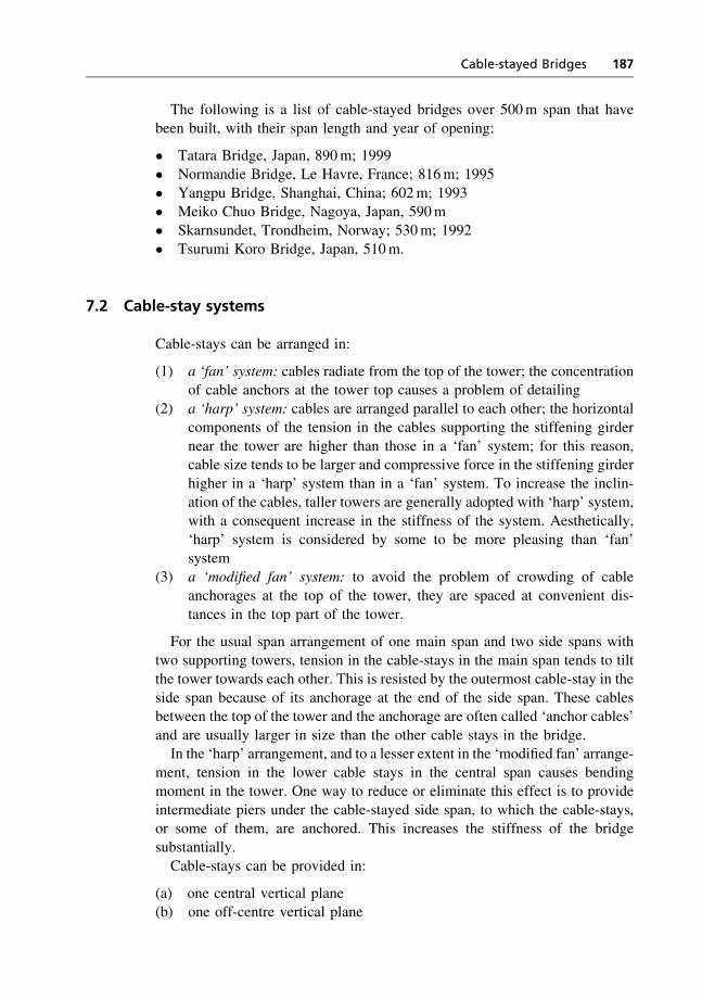
The following is a list of cable-stayed bridges over 500m span that have

been built, with their span length and year of opening:

� Tatara Bridge, Japan, 890m; 1999� Normandie Bridge, Le Havre, France; 816m; 1995

� Yangpu Bridge, Shanghai, China; 602m; 1993� Meiko Chuo Bridge, Nagoya, Japan, 590m

� Skarnsundet, Trondheim, Norway; 530m; 1992� Tsurumi Koro Bridge, Japan, 510m.

7.2 Cable-stay systems

Cable-stays can be arranged in:

(1) a ‘fan’ system: cables radiate from the top of the tower; the concentrationof cable anchors at the tower top causes a problem of detailing

(2) a ‘harp’ system: cables are arranged parallel to each other; the horizontalcomponents of the tension in the cables supporting the stiffening girder

near the tower are higher than those in a ‘fan’ system; for this reason,cable size tends to be larger and compressive force in the stiffening girderhigher in a ‘harp’ system than in a ‘fan’ system. To increase the inclin-

ation of the cables, taller towers are generally adopted with ‘harp’ system,with a consequent increase in the stiffness of the system. Aesthetically,

‘harp’ system is considered by some to be more pleasing than ‘fan’system

(3) a ‘modified fan’ system: to avoid the problem of crowding of cableanchorages at the top of the tower, they are spaced at convenient dis-

tances in the top part of the tower.

For the usual span arrangement of one main span and two side spans with

two supporting towers, tension in the cable-stays in the main span tends to tiltthe tower towards each other. This is resisted by the outermost cable-stay in the

side span because of its anchorage at the end of the side span. These cablesbetween the top of the tower and the anchorage are often called ‘anchor cables’

and are usually larger in size than the other cable stays in the bridge.In the ‘harp’ arrangement, and to a lesser extent in the ‘modified fan’ arrange-

ment, tension in the lower cable stays in the central span causes bendingmoment in the tower. One way to reduce or eliminate this effect is to provide

intermediate piers under the cable-stayed side span, to which the cable-stays,or some of them, are anchored. This increases the stiffness of the bridgesubstantially.

Cable-stays can be provided in:

(a) one central vertical plane(b) one off-centre vertical plane


(c) two vertical planes, with twin-leg tower

(d) two inclined planes, with A-shaped tower.

With (a) or (b), the stiffening girder must be torsionally strong and must besupported at the tower on bearings to resist torsion. With (c) or (d), the cables

can be attached to the deck either at its edges or within its width; in the lattercase the configuration/clearance of the traffic paths will have to be safe-

guarded. The width of the tower foundation normal to the bridge directioncould be shorter with (a) or (b) than with (c) or (d). It is not essential to supportthe stiffening girder at the tower on bearings if cable supports are provided all

along its length and in two planes; that way a hard point on the stiffening girderwith high hogging bending moment is avoided. However, if the stiffening

girder is supported on bearings at the tower and by multiple cable-stays ineither a single or twin planes, stays can be omitted for some distance either side

of the tower. That solution creates a window in the cable net either side of thetower, which is often admired as an attractive architectural feature.

The tower need not be vertical; it can be tilted towards the side span, withboth architectural and structural advantages; but the tower will have to be

supported by temporary stays in the bridge direction during construction. Therecould also be different stay arrangements in the central and side spans; forexample, stays in a single central vertical plane in the central span and in two

inclined planes in the side spans meeting at the tower was adopted for the Ebrobridge in Spain.

All the possible arrangements for stay cables described above for three-spancable-stayed bridges with two towers are also possible for two-span bridges

with one tower on one bank of a river.As outlined in Section 7.1, the earlier cable-stayed bridges had only a few

cable-stays but modern bridges tend to have a large number of small diametercable-stays. Figures 7.1 and 7.2 show, in conceptual forms, various arrange-ments of stays in cable-stayed bridges.

7.3 Cable types

The basic element of the cable-stays is the steel wire 5 to 7mm diameter with

proof (or yield) and ultimate strengths of the order of 1200 and 1600N/mm2,respectively, as against 450 and 600N/mm2 for high-tensile structural steel.

These steel wires are cold-drawn from high-carbon pearlitic rolled rods. Thetensile strength of such wires has improved from about 1000N/mm2 in the1880s, when Brooklyn Bridge was built, to about 1300N/mm2 in the 1900s,

and then to around 1500N/mm2 in the 1930s. No great advance has beenachieved since then. Wires with tensile strength of 1600N/mm2 are now avail-

able. In Japan attempts are being made to produce wires of 1900N/mm2 tensilestrength. Such high strengths are obtained by a high percentage of carbon in


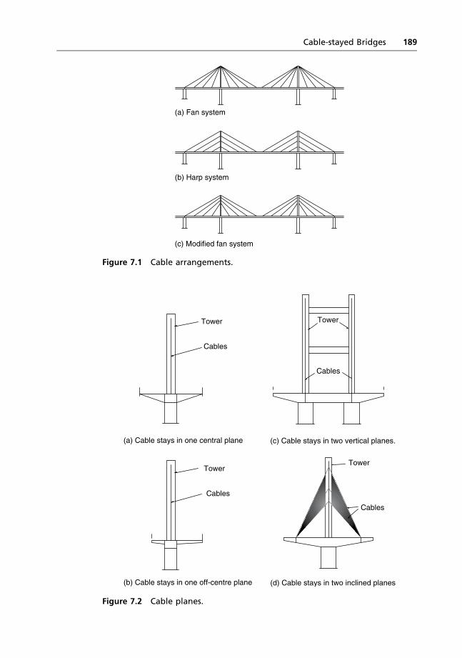
(a) Fan system

(b) Harp system

(c) Modified fan system

Figure 7.1 Cable arrangements.

Tower

Cables

Cables

TowerTower

Cables

Cables

Tower

(a) Cable stays in one central plane

(b) Cable stays in one off-centre plane (d) Cable stays in two inclined planes

(c) Cable stays in two vertical planes.

Figure 7.2 Cable planes.


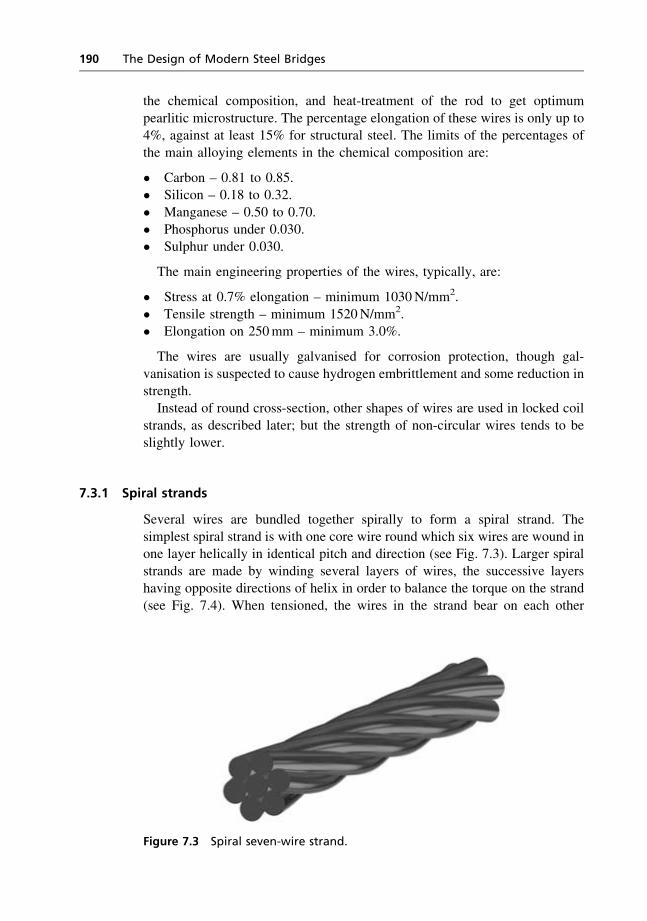
the chemical composition, and heat-treatment of the rod to get optimum

pearlitic microstructure. The percentage elongation of these wires is only up to4%, against at least 15% for structural steel. The limits of the percentages of

the main alloying elements in the chemical composition are:

� Carbon – 0.81 to 0.85.� Silicon – 0.18 to 0.32.

� Manganese – 0.50 to 0.70.� Phosphorus under 0.030.� Sulphur under 0.030.

The main engineering properties of the wires, typically, are:

� Stress at 0.7% elongation – minimum 1030N/mm2.

� Tensile strength – minimum 1520N/mm2.� Elongation on 250mm – minimum 3.0%.

The wires are usually galvanised for corrosion protection, though gal-

vanisation is suspected to cause hydrogen embrittlement and some reduction instrength.Instead of round cross-section, other shapes of wires are used in locked coil

strands, as described later; but the strength of non-circular wires tends to beslightly lower.

7.3.1 Spiral strands

Several wires are bundled together spirally to form a spiral strand. Thesimplest spiral strand is with one core wire round which six wires are wound inone layer helically in identical pitch and direction (see Fig. 7.3). Larger spiral

strands are made by winding several layers of wires, the successive layershaving opposite directions of helix in order to balance the torque on the strand

(see Fig. 7.4). When tensioned, the wires in the strand bear on each other

Figure 7.3 Spiral seven-wire strand.


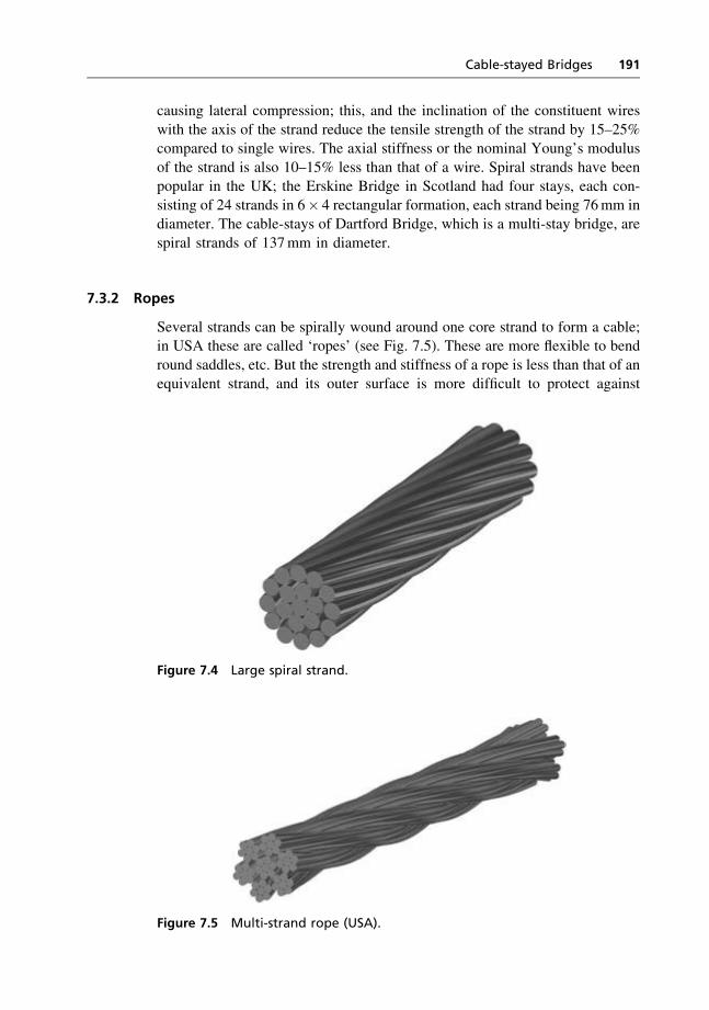
causing lateral compression; this, and the inclination of the constituent wires

with the axis of the strand reduce the tensile strength of the strand by 15–25%compared to single wires. The axial stiffness or the nominal Young’s modulus

of the strand is also 10–15% less than that of a wire. Spiral strands have beenpopular in the UK; the Erskine Bridge in Scotland had four stays, each con-

sisting of 24 strands in 6� 4 rectangular formation, each strand being 76mm indiameter. The cable-stays of Dartford Bridge, which is a multi-stay bridge, are

spiral strands of 137mm in diameter.

7.3.2 Ropes

Several strands can be spirally wound around one core strand to form a cable;in USA these are called ‘ropes’ (see Fig. 7.5). These are more flexible to bend

round saddles, etc. But the strength and stiffness of a rope is less than that of anequivalent strand, and its outer surface is more difficult to protect against

Figure 7.4 Large spiral strand.

Figure 7.5 Multi-strand rope (USA).


corrosion. In Britain the term rope usually means a strand with only one layer

of wires wound helically around a core wire.The first tensioning of a helical strand causes an irreversible elongation due

to radial compaction of the constituent layers. To avoid this non-elastic elonga-tion in first service loading, the strand is prestretched with a tension 10–20%

above the maximum tension that the strand will be subjected to during service.

7.3.3 Locked-coil strands

In Germany ‘locked-coil spiral strands’ have been developed to produce morecompact cables with a smoother outer surface for more effective corrosion

protection. The longitudinal stiffness of locked-coil spiral strands are aboutmid-way between those of straight wires and ordinary spiral strands. Locked-

coil strands experience less lateral pressure at saddles, sockets and anchorages.Wires of different cross-sectional shapes are used in different layers to achieve

surface, rather than point, contact between wires. For example, a normal strandwith round wires is wound with one or more layers of wedge-shaped wires,

with the outermost one or two layers made up of wires of S-shaped cross-section (see Fig 7.6). These specially shaped wires fit tightly together to form acompact cable with about 90% material density, as against about 70% in spiral

strands with round wires. The tensile strength of shaped wires is slightly lessthan that of round wires. In Germany the wires of locked coil strands were

usually not galvanised, in order to avoid possible hydrogen embrittlement. Thefirst modern cable-stayed bridge, the Stromsund in Sweden, had 16 stays each

made up of four locked-coil strands of 66 or 88mm in diameter. Each staycable of the multi-stay Chao Paya Bridge in Bangkok is 167mm diameter

locked-coil strand.

Figure 7.6 Locked-coil spiral strand.


The spiral winding of wires around a centroidal axis enable the strands to be

coiled or reeled for transport and handling. For the same reason they can beeasily bent or draped over saddles, etc. Because spiral strands are self-

compacting when under even a small tension, they need not be held by cir-cumferential bands to keep the wires together.

7.3.4 Parallel-wire strands

The reduction of strength and axial stiffness caused by twisting of wires in

spiral strands led to the development of parallel-wire strands, notably in Japan.Cables of parallel-wire strands are prefabricated with all wires straight from

end to end. But the difficulties of transportation and handling of long lengthsof cables inspired investigations into the feasibility of their reeling. It was

discovered in the USA that such cables could be reeled in drums of appropriatesize without unacceptable permanent deformation, as some local twisting of

the cable and slight opening out of some of the wires between clamping bandstook place. Upon unreeling the strands were found to recover their original

shape and compactness and strength tests indicated no fall. Parallel-wire strandsare usually fabricated to pure or near hexagonal shapes. A large parallel-wirestrand can be used as one cable-stay; in Parana Bridges in Argentina parallel-

wire strand stays consisted of 337 number 7mm wires assembled in a near-round form. A multiple number of parallel-wire strands are sometimes bundled

to form one large cable; the Yamatogawa Bridge in Japan has 16 cable-stayseach of which is made up of 19 parallel-wire strands, each strand containing

217 galvanised wires of 5mm diameter.In cable-stayed bridges each cable-stay can consist of a single spiral or

parallel-wire strand or a rope, as usually the case in bridges with multiple cable-stays, or a group of strands when the cable size is large, e.g. in a long spansupported by only a few large cables. The strands in the group may be held

closely together, or kept separate but in particular formation. When a largenumber of spiral strands are held together, usually inside a tube, the cable is

sometimes called ‘parallel-strand cable’. Freyssinet, Dywidag and VSL com-panies offer proprietory strand systems of this kind, often using seven-wire

strands.

7.3.5 Long-lay cables

The concept of long-lay spiral cable has the aim of achieving reeling withouta reduction in strength or axial stiffness that is associated with spiral laying.

A lay angle of upto 4 degrees has been found to achieve these aims. The firstmajor use of such cables was in the Annacis Bridge in Vancouver, Canada,

where cables of up to 130mm diameter were made up with galvanised bridgestrands. The Yokohama Bay Bridge in Japan also used such cables.


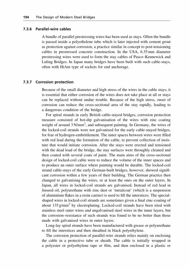
7.3.6 Parallel-wire cables

A bundle of parallel prestressing wires has been used as stays. Often the bundleis passed inside a polyethelene tube which is later injected with cement grout

as protection against corrosion, a practice similar in concept to post-tensioningcables in prestressed concrete construction. In the USA, 6.35mm diameter

prestressing wires were used to form the stay cables of Pasco–Kennewick andLuling Bridges. In Japan many bridges have been built with such cable-stays,

often with HiAm type of sockets for end anchorage.

7.3.7 Corrosion protection

Because of the small diameter and high stress of the wires in the cable stays, it

is essential that either corrosion of the wires does not take place at all or stayscan be replaced without undue trouble. Because of the high stress, onset of

corrosion can reduce the cross-sectional area of the stay rapidly, leading toa dangerous condition of the bridge.

For spiral strands in early British cable-stayed bridges, corrosion protectionmeasure consisted of hot-dip galvanisation of the wires with zinc coating

weight of around 3N/mm2, and subsequent painting. In Germany, the wires ofthe locked-coil strands were not galvanised for the early cable-stayed bridges,

for fear of hydrogen-embrittlement. The inner spaces between wires were filledwith red lead during the formation of the cable, to prevent collection of mois-ture that would initiate corrosion. After the stays were erected and tensioned

with the dead load of the bridge, the stay surfaces were throughly cleaned andthen coated with several coats of paint. The main aims of the cross-sectional

design of locked-coil cable were to reduce the volume of the inner spaces andto produce an outer surface where painting would be durable. The locked-coil

strand cable-stays of the early German-built bridges, however, showed signifi-cant corrosion within a few years of their building. The German practice then

changed to galvanising the wires, or at least the ones on the outer layers. InJapan, all wires in locked-coil strands are galvanised. Instead of red lead inlinseed oil, polyurethane with zinc dust or ‘metalcoat’ (which is a suspension

of aluminium flakes in a resin carrier) is used to fill the interstices. The special-shaped wires in locked-coil strands are sometimes given a final zinc-coating of

about 135 g/mm2 by electroplating. Locked-coil strands have been tried withstainless steel outer wires and ungalvanised steel wires in the inner layers, but

the corrosion–resistance of such strands was found to be no better than thosemade with galvanised wires in outer layers.

Long-lay spiral strands have been manufactured with grease or polyurethaneto fill the interstices and then sheathed in black polyethylene.

The corrosion protection of parallel-wire strands relies mainly on enclosingthe cable in a protective tube or sheath. The cable is initially wrapped ina polyester or polyethylene tape or film, and then enclosed in a plastic or


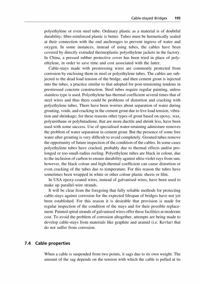
polyethylene or even steel tube. Ordinary plastic as a material is of doubtful

durability; fibre-reinforced plastic is better. Tubes must be hermetically sealedat their connection with the end anchorages to prevent ingress of water and

oxygen. In some instances, instead of using tubes, the cables have beencovered by directly extruded thermoplastic polyethylene jackets in the factory.

In China, a pressed rubber protective cover has been tried in place of poly-ethylene, in order to save time and cost associated with the latter.

Cable-stays made with prestressing wires are commonly protected fromcorrosion by enclosing them in steel or polyethylene tubes. The cables are sub-

jected to the dead load tension of the bridge, and then cement grout is injectedinto the tubes, a practice similar to that adopted for post-tensioning tendons inprestressed concrete construction. Steel tubes require regular painting, unless

stainless type is used. Polyethylene has thermal coefficient several times that ofsteel wires and thus there could be problems of distortion and cracking with

polyethylene tubes. There have been worries about separation of water duringgrouting, voids, and cracking in the cement grout due to live load tension, vibra-

tion and shrinkage; for these reasons other types of grout based on epoxy, wax,polyurethane or polybutadiene, that are more ductile and shrink less, have been

used with some success. Use of specialised water-retaining admixture removesthe problem of water separation in cement grout. But the presence of some freewater after grouting is very difficult to avoid completely. Grouted tubes remove

the opportunity of future inspection of the condition of the cables. In some casespolyethylene tubes have cracked, probably due to thermal effects and/or pro-

longed or too-small-radius reeling. Polyethylene tubes are black in colour, dueto the inclusion of carbon to ensure durability against ultra-violet rays from sun;

however, the black colour and high-thermal coefficient can cause distortion oreven cracking of the tubes due to temperature. For this reason the tubes have

sometimes been wrapped in white or other colour plastic sheets or film.In USA epoxy-coated wires, instead of galvanised wires, have been used to

make up parallel-wire strands.It will be clear from the foregoing that fully reliable methods for protecting

cable-stays against corrosion for the expected lifespan of bridges have not yet

been established. For this reason it is desirable that provision is made forregular inspection of the condition of the stays and for their possible replace-

ment. Painted spiral strands of galvanised wires offer these facilities at moderatecost. To avoid the problem of corrosion altogether, attempts are being made to

develop cable-stays from materials like graphite and aramid (i.e. Kevlar) thatdo not suffer from corrosion.

7.4 Cable properties

When a cable is suspended from two points, it sags due to its own weight. The

amount of the sag depends on the tension with which the cable is pulled at its


ends. If the weight of the cable is uniform along its length, the deflected shape

of the cable will be a catenary. The analysis of the catenary shape is muchmore complicated than that of a parabola, which would have been the deflected

shape of the cable if its weight were uniformly distributed on the horizontalprojected length of the cable. The error caused by this approximation on the

length, sag or tension of the cable is found to be insignificant for practicalimplications in even the extreme real-life cases. The relationship between the

sag and the tension in the cable can be obtained by equating the bendingmoment at mid-length of the cable to zero and is given by

f ¼ wL2

8H¼ gC2

8sð7:1Þ

where

f ¼ vertical sag

w¼weight of cable per unit horizontal lengthL ¼ horizontal span between cable anchorages

H¼ horizontal component of the cable tensiong ¼weight per unit volume of the cable materialC¼ inclined distance between cable anchorages

s¼ tensile stress in the cable.

It may be noted that the vertical sag of the cable is inversely proportional tothe tension in it.

Due to the sag the curved length of the cable is larger than the chord length by

8f 2

3L sec3 y

where y is the angle of the cable with the horizontal.Due to the tension s the cable will have stretched elastically by an amount

Cs/E; hence the length of the unstressed cable (i.e. lying on the ground)should be

C þ 8f 2

3C sec2 y� Cs

Eð7:2Þ

The self-weight of the cable reduces the cable tension in the bottom half ofthe cable and increases the cable tension in the top half; the tension in the cable

will be maximum at its top end and minimum at the bottom; the maximumtension is given by

H 1þ h

Lþ 4f

L

� �2( )1=2

where

H¼ horizontal component of the cable tension at the ends andh ¼ vertical distance between the cable anchorages.


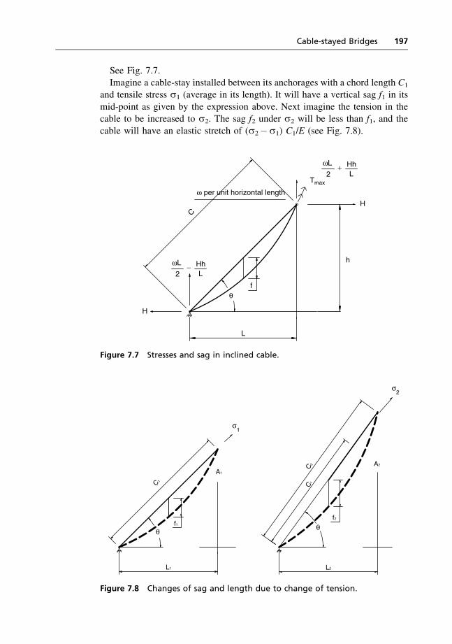
See Fig. 7.7.

Imagine a cable-stay installed between its anchorages with a chord length C1

and tensile stress s1 (average in its length). It will have a vertical sag f1 in its

mid-point as given by the expression above. Next imagine the tension in thecable to be increased to s2. The sag f2 under s2 will be less than f1, and the

cable will have an elastic stretch of (s2�s1) C1/E (see Fig. 7.8).

L

f

h

H

2Hh

ω per unit horizontal length

Tmax

ωL

L+

C

2HhωL

L−

H

θ

Figure 7.7 Stresses and sag in inclined cable.

C1

f1

A1

L2L1

f2

A2C2

σ2

θ θ

σ1

C1

Figure 7.8 Changes of sag and length due to change of tension.


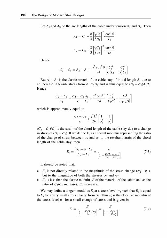
Let A1 and A2 be the arc lengths of the cable under tension s1 and s2. Then

A1 ¼ C1 þ 8

3

gC 21

8s1

� �2� cos

3 yL1

A2 ¼ C2 þ 8

3

gC 22

8s2

� �2� cos

3 yL2

Hence

C2 � C1 ¼ A2 � A1 þ g2 cos3 y24

C 41

s21L1

� C 42

s22L 2

� �

But A2�A1 is the elastic stretch of the cable-stay of initial length A1 due toan increase in tensile stress from s1 to s2 and is thus equal to (s2�s1)A1/E.

Hence

C2 � C1

C1¼ s2 � s1

E

A1

C1þ g2 cos3 y

24

C31

L1s21

� C 42

C1L2s22

� �

which is approximately equal to

s2 � s1

Eþ g2L2

24

1

s21

� 1

s22

� �

(C2�C1)/C1 is the strain of the chord length of the cable stay due to a change

in stress of (s2�s1). If we define Es as a secant modulus representing the ratioof the change of stress between s1 and s2 to the resultant strain of the chordlength of the cable-stay, then

Es ¼ ½s2 � s1�C1

C2 � C1¼ E

1þ Eg2L224

s1þs2

s21s22

h i ð7:3Þ

It should be noted that:

� Es is not directly related to the magnitude of the stress change (s2�s1),but to the magnitude of both the stresses s1 and s2

� Es is less than the elastic modulus E of the material of the cable; and as theratio of s2/s1 increases, Es increases.

We may define a tangent modulus Et at a stress level s1 such that Et is equal

to Es for a very small stress change from s1. Thus Et is the effective modulus atthe stress level s1 for a small change of stress and is given by

Et ¼ E

1þ Eg2L224

2s1

s41

h i ¼ E

1þ Eg2L2

12s31

h i ð7:4Þ


It may be noted that:

� Et is higher with larger values of s1 and approaches the value of the materialelastic modulus E with very high value of s1.

7.5 Design and construction of a cable-stayed bridge

The erection of the deck structure commences by erecting a deck segment onthe pier support and on a temporary support at the far end of the segment. The

first cable-stay is then attached between the tower and the far end of the decksegment, and is tensioned to the right pre-calculated value, at the same timelifting the far end of the segment to the right pre-calculated level. The next

deck segment is then attached to and cantilevered out of the far end of theprevious segment. The next cable stay is then attached between the tower and

the far end of the cantilevered deck segment and is tensioned to the right pre-calculated value, lifting the far end to the right pre-calculated level. Erection of

deck segments continues on both sides of the tower, i.e. on both main and sidespans, keeping a balance between the bending moments on the two sides of the

tower. Erection also proceeds from the other tower in the same way, until allthe deck segments are erected, except for a small length in the centre of themain span. In the final step, after having checked and adjusted the profile levels

and the cable-stay tensions, the closing piece is inserted between andconnected to the two cantilevered edges of the main span deck segments.

It is essential to obtain the correct cable tensions and correct levels of thedeck profile at all stages of the erection sequence, in order to achieve the

correct profile of the completed bridge. The evaluation of the correct cabletensions and the correct profile of bridge at various stages of erection can be

done by a reverse process of the erection sequence, as described below:

(a) The starting point of this procedure is the final required profile of the

whole length of the completed bridge. The tensions in all the stay-cables can bechosen freely by trial and error so that, under the dead weight of the bridge and

the action of the cable tensions, including the buckling effect of the compres-sive forces on the stiffening girder, i.e. horizontal components of the cable

forces, the flexural deflections of the stiffening girder conform to the specifiedprofile of the bridge. The cable tensions may be the same for all the cables, or

proportional to their sizes; alternatively, their vertical components may be thesame. The total of the vertical components of cable forces will need to be slightly

greater than the total dead load of the deck, in order to achieve a hogging orarch profile of the bridge.

(b) In the next step, imagine removing the superimposed dead load, i.e. all

non-structural carriageway fittings like barriers, handrails, wearing courses,etc. From the structural model of the bridge that includes the stiffening girders,

the cable-stays and the towers, obtain the changes in the bending moments of


the stiffening girders, the changes in the cable tensions and the changes in the

bridge profile due to the removal of the superimposed dead loads. For thisexercise, the cable stiffnesses should be based on their tangent modulus given

by equation (7.4), corresponding to the assumed tension in the cables for thecompleted bridge. After obtaining the reduction in the cable tensions, the process

should be reiterated with the cable stiffness based on their secant modulusgiven by equation (7.3), appropriate to their initial tension and final tension

obtained in the previous iteration. This process should be repeated a few timesuntil satisfactory convergence is obtained. At the end of this process, the

correct profile and bending moments of the stiffening girders and the correcttensions in all the cable-stays occurring before the application of thesuperimposed dead loads will be obtained.

(c) In the next stage, imagine removing the dead weight of the closingsection of the stiffening girder at the middle of the main span. From the

structural model of the bridge (which should have two pinned joints at the twoends of the closing section), obtain the changes in the bending moments and

the profile of the stiffening girder and the changes in the cable tensions, byfollowing a procedure similar to that described in (b). These are the values

correct at the stage before the insertion of the closing section.

(d) From now on in this exercise, the structural model will consist of onetower, one approach span and half the central span. In the next step, imagine

removing the last cable-stay at the tip of the cantilever near the middle of thecentral span. The effect of losing the tension in this stay, and its self-weight, on

the stiffening girder and on the other cable-stays shall be determined from thestructural model by an iterative process similar to the ones described already.

(e) Next, an appropriate length of the stiffening girder cantilevering beyondthe current last cable-stay shall be removed and its effects determined.

(f) This process of successive removal of cable-stays and stiffening girdersegments shall be continued in the reverse sequence of the adopted erection

sequence, involving cable-stays and stiffening girder segments in both themain span and the side span.

(g) The removal of the anchor cable, i.e. the one between the tower top and

the pier at the end of the side span, shall conform to the stage at which it isproposed to be installed.

(h) Thus the profile of the stiffening girder and the tensions in the cable-stays at all stages of erection can be obtained and used for controlling the

actual erection process.

(i) For the installation of any cable-stay, its unstressed length can be deter-mined from equation (7.2), using the tension that it is designed to carry when

just installed. Jacking it up to its correct length between the stiffening girderprofile and the tower should automatically ensure the correct tension in the stay.


(j) The structural behaviour under live loading should be determined from

the full structural model of the bridge. Initially the cable axial stiffnesses shouldbe based on their tangent modulus appropriate to the tension in them under full

dead load. In the next iteration the secant modulus appropriate to the dead loadtension and the live load tension calculated from the previous step should be

used and the process repeated until satisfactory convergence is obtained.

Reference

1. Troitsky M. S. (1977) Cable-stayed Bridges: Theory and Design. Crosby Lock-

wood Staples.


Index

aerodynamic oscillation, 11, 19, 186Akashi Kaikyo bridge, Japan, 23Albert bridge, UK, 6, 24, 183Ambassador bridge, USA, 17Ammann, Othmar, 17, 19, 20anchor cables, 187Annacis bridge, Canada, 29, 193Arch Bridge over Oxford Canal, UK, 5arches, 1, 10, 15–17Arnodin, 24,183Ashtabula bridge, USA, 11Auckland Harbour bridge,

New Zealand, 33Austerlitz, Pont d’, France, 3Avonmouth Bridge, UK, 33

Baker, Benjamin, 13Barrios du Luna, Spain, 30Basler, K. and Thurlimann, B., 129,

133, 135Bayonne bridge, USA, 17Bessemer, 10Bonn–Beuel bridge, Germany, 15Bosporus bridges, Turkey, 22Bouch, Thomas, 11box girders, 8, 16bridge at Marlow, UK, 7bridge over Danube, Hungary, 7Brighton chain-pier bridge, 8, 20Britannia bridge, UK, 8brittle fracture, 41Bronx Whitestone bridge, USA, 20Brooklyn bridge, USA, 10, 11, 17, 24,

183, 188Brotonne bridge, France, 30Broughton bridge, 8Brown, Samuel, 4, 8Brunel, Isambard Kingdom, 7, 10

Bryan, G. H., 112buckling by bifurcation, 96Buildwas bridge, UK, 2

cable spinning, 12cable stays, 12, 24, 183, 188cable-stayed bridges, 2, 24–30Caisson disease, 11camber curvature, 172Camden bridge, USA, 17cantilever and suspended spans, 1, 13,

14, 93cantilever bridge, 13cantilever erection, 11, 16, 31, 32carbon equivalent, 44carbon steels, 37Cassagne bridge, 184cast iron, 2, 7, 9cast steel wires, 12Chaley, 7characteristic value, 83Charlotte bridge, Luxembourg, 32Charpy V-notch test, 42, 43Chelsea bridge, UK, 5Chepstow bridge, UK, 10Clark, William, 7Clifton bridge, Niagara, 16Clifton bridge, UK, 6, 7Coalbrookdale bridge, UK, 2, 3coefficient of thermal expansion, 41cold-drawn wires, 17Colossus bridge, USA, 9Commodore Barry bridge, USA, 14continuous spans, 1, 93Conway box girder bridge, UK, 8Conway suspension bridge, UK, 7Cooper, P.B., 134Cooper, Theodore, 13

Cor-ten steel, 38, 45Costa e Silva bridge, Brazil, 36cumulative probability distribution

function, 79curtailment of flanges, 91

Dao Kanong bridge, Thailand, 29Darby and Wilkinson, 2dead loads, 51, 87deflection theory for suspension

bridges, 17Demag Company, 184design point, 82, 83differential temperature, 68, 69Dischinger, F., 25, 184discontinuous or simply supported

spans, 1, 93divergence theory of buckling, 97Dorman Long Company, 16drag coefficient, 65–67ductility, 41Duisburg–Neuenkamp bridge,

Germany, 27, 186Dusseldorf Flehe bridge, Germany, 28Dusseldorf–Neuss bridge, Germany,

32Dusseldorf–Oberkassel bridge,

Germany, 15

Eads, James, 10, 11, 15East Bay bridge, USA, 14Ebro bridge, Spain, 187Eiffel, Gustave, 15elastic critical buckling, 97, 110, 114,

115, 119, 137, 138, 140, 144, 147,156

elastic curvature, 169, 170elastic limit, 10elastic modulus, 104, 105, 148Elbe bridge, Germany, 25, 185Ellet, Charles, 9Ellet, John, 9epoxy-coated wires, 194Erskine bridge, UK, 28, 185, 191

Euler, L., 98, 99, 104, 106, 108, 112,142, 147, 156, 163, 168, 170, 173,178

Europa Bridge, Italy, 33extensional rigidity, 137

Fairbairn, William, 7, 8fan system of cable-stays, 187, 189Faro bridge, Denmark, 29flexural stiffness/rigidity, 97, 137, 140,

141, 165, 175, 176Flint, A. R., 148Forth railway bridge, UK, 13Forth road bridge, UK, 20Fourier, 113, 137Fowler, John, 13Foyle Bridge, Northern Ireland, 34Franz Joseph bridge, Czech Republic,

24, 183Freeman, Fox & Partners, 22Freeman, Ralph, 16Friedrich Ebert bridge, Germany, 25,

186Fujii, T., 130

Galloping Gertie, 19Garabit viaduct, France, 15Gazelle bridge, Serbia, 33George Washington bridge, USA, 17Gerber, 13girder bridges, 1Giscard, 184Golden Gate bridge, USA, 17, 20Grand Pont, Fribourg, Switzerland, 7Grand Trunk bridge, Niagara, 9, 24,

183Greater New Orleans bridge, USA, 14

H20, H15 loading, 54HA loading, 53, 62, 88Hammersmith bridge, UK, 7Hardinge Bridge, India, 14Harp system of cable-stays, 187, 189HB loading, 53heat-treated carbon steels, 37


heat-treated wires, 17Hell Gate bridge, USA, 16Hencky, H., 40, 126, 128, 132, 154,

164, 165high strength steels, 37Homber, H., 186Honshu-Shikoku bridge project, Japan,

23, 29Hooghly bridge, India, 29Hooke, 126Howrah bridge, India, 14HS20, HS15 loading, 54Huber, M. T., 40Humber bridge, UK, 22Hungerford Suspension bridge, UK, 7

Ikuchi bridge, Japan, 29Indiano bridge, Italy, 28iron bridges, 2

Jiang Yin Bridge, China, 23Jindo Bridge, South Korea, 29

Kaiser Wilhelm bridge, Germany, 15Keefer, 9Kings’ Meadows footbridge, 183Knie bridge, Germany, 26, 186Kohnlbrand bridge, Germany, 28, 186

lamellar tearing, 41lateral restraints of limited rigidity,

107, 108lattice arch, 10lattice girder, 12Le Cocq, 184level I, II and III methods, 77, 78, 86Leverkusen bridge, Germany, 25, 185Lezardrieux bridge, France, 24, 184lift coefficient, 67, 68limit state, 75, 77, 79Lindenthal, Gustav, 16linear theory of buckling, 96, 138live loads, 51, 87load combinations, 71–73

locked-coil strands, 186, 192, 194longitudinal forces, 63long-lay cables, 193, 194Loscher, Immanuel, 183Louvre, Pont du, 3Luiz I bridge, Portugal, 15Luling bridge, USA, 29, 194

M4/M25 interchange, UK, 35Mackinac bridge, USA, 20Manhattan bridge, USA, 17Maxwell, James Clerk, 12Mayri R steel, 45Meiko Chuo bridge, Japan, 187Meiko Nishi bridge, Japan, 29Melan, 17Menai suspension bridge, UK, 4Merrison Inquiry, 126Messina Straight Bridge, Italy, 23Milford Haven Bridge, UK, 33Millau viaduct, France, 30Minato bridge, Japan, 14Mises R. von, 40, 126, 128, 132, 154,

164, 165modified fan system of cable-stays,

187, 189Moisseiff Leon, 17Motorway Bridge at Brentwood, UK,

34multi-stay system, 185, 186

New River Gorge bridge, USA, 17Newcastle high-level bridge, UK, 8Niagara bridge, USA, 9, 24non-linear or divergence theory of

buckling, 97Norder Elbe bridge, Germany, 185Norfolk bridge, UK, 7North American steel, 47notch ductility, 41

Oakland Bay bridge, USA, 17Ohio river bridge, USA, 24,183Ordish, 183Oresund Bridge, Sweden, 29

Index 205

orthotropic buckling, 165, 168, 180orthotropic steel decks, 32, 165, 168,

184, 185Ostapenko A and Chern C, 130, 131out-of-plane imperfections, 124

Paine, Tom, 2parallel-strand cable, 193parallel-wire cable, 194parallel-wire strands, 193, 194Parana river bridges, Argentina, 28,

193partial safety factors, 86–89Pasco–Kennewick bridge, USA, 194percentage elongation, 41permissible stress, 76Perry-Robertson, 103, 164Pia Maria bridge, Portugal, 15plastic modulus, 104, 105, 148plastic moment of resistance, 99, 104Poisson’s ratio, 40Pont de Normandie, France, 29, 187post-buckling behaviour/strength, 109,

116, 118, 120, 137Prandtl–Reuss, 126Pritchard, Thomas, 2probability density function, 79, 82probability of failure, 80, 84–86, 88,

89probability, 78, 80proof stress, 38

Quebec bridge, Canada, 13Queen Elizabeth II Bridge, UK, 29Queensboro bridge, USA, 13

Rainbow bridge, Niagara, 16Rankine, W.J.M., 12Redpath & Brown, 183reliability index, 80, 82–86Rennie, 8residual stresses, 121–124, 127, 161,

162Rhine bridge, Germany, Rees, 26, 186rigid-frame bridges, 1

Rion–Antirion Bridge, Greece, 30Rio-Niteroi bridge, Brazil, 36Rockey, K., Evans, H., & Porter, D.,

131, 135Roebling, John, 9, 10, 11, 24Roebling, Washington, 10, 11, 24Rokko bridge, Japan, 28ropes, 191Runyang South Bridge, China, 23

safety factor, 76Saltash bridge, UK, 10San Mateo Hayward bridge, USA, 33Sava bridge, Yugoslavia, 28Sava road bridge, Yugoslavia, 32Schuylkill bridge, USA, 2, 9Secant modulus of cable stays, 198Second Severn Crossing, UK, 29Serrell, 9serviceability limit state, 75Severins bridge, Germany, 25, 184Severn bridge, UK, 21, 24Seyrig, T., 15Sfalasse bridge, Italy, 33Shanghai–Chongming Bridge, China,

30shear centre, 96, 100shear modulus, 40Siemens, 10Skarnsundet bridge, Norway, 187Southwark bridge, UK, 3spiral strands, 190St Louis bridge, USA, 10, 15St Nazair bridge, France, 28St Venant, B., 111, 113steel bridges, 10steel cables, 11, 12, 188Steinman, David, 17, 20Stephenson, George, 7Stephenson, Robert, 8stiffening girder, 9, 25, 185, 186, 188Stonecutters Bridge, Hong Kong, 29Storebelt Bridge, Denmark, 23Strauss, J. B., 17strength properties, 38Stretto di Rande bridge, Spain, 28


Stromsund bridge, Sweden, 25, 184,192

Sunshine Skyway, USA, 30suspension bridges, 2, 3, 5, 7, 8, 9,

16–23Sutong Bridge, China, 30Sydney Harbour bridge, Australia, 16

Tacoma Narrows bridge, USA, 17, 20Tagus bridge, Portugal, 20Tamar Suspension Bridge, 19Tampico bridge, Mexico, 29Tancarville bridge, France, 20Tancred, Arrol & Co., 13Tangent modulus of cable stays, 198Tatara Bridge, Japan, 29, 186Tay bridge, UK, 11Telford, Thomas, 2, 3, 4, 5, 7, 8tensile strength, 38, 40, 41tension field, 119, 128, 130, 144–146,

150, 152Theodor Heuss bridge, Germany, 25,

184thermal forces, 68three-moment theorem, 173Tin Kau Bridge, Hong Kong, 30Tjorn bridge, Sweden, 28torsional oscillation, 19torsional stiffness/rigidity, 25, 95, 97,

106, 137, 141, 165transverse distribution, 95truss bridges, 8, 11trussed cantilever, 12, 13, 17Tsing Lung Bridge, Hong Kong, 23Tsing Ma Bridge, Hong Kong, 23Tsurumi Koro bridge, Japan, 187tube bridges, 8

ultimate limit state, 75

Vauxhall bridge, UK, 3, 5Verantius, Faustus, 183Verrazano Narrows bridge, USA, 20Viaur Viaduct, France, 16Volta Bridge, Africa, 15von Karman, 19, 126

Waal bridge, Holland, 28Waddell, 11Wagner, H., 128, 133warping rigidity, 97, 106weathering steel, 38, 45weldability, 44welding residual stress, 121–124, 127,

161, 162Wernwag, Lewis, 9Western European steel, 47Wheeling bridge, USA, 9Williamsburg bridge, USA, 17wind drag, 11wind gust, 65wind loading, 64Windmill Bridge, Newark, UK, 34Woodruff, Glen, 19wrought iron, 3, 4, 5, 7, 8, 9, 10, 11,

15, 183Wye bridge, UK, 28, 135

Yamatogawa bridge, Japan, 193Yangpu bridge, China, 187yield stress, 38, 39Yokohama bridge, Japan, 29, 193Young’s modulus, 38, 40, 98, 150, 191

Zambezi bridge, Zambia, 16Zoo bridge, Germany, 32

Index 207

the design of modern steel bridges -...

Documents