The Pennsylvania State University

The Graduate School

THE DESIGN OF ELECTRICITY MARKETS IN DEVELOPING ECONOMIES: A

DIFFERENTIAL GAMES AND OPTIMAL CONTROL METHODS APPLICATION

A Dissertation inIndustrial Engineering

byZvikomborero A. Matenga

c©2019 Zvikomborero A. Matenga

Submitted in Partial Fulfillmentof the Requirements

for the degree ofDoctor of Philosophy

August 2019

The dissertation of Zvikomborero A. Matenga was reviewed and approved* by the following:

Janis TerpennyPeter and Angela Dal Pezzo Chair Professor

Head of the Department of Industrial EngineeringDissertation Adviser

Co-Chair of Committee

Johannes FedderkeProfessor of International Affairs and African Studies

Co-Chair of Committee

Uday ShanbhagGary and Sheila Bello Chair Professor of Industrial Engineering

Qiushi ChenAssistant Professor of Industrial Engineering

Ethan FangAssistant Professor of Statistics and Industrial Engineering

*Signatures are on file in the Graduate School

Abstract

The design of an efficient electricity market for developing countries is a challenging task.The policy makers in these markets face challenges of poor investor interest, low consumeraccess, poor government structures, etc. There is also a need to meet global trends in reducinggreenhouse emissions while improving electricity access and meeting social goals. These ob-jectives can be conflicting especially in the early stages of development of green technologiesfor electricity generation. This dissertation is divided into four main sections; (1) the designof a privatized market structure with a serious entrant firm, (2) Optimal Taxing Strategy to In-crease Competitiveness of Green Utility Supplier, and (3) Measuring the effects of competitionand privatization in electricity Markets.

The first study focuses on electricity markets in developing economies. Electricity utilitiesin developing economies face the challenge of increasing their network size while facing reg-ulatory instruments like emission taxes in an underdeveloped network. The main challenge isthe appropriate pricing strategy to implement to maximize long run profits for the incumbent.While for the entrant, there is a need to maximize long run profits and stay in the market. Inaddition, developing economies often have a monopolistic electricity market and low levels ofelectricity access. To address these challenges, this work identifies the pricing strategy for theutility players in a newly established competitive market. The pricing and network dynamics ofa rational profit maximization entrant utility competing with a profit maximizing dominant in-cumbent is investigated. Each utility seeks to identify a pricing path that maximizes its long runprofits. The analysis presented consist of nine distinct cases. Using optimal control theory, theproblem is modeled as a dynamic differential game; in this case, a Nash differential game underthe assumption that the market players simultaneously make pricing decisions. The variable ofchoice is the price while the network size is the outcome. The explicit equilibrium solution isobtained by solving a set of two second order differential equations for the Nash equilibrium.Both utilities adopt an increasing pricing path and the steady state network size depends on theprice levels set by the competitor and the model parameters. The policy implication of theseequilibrium solutions is also presented.

The second study focuses on implementing a taxing strategy on the fossil fuel generatorincumbent to improve the competitiveness of renewable energy utilities. The effects of cli-mate change are starting to have an economic impact on developing economies. The heavy useof fossil fuels and the high investments costs required to utilize renewable energy sources inelectricity generation exacerbates this problem by limiting entry of renewable energy sources.Unlike subsidies, implementing an optimal taxing policy on conventional energy sources canmitigate the competitive disadvantage of renewable source in terms without placing a steeperfinancial burden on the government. The main objective of this project is to determine an opti-mal taxing strategy that minimizes social costs due conventional energy sources and the optimalpricing strategies implemented by competing firms where the incumbent firm uses conventional

iii

energy sources and the entrant firm introduces renewable energy sources. The demands rates forboth services does not only depend on the price levels but also on the consumers awareness ofthe environmental impacts due to conventional energy sources. This project shows that imple-menting an optimal taxing strategy raises the prices of fossil fuel energy therefore minimizingthe pricing disadvantage that renewable energy utilities face. Using a three player Stackelbergdifferential game model where the policy maker is the leader and two competing utilities arethe followers, an optimal pricing path and taxing policy are derived for the utility firms andthe policy maker respectively. The final study focuses on quantitatively measuring the effectsof introducing privatization and competition in electricity markets. The effects are measuredthrough three performance measures which are price, urban access to electricity, rural access toelectricity, and system losses. The data for this analysis comes from 15 Sub-Saharan African,16 Latin American and Caribbean, 13 European, and 6 Middle East and North African coun-tries for a period ranging from 1990 to 2015. Using fixed effects model, the results show thatprivatization has a positive correlation with access to electricity, while lack of competition hasa negative correlation with access to electricity. This analysis also provides insights on policychanges that can be implemented to improve the performance of electric utilities. An emphasison Sub-Saharan Africa and Latin America is made throughout the analysis as these regionsare the least developed amongst the regions in this study and they show poor performance ofutilities as measured by the three metrics used in this analysis.

iv

Contents

List of Figures viii

List of Tables ix

Acknowledgements x

1 Introduction 11.1 Background . . . . . . . . . . . . . . . . . . . . . . . . . . . . . . . . . . . . 1

1.1.1 Regulated Electricity Markets . . . . . . . . . . . . . . . . . . . . . . 11.1.2 Public Choice Theory of Regulation . . . . . . . . . . . . . . . . . . . 41.1.3 Deregulated(Competitive) Electricity Markets . . . . . . . . . . . . . . 51.1.4 Externalities . . . . . . . . . . . . . . . . . . . . . . . . . . . . . . . . 61.1.5 Current State of Electricity Markets in Developing Economies . . . . . 81.1.6 Motivation and Significance . . . . . . . . . . . . . . . . . . . . . . . 101.1.7 Research Purpose and Objective . . . . . . . . . . . . . . . . . . . . . 11

1.2 Organization of Dissertation . . . . . . . . . . . . . . . . . . . . . . . . . . . 12

2 Literature Review 142.1 Pricing Electricity . . . . . . . . . . . . . . . . . . . . . . . . . . . . . . . . . 142.2 Optimal Control and Differential Nash Games . . . . . . . . . . . . . . . . . . 152.3 Optimal Control: Pricing Strategy under Monopolistic Design . . . . . . . . . 182.4 Differential Nash Games: Pricing Strategy under Competition . . . . . . . . . 21

3 Methodology: Solving Differential Games 253.1 Nash Equilibrium . . . . . . . . . . . . . . . . . . . . . . . . . . . . . . . . . 253.2 Open Loop Nash Equilibrium . . . . . . . . . . . . . . . . . . . . . . . . . . . 253.3 Markovian Nash Equilibrium . . . . . . . . . . . . . . . . . . . . . . . . . . . 26

4 Pricing Dynamics of Electricity in Privatized Competitive Markets with Devel-oping Networks 284.1 Introduction . . . . . . . . . . . . . . . . . . . . . . . . . . . . . . . . . . . . 28

4.1.1 Pricing Methods in Regulated Electricity Markets . . . . . . . . . . . . 304.1.2 Problem Definition and Objective . . . . . . . . . . . . . . . . . . . . 31

v

4.2 Basic Model . . . . . . . . . . . . . . . . . . . . . . . . . . . . . . . . . . . . 334.2.1 Cost Modeling . . . . . . . . . . . . . . . . . . . . . . . . . . . . . . 334.2.2 State Dynamics . . . . . . . . . . . . . . . . . . . . . . . . . . . . . . 48

4.3 Nash Equilibrium . . . . . . . . . . . . . . . . . . . . . . . . . . . . . . . . . 504.3.1 Incumbent Firm . . . . . . . . . . . . . . . . . . . . . . . . . . . . . . 504.3.2 Entrant Profit Maximization . . . . . . . . . . . . . . . . . . . . . . . 55

4.4 Case Analysis . . . . . . . . . . . . . . . . . . . . . . . . . . . . . . . . . . . 574.4.1 Comparative Statics Analysis . . . . . . . . . . . . . . . . . . . . . . . 58

4.5 Conclusions . . . . . . . . . . . . . . . . . . . . . . . . . . . . . . . . . . . . 64

5 Optimal Taxing Strategy to Increase Competitiveness of Green Utility Suppli-ers: A Theoretical Framework 665.1 Introduction . . . . . . . . . . . . . . . . . . . . . . . . . . . . . . . . . . . . 665.2 Literature Review . . . . . . . . . . . . . . . . . . . . . . . . . . . . . . . . . 675.3 Model . . . . . . . . . . . . . . . . . . . . . . . . . . . . . . . . . . . . . . . 695.4 The Strategic Set Up . . . . . . . . . . . . . . . . . . . . . . . . . . . . . . . 70

5.4.1 The Entrant Firm Strategy . . . . . . . . . . . . . . . . . . . . . . . . 715.4.2 The Incumbent Firm Strategy . . . . . . . . . . . . . . . . . . . . . . . 725.4.3 Policy Maker Strategy . . . . . . . . . . . . . . . . . . . . . . . . . . 73

5.5 Discussion and Analysis . . . . . . . . . . . . . . . . . . . . . . . . . . . . . 745.6 Conclusions . . . . . . . . . . . . . . . . . . . . . . . . . . . . . . . . . . . . 77

6 Measuring the effects of Competition and Privatization in Electricity Markets:An Econometric Approach 786.1 Introduction . . . . . . . . . . . . . . . . . . . . . . . . . . . . . . . . . . . . 786.2 Literature Review . . . . . . . . . . . . . . . . . . . . . . . . . . . . . . . . . 806.3 Research Hypothesis . . . . . . . . . . . . . . . . . . . . . . . . . . . . . . . 82

6.3.1 Privatization . . . . . . . . . . . . . . . . . . . . . . . . . . . . . . . . 826.3.2 Competition . . . . . . . . . . . . . . . . . . . . . . . . . . . . . . . . 826.3.3 Performance Measures . . . . . . . . . . . . . . . . . . . . . . . . . . 826.3.4 Technical : System Losses . . . . . . . . . . . . . . . . . . . . . . . . 826.3.5 Household Access to Electricity . . . . . . . . . . . . . . . . . . . . . 83

6.4 Data . . . . . . . . . . . . . . . . . . . . . . . . . . . . . . . . . . . . . . . . 846.5 Methodology . . . . . . . . . . . . . . . . . . . . . . . . . . . . . . . . . . . 866.6 Results . . . . . . . . . . . . . . . . . . . . . . . . . . . . . . . . . . . . . . . 88

6.6.1 Urban Population Access to Electricity . . . . . . . . . . . . . . . . . . 886.6.2 Rural Population Access to Electricity . . . . . . . . . . . . . . . . . . 906.6.3 System Losses . . . . . . . . . . . . . . . . . . . . . . . . . . . . . . 926.6.4 Interaction Effects . . . . . . . . . . . . . . . . . . . . . . . . . . . . . 94

vi

6.7 Conclusions . . . . . . . . . . . . . . . . . . . . . . . . . . . . . . . . . . . . 99

7 Conclusions and Future Work 1007.1 Conclusions . . . . . . . . . . . . . . . . . . . . . . . . . . . . . . . . . . . . 1007.2 Future Work . . . . . . . . . . . . . . . . . . . . . . . . . . . . . . . . . . . . 1017.3 Publications . . . . . . . . . . . . . . . . . . . . . . . . . . . . . . . . . . . . 102

Bibliography 103Appendix A: Chapter 1 . . . . . . . . . . . . . . . . . . . . . . . . . . . . . . . . . 114Appendix B: Chapter 3 . . . . . . . . . . . . . . . . . . . . . . . . . . . . . . . . . 116

vii

List of Figures

4.1 EIA Capital Cost of Power Generating Technologies($/kW) . . . . . . . . 334.2 Input(F)-Output(P) curve . . . . . . . . . . . . . . . . . . . . . . . . . . . . 354.3 Illustrations of Electricity Theft . . . . . . . . . . . . . . . . . . . . . . . . 374.4 T& D Losses . . . . . . . . . . . . . . . . . . . . . . . . . . . . . . . . . . . 384.5 Average T& D Losses by Region . . . . . . . . . . . . . . . . . . . . . . . . 38

7.1 Frequency Graph for Energy Imports . . . . . . . . . . . . . . . . . . . . 1167.2 Frequency Graph for Renewable Energy . . . . . . . . . . . . . . . . . . . 117

viii

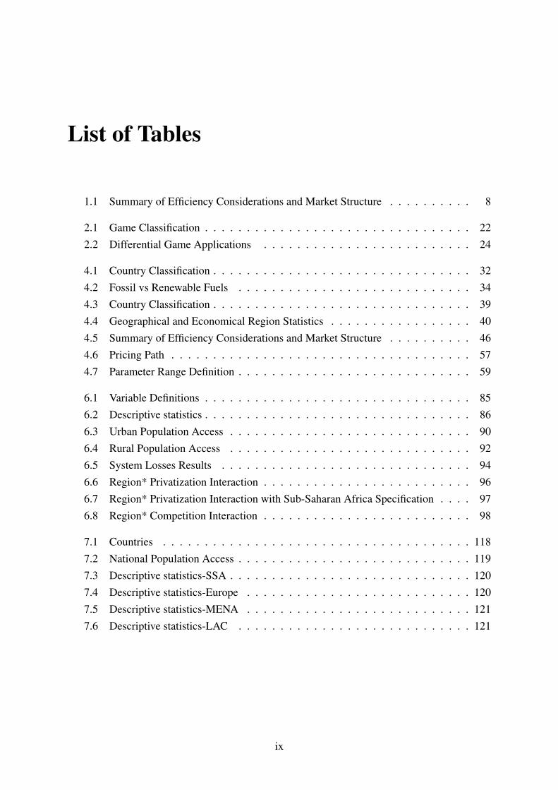
List of Tables

1.1 Summary of Efficiency Considerations and Market Structure . . . . . . . . . . 8

2.1 Game Classification . . . . . . . . . . . . . . . . . . . . . . . . . . . . . . . . 222.2 Differential Game Applications . . . . . . . . . . . . . . . . . . . . . . . . . 24

4.1 Country Classification . . . . . . . . . . . . . . . . . . . . . . . . . . . . . . . 324.2 Fossil vs Renewable Fuels . . . . . . . . . . . . . . . . . . . . . . . . . . . . 344.3 Country Classification . . . . . . . . . . . . . . . . . . . . . . . . . . . . . . . 394.4 Geographical and Economical Region Statistics . . . . . . . . . . . . . . . . . 404.5 Summary of Efficiency Considerations and Market Structure . . . . . . . . . . 464.6 Pricing Path . . . . . . . . . . . . . . . . . . . . . . . . . . . . . . . . . . . . 574.7 Parameter Range Definition . . . . . . . . . . . . . . . . . . . . . . . . . . . . 59

6.1 Variable Definitions . . . . . . . . . . . . . . . . . . . . . . . . . . . . . . . . 856.2 Descriptive statistics . . . . . . . . . . . . . . . . . . . . . . . . . . . . . . . . 866.3 Urban Population Access . . . . . . . . . . . . . . . . . . . . . . . . . . . . . 906.4 Rural Population Access . . . . . . . . . . . . . . . . . . . . . . . . . . . . . 926.5 System Losses Results . . . . . . . . . . . . . . . . . . . . . . . . . . . . . . 946.6 Region* Privatization Interaction . . . . . . . . . . . . . . . . . . . . . . . . . 966.7 Region* Privatization Interaction with Sub-Saharan Africa Specification . . . . 976.8 Region* Competition Interaction . . . . . . . . . . . . . . . . . . . . . . . . . 98

7.1 Countries . . . . . . . . . . . . . . . . . . . . . . . . . . . . . . . . . . . . . 1187.2 National Population Access . . . . . . . . . . . . . . . . . . . . . . . . . . . . 1197.3 Descriptive statistics-SSA . . . . . . . . . . . . . . . . . . . . . . . . . . . . . 1207.4 Descriptive statistics-Europe . . . . . . . . . . . . . . . . . . . . . . . . . . . 1207.5 Descriptive statistics-MENA . . . . . . . . . . . . . . . . . . . . . . . . . . . 1217.6 Descriptive statistics-LAC . . . . . . . . . . . . . . . . . . . . . . . . . . . . 121

ix

Acknowledgements

I must first thank my advisors, Dr. Janis Terpenny and Dr. Johannes Fedderke, for their guid-ance and for allowing me the opportunity to conduct research with them and affording me theintellectual freedom to explore and express my ideas. I would like to thank the members of mythesis committee, Dr.Shanbhag, Dr. Chen and Dr. Fang, for contributing their expertise andinsight along the way. Many thanks to all the teachers l have had over the years, this is theculmination of all the guidance and wisdom you imparted on me.

I also give thanks to my family. Without their support this achievement would not be possible.This is for you too. Vabereki vangu nemhuri yedu ndinokutendai nerudo rwenyu nekurudziroyenyu parwendo rwangu. Seke mutema vangu aihwa basa ramakabata iguru. Makarovedzakukosha kwechikoro kubva pazera duku, nzira iyoyo ndiyo yatisvitsa pano nhasi. Chihera ndi-nokutenda nekuzvinyima kwenyu kuti ini nehnzvadzi dzangu tiwane nhaka youpenyu, inovandiyo nhaka yedzidzo. Handikanganwe nemiwo Chikonamombe, zvaisava nyore kushandiramhuri yakakura kudaro. Asi imi maishingaira kuti tive neraramo yakanaka, uyezve tiendekuzvikoro zvakatipa mukana mukuru wekubudirira muzvidzidzo zvedu. Manyuka ndinoku-tendai zvakapfurikidza. Handikanganwe nemiwo ana maromo vangu, Constance Matenga,Agenia Matenga,Lillian Matenga, Rumbidzai Matenga na Yevai Matenga, mese ndinokutendainerudo rwenyu.

Baba na Mai Chigume handigone kutenda zvakakwana. Rudo rwamunogoverana neni rwunondikoshera.VaChigume ndinokutendai nekuve muenzaniso wakanaka uyezve kuve chipangamazano changu.Vatete vangu Edeline Chigume ndinokutendai nekuve amai, baba na tete panguva dzakafanira.Mwari arambe achikuropafadzai pane zvese zvamunoita.

MntakaKhumalo, umzukulu kaMatshobane, unkulunkulu akuphe izibusiso ezingapheliyo

I wish to express my deep gratitude to my PSU family; Dr. Kimberly Ann Harris, Toyosi Ade-mujimi, Adam Meyers, Cody Hohl, Dr. Tawanda Zimudzi, Dr. Beatrice Abiero and ChaitanyaKaul. You made this journey exciting and fulfilling. I would like to thank my colleagues, col-laborators and good friends in the Smart Systems research group, Amol Kulkarni, Dr.ConnorJennings and Yupeng Wei, I am forever grateful for your generous feedback and always en-

x

couraging me along the way. Thank you!

xi

Kuna amai vangu Elizabeth Matenga na baba vangu Lazarus Matenga.

xii

Chapter 1

Introduction

1.1 Background

1.1.1 Regulated Electricity Markets

Regulated markets generally have a single utility provider that has monopoly power over theentire electricity supply chain i.e generation,trading, transmission, distribution, and retail. His-torically, all electricity markets were regulated markets. However this has since changed as themajority of electricity markets today are deregulated markets. Even under competitive mar-kets, there still exists some form of regulation. Regulation is implemented as a means to: (1)to set a reasonable rate of return for the investors and (2) to attract investment in order to sat-isfy consumer demand. The regulatory authority can be the government, local municipality,or a private board. In electricity markets, there exist several ways to achieve the goals setby the regulator. These methods include (1) Rate-of-Return(ROR) and (2) Perfomance-BasedRatemaking(PBR).

Under ROR method, the regulator must conduct thorough research in order to determine thefollowing; (1) Costs incurred by the utility supplier, (2) Value of investment, and (3) Appro-priate rate of return on the invested capital. The process of gathering enough information todetermine the steps above can be cost intensive to the regulator. The PBR method introduces amechanism that attempts to reduce this cost of information gathering [1]. [1] identifies the fol-lowing as the main policy variables that can be implemented to achieve the goals of electricityregulation:

• Regulated Tariffs- The regulator gives the utility the total revenue it should get fromserving its current customers. The utility provider can determine the price it can set toachieve this revenue. In an ideal setting, this price will be set at the marginal cost ofproviding electricity to each customer.

• Allowed investment- The regulator sets the allowable levels of capital in each of the

1

stages of the electricity chain; generation, transmission, and distribution.

• Access rules- This is a policy instrument that involves the entry and exit of the marketplayers.

• Quality of service requirement- It is difficult to measure quality in many markets, how-ever , Rothwell and Gomez [1] generally describes the following as the measures ofquality in electricity markets ; (1) reliability, (2) power outages and voltage disturbances,and (3) consumer satisfaction.

Regulatory Process

The goal of the regulator is to create a regulatory process that maintains an arrangement be-tween the regulator and the market players that maximizes social welfare by reducing socialcosts incurred by the public and maximizing social benefits from the participation of the marketplayers in the market. There is evidence that supports that in some cases government ownershipwith government oversight maximizes welfare. This condition is satisfied when the governmentoperates in an efficient way. Most governments in the developing world lack the effective regu-latory frameworks. This might be due to high levels of corruption or political instability. Undersuch conditions and the uncertainty of regulatory directives, the return value to the investorcan be substantially diminished [81]. Therefore, the likelihood of government ownership withgovernment oversight maximizing social welfare in developing countries is minimal. However,there is strong evidence that supports that private ownership with independent regulation ismore equipped to minimize social cost of electricity provision thus maximizing social welfarebetter than the government ownership with government regulation framework. The former ismore feasible in the deregulated markets, and therefore the developing markets can achievethese levels of efficiency by deregulating their electricity markets. Rothwell and Gomez [1]establish that it is important to ensure independence between branches of government and theregulator as this minimizes the political influence on the prices set by the utilities. It is alsoimportant to maintain independence between the regulator and the the utility to reduce thechances of regulations that maximize utility profits at the expense of the consumers. In fact,insurance of independence is so important that some countries have conflict of interests legis-lation to ensure the highest level of independence is attained [1]. This regulatory frameworkcan be implemented in the electricity markets in the form of ROR and the PBR.

Rate of Return Regulation

The rate of return regulation involves determining the allowed costs and investments by theutility and then setting up an allowed level of return such that the utility appropriate earningson its investment. Rothwell and Gomez [1] summarizes this process in three points;

2

1. The utility or the regulator argues that the tariff is too low/high because the cost allowanceor allowed rate of return is too low/high.

2. Both parties negotiate a new set of expenses allowed and the new rate of return.

3. Tariffs are adjusted to meet the new rate of return allowed by the regulator.

The rate of return has its advantages especially in terms of investor confidence in having a fairopportunity to receive appropriate profits for investments. However, it is only sustainable in anon competitive market. It also provides little to no incentive to the utility to operate efficiently.In times of high inflation, the rate evaluation has to occur frequently and this proves to be costlyin the long run. The rate of return regulations provides a means for companies to shift costsfrom competitive markets to non-competitive markets [29].

Perfomance Based RateMaking

The perfomance based ratemaking works as follows. The regulator uses the utility’s observedand projected costs to set up the initial price. This price is the baseline for the utilities for aset period of time. This time period is usually set as a 12 month period. Also, the regulatorsets incentives for the utility to reduce costs , improve efficiency or increase benefits to theconsumers. Perfomance metrics are put in place in order to discourage utilities from creatingsavings by cutting on safety, reliability and quality. A framework to share the resultant savingsis established between the regulator and the utilities. The provision of the incentives is themain difference between ROR nad PBR .The performance based ratemaking is designed on thebasis of information asymmetry between the regulated utilities and regulators. It emphasizesratemaking methods that will lead to performance without excessive regulatory oversight. His-torically, it has been used as a means to decouple the link between the utility’s revenue and thevolume of its sales. This is achieved through an automatic mechanism that adjusts rates basedon the over-or-under recovery of the target revenues [29]. Some of the main objectives of PBRinclude , reduced costs for the utility, improved quality of service, appropriate allocation ofrewards and risk between the utility and the consumers. The main advantages of PBR can besummarized as follows:

1. Improved resource efficiency,

2. Reduced administrative and regulatory costs,

3. Improved allocative efficiency,

4. Easier introduction of new services, and

5. Compatibility with transition to competition.

3

While there are a number of benefits of the PBR methods. there are a number of drawbacksfrom using this regulating method. The main disadvantages of PBR are as follows:

1. Reduced quality of service,

2. Questionable efficiency benefits,

3. Questionable administrative costs savings,

4. Limited ability to incorporate environmental and social goals, and

5. Undesirable equity impacts.

While the PBR method gives incentive to utility companies to reduce costs and increasebenefits to the consumers which can be similar to a competitive market, it is only a transitionto competitive markets. This mechanism also requires the regulator to carefully design the in-centive structure, performance metrics in order to induce the desired benefits. The performancemetrics set needs to be measurable in order for the regulator to evaluate each utility. This canprove to be difficult for the regulator. It is also difficult to generalize the PBR methods in thepresence of multiple players and different technologies.

The ROR and PBR work best in regulating a monopoly utility. These methods are not effectivein the case competitive markets. It is still important for the regulator to develop a strategy thatcan be used to monitor the welfare of consumers in a competitive market.

1.1.2 Public Choice Theory of Regulation

The theory of public interest of regulation carries the assumption that regulation serves the in-terests of the consumers. In this case it is the assumptions that the government or the privateregulatory authority serves the interest of the consumers by implementing policies the improveconsumer welfare, protects the environment by inducing a restriction on the actions by the firmsthat can reduce consumer welfare or damage the environment. This assumption is challengedby the public choice theory of regulation. The public choice of regulation claims that all indi-viduals are driven by self interest [3] i.e all decision making individuals be it public servants orindependent individuals. It is also a theory that put forwards that governments can also fail.

The premise of the public theory of regulation suggests that not all regulatory processeshave the objective of maximizing social welfare. It suggests that regulatory agencies throughits workers cannot be exempted from the rational axioms that a decision maker will alwaybehave as if he or she is maximizing an individual utility. This notion of self interest at theexpense of public interest is exacerbated in developing countries where the levels of corruptionare high. The majority of developing countries have a corruption perception index (CPI) < 40[5]. The averages of the worst performing regions are as follows; Sub-Saharan Africa (32),

4

East Europe and Central Asia (34). Corruption is not limited to the least developed regions,however its impact on growth is greater in developing countries.

Public choice theory implies that the regulatory process is one in which different playersseek to maximize their on benefits. The firms can use the regulatory process to maintain amonopolistic market structure, while consumers will use the regulatory process as a way oflowering prices at the expense of the firms providing the service. The regulatory authoritiescan also seek personal gains such as monetary incentives or political incentives therefore im-plementing policies that cater to these needs at the expense of the public interest. Public policytheory of regulation highlights the importance of setting up structures that aim to remedy thisproblem. This can be achieved by creating a number of agencies that monitor each other in acycle. This guarantees that no one agency has absolute power.

1.1.3 Deregulated(Competitive) Electricity Markets

In contrast to the regulated market, deregulated markets have multiple utilities that have di-vested ownership of the electricity supply chain. This includes generation, transmission anddistribution. Utilities compete for prices and consumers. In deregulated markets, the utilityhas an incentive to sell power to not only the consumers near the power plant but to extend itsmarket to long distance consumers. Allowing trading of electricity can cause a strain on thetransmission grid designed for local monopolies, however in the case of low network access, theutility has an incentive to build the infrastructure to facilitate expansion. Competition providesan incentive to firms to respond to consumer needs, reduce operational costs, and compete onthe basis of prices. This influences utilities to be innovative in order to gain competitive edgeover peer companies. This edge may be temporary since the other firms will respond accord-ingly. However, it helps the competition with innovation which in turn helps consumers andthe environment. Some of the benefits of electricity deregulations include the following:

• Provision for competition- Deregulation ensures that all companies have an equal oppor-tunity to provide electricity to consumers. Creating a level playing field ensures that noone firm has exclusive right to serving consumers and it also eliminates some barriers toentry.

• Lower prices for consumers- The presence of competition allows the consumers to seekcost competitive alternatives. This results in reduction of costs on the consumers side.

• Improved service reliability - In the presence of a monopoly , consumers cannot switchto a different provider once the monopoly proves to be unreliable. In the presence ofcompetition, utility providers are forced to take into account the possibility of losingcustomers due to poor service reliability. This creates accountability on the part of thefirms.

5

• Environmental benefits - The presence of competition forces the utilities to explore ef-ficient ways of producing electricity in order to lower the costs. This means improvingtechnology, thus reducing environmental damage and the firms reduce the costs of envi-ronmental taxes etc. All these factors result in cleaner generation of energy.

1.1.4 Externalities

One of the resultants of fossil fuel electricity generation is pollution. This is especially true inthermal power plants that use fossil fuels. The burning of fossils fuels emits pollutants suchas S02, CO2, N0x. These gases lead to acid rain and cause different ailments. [60] shows thatair pollution has negative effects on health and contributes to mortality rate, cardiovascular andrespiratory illness. He quantified the impacts of coal operated power plants in South Africato be valued at $ 2.4 billion annually. The cost of the impacts caused by the coal fired plantsaccumulates yearly during the lifetime of the plant. With average lifetimes of nearly 20 yearsfor thermal power plants, the costs on the the population becomes very large [60]. In recentyears there has been a push amongst nations to gradually transition to greener energy sourcesas the consequences of climate change have become more apparent. According to the WorldBank environmental indicators, the world combined released 4.972 metric tons per capita in2014. With the exception of South Africa, African and developing countries emit less C02 fora unit of GDP than the world average. This is a result of the lower levels of industrializationin developing countries and lower levels of electricity access. The level of C02 emissions isdirectly proportional to the levels of electricity demand. Therefore the lower levels of demandin developing and African countries explain the low C02 emissions per capita. Both academicsand policy makers are concerned about the best way to reduce greenhouse effects and minimiz-ing the economic effects that can arise from such action. There is a need to find an efficientway to deal with this issue.

Tradable Permits vs Emission Taxes

On December 10, 1997, 160 countries signed the Kyoto Protocol agreement on limiting emis-sions of greenhouse gases [125]. This set in motion the debate on how to efficiently achievethe reduction in pollution in different economies. Economic literature draws a clear distinctionbetween command and control approaches (CAC) and market-based incentives (MBI), with thelatter being preferred over the former [125]. The high costs of monitoring in the CAC approachmakes it less desirable. Two MBI instruments have been used as a control strategy for greenhouse emission reduction: enviromental taxes and tradable permits have been adopted by dif-ferent countries over the past two decades. The main challenge to policy makers is knowingwhich instrument to adopt and under what conditions will the instrument be more efficient.There is established economic literature that details the efficient conditions to implement eitherthe environmental tax or the tradable permits.

6

Environmental Taxes

Environmental taxes are also known as Pigouvian taxes. This is a tax that is charged on anymarket activity that imposes costs on the society (negative externalities). The intent of this taxis to move the market from an inefficient point to an efficient point where the cost to society islower than the inefficient point. In energy economics, this can be achieved by levying a carbontax on power suppliers. The tax levied on the suppliers needs to be equal to the total damagecaused by the extra unit of emissions. This means that the tax needs to be a true reflectionof the cost to society, therefore the power supplier has an incentive to reduce emissions to thepoint where a unit reduction in emission is equal to the social damage [60]. According to VanHeerden the Pigouvian tax has four effects on an economy [58];

1. taxes result in an increase in production costs in energy intensive industries, thus reducingexport demands of energy intensive goods , making imports a more attractive alternative.This reduces the output in energy intensive trade related sectors. There is also a shift oflabor supply from energy intensive sectors to less energy intensive sectors.

2. Increase revenue collected by the government, however this revenue needs to be dis-tributed in order to avoid a reduction in purchasing power, thus resulting in a decreasehousehold consumption.

3. Cause a decrease in GDP. This is because the tax causes an increase in prices, therebyincreasing inflation. The increase in costs reduces consumption, therefore reducing out-put levels by industries. This results in a decrease in the GDP. This directly affect theunskilled workers whose wage-price ratio goes down as inflation increases.

4. Cause substitution from energy and energy rich commodities to sectors with low energyconsumptions. This reduces demand in energy, therefore resulting in a decrease in green-house gas emissions.

Setting up an efficient tax regime requires the regulator to have a lot of information about theutility company. The regulator needs information about the marginal abatement costs (MAC)and marginal benefits cost (MBC) of the utility. Without this knowledge it becomes challengingfor the regulator to set up a tax level that will achieve the efficient levels of emissions.

Tradable permits

The Tradable permit system requires the regulator to investigate and set a cap on the levelsof pollution allowed for a specific industry. In this case it is the levels of pollution allowedfor electricity generation. Once the pollution cap is established, the regulator issues permitsthat amounts to the cap limit e.g. a cap of 3 000 000 tonnes of C02 will require 3 000 000permits. These permits are either distributed to the participating firms or sold in a blind auction

7

(highest bidder wins). No firm is allowed to emit pollution without acquiring the equivalentnumber of permits. After acquiring the permits, a firm can buy or sell permits to/from otherfirms. Tradable permits can induce innovation and development as firms seek ways to minimizecosts. A potential shortfall of tradable permits is in dealing with market power. Koustaal [?]andXepapadeas[75] separately established that firms when firms behave as price setters , the gainsof tradable permits are lost . The following table summarizes the main finding of the discussionprovided by Norregaard and Reppelin-Hill [125].

Table 1.1: Summary of Efficiency Considerations and Market Structure

Market Structure Emission Tax Tradable Permits

Perfect Competi-tion

Efficient Efficient

Noncompetitivemarket in theoutput market

Efficient can beachieved by suit-ably adjusting thePigouvian tax butonly if firms areall identical

Inefficient but lit-erature suggeststhat efficiencylosses may besmaller thanunder an emis-sion tax(whenfirms have dif-ferent pollutiontechnologies).

Noncompetitivemarket structurein the permitsmarket

N.A Inefficient

Source = Norregaard and Repellin-Hill 2000

The importance of privatization is supported by the inefficient levels that are achieved byboth the emissions tax and tradable permits in a monopolistic market [47]. By introducingcompetition, the market becomes efficient under both the emission tax or the tradable permits.It is important to note that the environmental tax achieves a social optimum [68] when thefirms causing pollution are identical, i.e, use similar technology for electricity production. Inthe case of dissimilar technologies, only the firm specific environmental tax achieves the socialoptimum [68].

1.1.5 Current State of Electricity Markets in Developing Economies

It is a challenge for policy makers to design an efficient market structure for a region thatfaces deficiencies in utility coverage, service backlogs of grid repairs or expansion, unique so-cioeconomic characteristics, unique institutional endowments and weak economic regulatory

8

mechanisms [81]. Economic regulation of utilities include issues such as pricing, cost of ser-vice, investments , quality (this includes service obligations and set service standard) and rateof returns on assets [4]. Most countries in the developing world have a monopolistic designfor power markets. This can be through government policy or a superior utility provider thatimposes a monopoly. The lack of competition, brings about challenges in the continuity ofservice delivery and the quality of services provided. It also provides challenges in establishingeconomically efficient prices for the utility. Government regulation can make it difficult forthe utility provider to make profitable investments in enlarging its network. Also, the utilityprovider can charge exorbitant prices because of its dominant control on the sector. These chal-lenges make it difficult for consumers in these markets to have access to reliable and efficientservices. This in turn affects the economic development of these countries since power supplyplays a critical role in the efficient operation of industry and service systems. All challengesraised in this section can be explored with focused research on each challenge. However, thisdissertation focuses on understanding the pricing dynamics due to entry into the market by acompetitive firm. The World Bank (2008) showed that , in Sub-Saharan Africa, 26% of thepopulation has access to electricity, 1% to fixed telephony, 14% to mobile , 60% to water, and34% to rural transport[73].

Most Sub-Saharan African countries like Zimbabwe, Angola and South Africa heavily de-pend on fossil fuels for electricity generation. Mainly because it is cheaper and fossils arereadily available in most of these countries. However, fossils such as coal lead to large emis-sions of Carbon-dioxide and Sulphur dioxide. These lead to acid rain, which affects agriculturalproduction. Most of Sub-Saharan Africa heavily relies on subsistence and commercial farmingfor income generation on a household and national level respectively. This leads to a reductionin social welfare and quality of life. The calls for a cleaner earth and the advancements intechnologies used to extract and use renewable energy sources has changed energy economics.There is a need for an active investigation into how to efficiently incorporate different sourcesof energy on the same grid to increases consumer utility. The research on electricity marketsis therefore important in addressing such issues especially given the World Bank’s target of92% electrification worldwide by 2030 [73]. For such rates of electrification to be achieved,there is a high need to understand methods to boost investments for electrification in develop-ing countries since these lag behind the rest of the world in terms of electricity access. Oftenthe regulatory uncertainties in most developing countries have been cited as one of the manycauses for under investment in infrastructure development [81]. However, research in optimalinvesting can be used by investors to minimize risk and still be profitable in uncertain mar-kets. Therefore, the use of both optimization models and economic techniques can be highlyvaluable in helping increase investment in infrastructure development projects in developingcountries.

9

1.1.6 Motivation and Significance

The presence of adequate and efficient infrastructure is widely recognized as an importantfactor in the quest for economic growth. This recognition comes from both policy makers andacademics who work on understanding the role of infrastructure in economic growth [9, 114,11]. While most developing countries face the problem of infrastructure development, sub-Saharan Africa is consistently ranked bottom in terms of infrastructure performance. There area number of studies that focus on either forecasting the infrastructural needs or comparativeunderstanding of the effects of infrastructure deficiencies in Sub-Saharan Africa. [44] use aneconometric approach in estimating the demand for electricity and telephony, and used this toproject the dollar investment needs in electricity and telephony for South Africa . This approachcan be extended to any developing country. Luis Serven at the WBG has done extensive workon providing empirical evaluations on the effects of infrastructure development to the growthof an economy and income distribution [13]. While these studies provide useful information topolicy makers, they do not address the question of how to meet these needs in the long term.While this project does provide a framework that can be used to meet the infrastructural needsof the future, it provides an analytically tractable long term pricing path for firms that seek tomaximize long term profits and network size. It also provides a policy framework for policymakers environmental and social goals.

The dependence of productivity and social welfare on the access of regular and uninter-rupted electricity supply are well established. Both factors contribute to economic developmentand environmental sustainability, therefore uninterrupted access to electricity supply is impor-tant for economic growth. The research methods applied on electricity markets need not belimited to just electricity markets. These methods can be extended to any infrastructural needsfor developing and developed countries. Optimal control theory and differential game theoryare applicable in scenarios that require finite or infinite horizon planning and the existence ofplayers interacting strategically.

As the demand for electricity increases and the access rates improve, the amount of green-house gas emitted into the atmosphere increases. It becomes the responsibility of policy makersto craft policies that improves the investments into electricity while minimizing the amount ofpollution from electricity generation. These types of problems have been studied in literatureas the Social Planners Problem.

This dissertation focuses on the implementation of optimization methods and economictheory on designing an efficient market structure. Specifically, the main focus is on developingcountries whose energy markets are undergoing privatization. The goal is to formulate the de-sign of an optimal pricing path for new market players whose objective is to maximize long-runprofits by optimizing network size. The market entrants face a state utility that maximizes longrun profits. In other words, the pricing structure of the incumbent is deterministic. Entrant play-ers can use this analytically tractable framework for optimal pricing and profit maximization.

10

This framework can also be useful in informing market players on decisions on infrastructureinvestments. The framework provides a set-up of market structures that allows the fulfillmentof infrastructural needs of the future by empowering both the investor and the policy makers.The aim is to help accelerate electricity infrastructure development in these countries. It is alsoimportant to quantify the benefits of establishing competitive markets and compare the perfor-mance of electricity markets in different economic regions. Using an econometric approach,this dissertation provides an approach to measure the effects of privatization and competition.This provides an objective measure that can be used to shape economic policies in developingeconomies.

1.1.7 Research Purpose and Objective

The goal of this dissertation is to use optimal control theory and differential games to analyzethe electricity markets in developing countries. The main contribution will be providing aframework for introducing competition in the electricity markets of developing countries. Thiswork will also add to the already existing literature of environmental taxes as an instrument toreducing pollution. To date, there is little or no literature that models environmental taxes in adifferential game structure for electricity markets in developing countries nor the introductionof competition by the entry of a competitive firm that seeks to maintain its market presenceby implementing profit maximizing strategies. There exists a clear distinction between thedeveloped countries’ electricity markets and developing countries’ markets. These differencescan be summarized as:

• Nature of market design( Monopolistic vs Competitive ),

• Level of electricity access,

• Government efficiency, and

• Infrastructure development.

The focus on competitive markets stems from the possible benefits that these markets provide;the competitive pressure can result in lower prices, efficient technology and increase in levelsof electricity access. These direct consequences of competition are the targets of policy makersin developing and developed electricity markets. The following subsections summarize theresearch questions explored. Listed below, the research questions include :

• Can firms achieve optimal pricing paths in privatized underdeveloped networks,

• What is the optimal taxing strategy to increase competitiveness of green utilities,

• Can subsidies minimize entry deterrence in the presence of a dynamic pricing cap, and

• Are the effects of privatization and competition in electricity markets measurable.

.

11

1.2 Organization of Dissertation

The first chapter provided the background and the significance of continued research in thedesign of electricity markets in developing countries to improve infrastructure development,access of electricity, environmental protection policies and pricing methods. It also providesthe research purpose, motivation,and research contributions. The remainder of the dissertationis organized into seven chapters, as outlined below;

Chapter 2: Literature Review

This chapter reviews the literature related to the focus of this study, this includes (1) pricing

methods that are employed in the electricity markets of developing countries (2) Optimal con-

trol theory and its applications to market share competition (3) Game theory methods, specifi-

cally the extension of optimal control theory to differential games.

Chapter 3: Research Methods

This provides the methods that are used in analyzing the proposed research questions. This

includes methods used in solving differential games i.e Open Loop Nash Equilibrium, Open

Loop Stackelberg Equilibrium, Markovian Nash Equilibrium and Non-Markovian Nash Equi-

librium

Chapter 4: Pricing Dynamics of Electricity in Privatized Competitive Markets with Devel-oping Networks

This chapter provides an analysis of the pricing path that is followed by a profit maximiz-

ing state utility that is facing a serious entrant firm that is also maximizing its long run profits.

The pricing path will be influenced by the parameters used in modeling the cost function and

the state dynamics.

Chapter 5: Optimal Taxing Strategy to Increase Competitiveness of Green Utility Suppliers:A Theoretical Framework

This chapter provides an analysis on the use of a taxing strategy in order to help green utilities

becomes sustainable market players. Green utilities face high investments cost that makes them

less competitive in terms of price relative to conventional energy utilities. A policy maker that

Chapter 6: Measuring the effects of Competition and Privatization in Electricity Markets: AnEconometric Approach

12

The focus of this chapter is the validation of the models suggested in the previous chapters

by using real world data. This data will come from developing countries that have made the

transition from regulated market structure to deregulated market.

Chapter 7: Conclusions and Future Work

This chapter includes the summary of the research analysis in the previous chapters, contri-

butions and the advantages of the proposed methods. It also provides a description of areas for

future research is discussed. This consists of areas where the research can be expanded either

by using newer methods or an extension of some of the models used in this dissertation.

13

Chapter 2

Literature Review

This chapter provides a review of the literature that is relevant and closely related to the topicsdiscussed in this research. There is a thorough discussion on the evolution of the methods ofpricing electricity in regulated or semi-deregulated markets.The review also provides an insighton the implications of these methods to economic growth, social welfare and policy formulationin these markets. Finally, this chapter provides a discussion of the methods used in formulatingand analyzing pricing models in a deregulated market. Specifically, it provides an overview ofoptimal control theory and the extension of this theory to differential games using the principlesof game theory.

2.1 Pricing Electricity

Pricing public utilities is a challenge especially in developing countries. The goal of pricing isto allow efficient allocation of resources in the system. The firms are interested in profitabilitywhile government/ policy makers are interested in social policy and political objectives . Itis difficult to find a balance between the two different objectives, since developing countriesoften lack the necessary conditions to achieve an efficient market where P = MC. In manydeveloping countries, there exist state owned utilities that will implement prices, where P<MC

for political reasons. The following methods have been used in the past to determine the pricesof electricity in the developing countries.

• Cost Recovery Pricing- This requires the setting of a price that allows the service providerto recover its investments costs and also gain an acceptable return on investment. This canalso include depreciation costs. This approach is often used by state controlled utilities insituations where the value of assets is significantly greater than the additional investmentsrequired in future periods. A regulatory board determines a fair return bounds on theinvestments by considering both social and political objectives. It is easier to calculatethe cost of production once a fair rate of return has been determined The price allowed

14

becomes;P = µ(AC) 1≤ µ ≤ b

Where AC = average cost of energy generation, µ = allowable mark up percentage and b

= the bounds on the allowable mark up.A market that employs this pricing method creates a strong barrier to the introduction ofcompetition. It also does not reward for efficiency and performance since the return is setbased on the level of fixed assets of the utility provider. The lack of performance basedrewards leads to the disadvantages similar to that of a monopoly discussed previously[74].

• Marginal Cost Pricing- Prices of the electricity are set as equal to the marginal cost in-curred by the utility to provide electricity to each additional consumer. The limitation ofmarginal cost pricing is that it does not take into account capital cost in the short run [64].Energy investments are long term investments, therefore marginal costs should includethe costs of expanding and capacity or improving technologies used in the generation ofpower.

• Opportunity Cost Pricing-The utility analyzes how much it would charge for its serviceif it was located in a different country. This method provides a good check for policymakers if the markets chosen have similar characteristics to the market under study. Sincemost countries do not observe the same market conditions this method does not providea good check for internal pricing. For example, Zimbabwe and South Africa have someof the world largest coal reserves , but there is a large disparity between the level of coalproduction in both countries. This means that using the opportunity cost pricing methodwith each neighbor as a reference point is not an effective pricing benchmark for eithercountry. The country specific differences means that the prices charged do not alwaysreflect opportunity cost for a player in a different market [74].

• Market Pricing- This pricing method is used when there are multiple players in the mar-ket. The price converges to an optimal price for the allocation of resources in the market.Economic theory shows that this is the most efficient method of pricing. However, marketpricing does not always converge to affordable prices for consumers[74]. This poses aproblem for policy makers in developing countries whose objective is to provide a struc-ture for regular and affordable electricity services to the consumers. However, it reflectsscarcity of resources which should be incorporated into policy making.

2.2 Optimal Control and Differential Nash Games

Optimal Control is the process of determining control and state trajectories for a dynamic sys-tem over a period of time to satisfy a given objective function i.e. minimization or maximiza-

15

tion. Optimal control theory was developed by Russian mathematicians. One of the maincontributors to optimal control theory is Pontryagin who developed the Maximum Principle.Economists like Dorfman [18] extended optimal control theory to economic applications. Op-timal control optimization has the following advantages;

• Allows long run planning,

• Allows flexibility, and

• It is commonly used in several industries such as electricity, transport, retail and enter-tainment.

The following is a general optimal control problem formulation as defined in [17] ;

maxu(t)

J =∫ T

0F(x(t),u(t), t)dt +S[x(T ),T ]

s.t

xi(t) = fi(x(t),u(t), t) i = 1, ....,n; (Transition Equation)

xi(0) = xi0 i = 1, ....,n; (Initial Conditions)

xi(T )≥ 0 i = 1, ....,n; (Terminal Conditions)

u(t) ∈ℜn (Feasible set)

Where,

x(t) = is an n-vector of state variables(xi(t)). The state variables describes the state of thesystem at any given point in time. We have dxi

dt = xi

u(t)= is an n-vector of control variables. The optimization problem is solved over these vari-ables.F(.) is the objective function.f (.) is the transition function for each state variable.

The Pontryagin maximum principle is used to solve the optimization problem by defining aHamiltonian function,H. The following is the Pontryagin’s theorem as presented in [17]

Theorem 1 For x∗(t) and u∗(t) to be optimal for (1), it is necessary that ∃ a constant λ0 and

continuous functions Λ(t) = (λ1(t), ...,λn(t)), where ∀ 0≤ t ≤ T we have λ0 6= 0 and Λ(t) 6= 0such that ∀ 0≤ t ≤ T ;

H(x∗(t),u,Λ(t), t)≤ H(x∗(t),u∗(t),Λ(t), t)

16

where the Hamiltonian function H is defined as;

H(x,u,Λ, t) = λ0F(x,u, t)+N

∑i=1

λi fi(x,u, t)

with the exception at the points of discontinuity of u∗(t),

∂H(.)

∂xi=−λi(t), i = 1, ..,n.

Furthermore , λ0 = 0 or λ0 = 1 and, finally , the following transversality conditions are

satisfied;

λi(T )≥ 0, λi(T )x∗i (T ) = 0, i = 1, ...,n.

The Hamiltonian defined above has to be concave in x and u for a maximization problem, thenecessary conditions for a maximum are :

∂H(.)

∂ui= 0, i = 1, ..,n;

∂H(.)

∂xi=−λi(t), i = 1, ..,n.

∂H(.)

∂λi= xi(t), i = 1, ..,n.

λi(T )≥ 0, λi(T )x∗i (T ) = 0, i = 1, ...,n.

The optimization problem above may include other transition equations, we have;

maxu(t)

J =∫ T

0F(x(t),u(t), t)dt +S[x(T ),T ].

s.t

xi(t) = fi(x(t),u(t), t) i = 1, ....,n;

si(t) = si(x(t),u(t), t) i = 1, ....,n;

xi(0) = xi0 i = 1, ....,n;

xi(T )≥ 0 i = 1, ....,n;

u(t) ∈ℜn

We define the present value Hamiltonian equation;

H(x,u,Λ,Ω, t) = λ0F(x,u, t)+N

∑i=1

λi fi(x,u, t)+N

∑i=1

ωisi(x,u, t)

17

The Hamiltonian defined above has to be concave in x and u for a maximization problem , thenecessary conditions for a maximum are :

∂H(.)

∂ui= 0, i = 1, ..,n;

∂H(.)

∂xi=−λi(t), i = 1, ..,n.

∂H(.)

∂ si=−ωi(t), i = 1, ..,n.

∂H(.)

∂ωi= si(t), i = 1, ..,n.

∂H(.)

∂λi= xi(t), i = 1, ..,n.

λi(T )≥ 0, λi(T )x∗i (T ) = 0, i = 1, ...,n.

The concavity of the Hamiltonian function can be tested by checking the definiteness of theHessian matrix. The Hessian matrix is defined as follows;

Hi =

[Hxiui

]∀xi,ui i = 1, ...,n

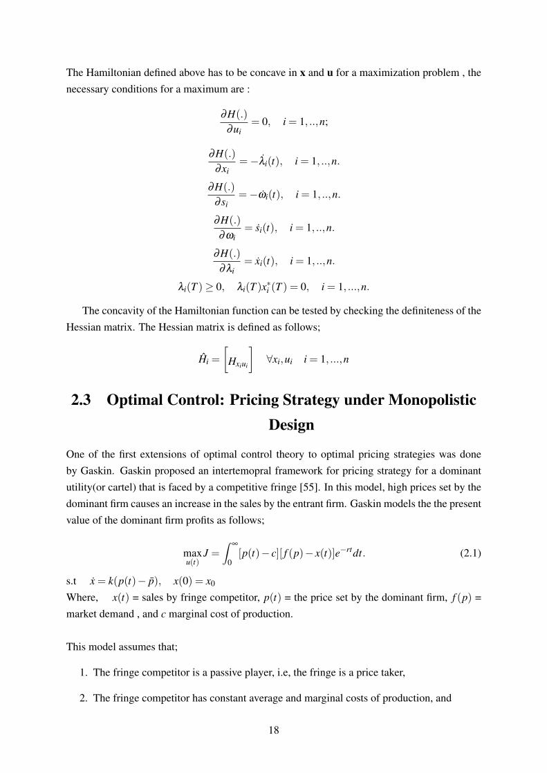
2.3 Optimal Control: Pricing Strategy under MonopolisticDesign

One of the first extensions of optimal control theory to optimal pricing strategies was doneby Gaskin. Gaskin proposed an intertemopral framework for pricing strategy for a dominantutility(or cartel) that is faced by a competitive fringe [55]. In this model, high prices set by thedominant firm causes an increase in the sales by the entrant firm. Gaskin models the the presentvalue of the dominant firm profits as follows;

maxu(t)

J =∫

∞

0[p(t)− c][ f (p)− x(t)]e−rtdt. (2.1)

s.t x = k(p(t)− p), x(0) = x0

Where, x(t) = sales by fringe competitor, p(t) = the price set by the dominant firm, f (p) =market demand , and c marginal cost of production.

This model assumes that;

1. The fringe competitor is a passive player, i.e, the fringe is a price taker,

2. The fringe competitor has constant average and marginal costs of production, and

18

3. The dominant utility has a cost advantage.

Extensions of this model for the monopolistic firm in the presence or absence of competitioncan be seen in [24, 25, 26, 27]. The majority of these models have applications in advertisingand supply chain management etc., and these are of marginal concern to the question posedin this dissertation. Chisari and Kessides, also extend the Gaskin Model to model an optimalpricing strategy of an electricity utility firm that is located in a developing country [81]. Theassumption of an underdeveloped network, poor regulatory reforms, electricity theft are allincluded in the model formulation. The following models the present value profit function ofthe dominant utility;

maxp(t)

Π(t) =∫

∞

0e−rt [PN−C(N)]dt (2.2)

s.t N = γ[ξ (N)−P], N(0) = N0

Where ξ (N) = unit cost of the fringe competitor, P(t) = the price set by the dominant firm,N = Network size of the incumbent , and C(N) = Cost of energy production.The unit cost is defined as;

ξ (N) = ξ0 +ξ N

The unit cost of the the fringe utility as the network size of the incumbent increases. Thedependence of the fringe costs on the size of the incumbent’s network size, takes away thestrategic response that can be implemented by the fringe utility rendering the fringe passive.This lack of strategic interaction between the two firms means that the incumbent firm hasa strategic advantage as it can find an optimal pricing path that will drive the fringe out ofthis market and return to monopoly status. The set up in this project introduces a strategicinteraction between firms, so that it is the market that decides the price and each firm canstrategically respond to the market conditions. This response is captured in the equation ofmotion of the optimal problem for each firm. The equation of motion above is adjusted asfollows;

Ni = γ[Pj−Pi], Ni(0) = N0

Each firm controls its price,Pi, therefore can strategically respond to the markets conditions.No firm has a strategic advantage, and the firms compete on technology and efficiency in orderto minimize operational cost, thereby charging lower prices.

The cost function C(N)is defined as;

C(N) = F +aN + c[ρM+(1−ρ)N]2 +φ N2 a > 0, c > 0 F ≥ 0 (21)

Where F are the fixed costs for each utility provider, φ N2 is the adjustment cost in network size[46, 57], and c are the marginal costs.While this cost function captures the costs due to energy production and theft, it needs to be

19

extended to capture the current conditions in which utilities operate under. These extensions,include but are not limited to environmental tax, abatement costs, theft under multiple playersetc., This chapter extends this cost function to include the dynamics between the dominantutility and a competitive firm, it also includes the presence of an environmental tax as a cost tothe firms in the market.This optimal control model assumes that,

1. The fringe competitor is a passive player, i.e. the fringe is a price taker,

2. The fringe is assumed to have increasing marginal cost as the incumbent increases itsnetwork size, and

3. The dominant utility has a cost advantage.

In this case, prices above the unit cost of the fringe competitor by the incumbent utility resultsin the reduction of its network size. Unlike in the Gaskin’s Model, Chisari and Kessides as-sume that the fringe competitor has increasing marginal costs instead of constant average andmarginal costs i.e., as the the network size of the dominant utility increases , the unit costs ofproduction for the competitive fringe increases. Therefore, by setting prices below the fringemarginal cost, the incumbent makes it more difficult for the competitor to stay in the mar-ket. This model provides an analytically tractable framework for analyzing the optimal pricingstrategy for an electricity utility supplier facing a competitive fringe and an underdevelopednetwork.The obvious short fall of all the models described above is the limited consideration of the opti-mal pricing strategy from the perspective of the incumbent firm. It is not satisfactory to assumethat an entrant firm or a fringe does not seek an optimal pricing strategy. This is of particularconcern when moving from a fringe supplier to a serious market entrant that is likely to provesustainable in terms of presence. This criticism of the Gaskin model is summarized by Gilbert[56] as follows; ”A main criticism of Gaskins’ model is that entry is not an equilibrium process.The entry equation is not the result of optimizing decisions by a pool of potential entrants, butis specified exogenously in the model. The incumbent firm (or cartel) is presumed to act ratio-nally, choosing a price policy to maximize present value profits. But there is no correspondingmaximization problem for the firms that make up the flow of entry into the industry. Firms arenot symmetric in Gaskin’s model in their degree of rationality. Only the incumbent firm(s) canboast an identity in the Gaskin’s model. Entrants are relegated to a nameless component of anoutput flow.”

In order to address the criticism of the Gaskin Model, it is necessary to move from a fringecompetitor to a serious entrant firm that is considered as a profit maximizing firm. This re-quires models that also model the objective function of the fringe competitor under a specifiedcontrol. The following section discusses such models in detail.

20

2.4 Differential Nash Games: Pricing Strategy underCompetition

In order to address the criticism of the Gaskin Model, where the entrant firm is treated as a pricetaking player, there is a need to model the entrant firm as a strategic firm. This requires the mod-eling of the entrant firm’s problem as an optimal control problem. Modeling the entrant firm asa strategic player induces strategic interaction between the entrant and the dominant firm. Thegoal for each firm is to establish an optimal strategy to achieve its own objective function in thepresence of another firm that is also seeking an optimal strategy to achieve its objective. GameTheory provides a theoretical basis of understanding strategic interactions between differentdecision makers or players. In the context of this research, decision maker or players refers tothe entrant firm , dominant firm or policy maker and all the players interact strategically andare assumed to be rational.

A game is defined as dynamic, if the order in which strategies are implemented by the playersis important to the outcome of the game. The game is also defined as non-cooperative if eachplayer solely focuses on achieving its objective which is a conflicting objective to that of theother player. The theory of differential games is derived from optimal control theory and gametheory. Differential games have the following characteristic [32];

• Interdependence: i.e, the decision by a single player influences the achievement of theobjective by the player and the other players involved,

• Strategic : All the players are assumed to be rational, i.e, they consider the influenceof their actions on their objective function and the actions of other players on their ownobjective function. The actions taken by each player becomes a recursive best responseto the best response of the other players, and

• Time : The objective function is either maximized or minimized as an accumulationfunction over a period of time, this can be a finite or infinite time horizon.

The following table summarizes the classification of games with single or multiple players asin [33];

21

Table 2.1: Game Classification

One Player Multiple Players

Static MathematicalProgramming

(Static) game theory

Dynamic Optimal ControlTheory

Dynamic(and / or dif-ferential) game theory

The literature of the structure of a differential game is well developed. Similar to gametheory, differential games require a well defined structure for an effective analysis of the game.The following sections develop the general set up of a general differential game in the form ofthe objective function, elements of the game and information structure.A differential game is defined as an interaction between a set of N players, N = [1,2, ...,N].Each player i ∈ n, has a vector of control ui(t) ∈ Ui ⊆ ℜm j where Ui is a set of admissiblecontrol values for player i. The control, ui(t) , is also a function of the control of the otherplayers. This creates the strategic interaction between the players involved. Each player at anygiven time,t is in a state x(t) ∈ X ⊆ ℜn where X is the set of admissible states. The rate ofchange of the state variables is determined by the equation of motion, which is a system ofdifferential equations;

x(t) =dxdt

= f (x(t),u(t), t), x(t0) = x0 (2.3)

A payoff function for player i, i ∈ n is defined as follows;

Ji =∫ T

t0gi(x(t),u(t), t)+Si(x(T )) (2.4)

where gi is player i′s instantaneous payoff function and Si is the terminal payoff.It should be noted that the time horizon, T, can either be finite or infinite. The difference be-tween the two is established by the transversality conditions for the problem. The instantaneouspayoff can be discounted for time, this is common in infinite horizon problems. The informa-tion structure is defined as the knowledge that is available to player i when he/she selects ui(t)

at t. The following information structures are used in the analysis of differential games;

• Open Loop: This is a game where the players cannot observe the play of their opponentsbefore they make their own decision.

• Markovian(Feedback): All the players can observe the state variable of the other players

22

and make its own decision based on these observations.

The timing of players decisions also determines the nature of the game. There are two typesof decision making we consider;

• Simultaneous - This means that both players choose their strategies concurrently. Eachplayer solves its own optimal control problem by choosing the best response assumingthe best responses from the other players.

• Sequential - The players choose their optimal strategies in an ordered manner. The play-ers are defined as a ”leader” and a ”follower”. The follower solves its optimal problemfirst similar to the simultaneous case. The sequential differential game with a definedleader and a follower is known as the Stackelberg differential game.

The earliest applications of differential game theory were developed for military applicationsby R. Isaacs in the late 1950 to early 1960s. The applications have since been extended to otherfields such as supply chain, environmental economics, marketing, finance etc.. The follow-ing table gives a summary of some of the applications of differential games and the solutionconcepts that have been used in the literature.

23

Table 2.2: Differential Game Applications

Paper Dynamics Control Simultaneous de-cision

Sequential deci-sion

Solution

Eliashberg andSteinberg(1987)[34]

Seasonal Production rate, Price No Yes OLSE

Desai (1992) [35] Seasonal Production rate, Price No Yes OLSE

Desai (1996) [36] Seasonal Production rate, Price Yes Yes OLNE , OLSE

Jain and Chinta-gunta(2002) [37]

NA dynamics Ad.Effort , Price Yes No OLNE, FNE

Fruchter andMessinger(2003)[38]

General Ad. effort , Price No Yes FSE

Kogan andTapiero(2007a)[39]

General Price, Production rate No Yes OLSE

Kogan andTapiero(2007b)[39]

General Processing rate, Pro-duction rate

No Yes OLSE

Kogan andTapiero(2007c)[39]

General Price, order quantity No Yes OLSE

Kogan andTapiero(2007d)[39]

General Price, order quantity No Yes OLSE

Kogan andTapiero(2007e)[39]

General Price No Yes OLSE

He andSethi(2008)[40]

Bass type Price No Yes OLSE

Fanokoa,Telahigue andZaccour (2010)[41]

General Production policy Yes No FNE

Novak , Fe-ichtinger andLeitmann(2010)[42]

General Resource allocation,rate of attack

Yes Yes OLNE, OLSE

OLSE = Open Loop Stackelberg Equilibrium , 0LNE = Open Loop Nash Equilibrium

FNE = Feedback Nash Equilibrium, FSE = Feedback Stackelberg Equilibrium

24

Chapter 3

Methodology: Solving Differential Games

This chapter presents theoretical definitions of the different equilibriums that can be achievedwhen solving differential games. Each equilibrium is achieved under specific conditions; theseconditions are explicitly stated in each section in this chapter.

3.1 Nash Equilibrium

A Nash solution is defined as a set of N admissible trajectories for (2) i.e.

u1∗,u2∗, ...,uN∗

, These trajectories have the property that;

Ji(u1∗,u2∗, ...,uN∗) = maxui∈Ui

Ji(u1∗,u2∗, ...,u(i−1)∗,ui,u(i+1)∗uN∗) (3.1)

for i = 1,2, ...,N In order to satisfy the necessary conditions of a Nash equilibrium solutionfor non-zero sum differential games, a clear distinction between closed loop controls and openloop controls is needed. This shows that each player chooses the best response given the bestresponse of other firms that knows that other firms are choosing their best responses. Thisbecomes a recursive best response of the best response of the best response and so forth.

3.2 Open Loop Nash Equilibrium

In an open loop equilibrium, each player solves its optimal control problem without observingthe decisions of the other players. The players cannot observe the current state of the system.In this case the players decisions depend on the time , t, of the game and the set of feasiblestrategies available to the player. However each players assumes the best response from theother players. The equilibrium is achieved by recursively considering the best response of thebest response of the best response and so forth for each player. In the electricity market this

25

equilibrium is reached in the case where the players do not observe the current price set by thecompetitor until after the period is over. Since the players only observe the price of the previ-ous period, it can assume that the open loop nash equilibrium will be reached when the currentprices set by the market players is not influenced by the price it set in the previous period, i.e,the prices in each period are independent of each other.

The control n-tuple u∗(.) = (u∗1(.), ....,u∗n(.)) is an open-loop Nash equilibrium at (t0,x0)

if the following holds [32]:

Ji(t0,x0;u∗(.))≥ Ji(t0,x0; [ui(.),u∗−i(.)]), ∀ui(.), i ∈ N (3.2)

where ui(.) is any admissible control for player i and [ui(.),u∗−i(.)] is the n-vector of controlthat is obtained when the i− th component of u∗(.) is replaced by ui.Each player solving the following optimal -control problem;

Ji = maxui(.)

∫ T

t0e−ritgi(x(t), [ui(.),u∗−i(.)], t)dt + e−ritSi(x(T ))dt (3.3)

S.Tx(t) = f (x(t), [ui(.),u∗−i(.)], t), x(t0) = x0

3.3 Markovian Nash Equilibrium

In this case, the players can observe the state variable of the other players involved and makeits own decision based on these observation. In electricity markets each player can have ac-cess to the network size of the all the competitor’s since most utility companies provide thisinformation. The following is the technical definition of the Markovian Nash Equilibrium.

The feedback n-tuple σ∗(.) = (σ1∗, ...,σN∗) is a feedback or Markovian-Nash equilib-rium (MNE) on [0,T ]×X if for each (t0,x0) in [0,T ]×X the following holds [32];

Ji(t0,x0;σ∗(.))≥ Ji(t0,x0; [σi(.),σ

∗−i(.)];), ∀σi(.), i ∈ N (3.4)

where σi(.) is any admissible control for player i and [σi(.),σ∗−i(.)] is the n-vector of control

that is obtained when the i− th component of σ∗(.) is replaced by σi.In this case, define σ∗(t,x∗(t))≡ u∗i (t) where x∗(.) is generated by σ∗ from (t0,x0) and solvesthe following optimal control problem;

Ji = maxui(.)

∫ T

t0e−ritgi(x(t), [ui(t),σ∗−i(t,x(t))], t)dt + e−ritSi(x(T ))dt (3.5)

26

S.Tx(t) = f (x(t), [ui(t),σ∗−i(.)], t), x(t0) = x0

27

Chapter 4

Pricing Dynamics of Electricity inPrivatized Competitive Markets with

Developing Networks

4.1 Introduction

There is a need to develop a theoretical framework to understand the intertemporal strategicinteractions between a profit maximizing incumbent utility supplier facing one or more profitmaximizing entrant utility supplier(s) at the early stages of transitioning from a monopolisticmarket to a competitive market.The majority of economic literature considers the Stackelberg,Betrand and Cournot competition models to determine the steady state prices and quantitylevels in a duopoly or oligopoly market. This is informative when analyzing utilities in analready existing competitive market, it is not sufficient to understand the strategic interactionsbetween an incumbent and an entrant firm at the onset of competition in the market. This paperaddresses this gap in the literature by considering the pricing dynamics of two strategicallyinteracting electricity utilities at the initial stages of competition. Understanding this theoreticalframework is not an urgent matter in developed economies since competition already exists inthese economies albeit at different degrees. However, this is not the case in most developingeconomies where the incumbent utility is often a dominant public monopoly. Thus, the generaltheoretical framework developed in this paper directly applies to developing economies wherethere is a need for a policy framework to encourage competition.

For the greater part of the twentieth century, electricity utilities in most countries operatedas state controlled monopolies. The presence of state controlled monopolies often results inpoor quality of service, low service penetration, and low capacity. These problems are morepronounced in developing countries where there are weaker regulatory mechanisms [81]. Thedeveloping economies also face the problem of low access levels to electricity supply; this isnot the case for developed economies where both the rural and urban populations have 100 %

28

access to electricity.Competition in electricity markets, in theory, should lead to improvement in the efficient

use of resources, in the case of most electricity markets the use of coal and other fossil fuels,improve firms financial performance, improvements in service delivery, and capacity factors.The majority of European and North American markets have liberalized their markets to allowcompetition in the electricity markets. While the efficiency gains from adopting such a mar-ket structure are well documented in the electricity market literature, it is important to ask; Iscompetition in a developing economy different from competition in a developed economy? Itmight be the case that the fundamentals of competition are not different; however , the theo-retical considerations for firms are different in these two markets. As mentioned earlier, themarket in a developing economy poses some challenges to utility suppliers including: (1) ac-quiring optimal market share to maximize long run profits, (2) attracting new consumers thatwere not previously served by any market player and (3) underdeveloped infrastructure. Inorder to take all three conditions into consideration, there is a need to extend the theory ofmarket entry in the presence of an incumbent player. Chisari 2009 extends Gaskin 1976 op-timal control model of an incumbent facing competition from a fringe player. In both casesa fringe player is deemed to be passive, i.e, is a price taker that is not optimizing long termprofits. Chisari extends this model to the electricity markets in developing countries by con-sidering all the challenges mentioned above in the setting of a dominant monopoly incumbentthat is facing a fringe independent power generator (IPP). The World Bank (2016 ) reportedthat there were 126 IPP’s in Sub-Saharan Africa alone and this accounts for slightly more than13 % of installed generating capacity in this region [136]. The same report shows that thereexists strong governmental efforts in developing economies to encourage the growth of IPP’sin order to keep up with the increasing demand as these economies expand. This has beenindicated by the changes in legislation in some of the developing countries that encourage theparticipation of private players in the electricity markets. However, there is also a lack of a pol-icy framework to actually achieve successful participation by IPP’s [50]. The evidence aboveshows that government in developing countries encourages the participation of private playersin the electricity market. This makes the case of short lived fringe market players less desirable.New investors will participate in a market that promises profitability and business sustainabil-ity. These two conditions show that the model proposed by Chisari, though insightful in thecase of a monopoly that can meet demand increases and also increase the level of electricityaccess, it does not represent most cases in developing countries where the incumbent utilitydoes not have the capacity to meet the current demand, let alone the increase in demand as isthe case in most developing countries. This model is also not consistent with the introductionof legislation to encourage the participation of private players in the electricity markets as citedin [50].

It is a challenge for policy makers to design an efficient market structure for a region thatfaces deficiencies in utility coverage, service backlogs, unique socioeconomic characteristics,

29

unique institutional endowments, and weak regulatory mechanisms [81]. Most countries in thedeveloping world have a monopolistic design for power providers. This can be through gov-ernment policy or a utility provider that imposes a monopoly. The lack of competition, bringsabout challenges in the continuity of service delivery and the quality of services provided. Itprovides challenges in establishing economically efficient prices for the utility. Governmentregulation can make it difficult for the utility provider to make profitable investments in enlarg-ing its network. The utility provider can charge exorbitant prices due to its dominant controlon the sector. These challenges make it difficult for consumers in these markets to have accessto reliable and efficient services. The World Bank (2008) showed that, in Sub-Saharan Africa,26% of the population has access to electricity, 1% to fixed telephony, 14% to mobile, 60% towater, and 34% to rural transport [73]. These low levels of access to utilities affects the eco-nomic growth of developing countries since power supply plays a critical role in the efficientoperation of industry and service systems.

This paper presents a theoretical framework that extends the analytical framework presentedby Chisari to create a general framework for designing electricity markets at the early stages ofestablishing a competitive market. The model presented introduces the entrant firm, IPP’s, as astrategic player in the optimal model for profit maximization. This supports the current policymaker needs to keep IPP’s in the electricity market and also provides a profit-based frameworkfor investors to follow as they participate in the electricity markets of developing economies.

4.1.1 Pricing Methods in Regulated Electricity Markets

Pricing public utilities is a problem, especially in developing countries. The goal of pricingis to allow efficient allocation of resources in the system. Firms are interested in profitabilitywhile government/policy makers are interested in social policy and political objectives . It isdifficult to find a balance between the two different objectives since developing countries oftenlack the necessary conditions to achieve an efficient market. The following methods have beenused in the past to determine the prices of electricity in developing countries;

• Cost Recovery Pricing- This requires the setting of a price that allows the service providerto recover its investments costs and also gain an ”acceptable” return on their investment.This can also include depreciation costs. This approach is often used in monopoly mar-kets and in situations where the value of assets is significantly greater than the additionalinvestments required in future periods. Determination of a fair return bounds on the in-vestments often include both social and political objectives. It is easier to use to calculatethe cost of production once a fair rate of return has been determined. One of the main dis-advantages of this pricing method is that it does not provide an incentive for new firmsto enter into this market. It also does not reward for efficiency and performance sincethe return is set based on the level of fixed assets of the utility provider and the utility

30

provider does not have to consider cost minimization strategies given that they recover allthe costs. The lack of performance based rewards and the lack of incentives for marketentry leads to the disadvantages faced in a monopolized market [74].

• Marginal Cost Pricing- Prices of electricity are set equal to the marginal cost incurred bythe utility to provide electricity to each additional consumer. The limitation of marginalcost pricing is that it does not take into account capital cost in the short run [64]. Energyinvestments are long term investments, therefore marginal costs should include the costsof expanding and capacity or improving technologies used in the generation of power.

• Opportunity Cost Pricing-The utility analyzes how much it would charge for its service ifit was located in a different country. This method allows provides a good check for policymakers if the markets chosen has similar characteristics to the market under study. Sincemost countries do not observe the same markets conditions this methods does not providea good check for internal pricing. For example, Zimbabwe and South Africa have someof the world largest coal reserves, but there is a huge disparity between the level of coalproduction in both countries. This means that using the opportunity cost pricing methodwith each neighbor as a reference point is not an effective pricing benchmark for eithercountry. Country specific differences mean that the prices charged do not always reflectopportunity cost for a player in a different market [74].

• Market Pricing- This pricing method is used when there are multiple players in the mar-ket. The price converges to an optimal price for the allocation of resources in the market.Economic theory shows that this is the most efficient method of pricing. However, mar-ket pricing can induce prices that exclude access to a large number of consumers. Thisposes a problem for policy makers in developing countries whose objective is to providea structure for regular and affordable electricity services to the consumers.

4.1.2 Problem Definition and Objective

The main objective of this chapter is to formulate the design of an optimal pricing path for newmarket players whose objective is to maximize long run profits and this has effects on the longrun network size. The policy makers uses an environmental tax to control the levels of green-house gas emissions [125]. The market entrant faces a profit maximizing dominant incumbentwhose pricing path is a profit maximization strategy. In other words, the pricing structure ofthe incumbent is not administered i.e. not set by a regulatory authority in line of other objec-tives e.g. social or political . New market players can use this optimal path model for profitmaximization to inform their decisions on infrastructure investments. The model developed inthis paper builds on the work of Chisari and Kessides [81], which considers a dominant utilitythat is facing a competitive fringe which serves customers that are not connected to the maingrid. The network size of the incumbent utility depends on the price it chooses relative to the

31

marginal cost of the competitive fringe. The work by Chisari and Kessides in turn builds off ofthe work by Gaskin [81]. Both assume that the incumbent utility has a cost advantage over thecompetitive fringe. However, Gaskin assumes that the fringe faces constant marginal costs [55]while Chisari and Kessides assume that the fringe competitor faces increasing marginal costsas the incumbent utility increases its network size [81]. Both assumptions are valid when thecompetitor is a small company generating and supplying electricity to customers that are notconnected to the grid and does not implement control methods to maximize profit and expandits network. Gilbert criticizes this assumption that only the incumbent is presumed to act ra-tionally , while the entrant is treated as a passive fringe that does interact strategically with theincumbent firm [56]. In our case, the entrant is an independent power supplier that is lookingto provide services to customers that are connected to the grid and also expand its network tocustomers that are currently not receiving electricity, in order to maximize profits. Kessidesand Chisari do not address this shortcoming in their model . In order to address the criticismby Gilbert, this paper models both market players as strategic players that maximizes long runprofit by choosing an optimal pricing path that allows for network growth. It is assumed that thecompetitor and the incumbent have specific cost functions however none of the two firms hasa cost advantages over the other. This is justification on the grounds that there is governmenteffort to establish competition and move away from the use of fossil fuels. The governmentcan insure no cost advantages by providing subsidies to new companies that face a cost dis-advantage due to the high costs of entry into the market. The following table summarizes theproblem we are solving compared to the ones in literature;

Table 4.1: Country Classification

Author Incumbent Entrant Limitations

Chisari and Kessides(2009)

Π-maximization Passive Does not ac-count for aserious entrantthat is a profitmaximizing firm

Gaskin (1976) Π-maximization Passive Does not ac-count for aserious entrantthat is a profitmaximizing firm

Matenga, Fedderke andTerpenny(2018)

Π-maximization Π-maximization

32

4.2 Basic Model

4.2.1 Cost Modeling

Generalized Costs

Economic dispatch(ED) problems are some of the most studied problems in power systemsresearch. The goal of economic dispatch problems is to minimize the operational cost of powersystems. The ED problem applied to power systems can be set up as a cost minimizationproblem. Traditional optimization techniques can be used to solve this problem. The overallcost of electricity production can be categorized into two sections; (1) Capital Costs and (2)Operational Costs [71].

Capital Costs

Capital costs are the investment expenses incurred in the setting up of the electricity generationplant. These include direct or indirect costs that are incurred by the operator before or duringthe plant set up process. The capital costs vary depending on the technology and size of thepower plant to be installed. Often in liberalized markets, the plant with the smallest capital costwill be chosen. Figure 4.11, shows the capital costs range for different technologies. The datashown is from 2009, and the current trend might be slightly different from the graph shown,however it captures the relative difference in capital costs for the purposes of illustration.

Figure 4.1: EIA Capital Cost of Power Generating Technologies($/kW)

The conventional technologies like fossil fuels, nuclear and hydro power generating plantsoften require the lowest capital costs while the newer technologies like solar and fuel cellsrequire higher capital costs. The latter technologies are still in the development stages, and

33

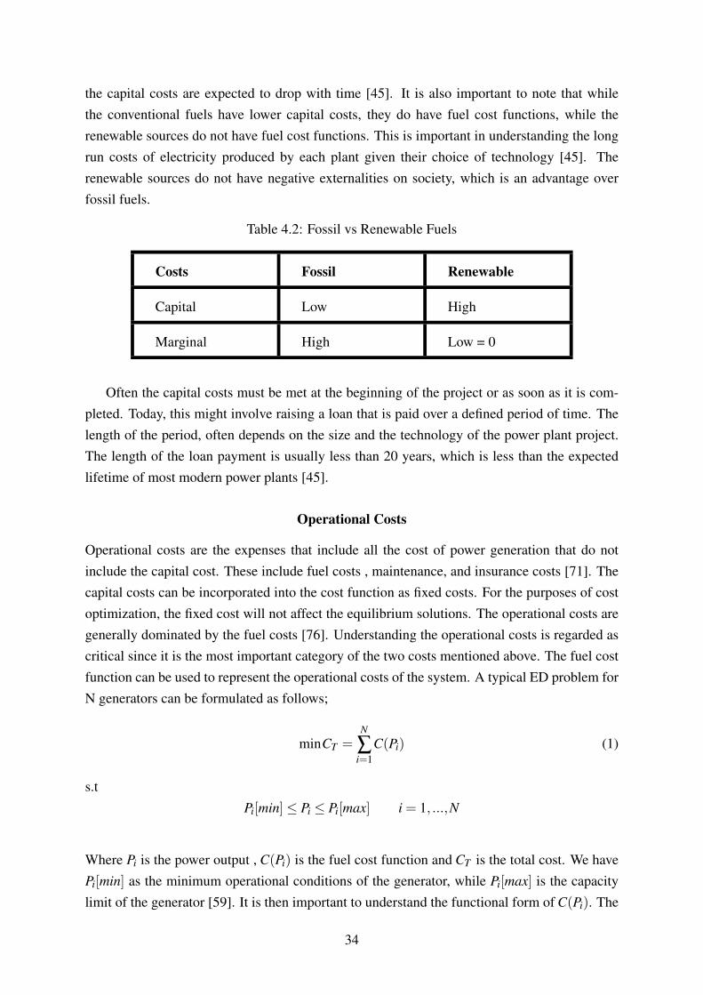
the capital costs are expected to drop with time [45]. It is also important to note that whilethe conventional fuels have lower capital costs, they do have fuel cost functions, while therenewable sources do not have fuel cost functions. This is important in understanding the longrun costs of electricity produced by each plant given their choice of technology [45]. Therenewable sources do not have negative externalities on society, which is an advantage overfossil fuels.

Table 4.2: Fossil vs Renewable Fuels

Costs Fossil Renewable

Capital Low High

Marginal High Low = 0

Often the capital costs must be met at the beginning of the project or as soon as it is com-pleted. Today, this might involve raising a loan that is paid over a defined period of time. Thelength of the period, often depends on the size and the technology of the power plant project.The length of the loan payment is usually less than 20 years, which is less than the expectedlifetime of most modern power plants [45].

Operational Costs

Operational costs are the expenses that include all the cost of power generation that do notinclude the capital cost. These include fuel costs , maintenance, and insurance costs [71]. Thecapital costs can be incorporated into the cost function as fixed costs. For the purposes of costoptimization, the fixed cost will not affect the equilibrium solutions. The operational costs aregenerally dominated by the fuel costs [76]. Understanding the operational costs is regarded ascritical since it is the most important category of the two costs mentioned above. The fuel costfunction can be used to represent the operational costs of the system. A typical ED problem forN generators can be formulated as follows;

minCT =N

∑i=1

C(Pi) (1)

s.tPi[min]≤ Pi ≤ Pi[max] i = 1, ...,N

Where Pi is the power output , C(Pi) is the fuel cost function and CT is the total cost. We havePi[min] as the minimum operational conditions of the generator, while Pi[max] is the capacitylimit of the generator [59]. It is then important to understand the functional form of C(Pi). The

34

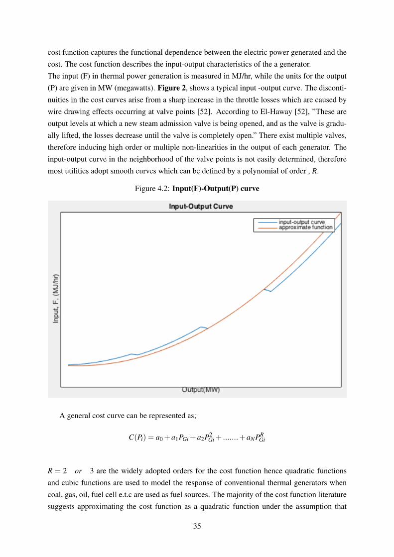
cost function captures the functional dependence between the electric power generated and thecost. The cost function describes the input-output characteristics of the a generator.The input (F) in thermal power generation is measured in MJ/hr, while the units for the output(P) are given in MW (megawatts). Figure 2, shows a typical input -output curve. The disconti-nuities in the cost curves arise from a sharp increase in the throttle losses which are caused bywire drawing effects occurring at valve points [52]. According to El-Haway [52], ”These areoutput levels at which a new steam admission valve is being opened, and as the valve is gradu-ally lifted, the losses decrease until the valve is completely open.” There exist multiple valves,therefore inducing high order or multiple non-linearities in the output of each generator. Theinput-output curve in the neighborhood of the valve points is not easily determined, thereforemost utilities adopt smooth curves which can be defined by a polynomial of order , R.

Figure 4.2: Input(F)-Output(P) curve

A general cost curve can be represented as;

C(Pi) = a0 +a1PGi +a2P2Gi + .......+aNPR

Gi

R = 2 or 3 are the widely adopted orders for the cost function hence quadratic functionsand cubic functions are used to model the response of conventional thermal generators whencoal, gas, oil, fuel cell e.t.c are used as fuel sources. The majority of the cost function literaturesuggests approximating the cost function as a quadratic function under the assumption that

35

the incremental cost curves of the thermal units are monotonically increasing piecewise linearfunctions [76, 52]. Thermal power plants widely use quadratic fuel cost function [76]. Thefollowing is an example of a cost function as used in [76];

Ci(PGi) = a+bPGi + cP2Gi (2)

where PGi = electrical power output , a, b, and c = fuel cost coefficients.The cost of electricity production is quadratic in the electric power output. This models suf-ficiently the increase in costs of production as the power output increases. Most developingcountries use energy from fossil fuels in thermal power plants, therefore this cost function islikely to be applicable in the case of developing countries. When the input-output curve cannotbe approximated by a quadratic function, a function with, R > 2, that captures this non-linearitywould be more appropriate for use in modeling costs of generating electricity in thermal plants.A more complex version of the cost function of thermal power plants is shown in [72], whichoften used when the quadratic function does not accurately model the input -output data. Theyconsider a cubic cost function as follows;

Ci(Pi) = a+bPi + cP2i +dP3

i (3)

Where Pi = electric power output,a, b, c and d = fuel cost coefficients.

Can one accurately estimate the parameters of the cost function for a power plant? Accu-rately estimating the cost function parameters is important in optimizing the objective function(1). If the cost function is not a good representative of the real cost function, this rendersthe optimization of (1) misleading. Artificial intelligence methods like fuzzy logic and neuralnetworks have been used to estimate the cost function parameters. Optimization methods likeparticle swarm optimization and genetic algorithm have also been used to accurately estimatethe fuel cost curves [71, 59, 53, 69].

Electricity Theft

In order to maintain the balance between power generated and power demand, a utility supplierhas to account for the energy lost during transmission and distribution (T&D). This loss ofenergy is incorporated into the cost function of the supplier. For a stable system, this loss ofenergy can be accounted for with high degree of accuracy. If a utility supplier cannot accuratelycalculate these losses, this can lead to undesirable results like black-outs. One reason that canlead to an inaccurate estimation of energy losses is not accounting for theft in the network.Joseph argues that setting the right electricity prices may not suffice in the reduction of financialinstability of the utilities when there is theft in the market [61]. It is important to include allfactors that contribute to energy losses, in order to meet demand in an efficient way.

36

Theft of electricity is defined as the use of electrical power without a contract with a supplierwith total or partial bypassing of the metering system or interfering with the metering systemso as to alter its measurements [70]. Total bypassing (tapping), as shown in Figure 4.3a,usually occurs when a formal consumer supply electricity to their unconnected neighbors. Thetapping happens before the formal consumer’s meter. This energy provided to the informalconsumer is not accounted for in the cost charged to the formal customer. This type of theftis common in developing countries especially in high density suburbs in large cities [70]. Theclose proximity of the houses make it easier to connect two or more houses to one meter. Thisallows the families to split the bill amongst two or more families. This reduces the cost perfamily since the cost per month is split amongst families, this incentive outweighs the costof being caught by the authorities. The families take advantage of the poor fraud detectionmethods in many developing countries. Figure 4.3b, shows an example of current bypass, thisoccurs when current is rerouted from phase input to phase output bypassing the meter in theprocess. Therefore the current supplied to the load cannot be measured and hence the powerusage cannot be measured. The meter will not show accurate measures of power consumed.

Figure 4.3: Illustrations of Electricity Theft

(a) Tapping (b) Current bypass

Electricity theft include billing irregularities and unpaid bills. Levels of electricity theftranged from 0.5 % in the US to as high as 35 % in Bangladesh in 1998 [70]. The standardmethod of measuring electricity theft is using the analysis of the transmissions and distribu-tion(T&D) losses. T&D measures the difference between the amount of electricity generatedinto the grid and the amount that is sold to the consumers. When an accurate calculation of(T&D) is made, theft may contribute significantly to the unaccounted losses [70]. Using thedata from the World Bank’s Development Indicators (2017), we can show the levels of T&Dlosses for individual countries in 1990 and 2014. Figure 4, shows a graphical representationof the losses for a range of countries in 2014. The developing countries incur higher lossescompared to the developed countries. Some places like Togo face as high as 72% losses.

37

Figure 4.4: T& D Losses

While the country comparison is important, the regional comparison of changes in T&Dlosses is also valuable in assessing the regions that are mostly affected by large T&D losses.Figure 5, shows T&D losses of each region in 1990 and 2014.

Figure 4.5: Average T& D Losses by Region

The graph shows that regions like Europe , North America and East Asia have seen a de-cline in T&D losses over time, while regions like Sub Saharan Africa, South East Asia, MiddleEast and Latin America have seen an increase in the average T&D losses. These are also theregions that have the greatest number of least developed countries compared to other regionsthat have seen a decline in T&D losses. The Middle East has seen a number of military conflictsbetween 1990 and 2014 , and this might be a reason for the increase in T&D losses since warcan compromise the infrastructure of the hosting country.

38

In the literature power systems with 16≤%(T &D)≤ 40%, have been viewed as systems withextensive theft, while (T &D)≥ 40, are systems with serious problems [70]. Due to significantimprovements in technology we expect a reduction in (T&D)losses. Therefore the definition ofextensive theft and severe theft as used in [70] is not applicable in today’s conditions. Instead,we can redefine the (T&D) ranges as ; 10≤%(T &D)≤ 20%, are systems with extensive theft,while (T &D)≥ 20, for systems with severe theft problems. We define levels of theft severity as;0,1,2 where 0(normal) =%(T &D)≤ 10 , 1(extensive) = 10≤%(T &D)≤ 20% and 2(severe)

≤ 20. Using the data from the World Bank’s Development Indicators(2017), we obtain Table1 and Table 2 as in [70].

Table 4.3: Country Classification

T/D Loss(%) Number ofCountries

Overall %

0-10 (normal) 59 45.04

10 -20(extensive) 53 40.46

≥ 20 (severe) 19 14.50

Total 131 100

39

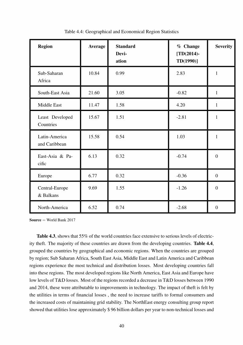
Table 4.4: Geographical and Economical Region Statistics

Region Average StandardDevi-ation

% Change[TD(2014)-TD(1990)]

Severity

Sub-SaharanAfrica

10.84 0.99 2.83 1

South-East Asia 21.60 3.05 -0.82 1

Middle East 11.47 1.58 4.20 1

Least DevelopedCountries

15.67 1.51 -2.81 1

Latin-Americaand Caribbean

15.58 0.54 1.03 1

East-Asia & Pa-cific

6.13 0.32 -0.74 0

Europe 6.77 0.32 -0.36 0

Central-Europe& Balkans

9.69 1.55 -1.26 0

North-America 6.52 0.74 -2.68 0

Source = World Bank 2017

Table 4.3, shows that 55% of the world countries face extensive to serious levels of electric-ity theft. The majority of these countries are drawn from the developing countries. Table 4.4,grouped the countries by geographical and economic regions. When the countries are groupedby region; Sub Saharan Africa, South East Asia, Middle East and Latin America and Caribbeanregions experience the most technical and distribution losses. Most developing countries fallinto these regions. The most developed regions like North America, East Asia and Europe havelow levels of T&D losses. Most of the regions recorded a decrease in T&D losses between 1990and 2014, these were attributable to improvements in technology. The impact of theft is felt bythe utilities in terms of financial losses , the need to increase tariffs to formal consumers andthe increased costs of maintaining grid stability. The NorthEast energy consulting group reportshowed that utilities lose approximately $ 96 billion dollars per year to non-technical losses and

40

electricity theft contributes significantly to these losses [65]. It notes that these losses are crip-pling to both the consumers and the utilities as they result in price hikes to formal customers,financially unsustainable markets and reduce the resources for future capital investments. Evi-dence show that countries with political instability, high levels of corruption, low governmenteffectiveness and low effective accountability face high levels of theft [70]. Most developingcountries if not all, face some or all of the conditions that encourage high levels of theft. Whilethere are proven remedies for theft like tamper-proof meters, regular monitoring and inspection,they still lag behind in implementation of these methods compared to the developed world. Itis important for utilities in these countries to consider the effects of theft for optimal operationsin these countries.

Public Utility Operational Costs

The cost functions (2) and (3) only model the cost incurred from production, and do not modelthe additional cost incurred by the utility due to electricity theft. An appropriate model that in-corporates both the cost due to generation and theft is required for modeling developing coun-tries generation costs. The cost incurred due to theft is especially important to a state ownedutility (incumbent) that maintains the grid. An accurate understanding of the cost structure en-able the utility to make optimal decisions. In order to maintain the grid load the incumbent isforced to produce more electric energy in the presence of theft to maintain grid stability than itwould to meet its formal demand. We define grid stability as the maintenance of a balance be-tween supply and demand of electricity. Grid instability can lead to blackouts. While there areother causes of blackouts like weather, power plant failure e.t.c, our focus is on the blackoutsthat are caused by demand exceeding supply. Blackouts cause both social and economic costs[10]. The dependence of productivity and social welfare on the access of regular and uninter-rupted electricity supply is well established. Both factors contribute to economic development,therefore uninterrupted electricity supply is important for economic growth. A number of stud-ies have estimated the social and economic costs of black out. Different models have beendeveloped to accurately estimate these losses [54, 43]. A government in a developing countrymay seek to minimize these losses by regulating that the incumbent must maintain grid stability.Since the state has social, economic and political reasons to ensure grid stability, therefore theincumbent utility is required by law to guarantee grid stability. The state can argue that the lackin supply is not a result of lack of energy sources but the choice of the incumbent to not meetdemand. This is especially true in developing countries where state owned monopoly oftenpurchase fossil fuels at prices lower than the market value. By making a statutory requirement,the incumbent utility is forced into maintaining grid stability. In addition, it can be the casethat the incumbent utility losses due to blackouts are higher than the costs of maintaining gridstability.

41

Chisari and Kessides considered an incumbent utility that is required to maintain grid stability.This means that any theft that occurs, has to be modeled into the cost function of the utility.Including theft in the cost function model is consistent with the argument in [61] on the impor-tance of including cost due to theft in the optimization problem. They adopted a cost functionfor the incumbent that considers the cost incurred by the incumbent due to theft. Since tappingis more rampant compared to other forms of theft, their model only considers the costs due totapping. They adopt a convex cost function in the size of the network, N. Let, N, be the numberof customers that are formally connected to the network. This implies that as the network sizeincreases, the cost incurred by the utility provider increases since the amount of fuel needed tomeet demand is directly proportional to the network size. They use N as a proxy of the amountof electricity produced. This assumption is valid for an incumbent that maintains grid stability.They consider a market with ,M potential consumers and the incumbent is currently servinga network size N. The remaining M−N consumers either have no access, or a certain ρ ofthem are stealing service from the grid through illegal connections. The following is the costfunction of the incumbent that is convex in N ;

Cρ(N) = F +aN + c[ρM+(1−ρ)N]2, a > 0, c > 0. (4)

Where ρ is the percentage of customers stealing services from the utility,We can show that this cost function (4) has the same functional form as (2) and that it is onlyconvex in the size of the network, N. The following paragraphs explain why equation (4)captures the cost function of an electricity producer in a developing country.We assume that theft only occurs when there is a difference between the market size (M) andthe network size (N), since they only considered theft due to tapping, thus M > N for ρ ∈ [0,1). Let Cρ be the cost function for any ρ ∈ [0,1]. Since Cρ is the cost function for any ρ ∈ (0,1),then we have C1 >Cρ >C0. Therefore, Cρ ∈ [C0,C1], in other words, as ρ increases , the costincurred by the incumbent increases. We can also expand (4) to illustrate how it captures thecost incurred by the incumbent. The following is the expanded version of (4);

Cρ(N) = F +aN +2cρ(1−ρ)MN + c(1−ρ)2N2 + cρ2M2 (5)

If we substitute for the extreme cases of ρ we arrive at C1 and C0 as (9) and (11).However thisformulation does not explain the interaction term MN. In (5), the interpretation is that as M andN increases, the cost incurred by the utility provider increases. However, for a given market, M

is fixed, therefore M is part of the coefficient 2cρ(1−ρ)M of N, which is a variable. In orderto understand this term, re-write (4);

Cρ(N) = F +aN + c[N +ρ(M−N)]2 (6)

42

We can then expand (6) to get the following;

Cρ(N) = F +aN + c[N2 +2ρ(M−N)N +ρ2(M−N)2] (7)

The cost function is convex in both N and M−N as shown by equation (7). It should be notedthat at any given point in time , M is fixed. The cost function increases as [M−N] shrinks,however the rate of increase is less than the rate of increase of the cost function when ρ = 0.

Lemma 2 The rate of increase of the cost function when ρ ∈ (0,1) is less than the rate of

increase of the cost function when ρ = 0 i.e dCρ

dN < dC0

dN .

Proof. We show this by proving that d2Cρ

dN2 < d2C0

dN2 , since each second order derivative measuresthe rate of change of the first derivatives i.e dCρ

dN and dC0

dN . We can take the second derivatives ofCρ w.r.t N for ρ = 0 and ρ ∈ (0,1);

d2C0

dN2 = 2c

andd2Cρ

dN2 = 2c(1−ρ)

Since ρ ∈ (0,1), we have d2Cρ

dN2 < d2C0

dN2 which implies that dCρ

dN < dC0

dN Intuitively, Cρ alreadyaccounts for the costs incurred for supplying some of the informal network, therefore if Nincreases, the incumbent already accounted for the cost of part of the change in N. This is notthe case when ρ = 0. For completeness, we note that dCρ

dN = 0 when ρ = 1. Thus , dC0

dN > dCρ

dN >dC1

dN .

Lemma 3 (4) is only convex in N iff M is a constant i.e it has the same functional form as (2)

Proof. Re-arrange(7) as follows;

C(N) = [F + cρ2M2]+ [a+2cρ(1−ρ)M]N + c(1−ρ)2N2

Let F = [F + cρ2M2], a = [a+2cρ(1−ρ)M] and c = c(1−ρ)2, therefore;

C(N) = F+aN + cN2 (8)

This is consistent with the fuel cost function (2) which is convex in the amount of electricitypower produced. It also increases as ρ increases, as explained above.

Lets take the extreme conditions where ρ = 1 and ρ = 0. When ρ = 1, there exist perfectstealing and the whole population ,M , has access to the utility services. Thus;

C1(N) = F +aN + cM2 (9)

43

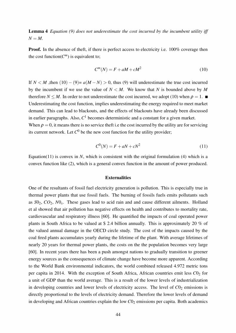
Lemma 4 Equation (9) does not underestimate the cost incurred by the incumbent utility iff

N = M.

Proof. In the absence of theft, if there is perfect access to electricity i.e. 100% coverage thenthe cost function(Cm) is equivalent to;

Cm(N) = F +aM+ cM2 (10)

If N < M ,then (10)− (9)= a(M−N) > 0, thus (9) will underestimate the true cost incurredby the incumbent if we use the value of N < M. We know that N is bounded above by M

therefore N ≤M. In order to not underestimate the cost incurred, we adopt (10) when ρ = 1.Underestimating the cost function, implies underestimating the energy required to meet marketdemand. This can lead to blackouts, and the effects of blackouts have already been discussedin earlier paragraphs. Also, C1 becomes deterministic and a constant for a given market.When ρ = 0, it means there is no service theft i.e the cost incurred by the utility are for servicingits current network. Let C0 be the new cost function for the utility provider;

C0(N) = F +aN + cN2 (11)

Equation(11) is convex in N, which is consistent with the original formulation (4) which is aconvex function like (2), which is a general convex function in the amount of power produced.

Externalities

One of the resultants of fossil fuel electricity generation is pollution. This is especially true inthermal power plants that use fossil fuels. The burning of fossils fuels emits pollutants suchas S02, CO2, N0x. These gases lead to acid rain and and cause different ailments. Hollandet al showed that air pollution has negative effects on health and contributes to mortality rate,cardiovascular and respiratory illness [60]. He quantified the impacts of coal operated powerplants in South Africa to be valued at $ 2.4 billion annually. This is approximately 20 % ofthe valued annual damage in the OECD circle study. The cost of the impacts caused by thecoal fired plants accumulates yearly during the lifetime of the plant. With average lifetimes ofnearly 20 years for thermal power plants, the costs on the the population becomes very large[60]. In recent years there has been a push amongst nations to gradually transition to greenerenergy sources as the consequences of climate change have become more apparent. Accordingto the World Bank environmental indicators, the world combined released 4.972 metric tonsper capita in 2014. With the exception of South Africa, African countries emit less C02 fora unit of GDP than the world average. This is a result of the lower levels of industrializationin developing countries and lower levels of electricity access. The level of C02 emissions isdirectly proportional to the levels of electricity demand. Therefore the lower levels of demandin developing and African countries explain the low C02 emissions per capita. Both academics

44

and policy makers are concerned about the best way to reduce greenhouse effects and minimizethe economic effects that can arise from such action.

Tradable Permits vs Emission Taxes

On December 10, 1997, 160 countries signed the Kyoto Protocol agreement on limiting emis-sions of greenhouse gases. This set in motion the debate on how to efficiently achieve thereduction in pollution in different economies. Economic literature draws a clear distinction be-tween command and control approaches (CAC) and market-based incentives (MBI), with thelatter being preferred over the former [125]. Two MBI instruments have been used as a con-trol strategy for green house emission reduction: Enviromental taxes and tradable permits havebeen adopted by different countries over the past two decades. The main challenge to policymakers is knowing which instrument to adopt and under what conditions it will be most effi-cient. There is established economic literature that details the efficient conditions to implementeither the environmental tax or the tradable permits.

Environmental Taxes

Environmental taxes are known as Pigouvian taxes. This is a tax that is charged on any marketactivity that impose costs on the society (negative externalities). The intent of this tax is tomove the market from an inefficient point to an efficient point where the cost to society is lowerthan the inefficient point. In energy economics, this can be achieved by levying a carbon tax onpower suppliers. The tax levied on the suppliers needs to be equal to the total damage causedby the extra unit of emissions. This means that the tax needs to be a true reflection of the cost tosociety, therefore the power supplier has an incentive to reduce emissions until a unit reductionin emission is equal to the social damage [60]. According to Van Heerden, the Pigouvian taxhas four effects on an economy [58];

1. They result in an increase in production costs in energy intensive industries. Thus, re-ducing export demands of energy intensive goods , making imports a more attractivealternative. This reduces the output in energy intensive trade related sectors. There isalso a shift in labor supply from energy intensive sectors to less energy intensive sectors.

2. They increase revenue collected by the government; however, this revenue needs to bedistributed in order to avoid a reduction in purchasing power. Thus resulting in a decreasehousehold consumption.

3. They cause a decrease in GDP because the tax causes an increase in prices thereby in-creasing inflation. The unskilled worker wage rate is proportional to the CPI increases asinflation rises thereby reducing unskilled labor in the workforce.

45

4. They cause substitution form energy and energy rich commodities to sectors with lowenergy consumptions. This reduces demand in energy, therefore resulting in a decreasein greenhouse gas emissions.

Tradable permits

Tradable permit system requires the regulator to investigate and set a cap on the levels of pollu-tion allowed for a specific industry. In this case it is the levels of pollution allowed for electricitygeneration. Once the pollution cap is established, the regulator issues permits that amounts tothe cap limit e.g. a cap of 3 000 000 tonnes of C02 will require 3 000 000 permits. These per-mits are either distributed to the participating firms or a sold in a blind auction (highest bidderwins). No firm is allowed to emit pollution without acquiring the equivalent number of permits.After acquiring the permits, a firm can buy or sell permits to/from other firms. Tradable per-mits can induce innovation and development as firms seek ways to minimize costs. A potentialshortfall of tradable permits is in dealing with market power. Koustaal and Xepapadeas sepa-rately established that firms when firms behave as price setters , the gains of tradable permitsare lost [62, 75]. The following table summarizes the main finding of the discussion in [125];

Table 4.5: Summary of Efficiency Considerations and Market Structure

Market Struc-ture

Emission Tax Tradable Per-mits

Perfect Competi-tion

Efficient Efficient

Noncompetitivemarket in theoutput market

Efficient can beachieved by suit-ably adjusting thePigouvian tax butonly if firms areall identical

Inefficient but lit-erature suggeststhat efficiencylosses may besmaller thanunder an emis-sion tax(whenfirms have dif-ferent pollutiontechnologies).

Noncompetitivemarket structurein the permitsmarket

N.A Inefficient

Source = Norregaard and Repellin-Hill 2000

The importance of privatization is supported by the inefficient levels that are achieved byboth the emissions tax and tradable permits in a monopolistic market [47]. By introducing

46

competition, the market becomes efficient under both the emission tax or the tradable permits.It is important to note that the environmental tax achieves social optimum [68] when the firmscausing pollution are identical i.e they use similar technology for electricity production. In thecase of dissimilar technologies, only the firm specific environmental tax achieves the socialoptimum [68]. We model the emission tax as part of the cost to the utility. Therefore we extendthe cost function by Chisari and Kessides to include the cost of emission tax. We assume thatthe marginal cost of emission increase as the production capacity increases. Let, νi be theemission tax imposed on the utility. Therefore the new cost function is;

Cρ(N) = F +aN + c[ρM+(1−ρ)N]2 +νN2, a > 0, c > 0 ν > 0. (12)

Entrant Firm Operational Costs

For the case of the entrant firm; the entrant does not own the grid network, but it can directlybill its own consumers. Unlike the incumbent that considers theft as a cost. The entrant doesnot carry the burden of maintaining grid stability i.e it only incurs costs of supplying electricityto its own network. Therefore it does not consider costs due to theft. This is a clear distinctionbetween the incumbent and the entrant utility. The cost function for the entrant is equivalent tothe cost function of the incumbent supplier when ρ = 0. Any theft that occurs for the entrantwill be considered as revenue that is not realized. This will be true in the presence of currentbypass theft as illustrated in Figure 3b. If the entrant firm does not directly collect revenuefrom the customers, it can receive its revenue from a third part namely a local municipal or thegovernment. This can lead to to the entrant not receiving all the revenue it should be receivingfrom its consumers. Let, a fraction τ of the revenue owed to the supplier by the governmentis not paid to the utility. This is called unrealizable revenue. This is common in markets withpoor government systems. We also include the adjustment costs as part of the cost function. Anentrant utility that adopts the conventional fuels for energy production uses the quadratic costfunction to model the costs incurred for its optimization problem. The entrant firm also facesan environmental tax ν for greenhouse emissions. We define the cost function of the entrantfirm as follows;

C(Ne) = F +aNe + cN2e +φ Ne

2+νeN2

e , ae > 0, ce > 0 νe > 0. (13)

Where, F ≥ 0 are the fixed costs for each utility provider, φ N2 is the adjustment cost in networksize, ν is the emissions tax.The cost function of the entrant (12) is equivalent to (11), for the incumbent, when ρ = 0.

If τ > 0, we represent the unrealized revenue in the profit function of the entrant. Therefore,the general profit function of the entrant utility using the cost function described above is as

47

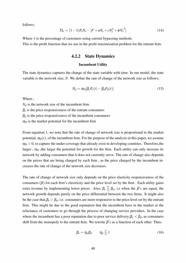
follows;Πe = (1− τ)PeNe− [F +aNe + cN2

e +φ Ne2] (14)

Where τ is the percentage of customers using current bypassing methods.This is the profit function that we use in the profit maximization problem for the entrant firm.

4.2.2 State Dynamics

Incumbent Utility

The state dynamics captures the change of the state variable with time. In our model, the statevariable is the network size, N. We define the rate of change of the network size as follows;

Nd = αD[βePe(t)−βdPd(t)] (15)

Where ,Nd is the network size of the incumbent firm.βe is the price responsiveness of the entrant consumersβd is the price responsiveness of the incumbent consumersαD is the market potential for the incumbent firm

From equation 1, we note that the rate of change of network size is proportional to the marketpotential, αD(t), of the incumbent firm. For the purpose of the analysis in this paper, we assumeαD > 0, to capture the under-coverage that already exist in developing countries. Therefore,thelarger , αD ,the larger the potential for growth for the firm. Each utility can only increase itsnetwork by adding consumers that it does not currently serve. The rate of change also dependson the prices that are being charged by each firm , as the price charged by the incumbent in-creases the rate of change of the network size decreases.

The rate of change of network size only depends on the price elasticity responsiveness of theconsumers (β ) for each firm’s electricity and the price level set by the firm . Each utility gainsextra revenue by implementing lower prices. Also, βe T βd , i.e when the β ′s are equal, thenetwork growth depends purely on the price differential between the two firms. It might alsobe the case that,βe > βd , i.e. consumers are more responsive to the price level set by the entrantfirm. This might be due to the good reputation that the incumbent have in the market or thereluctance of customers to go through the process of changing service providers. In the casewhere the incumbent has a poor reputation due to poor service delivery;βe < βd , as consumersshift from the monopoly to the entrant firm. We rewrite β ′s as a function of each other. Thus;

βe = ηdβd ηd T 1 (16)

48

Therefore equation(15) can be written as ;

Nd = βdαD[ηdPe−Pd] (17)

From (15), Nd > 0 when ηdPe > Pd which means PePd

> 1ηd

. This is a necessary and sufficientcondition. We analyze three possible condition, (a)βe = βd (b) βe > βd and (c) βe < βd . Theproofs of these scenarios are shown in the appendix.

Entrant Utility

By following the same analysis as above, we can formulate the state dynamic equation of theentrant firm as follows;

Ne = αE [βdPd−βePe] (18)

Where ,αE is the market potential for the entrant firmNe is the network size of the entrant firm.βe is the responsiveness of the consumers to the entrant priceβd is the responsiveness of the consumers to the incumbent price

From equation(2), the rate of change of the network size of the entrant is proportional to themarket potential M−Ne > 0. When the β ′s are equal, the network growth depends on the pricedifferential between the two firms. From (2), Ne > 0 when βdPd > βePe which means Pd

Pe> βe

βd

. We have, Pd > Pe, when βe = βd , intuitively customers would prefer joining a network wherethe prices are lower. We rewrite β ′s as a function of each other. Thus;

βd = ηeβe ηe T 1 (19)

Therefore equation(1) can be written as;

Ne = βeαE [ηePd−Pe] (20)

From (5), Ne > 0 when ηePd > Pe which means PdPe

> 1ηe

. This is a necessary and sufficientcondition. We analyze three possible condition, (a)βe = βd (b) βe > βd and (c) βe < βd . Theproofs of these conditions are similar to the ones shown for the incumbent.

49

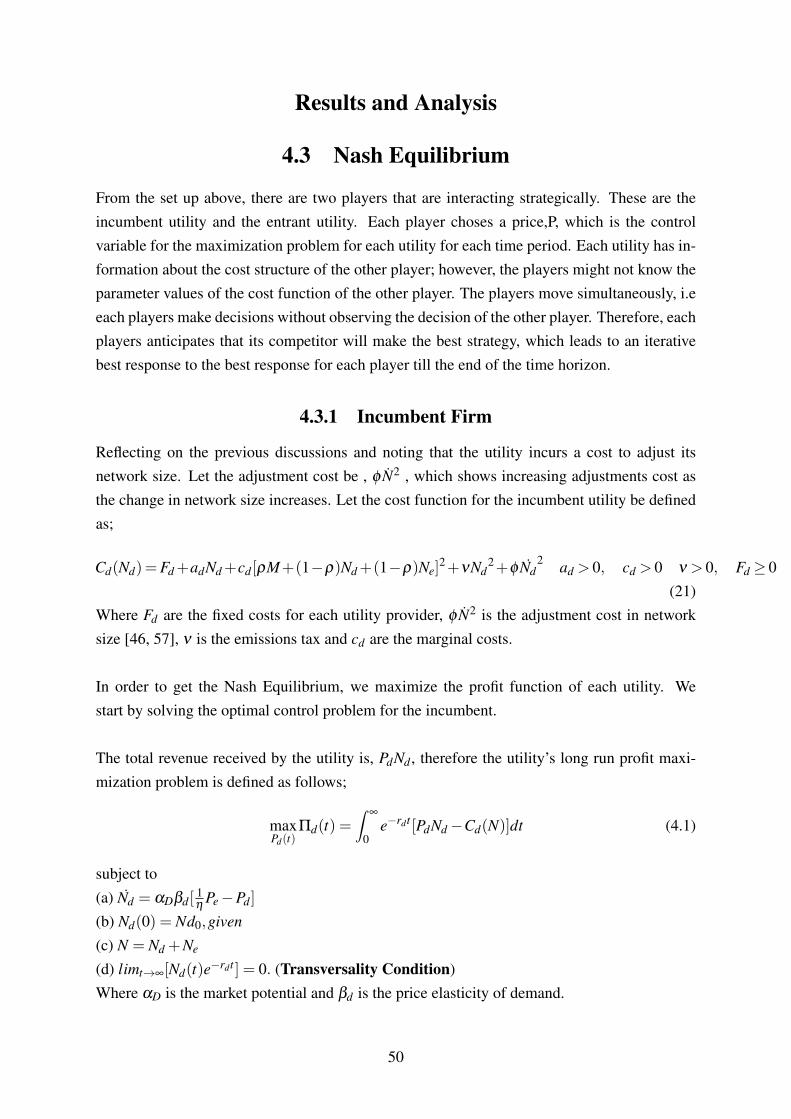
Results and Analysis

4.3 Nash Equilibrium

From the set up above, there are two players that are interacting strategically. These are theincumbent utility and the entrant utility. Each player choses a price,P, which is the controlvariable for the maximization problem for each utility for each time period. Each utility has in-formation about the cost structure of the other player; however, the players might not know theparameter values of the cost function of the other player. The players move simultaneously, i.eeach players make decisions without observing the decision of the other player. Therefore, eachplayers anticipates that its competitor will make the best strategy, which leads to an iterativebest response to the best response for each player till the end of the time horizon.

4.3.1 Incumbent Firm

Reflecting on the previous discussions and noting that the utility incurs a cost to adjust itsnetwork size. Let the adjustment cost be , φ N2 , which shows increasing adjustments cost asthe change in network size increases. Let the cost function for the incumbent utility be definedas;

Cd(Nd)=Fd+adNd+cd[ρM+(1−ρ)Nd+(1−ρ)Ne]2+νNd

2+φ Nd2 ad > 0, cd > 0 ν > 0, Fd ≥ 0

(21)Where Fd are the fixed costs for each utility provider, φ N2 is the adjustment cost in networksize [46, 57], ν is the emissions tax and cd are the marginal costs.

In order to get the Nash Equilibrium, we maximize the profit function of each utility. Westart by solving the optimal control problem for the incumbent.

The total revenue received by the utility is, PdNd , therefore the utility’s long run profit maxi-mization problem is defined as follows;

maxPd(t)

Πd(t) =∫

∞

0e−rdt [PdNd−Cd(N)]dt (4.1)

subject to(a) Nd = αDβd[

1η

Pe−Pd]

(b) Nd(0) = Nd0,given

(c) N = Nd +Ne

(d) limt→∞[Nd(t)e−rdt ] = 0. (Transversality Condition)Where αD is the market potential and βd is the price elasticity of demand.

50

The constraint (a) represent the change in the network size due to the price differential, (b)represents the initial network size of the the utility while (c) is the number of consumers servedby both utility firms.

Transversality Conditions

The problem defined in this paper is an infinite horizon optimization problem. Since this is adiscounted problem, it is easy to see that as, t→∞, the objective function Πd(Pd(t),Nd(t),T )→0. We know that the state variable Nd(t) is bounded by M, the size of the market. We use theresults on transversality obtained by Chiang [48]. The first order conditions of maximizing theobjective function with a small perturbation is defined as follows;

∂Πd

∂ε= e−rdt [

∫∞

0[(

∂H∂Nd

+ λd)q(t)+∂H∂Pd

p(t)]dt + limt→∞

[H]t=T ∆T − limt→∞

λd(t)∆NT ] = 0 (23)

Where Nd is the state variable,Pd is the control, H is the Hamiltonian, p(t) and q(t) are theperturbing curves for P and N. In order to satisfy the first order condition all the three distinctterms above have to equal zero. Let; A =

∫∞

0 [( ∂H∂Nd

+ λd)q(t)+ ∂H∂Pd

p(t)]dt

B = limt→∞

[H]t=T ∆T

C = limt→∞

λ (t)∆NT

Only B and C give rise to transversality conditions.Since time is not fixed, we know that ∆T > 0. Therefore, one transversality condition thatmakes B = 0 is ;

limt→∞

[H]t=T = 0

It is known that Nd(t) is bounded by M. This implies that ∆NT = 0. This condition is sufficientto make C = 0 without imposing any restrictions on λd(T ) . We have lim

t→∞NT = N∞. For the

discounted optimization problem, we have ;limt→∞

Nde−rdt = e−rdtN∞

We can rewrite this condition as follows;

limt→∞

Nde−rdt = 0

This is the transversality condition we will use in this paper. The same conditions hold for theentrant firm.

Let the Hamiltonian be defined as;

Hd(Nd,Pd,T,λd) = e−ritΠ(Pd,N)+λdNd

51

Where λd = costate variable or the shadow price.

Hd(Nd,Pd,T,λd) = e−rit [PdNd−Cd(Nd)]+λdαDβd[1η

Pe−Pd]

From the Hamiltonian we have the following first order conditions necessary for intertemporalmaximization problem [67];

∂Hd

∂Pd= HdPd = e−rdt(Nd +2φβ

2d α

2D[

1η

Pe−Pd])−λdαDβd = 0 (24)

∂Hd

∂Nd= HdNd = e−rdt(Pd−Cd(Nd)) =−λ

′d (25)

Lemma 5 The first-order conditions (24) and (25) are sufficient for optimum conditions iff

2φβ 2d α2

DC(Ni)−1 > 0.

Proof. The Mangasarian Sufficiency Theorem [63], states that the necessary conditions of theMaximum Principle are also sufficient for the global maximization of the objective function ifthe Hessian matrix of Hi, denoted by Hi, is negative definite, i.e.

Hd =

HNdNd HNdPd

HPdNd HPdPd

< 0

From (3) and (4) we have the following ;

HNdNd =−e−rdtC(Nd)

HNdPd = HPdNd = e−rdt

HPdPd =−2φβ2d α

2De−rdt

Therefore,HNdNd HPdPd −H2

PdNd= e−2rdt [2φβ

2d α

2DC(Nd)−1]. (26)

Since C(Nd)> 0 by construction then HNdNd < 0, if 2φβ 2d α2

DC(Nd)−1 > 0 then Hd is negativedefinite. That means the Hamiltonian Hd is concave in (Nd,Pd) and the Mangasarian Suffi-

ciency Conditions are met. Similar to [81], we define the current value Hamiltonian and it ismaximized with respect to Pd . The following is the Hamiltonian equation;

Hc = Π(Pd,Nd)+λcβdαD[1η

Pe−Pd]

52

where λc is the current value Langrage multiplier.

Lemma 6 The first order condition of Hc at the optimum is given by;

∂Π(Pd,Nd)

∂Pd− βd

rd

∂Π

∂Nd= 0 (27 a)

Proof. First define λc as;λc = λerdt (27 b)

Rearanging (b) we have ;λ = λce−rdt

Take the derivative with respect to t ;

erdtλ′ = λ

′c− rdλc (c)

From the definitionHc = ertH

Thus;HNd

c = erdt(HNd) =−erdtλ′c

From Hc;

HNdc =

∂Π

∂Nd= rdλc−λ

′c

make λc the subject ;

λc = [λ ′c +∂Π(P,N)

∂Nd]

1rd

we also have;

HPc =

∂Π

∂Pd−λcβdαD = 0 (27 c)

sub λc into HPc to get,

∂Π(P,N)

∂Pd− [λ ′c +

∂Π(P,N)

∂Nd]βdαD

rd= 0

∂Π(P,N)

∂Pd− λ ′cβd

rd− ∂Π(P,N)

∂Nd

βdαD

rd= 0

At the optimum, λc is a constant, therefore, λ ′c = 0, thus;

∂Π(P,N)

∂Pd=

∂Π(P,N)

∂Nd

βdαD

rd

From (27a), the first term , ∂Π(P,N)∂Pd

, measures the marginal increase in the current profit for

the incumbent firm due to an increase in the price it set. While the second term, ∂Π(P,N)∂Nd

βdαDrd

,

53

measures the marginal decrease in future profits due to the change in the decrease in the networksize of the utility induced by the increase in price. The change in network size is proportionalto βdαD

rd. An increase in Pd , changes the price ratio Pd

Pe, or in other words, it reduces the price

differential between the incumbent and the entrant firm. This can lead to a loss of consumers tothe entrant firm and reduces the expansion rate of the firm. From (27a), the loss of consumersdepends on the price elasticity of demand, βd . It also depends on the level of future profitdiscount level , rd . If the firm discounts heavily future profits, then the firm will not considerthe increased loss of customers in the long run, but instead it will focus on the increased shortrun profits. The incumbent firm increases its price if ∂Π(P,N)

∂Pd> ∂Π(P,N)

∂Nd

βdαDrd

. Therefore, thefirm will choose an optimal pricing path ,Pd(t), that balances the effects on short run profitsand future profits.

Optimal Size and Pricing Path

From the first order conditions, the following second order differential equation is obtained;

Nd−rdNd−rd +2cdβdαD(1−ρ)2 +2βdαDν

2φβdαDNd =−βdαD

1η

Pe−ad−2cρ(1−ρ)M−2c(1−ρ)2Ne

2φβdαD

(29)

This is a non-homogeneous second order differential equation, it will be solved in two steps.From (29) let;

k =rd +2cdβdαD(1−ρ)2 +2βdαDν

2φβdαD

d =−βdαD

1η

Pe−ad−2cdρ(1−ρ)M−2c(1−ρ)2Ne

2φβdαD

The second order differential equation can be re-written as;

Nd− rdNd− kNd = d

The solution of this differential equation is given by;

Nd(t) = (Nd0−N∗d )e−rd(

ζd−12 )t +N∗d (30)

54

where ζd = [1+2 (rd+2cdβdαD(1−ρ)2+2βdαDν)

(φβdαDr2d)

]12 with ζd > 11 and ,

N∗d = βdαD

1η

Pe−ad−2cdρ(1−ρ)M−2cd(1−ρ)2Ne

rd +2cdβdαD(1−ρ)2 +2βdαDν(31)

From (15a) and (29) the optimal pricing path is given by;

Pd(t) =1η

Pe +rd

βdαD

ζd−12

(Nd0−N∗d )e−rd(

ζd−12 )t (32)

Where the steady state price ,P∗d is given by;⇒

P∗d =P∗eη

4.3.2 Entrant Profit Maximization

Let the cost function for the incumbent utility be defined as;

Ce(Ne) = Fe +aeNe + ceN2e +νN2

e +φ Ne2 ae > 0, ce > 0 ν > 0, Fe ≥ 0 (33)

The entrant utility’s long run profit maximization problem is defined as follows;

maxPe(t)

Πe(t) =∫

∞

0e−ret [(1− τ)PeNe−Ce(N)]dt (34)

subject to(a) Ne = βdαE [Pd(t)− 1

ηPe(t)],

(b) Ne(0) = Ne0

(c) N(t) = Nd(t)+Ne(t)

(d) limt→∞[Ne(t)e−ret ] = 0.

The Hamiltonian for this problem is given by :

H(Ne,Pe,T,λe) = e−retΠe(Pe,Ne)+βdαE [Pd(t)−

1η

Pe(t)] (35)

Where,Πe(Pe,Ne) = (1−τ)PeNe−Ce(Ne) and λe(t) , is the Lagrange multiplier associated with 35(a).Here the Lagrange multiplier is interpreted as the shadow price , which is the value to the utilityfor an extra customer at time,t.From equation(11) we have the following first order conditions necessary for intertemporal

1Since all the parameters are positive , thus (rd + 2cdβdαD(1−ρ)2 + 2βdαDν) > 0 . The denominator has

positive parameters, therefore (φβdαDr2d > 0 . Thus 2 (rd+2cdβdαD(1−ρ)2+2βdαDν)

(φβdαDr2d

> 0 and ζd > 1

55

maximization problem;

∂H∂Pe

= HPe = e−ret((1− τ)Ne +2φβ2d α

2E [Pd(t)−

1η

Pe])−λeβeαE = 0 (36)

∂H∂Ne

= HNe = e−ret((1− τ)Pe−Ce(Ne)) =−λe (37)

We define the current Hamiltonian as in the case of the incumbent firm. By the same derivation,the following results stands;

Lemma 7 The first order condition of Hc at the optimum is given by;

∂Π(Pe,Ne)

∂Pe=

βdαE

ηre

∂Π(Pe,Ne)

∂Ne(38 a)

Proof. As shown in Lemma 1.2

Optimal Size and Pricing Path

Differentiating (36) with respect to, t,and substituting for λe and λe in (37)to derive the second-order differential equation in Ne.

Ne − reNe −ηre(1− τ)+2ceβdαE +2βdαEν

2φβdαENe = −βdαE

η(1− τ)Pd−ae

2φβdαE(39)

This is a non-homogenous second order differential equation, we solve this in two steps. From(39) let;

k =ηre(1− τ)+2ceβdαE +2βdαEν

2φβdαE

d =−βdαEη(1− τ)Pd−ae

2φβdαE

The solution of this differential equation is given by;

Ne(t) = (Ne0−N∗e )e−re(

ζe−12 )t +N∗e (40)

where ζe = [1+2 (ηre(1−τ)+2ceβdαE+2βdαE ν)(φβdαE r2

e )]

12 with ζe > 12

N∗e = βdαEη(1− τ)Pd−ae

ηre(1− τ)+2ceβdαE +2βdαEν(41)

2proof similar to 1

56

From (34a) and (40) the optimal pricing path is given by;

Pe(t) = η(1− τ)Pd(t)+ηre

βdαE

ζe−12

(Ne0−N∗e )e−re(

ζe−12 )t (42)

Where the steady state price , P∗e is given by;⇒

P∗e = η(1− τ)Pd

4.4 Case Analysis

The optimal pricing path for both the incumbent and the entrant firm show the strategic in-teraction between the two firms over time. Specifically, each firm responds to the price setby its competitor. This is in contrast with the pricing path followed by the monopoly in the[81]. It is this strategic interaction between the two firms that can lead to perfect competi-tion under specific parameter conditions. The role of the policy maker can be one that shiftsthe equilibrium to a perfectly competitive equilibrium. The relative network size scenariosanalyzed in this paper creates 9 possible pricing path, Se,Sd, Se,Cd, Se,Gd, Ce,Sd,Ce,Cd,Ce,Gd,Ge,Sd,Ge,Cd, and Ge,Gd . Under the assumption that the entrantfirm has an initial network size of , Ne0 = 0, then we can eliminate the following cases from ouranalysis; Ge,Sd , Se,Sd, Ce,Gd and Ce,Cd . Under this assumption, competition onlyexists if the entrant firm can grow its network size. This reduces the cases to be analyzed to thefollowing; Ge,Sd,Ge,Cd, and Ge,Gd. The case of , Ge,Sd , can be achieved by bothan increase in prices by both firms or in this case only the entrant is choosing prices that arelower than that of the incumbent form. The case of , Ge,Gd, is one in which both firms areraising their prices. evolution of the pricing path in this case is analyzed in the following para-graphs. The case of, Ge,Cd, can be achieved when both firms follow an increasing pricingpath. The following table summarizes the case analysis in terms of the pricing path;

Table 4.6: Pricing Path

Gd Cd Sd

Ge ↑ P Pd = Peη

?

Se N/A N/A ↓P

One can note that in the case Ge,Cd , we have (Nd0−N∗d ) = 0 therefore Pd(t) = 1η

Pe(t),in this case the incumbent firm initial prices are only adjusted for the price responsiveness ofthe customers between the entrant firm and the incumbent firm. In the case, Ge,Sd ,we have(Nd0−N∗d )> 0 therefore Pd(t) = 1

ηPe+

rdβdαD

ζd−12 (Nd0−N∗d )e

−rd(ζd−1

2 )t > Pe(t), in this case the

57

incumbent firm always has prices higher than that of the entrant firm. These two cases thoughfeasible , they are of less interest in terms of the analysis in this paper. The rest of the analysisfocuses on the case Ge,Gd.

4.4.1 Comparative Statics Analysis

This section focuses on the sensitivity of the objective function values, control variables andstate variables with respect to the parameters in the model. The partial derivatives used in allthe analysis in this section were verified using MATLAB3 function diff and the sign of thepartial derivatives using the isAlways function.

Steady State Network Sizes

Incumbent Firm

The steady state network size of the incumbent firm is given by;

N∗d = βdαD

1η

Pe−ad−2cdρ(1−ρ)M−2c(1−ρ)2Ne

rd +2cdβdαD(1−ρ)2 +2βdαDν(31)

By taking the first order conditions of N∗d with respect to the model parameter, we describehow the steady state network size changes as these parameters change. Since N∗d > 0, letA = 1

ηPe−ad−2cdρ(1−ρ)M−2c(1−ρ)2Ne > 0. The following table summarizes the range

of each parameter under consideration;

3The MATLAB code can be provided upon request

58

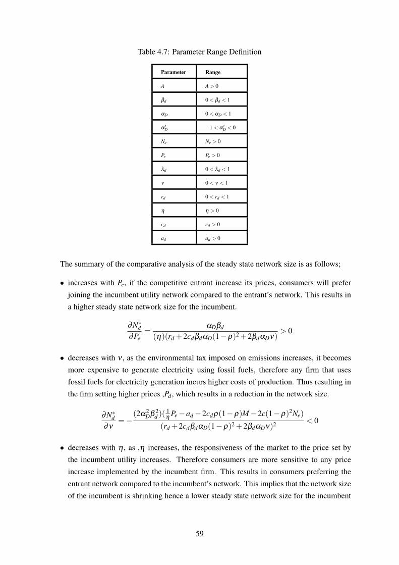
Table 4.7: Parameter Range Definition

Parameter Range

A A > 0

βd 0 < βd < 1

αD 0 < αD < 1

α ′D −1 < α ′D < 0

Ne Ne > 0

Pe Pe > 0

λd 0 < λd < 1

ν 0 < ν < 1

rd 0 < rd < 1

η η > 0

cd cd > 0

ad ad > 0

The summary of the comparative analysis of the steady state network size is as follows;

• increases with Pe, if the competitive entrant increase its prices, consumers will preferjoining the incumbent utility network compared to the entrant’s network. This results ina higher steady state network size for the incumbent.

∂N∗d∂Pe

=αDβd

(η)(rd +2cdβdαD(1−ρ)2 +2βdαDν)> 0

• decreases with ν , as the environmental tax imposed on emissions increases, it becomesmore expensive to generate electricity using fossil fuels, therefore any firm that usesfossil fuels for electricity generation incurs higher costs of production. Thus resulting inthe firm setting higher prices ,Pd , which results in a reduction in the network size.

∂N∗d∂ν

=−(2α2

Dβ 2d )(

1η

Pe−ad−2cdρ(1−ρ)M−2c(1−ρ)2Ne)

(rd +2cdβdαD(1−ρ)2 +2βdαDν)2 < 0

• decreases with η , as ,η increases, the responsiveness of the market to the price set bythe incumbent utility increases. Therefore consumers are more sensitive to any priceincrease implemented by the incumbent firm. This results in consumers preferring theentrant network compared to the incumbent’s network. This implies that the network sizeof the incumbent is shrinking hence a lower steady state network size for the incumbent

59

firm.∂N∗d∂η

=− PeαDβd

(η2)(rd +2cdβdαD(1−ρ)2 +2βdαDν)< 0

• decreases with Ne, since there is strategic interaction between the two firms, an increase inthe entrant firms network size, Ne , this results in the loss of consumers by the incumbentfirm. In other words, the consumers prefer the entrant utility to the incumbent utility.

∂N∗d∂Ne

=− 2αDβd(1−ρ)2

rd +2cdβdαD(1−ρ)2 +2βdαDν< 0

• increases with αD, intuitively as the market potential increases the number of availableconsumers to the incumbent firm is increasing. The firm can increase its steady statenetwork size in a a market with higher potential , therefore the resultant steady statenetwork size is higher.

∂N∗d∂αD

=βd(

1η

Pe−ad−2cdρ(1−ρ)M−2c(1−ρ)2Ne)

rd +2cdβdαD(1−ρ)2 +2βdαDν

−αDβd(2βdν +2βdcd(1−ρ)2)( 1

ηPe−ad−2cdρ(1−ρ)M−2c(1−ρ)2Ne)

(rd +2cdβdαD(1−ρ)2 +2βdαDν)2 > 0

• decreases with rd , as the incumbent firm discounts heavily future profits, it adopts highshort run prices to achieve higher short term profits. This firm sacrifices long run profitsto obtain higher short run profits, as a consequence, the incumbent firm will have a lowersteady state network size.

∂N∗d∂ rd

= −αDβd(

1η

Pe−ad−2cdρ(1−ρ)M−2c(1−ρ)2Ne)

(rd +2cdβdαD(1−ρ)2 +2βdαDν)2 < 0

Entrant Firm

The steady state network size of the entrant firm is given by;

N∗e = βdαEη(1− τ)Pd−ae

η(1− τ)re +2ceβdαE +2βdαEν(41)

Using the same assumptions as in the case of the incumbent firm, the following partial deriva-tives with respect to the parameters are as follows; ∂N∗e

∂Pd> 0 ,∂N∗e

∂ν< 0 , ∂N∗e

∂τ< 0 , ∂N∗e

∂αE> 0

and ∂N∗e∂ re

< 0 The analysis of these partial derivatives is similar to the analysis given for theincumbent firm.

60

Initial Prices

Incumbent Firm

The initial price for the incumbent firm is given by;

Pd(0) =1η

Pe(0)+rd

βdαD

ζd−12

(Nd0−N∗d ) (43)

Since (Nd0−N∗d ) < 0 the prices set by the incumbent firm is lower than 1η

Pe(0) . Each firm’s initial price also depends on the responsiveness of the consumers to the price set by eachfirm. There are three cases since η T 1. When η > 1, then Pd(0) is lower since consumers aremore responsive to the price set by the incumbent, thus a higher initial price will result in lossof consumers to the entrant firm. When η < 1, then Pd(0) is higher since consumers are lessresponsive to the price set by the incumbent, thus a higher initial price will not result in a lossin customers.When η = 1, the incumbent’s firm initial price lower than Pe is proportional to (Nd0−N∗d )

with a proportionality constant rdβdαD

ζd−12 with ζd = [1+ 2 (rd+2cdβdαD(1−ρ)2+2βdαDν)

φβdαDr2d

]12 . The

following summarizes the amount by which the incumbent firm’s prices will be lower than theprice set by the entrant firm:

• decreases with rd , if the firm discounts heavily on the future profits, then the initial pricesit sets will be high to achieve higher short run profits. This is because the strategy ofcharging lower than the entrant firm is less appealing to the incumbent , so it adopts ahigher initial price.

• decreases with βd , Since βd is a measure of the responsiveness of the consumers tothe price differential between the two firms. As the price elasticity of demand for theincumbent utility increases, i.e the consumers of the become more sensitive to the pricedifferential between the two firms, then the incumbent firm can adopt an initial price thatis close to the initial price of the entrant and still achieve an increase in the network sizeand high long run profits.

• decreases with ρ , as the amount of theft increases, the cost of energy production for theincumbent increases. Therefore, the incumbent has little incentive to charge lower prices,and it adopts an initial price that is close to the initial price of the entrant firm.

• decreases with ν , as the environmental tax charged on the firm increases, the cost ofelectricity generation increases for the firm. In order to maintain specific levels of profit,the firm has to raise its prices hence reducing the level of price differential between thetwo firms.

• decreases with φ , as the adjustment costs increases the incumbent firm has less incentiveto charge prices that are significantly less than the prices charged by the entrant as it is

61

costly. The incumbent will adopt initial prices that are slightly lower than the price of theentrant firm. This is true for any point in time in the planning horizon.

• decreases with cd ,as the marginal cost of production increases, the cost of electricitygeneration increases for the firm. In order to maintain specific levels of profit, the firmhas to raise its prices hence reducing the level of price differential between the two firms.

Entrant Firm

While that of the entrant firm is given as follows;

Pe(0) = η(1− τ)Pd(0)+ηre

βdαE

ζe−12

(Ne0−N∗e ) (44)

Since (Ne0−N∗e ) < 0 in the case, Ge,Gd , the prices set by the entrant firm is lower thanηPd(0) . Each firm ’s initial price also depends on the responsiveness of the consumers to theprice set by each firm. There are three cases since η T 1. When η > 1, then Pe(0) is highersince consumers are more responsive to the price set by the incumbent, thus a higher initialprice will not result in loss of consumers by the entrant firm. When η < 1, then Pe(0) is lesssince consumers are more responsive to the price set by the entrant, thus a higher initial pricewill result in a loss of consumers.When η = 1, the entrant firm’s initial price lower than Pd(0) is proportional to (Ne0−N∗e )

with a proportionality constant ηreβdαE

ζe−12 with [1+2 (η(1−τ)re+2ceβdαE+2βdαE ν)

φβdαE r2e

]12 . The following

summarizes the amount by which the entrant firm’s prices will be lower than the price set bythe incumbent firm:

• decreases with re, if the firm discounts heavily on the future profits, then the initial pricesit sets will be high to achieve higher short run profits. This is because the strategy ofcharging lower than the incumbent firm is less appealing to the entrant , so it adopts ahigher initial price.

• decreases with βd , as the price elasticity of demand for the incumbent utility increases, i.ethe consumers of the incumbent become more sensitive to the price differential betweenthe two firm, then the entrant firm can adopt an initial price that is close to the initialprice of the incumbent and still achieve an increase in the network size and high long runprofits. This is true for a fixed η .

• decreases with ν , as the environmental tax charged on the firm increases, the cost ofelectricity generation increases for the firm. In order to maintain specific levels of profit,the firm has to raise its prices hence reducing the level of price differential between thetwo firms.

62

• decreases with φ , as the adjustment costs increases the entrant firm has less incentive tocharge prices that are significantly less than the prices charged by the entrant as it is morecostly. The entrant will adopt initial prices that are slightly lower than the price of theincumbent firm. This is true for any point in time in the planning horizon.

• decreases with ce, as the marginal cost of production increases, the cost of electricitygeneration increases for the firm. In order to maintain specific levels of profit, the firmhas to raise its prices hence reducing the level of price differential between the two firms.

Steady State Prices

From the pricing path of the incumbent and the entrant, the steady state prices converge to thefollowing;

P∗e = η(1− τ)P∗d (45)

If τ = 0The entrant firm receives all the revenue made from the sell of its energy. This is true in thecase where the entrant firm collects its own revenue directly from its consumers or the gridoperators it sells its energy to pays all the revenue it owes to the entrant. The latter case is lesscommon in developing countries. We re-write equation (18) as follows;

P∗eτ=0= ηP∗d (46)

Recall, βd = ηβe. Since η T 1, there are three possible pricing levels for each firm.

When η = 1, this means that the consumers are equally responsive to the pricing changesimplemented by both the incumbent and the entrant firm. In order to maximize long run profitsand increase network size, both firms converge to the same price, P∗eτ=0

= P∗d . In this case , nofirm has any advantage over the other. Therefore, at the steady state, this market is a perfectlycompetitive market, and hence the market players are price takers and P∗eτ=0

= P∗d is the marketprice for electricity.

When η > 1, then βd > βe, the price elasticity of demand is higher for the incumbent comparedto the entrant firm. This can be due to a history of poor service provision by the incumbent util-ity. Since P∗eτ=0

= ηP∗d , then P∗eτ=0> P∗d . The entrant firm has a pricing advantage due to the

higher price elasticity of demand for the incumbent.

When η < 1, then βd < βe, the price elasticity of demand is higher for the entrant compared tothe incumbent firm. This can be due to market inertia and a good reputation for the incumbentutility. Therefore consumers are more likely to stay put with the incumbent utility but are more

63

sensitive to the price levels set by the entrant firm. Since P∗eτ=0= ηP∗d , then P∗eτ=0

< P∗d . Theincumbent firm has a pricing advantage due to the higher price elasticity of demand for theentrant.

If τ > 0This means that a fraction of the revenue owed to the supplier by the government is not paid tothe utility. This is common in markets with poor government systems i.e developing countries.Let equation(18) be ;

P∗eτ>0= η(1− τ)P∗d (47)

The same analysis that is given for the relationship between P∗e and P∗d when τ = 0 applies forthe case when τ > 0.However, for any value of the η , the entrant firm ends up with lowerrevenue than the incumbent utility.

Lemma 8 For any η , P∗eτ=0> P∗eτ>0

Proof. This follows from (46),(47) and the definition of τ , which is , 0 < τ < 1. It is counter-intuitive thatP∗eτ=0

> P∗eτ>0, but when the entrant firm does not realize all the revenue , it has

to maximize its network size in-order to maximize its profits. This implies that for the firm tomaintain a certain level of profits, it should be the case that N∗eτ=0

< N∗eτ>0. This is achieved

by following a lower pricing path compared to the case where it realizes all the revenue henceP∗eτ=0

> P∗eτ>0. It is very important to have structures that guarantee that the entrant firms receive

their revenue either by ensuring payment on time or allowing the entrant firm to collect its ownrevenue from the consumers it serves. This guarantees that no firm has a competitive advantageand makes it attractive for new firms to enter the market.

4.5 Conclusions

This study presented an inter-temporal framework for analyzing the pricing path that can beemployed by a competitive incumbent and a competitive market entrant in the electricity mar-kets of developing economies. It provided a policy framework that is consistent with the policyneeds in developing economies i.e encouraging participation of private players in the electric-ity markets and provided a profitable framework that can be implemented by new investors.This study also provided a robust extension of the theoretical framework introduced by Chisari.Market players employ an increasing pricing path that converge to the steady state prices ofcompetitors. In this case, the market detects the prices charged to the consumers. This pricingpath is affected by both endogenous and exogenous conditions which in turn affect the steadystate network size of each utility. This analysis was carried out by considering assumptionssuch as network adjustment costs and theft of service as in [81]. It was shown that the en-trant can maximize its long run profits by adopting low future profit discounts. This allows the

64

firm to hold its prices below the prices that are employed by the incumbent utility. When theprice of the incumbent utility is fixed, the entrant will adopt an increasing pricing path that willconverge to the incumbent firm’s price. Otherwise, the entrant firm will always adopt lowerprices than the incumbent firm. The pricing path of the entrant is also affected by the degreeat which the entrant discount future profits. A firm with high discounts rates values the shortrun profits therefore it exercises less restraint on charging high prices. In contrast, a firm withlower discounts rates can exercise higher restraint on the prices it adopts. This firm will enjoylarger long run profits and network size compared to the firm with higher discount rates. Theanalytical results obtained can be used to shape pricing policy in developing countries and alsoinform the market players on the optimal pricing path. This problem can also be analyzed usingthe Stackelberg model in which the dominant incumbent is the leader while the entrant is thefollower.

65

Chapter 5

Optimal Taxing Strategy to IncreaseCompetitiveness of Green Utility

Suppliers: A Theoretical Framework

5.1 Introduction

Over the past two decades there has been a shift in government policies in order to reduce thecarbon footprint. A total of 160 nations reached an agreement called the Kyoto Protocol, whichencourages all industrialized nation to put in places protocols to reduce carbon emissions [125].The countries that entered into this agreement are at different levels of addressing the carbonfootprint problem. One of the main contributors of carbon dioxide emissions is electricitygeneration. The United State Environmental Protection Agency(EPA) reported that 25 % ofthe global carbon dioxide emission come from electricity and heat generation. This is thelargest contribution to the carbon dioxide emissions compared to any other economic sector.Most nations have passed legislation to adopt a renewable energy policy strategy. Howevermost countries face the problem of barriers to entry for new renewable utilities. There arefinancial and economic barriers to entry; The initial capital cost of renewable energy is highercompared to the capital costs of conventional energy sources [128]. A direct consequenceof the higher generation costs are higher unit prices, which tend to be highly unaffordablein most cases [130]. This renders renewable utility firms less attractive and less competitivein comparison to the incumbent firms using conventional energy sources. It is important toinvestors to have lower investments costs while maximizing profits. The high cost of generationmakes renewable energy less competitive in a market where conventional sources provide acheaper and readily available alternative. An additional barrier to entry of renewable energyutilities is observed on the policy level. The lack of well developed policies is a big barrierto entry of renewable energy. The capital intensive renewable sector requires a robust policyframework in order to attract investors into this market. Well defined policies and regulations

66

help mitigate the levels of risk that come with investing in renewable energy technologies [129].There exists other barriers to entry of renewable energy like technical barriers, social, cultural,financial, geographical and ecological barrier. Can the policy maker or government create apolicy framework that make renewable source competitive relative to conventional sources?There is vast literature on the implementation of subsidy to level the the competitive field forenvironmentally friendly technologies in terms of market price [131, 132, 133]. Introducingsubsidies helps new technologies to implement pricing paths that makes the new technologycompetitive to the conventional or already existing technologies. While developed economiescan afford subsidies on renewable energy technology development, can developing economiesafford the implementing the subsidy policy? Most industrialized economies already providesubsidies for electricity, however the majority of these countries, if not all, are aware of thequestionable benefits of the subsidy policy [134] .Instead of increasing the fiscal burden on the government by providing additional and moreexpensive subsidies on renewable energy, the government can implement a taxing policy onfossil fuels in order to make renewable utilities competitive in terms of market price. Thispaper provides a theoretical framework to determine an optimal taxing strategy that improvesthe competitiveness of renewable utilities and the in/direct social gains from implementing sucha taxing strategy. The social costs includes lower yields due to changing weather patterns, lungailments, acid rain etc. These social costs can be country specific and can be specified by policymakers in each respective country.

5.2 Literature Review

The benefits of using renewable energy are well documented; this includes the slowing down ofclimate change to maintaining agricultural productivity in developing and developed economies.However, there is strong evidence that suggests the cost intensive nature of adopting renewableenergy sources [135]. The high investments cost for renewable energy generation makes re-newable energy highly unaffordable in developing economies [130], and as a result this makesrenewable utilities less competitive in terms of consumer penetration. Leveraging the competi-tive field for newer technologies has been a large part of economics research. There is evidencethat suggests that subsidizing green technology may help accelerate the penetration of greentechnology into the market [124]. Providing subsidies is especially challenging in developingeconomies where there are tighter constraints on the budget.One of the main motivations for providing subsidies is to make electricity more affordable forthe poor members of the population and create a form of redistribution of income or wealth tothe poor. The extent of the benefit or redistribution due to subsidies has always been in ques-tion. This especially so in developing economies that have low levels of electricity access. InSub-Saharan Africa, only 62.5 % of the population has access to electricity supply [136]; anyform of electricity subsidy is not redistributed to the other 37.5% of the population. The popu-

67

lation that does not have access to electricity tends to be the poorest amongst these populations.Experts have provided evidence that shows less than 10% of energy subsidies benefit the lowestfifth of the population by earnings, while more than 40% of the benefits goes to the top fifth interms of earnings [134]. This makes energy subsidies an ineffective way of addressing povertyin developing countries.Given the questionable benefits of subsidies on conventional sources of electricity and the fi-nancial pressure it exerts on the government budget, it can be inferred that subsidizing the moreexpensive renewable energy can be beyond the reach of some developing economies. It is alsoimportant to develop a different policy that that allows economical efficiency and can lead toa fairer redistribution of income to the entire population. One method of minimizing the com-petitive edge of conventional fuels is to introduce a tax on emissions. Introducing an emissiontax (Carbon tax) leads to an increase in products and service that require the use of electricity.These price increases have a bigger impact on the low income households, since they spend alarge part of their income on carbon intensive goods [138, 139, 140, 141]. The argument for asubsidy policy is that it does not the effect of an added burden on the low income householdsthrough an increase in prices. Wier showed empirically, in the case of Denmark, that the directincidences of a carbon tax are regressive [137]. The same results were shown for the case ofthe United States [142, 144]. An extensive review of the literature on fuel taxes and inequalityis given in [145]. The increases in prices can be mitigated by an efficient redistribution of theincome from the tax policy or revenue recycling. Therefore, it is upon the policy makers tocreate an efficient redistribution or revenue recycling policy.Bento shows empirically that the distributional impacts of a fuel tax U.S. is heavily dependenton the revenue recycling [146, 147]. Using data from the 1994 Consumer Expenditure Survey(CES), Metcalf finds the pure incidence of a carbon tax to be regressive. He proposed a payrolltax rebate policy that can counter the regressive incidence of a carbon tax [143]. Using multiplesets of CES data, West and Williams, finds when the labor tax rebates is implemented , onlythe the efficiency can be increased while regressivity is only reduced but not fully counteredor neutralized. Other studies show empirically evidence that the regressive nature of a carbonor fuel tax can be reduced or neutralized by implementing strategic revenue recycling methods[148, 149]. While the focus of this paper is on redistribution of income, it is important to notethe economic advantages that are presented by the use of a tax policy , in this case, to increasecompetition in the market for expensive technologies that are beneficial to society.To summarize, this paper focuses on the determination of an optimal taxing strategy that min-imizes social costs due to externalities from fossil fuels and renewable energy utilities. It alsoprovides insight on how the utilities respond through their market prices to the introduction ofa tax policy that targets one technology. In this case both firms have a fixed type of technologyfor electricity generation. While it can be argued that there firms can have utilities can have amixture of technologies to produce energy, the separation of the two is sufficient for theoreticalpurposes. This paper does not focus on the redistribution of income through taxes, but rather it

68

provides a theoretical alternative to governments that cannot afford the huge subsidies requiredfor expensive renewable technology. This alternative is based of the failure or the questionableeconomic benefits that subsidy policies provide given the heavy financial burden they placeson the government.

5.3 Model

This paper considers a duopoly in the electricity market in a developing economy. The gov-ernment or policy makers in this setting are looking for strategies to increase the penetration ofgreen energy or make green utility suppliers more competitive. Instead of introducing subsi-dies as in [124]. Consider an incumbent utility in most developing economies, this incumbentutility uses fossil fuels for generation of electricity. The government or policy maker places atax , ψd on the purchase of the fossil generated energy. The consumer does not pay pd , insteadthe consumer pays pd +ψd . The new utility supplier uses renewable sources for electricitygeneration, e.g solar or wind energy. The entrant firm using renewable energy sources does notface taxes, therefore the consumers pay pe. Let e= entrant firm and d= incumbent firm. Thedemand rate for the entrant firm supply and the incumbent firm supply are defined similar tothe demand function in Spence 1976 [126];

Ne = ke−θe pe(t)+βe[pd(t)+ψd(t)] (5.1)

Nd = kd−θd[pd(t)+ψd(t)]+βd pe(t) (5.2)

Where Ne(t) and Nd(t) represents the network size of the entrant firm and the incumbentfirm respectively. θe and θd represents the importance of clean energy to the consumers, it canbe argued that as the population gains more knowledge on the effects of greenhouse gases toclimate change the following is true; dθe

dt < 0 and dθddt > 0. βe and βd are the price respon-

siveness of the consumers to the price levels of the competitor. While ke and kd are constants.Assuming that the prices and demand for both utilities are positive, then θeθd−βeβd > 0.The next part of the model formulation is the definition of the unit cost functions for bothfirms. The incumbent which uses fossil fuel for energy generation adopts the following functionC(Nd, t) = cd

0 + cdNd(t)2 while the entrant firm adopts the following cost function C(Ne, t) =

ce0− ceNe(t). Where cd

0,cd,ce0,ce are positive constants and ce

0 > cd0. This implies that ini-

tially the entrant firm has incurs higher unit costs compared to the incumbent firm. However,as the network size of the entrant firm increases its unit costs decreases while the incumbentfirm faces unit costs that are increasing at an increasing rate.The unit cost functions shows that initially the entrant firm has a cost disadvantage comparedto the incumbent firm using fossil fuels. This might translate to a pricing advantage to theincumbent firm over the entrant firm. The government or policy maker seeks to address this

69

challenge by introducing an emission tax ,ψ(t), that will only affect the incumbent firm. Inthis paper the tax, ψ(t), is not included in the unit cost function but as a price perturbationfor the incumbent firm. This is similar to the subsidy model in [124]. Given that both firmsknow the existence of the government tax on the incumbent firm, the firms adjust their pric-ing path accordingly in order to maximize their profits. The taxes that are collected from theincumbent firm can be a lump sum pay to the society. This will be included in the socialcost objective function. The cumulative tax collected over a period [0, T], can be denoted asΨ(T ) =

∫ T0 ψ(t)Nddt ,Ψ(0) = 0.

The use of fossil fuels comes with social costs chief amongst them is the changes in the cli-mate. The productivity of weather dependent sectors like the agricultural sector will see majordeclines in productivity levels. Most developing economies heavily depends on agriculturalproductivity for gross domestic product(GDP), levels of employment and the quality of life,therefore a decline in agricultural productivity will have an adverse effect on the economy. Theeffects of lower agricultural productivity can also have an indirect negative effect on the econ-omy as it affects the levels of income and consumption levels. There are social costs that comewith renewable sources too, these costs might include the land required for solar farms andwind farms. The objective of the government is to minimize the social costs;

minJl = zdNd(T )+ zeNe(T )−Ψ(T ) (5.3)

Where zd and ze are unit cost assigned to the different sources of energy based on the preferenceof the policy maker. The actually weights can be assigned using different ranking methods. Theweights can be determined by using the Analytic Hierachy Process(AHP) developed by Saaty in1980 [127]. The AHP method works well for ranking problems that involve multiple decisionmakers. For a government that weighs heavily the impacts of climate change on its economy ,then zd > ze.

5.4 The Strategic Set Up

The game is set up as a Stackelberg differential game where the policymaker is the leader andthe two firms are the followers. This means that the policymaker has to determine before handthe the taxing strategy that will help improve the competitiveness of the green utility supplier.Given this taxing strategy both firms compete on price, which is the control variable for bothfirms. In order to solve for the optimal taxing strategy, the followers problem is solved firstthen the leaders problem can be solved. The inverse demand functions for both the entrant andthe incumbent firm , gives the strategic interaction between the two firms; high market pricesby either firm increases the the demand rate for its competitor.

70

5.4.1 The Entrant Firm Strategy

The objective of the entrant firm is to maximize its profit during the duration of the favorabletaxing strategy by the policy maker. The entrant optimal problem is;

maxpe

Πe =∫ T

0[ke−θe pe(t)+βe[pd(t)+ψd(t)](pe(t)− ce

0 + ceNe(t))dt (4)

subject to

Ne = ke−θe pe(t)+βe[pd(t)+ψd(t)]

Nd = kd−θd[pd(t)+ψd(t)]+βd pe(t)

pe(t)> 0

Let the Hamiltonian function be;

He = [ke−θe pe(t)+βe[pd(t)+ψd(t)](pe(t)− c0e + ceNe(t))+

λee [ke−θe pe(t)+βe[pd(t)+ψd(t)]+λ

de [kd−θd[pd(t)+ψd(t)]+βd pe(t)] (5.4)

From the maximum principle, the following first order conditions are derived;λ e

e =−∂He∂Ne

=−ce[ke−θe pe(t)+βe[pd(t)+ψd(t)] =−ceNe

λ de =−∂He

∂Nd= 0

Using the transversality conditions λ ee (T )= 0 and λ d

e (T )= 0 and from the first order conditionsof the costates;

λee (t) =−ceNe(t)+λ

e0e ⇒ λ

e0e = ceNe(T )

λde (t) = λ

d0e ⇒ λ

d0e = 0

Where λ e0e and λ d0

e are constants.Since price is the control variable, the Hamiltonian maximizing condition is;

∂He

∂ pe=−θe[pe− c0

e + ceNe]+ [ke−θe pe(t)+βe[pd(t)+ψd(t)]−θeλee +βdλ

de = 0 (5.5)

Using equation (5) and the transversality conditions, we derive;

2θe pe−βeψd−βe pd = θe(c0e−λ

e0e )+ ke (5.6)

71

5.4.2 The Incumbent Firm Strategy

The objective of the incumbent firm is to maximize its profit during the duration of the favorabletaxing strategy by the policy maker. The incumbent optimal problem is;

maxpd

Πd =∫ T

0[kd−θd[pd(t)+ψd(t)]+βd pe(t)](pd(t)− cd

0− cdNd(t)2)dt (7)

subject to

Nd = kd−θd[pd(t)+ψd(t)]+βd pe(t)

Ne = ke−θe pe(t)+βe[pd(t)+ψd(t)]

pd(t)> 0

Let the Hamiltonian function be;

Hd = [kd−θd[pd(t)+ψd(t)]+βd pe(t)](pd(t)− cd0− cdNd(t)

2)+

λed [ke−θe pe(t)+βe[pd(t)+ψd(t)]+λ

dd [kd−θd[pd(t)+ψd(t)]+βd pe(t)] (5.7)

From the maximum principle, the following first order conditions are derived;λ d

d =−∂Hd∂Nd

= 2cd[kd−θd[pd(t)+ψd(t)]+βd pe(t)] = 2cdNd

λ ed =−∂Hd

∂Ne= 0

Using the transversality conditions λ dd (T )= 0 and λ e

d (T )= 0 and from the first order conditionsof the costates;

λdd (t) = 2cdNd(t)+λ

d0d ⇒ λ

d0d =−2cdNd(T )

λed (t) = λ

e0d ⇒ λ

e0d = 0

Where λ d0d and λ e0

d are constants.Since price is the control variable, the Hamiltonian maximizing condition is;

∂Hd

∂ pd=−θd[pd− cd

0− cdNd(t)2]+ [kd−θd[pd(t)+ψd(t)]+βd pe(t)]−θdλ

dd +βdλ

ed = 0

(5.8)Using equation (8) and the transversality conditions, we derive;

2θd pd−θdψd−βd pe = θd(c0d + cdN2

d −2cdNd−λd0d )+ kd (5.9)

Proposition 1 The optimal pricing path for the entrant firm and the incumbent firm are given

by the the following;

72

p∗e(t) =1

4θeθd−βeβd

βeθd[c0

d + cdN2d −2cdNd−λ

d0d +ψd]+2θdθe(c0

e−λe0e )+

2θdke +βekd

(5.10)

p∗d(t)=1

4θeθd−βeβd

ψd[βdβe−2θeθd]+βdθe(c0

e−λe0e )+2θdθe(c0

d+cdN2d−2cdNd−λ

d0d )+

2θekd +βdke

(5.11)

Proof. Solving the simultaneous equation from (5) and (9) gives Prop 1.

5.4.3 Policy Maker Strategy

The objective of the government or policymaker is to minimize the social cost due to electricityproduction from both the conventional fuels or renewable sources. The optimization problemfor the policy maker is as follows;

minJl = zdNd(T )+ zeNe(T )−Ψ(T )

The Hamiltonian equation for this problem is given as;

Hl = λel Ne(t)+λ

dl Nd(t)−λ

ll Ψ(t)+Φ

el λ e

e +Φdl λ d

d

= (λ el − ceΦ

el )[ke−θe p∗e +βe[p∗d +ψd]]+ (λ d

l −λll ψd +2cdΦ

dl )[kd−θd[p∗d +ψd]+βd p∗e ]

From the Hamiltonian, costate equations are derived;

λ ll =−

∂Hl

∂Ψ(t)= 0 (5.12)

λ dl =−∂Hl

∂ Nd=−(λ e

l − ceΦel )

2Ndcdβeθdθe

4θeθd−βeβd+(λ d

l −λll ψd +2cdΦ

dl )2cdNdθd

(2θdθe−βeβd)

4θeθd−βeβd(5.13)

λ el =−∂Hl

∂ Ne=−(λ e

l − ceΦel )ceθe

(2θdθe−βeβd)

4θeθd−βeβd+(λ d

l −λll ψd +2cdΦ

dl )βdce

θdθe

4θeθd−βeβd(5.14)

Φel =−

∂Hl

∂λ ee=−(λ e

l − ceΦel )θe

(2θdθe−βeβd)

4θeθd−βeβd+(λ d

l −λll ψd +2cdΦ

dl )βd

θdθe

4θeθd−βeβd(5.15)

73

Φdl =−∂Hl

∂λ dd= (λ e

l − ceΦel )

βeθdθe

4θeθd−βeβd− (λ d

l −λll ψd +2cdΦ

dl )θd

(2θdθe−βeβd)

4θeθd−βeβd(5.16)

Using equation (12) , we have λ ll (t) = c where c is a constant.

The government control variable is the tax applied to fossil fuels, ψd(t). The necessaryoptimality conditions for the policy maker gives;

∂Hl

∂ψd=(λ e

l −ceΦel )

βeθdθe

4θeθd−βeβd+(λ d

l −λll ψd+2cdΦ

dl )θd

(βeβd−2θdθe)

4θeθd−βeβd−λ

ll [kd−θd[p∗d+ψd]+βd p∗e ] = 0

(5.17)Using the following transversality conditions; λ e

l (T ) = ze, λ dl (T ) = zd , Φe

l (T ) = 0, Φdl (T ) = 0

and λ ll (T ) = c. These imply that the shadow price for an increase in one unit of the generation

from either fossil fuels or renewable sources should equal the unit cost of either source asdefined by ze and zd .

Proposition 2 The optimal taxing strategy for the policy maker is given by the following;

ψ∗d =− zeβeθeθd

(2θdθe−βeβd)(c+ cθd)+

zd

c+ cθd+

θd(c0d + cdN2

d −2cdNd−λ d0d )

1+θd+

2θeθdkd +βdθeθd(ce−λ e0e )−βdke(θd−2θe)

(2θdθe−βeβd)(1+θd)(5.18)

Proof. Using the transversality conditions above and solving equation (17)

5.5 Discussion and Analysis

In order to do a comparative analysis of the pricing path with respect to the changes in the taxlevel, differentiate (10) and (11) with respect to ψd . Given θeθd − βeβd > 0 one derives thefollowing;

−1 <∂ pd

∂ψd=

βeβd−2θeθd

4θeθd−βeβd< 0 (5.19)

∂ pe

∂ψd=

βeθd

4θeθd−βeβd> 0 (5.20)

This implies the following;

• The taxing policy forces the incumbent utility to reduce its marked price . This is anecessary strategy for the incumbent utility in order to stay competitive in the presenceof the tax policy. The rate of decrease of the price is lower than the change in the taxlevel. This means that the tax policy is not the only instrument affecting the price levelset by the incumbent firm. This allows the incumbent firm to remain competitive in thepresence of such a tax policy.

74

• The entrant utility prices increase as the tax level on the incumbent utility increases. Thispotentially allows the entrant firm to be competitive without undercharging and failing tohave reasonable investment returns.

The pricing strategies for both the entrant and the incumbent firms takes into account the pres-ence of the tax policy. The tax collected from this set up reduces the social cost due to theeffects of fossil fuel usage. This paper does not discuss the distribution of this tax amongst thepopulation. However, it is important for the policy maker to design an efficient redistributionof income strategy. This is a challenge in developing countries where there are high levels ofgovernment corruption and poor governance structures. The changes in the taxing levels is alsoof interest. Differentiating the rate of change of the demands rates, Ne and Nd with respect tothe tax level. First substitute (10) and (11) into (1) and (2) then differentiate with respect to thetax level to obtain;

∂ Ne

∂ψd=

βeθeθd

4θeθd−βeβd> 0 (5.21)

∂ Nd

∂ψd=

βeβd−2θeθd

4θeθd−βeβdθd < 0 (5.22)

The expressions above imply that;

• As the tax level rises, the demand rate faced by the entrant utility increases. A higher taxon fossil generated energy implies that the overall cost of the energy from the incumbentutility increases. This increase in costs of acquiring fossil generated energy force theconsumers to opt for renewable energy sources.

• As the tax level rises, the demand rate faced by the incumbent utility decreases. Theadditional cost from the increasing tax level forces consumers to switch to renewableenergy sources.

The changes to the demands rate induced by the changes in the tax level, shows that taxes can beused successfully to influence the penetration of renewable energy utilities into the electricitymarkets in developing economies. Another analysis of interest is how the prices change withnetwork size, Nd . The following derivatives are derived with respect to Nd;

∂ pd

∂Nd=

2θeθdcd[Nd−1]4θeθd−βeβd

> 0 (5.23)

∂ pe

∂Nd=

2βeθdcd[Nd−1])4θeθd−βeβd

> 0 (5.24)

The equations (15) and (16) show that ;

• The price of the incumbent increases as the demand or network size increases. This isexpected from the general inverse demand function of price and demand.

75

• The price of the entrant increases as the demand or network size of the incumbent in-creases. An increase in the pd causes an increase in the demand rate for the renewableenergy source. This implies that demand for renewable energy is increasing, and fromthe inverse demand function, pe should increase.

• ∂ pd∂Nd

> ∂ pe∂Nd

, the rate of increase of the incumbent utility is greater than that of the entrantutility. Even though the two are perfect substitutes, there are other factors such as con-sumers knowledge about the impact of fossil fuel, accessibility of renewable energy thatcan make the increase in price of the entrant utility less than that of the incumbent.

The remarks above show the consistent of the models proposed with economic theory of de-mand and prices. It follows that; ∂ pd

∂c0e> 0, ∂ pd

∂c0d> 0, ∂ pe

∂c0e> 0, ∂ pe

∂c0d> 0.

From the above equation(18) we have ;

∂ψ∗d∂ ze

=−βeθeθd

(2θdθe−βeβd)(c+ cθd)< 01 (5.25)

∂ψ∗d∂ zd

=1

c+ cθd> 0 (5.26)

∂ψ∗d∂c0

d=−θd

1+θd< 0 (5.27)

∂ψ∗d∂c0

e=

βdθeθd

(2θdθe−βeβd)(1+θd)< 0 (5.28)

Equations (25-28) implies the following ;

• If the cost of the renewable sources to the society,ze increases , the tax level applied tothe conventional fuel sources decreases. This is in line with the objective of the policymaker since the goal is to cut competitive disadvantages for sources that help minimizethe social cost. A higher ,ze, implies an increase in the social cost due to the generation ofelectricity from renewable sources. Since there are no emission from renewable source,the increase in social cost can come from the vast amount of land required by some ofthe renewable technologies e.g solar energy generation.

• If the unit cost of the conventional fuel energy generation to society,zd increases, thetax level applied to the conventional fuel sources increases. This is meant to efficientlyreduce demand.

• If the conventional energy sources have a higher initial cost, c0d , then the optimal tax level

is reduced. The higher initial cost of the conventional energy sources implies that thereis minimal cost advantage between the two firms.

1We have ∂ψ∗d∂ ze

< 0 since (2θdθe−βeβd)> 0 and all the parameters are greater than zero.

76

• A higher initial cost of the renewable energy source,c0e , implies an increased cost dis-

advantage of the entrant firm to the incumbent. This results in higher tax level on theincumbent in order to leverage this cost gap.

5.6 Conclusions

It is important for policymakers to use economic instruments to control negative externalities.It is especially important in the case where climate friendly technologies are more expensiveto adopt compared to the conventional and existing technologies. This study focused on elec-tricity markets in developing that are dominated by conventional energy sources and a needto leverage the competitiveness of firms providing energy from renewable sources. Using aduopoly market; there are two levels of strategic interactions introduced; the pricing competi-tion between the market players and the optimal tax level introduced by the policymaker. Thisproject showed that introducing a tax on the price of the conventional fuel allowed the entrantutility to be competitive in terms of marked prices. A tax policy relieves the government of thefinancial burden of subsidizing renewable energy utilities. The analytical solutions presentedin this project highlights the policy adjustments that can be made when the parameters change.The general form of the model allows policy makers in different economies to use countryspecific parameter levels in order to inform policy decisions. This model can be extended tomultiple players in the market.

77

Chapter 6

Measuring the effects of Competition andPrivatization in Electricity Markets: An

Econometric Approach

6.1 Introduction

The restructuring of electricity markets have been in effect over the past four decades withChile being one of the first countries to begin the restructuring process. The main objective ofrestructuring electricity markets is to achieve economic efficiency. This objective is to be re-alized through the introduction of private capital, the liberalization of the market which allowscompetition to exist, and the introduction of independent regulatory institutions to monitor themarket players [96]. It is important for the policy maker to establish the privatization model toimplement, the timing and the sequencing of the privatization process. This is especially im-portant since it affects the levels of economic growth due to the privatization process [97]. Thenature of ownership of firms in a market and the degree of competition are both important fac-tors that influences the price of goods, the cost of production and the output levels. In the caseof electricity markets, it determines the advances in technologies to be used, and the generationof output. When implemented efficiently, the confluence of privatization, competition and im-proved regulatory framework should lead to improved economic performance. In the presenceof weak institutions the benefits of competition and privatization might not be fully realized.A lot of developing countries have weaker institutions, therefore there is a need to quantify theeconomic effects of privatization in order to understand how privatization affects the economyof these countries. Econometric methods have been used to measure the effects of privatizationon service penetration, capacity expansion, labor efficiency and prices to consumers.

Liberalization of electricity markets is already at an advanced stage or has been completedin American, European and some Latin American countries. Some countries in the Middle Eastand the majority of Sub-Saharan Africa are still in the early stages of implementing liberaliza-

78

tion reforms. The African electricity market has faced under-investment over a long period oftime due to under pricing and other contributing factors. This is due to the fact that the majorityof the utilities companies in developing countries are state owned monopolies. The weak in-stitutional structures in developing countries and political incentives for standing governmentsexacerbate the under pricing problem. The lack of investments directly leads to poor perfor-mance of the electricity industries in developing countries [98]. Since Sub-Saharan Africa hasnot yet liberalized, it is important to understand the impacts of these effects in this study.

Can the economic effects of privatization be empirically measured? This question has beenpart of recent research on the privatization of firms. The majority of research focuses on theimprovements in efficiency levels as a measure of the effects of privatization. The efficiencymeasures used include but are not limited to productivity, employment and profits. The effectsof privatization on the efficiency measures in electricity markets is a well researched topicand some of the findings are given in detail in the literature review. Besides the benefits ofimproved efficiency levels; Is it possible to measure the economic benefits of privatizationfrom the consumers perspective? This paper addresses this question in detail.

The economic benefits of privatization from the consumer’s perspective can be analyzed interms of consumer welfare. However, due to the difficulty in precisely determining the welfarechange, it is difficult to measure the welfare effect of privatization on the poor [115]. Eventhough it is difficult to measure the welfare effect of competition and privatization,an econo-metric effect of competition and privatization can be quantified. This calls for indirect measuresof improvement in welfare; increased access to electricity and lower tariffs can be used as mea-sures of indirect improvements in welfare. Electricity access is regarded as an important indi-cator of economic growth. Improved access to electricity improves social welfare by improvingaccess to clean water, education, improved health, access to television and increased income.This study uses electricity access as a measure of the effects of privatization and competitionin electricity markets. This can inform government policy on the best economic approach tothe question of liberalizing the electricity markets in developing economies. The status quo ofpublic utilities being the only utility providers does not provide for competition. The lack ofcompetition leads to inflated connection fees. The inflated connection tariffs can force poorhouseholds to seek alternative sources of power e.g paraffin and wood. These sources of fuelscan turn out to be more costly compared to the cost of electricity from the public utility [114].

This paper uses an econometric approach similar to the one in [117], to analyze the effectsof competition and regulation of the electricity markets in developing economies as measuredby the price of household electricity, access to electricity and system losses. This study extendon [117], by investigating regional effects. This study also analyzes economic regional effectson performance measures to provide comparison between economic regions. This is especiallyimportant for policy makers in Sub-Saharan Africa where an estimated 600 million peopledo no have access to electricity and these account for 60% of the world population withoutelectricity. This study will provide a quantitative benchmark for policy makers in less developed

79

economic regions and instruments that can improve the access to electricity in less developedeconomies.

6.2 Literature Review

There are a number of research articles that have looked at the impact of the nature of firmownership and the presence or lack of competition using different metrics. Some of the metricsused to measure this effect include, employment, total factor productivity, cost of production,profits and prices. The findings from these studies have not been consistent thus making itdifficult to understand the effects of market structure on consumer welfare.

The main contribution of these studies is that the effects of privatization, competition andregulation should be analyzed to understand the individual and interactive effects on the per-formance metrics. A lot of studies that focus on measuring the effects of privatization focuson developed countries [96], and while there have been an increasing number of studies ondeveloping countries they have been mostly focused on Latin American countries. There is anopportunity to expand to this growing literature by focusing on Sub-Saharan countries only anda mixture of both Sub Saharan countries and Latin American countries.

A study using a fixed effects model during the 1986-1995 time period found that privati-zation is positively correlated with the main lines per employee and growth in main lines peremployee. However, the study also concludes that competition does not affect network expan-sion but it directly affects efficiency when measured in main lines per employee [99]. A studyon the Argentinian railway industry on the effects of privatization showed a 370 % increase inlabor productivity due to privatization [100]. Using panel data to analyze the performance ofpower sectors supported by the World Bank loans, the analysis showed that the countries thathad undergone privatization had significantly higher efficiency compared to the ones still to im-plement privatization [101]. Using panel data for both developed and developing economies,there is empirical evidence that privatization leads to economic gains measured by profits, pro-ductivity and employment [102].

A number of studies that used panel data to analyze the effects of privatization on theeconomies of developing countries found evidence of performance gains, as defined by produc-tivity, labor and firm performance, in developing countries/economies [103, 104, 105, 106, 96].

There exist studies that have shown the need to be cautious about the economic gains fromthe privatization of utilities. The investigation on the privatization of electricity generation in38 developing and developed economies showed that privatization on its own might not leadto economic gains, but effective regulation plays a pivotal role in the success of privatization[107]. The importance of effective regulation is also emphasized in [108]. Two separate studiesshow that there is a highly unequal asset and income distribution in Latin America which isdirectly associated with the privatization [109, 110]. This suggests that privatization alone doesnot lead to an overall improvement in welfare of the population, instead it can create a highly

80

unequal economic environment. In some cases there is no evidence that privatization improveseconomic gains; an investigation using electricity production as a measure of performancefound that publicly owned firms performed as well as the privately owned ones [101].

The existence of mixed results of the effects of privatization on economic gains can beinterpreted as a sign of the existence of omitted variables that can explain economic gains.These variables/factors that can be taken into account include the type of market competition,the functions of institutions, the stage of development for capital markets and property rights[111, 112, 113]

Using the data from Chilean telephony system and electricity system to measure the welfareeffect of having privatized public utilities; one study showed a gain in consumer surplus inprivatized systems that are well regulated. The study estimates the consumer welfare gain tobe US$ 2.3 billion from privatizing the telephony system, while the consumer welfare gain forprivatizing the Chlgener electricity entity was US$ 18.2 million [116]. The study also showsthere is a significant difference between the welfare gain due to privatization in a system that iswell regulated compared to a system without regulation [116]. This shows that the benefits ofregulation significantly outweighs the costs of implementing regulation.

The majority of literature measures the effects of privatization and competition on the per-formance of the firm. This study is fundamentally focused on capturing the effects of changingthe electricity markets, from the traditional monopolistic design to liberalized markets, on eco-nomic development indicators. Access to electricity is one of the known determinants of eco-nomic growth. Even though total access to electricity is not a sufficient condition for povertyeradication, it is regarded as a necessary condition for poverty eradication [120]. In this studythis idea is extended to the performance of the firm in improving the welfare of the popula-tion. Access to electricity plays a pivotal role in eradicating poverty, improving the health andwell being of the population, improved access to clean drinking water [119]. Having access toelectricity improves household financial health by reducing expenditures on kerosene, charcoalor mobile phone charging costs. This provides households with better health, education, com-munication and leads to an increase in income levels of the household [118]. If the improvedaccess to electricity is a product of renewable energy sources, this can lead to reduction in car-bon dioxide emissions by as much as 330 million metric tons [118]. While it is important tofocus on the firm level improvements in productivity and profits, measuring the direct effectsof the changes in the market on the general population will lead to socially driven policies thatimproves the welfare of consumers. While this approach might confound some of the effects ofintroducing privatization and competition, it provides a quantitative measure to policy makerswith interests in maximizing social welfare while creating a liberalized market. In order tocater to the policy maker interested in both social welfare and firm efficiency; this paper alsomeasures the effects of privatization and competition on system losses and price of electricity.

81

6.3 Research Hypothesis

6.3.1 Privatization

Privatization of the electricity markets changes the incentive structure of the players in this mar-ket. Privatization eliminates government interference in the operations of the player thereforereducing political and special interest groups influence the management of the utility.P1 Privatization of the electricity markets leads to an increase in electricity access.

P2 Privatization of the electricity markets leads to an decrease in system losses.

6.3.2 Competition

In economic theory, competition provides a path to achieve allocative and technical efficiency.In electricity markets technical efficiency leads to lower system losses, capacity increments andultimately lower prices. The increase in capacity and lower prices should lead to a reductionin theft. This is under the assumption that the majority of theft of electricity in developingeconomies is driven by the inability to afford the current electricity tariffs. The new regime oflow prices and the increase in new consumers leads to an increase in electricity demand. Inorder to meet this new demand level, an increase in output levels is required.P3 Competition in electricity markets leads to an increase in electricity access.

P4 Competition in electricity markets leads to an decrease in system losses.

6.3.3 Performance Measures

The performance of electric utilities is important in evaluating the reform of electricity marketsin different economies. The World Bank is a leader in defining the performance metrics thatcan be set for quantitative and qualitative evaluation of electric utilities. The World Bankintroduced the Electric Utility Capacity Assistance Program (EUCAP) for Africa whose aimis to collate relevant utility performance data within the context of the Bank operations [121].This program created objective benchmarkers for key performances indices (KPI). This workachieves the multi objective criteria of the Bank to assess the utilities and to motivate them toprovide better services. These measures are divided into three categories;

• Technical

• Commercial

• Operational Capabilities

6.3.4 Technical : System Losses

System losses have been consistently used as a performance indicator. System losses moni-toring is important due to the insight it provides on the performance of multiple financial and

82

commercial areas of the electricity market. The total system losses measure all the energylosses that occur during the process of transmission and distribution of electricity from the gen-eration source to the consumers of electricity. System losses are measured as the differencebetween the power generated by the supplier and the power accounted for by the consumerbills. The system losses accounts for market failures and technical losses. Systems losses areexpressed as;

System losses =Net Supply - Net Demand

NetSupply(6.1)

System losses mostly consist of technical losses e.g. magnetic losses, heat losses and trans-formation losses an non-technical losses e.g. fraud(tampering, bypasses) and meter failures.Since it is difficult to have a precise measure of technical losses and non-technical losses, thesystem losses provide a better performance measure for comparative purposes than technicallosses and non-technical losses as separate measure.

The total system losses are represented as a percentage of the total supply of electricity ina given system or network. Therefore, it can also be shown in terms of the energy i.e GWH.Recording or measuring system losses is especially important for developing economies sinceit is a good measure of the overall performance of the market players in terms of the energythey generate and the revenue or billable energy to the consumers. A reduction in systemlosses leads to improvement in financial performances of the utility. Policy makers and thegovernment have interests in this performance measure as it has immediate implications on thetariff levels and policy making for electricity market players.

Using system losses as a performance measure of the utilities in the market is limited to theoverall system, and it cannot be used to track the root source of the non-technical inefficienciesin the system. This lack of specificity is one of the limitations of system losses as a performancemeasure. In developing economies, the majority of the non technical losses can be attributedto theft [122]. Another limitation of this performance measure is confounded in the initialmeasurement of the system losses; in most cases the system losses reported are an estimaterather than an accurate value due to the measuring faults. Understanding the measuring issuesof system losses is beyond the scope of this paper, however it is important to note that theyexist.

6.3.5 Household Access to Electricity

One of the most important indicators of economic development is household electricity access.It is measured as a proportion (percentage) of the number of households that are formallyconnected to the grid or off grid source. This does not include informal consumers of electricity

83

as defined in [122]. The access percentage is calculated as follows;

Household access to electricity=Number of households connected to electricity∗100

Number of households in the country(6.2)

Access to electricity is an important indicator of the electricity market performance. Itindirectly captures the level of affordability of electricity and infrastructural development levelsto meet developmental goals. One of the main developmental goals for developing economiesis to increase the levels of electricity access in specified periods. Since a number of commercialfirms in Sub-Saharan Africa operate in housing areas, the level of household electricity accessis a suitable proxy for measuring commercial access to electricity [121]. For this study, thereare two performance measures that will be measured under household access to electricitynamely; Urban Access to electricity and Rural Access to electricity. These two measures areseparated as they capture different aspects of the electricity markets. It is expected that there issome positive correlation between these two measures as they both capture some variation inthe changes in economic growth of a country. However some countries adopt specific policiesto improve rural electrification while others do not have such a policy. This creates the need touse both measures as performance measures of the electricity market for an individual country.The access to electricity is bounded by [0,100], in order to avoid negative values in the analysisa logistic transform of the variable can be used.

6.4 Data

The data collected for this study covers 1990-2015 period. One of the main reasons for choos-ing this time range is the fact there was an increased shift to privatization of electricity marketsin the early 1990s. This time frame has readily available data compared to any prior period. Anobservation is defined as a country-year. The data set is a panel data. However, in this case, notall countries have observations or the full time frame. Therefore the data set used for this studyis an unbalanced panel data. The unbalanced panel data can be used to explore the quantitativeeffects of privatization, competition and liberalization on the electricity markets. In this study,the measures of interest are; system losses, price and access to electricity.

The data set includes the performance measures (per fit) and the control variables (Xit). Thecontrol variables are chosen to pick up specific economic features of each individual countryand the specific features of the electricity market for each country. The control variables cho-sen indicates the performance of each countries electricity market performance ; the variablesthat controls for this country specific factor are Energy Imports, Consumption per capita e.t.c.They also highlight the underlying policy structures on rural electrification and development ashighlighted by electricity from IPPs, renewable energy as a percentage of consumption. Thecontrol variables also need to explain the different economic statuses of each country ; the vari-ables that control for this include CPI, Short Term Debt and GDP. Table.1 is a summary of the

84

definitions of the variables used in the study ;

Table 6.1: Variable Definitions

Variable Name Unit Definition

Privatization Status binary This is a binary variable whether the incumbentutility is privatized or it is publicly owned. Inthis case 0 =the incumbent is publicly ownedand 1 = the incumbent is privately owned.

Monopoly status binary This a country specific binary variable for theexistence of a monopoly in the electricity mar-ket or the availability of competition.

Perfomance Measures

Price(Tariffs) $ MWh the average yearly tariffs for a MWh of electric-ity energy.

Access national % The percent of the national population with ac-cess to electricity.

Access Urban % The percent of the urban population with accessto electricity.

Access Rural % The percent of the rural population with accessto electricity.

Control Variables

GDP $ Gross Domestic Product Index

CPI ratio Consumer Price Index

Electricity from IPPs MWh Energy produced or purchased from IPPs

Energy Imports MWh Energy that is bought from other nations

Consumption per Capita ratio The ratio of energy consumed to the total popu-lation

Renewable Energy % The percentage of total energy from renewablesources.

Short term Debt ratio The ratio of short term debt to GDP

Long term Debt ratio The ratio of long term debt to GDP

Table 6.2 is a summary statistics for the data used in this study;

85

Table 6.2: Descriptive statistics

Statistic N Mean St. Dev. Min Pctl(25) Pctl(75) Max

Energy Imports 910 0.6 91.1 −426.8 −22.0 57.4 90.9

% Rural Access 910 71.6 35.0 0.3 39.0 100.0 100.0

% Urban Access 910 91.3 15.9 24 89.0 100 100

% National Access 910 81.0 27.2 5.5 65.1 100.0 100.0

% Renewable Energy 910 39.9 32.0 0.04 10.1 66.9 100.0

Consumption per Capita 910 13.2 7.1 1.5 7.9 17.1 46.6

System Loss 910 13.2 7.1 1.5 7.9 17.1 46.6

CPI 910 71.1 32.9 0.001 47.4 97.0 214.7

Short term Debt 910 9.3 10.1 0.0 0.0 14.8 79.8

Income per Capita 910 7,231.4 10,702.8 68.5 1,106.5 7,949.1 53,696.2

% Urban Population 910 59.2 17.6 17.6 45.7 69.9 97.8

Long term Debt 910 0.03 0.04 0.0 0.0 0.1 0.3

6.5 Methodology

The data used in this study is collected over a period of 25 years, 1990-2015. The assumption isthat the performance measures for the electric utilities depends on other explanatory variableswhich might not be observable but influences the performance measures. This data has bothtime varying and time invariant predictors. This is the reason why we employ a fixed effectestimator. The response variables which are the electric utility performance measures are timevarying. Analyzing this data can lead to non-observed cross sectional heterogeneity. In orderto minimize the confounding error, this study uses a fixed effects model approach to analyzethe changes in the performance measures over time. The fixed effects approach that focuses onwithin country changes helps in eliminate time-invariant sources of heterogeneity. In this studythe fixed effect model is a viable tool for analysis as it controls for the unobserved time invariantcountry specific factors. The countries in this study are from four economic regions, namelyLatin America and Caribbean,Sub-Saharan Africa,Europe,and Middle East and North Africa.Even though there are four distinct economic regions, each country has specific economic con-ditions that the fixed effects model can capture. The initial analyses is done by estimating thefollowing equations;

per fit = αi + γt +β1(Privit)+θ(Xit)+ εit (3a)

86

per fit = αi + γt +β1(Monoit)+θ(Xit)+ εit (3b)

Where per fit is the performance measure of interest, Privit is a binary variable indicatingwhether the largest utility is private or publicly owned, Monoit is a binary variable indicat-ing the existence of a monopoly or competitive market and Xit are the country specific controlsdescribed in the previous section.

As stand alone explanatory variable, the privatization binary variable and the Monopolybinary variables might not be able to capture the effects of both competition and privatizationof firms.Inorder to account fo this, interactions can be introduced between the binary variablesand or some of the controls. This leads to the following formulation of the analysis;

per fit = αi + γt +β1(Privit)+β2(Monoit)+θ(Xit)+ εit (4a)

per fit = αi + γt +β1(Privit)+β2(Monoit)+β3(Privit ∗Monoit)+θ(Xit)+ εit (4b)

The equation above allows the separate exploration of the effects of privatization and compe-tition while also exploring the combined effects of both privatization and competition. Thisallows us to determine if there is an interactive effect and the meaning of such an interaction inthe analysis. Privatization and competition are especially interesting to developing economiesas they represent a separation from the government and political influence. In other words, it isan important step towards achieving a free market.

The analysis carried out in this paper has its own pitfalls such as endogeneity. Endogeneityarises in the following cases;

• If there exists an omitted variable that is highly correlated with the regressors.

• if it is the case that the dependent variable and at least one of the explanatory variablesare determined simultaneously in the system.

• If there is measurement error in one of the explanatory variables.

How can endogeneity arise in the model discussed in this paper? One of the main issues withdeveloping economies is the collection of accurate data. One study summarizes the causes ofcollection of poor data as internal and external; the internal reasons being the lack of institu-tional setup and weak infrastructure while the external one include but are not limited to lowliteracy rates and lack of awareness in terms of quality data collection [123]. Another causeof endogeneity arises from the fact that poor performance can force the government to formpolicies to improve the performance of utilities. In this case one of the policy changes can beliberalizing the electricity markets. Liberalization of the markets leads to the privatization ofthe utilities and allows competitive markets. It can also be the case that privatization or compe-tition leads to the change in the performances of the utilities. This implies that the unobserved

87

influences on the policy reforms may also affect the performance measures of the utilities.Country fixed effects control for a country-specific propensity to liberalized electricity market,while year fixed effects control for general trends of changes in electricity markets.

6.6 Results

The results for estimating the two models proposed above are presented in this section. Bothmodels are estimated for urban population access to electricity, rural population access to elec-tricity and losses due to technical and distribution losses. The results presented here are fromunbalanced panel data as some countries have some missing data. The estimation of the modelswas done in R using the plm function and controlling for time effects. The code used for dataextraction and analysis will be presented in the Appendix section. In general the estimatedmodels show that privatization improves the performance of electricity utilities as measured byboth access and technical losses while the absence of competition has the opposite effect.

The following subsections show in detail the model estimation for each performance mea-sure.

6.6.1 Urban Population Access to Electricity

From the first hypothesis, Using the model (3a), Table 6.3 shows that privatization of theincumbent utility improves access to electricity of the urban population by 6 percentage points.The effect of privatization is significant at less that 1% level. The second model(4a) also showsthat privatization improves urban access to electricity by 13 %.

From the second hypothesis, Using the model (3b) and in this case with the competitionvariable ,Table 6.3 shows that if the incumbent utility is a monopoly, this reduces the accessto electricity of the the urban population by 2.5 percentage points. The competition variable issignificant at 10 % level. The second model (4) shows that competition is positively correlatedwith urban access to electricity. The high correlation between the privatization and competitionvariable reduces the reliability of the interaction model. The high correlation stems from thefact that countries tend to have either a monopoly that is government owned or competitivemarkets with an incumbent that is privately owned.

The control variables also presents an opportunity to look at the effects of some of the coun-try specific attributes on the changes in access to electricity in urban areas. Using Table 6.3and the model (3a), a country in Sub-Saharan Africa sees a decline of 20 percentage points inurban electricity access. This is consistent with what one would expect given that Sub-SaharanAfrica is one of the poorest economic regions in the world. The coefficient of Sub-SaharanAfrica is highly significant at 99.99 percent level. The results also show that an increase inurban population increases the levels of access. A rise in urban population can be correlatedwith economic growth, this implies that as the economy grows, the urban areas increase in size

88

and this increase in size is met with increase in economic opportunities. Energy imports arenegatively correlated with urban access to electricity. Importing energy from other countriescan result in an increase in domestic tariffs,and often times the increase in tariffs is not metwith an increase in income therefore this leads to a reduction in the consumers that can affordformal access to electricity in the urban ares. Access to electricity is positively correlated withthe log(Income per capita), as the income of the general populace increases, the number ofpeople that can afford formal access to electricity increases, therefore resulting in an increasein the access levels to electricity in the urban areas. This is consistent with other economicanalyses on access to electricity that shows that electricity access is strongly correlated withincomes at both household and national levels . Urban access to electricity is positively corre-lated with consumption of electricity per capita. The increase in demand of electricity can bepartly explained by an increase in household electricity demand, and this increase in demand islargely observed in urban areas. Renewable energy consumption is negatively correlated withurban access to electricity. The high investments cost for renewable energy generation makesrenewable energy highly unaffordable [122], therefore an increased adoption of renewable en-ergy on the grid can result in higher tariffs resulting in a decrease in consumers that can affordformal connection to the grid. The correlations discussed in this section are all significant atthe 95 percent level or higher.

89

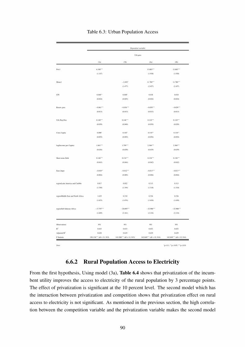
Table 6.3: Urban Population Access

Dependent variable:

Urb perc

(3a) (3b) (4a) (4b)

Priv1 6.348∗∗∗ 13.883∗∗∗ 13.883∗∗∗

(1.147) (1.938) (1.938)

Mono1 −2.492∗ 11.780∗∗∗ 11.780∗∗∗

(1.477) (2.457) (2.457)

CPI 0.048∗∗ 0.048∗ 0.018 0.018

(0.024) (0.025) (0.024) (0.024)

Renew perc −0.061∗∗∗ −0.054∗∗∗ −0.059∗∗∗ −0.059∗∗∗

(0.013) (0.013) (0.013) (0.013)

Urb Pop Perc 0.140∗∗∗ 0.146∗∗∗ 0.110∗∗∗ 0.110∗∗∗

(0.039) (0.040) (0.039) (0.039)

Cons Capita 0.098∗ 0.102∗ 0.110∗∗ 0.110∗∗

(0.055) (0.055) (0.054) (0.054)

log(Income per Capita) 1.841∗∗∗ 1.759∗∗∗ 2.384∗∗∗ 2.384∗∗∗

(0.636) (0.650) (0.639) (0.639)

Short term Debt 0.146∗∗∗ 0.134∗∗∗ 0.136∗∗∗ 0.136∗∗∗

(0.043) (0.044) (0.042) (0.042)

Ener Impo −0.010∗∗ −0.012∗∗∗ −0.013∗∗∗ −0.013∗∗∗

(0.004) (0.005) (0.004) (0.004)

regionLatin America and Caribbe 0.817 0.052 0.313 0.313

(1.330) (1.354) (1.318) (1.318)

regionMiddle East and North Africa 1.635 0.210 0.236 0.236

(1.623) (1.674) (1.630) (1.630)

regionSub-Saharan Africa −17.797∗∗∗ −20.895∗∗∗ −22.988∗∗∗ −22.988∗∗∗

(1.849) (2.161) (2.124) (2.124)

Observations 951 951 951 951

R2 0.643 0.633 0.652 0.652

Adjusted R2 0.630 0.619 0.639 0.639

F Statistic 150.136∗∗∗ (df = 11; 915) 143.288∗∗∗ (df = 11; 915) 142.849∗∗∗ (df = 12; 914) 142.849∗∗∗ (df = 12; 914)

Note: ∗p<0.1; ∗∗p<0.05; ∗∗∗p<0.01

6.6.2 Rural Population Access to Electricity

From the first hypothesis, Using model (3a), Table 6.4 shows that privatization of the incum-bent utility improves the access to electricity of the rural population by 3 percentage points.The effect of privatization is significant at the 10 percent level. The second model which hasthe interaction between privatization and competition shows that privatization effect on ruralaccess to electricity is not significant. As mentioned in the previous section, the high correla-tion between the competition variable and the privatization variable makes the second model

90

less reliable.From the second hypothesis, Using model (3b) and in this case with the competition vari-

able, Table 6.4 shows that if the incumbent utility is a monopoly, this reduces the access toelectricity of the rural population by 2 percentage points. The competition variable is signifi-cant at 95 percent level. The negative correlation in the presence of a monopoly is consistentwith economic theory on the disadvantages of a monopoly. A country in Sub-Saharan Africasees a decline of 45 percentage points in rural electricity access, this is the largest amongstall the economic region. A country in Latin America on average faces a decline of 8 percentin access to rural electricity. Latin America and Sub Saharan Africa house some of the leastdeveloped countries and this is highlighted by the low levels of rural access to electricity inboth regions. There is a negative correlation with CPI; as the cost of living increases as indi-cated by the CPI there is a heavier burden on the rural consumer’s whose levels of income arelow in comparison to the urban population. Also, the rural economy depend on remittancesfrom the urban population, if the cost of living is rising there is a decline in disposable incometherefore reducing the income of the rural population. The other variables like, Income perCapita, Energy Imports, CPI , Renewable Energy, have correlations that are consistent with thecorrelations with urban access to electricity.

91

Table 6.4: Rural Population Access

Dependent variable:

Rural perc

(3a) (3b) (4a) (4b)

Priv1 3.555∗∗ 0.033 0.033

(1.691) (2.886) (2.886)

Mono1 −5.532∗∗∗ −5.499 −5.499

(2.138) (3.653) (3.653)

CPI −0.202∗∗∗ −0.188∗∗∗ −0.188∗∗∗ −0.188∗∗∗

(0.035) (0.036) (0.036) (0.036)

Renew perc −0.115∗∗∗ −0.116∗∗∗ −0.116∗∗∗ −0.116∗∗∗

(0.019) (0.019) (0.019) (0.019)

Urb Pop Perc −0.126∗∗ −0.112∗ −0.112∗ −0.112∗

(0.058) (0.058) (0.059) (0.059)

Cons Capita 0.170∗∗ 0.165∗∗ 0.165∗∗ 0.165∗∗

(0.081) (0.081) (0.081) (0.081)

log(Income per Capita) 14.436∗∗∗ 14.180∗∗∗ 14.181∗∗∗ 14.181∗∗∗

(0.937) (0.942) (0.952) (0.952)

Ener Impo −0.024∗∗∗ −0.023∗∗∗ −0.023∗∗∗ −0.023∗∗∗

(0.007) (0.007) (0.007) (0.007)

Short term Debt 0.234∗∗∗ 0.238∗∗∗ 0.238∗∗∗ 0.238∗∗∗

(0.063) (0.063) (0.063) (0.063)

regionLatin America and Caribbe −7.414∗∗∗ −7.185∗∗∗ −7.184∗∗∗ −7.184∗∗∗

(1.960) (1.963) (1.965) (1.965)

regionMiddle East and North Africa 0.856 1.506 1.506 1.506

(2.387) (2.423) (2.424) (2.424)

regionSub-Saharan Africa −41.086∗∗∗ −38.661∗∗∗ −38.666∗∗∗ −38.666∗∗∗

(2.721) (3.127) (3.158) (3.158)

Observations 941 941 941 941

R2 0.794 0.795 0.795 0.795

Adjusted R2 0.786 0.787 0.787 0.787

F Statistic 317.741∗∗∗ (df = 11; 905) 318.744∗∗∗ (df = 11; 905) 291.859∗∗∗ (df = 12; 904) 291.859∗∗∗ (df = 12; 904)

Note: ∗p<0.1; ∗∗p<0.05; ∗∗∗p<0.01

6.6.3 System Losses

From Table 6.5 we reject the hypotheses that both privatization and competition reduces thesystem losses on the electricity grid. This is because the coefficients for competition and priva-tization are not statistically significant. Even though we reject the hypotheses for system losses,the models provide insights on other factors that influences system losses on the electricity grid.Using the first model with either privatization or competition variable, the insights derived fromthis model is useful in deriving policies that help minimize system losses. Urban population is

92

positively correlated with system losses; as the population in urban areas increases, there is anincrease in demand. In order to meet this demand utilities have to produce more energy. If thereare no changes in the grid structure the distribution and transmission of more energy results inhigher system losses. Renewable energy is negatively correlated to system losses; renewablesources requires the improvement of the electric grid or results in the creation of mini grids,these two factors help reduce the system losses on the grid. Income per Capita is negativelycorrelated with system losses; this variable can be used as a measure of prosperity, thereforeas the prosperity of a country increases their system losses decreases. A prosperous nation caninvest in improvements of the electric grid therefore minimizing system losses. It should benoted that there are weaknesses in using income per capita as a measure of prosperity, how-ever, this assumption is sufficient for the purposes of this study. Energy imports are negativelycorrelated with system losses; as the imports increases the exports decreases, this reduces thelosses incurred during transmission and distribution as the losses due to imports are accountedfor by the exporting country. This analyses also shows that the economic region of a coun-try matters in accounting for system losses, as show by both tables, countries in Sub-SaharanAfrica have the highest system losses while European countries have the lowest system losses;the differences in economic development is captured by this variable. The highly developedregions can afford better infrastructure that results in reduced system losses while developingregion like Sub-Saharan Africa face a huge infrastructure deficiency which leads to increasedsystem losses. Policy makers in these regions should recognize the urgent need for developinginfrastructures for efficient distribution of electricity.

93

Table 6.5: System Losses Results

Dependent variable:

Syst Loss

(1) (2) (3) (4)

Priv1 0.258 −1.363 −1.363

(0.703) (1.228) (1.228)

Mono1 −1.071 −2.467 −2.467

(0.877) (1.533) (1.533)

CPI 0.003 0.006 0.008 0.008

(0.015) (0.015) (0.015) (0.015)

Renew perc −0.018∗∗ −0.019∗∗ −0.019∗∗ −0.019∗∗

(0.008) (0.008) (0.008) (0.008)

Urb Pop Perc 0.051∗∗ 0.053∗∗ 0.055∗∗ 0.055∗∗

(0.024) (0.024) (0.024) (0.024)

Urb perc 0.031 0.033 0.040 0.040

(0.025) (0.024) (0.025) (0.025)

Rural perc 0.017 0.015 0.012 0.012

(0.016) (0.016) (0.017) (0.017)

log(Income per Capita) −3.666∗∗∗ −3.692∗∗∗ −3.720∗∗∗ −3.720∗∗∗

(0.422) (0.423) (0.423) (0.423)

Ener Impo −0.015∗∗∗ −0.014∗∗∗ −0.014∗∗∗ −0.014∗∗∗

(0.003) (0.003) (0.003) (0.003)

Short term Debt 0.076∗∗∗ 0.078∗∗∗ 0.078∗∗∗ 0.078∗∗∗

(0.026) (0.026) (0.026) (0.026)

regionLatin America and Caribbe 0.056 0.169 0.120 0.120

(0.812) (0.811) (0.812) (0.812)

regionMiddle East and North Africa −3.988∗∗∗ −3.699∗∗∗ −3.693∗∗∗ −3.693∗∗∗

(0.968) (0.984) (0.984) (0.984)

regionSub-Saharan Africa 0.691 1.502 1.756 1.756

(1.247) (1.392) (1.411) (1.411)

Observations 941 941 941 941

R2 0.293 0.294 0.295 0.295

Adjusted R2 0.265 0.266 0.266 0.266

F Statistic 31.171∗∗∗ (df = 12; 904) 31.330∗∗∗ (df = 12; 904) 29.023∗∗∗ (df = 13; 903) 29.023∗∗∗ (df = 13; 903)

Note: ∗p<0.1; ∗∗p<0.05; ∗∗∗p<0.01

6.6.4 Interaction Effects

In order to understand the effects of privatization and competition on the regional level, weinteract these effects with the region variable. The interaction effect gives insight into thedifferential impact on privatization and competition relative to the reference group. The in-teraction variables are chosen based on literature and or other factors. A consistent them of

94

this dissertation is understanding electricity markets in developing countries, specifically Sub-Saharan Africa. It follows from this interest that the interaction effect is specified as shownbelow;

per fit = αi + γt +β1(Privit)+β3(Privit ∗ region)+θ(Xit)+ εit (7a)

An equivalent version of (7a) is created for the competition variable.However, a consistent theme of this dissertation is to understand there is a stronger inter-

est on the effects of privatization and competition in Sub-Saharan Africa. In order to furtheranalyze the interaction effects on this region, the following model is created;

per fit = αi+ γt +β1(Privit)+β3(Privit ∗ region = SSA)+β4(Privit ∗ region)θ(Xit)+εit (7b)

The interaction effect provides information on the effect of privatization and competitionbased on the geographical region of the country. Controlling for the interaction effect is tomodulate the effects of geographical location. From (7a) and Table 6, privatization increasesurban access to electricity in Sub Saharan Africa and Europe by 14 %, the effects of priva-tization on urban access to electricity in the Latin America and Middle East region can beunderstood by combining the regional interaction. For Latin America, this interaction effect,(β4∗region+beta1)Priv ,is 5% , while the interaction effect for Middle East is -1%. The priva-tization effect is not significant for rural access , however the interaction effect for Middle Eastis significant, resulting in an effect of 16%. The rest of the explanatory factors have similarexplanations as already given in the sections above.

In order to understand the interaction effect on Sub Saharan Africa, model (7b) which makesthe region equal to Sub-Saharan Africa is used. From this model the interaction effect is givenby , (β3 ∗ region+beta1)∗Priv , which is 14% for urban access , this is consistent with model(7a). For rural access, the privatization interaction has -1% on access in rural populations. Theresults in Table 7.6 and Table 7.7 shows that model (7a) and (7b) are equivalent. The generalinsight emerging from the interaction effects analysis is that privatization and competition havea strong impact in Sub-Saharan Africa and the Middle East. Intuitively, both regions have thelowest levels privatization of utilities and lower access rates to electricity. Introducing privatiza-tion in these markets should analytically improve the levels of access. Another interpretation ofthese findings is that since Sub Saharan Africa has lower privatization and competition levels,its electricity markets are not economically efficient and one consequence of this is reflectedin the lower levels of electricity access in this region. This also provides a policy change op-portunity in the poor performing regions. Creating policies that encourage privatization andcompetition in Sub-Saharan Africa should be a priority to policy makers in this region.

The analysis for privatization effects can be repeated for the competition effects, the sum-mary of this analysis is shown in Table 7.8

95

Table 6.6: Region* Privatization Interaction

Dependent variable:

Urb perc Rural perc Syst Loss

(1) (2) (3)

Priv1 14.051∗∗∗ −0.863 −1.655

(1.920) (2.835) (1.220)

CPI 0.006 −0.152∗∗∗ 0.015

(0.025) (0.037) (0.015)

Renew perc −0.060∗∗∗ −0.111∗∗∗ −0.018∗∗

(0.013) (0.019) (0.008)

Urb Pop Perc 0.104∗∗∗ −0.087 0.058∗∗

(0.040) (0.059) (0.024)

Cons Capita 0.119∗∗ 0.132

(0.054) (0.081)

Urb perc 0.053∗∗

(0.026)

Rural perc 0.001

(0.017)

log(Income per Capita) 2.706∗∗∗ 13.021∗∗∗ −3.871∗∗∗

(0.661) (0.977) (0.425)

Ener Impo −0.016∗∗∗ −0.010 −0.011∗∗∗

(0.005) (0.007) (0.003)

Short term Debt 0.141∗∗∗ 0.224∗∗∗ 0.074∗∗∗

(0.042) (0.062) (0.026)

regionLatin America and Caribbe 10.120∗∗∗ −5.906 −0.651

(2.904) (4.284) (1.792)

regionMiddle East and North Africa 14.189∗∗∗ −11.691∗∗∗ −8.214∗∗∗

(2.909) (4.292) (1.815)

regionSub-Saharan Africa −10.838∗∗∗ −45.916∗∗∗ −1.388

(2.276) (3.358) (1.528)

Priv1:regionLatin America and Caribbe −9.498∗∗∗ −2.560 0.352

(2.788) (4.109) (1.705)

Priv1:regionMiddle East and North Africa −15.271∗∗∗ 17.688∗∗∗ 5.750∗∗∗

(3.046) (4.492) (1.939)

Observations 951 941 941

R2 0.654 0.799 0.301

Adjusted R2 0.640 0.791 0.271

F Statistic 132.604∗∗∗ (df = 13; 913) 276.497∗∗∗ (df = 13; 903) 27.696∗∗∗ (df = 14; 902)

Note: ∗p<0.1; ∗∗p<0.05; ∗∗∗p<0.01

96

Table 6.7: Region* Privatization Interaction with Sub-Saharan Africa Specification

Dependent variable:

Urb perc Rural perc Syst Loss

(1) (2) (3)

Priv1 −1.220 16.825∗∗∗ 4.096∗∗∗

(2.243) (3.305) (1.388)

CPI 0.006 −0.152∗∗∗ 0.015

(0.025) (0.037) (0.015)

Renew perc −0.060∗∗∗ −0.111∗∗∗ −0.018∗∗

(0.013) (0.019) (0.008)

Urb Pop Perc 0.104∗∗∗ −0.087 0.058∗∗

(0.040) (0.059) (0.024)

Cons Capita 0.119∗∗ 0.132

(0.054) (0.081)

Urb perc 0.053∗∗

(0.026)

Rural perc 0.001

(0.017)

log(Income per Capita) 2.706∗∗∗ 13.021∗∗∗ −3.871∗∗∗

(0.661) (0.977) (0.425)

Ener Impo −0.016∗∗∗ −0.010 −0.011∗∗∗

(0.005) (0.007) (0.003)

Short term Debt 0.141∗∗∗ 0.224∗∗∗ 0.074∗∗∗

(0.042) (0.062) (0.026)

region == ”Sub-Saharan Africa” −26.109∗∗∗ −28.228∗∗∗ 4.363∗∗

(2.651) (3.907) (1.694)

regionLatin America and Caribbe −5.152 11.782∗∗ 5.100∗∗∗

(3.208) (4.728) (1.962)

regionMiddle East and North Africa −1.083 5.998∗∗ −2.464∗∗

(1.766) (2.603) (1.076)

Priv1:region == ”Sub-Saharan Africa” 15.271∗∗∗ −17.688∗∗∗ −5.750∗∗∗

(3.046) (4.492) (1.939)

Priv1:regionLatin America and Caribbe 5.773∗ −20.248∗∗∗ −5.398∗∗∗

(3.129) (4.613) (1.942)

Observations 951 941 941

R2 0.654 0.799 0.301

Adjusted R2 0.640 0.791 0.271

F Statistic 132.604∗∗∗ (df = 13; 913) 276.497∗∗∗ (df = 13; 903) 27.696∗∗∗ (df = 14; 902)

Note: ∗p<0.1; ∗∗p<0.05; ∗∗∗p<0.01

97

Table 6.8: Region* Competition Interaction

Dependent variable:

Urb perc Rural perc Syst Loss

(1) (2) (3)

Mono1 0.138 −16.754∗∗∗ −3.903∗∗∗

(2.302) (3.298) (1.383)

CPI 0.039 −0.153∗∗∗ 0.012

(0.025) (0.036) (0.015)

Renew perc −0.055∗∗∗ −0.111∗∗∗ −0.018∗∗

(0.013) (0.019) (0.008)

Urb Pop Perc 0.141∗∗∗ −0.090 0.056∗∗

(0.040) (0.058) (0.024)

Cons Capita 0.109∗ 0.133∗

(0.056) (0.081)

Urb perc 0.043∗

(0.025)

Rural perc 0.006

(0.017)

log(Income per Capita) 2.013∗∗∗ 13.070∗∗∗ −3.833∗∗∗

(0.673) (0.967) (0.425)

Ener Impo −0.015∗∗∗ −0.010 −0.011∗∗∗

(0.005) (0.007) (0.003)

Short term Debt 0.137∗∗∗ 0.224∗∗∗ 0.075∗∗∗

(0.044) (0.062) (0.026)

region == ”Sub-Saharan Africa” −14.976 −51.519∗∗∗ 0.905

(11.456) (16.413) (6.801)

regionLatin America and Caribbe 0.313 −8.422∗∗∗ −0.229

(1.371) (1.970) (0.824)

regionMiddle East and North Africa −0.836 5.980∗∗ −2.533∗∗

(1.817) (2.603) (1.076)

Mono1:region == ”Sub-Saharan Africa” −8.351 23.147 3.006

(11.629) (16.661) (6.885)

Mono1:regionLatin America and Caribbe −4.621 20.154∗∗∗ 5.143∗∗∗

(3.215) (4.607) (1.934)

Observations 951 941 941

R2 0.634 0.799 0.299

Adjusted R2 0.619 0.791 0.270

F Statistic 121.469∗∗∗ (df = 13; 913) 276.520∗∗∗ (df = 13; 903) 27.510∗∗∗ (df = 14; 902)

Note: ∗p<0.1; ∗∗p<0.05; ∗∗∗p<0.01

98

6.7 Conclusions

This study provides an empirical analysis of the effects of privatization and competition onthe performance of electricity markets. Using the linear model, this study shows the effectsof privatization and competition on a access to electricity and system losses. While there arelimitations to this analysis, it provides a framework for effectively measuring the performancesof utilities. This analysis also provides insight on other determinants of performance of electricutilities; this is especially important for policy makers in terms of creating instruments that canimprove the performance of electric utilities.This analysis shows that privatization of utilitiesand the introduction of competition improves the levels of access of electricity amongst therural and the urban population. However, these two factors do not have a significant effecton system losses. The results show that system losses are directly correlated with the overallprosperity of a country as shown by variables that are directly correlated with system losses.Access to electricity is one of the main indicators of economic growth, and the results show thatSub-Saharan Africa and Latin America, two of the least developed regions, have lower levels ofelectricity access in comparison to other economic regions. The results show a decrease of 20percentage points for urban access and 40 percentage decrease in rural access if a country is inSub-Saharan Africa. These indicators calls for a need in economic reforms for countries in Sub-Saharan Africa in order to increase accessibility of electricity in this region. The regional effectsprovides a great contrast between regions that have adopted privatization and competition toregions that are still in the process of implementing the two; Europe and Sub-Saharan Africaprovides a great example of this contrast. European electricity markets are liberalized and thereis both public and private participation on the market, while the Sub-Saharan African marketsare heavily dominated by government control with the majority of the markets having one singledominant utility player. A juxtaposition of these two markets shows that markets in developingeconomies under perform when compared to European markets in terms of access to electricityand system losses. The results presented in this study are consistent with economic theoryand other studies on economic development. The analysis presented is an effective way ofmeasuring the performance of electricity markets. The econometric approach provides policymakers with empirical evidence on the policy changes.

99

Chapter 7

Conclusions and Future Work

7.1 Conclusions

The majority of developed countries have made the shift from monopoly designs to competi-tive markets that allows for higher reliability and improved quality of service. The majority ofdeveloping countries, especially in Sub Saharan Africa have a monopoly or semi-deregulatedmarket structure. Most developed countries have on average 100 % electricity access for boththe urban and rural populations. Developing countries still lag in the levels of electricity accessfor both the urban and rural populations, on average the rural populations have a much loweraccess rate compared to the urban population. This is due to the poor infrastructure distributionlevel, most of the utility infrastructure is heavily concentrated in urban areas. There are countryspecific initiatives to improve the infrastructure and access levels, for example, South Africaand Zimbabwe have a rural electrification program that is meant to accelerate infrastructure de-velopment to rural parts of the country. The first study presented an inter-temporal frameworkfor analyzing the pricing path that can be employed by a competitive incumbent and a com-petitive market entrant in the electricity markets of developing economies. It provided a policyframework that is consistent with the policy needs in developing economies i.e encouragingparticipation of private players in the electricity markets and provided a profitable frameworkthat can be implemented by new investors. This study also provided a robust extension of thetheoretical framework introduced by Chisari. Market players employ an increasing pricing paththat converge to the steady state prices of competitors.

The calls for a cleaner earth and the advancements in technologies used to extract and userenewable energy sources have changed energy economics. There is a need for an active inves-tigation into how to efficiently reduce the emissions levels from electricity generation in orderto minimize environmental damage and increase consumer welfare. These models can varyfrom place to place depending on consumption levels and energy sources available. Pigou-vian taxes and Tradable permits have been used to reduce the emissions of greenhouse gasesto efficient levels. This study focused on electricity markets in developing that are dominated

100

by conventional energy sources and a need to leverage the competitiveness of firms providingenergy from renewable sources. Using a duopoly market; there are two levels of strategic in-teractions introduced; the pricing competition between the market players and the optimal taxlevel introduced by the policymaker. This project showed that introducing a tax on the price ofthe conventional fuel allowed the entrant utility to be competitive in terms of marked prices.

The focus of the first two studies is on a policy level. However, it is important to measure theeffects of these policy changes using some objective benchmarks. This allows the policymakerto evaluate the effects of the old and new policies. A cross country or cross geographical studyallows the policy maker to have a comparative view of the performance of their electricitymarkets relative to other markets in their region or in other regions. This objective measureallows for critical analysis of the policies implemented in individual countries or regions.Thelast study provides an empirical analysis of the effects of privatization and competition on theperformance of electricity markets. Using the linear model, this study shows the effects ofprivatization and competition on a access to electricity and system losses. While there arelimitations to this analysis, it provides a framework for effectively measuring the performancesof utilities. This analysis also provides insight on other determinants of performance of electricutilities; this is especially important for policy makers in terms of creating instruments that canimprove the performance of electric utilities.

7.2 Future Work

Policy makers in developed and developing economies often regulate the prices of electricutilities. The goal of price regulation is to protect consumers from predatory pricing by utilities.In developing economies where the electricity markets are dominated by monopolies, pricingregulation can protect consumers from monopoly pricing. However certain pricing caps e.gdynamic pricing cap, allows an entry deterring incumbent firm to set its prices such that anpotential entrant is not profitable upon entry. Future work will focus on a strategic interactionbetween an incumbent firm, a policy maker and a potential entrant. The goal is to strategicallyplace the policy maker to minimize entry deterrence on the part of the incumbent by transferringa subsidy to the potential entrant to reduce its entry costs. The model presented in Chapter 4can be extended to look at the Stackelberg set up, this will allow the incumbent firm to be theleader while the entrant firm is the follower in price setting. This can present interesting insightin the analysis of developing markets. The strategic interaction in Chapter 5 can be expandedto cover the stochastic nature of demand functions. That will provide a detailed analysis forfirms to contrast with the deterministic solution. In both chapters numerical examples can addmore insight on the pricing strategies provided by the analytical solutions provided. The workpresented in this dissertation provides a lot of avenues for further analysis of electricity marketsin developing economies.

101

7.3 Publications

1. Matenga.Z, Fedderke.J and Terpenny.J, 2018, ”Pricing Dynamics of Electricity in Priva-tized Markets with Underdeveloped Networks” IISE Conference

2. Matenga.Z, Fedderke.J and Terpenny.J, 2019, ”Optimal Taxing Strategy to Increase Com-petitiveness of Green Utility Suppliers: A Theoretical Framework” Accepted IISE Con-

ference

3. Matenga.Z, Fedderke.J and Terpenny.J, 2018, ”Pricing Dynamics of Electricity in Priva-tized Markets with Underdeveloped Networks” under review Energy Economics

4. Matenga.Z, Fedderke.J and Terpenny.J, 2019, ”Optimal Taxing Strategy to Increase Com-petitiveness of Green Utility Suppliers: A Theoretical Framework” under review Energy

Policy

5. Matenga.Z, Fedderke.J and Terpenny.J, TBD, ”Measuring the effects of Competition andPrivatization in Electricity Markets: An Econometric Approach” to be submitted Energy

Policy

102

Bibliography

[1] Rothwell.G and Gomez.T, 2003, ”Electricity Economics: Regulation and Deregula-tion,”IEEE Power Engineering Society

[2] Chisari.O and Kessides.I, 2009, ”Pricing Dynamics of Network Utilities in DevelopingCountries,” Review of Network Economics, vol(8)Issue 3.

[3] Buchanan.J and Tullock.G, 1962,”The Calculus of Consent: Logical Foundations of Con-stitutional Democracy,” University of Michigan

[4] Stern.J and Holder.S , 1999, ”Regulatory Governance: Criteria for Assessing the Perfor-mance of Regulatory Systems”

[5] Transparency International, 2017, Corruption Perceptions Index

[6] World Bank(2008) Sustainable Infrastructure Action Plan.

[7] World Energy Council, 2001, Pricing Energy in Developing Countries.

[8] Modise.D and Mahotas.V, 2009,”The South African Energy Sector,” Department of Energy.

[9] Aschauer D.A, 1989, ”Is Expenditure Productive?”Journal of Monetary Eco-

nomics,23:177-200

[10] Estache.A , 2005, ”What do we know about Sub-Saharan Africa’s Infrastructure and theImpact of the 1990’s Reforms?”Mimeo, World Bank, Washington DC.

[11] Leipziger.D , Fay.M, Wodon.Q and Yepes.T, 2003,”Achieving the Millenium Develop-ment Goals : The Role of Infrastructure”Policy Research Working Paper World Bank,Washington DC.

[12] Bogetic .Z and Fedderke.J, 2006,”Forecasting Investments Needs in South Africa’s Elec-tricity and Telecom Sectors,”South African Journal of Economics,vol74:3

[13] Calderon.C and Serven . L, 2008, ”Infrastructure and Economic Development in Sub-Saharan Africa,”Policy Research Working Paper No 4712,World Bank, Washington DC.

103

[14] Holland.M , 2017, ”Health impacts of coal fired power plants in South Africa, ”Ground-

work(South Africa)

[15] Norregaard.J and Reppelin-Hill.V, 2000, ”Taxes and Tradable Permits as Instrument forControlling Pollution: Theory and Practice,” IMF Working Paper WP/00/13.

[16] Heerden .J, Gerlagh.R, Blignaut.J,Horridge.M , Hess.S, Mabugu.R and Mabugu.M , 2006,”Searching for Triple Dividends in South Africa: Fighting C02 pollution and poverty whilepromoting growth,” IMF Working Paper WP/00/13.

[17] Kamien, Morton.I and Schwartz.N, 1981, ”Dynamic Optimization: The Calculus of Vari-ations and Optimal Control in Economics and Management,” New York: North-Holland

[18] Dorfman.R, 1969, ”An Economic Interpretation of Optimal Control Theory,” The Ameri-

can Economic Review, Vol. 59, pp. 817-831

[19] Buchanan. J, 1969, ”External Diseconomies, Corrective Taxes and Market Structure,”American Economic Review,Vol.59,pp. 139-47

[20] Requate.T, 1993, ”Pollution Control in a Cournot Duopoly via Taxes or Permits,”Journal

of Economics,Vol.58, pp255-91

[21] Koustaal. P, 1997, ”Economic Policy and Climate Change: Tradable Permits for ReducingCarbon Emissions,” Cheltenham,UK: Edward Elgar

[22] Xepapadeas.A, 1997, ”Advanced Principles in Environmental Policy,” Cheltenham,UK:Edward Elgar

[23] Gaskins.D, 1970, ”Dynamic Limit Pricing: Optimal Pricing under Threat of Entry.” Jour-

nal of Economic Theory 3: 306-322

[24] Thisse.J.F, 1972, ”Un modele dynamique de la firme avec differenciation du prodiut”Recherches Economiques de Louvain,no.1, April, 3-16.

[25] Jacquemin,A.P, 1973, ”Optimal control and advertising policy.” Metroeconomica 25, 200-207.

[26] Horsky.D , 1977, ”Empirical analysis of optimal advertising policy .” Management Sci-

ence 23, no.10,1037-1049.

[27] Bensoussan. A , Bultez.A and Naert. P , 1978, ”Leader’s dynamic marketing behaviorin oligopoly, in: A. Bensoussan, P.R. Kleindorfer and C.S. Tapiero, eds,” Applied optimal

control(North-Holland , Amsterdam)123-145.

[28] Gilbert.R , 1989, ”Mobility barriers and the value of incumbency.” Handbook of Industrial

Organization, vol 1.North-Holland, Amsterdam , pp.475-535.

104

[29] Jamison.M,2005, ”Rate of Return: Regulation,”Public Utility Research Center, University

of Florida

[30] Brock.W and Dechert .W , 1985, ”Dynamic Ramsey Pricing.” International Economic

Review 26(3): 569-591

[31] Hamermesh.D and Pfann.G , 1996, ” Adjustment costs in Factor Demand.” Journal of

Economic Literature XXXIV:1264-1292

[32] Zaccour.G, 2013, ”Differential Games in the Economics and Management of Pollution:A Tutorial,”GERAD, HEC Montreal, Canada

[33] Basar.T and Olsder.G, 1999, ”Dynamic Noncooperative Game Theory”Classics in Ap-

plied Mathematics: 2nd Edition

[34] Eliashberg.J and Steinberg. R, 1987, ”Marketing-production decisions in an industrialchannel of distribution,”Management Science,33(8):981-1000

[35] Desai. V.S, 1992, ”Market-production decisions under independent and integrated channelstructure, ” Annals of Operations Research, 34:275-306

[36] Desai. V.S, 1996,”Interactions between members of a marketing-production channel un-der seasonal demand,”European Journal of Operations Research,90:115-141

[37] Chintagunta.P and Jain.D, 2002, ”A dynamic model of channel member strategies formarketing expenditures,”Marketing Science, 11(2):168-188

[38] Frutcher. G and Messinger.P , 2003, ” Optimal management of fringe entry over time.”Journal of Economic Dynamics and Control28 pp 445-446.

[39] Kogan.K and Tapiero C.S, 2007, ”Supply Chain Games: Operations Management andRisk Valuation,”Springer.New York.

[40] He.X and Sethi S.P , 2008, ”Dynamic slotting and pricing decisions in a durable productsupply chain.”Journal of Optimization Theory and Applications 134(8)

[41] Fanokoa .S.P , Telahigue.I and Zaccour G, 2010, ”Buying cooperation in an asymmetricenvironmental differential game,”Journal of Economic Dynamics and Control

[42] Novak.A.J , Feichtinger .G and Leitmann .G, 2010, ”A differential game related to terror-ism: Nash and Stackelberg Strategies”

[43] Anorld. M and Narciso. G, 2008, ”Services Inputs and Firm Productivity in Sub-SaharanAfrica: Evidence from Firm level Data,” Journal of African Economies 17(4)

105

[44] Bogetic. Z and Fedderke.W ,2006, ”Forecasting Investment Needs in South Africa’s Elec-tricity and Telecommunications Sectors.” South African Journal of Economics EconomicSociety of South Africa,vol.74(3): 557-574

[45] Breeze. P, 2010, ”The Cost of Power Generation,” Business Insights

[46] Brock.W and Dechert. W , 1985, ”Dynamic Ramsey Pricing.” International Economic

Review 26(3): 569-591

[47] Buchanan. J, 1969, ”External Diseconomies, Corrective Taxes and Market Structure,”American Economic Review,Vol.59,pp. 139-47

[48] Chiang. A, 1992, ”Elements of Dynamic Optimization.” Mcgraw-Hill. Inc

[49] Chisari. O and Kessides. I, 2009, ”Pricing Dynamics of Network Utilities in DevelopingCountries,” Review of Network Economics, vol(8) Issue 3 .

[50] Eberhard. A and Gratwick.K, 2011, ”IPP’s in Sub-Saharan Africa: Determinants of Suc-cess,”Energy Policy(39) 5541-5549

[51] Eberhard. A, Gratwick.K, Morella. E and Antmann P, 2016, ”Independent Power Projectsin Sub-Saharan Africa.” The World Bank

[52] El-Hawary. M, 1995, ”Electrical Power Systems,” John Wiley & Sons, Inc

[53] El-Hawary. M. E and Mansour . S. Y, “Performance evaluation of parameter estimationalgorithms for economic operation of power systems”, IEEE Transactions on Power Appa-

ratus and Systems, Vol. PAS-101, pp. 574–82, 1982.

[54] Escribano. A, Gausch. J and Pena. J, 2009, ”Assessing the Impact of Infrastructure Qualityon Firm Productivity in Africa,” Africa Infrastructure Country Diagnostic, The World Bank

[55] Gaskins. D, 1970, ”Dynamic Limit Pricing: Optimal Pricing under Threat of Entry.” Jour-

nal of Economic Theory 3: 306-322

[56] Gilbert. R, 1989, ”Mobility barriers and the value of incumbency .” Handbook of Indus-

trial Organization, vol 1.North-Holland , Amsterdam , pp.475-535.

[57] Hamermesh. D and Pfann. G , 1996, ” Adjustment costs in Factor Demand.” Journal of

Economic Literature XXXIV:1264-1292

[58] Heerden. J, Gerlagh. R, Blignaut.J, Horridge.M , Hess.S, Mabugu. R and Mabugu. M ,2006, ”Searching for Triple Dividends in South Africa: Fighting C02 pollution and povertywhile promoting growth,” IMF Working Paper WP/00/13.

106

[59] Hemamalini .S and Simon .S.P, 2010, “Artificial bee colony algorithm for economic loaddispatch problem with non-smooth cost functions”, Electric Power Components and Sys-

tems, Vol. 38, pp. 786–803

[60] Holland. M, 2017, ”Health Impacts of Coal Fired Power Plants in South Africa,” Ground-

work, Health Care Without Harm

[61] Joseph. K. L , 2010, ”The Politics of Power: Electricity Reform in India,” Energy Policy

38, 503-511

[62] Koustaal.P, 1997, ”Economic Policy and Climate Change: Tradable Permits for ReducingCarbon Emissions,” Cheltenham, UK: Edward Elgar

[63] Mangasarian. O , 1966, ”Sufficient Conditions for the Optimal Control of Nonlinear Sys-tems.” SIAM Journal on Control 4: 139-152

[64] Modise. D and Mahotas. V, 2009, ”The South African Energy Sector,” Department of

Energy.

[65] Northeast Group, 2017, ”Electricity Theft and Non-Technical Losses: Global Markets,Solutions and Vendors,” Northeast Group, LLC

[66] Norregaard. J and Reppelin-Hill. V, 2000, ”Taxes and Tradable Permits as Instrument forControlling Pollution: Theory and Practice,” IMF Working Paper WP/00/13.

[67] Pontryagin. L, Boltyanskii. V , Gamkrelidze .R and Mishchenko. E, 1962, ”The Mathe-matical Theory of Optimal Processes.” New York: Wiley

[68] Requate. T, 1993, ”Pollution Control in a Cournot Duopoly via Taxes or Permits,”Journal

of Economics,Vol.58, pp255-91

[69] Shoults. R. R and Mead. M. M,1984, “Optimal estimation of piece-wise linear incre-mental cost curves for EDC”, IEEE Transactions on Power Apparatus and Systems, Vol.PAS-103, pp. 1432–1438.

[70] Smith. T, 2004, ”Electricity Theft: a comparative analysis,” Energy Policy

[71] Taylor. F. J and Huang C. J, 1977, “Recursive estimation of incremental cost curves”,Computers and Electrical Engineering,

[72] Theerthamalai. A and Maheswarapu.S,2010, ”An effective non-terative ”λ -logic based”algorithm for economic dispatch of generators with cubic fuel cost function,” International

Journal of Electrical Power and Energy Systems,Vol 32,Issue 5 pp 539-542

[73] World Bank, 2008 , Sustainable Infrastructure Action Plan.

107

[74] World Energy Council, 2001, Pricing Energy in Developing Countries.

[75] Xepapadeas. A, 1997, ”Advanced Principles in Environmental Policy,”Cheltenham,UK:

Edward Elgar

[76] Zivic M, Milacic . A and Krsulja. M, 2012, ”A simplified model of quadratic cost functionfor thermal generators,” Annals and Proceedings of DAAAM International vol 23 2

[77] Iozzi.A, 2001, ” Strategic Pricing and Entry Deterrence under Price-cap Regulation” Jour-

nal of Economics, Vol.74(2001),No.3, pp 283-300

[78] Coyne.C and Coyne. R, 2015, ” The Economics of Price Control,”Flaws and Ceilings:

Price Controls and the Damage They Cause. IEA , UK

[79] Averch. H and Johnson .L, 1962, ”Behavior of the Firm Under Regulatory Constraint,”The American Economic Review, Vol. 52, No. 5, pp. 1052-1069

[80] Ndulu, B., S. O’Connell, R. Bates, P. Collier and C. Soludo ,2008a, ”The Political Econ-omy of Economic Growth in Africa 1960-2000” Vol. 1, Cambridge: Cambridge UniversityPress.

[81] Chisari. O and Kessides.I , 2009, ”Pricing Dynamics of Network Utilities in DevelopingCountries,” Review of Network Economics,vol(8) Issue 3.

[82] Fosu, A. K, R. Bates and A. Hoeffler , 2006, ”Institutions, Governance and EconomicDevelopment in Africa: An Overview,” Journal of African Economies, supplement, vol.15(1), pages 1-9.

[83] Vogelsang.I and Finsinger.J, 1979, ”A Regulatory Adjustment Process for Optimal Pric-ing by Multiproduct Monopoly Firms.”Bell Journal of Economics10:157-71

[84] Sappington, D.E.M, 1980, ”Strategic Firm Behavior under a Dynamic Regulatory Adjust-ment Process.”Bell Journal of Economics11:360-72

[85] Sappington, D.E.M and Sibey,D.S,1992, ”Strategic Nonlinear Pricing under Price-capRegulation.”Rand Journal of Economics23:1-19

[86] Armstrong.M and Vickers.J, 1993, ”Price Discrimination , Competition and Regula-tion”Journal of Industrial Economics XLI:335-59

[87] Bos.D and Nett.L , 1990, ”Privatization, Price Regulation, and Market Entry. An Asymet-ric Multistage Duopoly Model.”Journal of Economics51:221-57

[88] Law,P.J, 1997,”Welfare Effects of Pricing in Anticipation of Laspeyres Price-cap Regula-tion: An Example”Bulletin of Economic Research49:17-27.

108

[89] Foreman, R.D, 1995, ”Pricing Incentives under Price-cap Regulation.”Information Eco-

nomics and Policy7: 331-51

[90] Vickers.J and Yarrow.G, 1991, ”Economic Perspective on Privatization” American Eco-

nomic Asscociation Vol.5, No.2,111-132

[91] Ndulu.B, O’Connell.S, Bates.R, Collier.P and Soludo.C ,2008a, ” The Political Econ-omy of Economic Growth in Africa 1960-2000” Vol. 1, Cambridge: Cambridge UniversityPress.

[92] Littlechild.S, 1983, ”Regulation of British Telecom’s Profitability,”Report to the Secretary

of State Department, Department of IndustryLondon.

[93] Mathios A.D, Robinson.K, 1989, ”The Impact of Alternative Forms of State Regulationof AT&T on Direct-Dial, Long-Distance Telephone Rates,”Price-Cap Symposium,Rand

Journal of Economics 20 (No. 3, Autumn): 437–453.

[94] Tirole. J, 1988,”The Theory of Industrial Organization.”Cambridge, Mass: MIT Press.

[95] Liston.C, 1993, ”Price-Cap versus Rate of Return Regulation,”Journal of Regualtory Eco-

nomics Vol.5, issue 1, 25-48

[96] Zhang. Y, Kirkpatrick. C and Parker.D, 2008, ”Electricity Sector Reform in DevelopingCountries: An Econometric Assessment of the Effects of Privatization, Competition andRegulation” Journal of Regulatory Economics Vol 33,Issue 2,pp 159-178

[97] Vlahinic-Dizdarevic. N, 2011, ”The Effects of Privatization in Electricity Sector: TheCase of Southeast European Countries,”

[98] Kessides. I, 2012, ”The Impacts of Electricity Sector Reforms in Developing Coun-tries”The Electricity JournalVol 25, Issue 6,pp 79-88

[99] Ros. A, 1999, ”Does Ownership or Competition Matter? The Effects of Telecommunica-tions Reform on Network Expansion and Efficiency”Journal of Regulatory EconomicsVol15,Issue 1,pp 65-92

[100] Ramamurti.R, 1997, ”Testing the Limits of Privatization-Argentine Railroads,” World

Development, 25(12), 1973-93

[101] Hawdon.D, 1996, ”Performance of Power Sectors in Developing Countries-A Study ofEfficiency and World Bank Policy using Data Envelopment Analysis,”Surrey Energy Eco-

nomics Centre Discussion Paper 88.

[102] Galal .A, Jones.L, Tandon. P and Vogelsang.I, 1994, ”Welfare Consequences of SellingPublic Enterprises-An Empirical Analysis” The World Bank

109

[103] Boubakri .V and Cosset .J.C , 1998, ”The Financial and Operating Performance of NewlyPrivatized Firms: Evidence from Developing Countries”Journal of Finance,53(3), 1081-1110.

[104] Delfino.A and Casarin .A , 2001, ”The Reform of the Utilities Sector in Ar-gentina,”United Nations University World Institute for Development Economics Research

Discussion Paper No. 2001/74, June.

[105] Torero.M and Rekve.P, 1998, ”Privatization in Developing Countries: Lessons to beLearnt from the Mozambican Case,” Transformation,No.36,pp.73-92

[106] Dewenter.K.L and Malatesta .P.H, 2001, ”State-Owned and Privately-Owned Firms: AnEmpirical Analysis of Profitability, Leverage, and Labor Intensity,”American Economic

Review,91(1), 320-335.

[107] Bortolotti.B, Fantini.M and Siniscalco. D, 1998.”Regulation and Privatization: the Caseof Electricity,”Working Paper, Department of Economics and Finance,University of Turin.

[108] Pollit.M.G, 1997, ”The Impact of Liberalization on the Performance of the ElectricitySupply Industry: An International Survey,”The Journal of Energy Literature, 3(2),3-31

[109] Macedo.R,2000, ”Privatization and the Distribution of Assets in Brazil,”Washington

DC.: Inter-American Development Bank Research Department.

[110] Parker. D, 2002,”Economic Regulation: A Review of Issues”Annals of Public and Co-

operative Economics,73(4)

[111] Vickers.J and Yarrow.G, 1998, ”Privatization : An Economic Analysis,”London-

Cambridge MA, The MIT Press

[112] Lee.J.D, Park.S and Kim.T, 1999, ”Profit, Productivity, and Price Differential: An In-ternational Performance Comparison of the Nature Gas Transportation Industry,”Energy

Policy

[113] Villalong .B, 2000,”Privatization and Efficiency: Differentiating Ownership Effects fromPolitical , Organizational, and Dynamic Effects,”Journal of Economic Behaviour & Orga-

nization,42,43-74

[114] Estache. A, 2000, ”In Infrastructure for Development: Private Solutions and thePoor,”World Bank and ECARES, Universite Libre de Bruxelles

[115] Wood.R, 2004,”The Privatization of Public Utilities:What are the Gains? Why the Pop-ular Opposition?” unpublished manuscript

110

[116] Paredes.M,2001, ”Redistributive Impact of Privatization and the Regulation of Utilitiesin Chile.” World Institute for Development Economics Research

[117] Wallstein. S,2001,”An Econometric Analysis of Telecom Competition, Privatization,Regulation in Africa and Latin America”

[118] Garrigou. A,2017, ”The impacts of bringing electricity to rural and vulnerable popula-tions,”The Beam

[119] World Bank,2017b, ”State of Electricity Access Report,” Washington: World Bank

[120] Scott.A,2017, ”Why Wait? Seizing the Energy Access Dividend,”Sustainable Energy

for All and Power For All

[121] Tallapragada.P, Shkaratan.M, Izaguirre.A, Helleranta.J,Rahman.S and Bergman.S, 2009,”Monitoring Performance of Electric Utilities: Indicators and Benchmarking in Sub-Saharan Africa”World Bank

[122] Matenga.Z, Fedderke.J and Terpenny.J, 2018, ”Pricing Dynamics of Electricity in Priva-tized Markets with Underdeveloped Networks” under review Energy Economics

[123] Asad.E, 2008, ”Challenges of Data Collection in Developing Countries-The PakistaniExperience as a Way Forward,” Statistical Journal of the IAOSVol.25,no.1,2,pp.11-17

[124] Peng. H, 2013, ” Optimal Subsidy policy for accelerating the diffusion of green prod-ucts” Journal of Industrial Engineering Management, JIEM,2013-6(2):626-641

[125] Norregaard.J and Reppelin-Hill.V, 2000, ”Taxes and Tradable Permits as Instrument forControlling Pollution: Theory and Practice,” IMF Working Paper WP/00/13.

[126] Spence .M, 1976, ”Product differentiation and welfare.”The American Economic Review

Vol.66, No.2 pp 407-414

[127] Saaty . T.L., 1980, “The Analytic Hierarchy Process.” McGraw-Hill, New York.

[128] Luthra S, Kumar S, Garg D and Haleem A, 2015, ”Barriers to renewable/sustainableenergy technologies adoption: Indian perspective. ” Renew Sustain Energy Rev. 41(Sup-plement C):762–76

[129] Polzin F, Migendt M, Taube FA, von Flotow P, 2015, ”Public policy influence on re-newable energy investments—A panel data study across OECD countries. ” Energy Policy.

80(Supplement C):98–111.

[130] Sen.S and Ganguly.S, 2017, ” Opportunities, barriers and issues with renewable energydevelopment – A discussion. ” Renew Sustain Energy Rev. 69(Supplement C):1170–81.

111

[131] Jogernson . S and Zaccour . G, 1999, ” Price Subsidies and Guaranteed Buys of a NewTechnology.” European Journal of Operational Research, 114(2), 338-345.

[132] Cantono .S and Silverberg,.G,2009, ”A Percolation Model of Eco-Innovation Diffusion:The Relationship Between Diffusion, Learning Economies and Subsidies.” Technological

Forecasting & Social Change, 76(4), 487-496.

[133] Lorentziadis. P.L. and Vournas .S.G ,2011 , ” A Quantitative Model of AcceleratedVehicle- Retirement Induced by Subsidy.” European Journal of Operational Research,

211(3), 623-629.

[134] Raschen.M, 2015, ”An End to Energy Subsidies in Developing Countries and EmergingMarkets – If not now, then when? ”KFW Economic Research No.89

[135] Zhang . F and Gallagher . K .S, 2016, ”Innovation and technology transfer throughglobal value chains: Evidence from China’s PV industry.” Energy Policy.;94(SupplementC):191–203.

[136] World Bank Group, 2017, ” State of Electricity Access Report,” World Bank Group

[137] Wier. M, Birr-Pedersen. K, Jacobsen. H. K,and Klok. J, 2005. ”Are CO2 taxes regres-sive? Evidence from the Danish experience.” Ecological Economics52(2), 239–251.

[138] Grainger. C. A and Kolstad. C. D., 2010. ”Who Pays a Price on Carbon?”Environmental

and Resource Economics 46(3), 359–376

[139] Fullerton. D and Heutel. G, 2010, ”Analytical General Equilibrium Effects of EnergyPolicy on Output and Factor Prices.” The B.E. Journal of Economic Analysis & Policy

10(2).

[140] Fullerton. D, Leicester. A, and Smith. S, 2010. ”Environmental Taxes.” In Institute for

Fiscal Studies (IFS), Dimensions of Tax Design, pp 423 - 518. Oxford University Press.

[141] Combet.E, Ghersi. F, Hourcade.J.C,and Thiery. D, 2010, ”Carbon Tax and Equity Theimportance of Policy Design.” Critical Issues in Environmental Taxation Vol. VIII, pp.277–295.

[142] Poterba. J. M, 1991, ”Is the Gasoline Tax Regressive?” Tax Policy and the Economy, Vol5, pp. 145–164.

[143] Metcalf. G. E., Paltsev. S, Reilly, J. M., Jacoby. H. D.and Holak, J., 2008, ”MIT JointProgram on the Science and Policy of Global Change Tax Proposals.” MIT Joint Program

on the Science and Policy of Global Change (160).

112

[144] Metcalf. G. E, 1999, ”A Distributional Analysis of Green Tax Reforms.” National Tax

Journal L II(4).

[145] Sterner. T, 2011. ”Fuel Taxes and the Poor: The Distributional Effects of Gasoline Tax-ation and Their Implications for Climate Policy.” Johns Hopkins University Press.

[146] Bento. A. M., Goulder. L. H., Henry. E., Jacobsen. M. R, Haefen. R. H. V, 2005, ”Dis-tributional and Efficiency Impacts of Gasoline Taxes : An Econometrically Based Multi-market Study.” American Economic Review 95(2), 282–287

[147] Bento. A. M, Goulder. L. H, Jacobsen. M. R,and Haefen, R. H. V., 2009, ”Distributionaland Efficiency Impacts of Increased US Gasoline Taxes.” American Economic Review

99(3), 667–699.

[148] Parry.I, Norregaard .J and Heine.D,2012, ”Environment Tax Reform: Principles fromTheory and Practice”Annual Reviews of Resource Economics

[149] Metcalf. G. E., Paltsev. S, Reilly, J. M., Jacoby. H. D.and Holak, J., 2008, ”MIT JointProgram on the Science and Policy of Global Change Tax Proposals.” MIT Joint Program

on the Science and Policy of Global Change (160)..

[150] Fosu. A. K, R. Bates and Hoeffler.A , 2006, ”Institutions, Governance and EconomicDevelopment in Africa: An Overview,” Journal of African Economies, supplement, vol.15(1), pages 1-9.

113

Appendix A: Chapter 1

Lemma 9 (Necessary and Sufficient Condition) if βe = βd , Pe > Pd =⇒ Nd > 0

Proof. Since βe = βd , then ηd = 1 but PePd

> 1, therefore PePd

> 1We have, Pe > Pd , when βe = βd . The intuition is immediate; consumers prefer joining anetwork where the prices are lower.

Lemma 10 (Necessary and Sufficient Condition) if βe > βd , Pe > Pd =⇒ Nd > 0

Proof. Since βe > βd , we have ηd > 1 thus 1ηd

< 1Also Pe

Pd> 1, therefore Pe

Pd> 1

ηd

Lemma 11 (Sufficient Condition) if βe < βd , Pe > Pd =⇒ Nd > 0

Proof. Since βe < βd , we have ηd < 1 thus 1ηd

> 1Also Pe

Pd> 1, therefore Pe

Pd> 1

ηd

If Pe > Pd , it is counterintuitive that we can have , Nd < 0, but this means that the price ratio1 < Pe

Pd< 1

ηd. Thus Pe > Pd is a sufficient condition but not necessary to experience network

increase for the incumbent firm when its price elasticity of demand is greater than the priceelasticity of demand of the entrant’s market, but Pe

Pd> 1

ηdis sufficient and necessary condition

for network growth for the incumbent firm. The intuition is that, the incumbent firm has to seta price level that accounts for the ratio of the price elasticity of demand in its market to that ofthe entrant’s market.

Lemma 12 There exists βe < βd and Pe > Pd such that Nd < 0

Proof. Since Pe > Pd , Let p = PePd∈ (1,∞) , we have b = 1

ηd∈ (1,∞) thus ∃p such that p < b

hence PePd

< 1ηd

. Therefore Nd < 0.From (1), Nd < 0 when βePe < βdPd which means Pe

Pd< 1

ηd. This is a necessary and sufficient

condition. We analyze three possible condition, (a)βe = βd (b) βe > βd and (c) βe = βd .

Lemma 13 (Necessary and Sufficient Condition) if βe = βd , Pd > Pe =⇒ Nd > 0

Proof. Since βe = βd , then ηd = 1 but PePd

< 1, therefore PePd

< 1We have, Pd > Pe, when βe = βd . The intuition is immediate; consumers prefer joining anetwork where the prices are lower.

Lemma 14 There exists βe > βd and Pd > Pe such that Nd < 0

Proof. Since Pd > Pe , Let p = PePd∈ (0,1) , we have b = 1

ηd∈ (0,1) thus ∃p such that p < b

hence PePd

< 1ηd

. Therefore Nd < 0.

Lemma 15 (Sufficient Condition) if βe < βd , Pe < Pd =⇒ Nd < 0

114

Proof. Since βe < βd , we have ηd < 1 thus 1ηd

> 1Also Pe

Pd< 1, therefore Pe

Pd< 1

ηd

If Pe > Pd , it is counterintuitive that , Nd < 0, but this means that the price ratio 1 < PePd

< 1ηd

. Thus Pd > Pe is a sufficient condition but not necessary to experience network decrease forthe incumbent firm when its price elasticity of demand is greater than the price elasticity ofdemand of the entrant’s market, but Pe

Pd< 1

ηdis sufficient and necessary condition for network

decrease for the incumbent firm. The intuition is that, the entrant firm can find a pricing levelthat accounts for the ratio of the price elasticity of demand in its market to that of the incumbentmarket and cause a negative rate of change of the incumbent’s network size.

Lemma 16 There exists βe < βd and Pe > Pd such that Nd < 00

Proof. Since Pe > Pd , Let p = PePd∈ (1,∞) , we have b = 1

ηd∈ (1,∞) thus ∃p such that p < b

hence PePd

< 1ηd

. Therefore Nd < 0.

115

Appendix B: Chapter 3

Figure 7.1: Frequency Graph for Energy Imports

116

Figure 7.2: Frequency Graph for Renewable Energy

117

Table 7.1: Countries

Africa Latin America Europe Middle East andNorth Africa

Botswana Argentina Austria Algeria

Cameroon Brazil Belarus Egypt

Cote d’Ivoire Bolivia Belgium Morroco

Ghana Chile Croatia Oman

Kenya Costa Rica Denmark Tunisia

Malawi Colombia Finland Turkey

Mauritius DominicanRepublic

Hungary

Mozambique Ecuador Latvia

Nigeria Guatemala Lithuania

Senegal Jamaica Poland

Tanzania Mexico Romania

Uganda Panama Slovenia

South Africa Paraguay Sweden

Zambia Peru

Zimbabwe Uruguay

Venezuela

118

Table 7.2: National Population Access

Dependent variable:

Nat perc

(1) (2) (3)

Mono1 −4.904∗∗∗ 4.943∗

(1.699) (2.877)

Priv1 6.417∗∗∗ 9.579∗∗∗

(1.330) (2.270)

CPI −0.067∗∗ −0.076∗∗∗ −0.088∗∗∗

(0.028) (0.028) (0.028)

Renew perc −0.106∗∗∗ −0.110∗∗∗ −0.109∗∗∗

(0.015) (0.015) (0.015)

Urb Pop Perc 0.132∗∗∗ 0.120∗∗∗ 0.108∗∗

(0.046) (0.046) (0.046)

Cons Capita 0.098 0.098 0.103

(0.064) (0.063) (0.063)

Short term Debt 0.184∗∗∗ 0.190∗∗∗ 0.186∗∗∗

(0.050) (0.050) (0.050)

log(Income per Capita) 8.159∗∗∗ 8.362∗∗∗ 8.590∗∗∗

(0.748) (0.737) (0.748)

Ener Impo −0.016∗∗∗ −0.015∗∗∗ −0.016∗∗∗

(0.005) (0.005) (0.005)

regionLatin America and Caribbe 0.693 1.085 0.873

(1.558) (1.541) (1.544)

regionMiddle East and North Africa 3.355∗ 3.959∗∗ 3.372∗

(1.927) (1.881) (1.909)

regionSub-Saharan Africa −28.619∗∗∗ −27.885∗∗∗ −30.063∗∗∗

(2.487) (2.143) (2.488)

Observations 951 951 951

R2 0.802 0.805 0.805

Adjusted R2 0.794 0.797 0.798

F Statistic 336.309∗∗∗ (df = 11; 915) 343.107∗∗∗ (df = 11; 915) 315.432∗∗∗ (df = 12; 914)

Note: ∗p<0.1; ∗∗p<0.05; ∗∗∗p<0.01

119

Table 7.3: Descriptive statistics-SSA

Statistic N Mean St. Dev. Min Pctl(25) Pctl(75) Max

Ener Impo 323 1.2 49.1 −137.7 −16.1 30.0 84.5

Rural perc 350 22.3 27.0 0.001 3.7 28.4 100.0

Urb perc 375 62.8 24.7 0.01 41.3 84.0 100.0

Nat perc 375 36.0 26.7 0.01 13.7 51.5 99.4

Renew perc 375 56.4 36.8 0 24.5 94.5 100

Cons Capita 324 16.4 10.7 0.0 9.0 20.7 74.0

Syst Loss 324 16.4 10.7 0.0 9.0 20.7 74.0

CPI 336 66.1 37.5 0.2 38.0 96.1 205.6

Short term Debt 375 10.7 9.8 0.0 3.2 16.0 57.1

Income per Capita 375 1,215.3 1,583.1 68.5 285.0 1,111.3 8,276.1

Urb Pop Perc 375 36.3 13.3 11.1 25.7 44.7 66.4

Long term Debt 375 0.03 0.04 0.0 0.01 0.04 0.3

Table 7.4: Descriptive statistics-Europe

Statistic N Mean St. Dev. Min Pctl(25) Pctl(75) Max

Ener Impo 325 47.4 28.0 −65.7 33.2 66.0 92.7

Rural perc 325 100.0 0.0 100 100 100 100

Urb perc 325 100.0 0.0 100 100 100 100

Nat perc 325 100.0 0.0 100 100 100 100

Renew perc 325 28.0 24.7 0.05 2.7 49.7 81.1

Cons Capita 325 9.8 5.7 3.4 5.4 12.4 46.6

Syst Loss 325 9.8 5.7 3.4 5.4 12.4 46.6

CPI 297 75.7 28.5 0.02 66.5 97.5 114.9

Short term Debt 325 4.4 13.2 0 0 0 80

Income per Capita 299 16,800.3 14,152.6 792.6 4,426.7 25,143.9 53,696.2

Urb Pop Perc 325 69.4 13.8 50.4 58.0 83.2 97.8

Long term Debt 325 0.01 0.02 0 0 0 0

120

Table 7.5: Descriptive statistics-MENA

Statistic N Mean St. Dev. Min Pctl(25) Pctl(75) Max

Ener Impo 150 −121.0 242.1 −807.9 −277.4 67.1 90.9

Rural perc 133 86.0 21.4 10.2 84.6 98.3 100.0

Urb perc 133 98.2 2.9 84.7 97.7 99.8 100.0

Nat perc 133 92.7 11.8 48.1 91.9 99.2 100.0

Renew perc 150 9.7 11.7 0.0 0.6 16.9 46.2

Cons Capita 150 13.1 4.2 1.5 10.4 15.9 22.2

Syst Loss 150 13.1 4.2 1.5 10.4 15.9 22.2

CPI 140 71.5 32.2 0.1 52.6 94.8 142.1

Short term Debt 150 10.5 9.0 0.0 1.4 17.8 35.8

Income per Capita 150 3,258.7 2,719.4 526.1 1,336.6 3,989.4 13,284.6

Urb Pop Perc 150 60.2 10.1 42.7 53.4 67.8 80.1

Long term Debt 150 0.05 0.04 0.0 0.02 0.1 0.2

Table 7.6: Descriptive statistics-LAC

Statistic N Mean St. Dev. Min Pctl(25) Pctl(75) Max

Ener Impo 299 −35.6 114.2 −361.0 −124.4 58.6 90.3

Rural perc 300 79.8 18.8 10.4 73.4 93.8 100.0

Urb perc 300 97.6 3.2 82.1 96.0 99.8 100.0

Nat perc 300 91.3 9.9 56.4 88.9 98.2 100.0

Renew perc 300 51.7 28.9 2.2 26.2 74.1 99.2

Cons Capita 300 15.5 5.8 0.0 11.0 19.5 36.0

Syst Loss 300 15.5 5.8 0.0 11.0 19.5 36.0

CPI 257 64.9 40.7 0.001 33.2 94.5 348.2

Short term Debt 300 12.3 8.9 0 6.0 18.4 45

Income per Capita 300 3,996.8 2,770.4 601.3 1,982.7 5,267.8 14,451.5

Urb Pop Perc 300 70.1 14.2 42.0 58.1 84.2 91.4

Long term Debt 300 0.04 0.03 0 0.02 0.1 0

121

VITA

Zvikomborero A. Matenga

Zvikomborero Alexander Matenga was born and raised in, Glen Norah A, a high density sub-urb of Harare. He also spent a big part of his life in Buhera in rural Zimbabwe. He attendedZuvarabuda Primary School and later attended Harare High School. He graduated from HarareHigh school in 2008. Zvikomborero continued his education at Wesleyan University in Con-necticut, where he graduated with degrees in Mathematics and Chemistry. At Wesleyan Uni-versity, he worked under the mentorship of Dr. Albert Fry studying computational organicelectrochemistry. Zvikomborero began graduate school in August of 2015 at The Penn StateUniversity, and began working under the tutelage of Dr. Janis Terpenny and Dr. JohannesFedderke investigating policy work in electricity markets in developing economies.