Ro & Mo Neo 3539

M I N I S T R Y O F T E C H N O L O G Y

AERONAUTI[CAL R E S E A R C H C O U N C I L

REPORTS A N D M E M O R A N D A

The Design of Compression Surfaces for High Supersonic Speeds Using Conical Flow Fields

By J. G. Jones and B. A. Woods

L O N D O N : H E R MAJESTY'S S T A T I O N E R Y OFFICE

1968

PRICE l ls. 6d. NE£

The Design of Compression Surfaces for High Supersonic Speeds Using Conical Flow Fields

By J. G. Jones and B. A. Woods

Reports and Memoranda No. 3539*

March, 1963

Summary. A method is presented for designing the lower surface of a lifting configuration for high supersonic

speeds using the known flow field behind an axisymmetrical conical shock wave. The leading edge can be prescribed on the conical shock wave and the lower surface is obtained by replacing the stream surface through this leading edge by a solid surface. Provided that the upper surface is so designed as not to cause shock detachment, the resulting configuration supports a conical shock wave attached at its swept leading edge, with a known flow field between the shock and the lower surface.

Formulae for the calculation of the forces on such surfaces are also given.

LIST OF CONTENTS

1. Introduction

2. Streamline Equations and Construction of Compression Surface

3. Type A Configuration

3.1. General properties

3.2. Examp!e of Type A configuration

4. Type B Configuration

4.1. General properties

4.2. Example of Type B configuration

5. Inverse Construction

6. Formulae for Lift, Drag and Pitching Moment

7. Discussion

List of Symbols

References

Appendix A-Relations connecting the two co-ordinate frames

Appendix B - Calculation of plan area

Illustrations- Figs. 1 to 11

*Replaces A.R.C. 24 846 and 25 087.

1. Introduction. At high supersonic Mach numbers the flow field about a lifting wing contains a strong shock wave

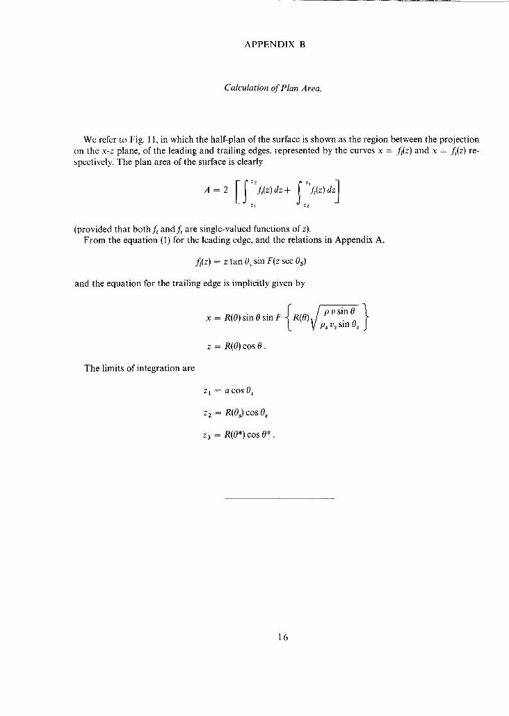
on the high pressure side. Owing to the strongly non-linear nature of the flow field the only feasible design method giving a configuration with exactly predictable properties appears to lie in the use of basic simple known flow fields, making use of the fact that stream surfaces can be replaced by solid surfaces. An example of this procedure is given by the 'Nonweiler wing '1'2 where the basic flow field is taken as that past a two-dimensional wedge and contains a plane oblique shock wave. The leading edge of the configuration is prescribed as a curve drawn on the shock wave and the lower surface of the configuration is obtained by replacing the stream surface through the leading edge by a solid surface. Thus the lower surface is designed to have a prescribed (constant) pressure coefficient. Examples are illustrated in Fig. 1. In Fig. la the 'curve' on the leading edge is prescribed as an 'inverted V'. The upper surface of the configuration has been taken as parallel to the free stream for simplicity. In practice any upper surface can be used that does not detach the shock wave from the swept leading edges. In Fig. lb it is shown how two simple flow fields can be combined to give a more general configuration.

The purpose of the present Report is to illustrate the possibility of using the flow field behind an axisymmetrical conical shock wave as the basic flow field, thus providing a wider selection of possible shapes for which the exact flow field is known. The leading-edge curve is now drawn on the conical shock wave, and the lower surface of the configuration is obtained, as before, by replacing the stream surface through the leading edge by a solid surface. The pressure coefficient on the lower surface is no longer exactly constant but (fortunately, since it is intended to design for prescribed conditions) the variation is not large. The extremes of pressure coefficient occur just behind the shock and on the cone, and these limiting values are plotted, for the case M = 4, as functions of cone semi-angle in Fig. 2. The effect of the adverse pressure gradient on the configuration boundary layer is an aspect of the method to be investigated experimentally.

Two basic types of configuration have been considered, depending upon whether or not the cone apex lies on the prescribed leading edge. The case where the cone apex becomes the apex of the configura~;,m is called a Type A configuration. In the Type B configuration the apex lies off the cone axis.

The principal difference between the Type A and Type.B configurations described is that in the former case wings and body are distinguishable as separate entities on the lower surface (the body being part of the basic cone) whereas in the latter they have been 'integrated'. Of course, by taking the apex of the configuration near to the cone apex a smooth transition between the two types can be obtained.

The overall forces due to the pressure on the lower surface might be computed by integrating the pressure over the surface. However, in Section 6 we have used momentum-integral methods to derive formulae for these forces, and by exploiting the conical similarity of the basic flow have reduced the expressions for lift, drag and pitching moment to single rather than double integrals.

It should be pointed out that the idea of replacing stream surfaces in the flow field past a non-lifting cone by solid surfaces has been used previously 3 in the design of precompression bump surfaces for use with supersonic inlets. The 'bump' generated in this case follows the stream surface defined by the curve of intersection of a conical shock wave and a plane parallel to the free stream.

2. Streamline Equations and Construction of Compression Surface. In axisymmetric flow a streamline through any point is wholly contained in the plane defined by that

point and the axis of symmetry. This means that in spherical polar co-ordinates r, O. rh (see Fig. 3) one of the equations defining a streamline is

t h = constant. (1)

The other equation can be derived from the continuity equation,

(~ (r2 sin Opu) + ~--~ (r sin Opv) = O, (2)

which is satisfied by some stream function g~ such that

~/i,3 ~v- = r 2 sin Opu O0

0-r- = - t" sin Opv.

In conical flow the dependent variables p, u and v are functions of 0 only. We therefore put

when

= r2f(0) (3)

1 df pu = sin 0 dO (4)

and

2 pv = sin 0 f(O)' (5)

The equat ions for a streamline,

= constant

~k = cons tan t ,

now become

~b = constant

r 2 p (0)v (0) sin 0 = constant t (6)

r z p(O)v (0) sin 0 = R 2 p(Os)V (Os) sin 02

= R z p, vs sin 0,, say,

= F(R)

(63 }

(using (5)).

Suppose that the leading edge of the lifting surface is given by

dp = F(r)

0 = Os ~ (7)

where 02 is the semi-angle of the basic conical shock. The equations for the streamline which intersects the leading edge at r = R are then

and the required lifting surface is the surface generated by all such lines for values of R from the apex to the intersection of the leading and trailing edges. By eliminating R from (6'), we obtain the equation for this surface:

/p(O)v (0) sin 0 "~ r j r Z(r, 0,~b) = (~-F l V psvssinO~ O. (8)

The intersection of the lifting surface with a plane normal to the axis of the basic cone, say the plane r = r 0 sec 0, is obtained by substituting for r. This yields

~b = F r osec0 Psv~sin()~ "

The actual shape of the lifting surface at that section is obtained by plotting 2 = r o tan 0 against ~b (see Fig. 4). The M.I.T. Cone Tables 4 contain all the data necessary for computing the argument of F in (8)

directly.

3. Type A Configuration.

3.1. General Properties.

We describe the sort of lifting surface formed when the leading edge extends to the apex of the basic conical shock as a Type A configuration. In this case, the leading edge might be described by the relations

0 = 0s L

¢ r(r) = +[¢o@(r)]

(7a)

where 6~(O) = 0. The Type A configuration permits a distinction to be made between the 'wing' (formed by the streamlines originating from the leading edge) and the 'body' (formed by part of the circular cone which supports the basic shock). We now deduce some of the properties of the intersection of the 'wing'

and the 'body'.

The problem reduces in essence to an investigation of how the derivative dO of the curve defined by

(9) behaves as 0 ~ 0<. From (9) (see Fig. 4) we have immediately that

/ d~b dF dR sin 0 P /) - whereR = r sec0 , / dO dR" dO ' V p~ v~ sin 0~"

Now> as 0 -~ 0c,

[ dR I [ p v sin 0

- [ s e c 0 t a n 0 / - . . . . ~-~ ro V psvssin°s

d } (p v sin 0)

+ sec 0 2-~/ps p vs v sin 0s sin 0

tends to infinity like (0-0c) -~, since v ( 0 ) ~ - 2 uc (0-0c), and

d (pv sin 0) = - 2 pu sin 0 --, - 2 Pc uc sin 0c.

Thus three cases can be distinguished :

(i) If dF de remains finite as 0 ~ Oc, when R -~ 0 like (0 - Oc) ~, then ~ tends to infinity like (0 - Oc)- +. The

'wing' is then tangential to the 'body' at 0 = 0 c; i.e. the two are smoothly faired together. I- dF d~)

(ii) f~--~ = O(R) = 0(0-Oc) "~, then )--ff has some finite value as 0 ~ 0c and the 'wing' intersects the

'body' at some angle between 0 and n/2 which will depend on the distance from the apex. ,tO

(iii) If dFdR = o(R) = o(0-0c) ~, then d0- tends to zero as 0 tends to 0c, and the 'wing" intersects the 'body'

at right angles.

3.2. Example of Type A Configuration. An example of a Type A configuration is illustrated in Fig. 5. The basic flow field is taken to be that

past a 10 ° semi-angle cone at M = 4. The upper surface has been constructed by taking generators parallel to the free stream through the leading edge whose front projection is an arc of a circle. The lower surface Cr. and L/Dp values thus become overall values for the configuration. Since the front projection of the leading edge has non-zero curvature at the apex, it follows from Section 3.1 that the trailing edge is tangential to the cone at the wing root.

Section AA (Fig. 5) illustrates the limiting form that all Type A configurations take near the apex. In particular it can be seen that the wing thickness tends to zero. In practice thickness can be obtained by adding a small amount of volume on the upper surface, the only necessary condition being that the re- suiting compression on the upper surface is not large enough to cause shock detachment. When the upper surface is parallel to the free stream the lower surface force data give overall values : CL = 0"075, L/Dp = 8.1.

4. Type B Configuration.

4.1. General Properties. We denote by the term 'Type B configuration' a lifting surface the apex of which lies behind the apex

of the basic cone. In this case, the surface does not include any part of the circular cone which supports the conical shock (i.e. 0 is always > 0c) and the distinction between 'wing' and 'body ' cannot be made. The leading edge could be given by

0 -~- 0 s

c~ = F(r) = +_ (r - a)" ~k ( r - a) (7b)

defined only for r > a. n is a number > 0, and ~k()0 a regular function of Z, such that ~b (0) :# 0. The apex of the lifting surface so formed is at r = a, and the 'ridge line' of this surface, that is, the trajectory of the streamline through the apex, is given by

~ p p~ v~ sin O~ r = a (0) v (0) sin 0

~ = 0 (lO)

do5 The 'ridge angle' (see Fig. 4) is determined by the behaviour of : ~ on the surface near that line, i.e. as

4' --* 0. In fact, if the intersection of the lifting surface and the plane r = r o sec 0 form a curve defined on that plane variously as

A (o, 4,) = (,l, 4,) = .t; (x, y) = o

(where 2 = r0 tan 0, and x and y are cartesian co-ordinates, as shown on Fig. 4), then the semi-ridge angle/~ is given by

/ ? = ~ - t a n - dyy f 3 : o , o : o

1( do,) = ~ - t a n - s i n 0 c o s 0 ~ ~

= 0 , 0 = 0 (11)

From (9), we have that

fl =4'-F f r°secOv/ pVsinO t

and on substituting for F from (7b), we find

d f l" f pvsinO a)/" (rosec v/pvsin° a)~ __do' / = l r 0 sec 0 , / - . . . . _ ~ 0 / I , = o +-~ \ V psvssinO~ dO ps v~ sin 0~

0 / o v sin 0 The limit 4, ~ 0 is equivalent to letting r o cos ~//;~ v~ sin 0~ --' a.

. a o , / Clearly, for 0 < n < 1, this passage to the limit results m ~ tending to infinity, giving /? = 0;

f~ =0 the ridge angle is then zero, and the section of the lifting surface is cusped. For n = 1, a ridge angle between

do, will tend to zero, giving/~ = hi2 and the 0 and n will in general be obtained, while for n > 1, ~/~ I,=o

ridge angle = n, i.e. the section of the lifting surface is smooth.

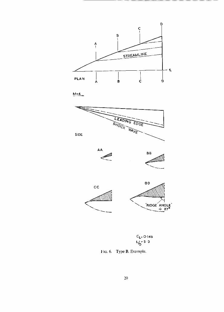
4.2. Example of Type B Configuration. An example of a Type B configuration is illustrated in Fig. 6. The upper surface comprises two inter-

secting planes with their line of intersection at an angle of attack. The upper surface intersects the conical shock wave associated with a 15 ° semi-angle cone at M = 4, and the leading edge is defined as the curve of intersection. The lower surface of the configuration is then obtained by replacing the stream surface through the leading edge in the cone flow field by a solid surface. The angle of attack of the upper surface was chosen by trial and error in order to give structurally reasonable wing tip angles in cross section. The resulting shape is a geometrically slender wing (aspect ratio approximately 1.6) with a fairly flat lower surface. This type of wing tends to a 'Nonweiler wing' at the apex. Integration of the pressure coefficient over the planform and front projections of the wing gives the lower surface data: CL = 0.146, L/Dp = 5"3. Owing to the sharp apex there is a ridge on the centreline of the lower surface (as in 'Non- weiler wings'). The magnitude of the ridge decreases from the 'Nonweiler' value at the apex as distance from the apex increases, as shown (Fig. 6).

5. Inverse Construction.

The methods developed above permit a simple inverse construction for a lifting surface, i.e. a con- struction of the leading edge from a given section at some plane r = r o sec 0. Suppose the section is given a s

0 = ® (~b) (or, equivalently, 2 = r0 tan 0 = A (~b))

in the plane. Then the leading edge is given by

R = r o sec ® (~b) •/p(_• v(O) sin ®

v~ sin O~

0 = Os (12)

The construction of some intermediate section, say at r = r 1 sec O, where rl < r o, must be done graphically, or by interpolation. The relationship between 0 and q~ at this section is implicitly given by

F1 (0) = - s e e 20v (0)p(O) sin 0

= F2 (~b) = - sec 2 O v(®) p(®) sin ®. (i3)

It should be remarked here that an inverse construction in which a Type B trailing-edge shape and an undisturbed flow Mach number are given is not unique. We have in this case the choice of a continuous range of shock wave angle 0~, from the maximum possible at that Mach number to the Mach angle; and for each 0s we may position our prescribed trailing-edge shape anywhere in the flow field provided only that its tips fall on the shock-wave surface, and it nowhere touches the conical body corresponding to the shock angle.

To obtain a unique surface it is necessary in this case to specify both 0~ and to.

Illustrative example. To illustrate the inverse method the shape of the leading edge, and of the section of the lower surface

at half-chord, were determined for a compression surface having a straight-line trailing edge in a certain conical flow. Details of this flow are as follows:

Moo = 4.07

0shock = 17 .520 (0cone = 10°);

and the trailing edge, at a section r = sec 0 in arbitrary units, is given by

tan 0 cos ~b = tan 13 °,

i.e. the trailing edge is a tangent to the circle 2 = tan 13 ° in the section plane. The plan of the lifting surface so derived is given in Fig. 7a, while in Fig. 7b the projections of the

leading edge, trailing edge, and section of lower surface at half-chord on the plane r = sec 0 (rear eleva- tions) are shown.

6. Formulae for Lift, Drag, and Pitchin9 Moment. The lift, drag and pitching moment on a surface E due to the forces of pressure on the lower side of

it are respectively

Z

M = f f ( P - P~o) i . (r x n) dS,

where n is the unit normal to Y,, directed away from the side on which the pressure acts, and in the ex- pression for M, r is the vector from the point about which the moment is to be taken to the element of area dS. Here and in what follows we employ, in addition to the spherical polar co-ordinate frame shown in Fig. 3, a related cartesian frame with co-ordinates x,y,z, associated unit vectors i, j, k, and velocity components vx, vy, and v z. The z-axis coincides with the line 0 - 0, and the plane x = 0 with the plane of symmetry of the compression surface. We list relations connecting quantities in the one frame with corresponding quantities in the other in Appendix A.

The direct evaluation of these integral expressions by graphical or numerical means is tedious, and in this section we reduce them to single integrals with respect to the variable 0.

We proceed from the general expressions for the steady flow of inviscid fluid, not experiencing any body force, through a fixed control volume:

pu. ndS = 0 (14)

f f~ f u(pu.n)+pn) dS = O (15)

I f (u×r)(pu.n)+p(nxr) dS=O. (16) s

Here the integration is over the surface S enclosing the control volume, n is the unit outward normal to the surface at any point on it, and r the position of the point relative to some origin.

In the trivial case when u -- 0, and p = constant = p~, the pressure of the undisturbed flo~v,

flp~ndS= ffP~(nxr)dS=O, J S $

whence (15) and (16) may be written

f f la(pu.n)+(p-p~)n} dS = O

ffJ(u×r)(pu.n)+(p-p~)(n×r)}dS=O.

(15')

(16')

Before specifying the control volume which we are to use, we shall provide for more general planforms than those treated up to this point, by supposing that the trailing edge be defined by the intersection of the compression surface with some surface of revolution r = R(0), or in the inverse case that the trailing

edge, defined in some other way, implicitly determines such a surface of revolution. The trailing edge is then the curve

r = R(0)

/ } (17)

The choice of trailing edge is restricted by the requirement that it be everywhere supersonic; if this were not so the conical similarity of the flow would be destroyed in some region.

We now apply equations (14), (15') and (16') to the flow in a volume enclosed by a surface made up of: (i) The compression surface E. (ii) The surface S 1, being that part of the surface of revolution given by r = R(O) which is enclosed by

the trailing edge and the intersection with the shock. (iii) The surface Sz + $3, where $2 is the normal projection of $1 onto the plane at right angles to the

undisturbed flow direction which passes through the apex of the surface Z, and S 3 is the normal projection of Y~ onto the same surface.

(iv) The cylindrical surface $4 formed by the sheet of undisturbed streamlines which, by the definition of $2 and $3 above, must connect the boundary ofSz + Sa with the upper boundary of E (the leading edge) and the lower boundary of S t (the circular arc formed by the intersection of the shock surface, 0 = 0s and the surface of revolution r = R(O)).

The control volume is illustrated in Fig. 8, which in the interests of simplicity shows the case for a compression surface with a trailing edge straight in plan, when the surface of revolution r = R(O) (= ro sec 0) is the plane z = r 0.

(a) Lift and drag. For the control volume described, we note that on $2+S~, p-p, = 0, u = k q , and n = - k ; on

Eu.n = 0 (since Z is a stream surface); and on $4 both u. n = 0 and p-p~ = 0. (since $4 is a stream surface in the undisturbed flow). Equations (14) and (15') then become respectively

-P~oq~o(S2+S3)+ f l P u.nds=O (18) 1

and

-p~q2 (Sz+Sa)k+ ffz(p-p~o)ndS+ ffs{u(pu.n)+(p-p~)n}dS=O (19)

The second term on the L.H.S. of (19) is simply D k - L j , where D is the drag and L the lift, and using (18), we absorb the first term into the third, to get

D k - L j + ff~ {(u-qook)(pu.n)+(p-po~)n}dS = 0 1

(20)

or, scalar-multiplying by j and k respectively,

L= ~f {u.j(pu.n)+(p-pJn.j}dS 1

D = - f~ {(u.k-q~)(pu.n)+(p-p~o)n.k} dS 1

(21)

(22)

We choose dS to be that element of the surface $1 (given by r - R(O) = 0) bounded by its interesections with the surfaces

0 = 0', 0 = O'+dO'

4~ = 4 ' , 4, = 4 , ' + d ¢ ' .

Then from consideration of the sketch of the element dS in Fig. 9, and using the relations listed in the Appendix, we have that

dS = R x/R 2 q- R '2 sin 0' dO' d~'

where

Re l -- R'e 2 n = ~ R , d

R = R(O') , dR(O')

R ~ - - dO'

and

L = f f R sin 0' cos ~b' {p(0') (u(O') sin 0 '+ v(O') cos 0') (u(O') R - v(0') R') $1

D =

+(P(O')-poo) (R sin 0 ' - R' cos 0')} dO' d~'

f f R sin 0' {p(0')(u(O')cos O'-v(O')sin O'-qo~) (u(O')R-v(O')R') t

+(p(O')-p~) (R cos 0 ' - R' sin 0')} dO' dc~'.

Both these expressions may be integrated with respect to ~6' immediately. The limits of integration are d e t e r m i n e d by e q u a t i o n (17), for the t r a i l i ng edge ; by s y m m e t r y 4~ goes f rom

f /p(O')v(O')sinO'} ~ 1/ ' } - F ~R(O')V p ~ v ~ n ~ t o + F R(O') p(O')v(O')sinO' L I / Ps vs s{n 0s . We now also suppress the primes on

variables of integration, and the expressions for lift and drag finally become :

On

f ({ g = 2 R s i n 0 s i n 1 R Vp~,;.,SinGj J x 0*

(23) x {p(u sin 0 + v cos 0) (uR - vR') + (p - Poo) (R sin 0 - R' cos 0)} dO

Os

D = - 2 R s i n 0 F R V p ,v~sinO~ x

x {p(u cos 0 - v sin O- q~) (uR - vR') + (p - p~) (R cos 0 + R' sin 0)} dO. (24)

10

Here the lower limit of integration 0* is the value of 0 for which equation (17) gives ~b = 0; it corresponds to the midpoint of the trailing edge.

(b) Pitchin9 moment. To calculate the pitching moment of the surface, we now use equation (16'). The vector r in it may

be taken from any fixed origin ; for concreteness we shall take the moment about a line through the apex of the wing parallel to the x-axis. We shall in what follows use the symbol r to denote the vector xi + yj + zk, and substitute for r in (16') the vector r' = r - a = x i + ( y - a sin Os)j+(z-a cos Os) k. Here a is the value of the co-ordinate r which in equation (8) gives q~ -- 0; in other words, the position of the apex of the surface is, in spherical co-ordinates (a, Os, 0), and is the origin for r'. With this substitution, we take the i - component of (16'):

-P~oq~ ff i . ( k x ( r - a ) ) d S + If (p-po~),.(nx(r-a))dS $2+$3 E

+ f i . {u x i f - a ) ( p u , n ) + ( p - p ~ ) n. i f - a ) } dS = 0

S1

(25)

The second term in this equation is the pitching moment about the apex, M, where M is reckoned positive in the nose-up direction. The first term in (25) (say, I~) reduces to

Ii = - p ~ q 2 asinOs(S2+Sa)+p~q 2 f f ydS.

$2 +$3

The integral in (26) is the moment of inertia of the surface S 2 -I- S 3 about the line given by

z = a cos 0 2

(26)

y = 0

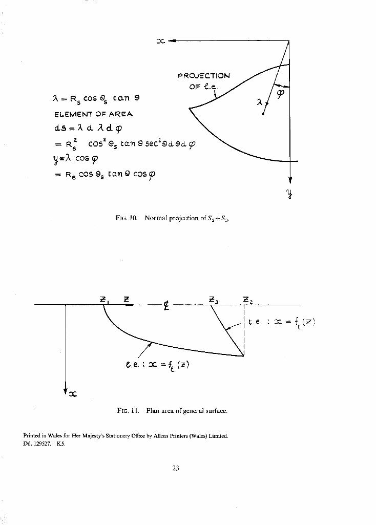
It is more convenient to evaluate this integral by projecting the surface normally to itself onto the plane defined by the intersection of the surface r = R(O) with the shock surface, 0 = 0~, i.e. onto the plane z = R(O~) cos 0s. This projection is shown on Fig. 10. The lower boundary of $2 + $3, is given by 0 = 0., in this plane, and the upper boundary, the normal projection of the leading edge onto the plane, by

t a n 0 "~ (a = + F R(Os) tan O~ ] .

The integral then becomes

f y dS =

82+83

f R a cos 3 02 tan 2 0 sec 2 0 COS ~ dO dO

S2 + Sa

f0 { Rtan0 } = 2 R ~ c o s a0s tan 20sec 20sin F \ S t an0s j dO.

11

We now turn to the reduction of the third term in (25) (say, -/3). ib is may be expressed as

/3 = ff{i.(uxr)(pu.n)+(p-p~)i.(nxr)IdS Sl

-(acosOsj-asinOsk). f f {u(pu.n)+(p-p~)n}dS. (27)

The second term in the expression for 13 is

- a cos 0~ L - a sin 0~ D + a sin O~ q~ f f pu. ndS, Sx

and we observe that, f rom (18)~ the last term in this cancels on addit ion with the first term for 11 in (26). Further , it can be shown that on the surface S1

i . ( u x r ) = Rcos~bv

and

i . (n x r) - R R' cos ~b

from which finally we may write the expression for M :

f °, { i f t a n 0 ) } M = + p~ 02 2 R 2 cos 3 0, tan 2 0 sec 2 0 sin " ~ R, i-ai~-o, dO

- a sin 0~ D - a cos 0~ L

Os

+2 ;oR2SinOsin(F (R~/pvsinO ~ dO.

(28t

Clearly, if for a sin 0~ and a cos 0~ in (28) we substitute the co-ordinates y = K z = Z of any point in the plane x = 0, then (28) will give the pitching momen t of the surface 2; about that point. Conversely, if M is set equal to zero, and y and z substi tuted for a sin 0s and a cos 0~, (28) yields the equat ion for the tr im line of the surface.

In reducing the values of L, D and M to the corresponding non-dimens ional coefficients Ct, Co, and ('M, a reference area characteristic of the surface is needed. In Appendix B, the calculation of the area

of the plan project ion of 2; is sketched.

Illustrative calculation. As an example of the use of the formulae developed above, the lift, drag, and pitching momen t abou t

the apex have been calculated for the surface which served as the illustrative example for the construct ion given in Section 5. (The shape of this surface in plan is shown in Fig. 7a).

12

The following results were obtained

CL = 0.0635

CD = 0.0055

C M = 0"0408.

} hence L / D = 11.6

In these results C L and C D were reduced with respect to the area of the surface in plan, and CM with respect to this area times the centre-chord of the surface in plan.

7. D i s c u s s i o n .

It has been shown how the flow field past a non-lifting circular cone at high supersonic speeds can be used to design the lower surface of a lifting configuration. The leading edge of the configuration is defined by means of a curve on the conical shock wave and the lower surface is obtained by replacing the stream surface through this leading edge by a solid surface. The configuration then supports a conical shock wave attached at its leading edges. The method is a direct extension of the method of Nonweiler 1'2 in which the flow field behind a plane oblique shock wave is utilised.

Examples of 'Nonweiler wings' are illustrated in Fig. 1, and three illustrations of the present method are given in Figs. 5, 6 and 7. By extending Nonweiler's design method to include configurations supporting conical shock waves a larger choice of shapes associated with exactly known flow fields is possible.

Two types of configuration, referred to as Type A and Type B configurations, depending upon whether or not the apex of the basic cone lies on the leading edge, have been illustrated. In the former case (Fig. 5) the wing and body are distinct, the body being part of the basic cone. The concentration of volume in the centre of these configurations is probably theirmost useful distinctive feature. In the latter case (Type B, Fig. 6) an 'integrated' configuration results. The possibility of providing a nearly flat undersurface with a flow field known in depth below it is useful in connection with the design of engine intakes.

Analogous work on the design of upper surfaces using axisymmetric expansion flow fields has been presented by Moore s. The methods can be combined to give a design method for complete configurations for flight at high supersonic speeds.

13

LIST OF SYMBOLS

CL

CD

CM

r,O,c~

hi, t~ W

x, y, z

Ux, 13y~ ~)z

P

P

()~

Lift coefficient

Drag coefficient

Moment coefficient

Spherical polar co-ordinates

Corresponding velocity components

Cartesian co-ordinates

Corresponding velocity components

Pressure

Density

Stream function

Quantity at shock wave

No. Author(s)

l T.R. F, Nonweiler ..

2 T . R . F . Nonweiler ..

3 R.E. Bower, R. S. Davies and R. E. Dowd ..

4 Z. Kopal . . . .

5 K.C. Moore . . . .

REFERENCES

Title, etc.

•. Aerodynamic problems of manned space vehicles• J.R. Aero. Soc. Vol. 63, pp. 521-528. 1959.

• • Delta wings of shapes amenable to exact shock wave theory.

J.R. Aero. Soc. Vol. 67, pp. 39--40. 1963.

•. Design and development ofprecompression bump surfaces for use .. with supersonic inlets.

Grumman Aircraft Eng. Corp. Rep. RE-122, 1959.

•. Tables of supersonic flow around cones. M.I.T. Dept. of Elec. Eng. Center of Analysis, Technical Report

No. 1. 1947.

•. The application of known flow fields to the design of wings with lifting upper surfaces at high supersonic speeds. A.R.C. 26913. R.A.E. Technical Report 65034. Feb. 1965.

14

A P P E N D I X A

Relations Connecting the Two Co-ordinate Frames.

whence,

x = r sin 0 sin ~b

y = r sin 0 cos ~b

z = r cos 0.

r = x / x 2 + y 2 + z 2

0 = tan -1 {(x2+y2)~/z}

0 = t a n - 1 (x/y).

i = sin 0 sin 0el + cos 0 sin ~be2 + cos 4~ e3

j = sin 0 cos ~bel + c o s 0 cos ~be2- sin ~be3

k = cos 0e~ - s i n 0e2.

(A.1)

(A.2)

(A.3)

el = sin 0 sin ~bi+ sin 0 cos ~bj+cos Ok

e 2 = cos 0 sin ~bi+ cos 0 cos q~j-s in Ok

e a = cos ~bi- sin q~] (A.4)

Relations connecting the velocity components in cartesian co-ordinates with those in spherical polar co-ordinates are obtained by substituting vx, vy, v~ for i, j, k, and u, v, w for el, e2, e3 in (A.3)andiA.4).

15

APPENDIX B

Calculation of Plan Area.

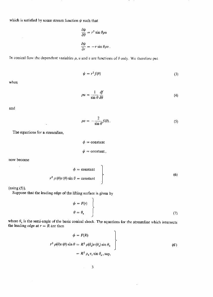
We refer to Fig. I l, in which the half-plan of the surface is shown as the region between the projection on the x-z plane, of the leading and trailing edges, represented by the curves x = f;(z) and x = fz(z) re- spectively. The plan area of the surface is clearly

A = 2 [ f~2 f t ( z )dz+ I ~(z)dz] Zl "-2

(provided that both f; andf~ are single-valued functions of z). From the equation (1) for the leading edge, and the relations in Appendix A,

fl(z) = z tan 0s sin F(z sec Os)

and the equation for the trailing edge is implicitly given by

The limits of integration are

( t x = R(O) sin 0 sin F R(O) V p s vs sin Os

z = R(O) cos O.

Z 1 = a c o s 0 s

z2 = R(Os) cos Os

z3 = R(O*) cos 0".

16

••sFT REE REAM

PLANE SHOCKS (a) (b)

FIG. 1. Nonweiler wings.

17

O-G

O ~ u

O'E

//

Cp

/

o ~o a o 3 o 4 o ~ (DEGKaES)

FIG. 2. Pressure coefficients in flow field past non-l if t ing cone at M = 4.

18

UaD

FIG. 3. C o - o r d i n a t e system, bas ic conical shock and body.

y~

H ~ B O D Y OCK

'~RIDGE ANGLE '/

E D

PLAN C

M = 4 5

I I I A 5 C D E

LEADING EDGE /

C L = 0 ' 0 7 5

L/Dp= 8" I

¢'-_ _

¢.

FIG. 4. Sect ion r = r o sec 0. FIG. 5. Type A. Example .

D C

/ J A B C D

M=4.=,

,,o~ ~.~'~----

AA

CC

S RIDGE ANGLE "~-....._..+__.87 °

FIG. 6.

CL= 0,146 L/D~ 5.3

Type B. Example.

20

1" FIG. 7a. Plan of wing with straight trailing edge.

J PI~OJECTION OF LEADIN G EE)~E (~.

S E C T I O N OF S U P P O R T E D SHOCK, A ' r T ~ I L I N ( ~ £Z)rqE

FIG. 7b. Rear view of wing with straight trailing edge.

21

i i / i ;~ i i

C . i - I ( " l ( ' l ~ ~ / ~ % 1 ~ " P--.I I I : D E A P ~

_L = .2,

S 2

E D G E

FIG. 8. Control volume.

0

E L E M E N T d.5

= R VR=+ R 'z sen O' d. O' d. ~'

NORMAL TO EL.S

-'y'°TC%,

FIG. 9. E l e m e n t o f a r e a o n r = R(O).

22

1° ROJ EC'I" I O1"4

= R s CO5 0 s Co.'rt ~ ~ , 9 , . #

EL.EMENT OF AREA.

d.5 : ;;', d. ,,,& cL cp

= R s COSmOs t&'n OSeC.zg&0c.L~

c o s

= R s COS 0 s I:;0.11 g COS

FIG. 10. Normal projection of S 2 + S a.

t . C . • £3C = ~C (2)

3C.

FIG. 11. Plan area of general surface.

Printed in Wales for Her Majesty's Stationery Office by Aliens Printers (Wales) Limited. Dd. 129527. K5.

23

]IRe & M[° Nee 3539

¢C) ()'own cop rrijzhl 1968

Published by } liar M AJEST;"S ~'l AJ IONhRY OI'FI( '1

To be put'chased frmn 49 [tJgh l lolborn, l_ondon w,( ,1 423 O~ford StreEt, l,ondoll w. 1 [ 1A Castle Street, Edinburgh 2

11)9 St Mary Street, ( 'ardlff ( ' I n I I JW Brazennose StrEet, ManchEstEr 2

50 Fail'fax ~treet, Bristol 1 IlSI ~l)k 258 259 Broad Street, Birmingham 1

7 I 1 Lmcnhall StreEt, Belfasl BT2 SAY or through any bookseller

R° & N[. No. 3539 S O Code N,, 2~-3539