the design, construction, and thermal diffusivity
TRANSCRIPT

Brigham Young UniversityBYU ScholarsArchive
All Theses and Dissertations
2018-12-01
The Design, Construction, and Thermal DiffusivityMeasurements of the Fluorescent ScanningThermal Microscope (FSTM)Samuel Hunter HaydenBrigham Young University
Follow this and additional works at: https://scholarsarchive.byu.edu/etd
Part of the Mechanical Engineering Commons
This Thesis is brought to you for free and open access by BYU ScholarsArchive. It has been accepted for inclusion in All Theses and Dissertations by anauthorized administrator of BYU ScholarsArchive. For more information, please contact [email protected], [email protected].
BYU ScholarsArchive CitationHayden, Samuel Hunter, "The Design, Construction, and Thermal Diffusivity Measurements of the Fluorescent Scanning ThermalMicroscope (FSTM)" (2018). All Theses and Dissertations. 7039.https://scholarsarchive.byu.edu/etd/7039

The Design, Construction, and Thermal Diffusivity Measurements of the
Fluorescent Scanning Thermal Microscope (FSTM)
Samuel Hunter Hayden
A thesis submitted to the faculty of Brigham Young University
in partial fulfillment of the requirements for the degree of
Master of Science
Troy R. Munro, Chair Matthew R. Jones Marc D. Killpack
Department of Mechanical Engineering
Brigham Young University
Copyright © 2018 Samuel Hunter Hayden
All Rights Reserved

ABSTRACT
The Design, Construction, and Thermal Diffusivity Measurements of the Fluorescent Scanning Thermal Microscope (FSTM)
Samuel Hunter Hayden
Department of Mechanical Engineering, BYU Master of Science
Over the life of nuclear fuel, inhomogeneous structures develop, negatively impacting thermal properties. New fuels are under development, but require more accurate knowledge of how the properties change to model performance and determine safe operational conditions. Measurement systems capable of small–scale, pointwise thermal property measurements and low cost are necessary to measure these properties and integrate into hot cells where electronics are likely to fail during fuel investigation. This project develops a cheaper, smaller, and easily replaceable Fluorescent Scanning Thermal Microscope (FSTM) using the blue laser and focusing circuitry from an Xbox HD-DVD player. The FSTM also incorporates novel fluorescent thermometry methods to determine thermal diffusivity. The FSTM requires minimal sample preparation, does not require access to both sides of the sample, and components can be easily swapped out if damaged, as is likely in irradiated hot cells. Using the optical head from the Xbox for sensing temperature changes, an infrared laser diode provides periodic heating to the sample, and the blue laser induces fluorescence in Rhodamine B deposited on the sample’s surface. Thermal properties are fit to modulated temperature models from the literature based on the phase delay response at different modulated heating frequencies. With the FSTM method, the thermal diffusivity of a 10 cent euro coin was found to be 21±5 mm2/s. This value is compared to Laser Flash Analysis and a Thermal Conductivity Microscope (which used thermoreflectance a method), which found the thermal diffusivity to be 30.4±0.1 mm2/s and 19±3 mm2/s, respectively. The hardware and instrumentation performed as expected, but the property measurements show that the device is not yet optimized to provide accurate measurements with current heat transfer models. Future work is discussed to investigate the accuracy and necessary modeling adjustments, as well as refinements to the instrumentation. Keywords: thermal diffusivity, fluorescent thermometry, photothermal, instrumentation

ACKNOWLEDGEMENTS
I would like to acknowledge the help of Dr. Troy Munro in teaching, mentoring, and
advising me throughout my time as a graduate student. I am very grateful for the time he took to
work with me and help me understand how to succeed. It was a challenging experience and Dr.
Munro helped inspire confidence in myself and prepare me for what comes next. I would also like
to acknowledge the incredible support of my wife, Eliza, who works extremely hard to help me
concentrate on and enjoy my work, and I hope that my efforts also support her to the same degree.
Our two kids, Elliot and Fiona, have also helped make life great. There are many other students
that have helped contribute to this research and process of making it through graduate school.
Ryker Haddock, Greg Bird, Spencer Diehl, Turner Palombo, Kegasi Turbovsky, and Sam Hales
have all contributed to the success and enjoyment of the project. Derek Sanchez and Peter
Hartvigsen, fellow TEMP lab students, have been great friends and associates to study and work
with, I would like to acknowledge the comradery that they have brought to the lab.
I would also like to acknowledge the funding from the Office of Graduate Studies to work
on this project and help undergraduates contribute to the project. The help of Zhourui Song, Zilong
Hua, and David Hurley is much appreciated to get the LFA and TCM measurements.

iv
TABLE OF CONTENTS
TABLE OF CONTENTS ............................................................................................................... iv
LIST OF TABLES ......................................................................................................................... vi
LIST OF FIGURES ...................................................................................................................... vii
1 Introduction ............................................................................................................................. 1
Motivation ........................................................................................................................ 1
Background ...................................................................................................................... 3
1.2.1 How Nuclear Fuel Changes Over Lifetime .............................................................. 3
1.2.2 Other Thermal Characterization Methods ................................................................ 5
1.2.3 Principles of Fluorescence ...................................................................................... 13
1.2.4 Fluorophores: Rhodamine B vs. Quantum Dots ..................................................... 14
Contributions of the Current Work to the State-of-the-Art ............................................ 16
2 Research Objectives .............................................................................................................. 20
3 Experimental Set-up and Methods ........................................................................................ 21
Laser Control Assembly and Troubleshooting............................................................... 22
3.1.1 Circuit Board Assembly and Troubleshooting ....................................................... 24
3.1.2 Focusing Photodiode Troubleshooting ................................................................... 25
Internal Photodiode ........................................................................................................ 26
Heating and Modulation Verification of Infrared Laser ................................................ 27
Focusing ......................................................................................................................... 30
Fluorescent Detection ..................................................................................................... 32
Lock-in Detection ........................................................................................................... 34
Motors and Sample Movement ...................................................................................... 35
4 Results and Discussion .......................................................................................................... 37
Euro Coin Data Collection ............................................................................................. 38
UO2 Data Collection....................................................................................................... 41
Error Analysis ................................................................................................................ 43
4.3.1 Potential errors from device design ........................................................................ 43
4.3.2 Statistical error analysis .......................................................................................... 44
Cost Assessment ............................................................................................................. 45
5 Conclusion ............................................................................................................................. 47
Limitations and Future Work ......................................................................................... 48
References ..................................................................................................................................... 51
v
Appendix ....................................................................................................................................... 55
Appendix A: Motor Datasheet used by HD DVD player and PHR Control Circuit Diagram .. 55
Appendix B: Modeling .............................................................................................................. 57
Introduction to Periodic Heat Absorption and Transfer ........................................................ 57
Heat Diffusion Model ............................................................................................................ 59
Appendix C: BOM .................................................................................................................... 66
Appendix D: Arduino Code ...................................................................................................... 67
Appendix E: How to Collect and Analyze Data ....................................................................... 80
Blu-ray Data Collection Process............................................................................................ 80
Curve Fitting Data with Fitmain.m........................................................................................ 81

vi
LIST OF TABLES
Table 1-1. Comparison of thermal property characterization methods ........................................ 18 Table 4-1: Comparison of values calculated with various methods, all in units of mm2/s. .......... 42 Table 4-2: T-test results for the euro coin. If the null hypothesis is not rejected, the results are
close enough between the systems that the difference can be attributed to only random error. .............................................................................................................................. 45

vii
LIST OF FIGURES
Figure 1-1: Stages of fuel material over its lifetime. With increasing time and temperature, the material changes as shown in [2]. ................................................................................... 5
Figure 1-2: Experimental set-up for laser flash. ............................................................................. 7 Figure 1-3: Heating method for STM methods............................................................................... 7 Figure 1-4: Schematic of metal film heating element (a). Possible shape for heating pads and
voltage sensing (b). ......................................................................................................... 8 Figure 1-5: Experimental set-up for FDTR. This schematic shows the pump and probe lasers,
optics for directing the lasers to the sample, and the photodiode and lock in for collecting and analyzing the signal. .............................................................................. 10
Figure 1-6: Method of scanning the probe laser to find the phase delay at a spatial distance from the pump heating spot, the phase delay increases in magnitude as the probe scans away from the center ..................................................................................................... 11
Figure 1-7: Heterodyne system experimental set-up. ................................................................... 12 Figure 1-8: Micro-photoluminescence spectroscopy experimental set-up. .................................. 13 Figure 1-9: Example of Stoke's Shift, where the emission peak is at a higher wavelength than
the absorption peak, shown by the arrows. This difference in wavelengths is different for each dye [1]. Image source: Wikipedia Commons, User: Zadelrob under a Creative Commons license. ........................................................................................... 14
Figure 1-10: Rhodamine B emission intensity over a 25 second heating period (left) and Quantum dot emission over the same period of time (right). The trend of decreasing intensity with increasing temperature is evident as the sample was heated by the laser. ....................................................................................................................................... 15
Figure 3-1: Block diagram of experimental set up. This diagram shows the components of the optical head, and the path of the fluorescent signal from the sample, to the photodiode, and then to the lock-in where it is compared to the reference and the phase delay ...... 21
Figure 3-2: Overview of laser control electronics. The commands are sent via Arduino (left), through the driver board (middle) then through the FFC cable to the PHR (right). ..... 22
Figure 3-3: Close up image of PHR laser assembly. Features of interest include the locations for multiple lasers, the dichroic for directing each laser down through the bottom of the assembly, and the built in focusing photodiode for focusing the laser ................... 23
Figure 3-4: PCB designed by Diyouware and built by hand after extensive troubleshooting. Solder bridges between the small pins shown in the magnified area on the FFC connector, was the most common issue stopping the focusing from working. ............. 24
Figure 3-5: Image of original Diyouware PCB (left) and customized PCB (right). The pads on the updated version are bigger and more consistent. .................................................... 25
Figure 3-6: Circuit board behind PHR focusing photodiode. These traces were used along with the photodiode datasheet (Melexis MLX75012) to determine which pins on the circuit board corresponded to the photodiode controls. ........................................................... 27
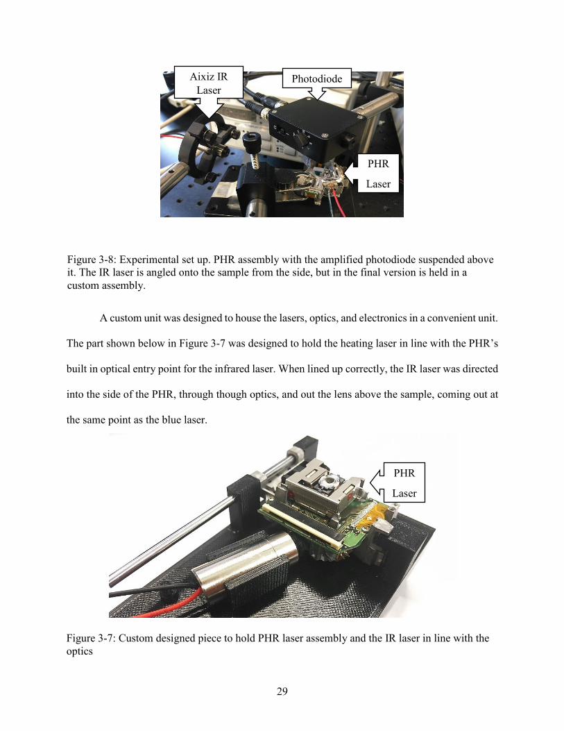
Figure 3-8: Custom designed piece to hold PHR laser assembly and the IR laser in line with the optics ............................................................................................................................. 29
Figure 3-7: Experimental set up. PHR assembly with the amplified photodiode suspended above it. The IR laser is angled onto the sample from the side, but in the final version is held in a custom assembly. .................................................................................................... 29

viii
Figure 3-9: Focusing states bases on the light reflected back onto the focusing diode. The left and right images result when the lens is too close or too far. The center is when the laser is in focus. ............................................................................................................. 30
Figure 3-10: Diagram of the S-curve generated by the internal focusing diode. The amplitude and focus region are denoted by a and a/16 respectively. ............................................. 31
Figure 3-11: Amplitude of the S-curve when focusing with the PHR's blue vs. focusing with the PHR's infrared laser ................................................................................................. 32
Figure 3-12: Image of coin with RhB deposited on surface. The color is different in certain areas due to the concentration of the dye regions. A and B show magnified images of the samples surface and how the distribution is uneven even at the mm scale, as well as the non-mirror like surface. ....................................................................................... 33
Figure 3-13: Graph of light intensity captured by a StellarNet Green-Wave spectrometer that measures between 350nm-1150nm. The peak at 405nm is the blue pump laser light, and the smaller peaks at 610nm are the fluorescent emission taken at four different locations on a sample. ................................................................................................... 34
Figure 3-14: Motor included in the Xbox assembly for moving the PHR laser assembly over a disc ................................................................................................................................ 36
Figure 3-15: Microscope images of calibration slide attached to motor to verify movement distance .......................................................................................................................... 36
Figure 3-16: Actual vs. Ideal motor location based on program input and measured location .... 36 Figure 5-1: Curve fit results for euro coin .................................................................................... 39 Figure 5-2: Image of sample with location of data points and resulting values overlaid. ............ 40 Figure 5-3: Curve fit on data collected with TCM on euro coin .................................................. 41 Figure 5-4: UO2 sample with RhB deposited on the surface ........................................................ 42 Figure A-1: Set up of system to be analyzed. The heating first hits the top layer of RhB particles
and is transmitted to the substrate. The model can account for two layers denoted by f for film and s for substrate .......................................................................................... 61
Figure A-2: Output of heat diffusion model using properties of Nordic gold, from 1 to 1000Hz 61

1
1 INTRODUCTION
Motivation
To help nuclear reactors be more accident tolerant, there is a need for thermal property
measurements of new materials, especially nuclear fuels. Nuclear fuel pellets are roughly 15
millimeters wide and can experience a temperature difference of hundreds of degrees Kelvin from
the center to the outer surface [3]. By the end of fuel’s life (high burn-up), non-homogeneous
microstructures form, causing hot spots and reducing heat transfer to the coolant. New accident
tolerant fuels are in development [4] that have improved thermal conductivity and thermal
diffusivity, but it is necessary to understand how their properties change over time to accurately
model their performance and determine safe operational conditions. More accurate models of the
thermal property distribution mean better predictive modeling. Understanding and predicting the
fission of radioactive elements and the effect of their distribution in the fuel helps prepare for
adequately cooling the fuel and keeping the reaction under control. If power generation becomes
uncontrolled, the reactor may become unstable and lead to the destruction of the containment
structure and release of harmful radiation to the surrounding area. Accidents in nuclear power
plants can have severe and long lasting consequences. Under accident conditions, heat
concentrations due to inhomogeneous material may cause the fuel rods to overheat unpredictably
[5]. Spent fuel with these heat concentrations can be analyzed to learn more about how the thermal
properties developed in the fuel. Current thermal property measurement systems are limited in

2
spatial resolution, cost, and do not integrate well into containment shelters shielded against
radiation, called hot cells (where electronics have a higher failure rate), for fuel investigation
during Post Irradiation Examination (PIE). The ultimate impact of this work is to attempt to
maintain nuclear safety with a much cheaper, smaller, and more easily replaceable device based
on the laser assembly from an Xbox to measure nuclear materials during PIE.
Thermal characterization, is important for predicting the behavior of materials in a variety
of applications. This project focuses on nuclear fuel, but other topics where knowledge of these
properties is important include combustion and energy generation. In these cases, the material
properties affect the efficiency, longevity, and safety of the process. In a gas turbine, engine
efficiency increases as the operating temperature goes up. Knowing the thermal properties of the
materials involved is key in improving these generation methods. When analyzing nuclear fuel
that experiences large temperature gradients over a small distance, the thermal conductivity at each
location determines the heat spread and distribution through the material. In such a complex
process it is important to know how the material will behave, understanding and predicting this
better can increase the safety of the process. The purpose of our sensor is to collect thermal
property data on nuclear fuel at various stages of use.
Current limitations of thermal conductivity measuring methods such as 3𝜔𝜔 [6], laser flash
[7], and laser reflectance [8] in determining the properties of these fuels include:
• High cost of replacing components damaged in a radioactive examination environment
• Inadequate spatial resolution
• Difficult sample preparation
• Incapability of measuring rough surfaces
• Low portability and large volume of equipment
3
• Difficulty of switching out damaged components remotely
• Cost of current sensors
Creating a measurement system that can overcome the bulleted limitations will make it
easier to analyze nuclear fuels and contribute to the data required to predict their behavior. To
address these difficulties, we propose to design, build, and test a sensor based on a commercially
available Blu-ray player to provide spatially resolved measurements of thermal properties. We will
make this thermal property instrument from a modified Blu-ray player to both sense and induce
temperature changes in the materials at a fraction of the cost of other thermal characterization
instruments. The motors in the Blu-ray player are also capable of the fine motor control required
to resolve these fine-scale properties. An inexpensive infrared laser diode (780nm) provides
periodic heating to the sample, and the blue laser in the Xbox optical head induces fluorescence in
fluorescent dye on the sample’s surface. A photodiode captures the emitted fluorescent light, and
a lock-in amplifier outputs the phase delay between heating and fluorescing for analysis in the
frequency domain heat diffusion equation to determine the thermal diffusivity of the sample.
Background
1.2.1 How Nuclear Fuel Changes Over Lifetime
Certain nuclear fuels, like U3Si2, show disagreements on experimentally collected data of
thermal properties [9]. One reason for this is the presence of significant impurity phases, requiring
more accurate analysis of how the thermal properties change over a range of temperatures and
manufacturing processes. It takes significant effort to analyze the data of these materials to get
sufficient data for capturing steady state operation conditions and design basis accident scenarios
[9]. There are many factors that contribute to changes in a fuel over its lifetime. Three of these
4
factors include fission product migration and swelling, pellet clad interaction, and restructuring
[2]. Restructuring is shown in the bottom left quadrant of Figure 1-1, along with the other
occurrences during the burn up lifetime. Fission products are atoms that appear in place of the
heavy-metal atom, and some of them become free to chemically attack the cladding material
around the fuel. Additionally, as the heavy-metal atoms are replaced, dimensional changes occur
as the fuel swells. Due to steep temperature gradients, these fission products can also migrate away
from the region where they are formed. Pressures of expanding gases may develop and the vapors
may also condense in cooler regions of the fuel element. Due to sharp temperature distributions,
the fuel pellet changes shape, causing it to interact with the cladding and increase stresses. The
fuel develops an hourglass shape due to a switch from plane-strain in the mid-plane to plane-stress
at the upper and lower faces. If the fuel is pressed against the cladding it can result in failure by
embrittlement or stress cracking. Pellet clad interaction (PCI) is a major source of cladding failure.
Restructuring of the fuel includes radial redistribution of component elements and substantial
swelling due to movement of insoluble fission gasses. This is also caused by the high temperatures
and gradients in the fuel. This restructuring results in the formation of a central hole Figure 1-1
columnar grains, and substantial grain growth just outside the columnar grain region. These
columns form along the direction of the thermal gradient. The temperature difference in oxide
fuels between the centerline and external surface can exceed 1000K over a small distance [2]. All
of these changes affect the thermal conductivity of the material. The thermal conductivity tends to
decreases, meaning heat does not leave the material as well and may result in hot spots [10]. This
project focuses on the work to characterize this local thermal conductivity degradation in other
samples in preparation for nuclear fuels.

5
1.2.2 Other Thermal Characterization Methods
There are many other methods for analyzing thermal properties of materials. Bulk property
measurements fall under the category of thermal parameter identification methods (a common
example of this is explained in the Laser Flash section below). Finer resolution measurements are
related to thermal topography. Topography indicates generating a map of the thermal properties at
each point of the sample’s surface, which is the proposed function of the FSTM. An overview of
these methods is presented here to understand the advancements that have been made in the field.
The methods reviewed include foundational techniques for bulk property measurement, time
domain methods, microscopic resolution, frequency domain methods, and methods that make use
of fluorescence in the temperature measurements.
Laser Flash A foundational work in property determination was by Parker et al [7], in which how light
pulses absorbed by a specimen can be analyzed at the opposite surface to determine the thermal
properties based on the delay between the temperature signals on either side of the sample. The
Figure 1-1: Stages of fuel material over its lifetime. With increasing time and temperature, the material changes as shown in [2].

6
samples analyzed with this method were coated with camphor black to maximize absorption and
ensure that the sample was heated uniformly. This method overcame difficulties of previous
methods when dealing with heater source and sink contact resistances. The sample was heated,
and the temperature rise on the opposite side was recorded via thermocouple. Recent versions of
this method use high speed IR sensors and improve modeling by considering subsurface light
absorption and radiation effects. This temperature response is modeled as the response to an
instantly absorbed pulse. Heat diffusion models for a thermally insulated and uniformly thick solid
relate the thermal diffusivity to the time it takes the heat pulse to heat the back surface of the
sample to half the maximum temperature rise. The resulting expression for thermal diffusivity is
𝛼𝛼 = �1.38𝐿𝐿2
𝜋𝜋2𝑡𝑡12
� (1)
where 𝐿𝐿 represents the thickness of the sample and 𝑡𝑡12 represents the time for the back surface to
meet half its maximum temperature rise. There are multiple assumptions in the LFA model,
pointed out in [11], and they also affect the experimental setup for this method, shown in Figure
1-2. The LFA model assumes one dimensional heat transfer, meaning the laser pulse width must
be sufficiently short to be considered negligible in comparison to characteristic time of the heat
diffusion process. Uniform heating is necessary on the front of the sample, and the sample must
be adiabatically insulated, homogeneous, and have a uniform geometry. The losses from the
surface are also neglected for the most basic models. This technique, combined with differential
scanning calorimetry and dilatometry, has been favored by the nuclear industry to measure the
thermal conductivity of fuels where 𝑘𝑘 = 𝛼𝛼/𝜌𝜌𝑐𝑐𝑝𝑝 [12], with 𝑘𝑘 representing the thermal conductivity,
𝛼𝛼 the thermal diffusivity, 𝑐𝑐𝑝𝑝 the specific heat, and 𝜌𝜌 represents the density. It is a proven method
for parameter identification of the bulk thermal diffusivity of a material. Other methods will be
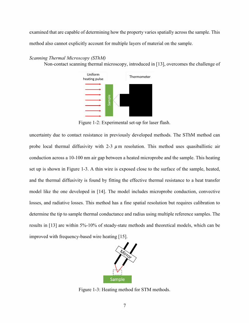
7
examined that are capable of determining how the property varies spatially across the sample. This
method also cannot explicitly account for multiple layers of material on the sample.
Scanning Thermal Microscopy (SThM) Non-contact scanning thermal microscopy, introduced in [13], overcomes the challenge of
uncertainty due to contact resistance in previously developed methods. The SThM method can
probe local thermal diffusivity with 2-3 𝜇𝜇m resolution. This method uses quasiballistic air
conduction across a 10-100 nm air gap between a heated microprobe and the sample. This heating
set up is shown in Figure 1-3. A thin wire is exposed close to the surface of the sample, heated,
and the thermal diffusivity is found by fitting the effective thermal resistance to a heat transfer
model like the one developed in [14]. The model includes microprobe conduction, convective
losses, and radiative losses. This method has a fine spatial resolution but requires calibration to
determine the tip to sample thermal conductance and radius using multiple reference samples. The
results in [13] are within 5%-10% of steady-state methods and theoretical models, which can be
improved with frequency-based wire heating [15].
Figure 1-2: Experimental set-up for laser flash.
Figure 1-3: Heating method for STM methods.

8
3ω Method The 3ω method is an AC technique (based on analysis in the frequency domain) of
measuring thermal properties [6, 7, 16, 17]. When first published, this method overcame common
problems due to sensitivity to black body radiation. This sensitivity was no longer a problem
because the samples were very thin compared to samples where sensitivity to black body radiation
had a larger effect [6]. The 3ω method involves applying a current controlled sinusoidal heating
of a metal layer deposited onto a surface (Figure 1-4) at 1ω and locking into the 3ω voltage
response. 1ω represents the frequency of the heating wave and 3ω is three times that frequency,
which corresponds to the desired response. In the 3 ω method, it is required to know 𝑑𝑑𝑑𝑑/𝑑𝑑𝑑𝑑, the
slope of the average resistance as a function of temperature, to determine 𝑘𝑘. The amplitude and
phase are measured over a range of frequencies [18]. Where time domain methods measure the
time to a certain temperature, this method analyzes the temperature responses in the frequency
domain.
Sample preparation can involve polishing the surface to a near mirror finish or ultrasonic
cleaning in acetone. This is then followed by lithographic deposition of the thin metallic heater.
This is because it is necessary to lay a pattern of pads for joule heating and voltage measurements.
This method is good for high temperature measurements done up to 750K [6], and compared to
others the time for equilibration is much shorter, just a couple oscillations of the heating element.
This method has been successfully applied to fresh nuclear fuels [19], but not irradiated samples
Figure 1-4: Schematic of metal film heating element (a). Possible shape for heating pads and voltage sensing (b).
9
because of the expected effect radiation damage will have on the metallic heater. Additional, the
ability to provide spatially resolved measurements is not possible.
Thermoreflectance Methods Thermoreflectance methods can be analyzed in the time or frequency domain [8, 20-22].
These methods involve a modulated heating (pump) laser to heat a sample and a sensing (probe)
laser reflected off the sample’s surface into an optical detector. The path of this light and the
electrical connections are shown in Figure 1-5. The surface of the sample is heated via laser, and
as the surface temperature changes, so does the reflectance. Reflected light that varies with
temperature is collected by a photodiode.
The Frequency Domain Thermoreflectance (FDTR) method [21] is another frequency
domain method that measures the changing reflectance, where the amplitude and phase lag are
measured in comparison to the heating signal. The properties can then be determined by fitting the
resulting data to the appropriate frequency domain model of the heat equation [11]. This method
uses a lock-in amplifier to collect the amplitude and phase response data of the reflected beam.
Because the phase delay also contains the delay due to cables and instruments, the work presented
in [21] splits a portion of the pump laser light to be sent to an identical photodetector and is used
as the reference for the lock-in amplifier. This reference signal is valid as long as the sum of the
path that the light travels is the same as that of the reflected probe beam detector. The time domain
version of thermoreflectance methods also use a pump and probe laser set up, but a transient
temperature change is measured, instead of the phase delay of a modulated signal. The time domain
method requires complex instrumentation, including high speed pulsed lasers and complex optical
table set-ups. This method is used at the Idaho National Laboratory with their Thermal
Conductivity Microscope (TCM) for property measurements [23]. One shortcoming of this method

10
is the necessity of a mirror like finish and adding a highly reflective material to the samples surface
to ensure adequate reflection of the probe laser. While this removes the surface structure of the
sample, it acts as a reference value to determine the thermal conductivity.
Thermal Conductivity Microscope (TCM) The Thermal Conductivity Microscope was invented an Idaho National Labs and is
designed to simultaneously measure local thermal diffusivity and conductivity [24]. The device
continuously heats a sample with a modulated laser beam, and the relates the temperature response
is related to a reflected optical signal (shown in Figure 1-6). Based on temperature induced changes
in reflectivity, the thermal properties can be inferred. The sample is coated with a thin layer of
gold to ensure strong optical absorption, and also establish a boundary condition that contains the
sample’s thermal conductivity. The data of interest is the phase lag of the reflected light of the
probe beam as its distance from the pump heating spot is changed. The phase lag increases as the
probe laser moves away from the location of heating, and the slope of the phase profile can be
related to the thermal properties.
Figure 1-5: Experimental set-up for FDTR. This schematic shows the pump and probe lasers, optics for directing the lasers to the sample, and the photodiode and lock in for collecting and analyzing the signal.

11
Heterodyne Picosecond Thermoreflectance The heterodyne picosecond thermoreflectance (HPTR) method eliminates errors and
artifacts in the signal to be analyzed, such as background noise and misalignment of pump and
probe beams. To fix these issues, this method uses two pump and probe lasers at slightly different
modulation frequencies. This frequency offset is shown in Figure 1-7 where the pump is modulated
at 76 MHz and the probe at 76.006 MHz. The heterodyning method is a way to extract data that is
represented in the modulated frequency of the signal. The particular method referenced was
developed for multi-layer samples. The modeling developed in [25] makes four major
assumptions. These include a pump duration that is much shorter than the scale of the experiment,
cylindrical symmetry of the temperature field, uniform temperature variation within the deposited
metal layer on the surface, and that the substrate is a semi-infinite medium. The use of multiple,
large Ti. Sapphire lasers, and the remaining optics are not easily integrated into a hot cell
environment.
Figure 1-6: Method of scanning the probe laser to find the phase delay at a spatial distance from the pump heating spot, the phase delay increases in magnitude as the probe scans away from the center

12
Micro-Photoluminescence Spectroscopy In reviewing the literature on non-contact measurements of thermal properties, one
particular source was mentioned in [11] to have used fluorescence. This method is presented in
[26] and presents measurements on individual nanowires with temperature dependent micro-
photoluminescence spectroscopy. This work sought to advance understanding of thermal transport
in low-dimensional materials. A 405nm laser was used to simultaneously heat and excite
fluorescence in the sample, shown in Figure 1-8. Spectra were captured at different temperatures
and the modeled heat conduction through a solid rod of given cross section was analyzed to
determine the thermal conductivity of the nanowires. Radiative heat loss was ignored because
when quantified at its peak, it was much smaller than the heat flow due to conduction through the
wire. This is relevant to this FSTM project because conduction is the main source of heat transfer
in the samples that each method measures. Other methods have used fluorescence to successfully
analyze spider silk thermal properties [27].
Figure 1-7: Heterodyne system experimental set-up.

13
1.2.3 Principles of Fluorescence
A novel aspect of the FSTM is the use of fluorescent thermometry. The following is a
general overview of fluorescence and its defining characteristics. When an electron is excited into
a higher energy state by a shorter wavelength (and hence higher energy) light, its return to the
ground-state orbital results in the emission of a photon. One characteristic of the fluorescent
process is that the emitted photon is at a longer wavelength than the exciting light because of
vibrational losses of the electron. This longer wavelength light can be related to temperature for
non-destructive thermometry measurements because of the relationship between increased
temperature and more vibrational energy losses [15]. This difference in wavelength between
absorption and emission is called the Stokes Shift, and is evident on absorption and emission
graphs for fluorescent dyes as seen in Figure 1-9.
Another interesting property of fluorescence is that the emission wavelength is independent
of the excitation wavelength, known as Kasha’s rule [28]. This is useful when a particular emission
wavelength is necessary, because any probe laser of higher energy could excite it, though there is
usually an excitation wavelength that will result in the highest quantum yield of emission. This is
apparent in Figure 1-9 where a peak in emission is evident.
Figure 1-8: Micro-photoluminescence spectroscopy experimental set-up.

14
These methods of relating the emission to temperature have been successfully used to
measure the thermal diffusivity of thin fibers and glycol [16]. Relating temperature in
measurements when heat input is by light fall under the broad umbrella of photothermal techniques.
1.2.4 Fluorophores: Rhodamine B vs. Quantum Dots
Two options for the fluorescent dye include Rhodamine B and quantum dots. Within the
group of inorganic fluorophores, quantum dots are of interest due to their stability and ease of
application to a surface. Quantum dots are inorganic nanocrystals with a variety of useful
applications. Due to their unique properties it is possible to synthesize particles with a tunable light
emission. Their photoluminescent properties mean that as they absorb photons of light, electrons
are excited to a higher state and a photon is emitted as the electron returns to its original state. By
adjusting the size of the quantum dots, which range from 2 – 10 nm, fluorescent emission can be
chosen between 400 and 4000 nm [29].
In addition to inorganic quantum dots as a fluorescent dye, there are organic dyes that
exhibit similar photoluminescent properties. One prominent example is Rhodamine B (RhB).
Rhodamines are a fluorophore, that when synthesized into a dye exhibit fluorescent emission with
Figure 1-9: Example of Stoke's Shift, where the emission peak is at a higher wavelength than the absorption peak, shown by the arrows. This difference in wavelengths is different for each dye [1]. Image source: Wikipedia Commons, User: Zadelrob under a Creative Commons license.
15
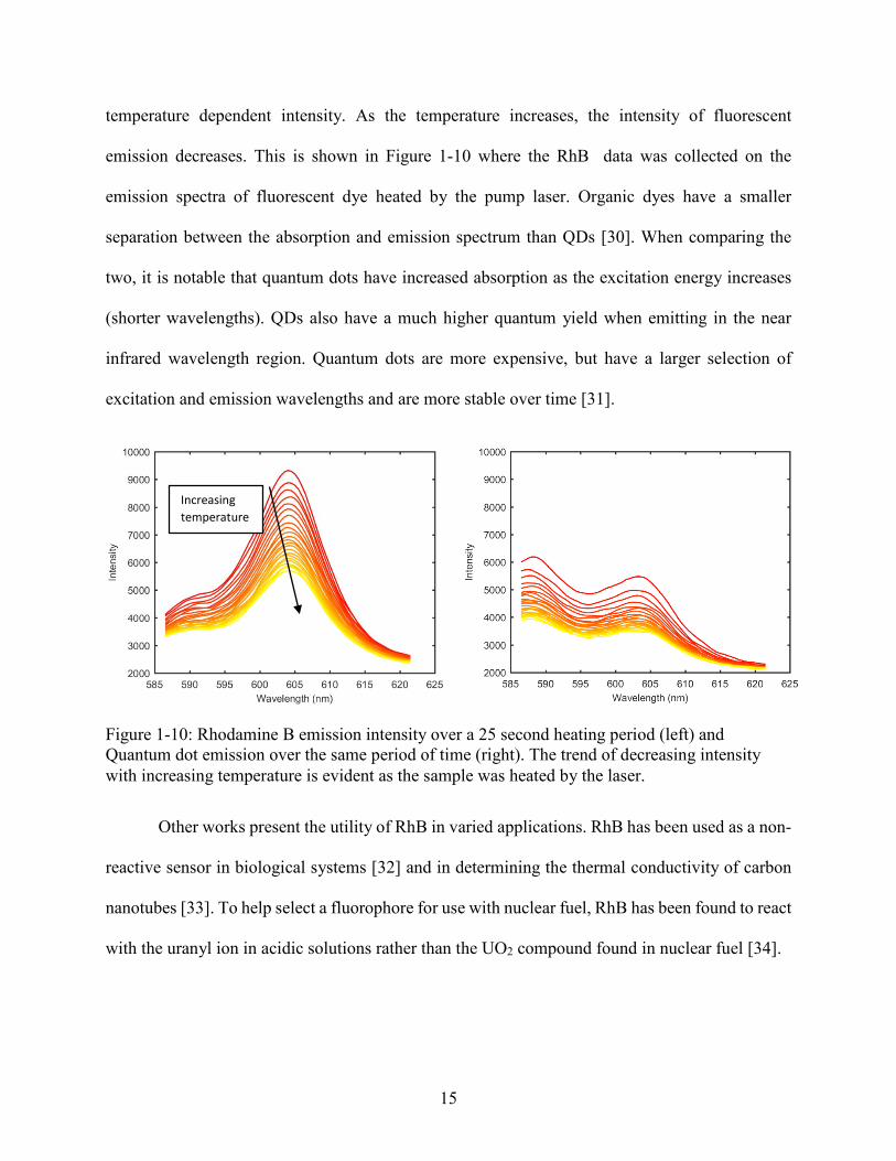
temperature dependent intensity. As the temperature increases, the intensity of fluorescent
emission decreases. This is shown in Figure 1-10 where the RhB data was collected on the
emission spectra of fluorescent dye heated by the pump laser. Organic dyes have a smaller
separation between the absorption and emission spectrum than QDs [30]. When comparing the
two, it is notable that quantum dots have increased absorption as the excitation energy increases
(shorter wavelengths). QDs also have a much higher quantum yield when emitting in the near
infrared wavelength region. Quantum dots are more expensive, but have a larger selection of
excitation and emission wavelengths and are more stable over time [31].
Other works present the utility of RhB in varied applications. RhB has been used as a non-
reactive sensor in biological systems [32] and in determining the thermal conductivity of carbon
nanotubes [33]. To help select a fluorophore for use with nuclear fuel, RhB has been found to react
with the uranyl ion in acidic solutions rather than the UO2 compound found in nuclear fuel [34].
Increasing temperature
Figure 1-10: Rhodamine B emission intensity over a 25 second heating period (left) and Quantum dot emission over the same period of time (right). The trend of decreasing intensity with increasing temperature is evident as the sample was heated by the laser.

16
Contributions of the Current Work to the State-of-the-Art
While the methods discussed in the previous section are dependable and well established,
laser flash is limited to finding bulk properties, while the other five are based on equipment that is
expensive, not suited for use in a highly radioactive environment that causes electronics failure
[35] and optical browning, or may require lengthy sample preparation procedures like polishing
the samples. This poses problems if the surface of the sample should be preserved. Additionally,
the other methods that employ the use of fluorescence have been performed on nanowires, spider
silk, and glycol, which have very different geometric and material properties than nuclear fuels.
The analysis of different geometries and properties will contribute to the variety of scenarios that
fluorescent photothermal methods have been tested and analyzed. Additionally, this method will
examine point wise properties, instead of bulk, which have not been examined in depth in other
fluorescent methods.
In addition to the methodology involved, this project contributes new instrumentation for
thermal property determination experiments that will advance the state-of-the-art methods. The
PHR-803t is an inexpensive laser assembly that comes out of an Xbox Blu-ray player. It contains
lasers, lenses and a focusing system and is readily available. This compact optical head reduces
the amount of engineering and cost of the FSTM. It contains the circuitry and components
necessary for focusing the laser, inducing fluorescence, and holding the heating laser, all in a
compact and easily replaceable unit. Its use was inspired by open source software and circuit
boards worked on by hobbyists and hackers. The most prominent example of controlling the
circuitry of the device was accomplished by [36] for the purpose of making a circuit board printer.
The methods of controlling the focusing fixture and laser diodes in the PHR are proprietary to
DVD player manufacturers, but the circuitry was reverse engineered and the circuit board in
Appendix A was developed to control the lasers and focusing built into the PHR. The focus of the
17
current project seeks to refine the optical control of the PHR-803t and contribute a useful
instrument to nuclear fuel and thermal property analysis. This project also contributes to more
affordable and simple nuclear fuel analysis. Because of the irradiated environment that these types
of measurements take place in that cause electronics to fail, device replacement can be costly.
Because the PHR-803t has many of the electronics self-contained, when device failure arises, the
optical head can be swapped out with minor cost consequences. This will make fuel analysis more
feasible by simplifying the process when parts fail and lowering the cost. This thesis is limited to
validate the performance of this device in measuring thermal diffusivity of a solid material. Future
work will use the device to understand how nuclear fuel will perform in a reactor. This specific
project is to use a working sensor to take data on materials of known thermal diffusivity measured
with standard techniques.
The FSTM device presented in this thesis uses fluorescent thermometry to measure
pointwise properties. This is a well-developed temperature sensing method for use with
thermometry techniques [30, 31, 37], and requires a dye, short wavelength laser, and photo-sensor.
To sense the temperature of a spent fuel or calibration sample, a fluorescent dye needs to be
deposited on the surface of the sample. This dye emits a specific spectrum of light that varies with
temperature when excited with the blue laser. Two options for the fluorescent dye include
Rhodamine B and quantum dots.
Like the FDTR method, this device involves a modulated pump laser to heat a sample, but
instead of a probe laser being reflected into an optical detector, the fluorescent dye is excited by a
probe laser for temperature variation detection by a photodiode. Similar to the frequency domain
methods discussed previously in literature review, the FSTM uses a lock-in amplifier to analyze
the modulated light data from the amplified photodiode. The FSTM also heats samples via infrared

18
laser. In laser flash analysis, the temperature changes are sensed by infrared camera, and in 3ω by
the heating pads. The FSTM method shares certain characteristics with some other methods, and
combines them into a unique system.
The information in Table 1-1 presents a comparison of the performance of laser flash,
thermal conductivity microscope (TCM), and a heterodyne laser system to the FSTM. At 1μm
optical resolution the fluorescent Blu-ray method is comparable to the TCM, finer than the 2-6μm
of the Heterodyne System. The laser flash resolution is not a relevant measure of comparison, as
it is used for bulk parameter identification and not mapping spatially varying properties. However,
because laser flash analysis (LFA) is the primary method of analyzing nuclear fuels, we include it
in some of our comparisons. The major advantage of the Blu-ray system is the size and cost. It is
under a thousand dollars while others range from $20-130k. Additionally the experimental set up
takes up less than half the volume of the next smallest set up, which is the LFA. These systems are
compared in Table 1-1.
Table 1-1. Comparison of thermal property characterization methods
This project seeks to advance the area of non-destructive thermal property measurements.
An overview of the field in [11] discusses many non-contact methods, with only one mention of
fluorescence in 200 references cited. These fluorescence methods have been limited to micro-
photoluminescence spectroscopy that analyzes nanowire. While fluorescent thermometry is well
LASER FLASH (LFA)
TCM HETERODYNE LASER SYSTEM
FSTM
SIZE 22 x 21 x 34 cm 56 x 20 x 25 cm ~100 x 50 x 25 cm 25 x 18 x 15 cm
COST
$100k+ $20-30k ~$130k <$10k
UNCERTAINTY ~5-10% [11] ~10% [11] ~10-15% [11] ~5-15% [38] previous fluorescent systems
RESOLUTION N/A Laser spot size 1 μm Thermal wave size ~50 μm
2-6 μm Laser spot size 0.6 μm

19
established in many applications, this project refines a novel use of fluorescent thermometry to
contribute to the field of non-destructive property measurements. The advantages of this include
simple sample preparation, non-destructive heating and data collection, requires access to only one
side of sample, preserves surface structure of sample to be analyzed, and low cost components for
temperature sensing. Another contribution of this project is the use of commercially available
optical heads as a device for scientific measurements.

20
2 RESEARCH OBJECTIVES
The objectives of this project can be broken up into the following main tasks. These are:
• Assemble circuitry to control PHR-803t lasers and focus them, and use it to develop a
modulated laser heating system.
• Collect fluorescent emission data emitted from sample’s surface with the FSTM.
• Determine suitability of PHR’s built in motors for use in moving the sample for pointwise
measurements
• Use appropriate mathematical models to extract the thermal diffusivity from the acquired
data.
• Determine the capability of the device to measure thermal properties samples of known
and unknown material composition and properties.
21
3 EXPERIMENTAL SET-UP AND METHODS
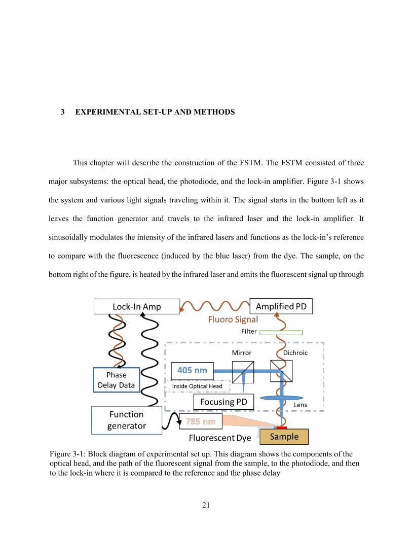
This chapter will describe the construction of the FSTM. The FSTM consisted of three
major subsystems: the optical head, the photodiode, and the lock-in amplifier. Figure 3-1 shows
the system and various light signals traveling within it. The signal starts in the bottom left as it
leaves the function generator and travels to the infrared laser and the lock-in amplifier. It
sinusoidally modulates the intensity of the infrared lasers and functions as the lock-in’s reference
to compare with the fluorescence (induced by the blue laser) from the dye. The sample, on the
bottom right of the figure, is heated by the infrared laser and emits the fluorescent signal up through
Figure 3-1: Block diagram of experimental set up. This diagram shows the components of the optical head, and the path of the fluorescent signal from the sample, to the photodiode, and then to the lock-in where it is compared to the reference and the phase delay

22
the PHR. The fluorescence is generated by the blue 405nm laser in the center of the figure that
travels from the diode and through mirrors and lenses down to the sample. The signal from the
sample and the other light travels up through optical filters and into the amplified photodiode. This
modulated signal leaves the photodiode and goes to the lock-in amplified where it is compared to
the reference, the phase delay is calculated, and sent to the computer via GPIO. The laser PHR is
controlled through a special driver board designed by Diyouware [36] that receives signals from
an Arduino MEGA coded to turn on the lasers, start the focusing algorithm, and process the
focusing signal coming back from the PHR. These three components are shown in Figure 3-2 and
discussed in detail in the following chapter sections. Arduino code is given in Appendix D.
Laser Control Assembly and Troubleshooting
A PHR-803t optical head was used as the laser assembly for the FSTM. The PHR-803t
laser assembly is from an Xbox 360 and it houses three laser diodes. The wavelengths of the laser
diodes are 405nm, 680nm, and 780nm. The benefits of this optical component include the low cost
(ease of replacement if damaged during use), tightly integrated optics, and focusing capability, the
components for these functions are pointed out in Figure 3-3. It is connected to the control circuitry
by a flex cable connected to the built in flexible flat cable (FFC) adapter, from which it can be
easily separated and replaced. Two lasers are necessary for the fluorescent thermometry, one to
Arduino MEGA
Figure 3-2: Overview of laser control electronics. The commands are sent via Arduino (left), through the driver board (middle) then through the FFC cable to the PHR (right).

23
heat the sample (pump) and one to induce fluorescence (probe) in a fluorescent dye deposited on
the sample.
Because the PHR-803t’s built in laser driver (ATMEL ATR0885) can only turn on only
one of the three lasers at a time, the blue laser is powered directly through the diode’s anode and
cathode using a constant current regulator that holds the current at ~85mA. A waveform generator
(Agilent 33220A) outputs a sinusoidal signal that varied the amplitude of the heating laser by
controlling the current through the diode. Because the IR laser in the PHR-803t was very low
power (~10 mW), it did not heat the surface enough to produce detectable temperature fluctuations
and an IR laser external to the PHR-803t was used. The data presented was collected with an
external heating laser (785nm, 90mW) directed at the sample, aligned concentrically with the
probe laser spot. Future devices will use a diode held in the position of the original diode by a 3D
printed assembly. The infrared laser spot was centered over the blue laser spot and kept at such a
distance that the infrared laser spot was larger than the blue so that the area of fluorescence was
evenly heated by the beam, to allow for the assumption of 1D heating.
Figure 3-3: Close up image of PHR laser assembly. Features of interest include the locations for multiple lasers, the dichroic for directing each laser down through the bottom of the assembly, and the built in focusing photodiode for focusing the laser

24
3.1.1 Circuit Board Assembly and Troubleshooting
The driver board designed by Diyouware [36] handles the signals that move between the
Arduino and PHR in either direction. From the Arduino the commands are sent to turn lasers on
or off and adjust their power. The driver board also processes a PWM signal from the Arduino to
move the focusing lens up and down. The PHR also sends the focusing signal from its photodiode
through the driver board where its components are combined, filtered and combined again before
being read by the Arduino. Assembling the driver board stenciling solder paste onto the circuit
board, placing the correct components according to Diyouware’s instructions, and reflow soldering
it in a reflow oven. The FFC connector, shown in Figure 3-4, often had solder bridges between
multiple pins after the reflow heating process, and it was necessary to remove them afterwards
with either a solder vacuum or solder wick. This problem was very difficult to overcome and the
circuitry was transferred to a breadboard, sacrificing compactness, but making it easier to build
the circuit section by section and solve problems as they arose. This made it possible to isolate
issues and build a functioning circuit.
Figure 3-4: PCB designed by Diyouware and built by hand after extensive troubleshooting. Solder bridges between the small pins shown in the magnified area on the FFC connector, was the most common issue stopping the focusing from working.
3.25mm

25
3.1.2 Focusing Photodiode Troubleshooting
Until the circuitry was transferred to the breadboard, the lasers were able to be turned on
and off, but the focusing did not work. Making more boards resulted in the same error and the
problem could not be found. The signal from the focusing photodiode could not be measured with
the oscilloscope and led to in depth troubleshooting to see where the focus error signal was being
lost. The focusing photodiode has four quadrants that collect reflected light, when two quadrants
are summed and subtracted from the other two the result equals zero when the laser is focused,
meaning equal amounts of light are hitting each segment. But this signal did not transfer through
the intermediate components and could not be measured at the output. One possible reason
frequently mentioned by the designers of the circuit was noise. To eliminate noise, the ground lines
between the digital and analog parts of the control circuit were isolated and grounded separately
with a shielded cable on the cable that carried the focusing signal from the laser assembly to the
Arduino in order to reduce the noise. The issue was eventually narrowed down to the small solder
connections on the FFC cable adapter where solder bridges were frequent and nearly impossible
to remove. On the boards where the solder bridges were removable the focusing worked, moving
it to a breadboard eliminated this issue. To address the issue and still be able to use the compact
PCB, the eagle source files were edited to increase the pad size for the FFC connector solder points.
As shown in Figure 3-5 on the right, the pads on the customized PCB are wider and more consistent.
Figure 3-5: Image of original Diyouware PCB (left) and customized PCB (right). The pads on the updated version are bigger and more consistent.
4.5mm

26
Internal Photodiode
To take advantage of the tightly integrated optics of the PHR laser assembly, the initial
plan was to use the focusing photodiode to focus the laser and also collect data on the intensity of
the sample’s emitted fluorescent light. Reading the documentation for the focusing photodiode
(Melexis MLX75012, Figure 3-6), the SW1 and SW2 were identified as the pins that changed the
sensitivity of the detector. These pins were located by disassembling one of the laser assembly
photodiode’s and tracing the pins (shown in the bottom middle of Figure 3-6) to the end of the flex
cable through the small electrical traces in the bottom middle image of Figure 3-6. The orientation
was verified by checking the pins that were already connected to the Diyouware driver board, it
was then necessary to identify the other ones. The data sheet was then used to trace each pin back
to its corresponding flex cable wire by following the PCB traces and vias shown in Figure 3-6 and
using a multimeter to check continuity between pins and flex cable connection points. Once traced
to the flex cable it was possible to probe them with an oscilloscope and measure the voltage
response to light input. With the pins identified, it was noted that they were receiving 4.2 volts,
meaning that the photodiode was already at maximum sensitivity, shown by the settings in the data
sheet segment of Figure 3-6. Examining the output of the focusing photodiode under multiple
conditions it was determined that the photodiode only outputs a signal when the laser focuses.
Otherwise the signal is constant and could not be related to light intensity, because of this we chose
a Thorlabs PDA36A amplified Si photodiode for fluorescent detection, while the internal
photodiode would be used only for focusing. The Thorlabs detector was selected because it is
designed for light detection between 350nm-1100nm, has 8 selectable gains in 10dB steps, and is
easily mounted using Thorlabs mounting accessories. The photodiode and laser set-up is shown in
Figure 3-8.

27
Heating and Modulation Verification of Infrared Laser
To modulate the infrared laser, it was necessary to send it a sinusoidal voltage signal and
analyze the laser output via photodiode to verify the sinusoidal shape. Multiple waveform
generators were assessed to modulate the infrared laser. The least expensive waveform generator,
an XR2206, did not output a steady frequency, and it was also difficult to tune the voltage output
to get a smooth sine wave. If not tuned correctly, it would cut off the top or bottom of the wave.
This chopped signal was examined with an oscilloscope’s FFT analysis function to determine
whether the dominant frequency would be prominent enough for the lock-in amplifier to use as
the reference signal. The FFT showed a peak at the frequency, but it was not a steady output.
Figure 3-6: Circuit board behind PHR focusing photodiode. These traces were used along with the photodiode datasheet (Melexis MLX75012) to determine which pins on the circuit board corresponded to the photodiode controls.
SW1
SW2

28
Additionally, this waveform generator could not offset the signal, which was necessary for some
of the heating IR lasers that were used. The waveform generator built into the lock-in amplifier
was also tested as the driver for the heating laser. This generated a very stable frequency, but was
incapable of setting a DC offset. To correctly modulate the heating laser for data collection, an
Agilent 33220A waveform generator was used. This device was capable of more detailed
waveform customization and also of adding an offset to the signal. The ideal waveform was found
to be a sine wave modulated between 2V and 3.3V, while it was capable of running at up to 5V,
over 3.3V cut off the peak in the photodiode output. The ideal modulation voltage range was
verified by directing it into a photodiode and finding the waveform amplitude and offset that did
not cut off the signal at either the high or low end. The voltage range can be selected on the
waveform generator where the tunable parameters of the waveform were frequency, high-end
voltage, and low-end voltage. It would then produce a sine wave with the chosen frequency and
modulated between the high and low voltages selected on the front numeric input pad.
To verify the heating capabilities of the infrared lasers they were focused onto a
thermocouple to examine if there was a measurable temperature rise. With the infrared laser built
into the PHR there was no temperature rise, leading to the purchase of an external laser diode. For
the euro sample, an 85mW 780nm diode (L785P090) controlled by a ThorLabs LDC205C Laser
Diode Controller was used. 100mm and 300mm plano-convex lenses were placed over the 780nm
diode simultaneously to focus the beam onto the sample surface. This laser was replaced by a $32
150mW 780nm laser with built in current control from Aixiz lasers. This laser was much less
expensive, smaller, and was verified with a thermocouple to produce a measurable temperature
increase. It was easier to place in the set up and adjust the beam direction. The ThorLabs laser was
more expensive, but the diode was interchangeable with other ones, making it useful for testing
other diodes with different wavelengths or powers.
29
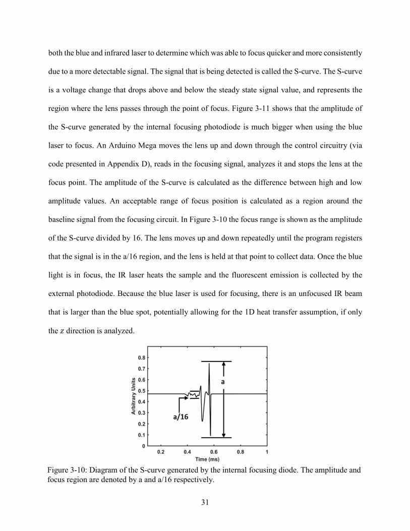
A custom unit was designed to house the lasers, optics, and electronics in a convenient unit.
The part shown below in Figure 3-7 was designed to hold the heating laser in line with the PHR’s
built in optical entry point for the infrared laser. When lined up correctly, the IR laser was directed
into the side of the PHR, through though optics, and out the lens above the sample, coming out at
the same point as the blue laser.
Figure 3-8: Experimental set up. PHR assembly with the amplified photodiode suspended above it. The IR laser is angled onto the sample from the side, but in the final version is held in a custom assembly.
Photodiode
PHR
Laser
Aixiz IR Laser
Figure 3-7: Custom designed piece to hold PHR laser assembly and the IR laser in line with the optics
PHR
Laser

30
Focusing
To achieve a small fluorescent spot size within the heating region on a variety of surfaces
a consistent focusing system is necessary. Focusing the blue laser also maximizes the power
absorbed by the fluorescent dye and increases its emission. A circuit developed by Diyouware [36]
controls the three laser diodes, moves the lens up and down, and outputs the photodiode signal
necessary for focusing. The movement of the lens is actuated by a voice coil actuator, where
motion is driven by a magnetic field and wound coil that produces a force when current runs
through it. This type of actuator allows for a very compact motion system with fine vertical
resolution for focusing the lasers. To focus the laser, we needed to develop a focusing code that
followed the algorithm Diyouware generated in their program. Diyouware developed a graphical
interface and program that could run focusing code, but for this project the Arduino code also
needed to control the motors. The first step in the focusing process is slowly moving the PHR lens
up and down, while recording the highest and lowest readings from the internal focusing
photodiode. The position of the lens is controlled by changing the pre-scaler on certain PWM
capable pins identified through the Arduino Mega datasheet. The duty cycle of the PWM signal is
sent through a MOSFET driver to a voice coil motor. The photodiode built into the PHR laser
assembly has four quadrants, shown in Figure 3-9, that collect reflected light; A, B, C, and D.
When (A+C) – (B+D) equals zero the laser is focused. As the lens moves up and down, a
voltage spike, called and S-curve, is generated by the photodiode. The PHR was focused using
Figure 3-9: Focusing states bases on the light reflected back onto the focusing diode. The left and right images result when the lens is too close or too far. The center is when the laser is in focus.
31
both the blue and infrared laser to determine which was able to focus quicker and more consistently
due to a more detectable signal. The signal that is being detected is called the S-curve. The S-curve
is a voltage change that drops above and below the steady state signal value, and represents the
region where the lens passes through the point of focus. Figure 3-11 shows that the amplitude of
the S-curve generated by the internal focusing photodiode is much bigger when using the blue
laser to focus. An Arduino Mega moves the lens up and down through the control circuitry (via
code presented in Appendix D), reads in the focusing signal, analyzes it and stops the lens at the
focus point. The amplitude of the S-curve is calculated as the difference between high and low
amplitude values. An acceptable range of focus position is calculated as a region around the
baseline signal from the focusing circuit. In Figure 3-10 the focus range is shown as the amplitude
of the S-curve divided by 16. The lens moves up and down repeatedly until the program registers
that the signal is in the a/16 region, and the lens is held at that point to collect data. Once the blue
light is in focus, the IR laser heats the sample and the fluorescent emission is collected by the
external photodiode. Because the blue laser is used for focusing, there is an unfocused IR beam
that is larger than the blue spot, potentially allowing for the 1D heat transfer assumption, if only
the 𝑧𝑧 direction is analyzed.
Figure 3-10: Diagram of the S-curve generated by the internal focusing diode. The amplitude and focus region are denoted by a and a/16 respectively.

32
Fluorescent Detection
With the lasers functioning and focused, it is then necessary to capture the emitted
fluorescence for analysis. To verify the emission wavelength and intensity, the emission from euro
the coin shown in Figure 3-12. The absolute intensity varies at each location due to varying
concentration of the dye across the sample. The first set up for collecting the emission was a fiber
optic cable positioned above a hole in the metal cover at the top of the laser assembly. Using a
spectrometer, the fiber was incrementally moved above the opening to locate the position of
highest transmitted fluorescent emission. Eventually, the fluorescent light emitted from the sample
was collected by removing the metal cover from the top of the PHR-803t to increase the amount
of fluorescence received by the photodetector and mounting an amplified Si photodiode (Thorlabs
PDA36A) directly above the laser assembly to collect as much light as possible. The photodiode
was used instead of the spectrometer to collect data because it is easier to collect pass the
photodiode output into the lock-in amplifier for comparison. With the spectrometer it would be
very difficult if not impossible to output a signal readable by the lock-in. The unfiltered light
entering the photodiode detector contains ambient light, 785nm IR light from the heating laser,
405 nm blue light from the probe laser, and fluorescent light.
Figure 3-11: Amplitude of the S-curve when focusing with the PHR's blue vs. focusing with the PHR's infrared laser

33
Approximately 0.6mL of a 1.075g/mL of the fluorescent Rhodamine B (RhB) dye was
deposited via dropper onto the Nordic Gold (89 Cu-5 Al-1 Sn) euro coin sample, left to dry, and
excited by the probe laser to induce fluorescent emission. The upper right area of the coin has a
different color due to a higher concentration of dye, with a dark ring around the area formed when
the drops of dye dried as seen in Figure 3-12. The fluorescence from the coin was analyzed by a
StellarNet Green-Wave spectrometer and shown in Figure 3-13 at four locations on the sample
Figure 3-13 shows the unfiltered light counts at the excitation and emission wavelengths when the
RhB was excited by the 405 nm laser, with the RhB’s peak emission near 610 nm when the. To
isolate the temperature dependent fluorescent emission, multiple optical filters were placed over
the photodiode. A 550nm longpass filter removed the blue light, and a 750nm shortpass filter
removed the IR laser emission. The adjustable gain photodiode (70dB, Thorlabs model mentioned
previously) amplified the light signal and output a time varying voltage signal proportional to the
fluorescence to be compared to the reference signal by the lock-in amplifier.
Figure 3-12: Image of coin with RhB deposited on surface. The color is different in certain areas due to the concentration of the dye regions. A and B show magnified images of the samples surface and how the distribution is uneven even at the mm scale, as well as the non-mirror like surface.

34
Fluorescent thermometry was chosen as the method of temperature sensing for multiple
reasons. Because the PHR laser assembly already contains a 405nm blue laser, it works well for
fluorescent methods. Because the blue laser can be used to induce fluorescence, it will work for
this method where the sensor does not need to touch the sample’s surface. Other methods for
measuring temperature would include analyzing the other side of the sample for a temperature
increase, thermocouple pads, or reflectance methods. These are more complicated to set up and
require a more complicated preparation process.
Lock-in Detection
The SR830 lock-in amplifier received the noisy signal from the amplified photodiode and
isolated the component at a frequency selected by the reference wave from the waveform generator.
The signal was sent by BNC to both the laser driver for modulating the IR laser, and to the lock-
in amplifier as the reference signal. The lock-in amplifier collected the fluorescent signal from the
photodiode, compared it to the reference signal from the waveform generator, then output the phase
delay between the two signals. The phase delay data (ϕtotal) was collected with MATLAB from
Figure 3-13: Graph of light intensity captured by a StellarNet Green-Wave spectrometer that measures between 350nm-1150nm. The peak at 405nm is the blue pump laser light, and the smaller peaks at 610nm are the fluorescent emission taken at four different locations on a sample.

35
the lock-in amplifier connected to the computer via a GPIB-USB connector. To determine the
phase delay (ϕinst) inherent to the electronics, the phase delay of the amplified photodiode
illuminated solely by modulated IR light was also measured over the frequency range. This
instrumentation phase delay was subtracted from the measured phase from the photodiode during
the fluorescent measurements, and the resulting phase delay (ϕthermal) of the temperature dependent
fluorescent signal was fit to a frequency domain model of the heat diffusion equation to determine
the thermal diffusivity.
Motors and Sample Movement
To move the sample beneath the PHR, while the PHR is held fixed, it is necessary to control
motors with a repeatable movement distance for each step. The Xbox disc player assembly
contains a motor to move the PHR laser assembly along the radius of the disc. This was that first
motor we attempted to use to move the samples. This motor is shown below in Figure 3-14, and
the data sheet is included in Appendix A. The motor was controlled via serial interface through an
Arduino program. The goal of controlling the motors was to input a desired direction and have the
motor move to that point. The program was set up to accept an input value of micrometers, then
the motor was stepped the according number of rotations that theoretically resulted in a
displacement of the entered distance. Via microscope and calibration slide, shown below in Figure
3-15, the distance of movement distance was verified and compared to the value that had been
entered into the Arduino control program. This was done in Matlab by measuring the pixel distance
moved and converting to micrometers based on the calibration ruler. The resulting distance
verification showed that the motor was not consistent in its movement. This is shown below in
Figure 3-16, where the actual location is shown to oscillate around the ideal value based on the

36
program input. Because of the imprecise control. A different motor was chosen to place in the
overall product assembly and move the sample.
Figure 3-14: Motor included in the Xbox assembly for moving the PHR laser assembly over a disc
Figure 3-15: Microscope images of calibration slide attached to motor to verify movement distance
Figure 3-16: Actual vs. Ideal motor location based on program input and measured location

37
4 RESULTS AND DISCUSSION
This chapter presents the thermal property results gathered on two different samples using
the FSTM and a heat transfer model from the literature. These samples include a 10 cent euro coin
and a thin film of uranium dioxide deposited on silicon. These samples were chosen because of
their rough surface for testing the capability of measuring minimally prepared samples, because of
their homogeneous structure, and to determine if the FSTM could be used on nuclear materials.
Each sample was analyzed to determine the thermal diffusivity and the methods unique to each
sample are discussed in the following sections. The collected data sometimes predicted values that
were outside of a physically possible range, or orders of magnitude off from the thermal diffusivity
values for a metallic material. These criteria were used as judgement to determine whether the data
would be used or not. The instrument phase delay was also affected by how the lasers were set up,
meaning it needed to be measured before each test to produce the most consistent data. If not done
correctly, the phase delay increased with frequency and the data needed to be retaken.
A heat transfer model from [39] was used to analyze the data. The model is a 3D Cartesian
representation of the frequency domain temperature variations on the surface of an 𝑛𝑛-layered
sample. The chosen model assumed no heat loss from the sample’s surface, because the analysis
in [39] found the effects of radiation and convection to be minimal in the frequency range of data
collection. It also assumes that the substrate is semi-infinite as long as the laser heating spot is 10
times larger than the thermal diffusion length. With the collected phase delay data, a property for

38
the sample was guessed, and an optimization routine varied the thermal diffusivity until the error
between the model and data points was minimized, with the output being the thermal diffusivity
that generated the curve with the least error. Thermal waves and the model are discussed in detail
in Appendix B.
The euro coin had experimental data collected by associates at Idaho National Labs or Utah
State University to provide a comparison with properties measured by the FSTM. A theoretical
models was also examined to calculate the effective thermal diffusivity of the euro based on
material properties and the definition of thermal diffusivity (𝛼𝛼 = 𝑘𝑘/𝜌𝜌𝑐𝑐𝑝𝑝 ), for comparison to
experimentally determined values. The method for collecting data on the FSTM and analyzing it
in MATLAB is discussed in Appendix E. The curve fitting process is discussed and the values &
methods of determining thermal diffusivity are presented in a tabular format. The results show that
the thermal diffusivity measurements were highly uncertain and require more in modeling and
instrumentation work to improve on them.
Euro Coin Data Collection
The first test sample for the FSTM was a 10 cent euro coin. Data was collected using the
external 90mW 780nm laser modulated between 80 Hz and 1 kHz, while the optical head’s blue
laser was used to induce fluorescence, and the optical head’s built in photodiode was used to focus
the blue laser on the sample. Above 1kHz, the data that was collected became too noisy and
inconsistent to calculate reasonable properties. On metallic samples, the thermal diffusivity is
relatively high and the phase delay will decrease slowly as frequency increases, as seen by the low
magnitude of the highest frequency phase delay (roughly -3º) shown in Figure 4-1. While the
decreasing trends in the total phase delay is apparent on the three samples, the trend in the net
phase delay (𝜙𝜙𝑡𝑡ℎ𝑒𝑒𝑒𝑒𝑒𝑒𝑒𝑒𝑒𝑒 = 𝜙𝜙𝑡𝑡𝑡𝑡𝑡𝑡𝑒𝑒𝑒𝑒 − 𝜙𝜙𝑖𝑖𝑖𝑖𝑖𝑖𝑡𝑡 ) is less consistent. The fluorescent component of the

39
phase delay makes up a small part of the overall signal, so when subtracting them, uncertainty is
larger relative to the net delay. At each location on the coin, and for each frequency, five seconds
of data was collected five times. The five points at each frequency were analyzed to find the mean
and standard deviation. Figure 4-2 presents thermal diffusivity measurements at these five spatially
distributed data points on the euro coin. Each location in Figure 4-2 has a frequency vs. phase
profile like that shown in Figure 4-1, which shows the different measured phases and best fit line
to equation 12. The fitting algorithm was a Levenberg Marquardt non-linear fitting process that
started with a preliminary thermal diffusivity input by the user. The starting value is used to
generate a plot of phase delay vs. frequency using the model detailed in the previous chapter. The
thermal diffusivity value is then varied until the error between the modeled curve and data points
is minimized.
The average measured value of the euro coin by FSTM was 𝛼𝛼=21±5 mm2/s, based on
measurements at multiple locations and the standard deviation of the five data points shown in
Figure 4-2. The goodness of fit was checked by calculating the square root of the sum of the
residuals squared for a property fit 10% above and below the value found by the Levenberg
Figure 4-1: Curve fit results for euro coin

40
Marquardt process (i.e. 19 and 23 mm2/s). The best fit line had a residual value of 3.61°, while the
higher and lower properties resulted in 3.62° and 3.62° respectively, verifying the goodness of the
initial fit. Thus, the fitting error was less significant than the standard deviation of multiple
measurements and will be ignored in the uncertainty analysis.
The thermal diffusivity of the coin was then compared to other established methods,
namely a thermal conductivity microscope (TCM, [24]) and laser flash. The TCM took several
spatial scans at 1, 2, 5, and 10 kHz on a third euro sample that was highly polished and coated with
approximately 35 nm of gold. The spatial scans involved in the TCM method involve a stationary
pump laser that heats the sample and a probe laser that scans away from the heating spot as the
phase delay between the input heating and temperature response is collected. This is shown in
Figure 1-6, and the results of the fitting based on models in [24] are shown in Figure 4-3. In Figure
4-3 the spatial scans at different frequencies are shown with the collected data shown as points and
the best fit results as a solid line. The resulting property was 19±3 mm2/s, where the uncertainty
represents the standard deviation of 15 measurements taken at different locations on the coin. Laser
flash was performed on a separate euro coin sample after both faces were polished and coated with
a thin layer of graphite. A Netzsch LFA 427 was used, resulting in 𝛼𝛼=30.4±0.1 mm2/s. On an
inhomogeneous sample, the comparison to LFA results would be irrelevant, since the FSTM
measures spatially varying properties and the LFA measures bulk. However, since the euro is
Figure 4-2: Image of sample with location of data points and resulting values overlaid.

41
homogeneous the thermal diffusivity results should be similar and are worth comparing. Finally
the Wiedemann-Franz law (𝑘𝑘 = 𝐿𝐿𝑑𝑑𝜎𝜎𝑒𝑒𝑒𝑒𝑒𝑒𝑒𝑒) [40] was used to approximate the electronic contribution
to the thermal conductivity, which is expected to dominate in a metal. Using a constant 𝜎𝜎𝑒𝑒𝑒𝑒𝑒𝑒𝑒𝑒 from
[41] and the Lorenz number (𝐿𝐿) of 2.44 ∗ 10−8 𝑊𝑊Ω𝐾𝐾−2, thermal conductivity over a range of
temperatures was determined. To compare the thermal diffusivity by FSTM, and TCM, to the
Wiedemann-Franz model, the definition of thermal diffusivity (𝛼𝛼 = 𝑘𝑘/𝜌𝜌𝑐𝑐𝑝𝑝 ) was used, where
density (𝜌𝜌) and specific heat (𝑐𝑐𝑝𝑝) were predicted from the alloy composition of Nordic Gold, which
is the name for the alloy used in euro coins. The results for the euro coin in Table 4-1 show that
the FSTM method found properties in the range of the other well-established methods, but with
higher uncertainty.
UO2 Data Collection
The second sample was a piece of silicon with a thin film of UO2 deposited on the top
surface. The sample is shown below in Figure 4-4. The RhB was deposited onto the surface in
successive drops, letting the toluene dissolving agent evaporate between applications.
Figure 4-3: Curve fit on data collected with TCM on euro coin

42
The data collected on the 500 nm UO2 film sample by the FSTM resulted in an effective
thermal diffusivity of the film/substrate of 𝛼𝛼𝑒𝑒𝑒𝑒𝑒𝑒=13mm2/s. Other measurements by the TCM on a
UO2 sample from the same wafer calculated the thermal diffusivity as 74.4 mm2/s. One key
difficulty with these measurements was the unknown thermal properties of the silicon substrate,
and because the film was so thin and the substrate so conductive, slight changes in substrate
properties had massive effects on the fitted value for the thermal diffusivity. This is a common
issue with inverse problems, as they are ill-posed. Additionally, the signal to noise ratio of the film
was lower than what was seen with the euro coin.
All the thermal conductivity values collected from each method on each sample are
presented in Table 4-1.
Table 4-1: Comparison of values calculated with various methods, all in units of mm2/s.
FSTM LFA TCM THEORETICAL
EURO 21±5 30.4±0.1 19±3 26
UO2 131 - 74.42 - 1 film/substrate values 2 film value based on k = 60 W/m-K for the Si substrate measured at INL
Figure 4-4: UO2 sample with RhB deposited on the surface
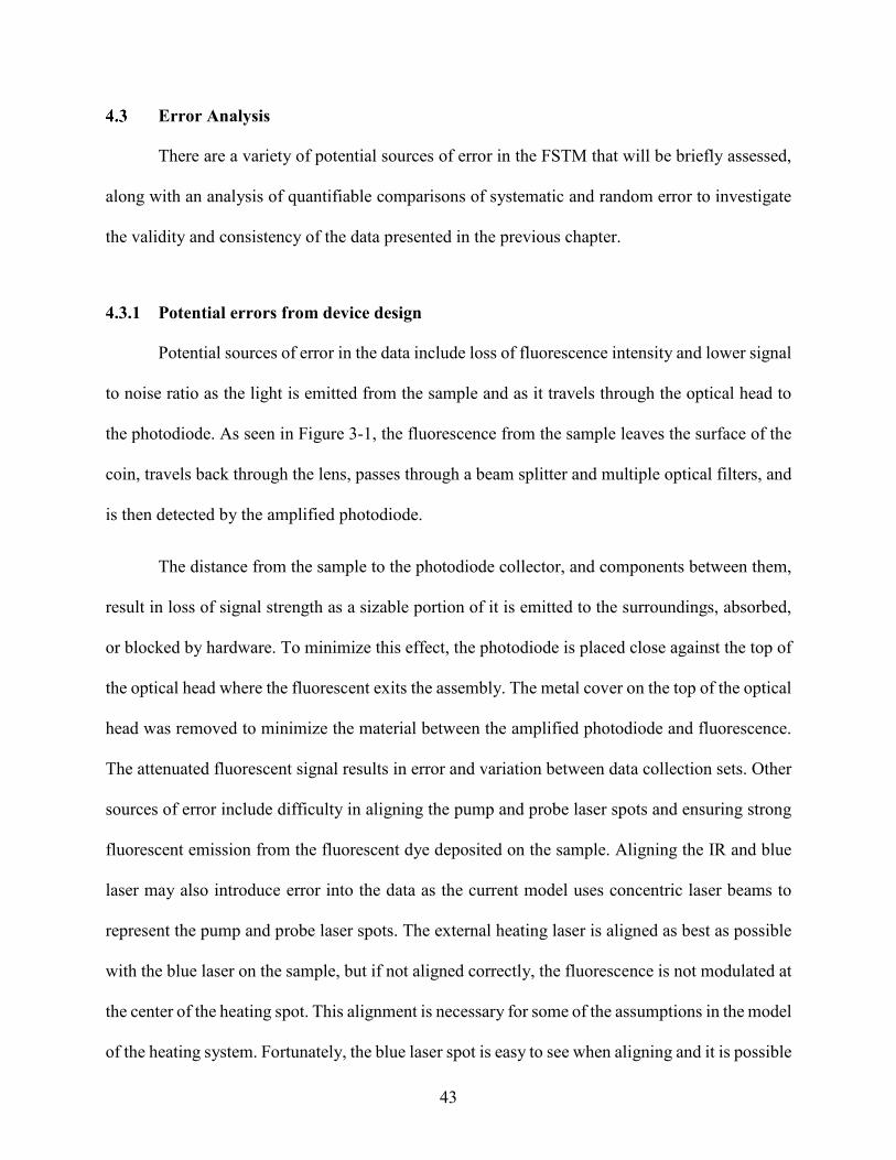
43
Error Analysis
There are a variety of potential sources of error in the FSTM that will be briefly assessed,
along with an analysis of quantifiable comparisons of systematic and random error to investigate
the validity and consistency of the data presented in the previous chapter.
4.3.1 Potential errors from device design
Potential sources of error in the data include loss of fluorescence intensity and lower signal
to noise ratio as the light is emitted from the sample and as it travels through the optical head to
the photodiode. As seen in Figure 3-1, the fluorescence from the sample leaves the surface of the
coin, travels back through the lens, passes through a beam splitter and multiple optical filters, and
is then detected by the amplified photodiode.
The distance from the sample to the photodiode collector, and components between them,
result in loss of signal strength as a sizable portion of it is emitted to the surroundings, absorbed,
or blocked by hardware. To minimize this effect, the photodiode is placed close against the top of
the optical head where the fluorescent exits the assembly. The metal cover on the top of the optical
head was removed to minimize the material between the amplified photodiode and fluorescence.
The attenuated fluorescent signal results in error and variation between data collection sets. Other
sources of error include difficulty in aligning the pump and probe laser spots and ensuring strong
fluorescent emission from the fluorescent dye deposited on the sample. Aligning the IR and blue
laser may also introduce error into the data as the current model uses concentric laser beams to
represent the pump and probe laser spots. The external heating laser is aligned as best as possible
with the blue laser on the sample, but if not aligned correctly, the fluorescence is not modulated at
the center of the heating spot. This alignment is necessary for some of the assumptions in the model
of the heating system. Fortunately, the blue laser spot is easy to see when aligning and it is possible

44
to place the blue laser in the center of the IR heating spot via visual inspection of a faint red dot
emitted from the 780nm diode in addition to the invisible IR light. The red light was a higher
wavelength than the fluorescence and was filtered out before reaching the photodiode.
4.3.2 Statistical error analysis
To assess the results and determine the validity of the FSTM’s thermal diffusivity values,
a t-test at the 5% confidence interval was done on the sets of data from the FSTM, LFA, and TCM
for the euro. Even though the FSTM and LFA measure different property scales, the results worth
comparing for the euro because it is homogeneous and should result in similar results. A t-test
measures two sets of data to evaluate the null hypothesis that the difference in the means is zero.
If the null hypothesis is not rejected, then the differences in the mean thermal diffusivity values
can be attributed to randomness and not to systematic (or instrument related) errors. To compute
the t value in a two sample t-test, the equation 15 is used to compare the difference in the mean to
the difference in the magnitude of the normalized variance in each data set.
𝑡𝑡 =𝛼𝛼1��� − 𝛼𝛼2���
�𝑠𝑠𝛼𝛼12
𝑛𝑛 +𝑠𝑠𝛼𝛼22𝑚𝑚
(2)
The resulting t-values are compared to a t distribution value based on the percent
probability that the null hypotheses can be rejected. If the calculated 𝑡𝑡 value is less than the t
distribution in Table 4.4 of [43], then the null hypotheses may not be rejected and the differences
in the measurements from different devices can be attributed to randomness. Table 4-2 presents
the t-test results for the euro coin between each of the three methods used to measure the thermal
diffusivity. As seen in the t-test results, the measurements from the FSTM and the TCM are close
enough in the mean thermal diffusivity that the difference can be attributed to random error. But

45
when comparing the FSTM to the LFA the error is more significant than randomness. However,
the similarities in the FSTM and TCM measurements bodes well, as they are both microscopic
measurements of 𝛼𝛼.
Table 4-2: T-test results for the euro. If the null hypothesis is not rejected, the results are close enough between the systems that the difference can be attributed to random error.
EURO t Null Hypothesis Result
FSTM-LFA 3.9 Reject Difference due to system error
FSTM-TCM 0.7 Not rejected Difference within random error
LFA-TCM 11.3 Reject Difference due to system error
Based on this statistical analysis, we can conclude that the measurements of the FSTM are
statically comparable to those by TCM when using the same heat transfer model. However, there
is a significant amount of uncertainty on the FSTM measurements (~25% from the standard
deviation of measured values, with uncertainty to increase when considering modeling effects).
Cost Assessment
Because the development of the FSTM was partially focused on providing a cheap device,
the cost of the different components must be considered and is presented in Appendix C. The vast
majority of the cost is comprised of the lock-in amplifier. With the future development of a cheap,
specialized lock-in, the goal of a more cost-effective thermal characterization microscope can more
fully be realized. Among other methods researched, this FSTM method is least expensive.
Difficulties with the PHR-803t include a weak infrared laser and the limit of only turning one laser
on at a time with the built-in control circuitry. To overcome, this an aftermarket IR laser was

46
incorporated into the set up and the blue laser is controlled through the built-in circuitry. The
optical head’s infrared laser will then be replaced with a more powerful laser diode. The resulting
total cost is shown in the Bill of Materials in the Appendix C.

47
5 CONCLUSION
The thermal diffusivity value found by the FSTM microscope fall between the measured
values from the other experimental data (LFA, TCM) but are statistically uncertain, with only one
result falling within random error instead of systematic or modeling error. These measurements
were based on statistical t-tests. When compared to the LFA the difference is statistically outside
random variation and indicates error within the FSTM system, even though it is a homogeneous
sample with consistent properties throughout. But interestingly in the t-test comparison between
the LFA and TCM (both well-established methods), the results were outside the range of random
error as well, even though they were both measuring a homogeneous sample. Overall, the property
measurements are highly uncertain and the device and indicate that the heat transfer model likely
doesn’t work and needs further refinement.
Comparing the physical functioning of the different methods, TCM requires polishing the
sample down and coating it in a reflective metal. These requirements are not always feasible,
because it is possible that the surface to study is rough and polishing may remove the structures of
interest. For the method demonstrated in this thesis, surface preparation was limited to preparing
the fluorescent dye solution, depositing an adequate amount onto the sample, and letting it
evaporate. The FSTM method does not require access to both sides of the sample, as both lasers
and detecting instrumentation are suspended above one side of it. The sample used to collect data
was not polished, but the modeling may need further investigation to work with rough sample
48
surfaces. There is a need for refinement to achieve more certain results, especially in preparation
for nuclear fuel analysis.
The objectives of the project included heating, scanning, collecting data, using the
appropriate model for the system, and calculating properties on a known and unknown material
sample. The device hardware and instrumentation performs as expected, but the accuracy of
thermal measurements is not yet confirmed. The device was verified to heat samples adequately
using an inexpensive infrared laser by shining it on a thermocouple for measuring a temperature
change. The motor scanning is on the desired length scale, but the step size is not as repeatable as
hoped. The device was also able to collect the necessary fluorescent data via photodiode after
experimenting with the best way to capture as much fluorescence as possible with the PHR, which
ended up being an open PHR assembly with the amplified photodiode suspended above it, placed
against the optical filters. The heat transfer in the sample was modeled based on the work in the
literature that represented a sample with a thin layer on it that absorbs modulated heating from a
laser. The model parameters that represented the density and specific heat of the material were
adjusted to match the samples analyzed in this project. The FSTM was used to collect data and
calculate the properties of a known material (the euro), and a material of unknown properties,
related to nuclear fuels (UO2). The results for the euro was closer to other methods, but highly
uncertain, and the UO2 piece was much higher than the data collected by TCM. While some results
were in between or near those from the other methods, the variation in most of them indicated
necessary systematic changes to increase the consistency of the results.
Limitations and Future Work
The results largely indicate substantial error in the system and/or model. The results
presented in the previous chapter were achieved after many attempts at collecting data that related

49
to properties on the right order of magnitude. It is not yet consistent enough for commercial use.
Sometimes the changes between tests that resulted in unreasonable and reasonable results were
unnoticeable, and it is difficult to articulate or quantify why some tests came out well and some
did not. The phase delay data for the euro coin lined up well with the best fit curve from the model
and the predicted curve was within the uncertainty of the data points.
The heat transfer model needs to be examined in depth to investigate the following:
• Incorporating surface roughness effects into the model, as measuring rough surfaces is an
advantage of the FSTM.
• Finding properties of RhB and incorporating thin RhB layer into the model.
• Modeling contact resistance, like the interface between the RhB and the substrate.
• Additional investigation of no heat loss assumption
• Role of surface roughness on applicability of existing heat transfer models.
The following lists future work to refine the instrumentation:
• Examining alternates to the PHR-803t to see if there is a better way to capture fluorescent
data. One option for this is using just an Aixiz 405nm blue laser instead of the PHR-803t
and putting the photodiode closer to the sample surface so that the fluorescence is not
blocked by hardware.
• Future work also includes refining the assembly that houses all the electronics and
components together.
• Developing circuitry and integration of a cheaper lock-in amplifier and waveform
generator.
• Testing the FSTM on more materials to refine the range of materials that will work well
with modulated fluorescent methods.

50
• Investigating movement of the PHR-803t lens in other axes to potentially offset the laser
spot for spatially offset measurements, Diyouware [36] mentions the lens pins can be used
to do so.
• Designing and testing a Nema 17 powered lead screw motion system.
• Taking measurements with the TCM may also be performed for comparison with the
results collected on a standard reference material.
• Finally, because of the variation between the various measurement methods, the systematic
error of the FSTM needs to be determined based on round robin measurements of standard
reference samples.

51
REFERENCES
[1] Lakowicz, J.R., Principles of Fluorescence Spectroscopy. 2006: Springer US.
[2] Banerjee, S. and T.R.G. Kutty, Challenges in Nuclear Materials. Science and Culture, 2013. 79.
[3] Nakamura, J., et al., Thermal Conductivity Change in High Burnup MOX Fuel Pellet. Journal of Nuclear Science and Technology, 2009. 46(9): p. 944-952.
[4] Zinkle, S.J., et al., Accident Tolerant Fuels for LWRs: A Perspective. Journal of Nuclear Materials, 2014. 448(1-3).
[5] Tonks, M.R., et al., Mechanistic materials modeling for nuclear fuel performance. Annals of Nuclear Energy, 2017. 105(Supplement C): p. 11-24.
[6] Cahill, D.G., Thermal conductivity measurement from 30 to 750 K: the 3ω method. Review of Scientific Instruments, 1990. 61(2): p. 802-808.
[7] Parker, W.J., et al., Flash Method of Determining Thermal Diffusivity, Heat Capacity, and Thermal Conductivity. Journal of Applied Physics, 1961. 32(9): p. 1679-1684.
[8] Cahill, D.G., Analysis of heat flow in layered structures for time-domain thermoreflectance. Review of Scientific Instruments, 2004. 75(12): p. 5119-5122.
[9] White, J.T., et al., Thermophysical properties of U3Si2 to 1773K. Journal of Nuclear Materials, 2015. 464: p. 275-280.
[10] Whittle, K., Nuclear fuel, part 2: operational effects, in Nuclear Materials Science. 2016, IOP Publishing. p. 4-1-4-18.
[11] Abad, B., D.A. Borca-Tasciuc, and M.S. Martin-Gonzalez, Non-contact methods for thermal properties measurement. Renewable and Sustainable Energy Reviews, 2017. 76: p. 1348-1370.
[12] Jo, S., et al., Development of an online nuclear materials thermo-physical property database (THERPRO). Journal of the Korean Physical Society, 2011. 59(23): p. 1107-1110.

52
[13] Zhang, Y., et al., A noncontact thermal microprobe for local thermal conductivity measurement. Review of Scientific Instruments, 2011. 82(2): p. 024902.
[14] Zhang, Y., et al., A microprobe technique for simultaneously measuring thermal conductivity and Seebeck coefficient of thin films. Applied Physics Letters, 2010. 96(6): p. 062107.
[15] Chirtoc, M., et al., 1ω, 2ω, 3ω Scanning Thermal Microscopy (SThM) and combinations with thermographic, radiometric, pyroelectric and thermoelastic techniques; Principles and applications. Advanced Techniques and Applications on Scanning Probe Microscopy, 2008: p. 197-247.
[16] Takahashi, Y. and M. Murabayashi, Measurement of Thermal Properties of Nuclear Materials by Laser Flash Method. Journal of Nuclear Science and Technology, 1975. 12(3): p. 133-144.
[17] Rosencwaig, A., et al., Detection of thermal waves through optical reflectance. Applied Physics Letters, 1985. 46(11): p. 1013-1015.
[18] Cahill, D. and R. Pohl, Thermal Conductivity of Amorphous Solids above the Plateau. Physical review. B, Condensed matter, 1987. 35(8): p. 4067-4073.
[19] Shrestha, K. and K. Gofryk, Thermal conductivity of actinide materials measured using the 3 ω method. APS March Meeting, 2017.
[20] Malen, J.A., et al., Optical Measurement of Thermal Conductivity Using Fiber Aligned Frequency Domain Thermoreflectance. Journal of Heat Transfer, 2011. 133(8): p. 081601-081601-7.
[21] Schmidt, A.J., R. Cheaito, and M. Chiesa, A frequency-domain thermoreflectance method for the characterization of thermal properties. Review of Scientific Instruments, 2009. 80(9): p. 094901.
[22] Hua, Z., et al., Spatially localized measurement of thermal conductivity using a hybrid photothermal technique. Journal of Applied Physics, 2012. 111(10): p. 103505.
[23] Labratories, I.N., Laboratory Directed Research and Development 2017 Annual Summary Report. 2017.
[24] Hurley, D.H., et al., Local measurement of thermal conductivity and diffusivity. Review of Scientific Instruments, 2015. 86(12).
[25] Dilhaire, S., et al., Heterodyne picosecond thermoreflectance applied to nanoscale thermal metrology. Journal of Applied Physics, 2011. 110(11): p. 114314.
[26] Liu, X.F., et al., Thermal conductivity measurement of individual CdS nanowires using microphotoluminescence spectroscopy. Journal of Applied Physics, 2010. 108(5): p. 054310.

53
[27] Munro, T., et al., Thermophysical properties of thin fibers via photothermal quantum dot fluorescence spectral shape-based thermometry. International Journal of Heat and Mass Transfer, 2017. 112: p. 1090-1097.
[28] Kasha, M., Characterization of electronic transitions in complex molecules. Discussions of the Faraday Society, 1950. 9(0): p. 14-19.
[29] Reshma, V.G. and P.V. Mohanan, Quantum dots: Applications and safety consequences. Journal of Luminescence, 2018. 205.
[30] Resch-Genger, U., et al., Quantum dots versus organic dyes as fluorescent labels. Nat Meth, 2008. 5(9): p. 763-775.
[31] Munro, T., et al., CdSe/ZnS quantum dot fluorescence spectra shape-based thermometry via neural network reconstruction. Journal of Applied Physics, 2016. 119(21): p. 214903.
[32] Glawdel, T., et al., Photobleaching absorbed Rhodamine B to improve temperature measurements in PDMS microchannels. Lab on a Chip, 2009. 9(1): p. 171-174.
[33] Maruyama, H., R. Kariya, and F. Arai, Evaluation of thermal conductivity of single carbon nanotubes in air and liquid using a fluorescence temperature sensor. Applied Physics Letters, 2013. 103(16): p. 161905.
[34] Moeken, H.H.P. and W.A.H. Van Neste, Absorptiometric determination of microgram amounts of uranium with Rhodamine B. Analytica Chimica Acta, 1967. 37: p. 480-483.
[35] Lietzke, A.F., Simplified Analysis of Nuclear Fuel Pin Swelling, in NASA-TN-D-5609. 1970, NASA: Cleveland, Ohio.
[36] Victor. Diyouware TwinTeeth: The PCB mini-factory. 2013 [cited 2017; Available from: http://www.diyouware.com/.
[37] Walker, G.W., et al., Quantum-dot optical temperature probes. Applied Physics Letters, 2003. 83(17): p. 3555-3557.
[38] Liu, L., et al., Temperature-sensitive photoluminescent CdSe-ZnS polymer composite film for lock-in photothermal characterization. Journal of Applied Physics, 2016. 119(22): p. 224902.
[39] Hua, Z., Hybrid Photothermal Technique for Microscale Thermal Conductivity Measurement, in Mechanical and Aerospace Engineering. 2013, Utah State University.
[40] Kim, H.-S., et al., Characterization of Lorenz number with Seebeck coefficient measurement. APL Materials, 2015. 3(4): p. 041506.
[41] Kolyshkin, A., et al. Determination of electrical conductivity of metal plates using planar spiral coils. in Proceedings of the 13th WSEAS international conference on Systems. 2009.

54
[42] Cupronickel Properties. Available from: http://www.matweb.com/search/DataSheet.aspx?MatGUID=4fb6ab47b8784e868bc270d230da8109&ckck=1.
[43] Richard S. Figliola , D.E.B., Theory and Design for Mechanical Measurements. 2015.
[44] Almond, D.P. and P.M. Patel, Photothermal Sciences and Techniques. Physics and its Applications, ed. E.R. Dobbs and S.B. Palmer. Vol. 10. 1996: Chapman & Hall.
[45] Pilla, V., et al., Photothermal Spectroscopic Characterization in CdSe/ZnS and CdSe/CdS Quantum Dots: A Review and New Applications, in Quantum Dots: A Variety of New Applications, A. Al-Ahmadi, Editor. 2012.
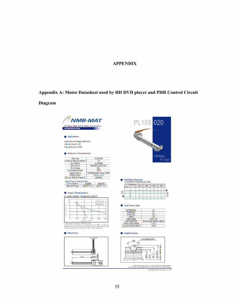
55
APPENDIX
Appendix A: Motor Datasheet used by HD DVD player and PHR Control Circuit
Diagram
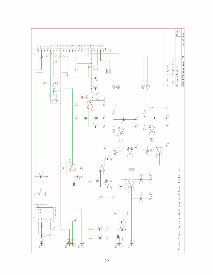
56

57
Appendix B: Modeling
This section describes some fundamentals of periodic heat transfer analysis and the model
that was used in the data analysis for this project. Periodic heating and mathematical analysis in
the frequency domain has been used in many property characterization techniques, like those
discussed in section 1.2.2, and simplifies the data collection involved. It is not necessary to
measure the absolute temperature value and its transient change, but only the variation from steady
state temperature. Therefore, the temperature of the sample or temperature fluorescence relation
does not need to be calibrated. The model discussed in this chapter discusses the heat transfer
analysis in the frequency domain for a laser heated sample in 3 dimensions and the capability of
including different material layers and thicknesses within the sample.
Introduction to Periodic Heat Absorption and Transfer
As an introduction to periodic heating analysis, often characterized as thermal waves, we
will first look at an isotropic homogeneous semi-infinite medium [44] that is periodically heated
by a modulated laser.
In a 1D model the laser is treated as a boundary condition with the representation of
𝜕𝜕2𝑑𝑑𝜕𝜕𝑥𝑥2
−1𝛼𝛼𝜕𝜕𝑑𝑑𝜕𝜕𝑡𝑡
= 0 (1)
−𝑘𝑘𝜕𝜕𝑑𝑑𝜕𝜕𝑥𝑥
|𝑥𝑥=0 =𝑄𝑄𝑡𝑡2
[1 + cos(𝜔𝜔𝑡𝑡)] (2𝑎𝑎)
𝜕𝜕𝑑𝑑𝜕𝜕𝑥𝑥
|𝑥𝑥→∞ = 0 (2𝑏𝑏)
𝑑𝑑(𝑥𝑥, 0) = 𝑑𝑑𝑖𝑖 (2𝑐𝑐)
with 𝑄𝑄𝑡𝑡/2 shown in equation 2a representing the laser power and DC offset when distributed to
the first term in brackets, and 𝜔𝜔 the frequency of modulation. The transient heat equation in one
direction will be used to solve for the temperature profile in this scenario. The boundary condition

58
will equate the conduction into the material to the periodic thermal energy from the laser at the
surface.
−𝑘𝑘𝜕𝜕𝑑𝑑𝜕𝜕𝑥𝑥
=𝑄𝑄𝑡𝑡2
[1 + cos(𝜔𝜔𝑡𝑡)] = Re �𝑄𝑄𝑡𝑡2
[1 + exp(𝑗𝑗𝜔𝜔𝑡𝑡)]� (3)
where 𝑘𝑘 represents the thermal conductivity of the material. The real part of the heating can be
broken down into steady and transient terms, 𝑄𝑄𝑜𝑜2
and 𝑄𝑄𝑜𝑜2
exp(𝑗𝑗𝜔𝜔𝑡𝑡) respectively, when 𝑄𝑄𝑜𝑜2
is
distributed through the expression. Only the transient part will be analyzed in the following
solution. To solve the transient 1-D heat equation we will assume the periodic component solution
is of this form:
𝑑𝑑(𝑥𝑥, 𝑡𝑡) = 𝑑𝑑𝑅𝑅 �𝑑𝑑�(𝑥𝑥)𝑅𝑅𝑥𝑥𝑒𝑒(𝜔𝜔𝑡𝑡)� (4)
The quasi-steady solution to equation 1 becomes
𝑑𝑑(𝑥𝑥) = 𝐴𝐴 exp(−𝜎𝜎𝑥𝑥) + 𝐵𝐵 exp(𝜎𝜎𝑥𝑥) (5)
𝜎𝜎 = (1 + 𝑗𝑗) �𝜔𝜔𝑤𝑤𝛼𝛼
�12 (6)
where 𝐴𝐴 and 𝐵𝐵 are arbitrary constants and 𝜎𝜎 is defined in equation 6. The sample in the case of
equation 2 is represented as a semi-infinite media. Assuming that 𝑑𝑑(𝑥𝑥) is finite as 𝑥𝑥 goes to
infinity, 𝐵𝐵 is zero. The boundary condition in equation 2a-c represents the heat from the laser being
equal to the conduction into the material at the surface and can be used to solve for the constant 𝐴𝐴
in equation 5. Solving the equation out it results in
𝑑𝑑(𝑥𝑥, 𝑡𝑡) =𝑄𝑄𝑡𝑡
2�𝜌𝜌𝑐𝑐𝑘𝑘𝜔𝜔exp �−
𝑥𝑥𝜇𝜇� exp �𝑗𝑗 �𝜔𝜔𝑡𝑡 −
𝑥𝑥𝜇𝜇−𝜋𝜋4�� (7)

59
𝜇𝜇 = �2𝛼𝛼𝜔𝜔
(8)
where 𝜌𝜌, 𝑐𝑐𝑝𝑝, and 𝑘𝑘 represent density, specific heat, and thermal conductivity of the material and 𝜇𝜇
is the thermal diffusion length of the periodic wave. The thermal diffusion length represents how
far into the material the temperature change penetrates, characterizes the thermal wave, and is a
function of the thermal diffusivity of the sample and frequency of the heating laser. This simple
model will not work to calculate the phase delay of thermal waves, because with our method of
temperature sensing, we can only measure the temperature at the surface of the material when 𝑥𝑥 =
0. In this is the case, the terms with 𝑥𝑥 disappear and the phase delay at the surface is a constant
𝜋𝜋/4. Additionally, this model does not work because of its 1D nature, the fact that it only accounts
for a single material layer, and that the spatial distribution of the laser beam is not considered. In
the experiments of the current work, the sample has a very thin layer of the fluorescent dye on the
surface. Other works indicate that the quantum dot particles do not contribute significantly to the
thermal diffusivity, and the RhB dye particles are assumed similar enough that it also applies [45].
Heat Diffusion Model
To relate the temperature dependent fluorescent intensity to the thermal diffusivity of the
sample, it is necessary to solve the inverse problem applied to the heat diffusion equation and
account for the heating depth in the sample and layered dye to find a property dependent phase
delay. In [22, 39], a 3D model is developed that uses a heat generation expression in the heat
diffusion equation to represent the absorption of the IR laser. This model was used for frequency
domain experiments and can analyze the data taken with the FSTM. The model was developed to
account for layered samples, and it can represent the fluorescent dye layered on the surface of the
sample or it can be considered as two layers with similar properties. The single layer form was

60
used in this experiment based on the assumption that all of the infrared heating passed through the
fluorescent layer and was absorbed by the sample. This was assumed because the Rhodamine was
deposited as a mixture with toluene and then the toluene evaporated off of the sample, leaving only
the small RhB particles. This model was developed in 3D to account for a spatial separation of the
pump and probe laser if necessary. This may be possible in future iterations of the device, where
the IR laser spot can be moved to produce a spatial offset between the laser spots. The governing
equation of the 3D model is as follows, and the physical representation of it is shown in Figure
A-1,
𝑘𝑘𝑒𝑒𝑖𝑖𝑓𝑓𝑑𝑑𝑒𝑒,𝑖𝑖𝑓𝑓 − 𝜌𝜌𝑒𝑒𝑐𝑐𝑒𝑒�̇�𝑑𝑒𝑒 = 𝑄𝑄𝑒𝑒 (9)
𝑘𝑘𝑖𝑖𝑖𝑖𝑓𝑓𝑑𝑑𝑖𝑖,𝑖𝑖𝑓𝑓 − 𝜌𝜌𝑖𝑖𝑐𝑐𝑖𝑖�̇�𝑑𝑖𝑖 = 𝑄𝑄𝑖𝑖 (10)
with the following terms for the Gaussian distributed heat sources,
𝑄𝑄𝑒𝑒 =𝑃𝑃𝛼𝛼𝑒𝑒�1 − 𝑑𝑑𝑒𝑒�
𝜋𝜋𝑎𝑎1𝑎𝑎2exp�−
𝑥𝑥12
𝑎𝑎12−𝑥𝑥22
𝑎𝑎22− 𝛼𝛼𝑒𝑒𝑥𝑥3� �
12
+14
(exp(𝑖𝑖𝜔𝜔𝑡𝑡) + exp(−𝑖𝑖𝜔𝜔𝑡𝑡))� (11)
where P is the power of the pump laser and 𝑎𝑎1 and 𝑎𝑎2 are the major and minor axes of the heating
laser spot, and R is the reflectivity on the surface of layers. The subscript 𝑓𝑓 represents the film,
and 𝑠𝑠 represents the substrate, with ℎ representing the film thickness. This model can also consider
anisotropic thermal conductivity, with the directions represented by subscripts 𝑖𝑖 and 𝑗𝑗, but was
considered isotropic for the Nordic Gold coin. The surface temperature of the sample is derived in
Fourier space as 𝑑𝑑𝑡𝑡� (𝜉𝜉1, 𝜉𝜉2) with 𝜉𝜉1 and 𝜉𝜉1 and 𝜉𝜉2 representing the integral variables. With the
necessary boundary conditions, the inverse Fourier transform is performed numerically on
equation 11.
𝑑𝑑𝑡𝑡 =1
2𝜋𝜋� 𝑑𝑑𝑡𝑡� (𝜉𝜉1, 𝜉𝜉2) exp[𝑖𝑖(𝜉𝜉1𝑥𝑥1 + 𝜉𝜉2𝑥𝑥2)]𝑑𝑑𝜉𝜉1 𝑑𝑑𝜉𝜉2
∞
−∞(12)

61
In transform space, the solution is
𝑑𝑑𝑒𝑒� = 𝐴𝐴 exp�−𝜂𝜂𝑒𝑒𝑥𝑥3� + 𝐵𝐵 exp�𝜂𝜂𝑒𝑒𝑥𝑥3� +𝐸𝐸 exp�−𝛼𝛼𝑒𝑒𝑥𝑥3� (13)
𝑑𝑑𝑖𝑖� = 𝐶𝐶 exp�−𝜂𝜂𝑖𝑖(𝑥𝑥3 − ℎ)� + 𝐷𝐷 exp�𝜂𝜂𝑖𝑖(𝑥𝑥3 − ℎ)�+𝐹𝐹 exp�−𝛼𝛼𝑖𝑖(𝑥𝑥3 − ℎ)� (14)
where coefficients 𝐴𝐴, 𝐵𝐵, 𝐶𝐶, 𝐷𝐷, and 𝐸𝐸 and the 𝜂𝜂 values are found with the mathematical methods
shown in Appendix B of [39]. The model produces a curve like that shown in Figure A-2, where
the properties of the euro coin were input as parameters and the film and substrate where assumed
to be one material.
Figure A-1: Set up of system to be analyzed. The heating first hits the top layer of RhB particles and is transmitted to the substrate. The model can account for two layers denoted by f for film and s for substrate
Figure A-2: Output of heat diffusion model using properties of Nordic gold, from 1 to 1000Hz

62
More detail is provided here on the model.
Governing equations:
𝑘𝑘𝑒𝑒𝑖𝑖𝑓𝑓𝑑𝑑𝑒𝑒,𝑖𝑖𝑓𝑓 − 𝜌𝜌𝑒𝑒𝑐𝑐𝑒𝑒�̇�𝑑𝑒𝑒 = 𝑄𝑄𝑒𝑒 (15)
𝑘𝑘𝑖𝑖𝑖𝑖𝑓𝑓𝑑𝑑𝑖𝑖,𝑖𝑖𝑓𝑓 − 𝜌𝜌𝑖𝑖𝑐𝑐𝑖𝑖�̇�𝑑𝑖𝑖 = 𝑄𝑄𝑖𝑖 (16)
Heat source terms:
𝑄𝑄𝑒𝑒 =𝑃𝑃𝛼𝛼𝑒𝑒�1 − 𝑑𝑑𝑒𝑒�
𝜋𝜋𝑎𝑎1𝑎𝑎2exp�−
𝑥𝑥12
𝑎𝑎12−𝑥𝑥22
𝑎𝑎22− 𝛼𝛼𝑒𝑒𝑥𝑥3� �
12
+14
(exp(𝑖𝑖𝜔𝜔𝑡𝑡) + exp(−𝑖𝑖𝜔𝜔𝑡𝑡))� (17)
𝑄𝑄𝑖𝑖 =𝑃𝑃𝛼𝛼𝑖𝑖�1 − 𝑑𝑑𝑒𝑒�(1 − 𝑑𝑑𝑖𝑖) exp�−𝛼𝛼𝑒𝑒𝑓𝑓ℎ�
𝜋𝜋𝑎𝑎1𝑎𝑎2exp�−
𝑥𝑥12
𝑎𝑎12−𝑥𝑥22
𝑎𝑎22− 𝛼𝛼𝑖𝑖(𝑥𝑥3 − ℎ)��
12
+14
(exp(𝑖𝑖𝜔𝜔𝑡𝑡) + exp(−𝑖𝑖𝜔𝜔𝑡𝑡))� (18)
Boundary conditions:
−𝑘𝑘𝑒𝑒3𝑖𝑖𝜕𝜕𝑑𝑑𝑒𝑒𝜕𝜕𝑧𝑧
|𝑧𝑧=0 = 0 (19)
𝑘𝑘𝑒𝑒3𝑖𝑖𝜕𝜕𝑑𝑑𝑒𝑒𝜕𝜕𝑧𝑧
|𝑧𝑧=ℎ = 𝑘𝑘𝑖𝑖3𝑖𝑖𝜕𝜕𝑑𝑑𝑖𝑖𝜕𝜕𝑧𝑧
|𝑧𝑧=ℎ (20)
−𝑑𝑑𝑡𝑡ℎ𝑘𝑘𝑖𝑖3𝑖𝑖𝜕𝜕𝑑𝑑𝑒𝑒𝜕𝜕𝑧𝑧
|𝑧𝑧=ℎ = 𝑑𝑑𝑒𝑒 − 𝑑𝑑𝑖𝑖 (21)
Normalization factors in 3 and 4 come from the following
�𝑄𝑄𝑒𝑒𝑑𝑑𝑑𝑑 = 𝑃𝑃�1 − 𝑑𝑑𝑒𝑒� (22)
�𝑄𝑄𝑖𝑖𝑑𝑑𝑑𝑑 = 𝑃𝑃�1 − 𝑑𝑑𝑒𝑒�(1 − 𝑑𝑑𝑖𝑖) exp�−𝛼𝛼𝑒𝑒ℎ� (23)
which implies
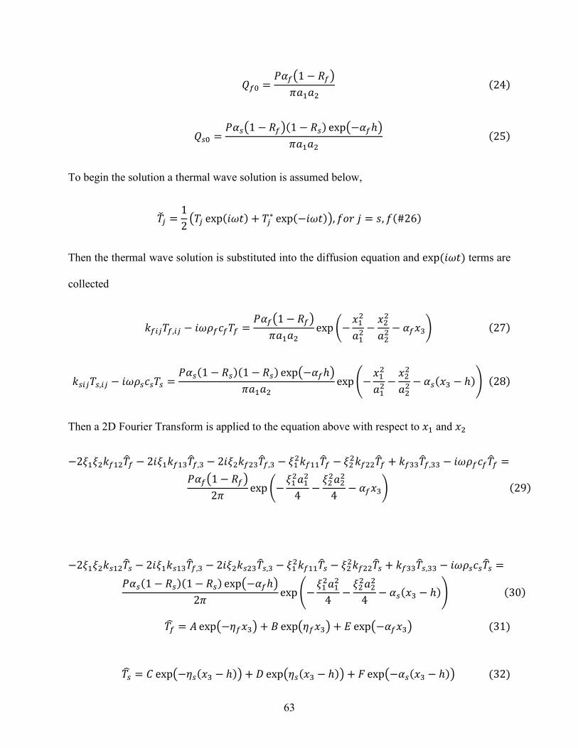
63
𝑄𝑄𝑒𝑒0 =𝑃𝑃𝛼𝛼𝑒𝑒�1 − 𝑑𝑑𝑒𝑒�
𝜋𝜋𝑎𝑎1𝑎𝑎2(24)
𝑄𝑄𝑖𝑖0 =𝑃𝑃𝛼𝛼𝑖𝑖�1 − 𝑑𝑑𝑒𝑒�(1 − 𝑑𝑑𝑖𝑖) exp�−𝛼𝛼𝑒𝑒ℎ�
𝜋𝜋𝑎𝑎1𝑎𝑎2(25)
To begin the solution a thermal wave solution is assumed below,
𝑑𝑑�𝑓𝑓 =12�𝑑𝑑𝑓𝑓 exp(𝑖𝑖𝜔𝜔𝑡𝑡) + 𝑑𝑑𝑓𝑓∗ exp(−𝑖𝑖𝜔𝜔𝑡𝑡)�,𝑓𝑓𝑓𝑓𝑓𝑓 𝑗𝑗 = 𝑠𝑠, 𝑓𝑓(#26)
Then the thermal wave solution is substituted into the diffusion equation and exp (𝑖𝑖𝜔𝜔𝑡𝑡) terms are
collected
𝑘𝑘𝑒𝑒𝑖𝑖𝑓𝑓𝑑𝑑𝑒𝑒,𝑖𝑖𝑓𝑓 − 𝑖𝑖𝜔𝜔𝜌𝜌𝑒𝑒𝑐𝑐𝑒𝑒𝑑𝑑𝑒𝑒 =𝑃𝑃𝛼𝛼𝑒𝑒�1 − 𝑑𝑑𝑒𝑒�
𝜋𝜋𝑎𝑎1𝑎𝑎2exp �−
𝑥𝑥12
𝑎𝑎12−𝑥𝑥22
𝑎𝑎22− 𝛼𝛼𝑒𝑒𝑥𝑥3� (27)
𝑘𝑘𝑖𝑖𝑖𝑖𝑓𝑓𝑑𝑑𝑖𝑖,𝑖𝑖𝑓𝑓 − 𝑖𝑖𝜔𝜔𝜌𝜌𝑖𝑖𝑐𝑐𝑖𝑖𝑑𝑑𝑖𝑖 =𝑃𝑃𝛼𝛼𝑖𝑖(1 − 𝑑𝑑𝑖𝑖)(1 − 𝑑𝑑𝑖𝑖) exp�−𝛼𝛼𝑒𝑒ℎ�
𝜋𝜋𝑎𝑎1𝑎𝑎2exp�−
𝑥𝑥12
𝑎𝑎12−𝑥𝑥22
𝑎𝑎22− 𝛼𝛼𝑖𝑖(𝑥𝑥3 − ℎ)� (28)
Then a 2D Fourier Transform is applied to the equation above with respect to 𝑥𝑥1 and 𝑥𝑥2
−2𝜉𝜉1𝜉𝜉2𝑘𝑘𝑒𝑒12𝑑𝑑�𝑒𝑒 − 2𝑖𝑖𝜉𝜉1𝑘𝑘𝑒𝑒13𝑑𝑑�𝑒𝑒,3 − 2𝑖𝑖𝜉𝜉2𝑘𝑘𝑒𝑒23𝑑𝑑�𝑒𝑒,3 − 𝜉𝜉12𝑘𝑘𝑒𝑒11𝑑𝑑�𝑒𝑒 − 𝜉𝜉22𝑘𝑘𝑒𝑒22𝑑𝑑�𝑒𝑒 + 𝑘𝑘𝑒𝑒33𝑑𝑑�𝑒𝑒,33 − 𝑖𝑖𝜔𝜔𝜌𝜌𝑒𝑒𝑐𝑐𝑒𝑒𝑑𝑑�𝑒𝑒 =𝑃𝑃𝛼𝛼𝑒𝑒�1 − 𝑑𝑑𝑒𝑒�
2𝜋𝜋exp �−
𝜉𝜉12𝑎𝑎12
4−𝜉𝜉22𝑎𝑎22
4− 𝛼𝛼𝑒𝑒𝑥𝑥3� (29)
−2𝜉𝜉1𝜉𝜉2𝑘𝑘𝑖𝑖12𝑑𝑑�𝑖𝑖 − 2𝑖𝑖𝜉𝜉1𝑘𝑘𝑖𝑖13𝑑𝑑�𝑒𝑒,3 − 2𝑖𝑖𝜉𝜉2𝑘𝑘𝑖𝑖23𝑑𝑑�𝑖𝑖,3 − 𝜉𝜉12𝑘𝑘𝑒𝑒11𝑑𝑑�𝑖𝑖 − 𝜉𝜉22𝑘𝑘𝑒𝑒22𝑑𝑑�𝑖𝑖 + 𝑘𝑘𝑒𝑒33𝑑𝑑�𝑖𝑖,33 − 𝑖𝑖𝜔𝜔𝜌𝜌𝑖𝑖𝑐𝑐𝑖𝑖𝑑𝑑�𝑖𝑖 =𝑃𝑃𝛼𝛼𝑖𝑖(1 − 𝑑𝑑𝑖𝑖)(1− 𝑑𝑑𝑖𝑖) exp�−𝛼𝛼𝑒𝑒ℎ�
2𝜋𝜋exp�−
𝜉𝜉12𝑎𝑎12
4−𝜉𝜉22𝑎𝑎22
4− 𝛼𝛼𝑖𝑖(𝑥𝑥3 − ℎ)� (30)
𝑑𝑑𝑒𝑒� = 𝐴𝐴 exp�−𝜂𝜂𝑒𝑒𝑥𝑥3� + 𝐵𝐵 exp�𝜂𝜂𝑒𝑒𝑥𝑥3� + 𝐸𝐸 exp�−𝛼𝛼𝑒𝑒𝑥𝑥3� (31)
𝑑𝑑𝑖𝑖� = 𝐶𝐶 exp�−𝜂𝜂𝑖𝑖(𝑥𝑥3 − ℎ)� + 𝐷𝐷 exp�𝜂𝜂𝑖𝑖(𝑥𝑥3 − ℎ)� + 𝐹𝐹 exp�−𝛼𝛼𝑖𝑖(𝑥𝑥3 − ℎ)� (32)

64
The equation with coefficients 𝐸𝐸 and 𝐹𝐹 correspond to the particular solution for the film and
substrate. To remain bounded, 𝐷𝐷 must equal 0. The terms 𝜂𝜂𝑒𝑒 and 𝜂𝜂𝑖𝑖 are found by requiring that
the homogeneous solutions satisfy the heat conduction equations:
𝑘𝑘𝑒𝑒33𝜂𝜂𝑒𝑒2 + �2𝑖𝑖𝜉𝜉1𝑘𝑘𝑒𝑒13 + 2𝑖𝑖𝜉𝜉2𝑘𝑘𝑒𝑒23�𝜂𝜂𝑒𝑒 − 2𝜉𝜉1𝜉𝜉2𝑘𝑘𝑒𝑒12 − 𝜉𝜉12𝑘𝑘𝑒𝑒11 − 𝜉𝜉22𝑘𝑘𝑒𝑒22 − 𝑖𝑖𝜔𝜔𝜌𝜌𝑒𝑒𝑐𝑐𝑒𝑒 = 0 (33)
𝑘𝑘𝑖𝑖33𝜂𝜂𝑖𝑖2 + (2𝑖𝑖𝜉𝜉1𝑘𝑘𝑖𝑖13 + 2𝑖𝑖𝜉𝜉2𝑘𝑘𝑖𝑖23)𝜂𝜂𝑖𝑖 − 2𝜉𝜉1𝜉𝜉2𝑘𝑘𝑖𝑖12 − 𝜉𝜉12𝑘𝑘𝑖𝑖11 − 𝜉𝜉22𝑘𝑘𝑖𝑖22 − 𝑖𝑖𝜔𝜔𝜌𝜌𝑖𝑖𝑐𝑐𝑖𝑖 = 0 (34)
The coefficients 𝐸𝐸 and 𝐹𝐹 are found by substituting the particular solutions of the film and substrate
into the respective differential equation:
𝐸𝐸 =
𝑃𝑃𝛼𝛼𝑒𝑒�1 − 𝑑𝑑𝑒𝑒�2𝜋𝜋 exp �− 𝜉𝜉1
2𝑎𝑎124 − 𝜉𝜉22𝑎𝑎22
4 �
𝑘𝑘𝑒𝑒33𝛼𝛼𝑒𝑒2 + 2𝛼𝛼𝑒𝑒�𝑖𝑖𝑘𝑘𝑒𝑒13𝜉𝜉1 + 𝑖𝑖𝑘𝑘𝑒𝑒23𝜉𝜉2� − 2𝜉𝜉1𝜉𝜉2𝑘𝑘𝑒𝑒12 − 𝑘𝑘𝑒𝑒11𝜉𝜉12 − 𝑘𝑘𝑒𝑒22𝜉𝜉22 − 𝑖𝑖𝜔𝜔𝜌𝜌𝑒𝑒𝑐𝑐𝑒𝑒(35)
𝐹𝐹 =
𝑃𝑃𝛼𝛼𝑖𝑖�1 − 𝑑𝑑𝑒𝑒�(1 − 𝑑𝑑𝑖𝑖) exp�−𝛼𝛼𝑒𝑒ℎ�2𝜋𝜋 exp �−𝜉𝜉12
𝑎𝑎124� − 𝜉𝜉22
𝑎𝑎224� �
𝑘𝑘𝑖𝑖33𝛼𝛼𝑖𝑖2 + 2𝛼𝛼𝑖𝑖(𝑖𝑖𝑘𝑘𝑖𝑖31𝜉𝜉1 + 𝑖𝑖𝑘𝑘𝑖𝑖32𝜉𝜉2) − 2𝜉𝜉1𝜉𝜉2𝑘𝑘12 − 𝑘𝑘𝑖𝑖11𝜉𝜉12 − 𝑘𝑘𝑖𝑖22𝜉𝜉22 − 𝑖𝑖𝜔𝜔𝜌𝜌𝑖𝑖𝑐𝑐𝑖𝑖(36)
The remaining coefficients 𝐴𝐴, 𝐵𝐵, and 𝐶𝐶 are found by satisfying the boundary conditions. The
transformed boundary conditions are given by
�−𝑖𝑖𝑘𝑘𝑒𝑒31𝜉𝜉1𝑑𝑑�𝑒𝑒 − 𝑖𝑖𝑘𝑘𝑒𝑒32𝜉𝜉2𝑑𝑑�𝑒𝑒 + 𝑘𝑘𝑒𝑒33𝑑𝑑�𝑒𝑒,3�|𝑥𝑥3=0 = 0 (37)
�−𝑖𝑖𝑘𝑘𝑒𝑒31𝜉𝜉1𝑑𝑑�𝑒𝑒 − 𝑖𝑖𝑘𝑘𝑒𝑒32𝜉𝜉2𝑑𝑑�𝑒𝑒 + 𝑘𝑘𝑒𝑒33𝑑𝑑�𝑒𝑒,3�|𝑥𝑥3=ℎ = �−𝑖𝑖𝑘𝑘𝑖𝑖31𝜉𝜉1𝑑𝑑�𝑖𝑖 − 𝑖𝑖𝑘𝑘𝑖𝑖32𝜉𝜉2𝑑𝑑�𝑖𝑖 + 𝑘𝑘𝑖𝑖33𝑑𝑑�𝑖𝑖,3�|𝑥𝑥3=ℎ (38)
−𝑑𝑑𝑡𝑡ℎ�−𝑖𝑖𝑘𝑘𝑒𝑒31𝜉𝜉1𝑑𝑑�𝑒𝑒 − 𝑖𝑖𝑘𝑘𝑒𝑒32𝜉𝜉2𝑑𝑑�𝑒𝑒 + 𝑘𝑘𝑒𝑒33𝑑𝑑�𝑒𝑒,3�|𝑥𝑥3=ℎ = �𝑑𝑑𝑒𝑒 − 𝑑𝑑𝑖𝑖�|𝑥𝑥3=ℎ (39)
Substituting the transformed solutions into the transformed boundary conditions gives the
following system of equations
𝑁𝑁 ⋅ �𝐴𝐴𝐵𝐵𝐶𝐶� = 𝑑𝑑 (40)

65
𝑁𝑁11 = �−𝑖𝑖𝑘𝑘𝑒𝑒31𝜉𝜉1 − 𝑖𝑖𝑘𝑘𝑒𝑒32𝜉𝜉2 − 𝜂𝜂𝑒𝑒𝑘𝑘𝑒𝑒33� (41)
𝑁𝑁12 = �−𝑖𝑖𝑘𝑘𝑒𝑒31𝜉𝜉1 − 𝑖𝑖𝑘𝑘𝑒𝑒32𝜉𝜉2 + 𝜂𝜂𝑒𝑒𝑘𝑘𝑒𝑒33� (42)
𝑁𝑁13 = 0 (43)
𝑁𝑁21 = �−𝑖𝑖𝑘𝑘𝑒𝑒31𝜉𝜉1 − 𝑖𝑖𝑘𝑘𝑒𝑒32𝜉𝜉2 − 𝜂𝜂𝑒𝑒𝑘𝑘𝑒𝑒33� exp�−𝜂𝜂𝑒𝑒ℎ� (44)
𝑁𝑁22 = �−𝑖𝑖𝑘𝑘𝑒𝑒31𝜉𝜉1 − 𝑖𝑖𝑘𝑘𝑒𝑒32𝜉𝜉2 + 𝜂𝜂𝑒𝑒𝑘𝑘𝑒𝑒33� exp�−𝜂𝜂𝑒𝑒ℎ� (45)
𝑁𝑁23 = �𝑖𝑖𝑘𝑘𝑒𝑒31𝜉𝜉1 + 𝑖𝑖𝑘𝑘𝑒𝑒32𝜉𝜉2 + 𝜂𝜂𝑒𝑒𝑘𝑘𝑒𝑒33� (46)
𝑁𝑁31 = 𝑑𝑑𝑡𝑡ℎ�𝑖𝑖𝑘𝑘𝑒𝑒31𝜉𝜉1 + 𝑖𝑖𝑘𝑘𝑒𝑒32𝜉𝜉2 + 𝜂𝜂𝑒𝑒𝑘𝑘𝑒𝑒33� exp�−𝜂𝜂𝑒𝑒ℎ� − exp�−𝜂𝜂𝑒𝑒ℎ� (47)
𝑁𝑁32 = 𝑑𝑑𝑡𝑡ℎ�𝑖𝑖𝑘𝑘𝑒𝑒31𝜉𝜉1 + 𝑖𝑖𝑘𝑘𝑒𝑒32𝜉𝜉2 − 𝜂𝜂𝑒𝑒𝑘𝑘𝑒𝑒33� exp�𝜂𝜂𝑒𝑒ℎ� − exp�−𝜂𝜂𝑒𝑒ℎ� (48)
𝑁𝑁33 = 1 (49)
𝑑𝑑1 = 𝐸𝐸�𝑖𝑖𝑘𝑘𝑒𝑒31𝜉𝜉1 + 𝑖𝑖𝑘𝑘𝑒𝑒32𝜉𝜉2 + 𝛼𝛼𝑒𝑒𝑘𝑘𝑒𝑒33� (50)
𝑑𝑑2 = 𝐸𝐸�𝑖𝑖𝑘𝑘𝑒𝑒31𝜉𝜉1 + 𝑖𝑖𝑘𝑘𝑒𝑒32𝜉𝜉2 + 𝛼𝛼𝑒𝑒𝑘𝑘𝑒𝑒33� exp�−𝛼𝛼𝑒𝑒ℎ� − 𝐹𝐹(𝑖𝑖𝑘𝑘𝑖𝑖31𝜉𝜉1 + 𝑖𝑖𝑘𝑘𝑖𝑖32𝜉𝜉2 + 𝛼𝛼𝑖𝑖𝑘𝑘𝑖𝑖33) (51)
𝑑𝑑3 = 𝐸𝐸�1 − 𝑑𝑑𝑇𝑇ℎ�𝑖𝑖𝑘𝑘𝑒𝑒31𝜉𝜉1 + 𝑖𝑖𝑘𝑘𝑒𝑒32𝜉𝜉2 + 𝛼𝛼𝑒𝑒𝑘𝑘𝑒𝑒33�� exp�−𝛼𝛼𝑒𝑒ℎ� − 𝐹𝐹 (52)
Then an inverse Fourier transform is performed to find the equation for temperature.

66
Appendix C: BOM
Component Price Quantity
PHR-803t $12.89 1 Aixiz IR laser $35.00 1 Optical filters $164.22 3
PDA36A $327.42 1 Function Generator $6.32 1 Lock-in Amplifier $48.75 2 Arduino Mega $35 1
Pickup Driver Circuit $15 1 SR830 Lock-in Amplifier $4150 1 Total
$5123.04

67
Appendix D: Arduino Code
Main file:
#include "focus.h" #include <SPI.h> #include "AMIS30543.h" // pins for chip select and motion const uint8_t X_SS = 4; // This can change const uint8_t x_stepPin = 5; // Fast High/Low only const uint8_t x_dirPin = 6; // High/Low only // Arduino pin 52 is the CLK so must be connected to any SPI peripherals // SPI MISO pins are 50 and 1, but are not needed // SPI MOSI pin is 51, will need to be connected to DI on driver AMIS30543 stepper; // endstop read const int x_end = 2; // Needs to read only High vs Low // Set up variables // Current location float x_location; // micro step size float MICRO = 128.0; // new location float x_new; // distance needed to travel float x_distance; // number of steps needed float x_turn; // 20 full steps per rotation for this motor float FullRotation = 20.0; // set up end stop button volatile int x_buttonState = LOW; int n; int xcheck; int x_comp; bool xdir; // useful to keep track of the current direction of motion // direction is needed bc i think theres a gap that happens when changing direction void setup() { // put your setup code here, to run once: Serial.begin(9600); pinMode(FE, INPUT); pinMode(LS_PWR, OUTPUT); pinMode(LS_LNS, OUTPUT); pinMode(SEL1, OUTPUT); pinMode(SEL2, OUTPUT); pinMode(3, OUTPUT); pinMode(LS_LNS, OUTPUT); TCCR2A = _BV(COM2A1) | _BV(COM2B1) | _BV(WGM21) | _BV(WGM20); // see Fast PWM Mode at https://www.arduino.cc/en/Tutorial/SecretsOfArduinoPWM TCCR2B = _BV(CS20); //no prescaler ie. x/1 //SEL1 High, SEL2 Low - Red Laser //SEL1 Low, SEL2 High - IR Laser //SEL1 High, SEL2 High - UV Laser analogWrite(LS_PWR, 230); digitalWrite(SEL1, HIGH); digitalWrite(SEL2, HIGH); // set up serial input SPI.begin(); SPI.beginTransaction(SPISettings(9600, MSBFIRST, SPI_MODE0)); stepper.init(X_SS); // Drive the NXT/STEP and DIR pins low initially. digitalWrite(x_stepPin, LOW); pinMode(x_stepPin, OUTPUT); digitalWrite(x_dirPin, LOW);

68
pinMode(x_dirPin, OUTPUT); digitalWrite(x_end, LOW); pinMode(x_end, INPUT); // Give the driver some time to power up. delay(10); // Reset the driver to its default settings. stepper.resetSettings(); // Set the current limit. You should change the number here to // an appropriate value for your particular system. stepper.setCurrentMilliamps(400); // Set the number of microsteps that correspond to one full step. stepper.setStepMode(MICRO); // Enable the motor outputs. stepper.enableDriver(); SPI.endTransaction(); // // end SPI and begin normal Serial coms // Serial.begin(9600); // Serial.print("Ready to Zero"); // Serial.print("\n"); // // // Move forward 2 full rotations (6000 um) in case starting with button high // Serial.print("Backing up"); // Serial.print("\n"); // for (int x=0;x<2*FullRotation*MICRO;x++){ // digitalWrite(x_dirPin,LOW); //rotation forward // digitalWrite(x_stepPin,HIGH); // delayMicroseconds(200); // digitalWrite(x_stepPin,LOW); // delayMicroseconds(1000); // } // delay(1000); // // // /* // * There is a function for the zeroing below // * it moves the sled back until the pin is tripped to high // * then forward until tripped to low // * It shows that there is a gap between the screw and the teeth // * this gap is important any time we change direction // * UPDATE: maybe we don't need it? // */ // // XZero(); x_location = 0.00; } void loop() { // setDirection(HIGH); // XMove(400); FocusLaser(); int x = 1; //Modulates the IR Laser by incrementing the laser power up then down, f = ... // for (int i = 75; i > 74; i = i + x) //move lens up and down once // { // int fe = analogRead(FE); // analogWrite(LS_PWR,i); // if (i == 100) x = -1; //switch direction at peak https://www.arduino.cc/en/reference/for // delay(10); // } // delay(1000); } //Functions /* set direction */ void setDirection(bool dir) { // The NXT/STEP pin must not change for at least 0.5

69
// microseconds before and after changing the DIR pin. delayMicroseconds(1); digitalWrite(x_dirPin, dir); delayMicroseconds(2); } /* X backwards motion */ float XBack(float x1, float x2) { float x_distance; float result; x_distance = x2 - x1; // Make steps positive result = FullRotation * MICRO * x_distance / 3000.0; // Calculate number of steps needed // digitalWrite(x_dirPin,HIGH); // Left hand rotation return result; } /* X forward motion */ float XForward(float x1, float x2) { float x_distance; float result; x_distance = x1 - x2; result = FullRotation * MICRO * x_distance / 3000.0; // Calculate number of steps needed // digitalWrite(x_dirPin,LOW); //Right hand rotation return result; } /* X no motion */ float XStay() { float x_distance; float result; // Nothing done to x direction x_distance = 0.0; result = 0.0; return result; } /* X Zeroing */ float XZero() { float result; // move sled forawrd until button is triggered x_buttonState = digitalRead(x_end); Serial.print("Forward until button"); Serial.print("\n"); n = 0; while (n < 12 * FullRotation * MICRO) { x_buttonState = digitalRead(x_end); if (x_buttonState == LOW) { digitalWrite(x_dirPin, HIGH); //rotation backwards digitalWrite(x_stepPin, HIGH); delayMicroseconds(200); digitalWrite(x_stepPin, LOW); delayMicroseconds(1000); Serial.print("Step"); Serial.println(n); Serial.print("\r"); } if (x_buttonState == HIGH) { digitalWrite(x_stepPin, LOW); n = 12 * FullRotation * MICRO + 10; x_location = 0.0; Serial.print("Mess"); Serial.print(n); Serial.print("\n"); } n++; xdir = 1; // set direction } x_comp = 0;
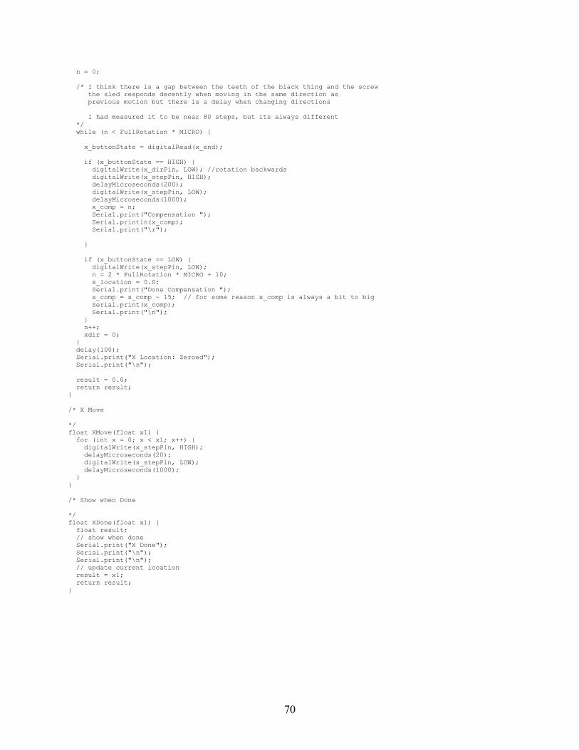
70
n = 0; /* I think there is a gap between the teeth of the black thing and the screw the sled responds decently when moving in the same direction as previous motion but there is a delay when changing directions I had measured it to be near 80 steps, but its always different */ while (n < FullRotation * MICRO) { x_buttonState = digitalRead(x_end); if (x_buttonState == HIGH) { digitalWrite(x_dirPin, LOW); //rotation backwards digitalWrite(x_stepPin, HIGH); delayMicroseconds(200); digitalWrite(x_stepPin, LOW); delayMicroseconds(1000); x_comp = n; Serial.print("Compensation "); Serial.println(x_comp); Serial.print("\r"); } if (x_buttonState == LOW) { digitalWrite(x_stepPin, LOW); n = 2 * FullRotation * MICRO + 10; x_location = 0.0; Serial.print("Done Compensation "); x_comp = x_comp - 15; // for some reason x_comp is always a bit to big Serial.print(x_comp); Serial.print("\n"); } n++; xdir = 0; } delay(100); Serial.print("X Location: Zeroed"); Serial.print("\n"); result = 0.0; return result; } /* X Move */ float XMove(float x1) { for (int x = 0; x < x1; x++) { digitalWrite(x_stepPin, HIGH); delayMicroseconds(20); digitalWrite(x_stepPin, LOW); delayMicroseconds(1000); } } /* Show when Done */ float XDone(float x1) { float result; // show when done Serial.print("X Done"); Serial.print("\n"); Serial.print("\n"); // update current location result = x1; return result; }

71
Focus.h
//Laser Diode Focusing #define SEL1 12 #define SEL2 7 #define LS_PWR 8 #define LS_LNS 10 #define FE A3 void FocusLaser();
72
Focus.cpp #include "focus.h" #include "Arduino.h" //function to get the focus position void FocusLaser() { int sensorMin = 1023; // minimum sensor value int sensorMax = 0; // maximum sensor value int x = 1; for (int i = 0; i > -1; i = i + x) //move lens up and down once { int fe = analogRead(FE); OCR2A = i; if (i == 255) x = -1; //switch direction at peak https://www.arduino.cc/en/reference/for delay(5); // record the maximum sensor value see https://www.arduino.cc/en/Tutorial/Calibration if (fe > sensorMax) { sensorMax = fe; } // record the minimum sensor value if (fe < sensorMin) { sensorMin = fe; } } //if there isn't a max over a certain value generate an error //determine the amplitue of the S-curve int amp = sensorMax - sensorMin; //calculate a upper and lower acceptable postion for the laser to be focused see http://www.diyouware.com/img/image037.jpg int fe_focus_position_pos = 506 + (amp / 16); int fe_focus_position_neg = 506 - (amp / 16); int motor_pwm_position_value = 0; delay(1000); x = 1; int i = 1; do //do while loop, moves lens top to bottom while the fe signal is not equal to the upper or lower focus limit(fe_focus_position_pos/neg) { int fe = analogRead(FE); OCR2A = i; //sets lens at top i = i + x; if (i % 255 == 1) i = 1; //if its at the bottom it resets to top, ie. if i is divisible exactly by 255 it means the lens is at the bottom motor_pwm_position_value = i; delayMicroseconds(500); // } while (analogRead(FE) > fe_focus_position_pos || analogRead(FE) < fe_focus_position_neg || analogRead(FE) < 510 || analogRead(FE) > 502); } while (analogRead(FE) != fe_focus_position_pos && analogRead(FE) != fe_focus_position_neg); // more consistent but takes longer OCR2A = motor_pwm_position_value; // OCR2A = 50; //130 neutral height } MotorControl.h
// Copyright Pololu Corporation. For more information, see http://www.pololu.com/ /*! \file AMIS30543.h * * This is the main header file for the AMIS30543 library, a library for * controllering the AMIS-30543 micro-stepping stepper motor driver. * * For an overview of the features of this library, see * * https://github.com/pololu/fastgpio-arduino * * That is the main repository for this library, * */ #pragma once #include <stdint.h>

73
#include <Arduino.h> #include <SPI.h> /*! This class provides low-level functions for reading and writing from the SPI * interface of an AMIS-30543 micro-stepping stepper motor driver. * * Most users should use the AMIS30543 class, which provides a higher-level * interface, instead of this class. */ class AMIS30543SPI { public: /*! Configures this object to use the specified pin as a slave select pin. * You must use a slave select pin; the AMIS-30543 requires it. */ void init(uint8_t slaveSelectPin) { ssPin = slaveSelectPin; digitalWrite(ssPin, HIGH); pinMode(ssPin, OUTPUT); } /*! Reads the register at the given address and returns its raw value. */ uint8_t readReg(uint8_t address) { selectChip(); transfer(address & 0b11111); uint8_t dataOut = transfer(0); deselectChip(); return dataOut; } /*! Writes the specified value to a register. */ void writeReg(uint8_t address, uint8_t value) { selectChip(); transfer(0x80 | (address & 0b11111)); transfer(value); // The CS line must go high after writing for the value to actually take // effect. deselectChip(); } private: SPISettings settings = SPISettings(9600, MSBFIRST, SPI_MODE0); uint8_t transfer(uint8_t value) { return SPI.transfer(value); } void selectChip() { digitalWrite(ssPin, LOW); SPI.beginTransaction(settings); } void deselectChip() { digitalWrite(ssPin, HIGH); SPI.endTransaction(); // The CS high time is specified as 2.5 us in the AMIS-30543 datasheet. delayMicroseconds(3); } uint8_t ssPin; }; /*! This class provides high-level functions for controlling an AMIS-30543 * micro-stepping motor driver. * * It provides access to all the features of the AMIS-30543 SPI interface * except the watchdog timer. */ class AMIS30543 { public: /*! The default constructor. */ AMIS30543() { wr = cr0 = cr1 = cr2 = cr3 = 0; }

74
/*! Possible arguments to setStepMode(). */ enum stepMode { MicroStep128 = 128, MicroStep64 = 64, MicroStep32 = 32, MicroStep16 = 16, MicroStep8 = 8, MicroStep4 = 4, MicroStep2 = 2, MicroStep1 = 1, CompensatedHalf = MicroStep2, CompensatedFullTwoPhaseOn = MicroStep1, CompensatedFullOnePhaseOn = 200, UncompensatedHalf = 201, UncompensatedFull = 202, }; /*! Bitmasks for the return value of readNonLatchedStatusFlags(). */ enum nonLatchedStatusFlag { OPENY = (1 << 2), OPENX = (1 << 3), WD = (1 << 4), CPFAIL = (1 << 5), TW = (1 << 6), }; /*! Bitmasks for the return value of readLatchedStatusFlagsAndClear(). */ enum latchedStatusFlag { OVCXNB = (1 << 3), OVCXNT = (1 << 4), OVCXPB = (1 << 5), OVCXPT = (1 << 6), TSD = (1 << 10), OVCYNB = (1 << 11), OVCYNT = (1 << 12), OVCYPB = (1 << 13), OVCYPT = (1 << 14), }; /*! Addresses of control and status registers. */ enum regAddr { WR = 0x0, CR0 = 0x1, CR1 = 0x2, CR2 = 0x3, CR3 = 0x9, SR0 = 0x4, SR1 = 0x5, SR2 = 0x6, SR3 = 0x7, SR4 = 0xA, }; /*! Configures this object to use the specified pin as a slave select pin. * You must use a slave select pin; the AMIS-30543 requires it. */ void init(uint8_t slaveSelectPin) { driver.init(slaveSelectPin); } /*! Changes all of the driver's settings back to their default values. * * It is good to call this near the beginning of your program to ensure that * There are no settings left over from an earlier time that might affect the * operation of the driver. */ void resetSettings() { wr = cr0 = cr1 = cr2 = cr3 = 0; applySettings(); } /*! Reads back all the SPI control registers from the device and * verifies that they are equal to the cached copies stored in this class. * * This can be used to verify that the driver is powered on and has not lost * them due to a power failure. However this function will probably return * true if the driver is not powered and all of the cached settings are the * default values. Therefore, we only recommend calling this after you have * changed at least one of the settings from its default value, for example

75
* by calling enableDriver(). * * @return 1 if the settings from the device match the cached copies, 0 if * they do not. */ bool verifySettings() { return driver.readReg(WR) == wr && driver.readReg(CR0) == cr0 && driver.readReg(CR1) == cr1 && driver.readReg(CR2) == cr2 && driver.readReg(CR3) == cr3; } /*! Re-writes the cached settings stored in this class to the device. * * You should not normally need to call this function because settings are * written to the device whenever they are changed. However, if * verifySettings() returns false (due to a power interruption, for * instance), then you could use applySettings to get the device's settings * back into the desired state. */ void applySettings() { // Because of power interruption considerations, the register that // contains the MOTEN bit (CR2) must be written first, and whenever we // write to it we should also write to all the other registers. // CR2 is written first, because it contains the MOTEN bit, and there is // a risk that there might be a power interruption to the driver right // before CR2 is written. This could result in the motor being enabled // with incorrect settings. Also, whenever we do write to CR2, we want to // also write the other registers to make sure they are in the correct state. driver.writeReg(CR2, cr2); writeWR(); writeCR0(); writeCR1(); writeCR3(); } /*! Sets the MOTEN bit to 1, enabling the driver. * * Please read the note about this function in README.md. */ void enableDriver() { cr2 |= 0b10000000; applySettings(); } /*! Sets the MOTEN bit to 0, disabling the driver. * * Please read the note about this function in README.md. */ void disableDriver() { cr2 &= ~0b10000000; applySettings(); } /*! Sets the per-coil current limit equal to the highest available setting * that is less than the given current, in units of milliamps. * * Refer to Table 13 of the AMIS 30543 datasheet to see which current limits * are available. */ void setCurrentMilliamps(uint16_t current) { // This comes from Table 13 of the AMIS-30543 datasheet. uint8_t code = 0; %uncomment if (current >= 3000) ( code = 0b11001; ) else if (current >= 2845) ( code = 0b11000; ) else if (current >= 2700) ( code = 0b10111; ) else if (current >= 2440) ( code = 0b10110; ) else if (current >= 2240) ( code = 0b10101; ) else if (current >= 2070) ( code = 0b10100; ) else if (current >= 1850) { code = 0b10011; ) else if (current >= 1695) ( code = 0b10010; ) else if (current >= 1520) ( code = 0b10001; ) else if (current >= 1405) ( code = 0b10000; ) else if (current >= 1260) ( code = 0b01111; ) else if (current >= 1150) ( code = 0b01110; ) else if (current >= 1060) ( code = 0b01101; ) else if (current >= 955) ( code = 0b01100; ) else if (current >= 870) ( code = 0b01011; ) else if (current >= 780) ( code = 0b01010; )

76
else if (current >= 715) ( code = 0b01001; ) else if (current >= 640) ( code = 0b01000; ) else if (current >= 585) ( code = 0b00111; ) else if (current >= 540) ( code = 0b00110; ) else if (current >= 485) ( code = 0b00101; ) else if (current >= 445) ( code = 0b00100; ) else if (current >= 395) ( code = 0b00011; ) else if (current >= 355) ( code = 0b00010; ) else if (current >= 245) ( code = 0b00001; ) cr0 = (cr0 & 0b11100000) | code; writeCR0(); } /*! Reads the current microstepping position, which is a number between 0 * and 511. * * The different positions and their corresponding coil values are listed in * Table 9 of the AMIS 30543 datasheet. * * The lower two bits of this return value might be inaccurate if the step * pin is being toggled while this function runs (e.g. from an interrupt or * a PWM signal). * * Our tests indicated that the return value of this function might be wrong * if you read it within 25 microseconds of commanding the driver to take a * step. Therefore we recommend delaying for at least 100 microseconds after * taking a step and before calling this function. */ uint16_t readPosition() { uint8_t sr3 = readStatusReg(SR3); uint8_t sr4 = readStatusReg(SR4); return ((uint16_t)sr3 << 2) | (sr4 & 3); } /*! Sets the value of the DIRCTRL configuration bit. * * Allowed values are 0 or 1. * * You can use this command to control the direction of the stepper motor * and simply leave the DIR pin disconnected. */ void setDirection(bool value) { if (value) { cr1 |= 0x80; } else { cr1 &= ~0x80; } writeCR1(); } /*! Returns the cached value of the DIRCTRL configuration bit. * * This does not perform any SPI communication with the driver. */ bool getDirection() { return cr1 >> 7 & 1; } /*! Configures the driver to have the specified stepping mode. * * This affects many things about the performance of the motor, including * how much the output moves for each step taken and how much current flows * through the coils in each stepping position. * * If an invalid stepping mode is passed to this function, then it selects * 1/32 micro-step, which is the driver's default. */ void setStepMode(uint8_t mode) { // Pick 1/32 micro-step by default. uint8_t esm = 0b000; uint8_t sm = 0b000; // The order of these cases matches the order in Table 12 of the // AMIS-30543 datasheet. switch(mode) { case MicroStep32: sm = 0b000; break; case MicroStep16: sm = 0b001; break; case MicroStep8: sm = 0b010; break;

77
case MicroStep4: sm = 0b011; break; case CompensatedHalf: sm = 0b100; break; /* a.k.a. MicroStep2 */ case UncompensatedHalf: sm = 0b101; break; case UncompensatedFull: sm = 0b110; break; case MicroStep128: esm = 0b001; break; case MicroStep64: esm = 0b010; break; case CompensatedFullTwoPhaseOn: esm = 0b011; break; /* a.k.a. MicroStep 1 */ case CompensatedFullOnePhaseOn: esm = 0b100; break; } cr0 = (cr0 & ~0b11100000) | (sm << 5); cr3 = (cr3 & ~0b111) | esm; writeCR0(); writeCR3(); } /*! Sets the SLP bit 1, enabling sleep mode. * * According to the AMIS-30543 datasheet, the motor supply voltage must be * at least 9 V before entering sleep mode. * * You can call sleepStop() to disable sleep mode. * * Please read the note about this function in README.md. */ void sleep() { cr2 |= (1 << 6); applySettings(); } /*! Sets the SLP bit 0, disabling sleep mode. * * Please read the note about this function in README.md. */ void sleepStop() { cr2 &= ~(1 << 6); applySettings(); } /*! Sets the value of the NXTP configuration bit to 0, which means that new * steps are triggered by a rising edge on the NXT/STEP pin. This is the * default behavior. */ void stepOnRisingEdge() { cr1 &= ~0b01000000; writeCR1(); } /*! Sets the value of the NXTP configuration bit to 1, which means that new * steps are triggered by a falling edge on the NXT/STEP pin. */ void stepOnFallingEdge() { cr1 |= 0b01000000; writeCR1(); } /*! Sets the PWMF bit to 1, which doubles the PWM frequency (45.6 kHz) .*/ void setPwmFrequencyDouble() { cr1 |= (1 << 3); writeCR1(); } /*! Clears the PWMF bit, which sets the PWM frequency to its default value * (22.8 kHz). */ void setPwmFrequencyDefault() { cr1 &= ~(1 << 3); writeCR1(); } /*! Sets the PWMJ bit, which enables artificial jittering in the PWM signal * used to control the current to each coil. */ void setPwmJitterOn() { cr1 |= (1 << 2); writeCR1(); } /*! Clears the PWMJ bit, which disables artificial jittering in the PWM * signal used to control the current to each coil. This is the default * setting. */ void setPwmJitterOff()
78
{ cr1 &= ~(1 << 2); writeCR1(); } /*! This sets the EMC[1:0] bits, which determine how long it takes the PWM * signal to rise or fall. Valid values are 0 through 3. Higher values * correspond to longer rise and fall times. **/ void setPwmSlope(uint8_t emc) { cr1 = (cr1 & ~0b11) | (emc & 0b11); writeCR1(); } /*! Clears the SLAG bit, which configures the signal on SLA pin to have a * gain of 0.5 (the default). * * Please read the note about this function in README.md. */ void setSlaGainDefault() { cr2 &= ~(1 << 5); applySettings(); } /*! Sets the SLAG bit to 1, which configures the signal on SLA pin to have a * gain of 0.25 (half of the default). * * Please read the note about this function in README.md. */ void setSlaGainHalf() { cr2 |= (1 << 5); applySettings(); } /*! Set the SLAT bit to 0 (the default), which disables transparency on the * SLA pin. See the AMIS-30543 datasheet for more information. * * Please read the note about this function in README.md. */ void setSlaTransparencyOff() { cr2 &= ~(1 << 4); applySettings(); } /*! Sets the SLAT bit to 1, which enables transparency on the SLA pin. * See the AMIS-30543 datasheet for more information. * * Please read the note about this function in README.md. */ void setSlaTransparencyOn() { cr2 |= (1 << 4); applySettings(); } /*! Reads the status flags from registers SR0. These flags are not latched, * which means they will be cleared as soon as the condition causing them is * no longer detected. See the AMIS-30543 datasheet for more information. * * This function returns the raw value of SR0, with the parity bit set to 0. * You can simply compare the return value to 0 to see if any of the status * flags are set, or you can use the logical AND operator (`&`) and the * #nonLatchedStatusFlag enum to check individual flags. * * ~~~~(.cpp) * uint16_t flags = stepper.readNonLatchedStatusFlags(); * if (flags) * { * // At least one flag is set. * * if (flags & AMIS30543::OPENX) * { * // Thermal shutdown flag is set. * } * * } * ~~~~ */ uint16_t readNonLatchedStatusFlags() { return readStatusReg(SR0); } /*! Reads the latched status flags from registers SR1 and SR2. They are

79
* cleared as a side effect. * * The return value is a 16-bit unsigned integer that has one bit for each * status flag. You can simply compare the return value to 0 to see if any * of the status flags are set, or you can use the logical and operator (`&`) * and the #latchedStatusFlag enum to check individual flags. * * WARNING: Calling this function clears the latched error bits in SR1 and * SR2, which might allow the motor driver outputs to reactivate. The * AMIS-30543 datasheet says "successive reading the SPI Status Registers 1 * and 2 in case of a short circuit condition, may lead to damage to the * drivers". */ uint16_t readLatchedStatusFlagsAndClear() { uint8_t sr1 = readStatusReg(SR1); uint8_t sr2 = readStatusReg(SR2); return (sr2 << 8) | sr1; } protected: uint8_t wr, cr0, cr1, cr2, cr3; /*! Reads a status register and returns the lower 7 bits (the parity bit is * set to 0 in the return value). */ uint8_t readStatusReg(uint8_t address) { // Mask off the parity bit. // (Later we might add code here to check the parity // bit and record errors.) return driver.readReg(address) & 0x7F; } /*! Writes the cached value of the WR register to the device. */ void writeWR() { driver.writeReg(WR, wr); } /*! Writes the cached value of the CR0 register to the device. */ void writeCR0() { driver.writeReg(CR0, cr0); } /*! Writes the cached value of the CR1 register to the device. */ void writeCR1() { driver.writeReg(CR1, cr1); } /*! Writes the cached value of the CR3 register to the device. */ void writeCR3() { driver.writeReg(CR3, cr3); } public: /*! This object handles all the communication with the AMIS-30543. It is * only marked as public for the purpose of testing this library; you should * not use it in your code. */ AMIS30543SPI driver; };

80
Appendix E: How to Collect and Analyze Data
Blu-ray Data Collection Process
1. Wire it up. Function generator to lock in and IR. Photodiode to lock-in. Lock-in to
computer. 2. Turn on everything. There are 6 things to turn on including the Arduino
a. Power supply b. Lock in c. Photodiode power supply d. Photodiode e. Function generator f. Arduino
3. Set up function generator a. Hi level: 3.3V, low level: 2V
4. Open Matlab data acquisition program: J:\groups\munroresearc\Data\Blu-Ray Project\SR830_data_acquisition
5. Unlock lock in so it is referencing function generator, not itself 6. Name file in frequency box, it saves to where the data acquisition file is saved
a. Image of file name box

81
Curve Fitting Data with Fitmain.m
1. Open fitmain located in J:\groups\munroresearc\Programs\MATLAB\Christ_codes 2. This will open:
a. Data should be in the following format: frequency (Hz), phase delay (degrees)
1. Enter initial guess for thermal
diffusivity, ie (1e-6 200 0), the last two
numbers are just mathematical
constants
2. Press button then select file
containing phase
3. Press to change to log scale
4. Press then type in name of fitting
function
5. Calculates results of model
6. Press to begin the fitting process

82
3. After it runs, the best fit parameters box will list the thermal diffusivity as the first parameter