The Design and Experimental Analysis of an Air

Source Heat Pump for Extreme Cold Weather

Operation

by

Tom Mackintosh, B.A.Sc., Mechanical Engineering

University of Ottawa

A thesis submitted to the Faculty of Graduate Studies and Postdoctoral Affairs in

partial fulfillment of the requirements for the degree of

Master of Applied Science

in

Mechanical Engineering

Ottawa - Carleton Institute for Mechanical and Aerospace Engineering

Carleton University

Ottawa, Ontario

January, 2016

c© 2016

Tom Mackintosh

Abstract

Heat pumps offer the potential for significant energy savings in residential applica-

tions if they are implemented properly. Currently, air source heat pumps have limited

performance at outdoor temperatures below -5C and most are unable to operate at

outdoor temperatures below -15C. This means less efficient backup heating systems

are necessary to meet heating requirements which has impeded widespread use of this

technology in Canadian climates.

This research evaluates one method of increasing the performance of an air sourced

heat pump to extend its operating range and eliminate the need for a backup heating

system.

A study was conducted using the Engineering Equation Solver software package

to identify the performance improvements that are attainable with variations of a two

stage heat pump cycle. An experimental apparatus was constructed to compare the

performance of the best performing variation - a two stage economized cycle - to that

of a traditional single stage heat pump.

The two stage economized heat pump had a measured coefficient of performance

of 1.45 when it was operated at an outdoor temperature of -31C making it an energy

efficient option for most Canadian climates. In addition, the heating capacity of the

system was increased by a factor of 2.5 when compared to the single stage system.

ii

Contents

Abstract ii

List of Tables vi

List of Figures vii

1 Introduction 11.1 Motivation . . . . . . . . . . . . . . . . . . . . . . . . . . . . . . . . . 11.2 Literature Review . . . . . . . . . . . . . . . . . . . . . . . . . . . . . 6

1.2.1 Environmental Regulations . . . . . . . . . . . . . . . . . . . . 71.2.2 Cascade Cycle . . . . . . . . . . . . . . . . . . . . . . . . . . . 71.2.3 Multi-stage Cycles . . . . . . . . . . . . . . . . . . . . . . . . 81.2.4 Auto-cascade Cycle . . . . . . . . . . . . . . . . . . . . . . . . 111.2.5 Carbon Dioxide Cycle . . . . . . . . . . . . . . . . . . . . . . 121.2.6 Hydrocarbon Refrigerants . . . . . . . . . . . . . . . . . . . . 131.2.7 Compressor Technology . . . . . . . . . . . . . . . . . . . . . 14

1.3 Research Objectives . . . . . . . . . . . . . . . . . . . . . . . . . . . . 151.4 Thesis Outline . . . . . . . . . . . . . . . . . . . . . . . . . . . . . . . 16

2 Modelling 172.1 Refrigerant . . . . . . . . . . . . . . . . . . . . . . . . . . . . . . . . 172.2 Model Components . . . . . . . . . . . . . . . . . . . . . . . . . . . . 18

2.2.1 Compressors . . . . . . . . . . . . . . . . . . . . . . . . . . . . 182.2.2 Heat Exchangers . . . . . . . . . . . . . . . . . . . . . . . . . 22

2.2.2.1 Condenser . . . . . . . . . . . . . . . . . . . . . . . . 222.2.2.2 Evaporator . . . . . . . . . . . . . . . . . . . . . . . 23

2.2.3 Expansion Valves . . . . . . . . . . . . . . . . . . . . . . . . . 242.3 Single Stage Cycle . . . . . . . . . . . . . . . . . . . . . . . . . . . . 252.4 Two Stage Cascade Cycle . . . . . . . . . . . . . . . . . . . . . . . . 262.5 Two Stage Flash Separation Cycle . . . . . . . . . . . . . . . . . . . . 28

2.5.1 Flash Separation Tank . . . . . . . . . . . . . . . . . . . . . . 292.5.2 Interstage Mixing . . . . . . . . . . . . . . . . . . . . . . . . . 292.5.3 Two Stage Flash Separation Model Solution . . . . . . . . . . 30

2.6 Two Stage Economized Cycle . . . . . . . . . . . . . . . . . . . . . . 302.6.1 Economizer . . . . . . . . . . . . . . . . . . . . . . . . . . . . 312.6.2 Two Stage Economized Model Solution . . . . . . . . . . . . . 32

2.7 Modelling Results . . . . . . . . . . . . . . . . . . . . . . . . . . . . . 322.7.1 Effect of Intermediate Pressure on Performance . . . . . . . . 33

2.8 Closing Remarks . . . . . . . . . . . . . . . . . . . . . . . . . . . . . 34

iii

3 Experiment Design and Construction 353.1 Apparatus . . . . . . . . . . . . . . . . . . . . . . . . . . . . . . . . . 35

3.1.1 Refrigerant Path . . . . . . . . . . . . . . . . . . . . . . . . . 363.2 Cycle Modifications . . . . . . . . . . . . . . . . . . . . . . . . . . . . 37

3.2.1 Low Pressure Compressor . . . . . . . . . . . . . . . . . . . . 373.2.2 System Piping and Auxiliary Components . . . . . . . . . . . 393.2.3 Modified Refrigerant Path . . . . . . . . . . . . . . . . . . . . 40

3.3 Control . . . . . . . . . . . . . . . . . . . . . . . . . . . . . . . . . . 413.3.1 System Controller . . . . . . . . . . . . . . . . . . . . . . . . . 423.3.2 LP Compressor . . . . . . . . . . . . . . . . . . . . . . . . . . 423.3.3 HP Compressor . . . . . . . . . . . . . . . . . . . . . . . . . . 433.3.4 Expansion Valves . . . . . . . . . . . . . . . . . . . . . . . . . 453.3.5 Solenoids and 4-Way Valve . . . . . . . . . . . . . . . . . . . . 453.3.6 Fans . . . . . . . . . . . . . . . . . . . . . . . . . . . . . . . . 453.3.7 Auxiliary Systems . . . . . . . . . . . . . . . . . . . . . . . . . 463.3.8 Programming . . . . . . . . . . . . . . . . . . . . . . . . . . . 473.3.9 Instrumentation . . . . . . . . . . . . . . . . . . . . . . . . . . 48

3.3.9.1 Critical Measurements . . . . . . . . . . . . . . . . . 493.3.9.2 Support Instrumentation . . . . . . . . . . . . . . . . 52

3.4 Closing Remarks . . . . . . . . . . . . . . . . . . . . . . . . . . . . . 53

4 Uncertainty 554.1 Bias Error . . . . . . . . . . . . . . . . . . . . . . . . . . . . . . . . . 554.2 Precision Error . . . . . . . . . . . . . . . . . . . . . . . . . . . . . . 564.3 Overall Uncertainty . . . . . . . . . . . . . . . . . . . . . . . . . . . . 564.4 Heating Capacity Uncertainty . . . . . . . . . . . . . . . . . . . . . . 574.5 COP Uncertainty . . . . . . . . . . . . . . . . . . . . . . . . . . . . . 614.6 Calibration and Uncertainty Reduction . . . . . . . . . . . . . . . . . 63

4.6.1 Calibration . . . . . . . . . . . . . . . . . . . . . . . . . . . . 644.6.2 Bias Quantification . . . . . . . . . . . . . . . . . . . . . . . . 654.6.3 Verification . . . . . . . . . . . . . . . . . . . . . . . . . . . . 68

5 Test Plan and System Operation 715.1 System Operation . . . . . . . . . . . . . . . . . . . . . . . . . . . . . 72

5.1.1 System Preheating . . . . . . . . . . . . . . . . . . . . . . . . 735.1.2 Startup Procedure . . . . . . . . . . . . . . . . . . . . . . . . 74

5.1.2.1 Super-heat Control Algorithm . . . . . . . . . . . . . 745.1.3 Economized Operation . . . . . . . . . . . . . . . . . . . . . . 755.1.4 Intermediate Pressure . . . . . . . . . . . . . . . . . . . . . . 755.1.5 LP Compressor . . . . . . . . . . . . . . . . . . . . . . . . . . 775.1.6 Steady State Operation . . . . . . . . . . . . . . . . . . . . . . 775.1.7 Defrost Cycle . . . . . . . . . . . . . . . . . . . . . . . . . . . 78

5.2 Closing Remarks . . . . . . . . . . . . . . . . . . . . . . . . . . . . . 78

iv

6 Results and Discussion 796.1 Heating Capacity . . . . . . . . . . . . . . . . . . . . . . . . . . . . . 806.2 COP . . . . . . . . . . . . . . . . . . . . . . . . . . . . . . . . . . . . 816.3 Comparison With Modelling Results . . . . . . . . . . . . . . . . . . 816.4 Real-World Implications . . . . . . . . . . . . . . . . . . . . . . . . . 84

6.4.1 Optimized COP . . . . . . . . . . . . . . . . . . . . . . . . . . 856.4.2 Variable Heating Capacity . . . . . . . . . . . . . . . . . . . . 85

6.5 Closing Remarks . . . . . . . . . . . . . . . . . . . . . . . . . . . . . 86

7 Conclusions and Recommendations 877.1 Conclusions and Contributions . . . . . . . . . . . . . . . . . . . . . . 877.2 Recommendations for Future Work . . . . . . . . . . . . . . . . . . . 88

References 90

A EES Models 93

B FPGA 104B.1 FPGA Function . . . . . . . . . . . . . . . . . . . . . . . . . . . . . . 104

C Expansion Valve Control 106C.1 Expansion Valves . . . . . . . . . . . . . . . . . . . . . . . . . . . . . 106

D Fans 110D.1 Fans . . . . . . . . . . . . . . . . . . . . . . . . . . . . . . . . . . . . 110

E Software 112E.1 Architecture . . . . . . . . . . . . . . . . . . . . . . . . . . . . . . . . 112

E.1.1 Desktop PC . . . . . . . . . . . . . . . . . . . . . . . . . . . . 112E.1.2 Main Controller . . . . . . . . . . . . . . . . . . . . . . . . . . 112

E.1.2.1 FPGA . . . . . . . . . . . . . . . . . . . . . . . . . . 113E.1.3 Hydronics Controller . . . . . . . . . . . . . . . . . . . . . . . 114E.1.4 PA-4000 . . . . . . . . . . . . . . . . . . . . . . . . . . . . . . 114

F Uncertainty 115F.1 PA-4000 Additional Terms . . . . . . . . . . . . . . . . . . . . . . . . 115F.2 Uncertainty . . . . . . . . . . . . . . . . . . . . . . . . . . . . . . . . 116

G Super-heat Algorithm 118G.1 Super-heat Defined . . . . . . . . . . . . . . . . . . . . . . . . . . . . 118G.2 PID Algorithm . . . . . . . . . . . . . . . . . . . . . . . . . . . . . . 119

H Data 122H.1 Data Points . . . . . . . . . . . . . . . . . . . . . . . . . . . . . . . . 122

v

List of Tables

1.1 Months Included in Heating Season Data . . . . . . . . . . . . . . . . 31.2 Backup Heating System Operating Time . . . . . . . . . . . . . . . . 6

2.1 Compressor Isentropic Efficiency Coefficients for Equation 2.6 . . . . 21

3.1 Motor Torque Compatibility Study . . . . . . . . . . . . . . . . . . . 393.2 Controlled Components . . . . . . . . . . . . . . . . . . . . . . . . . . 433.3 NI cRIO-9074 Modules . . . . . . . . . . . . . . . . . . . . . . . . . . 433.4 Denso Motor Parameters . . . . . . . . . . . . . . . . . . . . . . . . . 443.5 Mitsubishi Motor Parameters . . . . . . . . . . . . . . . . . . . . . . 44

4.1 Heating Capacity Component Bias Errors for Example Case . . . . . 584.2 Heat Transfer Fluid Properties and Associated Bias Errors for Example

Case . . . . . . . . . . . . . . . . . . . . . . . . . . . . . . . . . . . . 594.3 Temperature Differential Bias Error . . . . . . . . . . . . . . . . . . . 594.4 Heating Capacity Sensitivity Factors and Total Bias Error . . . . . . 604.5 Heating Capacity Total Uncertainty for Example Case . . . . . . . . 604.6 COP Bias Error Calculation for Example Case . . . . . . . . . . . . . 624.7 COP Precision Error and Total Uncertainty for Example Case . . . . 624.8 Measured Temperature Differential Bias Error [B∆T ] . . . . . . . . . 684.9 Measured Temperature Bias Error During Verification . . . . . . . . . 70

5.1 Test Matrix 50C Supply Temperature . . . . . . . . . . . . . . . . . 715.2 Modified Test Matrix 40C Supply Temperature . . . . . . . . . . . . 72

C.1 Expansion Valve Stepping Sequence . . . . . . . . . . . . . . . . . . . 106

D.1 Outdoor Unit Fan Pinout . . . . . . . . . . . . . . . . . . . . . . . . 110

F.1 PA-4000 Bias Error Terms . . . . . . . . . . . . . . . . . . . . . . . . 115

G.1 Measured Open Loop Response Parameters . . . . . . . . . . . . . . 120

vi

List of Figures

1.1 Ottawa Heating Season Climate Data (September - May) . . . . . . . 41.2 Edmonton Heating Season Climate Data (September - June) . . . . . 41.3 Cambridge Bay Heating Season Climate Data (Full Year) . . . . . . . 51.4 Resolute Heating Season Climate Data (Full Year) . . . . . . . . . . . 51.5 Two Stage Inter-cooled Cycle Diagram . . . . . . . . . . . . . . . . . 91.6 Two Stage Auto-cascade Cycle Diagram . . . . . . . . . . . . . . . . 12

2.1 Compressor Control Volume . . . . . . . . . . . . . . . . . . . . . . . 182.2 Range of Isentropic Efficiencies Calculated using Equation 2.6 . . . . 212.3 Condenser Heat Transfer Diagram . . . . . . . . . . . . . . . . . . . . 232.4 Evaporator Heat Transfer Diagram . . . . . . . . . . . . . . . . . . . 242.5 Single Stage Cycle Diagram . . . . . . . . . . . . . . . . . . . . . . . 252.6 Single Stage TS Diagram (Tambient = 0C, Tsupply = 50C) . . . . . . . 262.7 Two Stage Cascade Cycle Diagram . . . . . . . . . . . . . . . . . . . 272.8 Intermediate Heat Exchanger Heat Transfer Diagram . . . . . . . . . 272.9 Two Stage Flash Separation Cycle Diagram . . . . . . . . . . . . . . 282.10 Interstage Mixing Control Volume . . . . . . . . . . . . . . . . . . . . 292.11 Two Stage Flash Separation Cycle Diagram . . . . . . . . . . . . . . 312.12 Modelling Results . . . . . . . . . . . . . . . . . . . . . . . . . . . . . 332.13 Effect of Intermediate Pressure on Two Stage Economized Heat Pump

COP. . . . . . . . . . . . . . . . . . . . . . . . . . . . . . . . . . . . . 34

3.1 Mitsubishi Zuba Heat Pump Cycle (Heating Mode) . . . . . . . . . . 363.2 Two Stage Economized Heat Pump Cycle (Heating Mode) . . . . . . 403.3 Modified Heat Pump . . . . . . . . . . . . . . . . . . . . . . . . . . . 423.4 Hydronic System Schematic . . . . . . . . . . . . . . . . . . . . . . . 463.5 Hydronic System . . . . . . . . . . . . . . . . . . . . . . . . . . . . . 473.6 Refrigerated Container . . . . . . . . . . . . . . . . . . . . . . . . . . 483.7 Power Measurement Patch Box . . . . . . . . . . . . . . . . . . . . . 513.8 Surface Mounted RTD Section View . . . . . . . . . . . . . . . . . . 533.9 Installation Location of Support Instrumentation . . . . . . . . . . . 54

4.1 Measured Temperature vs. SPRT Reading . . . . . . . . . . . . . . . 664.2 Time Series of Long Term Temperature Difference Data . . . . . . . . 674.3 Verification Data 30C . . . . . . . . . . . . . . . . . . . . . . . . . . 694.4 Verification Data 50C . . . . . . . . . . . . . . . . . . . . . . . . . . 70

5.1 System Operating Schematics . . . . . . . . . . . . . . . . . . . . . . 735.2 Two Stage Compression Process . . . . . . . . . . . . . . . . . . . . . 765.3 Intermediate Pressure vs. LP Compressor Speed . . . . . . . . . . . . 77

6.1 Measured Heating Capacity During Experimental Investigation . . . . 806.2 Measured COP During Experimental Investigation . . . . . . . . . . 826.3 Comparison Between Measured and Modelled COP . . . . . . . . . . 83

vii

A.1 Single Stage Cycle EES Model Page. 1 . . . . . . . . . . . . . . . . . 94A.2 Single Stage Cycle EES Model Page. 2 . . . . . . . . . . . . . . . . . 95A.3 Two Stage Cascade Cycle EES Model Page. 1 . . . . . . . . . . . . . 96A.4 Two Stage Cascade Cycle EES Model Page. 2 . . . . . . . . . . . . . 97A.5 Two Stage Cascade Cycle EES Model Page. 3 . . . . . . . . . . . . . 97A.6 Two Stage Flash Separation Cycle EES Model Page. 1 . . . . . . . . 98A.7 Two Stage Flash Separation Cycle EES Model Page. 2 . . . . . . . . 99A.8 Two Stage Flash Separation Cycle EES Model Page. 3 . . . . . . . . 100A.9 Two Stage Economized Cycle EES Model Page. 1 . . . . . . . . . . . 101A.10 Two Stage Economized Cycle EES Model Page. 2 . . . . . . . . . . . 102A.11 Two Stage Economized Cycle EES Model Page. 3 . . . . . . . . . . . 103

B.1 Architecture of FPGA Building Block . . . . . . . . . . . . . . . . . . 105

C.1 Expansion Valve FPGA Software Operation . . . . . . . . . . . . . . 107C.2 Expansion Valve Current Driving Circuit (Showing One Internal Dar-

lington) . . . . . . . . . . . . . . . . . . . . . . . . . . . . . . . . . . 108

D.1 DC Rectifier Circuit . . . . . . . . . . . . . . . . . . . . . . . . . . . 111

E.1 System Software Architecture . . . . . . . . . . . . . . . . . . . . . . 113E.2 System Graphical User Interface . . . . . . . . . . . . . . . . . . . . . 114

F.1 Details of Uncertainty Analysis - 1 . . . . . . . . . . . . . . . . . . . 116F.2 Details of Uncertainty Analysis - 2 . . . . . . . . . . . . . . . . . . . 117

G.1 Super-heat Open Loop Step Response . . . . . . . . . . . . . . . . . . 120

H.1 Data Point Legend . . . . . . . . . . . . . . . . . . . . . . . . . . . . 123H.2 Averaged Data From Analysis . . . . . . . . . . . . . . . . . . . . . . 124

viii

Nomenclature

Acronyms

COP Coefficient of performance

cRIO Compact RIO

DAQ Data acquisition system

EES Engineering Equation Solver

FPGA Field programmable gate array

HP High pressure

HCFC Hydrochloroflourocarbon

HFC Hydroflourocarbon

IC Integrated circuit

LP Low pressure

NI National Instruments

PID Proportional-Integral-Derivative

PWM Pulse width modulation

RTD Resistance temperature detector

SPRT Secondary platinum resistance thermometer

SJ SJ series variable speed drive

SCPI Standard commands for programmable instruments

VFD Variable frequency drive

WJ WJ series variable speed drive

Symbols

X Arithmetic mean

Bi Bias error for a given component in the measurement system

Bj Bias error for the quantity produced by the measurement system

V Bulk fluid velocity

ρ Density

ix

η Efficiency

E Energy within control volume

h Enthalpy

S Entropy

ε Error

g Force due to gravity

Cp Heat capacity at constant pressure

Q Heat rate

QH Heating capacity

Z Height

EV Induced voltage

B Magnetic field flux density

m Mass flow rate

N Number of instantaneous derived measurement quantities

pherr Phase error

PF Power factor

P Power

S Precision error

Pr Pressure ratio

P Pressure

a, b, c Regression coefficients

ω Rotational speed

θj Sensitivity factor used during uncertainty analysis

S Standard deviation

ts Student T statistic

Σ Summation

∆T Temperature differential

x

T Temperature

t Time

Tq Torque

BT Total bias error for a derived quantity

U Total uncertainty margin for an average derived quantity

~V Velocity

V– Volume

W Work rate

Unit Prefix

c Centi

k Kilo

m Milli

Subscripts

acc Accuracy

C.V. Control volume

elec Electrical

i Entering C.V.

εT Error of temperature measurement

e Exiting C.V.

eS Exiting state assuming isentropic process

rms Root mean square

suction State at compressor inlet

discharge State at compressor outlet

1, 2, 3, ... State point location reference

T Temperature

Units

A Amps

xi

C Degrees Celsius

Ω Electrical resistance

Hz Frequency (Hertz)

g Grams

J Joules

L Litres

m Metres

min Minutes

rpm Revolutions per minute

rev Revolutions

s Seconds

Vac Voltage - alternating current

Vdc Voltage - direct current

V Voltage

W Watts

xii

Chapter 1

Introduction

1.1 Motivation

The Canadian heating season is an extreme case of climate variability. Southern

Canada experiences heat and humidity during the summer while being subject to

moderately cold average temperatures with occasional periods of extremely cold tem-

peratures in the winter. The northern regions of Canada experience low to moderate

temperatures in summer and extremely cold temperatures in the winter. Although

the required heating capacity varies throughout the year in each of these climates,

building codes require the heating system to be sized to provide adequate heat during

the lowest temperatures experienced in their respective regions [1].

Heating systems can be categorized into two groups. The first group includes

systems whose performance is reasonably independent of outdoor temperature, and

can be scaled to handle the worst case loading expected for the house. This cate-

gory includes gas furnaces, boilers, and systems which operate within the home, and

therefore their operation is only dependent on the internal temperature of the home.

The second group includes systems whose performance and heating capacity are

negatively affected by the ambient temperature outside the home, including air source

heat pumps. For this type of system there is a more complicated solution to assure

that adequate heating capacity is available during the extreme low temperatures.

Historically, heat pump systems have been sized to accommodate the load at a specific

outdoor temperature, below which a backup system is used. To meet the requirements

of the building code, the backup system is sized for the worst case loading and the

1

heat pump is used when the ambient temperature permits. Backup systems are

usually resistive heating elements because houses that use heat pumps typically do

not have primary energy sources other than electricity. Resistive elements are a low

cost addition to the original heat pump system, however they are expensive to operate.

To understand the issue of using a resistive heating element as a main heating

source, the coefficient of performance (COP) for a heating system is calculated using

its general definition in Equation 1.1.

COPHeating =HeatingCapacity

EnergyInput(1.1)

The COP gives a metric for comparing heating systems. In the most basic study,

the COP of a heat pump system is a function of the temperatures of the heat source

and the heat sink that it operates between. In home heating systems, the source is

the ambient air and the sink is the house. Because the house temperature is relatively

stable, the COP is directly proportional to the temperature of the ambient air and

can range from less than 1 to greater than 5. A resistive heating element has a COP

of 1 as it is 100% efficient at converting electrical energy into thermal energy. This is

the foundation of the argument that there is no benefit to using a heat pump when

its COP is below 1, as a resistive heating element would have better performance.

Most heat pumps available today automatically switch over to their backup system

at a preset temperature. This may be an attempt to conserve energy or a result of

mechanical limitations. Unfortunately, in many cases, backup systems take over well

before the heat pump COP drops below 1.

The lower operating range for a heat pump greatly depends on its design and

varies from one manufacturer to another. A typical lower operating point for current

state-of-the-art systems is in the range of -5C to -15C. Below this temperature, the

system cannot or does not operate and the backup system is used. This presents the

2

question: What percentage of the time are temperatures lower than this encountered

in Canadian cities?

In order to quantify this, Environment Canada climate data [2] from four Canadian

cities were evaluated for the years 2007 to 2011. The study included two reasonably

populated non-maritime cities - Ottawa and Edmonton - and two extreme northern

cities - Cambridge Bay and Resolute.

For this study, an hour that required heating was defined as an hour during the

heating season when the outdoor ambient temperature was below 15C. This was done

to neglect hours when the outdoor temperature was above 15C as these were assumed

to not require heating. For each city, the heating season was defined as the months

of the year when the average daily temperature was less than 15C. This means that

hourly outdoor temperatures below 15C that occurred outside of the heating season

were neglected. For example, cool summer nights do not require heating. Table 1.1

states the months that were considered to be the heating seasons for each city.

Table 1.1: Months Included in Heating Season Data

City Heating Season

Ottawa September to MayEdmonton September to JuneCambridge Bay Full YearResolute Full Year

Figures 1.1, 1.2, 1.3 and 1.4 plot temperature against the percentage of hours

when the outdoor temperature was at or below that temperature. For example, in

Figure 1.1, which displays Ottawa temperature data, the outdoor temperature was

at or below 12C for 90% of the hours that required heating.

Figures 1.1, 1.2, 1.3 and 1.4 indicate that in each of the cities studied, assuming

heat pump shutoff temperatures of -5C or -15C, there would have been a substantial

amount of time when a backup heating system was required if a typical heat pump

3

-35

-30

-25

-20

-15

-10

-5

0

5

10

15

0 10 20 30 40 50 60 70 80 90 100

Tem

pera

ture

(°C)

Percentage of Hours Below Temperature (15°C Reference)

Ottawa (2007 - 2011)

Figure 1.1: Ottawa Heating Season Climate Data (September - May)

-40

-35

-30

-25

-20

-15

-10

-5

0

5

10

15

0 10 20 30 40 50 60 70 80 90 100

Tem

pera

ture

(°C)

Percentage of Hours Below Temperature (15°C Reference)

Edmonton (2007 - 2011)

Figure 1.2: Edmonton Heating Season Climate Data (September -June)

4

-50

-45

-40

-35

-30

-25

-20

-15

-10

-5

0

5

10

15

0 10 20 30 40 50 60 70 80 90 100

Tem

pera

ture

(°C)

Percentage of Hours Below Temperature (15°C Reference)

Cambridge Bay (2007 - 2011)

Figure 1.3: Cambridge Bay Heating Season Climate Data (Full Year)

-50

-45

-40

-35

-30

-25

-20

-15

-10

-5

0

5

10

15

0 10 20 30 40 50 60 70 80 90 100

Tem

pera

ture

(°C)

Percentage of Hours Below Temperature (15°C Reference)

Resolute (2007 - 2011)

Figure 1.4: Resolute Heating Season Climate Data (Full Year)

5

was used to heat a home. Table 1.2 shows the amount of time during the heating

season when the backup system would have been required to operate in each city.

This data is presented as the percentage of hours that required heating during the

heating season when the ambient temperature was at or below the heat pump shutoff

temperature and also as the number of hours during the heating season when the

ambient temperature was at or below the heat pump shutoff temperature.

Table 1.2: Backup Heating System Operating Time

Operating Limitation of Heat Pump-5C -15C

Climate % Below Hours % Below Hours

Ottawa 27% 1763 6% 391Edmonton 30% 2182 12% 873Cambridge Bay 60% 5256 47% 4117Resolute 65% 5694 49% 4292

These results indicate that there would have been significant benefit from using

an air source heat pump that is capable of operating at reduced temperatures while

maintaining both a reasonable COP and sufficient capacity to heat the home. To

determine the current state of research in this area, a literature review was conducted.

1.2 Literature Review

In the past decade, there has been an effort to increase the performance of heat pump

cycles. This was motivated by regulations which restrict the use of certain refrigerants

and the public interest in reducing energy consumption.

6

1.2.1 Environmental Regulations

The regulations under the Montreal Protocol and the amendments from the United

Nations Environmental Programme currently dictate the phasing out of hydrochlo-

rofluorocarbons (HCFCs) by 2030 [3]. This has driven a wave of innovation in creating

new refrigerants and developing new cycles that better suit these refrigerants. Hy-

drofluorocarbon (HFC) refrigerants are one option, although there are indications

that these refrigerants will also be phased out in the future [4]. As a result of these

phase outs, it is important to be reasonably confident that refrigerants being studied

will be available in the future.

In addition, there have been studies focused on increasing the performance and

operating range of heat pump cycles in general.

1.2.2 Cascade Cycle

The simplest approach to improving heat pump cycles focuses on extending the op-

erating range using a cascade cycle. This arrangement uses two or more single stage

vapour compression cycles in series1, which allows the low temperature cycle to use a

refrigerant which is better suited to lower temperatures, while also splitting the work

between multiple compression processes which allows a higher total pressure ratio to

be achieved than is possible with a single compressor.

Parekh et al. [5] studied a cascade cycle which used R-507a and R-23 refrigerants.

The study included steady state modelling with the intention of extending the range

of the system to operate at lower temperatures. The study showed that the system

was capable of operating at ambient temperatures below -50C, although the COP

at these temperatures was expected to be on the order of 0.8. The authors assumed

compressor isentropic efficiencies of 80%.

1The Single Stage Cycle and Cascade Cycle schematics are included in Chapter 2.

7

Bhattacharyya et al. [6] performed a similar study on a two stage cascade heat

pump using N2O and CO2 as refrigerants. The cycle they studied used additional

internal heat exchangers that super-heated the refrigerant at the compressor inlets

by drawing heat from the liquid refrigerant after it was condensed. The researchers

performed optimization on parameters which included: intermediate heat exchanger

overlap temperature, intermediate temperature and heat exchanger effectiveness. The

authors’ report predicted COPs of 2.5 at an ambient temperature of -35C and 2 at

an ambient temperature of -65C. They did not discuss operation at temperatures

above this range.

1.2.3 Multi-stage Cycles

Another approach to increasing heat pump performance is to use multiple compression

stages with a single refrigerant. This may include the use of additional performance

improving features related to cycle arrangement.

Bertsch et al. performed an extensive study of two stage air source heat pumps.

Their initial investigation focused on determining which cycle would be best suited

to residential applications where the supplied heating temperature was 50C and the

ambient temperature was as low as -30C [7]. This study compared the relative

performance of a two stage inter-cooled cycle, a two stage economized cycle2, and

a cascade cycle to a standard single stage cycle. The two stage inter-cooled cycle

functioned by removing heat from the refrigerant after the first compression stage

via an additional heat exchanger. Depending on its temperature, the heat was either

used for heating or dumped as waste heat. A schematic of the two stage inter-cooled

cycle is shown in Figure 1.5.

2The two stage economized cycle schematic is included in Chapter 2.

8

Low Pressure Compressor

High Pressure Compressor

Condenser

Evaporator

Expansion Valve Inter-cooler

Figure 1.5: Two Stage Inter-cooled Cycle Diagram

They concluded that each of the studied cycles had their own strengths and weak-

nesses and the best cycle would depend on the operating environment of the end

user.

A second study conducted by Bertsch et al. included building an experimental

system based on their previous work [8]. The two stage economized cycle was chosen

as the base for this study. Their experimental apparatus was designed to operate in

both a two stage and a traditional single stage configuration to allow for comparison.

This study showed that their two stage cycle was able to achieve a COP of 2.1 at an

ambient temperature of -30C. The authors also observed an increase in the amount

of deliverable heat by a factor of roughly 2 when compared to single stage operation.

When the authors compared the experimental results with their original modelling

study, they found the modelled performance was approximately 20% higher than the

measured performance. They concluded this was reasonable based on the simplicity

of the model. The authors also concluded that oil management is very important

in multiple stage cycles that are operated at low temperatures. Their system used

9

a manual approach to maintain the oil distribution between the compressors before

each test run.

The work of Bertsch et al. was continued by Caskey [9] and Menzi [10] who

each performed a study using an improved version of the cycle that Bertsch et al.

worked with. This version of the cycle included a low pressure compressor bypass

system which allowed the system to operate as a single stage cycle at warmer ambient

temperatures.

Caskey’s work focused on a TRNSYS study which compared the performance of

the two stage economized air source heat pump to a gas furnace in a military barracks

in Indiana using an updated version of the original model. The study showed that a

yearly COP of 3.67 for the system could be expected with an operating cost savings

of 25% and a reduction in CO2 emissions of 30%.

Menzi’s study included a larger set of cases within a TRNSYS simulation of the

military barracks in Indiana. This study compared the performance of three different

systems: a standard gas furnace, a single stage air source heat pump, and the two

stage economized air source heat pump. The single stage system used an electrical

backup heater to help with cold weather operation and was used for comparison in

two studies. The first study used the original buildings, and the second study used

the buildings with upgraded insulation and air tightness. The two stage system also

used these two scenarios, as well as a case where the upgraded building also used

ambient heating or cooling when it was available. This allowed the outdoor ambient

air to heat or cool the interior directly if the outdoor temperature allowed. There

were additional cases added for the two stage system which included a latent heat

storage system that was regenerated daily with outdoor air, a night time setback

program in the thermostat, and a case where the thermostat could switch between

heating and cooling based on outdoor temperature. Altogether, eight cases were used

and the results presented for each were primary energy consumption, heating/cooling

10

delivered, CO2 emissions, cost, and relative energy usage compared to a gas furnace.

Menzi concluded that for this installation, both the single stage and the two stage

system operated similarly, as the cold weather operation was mainly above -20C

in this region. It was his recommendation that the time below -15C be studied to

determine whether or not the two stage system was beneficial.

Wang et al studied the benefits of using a single compressor with an intermediate

injection port [11]. An intermediate injection port allows refrigerant to be injected

into the compressor part way through the compression process. This essentially splits

the compression process into two stages within a single machine. This study included

an experimental investigation of both the economized and the flash tank method for

vapour injection3. These cycles were similar to those studied by Bertsch et al., except

for the use of a single compressor with a vapour injection port. The study used

R-410a as the refrigerant and the vapour injected mass was varied from 0 kg/s to

the maximum amount possible for each cycle. It was shown that the capacity of the

system could be increased during both heating and cooling, while the COP showed

appreciable gains during the heating season only. Wang also concluded that both

approaches had different advantages. He states that the flash tank was slightly more

efficient, although it required a more advanced control strategy.

1.2.4 Auto-cascade Cycle

There has also been work done with the auto-cascade cycle. This cycle uses a sin-

gle compressor with a mixture of refrigerants. The operating principle separates

refrigerants by taking advantage of their different saturation temperatures for a given

pressure. The mixture of vapour refrigerants is compressed, after which they are sepa-

rated one by one in different condensing steps. After a fluid condenses, it is expanded

and used as a heat sink to condense the next fluid. Any number of fluids can be

3The flash tank cycle schematic is included in Chapter 2.

11

used to obtain the required temperature reduction. A schematic of a two-refrigerant

auto-cascade cycle is shown in Figure 1.6.

Compressor

Condenser(Refrigerant 1)

Evaporator

Expansion Valve

Phase Separation

Tank

Condenser (Refrigerant 2)

Expansion Valve

Figure 1.6: Two Stage Auto-cascade Cycle Diagram

Du et al. [12] studied the auto-cascade cycle as a means for ultra-low temperature

refrigeration in the range of -60C. The authors conducted an experimental study

which used a mixture of R-134a and R-23. They successfully operated their system

with an evaporator temperature of -60C. They concluded that this cycle could per-

form with a good COP. However, the additional heat exchangers and phase separators

required would all need to be optimized as they increase energy losses when compared

to a more standard cycle.

1.2.5 Carbon Dioxide Cycle

Carbon dioxide (CO2) is being used more often in small scale systems. Carbon

dioxide is an interesting fluid in that it has a global warming potential of 1 as it is the

reference gas for this parameter. It also has a critical point of 31.1C which allows it

to be used in a trans-critical cycle within air source heat pumps. Trans-critical cycles

12

replace the condenser with a gas cooler, which reduces entropy generation during the

heat transfer process.

Austin performed an extensive review of trans-critical carbon dioxide heat pumps

in 2011 [13], which highlights the benefits of such systems. Austin notes that the

main disadvantage of using carbon dioxide as a refrigerant is its extremely high pres-

sure requirements (≥11 MPa) which present challenges in system design, but he also

states that carbon dioxide systems are smaller than comparable systems due to the

high volumetric heating capacity of CO2. Austin states that in earlier studies there

were many conflicting results which showed poor performance. This conflict has been

attributed to the vastly varying properties of CO2 near its critical temperature. The

author states that if the changes in viscosity and heat capacity are modelled accu-

rately, there is a substantial improvement in the predicted performance. Austin also

presents market data showing that trans-critical CO2 heat pumps are available in

Japan from various manufacturers sold under the name Eco-Cute. As of 2009, there

have been 2 million of these units sold. Austin also notes that Coca Cola has stated

that its vending machines will be replaced with trans-critical CO2 units by 2015.

1.2.6 Hydrocarbon Refrigerants

Recent studies have also investigated using hydrocarbons as refrigerants. Westphalen

converted a military environmental control unit to operate on propylene rather than

R-407c and studied the resulting change in performance [14]. The system previously

had a heating capacity of 15.9 kW. The author determined that a 12% increase in

output and a 10% increase in the COP were attainable by simply switching refriger-

ants. The author also determined that this translates to a reduction in the required

heat exchanger surface area of 8.5% if the original heating requirement was retained.

Lastly, the author investigated the potential explosion and fire hazards that could

result from a leak of refrigerant. It was determined that due to the small mass of

13

refrigerant, there would only be a flammable mixture present for a short period of

time. However, in the design used, no ignition sources were present within the system

and it was not considered a safety hazard.

1.2.7 Compressor Technology

Residential heat pump compressors are typically positive displacement machines.

This has been driven by air conditioning expertise which has a much greater market

share than residential heat pumps in North America. These compressors are typically

either piston-based or scroll-based, with the current trend favouring scroll compressors

for their simplicity, relative performance, and low-noise operation. Larger commercial

scale heat pumps also use screw and centrifugal compressors although this technology

is starting to emerge in studies at smaller scales as well. Typical isentropic efficiencies

of residential-sized positive displacement compressors are in the range of 40% to 70%

[15].

There have been recent studies on the possibility of using turbo-machinery de-

rived compressors for residential heat pumps. Schiffman et al. [16][17] conducted a

study on the feasibility of using a small centrifugal compressor in a residential-sized

heat pump. Their main goal was to exploit the wide operating range of centrifugal

machines in terms of mass flow rates and pressure ratios as a way to increase the heat

pump efficiency. They also note the benefits of oil-free operation, reduced compres-

sor size, and a potential increase in isentropic efficiency associated with centrifugal

machines. The study included a modelling investigation of the compressor, using the

assumption of one-dimensional internal flow, followed by the design of a prototype

and an experimental investigation. The system was intended to produce hot water

at a rate of 12 kW at a temperature of 60C and operated with an evaporator tem-

perature of -12C. The study showed that the predicted results were lower than what

was measured during the experiment by approximately 5%, the compressor was able

14

to operate over a wide flow rate range of 27 g/s to 55 g/s, the isentropic efficiency

was above 70% for most of the operating range, and the compressor could reach a

maximum isentropic efficiency of 80%. This was all achieved using a compressor with

an exducer diameter of 20 mm which presents an incredibly small footprint when

compared to a similar capacity scroll compressor.

1.3 Research Objectives

The previous section outlines the work which has been conducted related to residen-

tial air source heat pumps. With the exception of the work done by Bertsch et al.

[7][8], and Du et al. [12], this work has been limited to either modelling or experi-

mentation at ambient temperatures above -15C. This demonstrates a need to extend

the operating performance of air source heat pumps to temperatures below -30C

through experimentation. This thesis will outline the work that was done in this area

through the following research objectives:

1. Conduct an investigation of different heat pump cycles using Engineering Equa-

tion Solver (EES) to determine the best heat pump candidate for the Canadian

climate. The cycles that will be considered are:

• Single stage

• Two stage cascade

• Two stage economized

• Two stage flash separation

2. Design and build an experimental prototype of the best performing cycle as

determined by Objective 1.

3. Characterize the cold climate performance of the prototype through experimen-

tal investigation.

15

At the time of this research, a modern air source cold climate heat pump was made

available which allowed the experimental prototype to be constructed by modifying

a market ready system. The system was designed to operate on R-410a and as such,

the modelling study was limited to this refrigerant.

1.4 Thesis Outline

With the research objectives defined, the remainder of this thesis is organized as

follows:

• Chapter 2 will describe the modelling study that was conducted to determine

which cycle should be constructed for the experimental work.

• Chapter 3 will describe the construction of the experimental prototype and the

instrumentation that was used to characterize its performance.

• Chapter 4 will outline the work done to characterize the uncertainty of the

measured results.

• Chapter 5 will outline the test plan that was followed to characterize the per-

formance of the system. The operation of the prototype heat pump will also be

described here.

• Chapter 6 will outline the results of the experimental investigation and discuss

their implications.

• Chapter 7 will present a conclusion of the work that is discussed in this thesis.

16

Chapter 2

Modelling

This chapter outlines the work that was done during the modelling study. The study

was intended to show the performance of the two stage cycles relative to a single stage

cycle and also identify which cycle should be studied further during the experimental

phase of this work. A simple thermodynamic model for each cycle was developed

using the software package Engineering Equation Solver (EES) which is developed

by F-Chart. EES is designed to solve coupled algebraic and differential equations. It

also includes built-in thermodynamic state equations for many fluids. This software

is extremely powerful for these types of studies as it reduces the time required to

formulate the problem and eliminates the need to manually input fluid property

information. The cycle models that are outlined in this chapter have been included

in Appendix A.

2.1 Refrigerant

As outlined in Section 1.3, the modelling study was limited to the refrigerant R-

410a which is a 50/50 mass percentage blend of R-32 and R-125. EES calculates the

fluid properties for R-410a using the pseudo-pure fluid equations of state that were

developed by Lemmon [18]. These equations are able to predict the properties of

R-410a with an accuracy of 0.1% when compared to experimental data.

17

2.2 Model Components

The models for each cycle were constructed using component models which created

links between the state points of the cycles. The component models are described in

the following sections.

2.2.1 Compressors

Each compression process was modelled using the approach that is outlined in this

section. Figure 2.1 shows the control volume that was used to model a compressor.

푚

푚

푊

Figure 2.1: Compressor Control Volume

The compression process was modelled by simplifying the First Law of Thermo-

dynamics for a control volume which is shown in Equation 2.1.

dEC.V.dt

= QC.V. − WC.V. + Σmi

(hi +

1

2~Vi

2+ gZi

)− Σme

(he +

1

2~Ve

2+ gZe

)(2.1)

where dEC.V.

dtis the rate of change in energy within the control volume, QC.V. is the

rate at which heat is added to the control volume, −WC.V. is the rate at which work

is extracted from the control volume, Σmi and Σme are the sum of the mass flows

that enter and exit the control volume respectively, h is the enthalpy of a flow as it

18

crosses the boundary of the control volume, 12~V 2 is the kinetic energy of a flow as it

crosses the boundary of the control volume, and gZ is the potential energy of a flow

as it crosses the boundary of the control volume.

Equation 2.1 was simplified using the following assumptions:

1. The process is steady state.

2. There is no heat loss from the system.

3. The change in kinetic energy is negligible.

4. The change in potential energy is negligible.

5. There is a single inlet and outlet in the control volume.

Equation 2.1 is shown below in its full form with the cancelled terms crossed out.

>

1dEC.V.dt

= *2

QC.V. −WC.V.+5

Σ mi

(hi+

1

2

3~Vi

2+>

4gZi

)−

5Σ me

(he+

1

2

3~Ve

2+

*4gZe

)

Lastly, conservation of mass for a system operating at steady state dictates that

mi = me = m. The simplified form of Equation 2.1 is shown in Equation 2.2.

WC.V. = m(hi − he) (2.2)

Equation 2.2 shows that the work consumed by the compressor is directly related

the mass flow of refrigerant flowing through it and the difference in the enthalpies

of the refrigerant between its inlet and outlet. For this work the inlet pressure and

temperature were known while only the outlet pressure was known. To determine the

outlet state, the isentropic efficiency was used as defined in Equation 2.3

ηIsentropic =WIsentropicCompression

WRealCompression

(2.3)

19

where, WIsentropicCompression is the work required for an isentropic compression process

and WRealCompression is the work required for a real compression process that includes

the mechanical and electrical losses. This relation allows the outlet state of the com-

pression process to be estimated using isentropic efficiencies which are representative

of a real machine. For a given mass flow rate and by substitution of Equation 2.2,

Equation 2.3 becomes:

ηIsentropic =hi − heShi − he

(2.4)

where heS is the outlet enthalpy for the isentropic process and he is the outlet enthalpy

for the real process. Equation 2.4 was rearranged to allow the outlet state to be solved

directly. The final form of the compressor model is shown in Equation 2.5.

he = hi +heS − hiηIsentropic

(2.5)

This approach requires the isentropic efficiency to be defined in order to solve the

outlet conditions. For this work, the isentropic efficiency was determined by fitting

a second order polynomial to the manufacturer’s performance data of a Copeland

ZP36K5E-PFJ R-410a scroll compressor. Copeland publishes performance data for

all of their compressors online [15]. The ZPE36K5E-PFJ was chosen as it is represen-

tative of a high performance modern scroll compressor that was designed for operation

with R-410a. The equation that was fitted to the data is shown in Equation 2.6.

ηIsentropic = a+ b ∗ Pr + c ∗ P 2r (2.6)

where Pr is the pressure ratio across the compressor. The coefficients were regressed

using condenser data for 51C as this was representative of expected testing condi-

tions. The coefficients are shown in table 2.1.

Figure 2.2 plots the range of isentropic efficiencies that result from Equation 2.6.

20

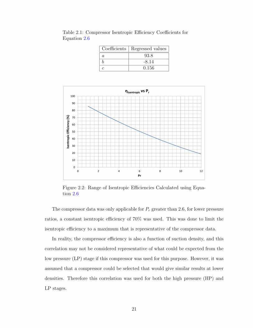
Table 2.1: Compressor Isentropic Efficiency Coefficients forEquation 2.6

Coefficients Regressed values

a 93.8b -8.14c 0.156

0

10

20

30

40

50

60

70

80

90

100

0 2 4 6 8 10 12

Isen

trop

ic E

ffici

ency

(%)

Pr

ηIsentropic vs Pr

Figure 2.2: Range of Isentropic Efficiencies Calculated using Equa-tion 2.6

The compressor data was only applicable for Pr greater than 2.6, for lower pressure

ratios, a constant isentropic efficiency of 70% was used. This was done to limit the

isentropic efficiency to a maximum that is representative of the compressor data.

In reality, the compressor efficiency is also a function of suction density, and this

correlation may not be considered representative of what could be expected from the

low pressure (LP) stage if this compressor was used for this purpose. However, it was

assumed that a compressor could be selected that would give similar results at lower

densities. Therefore this correlation was used for both the high pressure (HP) and

LP stages.

21

2.2.2 Heat Exchangers

The heat exchangers were not modelled based on actual components. Instead, it was

assumed that a heat exchanger with similar performance could be designed for each

cycle. To account for the heat exchange process, the temperature of the ambient

air and the indoor air were assumed to be constant throughout the heat exchanger.

This was considered to be a reasonable assumption because these heat exchangers are

typically the tube and fin type where the air stream flows perpendicular to the refrig-

erant. To ensure the heat transfer process was possible, the temperature difference

between the refrigerant and the heat source or the heat sink at the pinch point was

assumed to be 3C. This value was used as it agrees with the experimental results

that were published by Bertsch et al. [8].

2.2.2.1 Condenser

The condensing process was assumed to provide a fixed amount of 8.3C of sub-cooling

at the refrigerant outlet. This means that the refrigerant exited the condenser at 8.3C

below its saturation temperature. This value was chosen because it corresponds to the

value used by Copeland during their compressor performance testing. Defining the

amount of sub-cooling at the outlet of the condenser, dictated the saturation temper-

ature, and therefore the pressure of the condenser. Figure 2.3 shows the temperature

of the refrigerant as it passes through the condenser.

To model this process, the saturation temperature was fixed using Equation 2.7.

TsatCond= Tsupply + Tpinch + Tsub−cool (2.7)

where TsatCondis the saturation temperature of the refrigerant in the condenser, Tsupply

is the temperature of the air supplied to the house, Tpinch is the temperature differ-

ential required to drive the heat transfer process, and Tsub−cool is the desired amount

22

T

x

Air

Mixed-phase region

De-super-heat

Sub-cooling

Pinch Point

Refrigerant

Figure 2.3: Condenser Heat Transfer Diagram.

of sub-cooling at the condenser outlet. For this work, a value of 50C was used for

Tsupply. This value was chosen as it was the value used by Bertsch et al.[7] during

their work. This temperature is representative of what is required for a forced air

heating system.

2.2.2.2 Evaporator

The evaporation process was assumed to provide a fixed amount of 11.1C of super-

heat at the refrigerant outlet. This means that the refrigerant exited the evaporator

at 11.1C above its saturation temperature. This value corresponds to the amount of

super-heat that was used by Copeland during their compressor performance testing.

Defining the amount of super-heat at the outlet of the evaporator, dictated the sat-

uration temperature, and therefore the pressure of the evaporator. Figure 2.4 shows

the temperature of the refrigerant as it passed through the evaporator.

To model this process, the saturation temperature was fixed using Equation 2.8.

23

T

x

Air

Mixed-phase regionSuper-heating

Pinch Point

Refrigerant

Figure 2.4: Evaporator Heat Transfer Diagram.

TsatEvap= Tambient − Tpinch − Tsuper−heat (2.8)

where, TsatEvapis the saturation temperature of the evaporator, Tambient is the tem-

perature of the ambient air, and Tsuper−heat is the desired amount of super-heat at the

evaporator outlet.

2.2.3 Expansion Valves

The expansion valves were modelled using the same assumptions outlined in Section

2.2.1, with the additional assumption that no work is done on the system during the

expansion process. This further reduced Equation 2.2 to give Equation 2.9, which

was used to determine the outlet state of the expansion valve.

*

0WC.V. = m(hi − he)

24

he = hi (2.9)

2.3 Single Stage Cycle

Compressor

Condenser

Evaporator

Expansion Valve

Figure 2.5: Single Stage Cycle Diagram

The single stage cycle diagram, shown in Figure 2.5, was modelled by linking the

previously mentioned component models. The supply temperature was set to 50C

and the ambient temperature was set for the desired case. The model was then solved

on a per-unit mass basis for the COP and the process was repeated to populate the

ambient temperature range of -20C to 20C in 10C increments. This range was

chosen because it spans the operating range of currently available cold climate heat

pumps. Figure 2.6 shows the Temperature-Entropy diagram for the single stage cycle

when operated at an ambient temperature of 0C.

25

File:SingleStageTS.EES 2015-10-26 11:03:52 Page 1EES Ver. 9.660: #3243: For use only by Tom Mackintosh Natural, Resources Canada

0.50 0.75 1.00 1.25 1.50 1.75 2.00 2.25 2.50-100

-50

0

50

100

150

200

s [kJ/kg-K]

T [°

C]

3500 kPa

1700 kPa

710 kPa

230 kPa 0.2 0.4 0.6 0.8

0.0

019

0.0

09

0.0

19

0.0

43

0.0

94

0.2

m3/

kg

R410A

Figure 2.6: Single Stage TS Diagram (Tambient = 0C, Tsupply =50C)

2.4 Two Stage Cascade Cycle

The two stage cascade cycle diagram, shown in Figure 2.7, operated using two separate

single stage cycles that were connected via an intermediate heat exchanger which

acted both as the LP stage’s condenser and the HP stage’s evaporator.

This new heat exchanger was also modelled by assuming a 3C temperature dif-

ference at its pinch point. This heat exchanger was assumed to be a counterflow type.

Figure 2.8 shows the temperature of the refrigerant flows as they pass through the

intermediate heat exchanger.

To model this process, the HP stage’s evaporator saturation temperature was set

to the intermediate saturation temperature and the LP stage’s condenser saturation

temperature was calculated using Equation 2.10.

TSatLPCond= Tintermediate + Tpinch + Tsub−cool (2.10)

26

LP Compressor

HP Compressor

Condenser

Evaporator

HP Expansion Valve

LP Expansion Valve

Intermediate HX

Figure 2.7: Two Stage Cascade Cycle Diagram

T

x

LP Condenser

HP EvaporatorPinch Point

Figure 2.8: Intermediate Heat Exchanger Heat Transfer Diagram

27

where, TSatLPCondis the saturation temperature of the LP stage’s condenser, and

Tintermediate is the intermediate saturation temperature.

The two stage cascade cycle was solved by setting the supply temperature to

50C and setting the ambient temperature for the desired case. The intermediate

saturation temperature was than varied in 1C increments from Tambient to Tsupply to

locate the operating point that resulted in the highest COP. The process was repeated

to populate the ambient temperature range of -40C to 0C in 10C increments.

2.5 Two Stage Flash Separation Cycle

The two stage flash separation cycle diagram, shown in Figure 2.9, uses two expansion

valves which split the expansion process. After the first expansion, the flash separation

tank separates the two phase fluid into its liquid and gaseous states. The liquid is

further expanded by the second expansion valve while the vapour phase is injected

between the two compression processes.

LP Compressor

HP Compressor

Condenser

Evaporator

Expansion Valve

ExpansionValve

Flash Separation Tank

Figure 2.9: Two Stage Flash Separation Cycle Diagram

28

To model this cycle, the flash tank and mixing process were modelled using the

following approaches.

2.5.1 Flash Separation Tank

The flash separation tank was modelled using the assumptions that (a) during steady

state operation the liquid level in the tank is constant, and (b) the liquid and vapour

exiting flows are single phase flows. Therefore, the quality of the two phase fluid

entering the tank determines the division of vapour and liquid mass flows that must

exit the tank to maintain the liquid level. The pressure of the flash separation tank

was assumed to be the saturation pressure that corresponded to the intermediate

temperature used for the given case.

2.5.2 Interstage Mixing

The interstage mixing process was modelled using the control volume shown in Figure

2.10.

푚 ,

푚 ,

푚

Figure 2.10: Interstage Mixing Control Volume

Equation 2.1 was reduced using the following assumptions:

1. The process is steady state.

2. There is no heat loss from the system.

29

3. The change in kinetic energy is negligible.

4. The change in potential energy is negligible.

5. There is no work done on the system.

Equation 2.1 is shown below in its full form with the cancelled terms crossed out.

>

1dEC.V.dt

= *2

QC.V. −*

5WC.V. +Σmi

(hi+

1

2

3~Vi

2+>

4gZi

)−Σme

(he+

1

2

3~Ve

2+

*4gZe

)

Lastly, conservation of mass for a system operating at steady state dictates that

Σmi = Σme, or specific to this case mi,1 + mi,2 = me. The resulting form of Equation

2.1 was rearranged to allow the outlet state to be solved directly. The final form of

the interstage mixing model is shown in Equation 2.11.

he =mi,1 ∗ he,1 + mi,2 ∗ hi,2

mi,1 + mi,2

(2.11)

2.5.3 Two Stage Flash Separation Model Solution

The two stage flash separation model was solved by setting the supply temperature

to 50C and setting the ambient temperature for the desired case. The intermediate

saturation temperature was than varied in 1C increments from Tambient to Tsupply to

locate the operating point that resulted in the highest COP.

2.6 Two Stage Economized Cycle

The two stage economized cycle diagram, shown in Figure 2.11, used two expansion

valves. The second expansion valve was used to directly control the interstage in-

jection mass flow rate. An additional heat exchanger, or economizer, was used to

30

increase the sub-cooling of the main refrigerant flow, as well as increase the vapour

mass fraction of the injection stream.

LP Compressor

HP Compressor

Condenser

Evaporator

Economizer

Expansion Valve

Expansion Valve

Figure 2.11: Two Stage Flash Separation Cycle Diagram

The method described in Section 2.5.2 was used to solve the interstage mixing

process.

2.6.1 Economizer

The economizer was modelled as an ideal heat transfer process. The outlet states

were calculated by solving the energy balance that is shown in Equation 2.12.

m1 ∗ (h1 − h2) = m2 ∗ (h4 − h3) (2.12)

Where, m1 is the mass flow of the main refrigerant stream with states 1 and 2

referring to the inlet and outlet respectively, and m2 is the mass flow of the injected

stream with states 3 and 4 referring to the inlet and outlet conditions respectively.

31

2.6.2 Two Stage Economized Model Solution

The two stage economized model was solved by setting the supply temperature to

50C and setting the ambient temperature for the desired case. At each ambient tem-

perature, the model was solved for all possible intermediate saturation temperatures

between the ambient and supply temperatures. The mass flow rate of injection was

than varied at each intermediate temperature by varying the injection ratio from 0

to 0.8, as defined in Equation 2.13.

Xinjection =minjection

mcondenser

(2.13)

where, minjection is the mass flow of the injection stream and mcondenser is the mass

flow through the condenser. The optimal COP was then chosen for each ambient

temperature.

2.7 Modelling Results

The resulting COPs for each cycle were plotted for comparison across the operating

range. These results are shown in Figure 2.12.

The results indicate that a substantial improvement in the COP of a heat pump

can be achieved when two compressors are used. This is evident at all ambient tem-

peratures that were studied. There is also a strong indication that the operating

range of a heat pump can be extended to lower ambient temperatures than are cur-

rently being achieved by residential systems. Lastly, a COP of greater than 1.5 can

be maintained at temperatures below -40C which could eliminate the need for a

backup heating system and reduce the energy consumption of these systems. Each of

the two stage cycles shows similar performance with the cascade cycle being slightly

lower performing than the flash separation and economized cycles. This is a result

32

0.00

0.50

1.00

1.50

2.00

2.50

3.00

3.50

4.00

-50.00 -40.00 -30.00 -20.00 -10.00 0.00 10.00 20.00

COP

Ambient Temperature [C]

Heating COP vs. Ambient Temperature of Various Heat Pump Cycles

(R-410a)

Single Stage 2 Stage Cascade 2 Stage Economized 2 Stage Flash Separation

Figure 2.12: Modelling Results

of the additional work that is required to provide the temperature difference in the

intermediate heat exchanger.

2.7.1 Effect of Intermediate Pressure on Performance

The optimal intermediate pressures for the two stage cycles were determined through

trial and error. To illustrate the effect this parameter has on the performance of the

cycles, the two stage economized model was used to plot the COP of the cycle against

intermediate saturation pressure shown in Figure 2.13.

This indicates that there is an optimal intermediate pressure that corresponds to

the maximum COP of the heat pump for each ambient temperature. The results

show three regimes of performance. Below 350 kPa, the isentropic efficiency of the

LP compressor is fixed at 70%, as the pressure ratio of this compressor is less than

2.6. Between 350 kPa and 950 kPa, both compressors are operating with pressure

ratios greater than 2.6 and the isentropic efficiency is calculated using Equation 2.6.

Above 950 kPa, the isentropic efficiency of the HP compressor is fixed at 70%, as the

33

0.00

0.20

0.40

0.60

0.80

1.00

1.20

1.40

1.60

1.80

2.00

0 200 400 600 800 1000 1200 1400

COP

Intermediate Pressure [kPa]

Effect of Intermediate Pressure on COP of Two Stage Economized Heat Pump

(-40°C Ambient, 50°C Supply Temperature)

Figure 2.13: Effect of Intermediate Pressure on Two Stage Econo-mized Heat Pump COP.

pressure ratio of this compressor is less than 2.6. In this example, a peak COP of 1.7

was reached at a saturation pressure of 570 kPa.

2.8 Closing Remarks

Because the two stage economized cycle shows the best performance across the op-

erating range, it was considered to be the best candidate to use for the experimental

stage. The remainder of this thesis will focus on the work that was done to build and

test an experimental two stage economized heat pump.

34

Chapter 3

Experiment Design and

Construction

This chapter outlines the work that was done to construct, instrument, and control the

experimental two stage economized heat pump that was used for testing. This work

was intended to allow the performance of the experimental system to be measured

when it was operated in ambient temperatures that are comparable to Canadian

climates.

3.1 Apparatus

Previously, work had been conducted at CanmetENERGY with a Mitsubishi Zuba

cold climate heat pump. The Zuba is a single stage cold climate heat pump which

incorporates a modulating compressor and an economized vapour injection system.

This heat pump was modified to create a two stage economized cycle in a cost effective

manner.

The Zuba heat pump is a two piece system consisting of an indoor and an outdoor

unit. The indoor unit is a refrigerant-to-air heat exchanger that would be installed in

an air handler within the home. The outdoor unit contains the outdoor refrigerant-

to-air heat exchanger, the compressor, the four-way valve, the expansion valves, the

economizer, the drier, the power receiver, and all of the electronics that are required

to operate the heat pump. The system uses a variable speed scroll compressor and

35

operates using R-410a refrigerant as a working fluid. Figure 3.1 shows the refrigeration

cycle for the Mitsubishi Zuba when operated in heating mode.

Outdoor HX

Indoor HX

Cooling ExpansionValve

Injection ExpansionValve

Heating ExpansionValve

Economizer

PowerReceiver

Siam Scroll

1

23

4

56

7

8

9

10

Figure 3.1: Mitsubishi Zuba Heat Pump Cycle (Heating Mode)

3.1.1 Refrigerant Path

Starting from the outlet of the compressor, labeled as point (2) on Figure 3.1, super-

heated refrigerant flows to the indoor heat exchanger. The refrigerant condenses to a

sub-cooled liquid as it exits at point (3) by transferring heat to the house. The liquid

refrigerant then flows through the cooling expansion valve to the power receiver. The

cooling expansion valve is always fully opened when the system is operated in heating

mode. The power receiver serves two purposes in the cycle. First it ensures that a

36

supply of liquid is available to the expansion valves, and second, it provides additional

super-heat to the suction gas for compressor protection. From the receiver, the liquid

refrigerant at point (5) is split into two streams. The injection stream is expanded

through the injection expansion valve to point (9) where it is then evaporated to a

high vapour mass fraction state at point (10) which is injected into the compressor.

The main stream at point (5) is further sub-cooled as it flows through the economizer

to point (6) where it is expanded to point (7) through the heating expansion valve.

It then travels through the outdoor heat exchanger where it is evaporated to a super-

heated vapour at point (8) by absorbing heat from the ambient air. The main stream

then flows through the power receiver to point (1), which increases the amount of

super-heat of the vapour, before it enters the suction port of the compressor.

As this investigation was focused on the system operating in heating mode, the

outdoor unit will be referred to as the evaporator and the indoor unit will be referred

to as the condenser for the remainder of this document.

3.2 Cycle Modifications

In order to increase the accuracy of the heat transfer measurements, the condenser

was replaced with a refrigerant-to-water heat exchanger. The heat produced by the

heat pump was measured and dumped via a hydronic system at CanmetENERGY.

3.2.1 Low Pressure Compressor

A Denso ES-18c variable speed scroll compressor was sourced from a local auto wreck-

ers for the second compressor. The ES-18c is a permanent magnet-based scroll com-

pressor which uses an external inverter drive and was designed for operation with

R-134a refrigerant in the second generation Toyota Prius. The choice to use this

compressor was based solely on the price of acquisition and it should be noted that

37

this is not considered to be the optimal choice for a two stage system. Ideally, resi-

dential compressors would have been considered.

Three main concerns were raised about operating this compressor on R-410a re-

frigerant. First, the lubrication would need to be compatible with the new refrigerant

and the old lubricant would need to be flushed from the compressor. Second, the

compressor would need to structurally withstand the higher working pressures of R-

410a. Third, the motor current would need to be the same or less than that of the

designed motor current to avoid damaging the windings.

Lubrication compatibility was ensured by disassembling the compressor and flush-

ing the parts using a Polyolester-based oil that is R-410a compatible. After reassem-

bly, a small amount of the new oil was added to ensure lubrication during operation.

Structural soundness was ensured by imposing operating parameters. The com-

pressor casing had pressure ratings of 1.67 MPa and 3.53 MPa for the suction and

discharge ports respectively. A pressure of 1.67 MPa corresponds to a saturation

temperature of 25C for R-410a. Therefore, in order to ensure safe operation, the

inlet saturation temperature was maintained below 25C at all times.

To investigate the change in motor current that was expected when the compres-

sor was operated with R-410a, a study of the motor torque was conducted in EES.

This study compared the operating conditions of R-410a and R-134a that would be

present at the compressor when delivering 1 kW of heat with a condenser saturation

temperature of 40C and an evaporator saturation temperature of 10C. The relevant

inlet and outlet conditions are shown in Table 3.1.

This indicates that for the given case study, when using R-410a, the Denso com-

pressor would be subjected to a roughly doubled inlet pressure, and a pressure ratio

of roughly one and one half times greater then when operated on R-134a. The com-

pressor has a volumetric displacement of 18 cm3/rev which was used to determine

the rotational speed required to deliver the mass flow rate for each case. The torque

38

Table 3.1: Motor Torque Compatibility Study

Refrigerant R-134a R-410a

Psuction [kPa] 414.9 1087Pdischarge [kPa] 1017 2422ρsuction [kg/m3] 19.1 38.7

Wcompressor [kW] 0.1039 0.1108m [kg/s] 0.0052 0.0047ω [rad/s] 95.9 43Tq [Nm] 1.08x10-3 2.58x10-3

was calculated from the calculated work and the rotational speed. The torque is an

important parameter because it is directly related to the electrical current that would

be present in the motor. As this study used an arbitrary heating load, the additional

torque doesn’t directly imply that the motor would be overloaded when operated on

R-410a. However, it does indicate that care must be taken to ensure that this is not

the case. To minimize the risks associated with switching refrigerants, the Denso was

installed as the LP stage in the cycle which ensured that the pressures were kept as

low as possible. Also, since the density of R-410a at -20C is close to that of R-134a

at 10C, the compressor was operating with suction densities similar to those it was

designed for.

3.2.2 System Piping and Auxiliary Components

As the Zuba heat pump already incorporated an economizer, only slight modifications

to the piping were required in order to change the location of the injection from within

the original compressor to the new location between the LP and HP stages. Valving

was also added to the cycle to allow the system to operate as either the original cycle,

or the modified two stage economized cycle. Figure 3.2 shows the modified heat

pump cycle that was operated in heating mode for testing. To operate the system in

the original configuration, Vav-1 and Sol-2 were opened while Sol-1 was closed. To

39

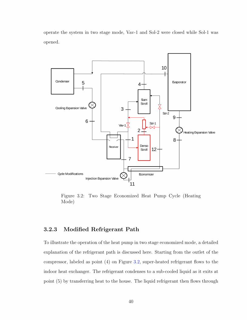
operate the system in two stage mode, Vav-1 and Sol-2 were closed while Sol-1 was

opened.

Siam Scroll

Denso Scroll

Receiver

EvaporatorCondenser

Cooling Expansion Valve

Injection Expansion Valve

Heating Expansion Valve

Vav-1 Sol-1

Sol-2

EconomizerCycle Modifications

1

45

6

7

8

9

10

11

12

3

2

Figure 3.2: Two Stage Economized Heat Pump Cycle (HeatingMode)

3.2.3 Modified Refrigerant Path

To illustrate the operation of the heat pump in two stage economized mode, a detailed

explanation of the refrigerant path is discussed here. Starting from the outlet of the

compressor, labeled as point (4) on Figure 3.2, super-heated refrigerant flows to the

indoor heat exchanger. The refrigerant condenses to a sub-cooled liquid as it exits at

point (5) by transferring heat to the house. The liquid refrigerant then flows through

40

the cooling expansion valve to the power receiver. The cooling expansion valve is

always fully opened when the system is operated in heating mode. The power receiver

serves two purposes in the cycle. First it ensures that a supply of liquid is available to

the expansion valves, and second, it provides additional super-heat to the suction gas

for compressor protection. From the receiver, the liquid refrigerant at point (7) is split

into two streams. The injection stream is expanded through the injection expansion

valve to point (11) where it is then evaporated to a high vapour mass fraction state

at point (12) which is injected between the two compressors through Sol-1. The main

stream at point (7) is further sub-cooled as it flows through the economizer to point

(8) where it is expanded to point (9) through the heating expansion valve. It then

travels through the outdoor heat exchanger where it is evaporated to a super-heated

vapour at point (10) by absorbing heat from the ambient air. The main stream then

flows through the power receiver to point (1), which increases the amount of super-

heat of the vapour, before it enters the suction port of the LP compressor. The

refrigerant exits the LP compressor at point (2) where it is mixed with the injection

stream from Sol-1, which reduces its temperature as it passes through point (3) before

it enters the HP compressor. A picture of the modified heat pump is shown in Figure

3.3.

3.3 Control

In order to have direct control of the operating conditions in the heat pump, a new

control system and auxiliary equipment were developed to replace the existing controls

which offered limited user inputs. Table 3.2 outlines the individual components that

were controlled.

41

Figure 3.3: Modified Heat Pump

3.3.1 System Controller

The controller used was a National Instruments (NI) Compact RIO (cRIO) 9074. The

NI cRIO-9074 is an embedded controller that runs the LabVIEW real-time operating

system. It includes a 400 MHz processor, 128 MB of ram, 512 MB of storage and

contains a Field Programmable Gate Array (FPGA). The operation of an FPGA is

outlined in Appendix B. This controller uses the NI C-series modules for inputs and

outputs which can be interchanged depending on the needs of the user. The modules

used for this work are outlined in Table 3.3.

3.3.2 LP Compressor

The LP compressor was operated using a Hitachi WJ-200-022LF variable frequency

drive (VFD). This VFD was chosen as it is designed to drive permanent magnet

motors. The compressor speed was controlled using a 0 - 10 Vdc signal from the NI

42

Table 3.2: Controlled Components

Component # to control Component Input

LP Compressor 1 Three Phase Power, Variable Fre-quency/Voltage/Amperage

HP Compressor 1 Three Phase Power, Variable Fre-quency/Voltage/Amperage

Expansion Valve 3 Four Phase Stepper Motor CoilSolenoid 2 120 Vac Power

4 Way Valve 1 240 Vac PowerOutdoor Fans 2 300 Vdc Power, 12 Vdc, and 0 - 6 Vdc

Speed Control

Table 3.3: NI cRIO-9074 Modules

Module # Type # of Channels Function

1 9217 4 100 Ω RTD2 9217 4 100 Ω RTD3 9217 4 100 Ω RTD4 9217 4 100 Ω RTD5 9219 4 Universal Analog Input6 9263 4 0 - 10 V Analog Output7 9401 8 High Speed Digital Input/Output8 9401 8 High Speed Digital Input/Output

cRIO-9074 controller. Table 3.4 contains the parameters that were used to program

the VFD.

3.3.3 HP Compressor

The HP compressor was operated using two different VFDs during the experiment.

Initially a Hitachi SJ700-075LFUF2 was used. However, once it was installed it be-

came apparent that the HP compressor was constructed using a permanent magnet

motor and the SJ700 (SJ) series of VFDs is not designed to control these types of

motors. Due to budgetary restrictions, initial testing was conducted using this VFD.

The compressor was able to be operated for a small speed range using the simple

43

Table 3.4: Denso Motor Parameters

Parameter Value

Motor Capacity 2.2 kWMotor Poles 6

Motor Voltage 208 VacMotor Amperage 8 Arms

Motor Speed 340 Hz

voltage/frequency mode of this drive. This mode operates the motor by controlling

the voltage applied to the windings for a given frequency based on table data that is

entered by the user. After a portion of the testing was completed, a more suitable Hi-

tachi WJ200-075LF (WJ) VFD became available and was installed. The performance

of the system with the new VFD was compared to the data collected with the old

VFD and the difference was found to be negligible. The only benefit was an increase

in the controllability of the compressor which was not exploited for this work.

Table 3.5 outlines the parameters that were used to program the WJ VFD. The

compressor speed was controlled using a 0 - 10 Vdc signal from the NI cRIO-9074

controller.

Table 3.5: Mitsubishi Motor Parameters

Parameter Value

Motor Capacity 7.4 kWMotor Poles 6

Motor Voltage 200 VacMotor Amperage 37 Arms

Motor Speed 360 Hz

44

3.3.4 Expansion Valves

The expansion valves were linear type valves which use a stepper motor to control

their position. They are constructed with four electrical coils that were energized

in a specific order to control the rotation. A FPGA code and an external current

amplification circuit were used to control these valves during testing. A detailed

explanation of the expansion valve control system can be found in Appendix C.

3.3.5 Solenoids and 4-Way Valve

The 4-way valve was used to switch the location of the evaporator and the condenser

within the cycle. This allowed the system to provide either heating or cooling de-

pending on the position of the valve. The solenoids were used to change the location

of the economized vapour injection. This allowed for the vapour to be injected either

at the original mid-compressor location, or at a new location between the LP and HP

compressors. The solenoids and 4-way valve were operated by energizing electrical

coils. A set of relays were used to control the solenoids and the 4-way valve from

within the control software.

3.3.6 Fans

The fans in the outdoor unit were capable of variable speed operation. They required

a 300 Vdc main power supply, a 15 Vdc power supply and a 0 - 6.5 Vdc signal to

operate. A 300 Vdc power supply was constructed that rectified a 208 Vac power

source. A two channel Sorensen bench top power supply was used to provide the 15

Vdc power supply and the 0 - 6.5 Vdc control signal. The fans were run at their

maximum speed during testing to simplify the control of the system. A detailed

explanation of the fan control circuits can be found in Appendix D.

45

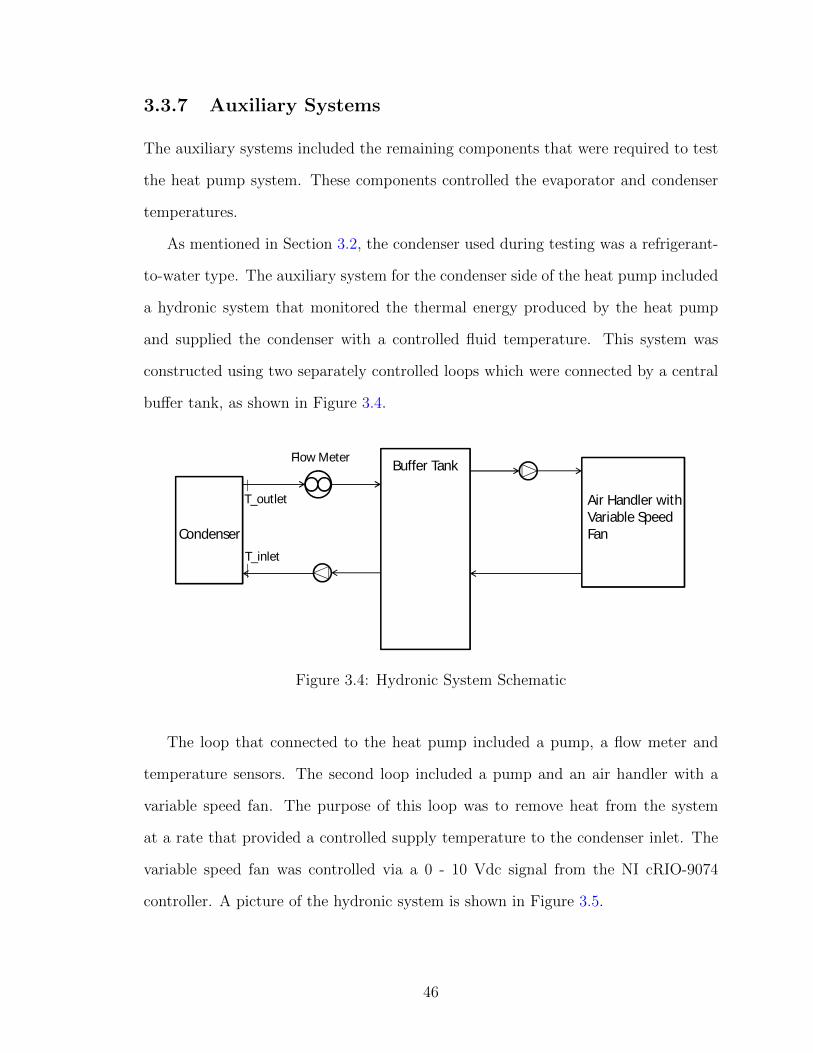
3.3.7 Auxiliary Systems

The auxiliary systems included the remaining components that were required to test

the heat pump system. These components controlled the evaporator and condenser

temperatures.

As mentioned in Section 3.2, the condenser used during testing was a refrigerant-

to-water type. The auxiliary system for the condenser side of the heat pump included

a hydronic system that monitored the thermal energy produced by the heat pump

and supplied the condenser with a controlled fluid temperature. This system was

constructed using two separately controlled loops which were connected by a central

buffer tank, as shown in Figure 3.4.

Air Handler withVariable SpeedFan

Buffer Tank

CondenserT_inlet

T_outlet

Flow Meter

Figure 3.4: Hydronic System Schematic

The loop that connected to the heat pump included a pump, a flow meter and

temperature sensors. The second loop included a pump and an air handler with a

variable speed fan. The purpose of this loop was to remove heat from the system

at a rate that provided a controlled supply temperature to the condenser inlet. The

variable speed fan was controlled via a 0 - 10 Vdc signal from the NI cRIO-9074

controller. A picture of the hydronic system is shown in Figure 3.5.

46

Figure 3.5: Hydronic System

The evaporator temperature was controlled by placing the outdoor unit inside a

refrigerated container. The original intent was to test the system at outdoor temper-

atures of -40C and also have control over the ambient conditions. However, during

commissioning it was discovered that the lower limit of the container’s refrigeration

cycle was -30C and that only slightly colder temperatures could be achieved when

the heat pump was operating. A picture of the refrigerated container is shown in

Figure 3.6.

3.3.8 Programming

The programming was conducted using NI LabVIEW and it was implemented through

four separate applications that were distributed across three pieces of hardware.

The NI cRIO-9074, outlined in Section 3.3.1, was used to control everything within

the heat pump and also acted as the main data logger for the system.

47

Figure 3.6: Refrigerated Container

A second NI cRIO-9074 was used to run the hydronics lab. This controller was

programmed to maintain the liquid supply temperature to the heat pump during

testing.

Lastly, a desktop PC was used to control and provide feedback for the system via

a user interface. A detailed explanation of the software can be found in Appendix E.

3.3.9 Instrumentation

The system instrumentation was split into two categories: critical and support. The

instrumentation used to measure the performance of the system was considered crit-

ical and all efforts were made to minimize the inherent errors associated with their

measurements. The additional instrumentation used for control and system operation

was considered as support.

48

3.3.9.1 Critical Measurements

Critical measurements included all parameters that were required to determine the

heating capacity (QH) and coefficient of performance (COP) of the heat pump. The

heating capacity was calculated using Equation 3.1.

QH = V– ρCp∆T (3.1)

where V– is the volumetric flow rate of the fluid, ρ is the density of the fluid, Cp is the

heat capacity of the fluid, and ∆T is the temperature differential of the fluid across

the condenser.

The COP was calculated using Equation 3.2.

COP =QH

Pelec(3.2)

where QH is the heating capacity as defined in Equation 3.1 and Pelec is the electrical

power required to operate the system.

The volumetric flow rate was measured using a Sparling Economag FM-618-0D1-

000-01 flow meter. This meter operates using Faraday’s Law of Magnetic Induction

which is defined in Equation 3.3.

EV = BLV (3.3)

where E is the induced voltage, B is the flux density of the magnetic field, L is the

distance between the electrodes, and V is the bulk flow velocity of the liquid. The

meter imposes a magnetic field across the pipe and uses electrodes to measure the

induced voltage which is then converted to a volumetric flow rate inside the meter

based on the cross sectional area of the pipe.

49

The temperature differential was measured using two Omega P-M-1/10-1/8-6-0-

T-3 platinum resistance temperature detectors (RTD). RTDs operate based on the

principle that the resistance of a conductor is a function of its temperature. The

sensors selected were 100 Ω, 1/10 DIN accuracy 4 wire probes that were placed in

thermowells located as close to the condenser as was possible. The thermowells were

filled with a thermally conductive grease, and the piping and wiring were insulated

as much as possible.

The fluid properties were assumed to be constant throughout testing and the

values used in calculations were based on an operating temperature of 45C. A detailed

study of the implications of this assumption are included in Section 4.4.

The electrical power, Pelec, included the power required to drive both compres-

sors, the outdoor unit fans, the indoor unit fans, and the internal electronics. Due

to the nature of the experiment, the indoor unit fan power could not be included

because this unit is internal to the hydronic system. The internal electronics were

also replaced with NI equipment which was not representative of what would be used

to operate a system like this in real-world applications. For these reasons, only the

outdoor unit fan power and the power supplied to the compressors were included in

the COP measurement. This may have caused the COP to show the system as over

performing. However, modern air handlers with electronically commutated motors

typically have very low power consumption compared to the total consumption of

the heating system. Also, the consumption of the electronic controller was assumed

to be negligible, as they typically consume less than 20 W. Lastly, the outdoor fan

unit was determined to have a variable consumption of between 50 W to 300 W and

during testing the fan was operated at full speed. In a market ready system, the fan

speed would be reduced to match the capacity of the system to save power. Together,

these factors resulted in more power consumption than was necessary, and any over

statement of the COP was considered to be minimal.

50

All electrical measurements were made using two Tektronix PA-4000 power an-

alyzers. These power analyzers are extremely flexible and are necessary to measure

the advanced waveforms that are present in VFD systems. Each power analyzer in-

cludes four independent channels for the measurement of voltage and current. Both

of the compressors were three phase machines and required three channels each. Each

PA-4000 was programmed to measure three phase power and was set to pulse width

modulation (PWM) mode. This mode allows for the high order harmonics, which are

present when using VFDs, to be included in the measurement which was necessary to

accurately measure the compressor power consumption. To ensure safe connections

could be made during the measurements, electrical patch boxes, shown in Figure 3.7,

were constructed to allow for the connection of insulated banana connectors between

the power circuit and the PA-4000 analyzer. Five patch boxes were constructed and

installed before and after each VFD and also at the fan circuit.

Figure 3.7: Power Measurement Patch Box

51

All of the measurements performed by the power analyzers were recorded on the

desktop computer via a connection across the local network using LabVIEW and

the standard commands for programmable instruments (SCPI) protocol. SCPI is a

standardized text-based communication syntax which is widely used by laboratory

instruments and makes these connections trivial.

3.3.9.2 Support Instrumentation

The support instrumentation provided the measurements that were used to control

and monitor the refrigeration cycle. Pressure measurements were taken for the con-

denser, the evaporator and the intermediate pressures. These measurements were

used to calculate the saturation temperatures of the refrigerant for control purposes.

The evaporator and intermediate pressures were measured using Omega PX-303-

300A5V pressure transducers and the condenser pressure was measured using an

Omega PX409-500AI transducer. Theses sensors operate by measuring the strain

present in a stainless steel diaphragm. The measured fluid is in contact with one side

of the diaphragm while the other side is exposed to either ambient air or a vacuum

depending on whether the sensor measures gauge or absolute pressure. The PX-303

transducers measured gauge pressure while the PX409 transducer measured absolute

pressure.

Twelve temperatures were measured at locations throughout the refrigerant cycle

using platinum RTDs. For these temperature measurements Omega PR-20-2-100-

1/8-2-E-T sensors were used. These are class A RTDs which are less expensive than

the 1/10 DIN RTDs used for the critical measurements. The sensors were installed

by surface mounting the probes on the copper pipes and insulating them as much as

possible. Figure 3.8 illustrates the installation of these probes.

52

Thermal Paste

Insulation

RTD

Electrical Tape

Copper Pipe

Figure 3.8: Surface Mounted RTD Section View

Figure 3.9 shows the location of the pressure sensors and the eleven temperature

sensors that were installed on the heat pump. The remaining temperature sensor was

used to measure the temperature of the air that was supplied to the evaporator.

3.4 Closing Remarks

An experimental apparatus was constructed and instrumented to allow the perfor-

mance of a two stage economized heap pump to be characterized during cold weather

operation. The following chapter outlines the work that was done to determine the

uncertainty associated with the instrumentation.

53

Siam Scroll

Denso Scroll

Receiver

Outdoor HX

Condenser

Cooling Expansion Valve

Injection Expansion Valve

Heating Expansion Valve

Vav-1Sol-1

Sol-2

Economizer

P,T

T

T

P,T

P,T

T

T

T

T

TT

Evaporator

Figure 3.9: Installation Location of Support Instrumentation

54

Chapter 4

Uncertainty

To ensure the accuracy of the critical measurements outlined in Section 3.3.9.1, an

uncertainty analysis was conducted using the procedure outlined by Moffat [19]. For

each measured parameter, the associated error can be quantified by its precision

error and its bias error. The precision error is used to describe the random error that

occurs during an experiment while the bias error is used to describe the repeatable

error margin for a single measured value.

4.1 Bias Error

Each measured value has multiple sources of bias associated with it that correspond

to the individual components which make up the measurement system. These vary

depending on the type of measurement being performed. The bias for the measured

quantity can be determined by combining the bias associated with each component

in the measurement system using Equation 4.1.

Bj =√B2i (4.1)

where Bi is the bias for a given component in the measurement system and Bj the

bias for the quantity produced by the measurement system.

The total bias error for a derived quantity can be computed by combining the indi-

vidual bias error associated with each contributing measured value with a sensitivity

factor, θj, using Equation 4.2.

55

BT =

√∑j

(θjBj)2 (4.2)

where BT is the total bias error for the derived quantity, and θj is the sensitivity

coefficient as described my Moffat [19], such that:

For: r = f(P1, P2, ...Pi)

where the derived quantity, r, is a function of the measured quantities, Pi. The

sensitivity coefficient is defined using Equation 4.3.

θj =∂r

∂Pj(4.3)

4.2 Precision Error

The precision error for the average derived quantities, S, can be calculated using

the standard deviation, S, and the number of instantaneous derived measurement

quantities, N , recorded over the sampling period, as shown in Equation 4.4.

S =S√N

(4.4)

4.3 Overall Uncertainty

The overall uncertainty margin, U , for the average derived quantity can be determined

by combining the total bias error and the precision error weighted by a student T

statistic, ts, as shown in Equation 4.5.

U =√B2T + tsS (4.5)

56

where the student T statistic is chosen based on the number of samples and the

desired confidence interval. For the testing conducted, the average derived values

were based on a sample size of 300. When the number of samples is greater than

120, the standard deviation is considered to be an accurate representation of the

population. Therefore, the student T statistic was replaced with a value of 2 to give

a confidence interval of 95.4%.

4.4 Heating Capacity Uncertainty

The uncertainty of the heating capacity measurement was calculated using the ap-

proach outlined above. A sample calculation has been included in this section for

clarity. The heating capacity was calculated using Equation 3.1. The example given

here corresponds to a flow rate of 0.35 L/s and a temperature differential of 2.5C

with a mean fluid temperature of 45C which is representative of what was observed

during testing.

The volumetric flow rate was measured using the Sparling flow meter as outlined

in Section 3.3.9. The meter was scaled to a maximum flow of 30.28 L/min and

outputted a 4 - 20 mA signal that is linearly proportional to the flow rate. The signal

was measured using a NI-9219 universal 24 bit input module that was configured to

measure 0 - 25 mA. The software calculated the flow rate using Equation 4.6 which

converts the mA signal from the meter to a flow rate in L/s.

V– = (A− 0.004) ∗ 31.545 (4.6)

where V– is the volumetric flow rate of the fluid and A is the measured signal in

amps. Table 4.1 shows the rated component level accuracies and the corresponding

bias error associated with the flow rate measurement.

57

Table 4.1: Heating Capacity Component Bias Errors for ExampleCase

Sparling Meter Rating [Flow = 0.35 L/s]Rated bias 0.75 % Rate

Sparling Meter Bi ComponentsBSparling ± 0.00263 L/s

NI 9219 Rating[Signal = 0.0151 A]Gain Error ± 0.1 % ReadingOffset Error ± 30 ppm Range

NI 9219 Bi ComponentsBNIGain

± 3.5x10-4 L/sBNIOffset

± 2.37x10-5 L/s

Volumetric Flow Rate Bias ErrorBj ± 2.65x10-3 L/s

The heat transfer fluid used was Diversitech ProTek-PLUS which is a 95% pure

propylene glycol fluid with corrosion inhibitors making up the balance. The fluid

was diluted during commissioning and the mixture was determined by measuring

the fluid’s refractive index using an ATAGO PAL-RI meter. Diversitech does not

publish the heat capacity of its fluids so the refractive index was used to look up the

corresponding values in the Dow document, A Guide to Glycols [20] which contains

information about aqueous solutions of propylene glycol and is available on their

website.

As testing was conducted with the heat transfer fluid operating in the temperature

range of 40C to 50C, the values for both the density and the heat capacity were taken

at 45C, and these values were assumed constant throughout testing. To account for

the variation in the fluid properties caused by changes in fluid temperature, the bias

of the fluid properties were based on the variation of the fluid properties across the

temperature range of 40C to 50C. These fluid properties and their associated bias

errors are shown in Table 4.2.

58

Table 4.2: Heat Transfer Fluid Properties and Associated Bias Er-rors for Example Case

Aqueous Propylene Glycol SolutionRefractive Index [n] 1.3604Glycol % by Volume 23.4Glycol % by Weight 24

Densityρ45C 1.007 kg/LBρ ± 0.003 kg/L

Heat CapacityCp45C 4.0386 kJ/kg CBCp ± 0.00586 kJ/kg C

The temperature difference was measured using two platinum RTDs that were

connect via four wire circuits to a NI 9217 24 bit RTD input module. The resistance

was measured and converted to temperature in software using a calibrated polynomial

fit whose associated bias error was orders of magnitude smaller than the other relevant

sources of error and was therefore neglected. Information regarding the polynomial

fitting is outlined in Section 4.6.1. Table 4.3 outlines the sources of error that were

considered for the temperature measurement.

Table 4.3: Temperature Differential Bias Error

1/10 DIN Platinum RTDBRTD ± 0.08C

NI 9217 RTD ModuleBdaq ± 0.15C

Temperature Bias ErrorBTemperature ± 0.17C

Differential BiasB∆T ± 0.24C

The total bias error for the derived quantity QH was calculated using Equation

4.2. The sensitivity factors, total bias errors, and contributing bias terms are shown

59

Table 4.4: Heating Capacity Sensitivity Factors and Total Bias Error

Heating Capacity Sensitivity Factors for Example CaseFactor Equation Example Value

θ ˙V– = ∂Q

∂˙V–

θ ˙V– = ρCp∆T 10.167 kJm3

θρ = ∂Q∂ρ

θρ = V– Cp∆T 3.534 kJ∗m3

kg∗s

θCp = ∂Q∂Cp

θCp = V– ρ∆T 0.881 kg∗Cs

θ∆T = ∂Q∂∆T

θ∆T = V– ρCp 1.423 kJs∗C

Contribution to Derived Quantity Bias Error for Example CaseTerm Total Bias Error [kW]θ ˙V– B ˙V– 0.027

θρBρ 0.011θCpBCp 0.005θ∆TB∆T 0.341

Heating Capacity Total Bias Error [BT ]BQ ± 0.343 kW

in Table 4.4. As expected, the bias errors associated with the temperature difference

are the dominating contributers to the total bias error of the derived heating capacity.

The precision error was combined with the total bias error using Equations 4.4

and 4.5. For this example, the standard deviation used was based on typical values

observed during testing. Table 4.5 shows the relevant parameters used to calculated

the total uncertainty of the measured heating capacity of the system.

Table 4.5: Heating Capacity Total Uncertainty for Example Case

Precision Error Calculation [2 Standard Deviations]Parameter Definition Example ValueS Standard Deviation of Average Derived Quantity 0.015N Number of Samples Measured 300S 8.66x10-4

Heating Capacity Total Uncertainty [U ]U ± 0.346 kW

60

For this example, the thermal output was 3.56 kW which represents an error of

9.7% for the derived quantity.

4.5 COP Uncertainty

The same process was used to calculate the uncertainty of the COP measurement.

The example used in Section 4.4 will be reused in this section, assuming an input

work of 1.5 kW.

The COP was calculated using Equation 3.2. The power was measured using

the PA-4000 power analyzer which measured three phase voltage and current and

calculated the power internally. According to the manual, the power measurement

accuracy of the analyzer is defined using Equation 4.7.

Pacc = (VrmsaccArmsPF )

±(ArmsaccVrmsPF )

±(VrmsArms(cos θ − cos(θ ± (V h1pherr ± Ah1pherr)))

(4.7)

where Vrms is the measured root mean square (RMS) Voltage, Arms is the measured

RMS Amperage, PF is the measured power factor, θ is the measured phase angle,

Vrmsacc is the accuracy of the voltage reading, Armsacc is the accuracy of the amperage

measurement, V h1pherr is the accuracy of the phase of the first voltage harmonic, and

Ah1pherr is the accuracy of the phase of the first amperage harmonic.

Each of the accuracy terms listed have different values that depend on the voltage,

current and frequency ranges the power analyzer was configured for during measure-

ment. As this calculation is quite complex and lengthy, the details of this process

are not included in this thesis. However, the parameters listed in Equation 4.7 that

61

were used during the uncertainty analysis are included in Appendix F, along with the

calculated bias errors associated with the power measurements.

The largest bias error for the three phase power measurement that was calculated

during testing was 0.0043 kW. This value is used for the following example.

The bias errors that were calculated are shown in Table 4.6 along with the sensi-

tivity factors and the total bias error for the COP measurement.

Table 4.6: COP Bias Error Calculation for Example Case

Bias ComponentsBQ ± 0.343 kW

Belec ± 0.0043 kW

Sensitivity FactorsFactor Equation Example Value

θPelecθPelec

= ∂COP∂Pelec

= − QP 2elec

1.582 1kW

θQ θQ = ∂COP∂Q

= 1Pelec

0.667 1kW

COP Total Bias ErrorBCOP ± 0.229

The standard deviation for this example was taken as a typical value observed

during testing where S was in the range of 0.015. Table 4.7 shows the precision error

and the total uncertainty calculation for the COP.

Table 4.7: COP Precision Error and Total Uncertainty for ExampleCase

Precision ErrorS 0.015N 300S ± 8.66x10-4

Total UncertaintyU ± 0.233

For this example, the COP was 2.37 and the corresponding error would be 9.8%.

62

4.6 Calibration and Uncertainty Reduction

As the dominant source of uncertainty in the derived quantities is associated with

the temperature differential measurement, additional effort was made to improve the

bias associated with these measurements.

The procedure used here is based on the steps outlined in Sections 4.1, 4.2, and

4.3 with an alternate approach used to quantify the bias error associated with the

temperature measurements. The first approach assumed that the bias errors in the

system were independent from one another and took the worst case approach when

combining them, where each bias increases the total bias of the measurement system.

This approach can be said to be valid for interchangeability. This means the calculated

uncertainty is valid for any physical hardware that shares the same rated bias and is

combined in the same configuration.

The modification used here considers the measurement system as a whole, and

results in the direct measurement of the total bias error for the derived quantity

BTemperature. It is based on two assumptions. First, the rated bias of a component

includes a level of quality control during manufacturing and an individual component

could have a bias that is lower than its rating. Second, it is conceivable that when

real devices are combined to create a measurement system, some of the bias errors

may combine to reduce the total bias of the measured quantity.

Using these assumptions, this procedure presents a systematic approach to quan-

tifying and monitoring the bias of a measurement system using a calibrated reference

system. It requires the use of additional specialized equipment and it is not valid for

interchangeability. This means the bias is specific to the hardware as it is installed,

and any changes made to the components or system would require the procedure to

be repeated. The procedure is split into three steps: calibration, quantification and

verification which are described in the following sections.

63

4.6.1 Calibration

The calibration procedure requires the use of a calibrated reference thermometer

and an environment that is stable enough to allow comparison between the reference

thermometer and the temperature measurement system. A Fluke 5616-12 Secondary

Platinum Resistance Thermometer (SPRT) and a Fluke 1502A SPRT digital readout

were used as the calibrated reference thermometer. A calibrated Fluke 7340 liquid

bath that was filled with Dow Corning silicone oil 200.10 was used as the stable

environment.

As the calibration was conducted by considering the measurement system as

whole, the procedure was conducted after the RTDs were installed in the experi-

mental apparatus and connected to the data acquisition system (DAQ). The cabling

allowed the RTDs to be placed in the bath without requiring any electrical discon-

nections and the resistance readings were recorded by the DAQ. The SPRT was also

placed into the bath and the readout was recorded via a serial connection with a desk-

top computer. Both data sources were recorded at ten second intervals. The bath

was programmed to span the temperature range of 40C to 61C in 3C steps where

it would hold the temperature at each step for 20 minutes once the bath reached

stability. The dataset was reduced by averaging the last 5 minutes of data for each

temperature point.

Lastly, the resistance measurements of the RTDs were regressed to the tempera-

ture measurements of the SPRT using a second order polynomial. The polynomials

were added to the DAQ software to allow for direct temperature readings with units

of degrees Celsius. This step produced a calibrated temperature measurement system

for each RTD channel that was used for the remainder of the procedure. This step

was also conducted for the support RTDs with the bath spanning the range of -30C

to 110C in 10C increments.

64

4.6.2 Bias Quantification

The approach used to quantify the bias of the calibrated temperature measurement

system was based on a statistical analysis of the calculated error between the cali-

brated temperature measurements and the measurements of the SPRT. This required

a dataset that captured the long term drift and instabilities that were present in the

system. As the amount of data required to accomplish this was unknown, an assump-

tion was made based on the nature of the measurement, and the verification stage

was used to confirm an appropriate sample was acquired.

The bath was set to 50C and data were collected for multiple days. Ideally,

this procedure would have been repeated for a variety of temperatures spanning the

operating range of the system, but due to time restrictions, only one temperature was

used for the quantification stage.

Figure 4.1 plots the raw temperature readings directly against the readings from

the SPRT. It shows a normal distribution in the measured error relative to the SPRT.

The error for each sample was calculated using Equation 4.8

εT = TCalibrated − TReference (4.8)

where εT is the measured error associated with a sample in the data.

Figure 4.2 plots the time series of the calculated error in the readings from the

RTDs relative to the SPRT. It shows that each channel contains some noise, as well as

a diurnal fluctuation, with Twaterout fluctuating greater and in opposition to Twaterin.

The difference in rising edge to trailing edge slope in the Twaterout measurement is

thought to be caused by the morning sun warming a portion of the measurement

system. However, it is not the intention of this thesis to determine the cause of the

errors, but simply to quantify them.

65

50.200

50.205

50.210

50.215

50.220

50.225

50.230

50.235

50.240

50.245

50.250

50.200 50.205 50.210 50.215 50.220 50.225 50.230 50.235 50.240 50.245 50.250

Calib

rate

d RT

D

SPRT

Calibrated RTD Compared to SPRT

T_water_in T_water_out Linear

Figure 4.1: Measured Temperature vs. SPRT Reading

Figures 4.1 and 4.2 each give a representation of how well the calibrated temper-

ature measurements agree with that of the reference SPRT. If this comparison was

continued during the experimental work, then the calculated bias of the data would

be an exact measurement of the bias of the temperature system with respect to the

SPRT. Unfortunately this is not realistic, as the sensors cannot be in the bath during

experimentation. Therefore, this measured approach was used to estimate the bias

in the temperature measurement system.

The bias errors associated with the temperature measurements were calculated by

combining the absolute value of the mean of the errors with three standard deviations

using Equation 4.9.

BTemperatureMeasurement = |XεT |+ 3 ∗ SεT (4.9)

66

-0.025

-0.02

-0.015

-0.01

-0.005

0

0.005

0.01

0.015

0.02

0.025

0 5000 10000 15000 20000 25000

Tem

pera

ture

Err

or (T

_RTD

-T_

SPRT

) [C]

Data Point (x10s)

Measured Error of RTDs Relative to SPRT Reading at 50 C

T_water_in-SPRT T_water_out-SPRT

Figure 4.2: Time Series of Long Term Temperature Difference Data

where XεT and SεT are the mean and standard deviation of the errors respectively. The

calculated bias for TWaterOut was used for both the inlet and outlet water temperature

measurements in order to slightly overestimate the bias of the temperature differential

and to add additional confidence to the data that were collected. Since the SPRT

and readout were used as the reference for comparison and they each contain bias

error terms, their bias errors were combined with the calculated bias of the data using

Equation 4.1. The bias errors for the temperature measurements and the calculated

temperature differential that resulted from this approach are shown in Table 4.8.

This approach shows a significant improvement over the bias error that was cal-

culated in Table 4.3. If the example from Sections 4.4 and 4.5 is repeated using the

measured bias error, the uncertainty of the measured heating capacity is reduced

from ± 0.346 kW to ± 0.072 kW and the error is reduced from 9.7% to 2%. The

uncertainty and error of the COP measurement is improved by similar amounts.

67

Table 4.8: Measured Temperature Differential Bias Error [B∆T ]

Measured Error Absolute MeanXεTWaterIn

0.0020C

XεTWaterOut0.0004C

Measured Error Standard DeviationσTWaterIn

0.0023CσTWaterOut

0.0067CCalculated Bias Relative to SPRTBTWaterIn

0.0088CBTWaterOut

0.021CSPRT Bias Error

BSPRT ± 0.011CBReadout ± 0.009C

Combined Bias ErrorBTemperatureMeasurement ± 0.0254CB∆T ± 0.036C

4.6.3 Verification

The verification step is intended to show that the measured bias error is repeatable

and give confidence that the original dataset was large enough to accurately quantify

the bias error.

Verification is the process of occasionally checking the calibrated temperature

measurement system against the reference system. This is done by comparing the

measured relative bias between the measured temperatures and the reference probe

with the relative bias that was calculated in Section 4.6.2. The frequency of veri-

fication should be representative of the criticality of the measurements in order to

give confidence in the measurement accuracy. For the experimental work presented

here, verification was done once testing was completed. The original calibration and

quantification procedures were conducted on September 25 and 26, 2014 respectively

and the verification was conducted on February 2, 2015. This was considered to be

reasonable as it would have captured any long term drift in the electronics that occur

due to either time or seasonal changes in temperature and humidity.

68

During verification, the temperature probes were returned to the temperature bath

with the SPRT, and data were collected at 30C and 50C with each temperature

checked twice to increase the sample size of the data. Data were recorded for five

minutes at each temperature at a rate of one sample per second. This produced four

sets of data consisting of 300 samples for each of the temperature channels, as shown

in Figures 4.3 and 4.4.

30.150

30.160

30.170

30.180

30.190

30.200

30.210

30.220

30.230

30.240

30.250

30.150 30.160 30.170 30.180 30.190 30.200 30.210 30.220 30.230 30.240 30.250

Calib

rate

d RT

D

SPRT

Post Testing Sensor Verification (30 C)

T_water_in T_water_outlet Linear

Figure 4.3: Verification Data 30C

The measured bias error was calculated for each dataset using the method outlined

in Section 4.6.2. The results shown in Table 4.9 verify the quality of the data that

were used during quantification. The highest relative bias error calculated during

verification was 0.022C which is 0.001C greater than the relative bias that was

calculated in Section 4.6.2. This increase indicates a negligible difference between

the calculated uncertainties of the results, therefore, the procedure outlined here was

considered to be a valid method of reducing the uncertainty of the measurement

system.

69

50.150

50.160

50.170

50.180

50.190

50.200

50.210

50.220

50.230

50.240

50.250

50.150 50.160 50.170 50.180 50.190 50.200 50.210 50.220 50.230 50.240 50.250

Calib

rate

d RT

D

SPRT

Post Testing Sensor Verification (50 C)

T_water_in T_water_outlet Linear

Figure 4.4: Verification Data 50C

Table 4.9: Measured Temperature Bias Error During Verification

TWaterInlet TWaterOutlet

TBath |XεT | σεT BTRelative|XεT | σεT BTRelative

30C 0.012C 0.003C 0.019C 0.002C 0.002C 0.010C50C 0.014C 0.002C 0.020C 0.010C 0.002C 0.017C50C 0.014C 0.003C 0.022C 0.012C 0.002C 0.019C30C 0.010C 0.002C 0.015C 0.004C 0.002C 0.010C

70

Chapter 5

Test Plan and System Operation

The experimental work was intended to quantify the steady state performance of

the system when operated at ambient temperatures that are present in Canadian

climates. Table 5.1 outlines the test matrix that was used during the planning stages

of the experiment.

Table 5.1: Test Matrix 50C Supply Temperature

Ambient Temperature [C]System Mode 0C -10C -20C -30C -40CSingle StageSingle Stage EconomizedTwo Stage Economized

During commissioning, it was discovered that the lowest temperature achievable

in the cold chamber was -31C. Also, the HP compressor outlet temperature was

above the rated maximum when the supply temperature was 50C. The test plan was

modified by removing the -40C test point and lowering the supply temperature to

40C to reflect these limitations. During single stage and single stage economized

operation, the HP compressor outlet temperature continued to be above the rated

maximum when the ambient temperature was below -23C. The test plan was further

modified to avoid single stage operation below this temperature. Table 5.2 shows the

modified version of the test matrix that was used during testing.

The system operating modes are defined as follows:

71

Table 5.2: Modified Test Matrix 40C Supply Temperature

Ambient Temperature [C]System Mode 0C -10C -20C -30CSingle Stage NASingle Stage Economized NATwo Stage Economized

• Single Stage - The original cycle configuration without economized vapour in-

jection.

• Single Stage Economized - The original cycle configuration with economized

vapour injection.

• Two Stage Economized - The modified cycle with interstage economized vapour

injection.

The cycle schematics for each of these operating modes are shown in Figure 5.1.

For all of these configurations, the HP compressor was initially operated at a fixed

speed of 90 Hz. This speed resulted in stable operation of the motor when the SJ

series VFD was used. Also, this speed kept the mass flow rates of each stage within a

range that would allow for operation in the two stage economized configuration. The

HP compressor was able to operate at much higher speeds; however, doing so would

increase the mass flow in the system beyond the operating range of the smaller LP

compressor. To investigate the effect the HP compressor speed had on the operating

performance, the tests were repeated with the HP compressor operating at 80 Hz

once the WJ series VFD was installed.

5.1 System Operation

The strategy used to test the system was developed during commissioning and allowed

for good stability with minimal downtime between test points.

72

Siam Scroll

Receiver

EvaporatorCondenser

Cooling Expansion Valve

Heating Expansion Valve

Economizer

(a) Single Stage

Siam Scroll

Receiver

Condenser

Cooling Expansion Valve

Injection Expansion Valve

Heating Expansion Valve

Economizer

Evaporator

(b) Single Stage Economized

Siam Scroll

Receiver

Condenser

Cooling Expansion Valve

Injection Expansion Valve

Heating Expansion Valve

Economizer

Denso Scroll

Evaporator

(c) Two Stage Economized

Siam Scroll

Denso Scroll

Receiver

Outdoor HX

Condenser

Vav-1Sol-1

Sol-2

Economizer

1

2

3

11

4

10

9

8

67

5

Evaporator

(d) Cycle State Points

Figure 5.1: System Operating Schematics

5.1.1 System Preheating

Each day the hydronic system, shown in Figure 3.4, needed to be preheated to the

testing temperature of 40C. As this system was recently commissioned, the only

source of fluid heating was the heat pump itself. Preheating was achieved by operating

the heat pump in single stage mode with the cold chamber set to 0C. This allowed

the buffer tank and hydronic system to be preheated within two hours. Once the

system was preheated, the heat pump was shut down and configured for the cycle to

be tested.

73

5.1.2 Startup Procedure

The heat pump was started each day using manual controls. The required support

equipment was powered and software was used to confirm communication with all

devices. The expansion valves were calibrated and manually set to either their fully-

opened or fully-closed position. Since the system was operating in heating mode, the

cooling expansion valve was opened and the heating and injection valves were fully

closed.

The pumps and fans were enabled, and the compressors were brought to their

minimum speeds. To avoid a slug of liquid entering the compressor at startup, the

heating expansion valve remained closed so the compressor suction would decrease the

mass of refrigerant that had accumulated in the evaporator during system shutdown.

Once the liquid was removed, the suction pressure would drop and the automatic

super-heat control algorithm was enabled to control the heating expansion valve.

5.1.2.1 Super-heat Control Algorithm

The super-heat control algorithm was used to control the amount of super-heat that

was present at the evaporator outlet. The saturation temperature of the evaporator

was determined by measuring its pressure, as outlined in Section 3.3.9.2, and looking

up the corresponding saturation properties in a table which was embedded in software.

The desired super-heat was calculated using Equation 5.1.

Tsuper−heat = Tevapoutlet − Tevapsaturation (5.1)

where, Tsuper−heat is the amount of super-heat that is present in the refrigerant at the

outlet of the evaporator, Tevapoutlet is the refrigerant temperature at state point 9, as

shown in Figure 5.1d, and Tevapsaturation is the refrigerant saturation temperature that

corresponds to the evaporator pressure.

74

During testing the super-heat was controlled at 8C using a Proportional-Integral-

Derivative (PID) feedback algorithm that was programmed into the main controller.

The algorithm functioned by reducing the error between the set point of 8C and the

super-heat calculated with Equation 5.1 by controlling the position of the heating

expansion valve. The details of the super-heat control algorithm are included in

Appendix G.

5.1.3 Economized Operation

During single stage economized operation, the injection expansion valve was opened

in small increments and the system was monitored to determine if further adjustments

were needed. In this mode of operation, there was no way to determine the amount of

refrigerant mass that was being injected into the compressor. Also, since the system

was not operated using the Mitsubishi controller, there was no way to confirm what a

normal injection rate was. For these reasons, the single stage economized tests were

reduced to a single ambient temperature in an attempt to reduce possible damage to

the compressor.

When operated in two stage economized mode, the injection was used to control

the amount of super-heat at the inlet of the HP compressor.

5.1.4 Intermediate Pressure

During the modelling study, the intermediate pressure was fixed by setting the satura-

tion temperature of the intermediate states directly. The ideal intermediate pressure

was then determined through trial and error. In the real two stage system, the in-

termediate pressure could not be controlled directly. However, it could be controlled

indirectly by varying the speed of the LP or HP compressor relative to the other.

This was illustrated with a study in EES which considered the effect that changing

the LP compressor speed had on an isentropic two stage compression process.

75

Figure 5.2 shows the two stage compression system that was considered for this

study.

1

2

3

Figure 5.2: Two Stage Compression Process

The compression process was assumed to be supporting a heat pump whose evap-

orator and condenser saturation temperatures were -20C and 40C respectively. The

HP compressor’s volumetric displacement was set to 33 cm3/rev and its rotational

speed was fixed at 1800 rpm. The LP compressor’s volumetric displacement was set

to 18 cm3/rev and its rotational speed was increased from 1000 rpm to 6400 rpm in

200 rpm increments. These volumetric displacements and speeds are representative

of the equipment that was used during testing. The resulting intermediate pressures

were plotted against the LP compressor speed, shown in Figure 5.3.

This shows that there is an almost linear relation between the LP compressor speed

and the intermediate pressure for a given HP compressor speed. This result, combined

with the effect that intermediate pressure has on COP, as outlined in Section 2.7.1,

indicates that there is an ideal LP compressor speed that will produce the maximum

COP for the system at each ambient temperature.

76

0

200

400

600

800

1,000

1,200

1,400

1,600

0 1,000 2,000 3,000 4,000 5,000 6,000 7,000

Inte

rmed

iate

Pre

ssur

e [k

Pa]

LP Speed (rpm)

Intermediate Pressure vs. LP compressor Speed(-20°C Evaporator, 40°C Condenser)

Figure 5.3: Intermediate Pressure vs. LP Compressor Speed

5.1.5 LP Compressor

The LP compressor speed was varied at each operating point to locate the ideal

intermediate pressure and to characterize its effect on the system performance.

5.1.6 Steady State Operation

Once the system was operating using the super-heat control algorithm, it was allowed

to run until the HP compressor discharge temperature, measured at state point 4 on

Figure 5.1d, stabilized. This parameter was the slowest to stabilize in the system and

for deviations of 5C to 10C, no measurable change in performance was observed.

For these reasons, the HP discharge temperature was used as an indicator of system

stability and the system was considered to be operating at steady state when the

deviation in this parameter was less than 1C/min. Once stabilized, the system was

operated for a minimum of twenty minutes. The final five minutes of data collected

were used to create a data point for analysis.

77

After data for a test point were collected, the temperature of the cold chamber

was reduced to the next test point and the system was allowed to stabilize again.

This approach proved to have the shortest wait time between system stability when

compared to changing the system configuration while keeping the cold chamber at a

constant temperature.

5.1.7 Defrost Cycle

During commissioning of the heat pump, the evaporator required defrosting only

once. This was accomplished by operating the heat pump in single stage mode with

the reversing valve in the cooling position. The evaporator fans were shut off and the

system was run until the evaporator was visibly free of frost. Defrost is a challenging

problem for heat pump manufactures as it requires additional energy that is not

used to provide heating within the home. This reduces the long term performance

of a heat pump and requires an intelligent strategy to ensure minimal energy is used

during the defrost cycle. As testing here was limited to characterizing the steady state

performance of the heat pump, the impact of the defrost cycle was not considered.

During testing, no frost accumulation was observed on the evaporator.

5.2 Closing Remarks

A series of experiments were conducted for the operating conditions that are outlined

in Table 5.2. The following chapter will discuss the results of this work.

78

Chapter 6

Results and Discussion

This chapter outlines the results of the experimental study and discusses the observed

benefits of operating a two stage economized heat pump.

The single stage data were split into two sets labelled [SJ] and [WJ] which corre-

spond to the VFD model used to run the HP compressor during data collection. The

data show a negligible change in COP and a slight reduction in the heating capac-

ity between the VFD models. The reduction in heating capacity was attributed to

reducing the HP compressor speed from 90 Hz to 80 Hz which slightly reduced the

work performed by the HP stage.

With the two stage economized cycle, there was a negligible effect on the system

COP when switching VFDs, so the data were combined and plotted as a single data

set. The two stage economized heating capacity varied with the LP compressor speed

which was operated at speeds from 200 Hz to 320 Hz for all but one of the operating

points. This was done to characterize the effect on system performance and also to

isolate the highest performing conditions at each ambient temperature. The lowest

performance point observed during two stage economized operation in terms of both

COP and heating capacity was recorded with the LP compressor operating at 110

Hz. As discussed in Chapter 5, the HP compressor was only operated at low speeds

to match its capacity to the smaller LP stage.

79

6.1 Heating Capacity

The data in Figure 6.1 show the increase in heating capacity of the heat pump due

to the addition of the LP compressor. They also show the variability in the heating

capacity that resulted from changing the speed of the LP compressor. Specifically,

increasing the LP compressor speed from 200 Hz to 320 Hz increased the heating

capacity from 4.4 kW to 5.6 kW at an ambient temperature of -14C, 4.0 kW to

5.2 kW at an ambient temperature of -23C, and 3.8 kW to 4.4 kW at an ambient

temperature of -31C.

0

1

2

3

4

5

6

-35.00 -30.00 -25.00 -20.00 -15.00 -10.00 -5.00 0.00

Heat

ing

Capa

city

[kW

]

Outdoor Temperature [°C]

Heating Capacity

Single Stage [SJ] Two Stage Economized Single Stage Economized Single Stage [WJ]

Figure 6.1: Measured Heating Capacity During Experimental Inves-tigation

80

6.2 COP

The data in Figure 6.2 show a reduction in COP with decreasing ambient tempera-

ture for both the single stage and two stage economized operating modes. At each

temperature tested, the two stage economized cycle outperformed the single stage

cycle.

The single stage economized results show a similar COP to what was observed

during two stage economized testing. However, it should be noted that the injection

rates used during single stage economized operation were assumed to be higher than

what would occur during normal operation. If these levels of injection were used

regularly, there would be potential for liquid refrigerant to be injected which would

damage the compressor.

The two stage economized data show a strong grouping in the COP when the LP

compressor speed was operated in the range of 200 Hz to 320 Hz. At an ambient

temperature of -23C, the COP was reduced from 1.6 to 1.3 when the LP compressor

speed was reduced to 110 Hz. This suggests that the COP has low sensitivity for

a range of LP compressor speeds at each ambient temperature. This agrees with

the correlations of COP to intermediate pressure and intermediate pressure to LP

compressor speed that were outlined in Sections 2.7.1 and 5.1.4 respectively. The low

sensitivity of the COP to the LP compressor speed also suggests that the system was

operated near its maximum COP during testing.

6.3 Comparison With Modelling Results

The data agree relatively well with the modelling results that were outlined in Section

2.7. However, the modelling results overestimated the performance observed during

the experimental investigation. For comparison, the experimental and modelling

results are shown in Figure 6.3.

81

0

0.5

1

1.5

2

2.5

-35.00 -30.00 -25.00 -20.00 -15.00 -10.00 -5.00 0.00

COP

[Q_H

/P_e

lec]

Outdoor Temperature [°C]

COP (Heating Mode)

Single Stage [SJ] Two Stage Economized Single Stage Economized Single Stage [WJ]

Figure 6.2: Measured COP During Experimental Investigation

The single stage results were similar at lower ambient temperatures, but the model

predicted higher COPs at ambient temperatures above -10C. The two stage econo-

mized model showed higher COPs across the entire operating range with an overes-

timation of 0.5 at -30C that increased to 0.9 at -15C.

The simplicity of the cycle model outlined in Section 2.6 could be the source of the

overestimation of the COP. However, it is assumed that the main source of error was

the compressor data used to fit the compressor isentropic efficiency model outlined

in Equation 2.6. The data used was representative of a modern high performance

scroll compressor. If the HP compressor had a lower isentropic efficiency than the

compressor data used to fit the model, the model would have over-predicted the

performance of the system in the operating region where data was not representative

of the HP compressor.

82

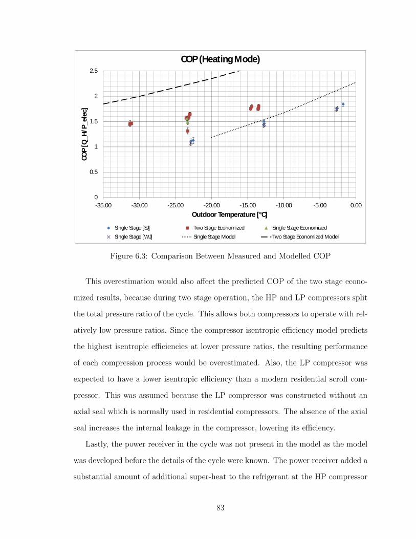
0

0.5

1

1.5

2

2.5

-35.00 -30.00 -25.00 -20.00 -15.00 -10.00 -5.00 0.00

COP

[Q_H

/P_e

lec]

Outdoor Temperature [°C]

COP (Heating Mode)

Single Stage [SJ] Two Stage Economized Single Stage Economized

Single Stage [WJ] Single Stage Model Two Stage Economized Model

Figure 6.3: Comparison Between Measured and Modelled COP

This overestimation would also affect the predicted COP of the two stage econo-

mized results, because during two stage operation, the HP and LP compressors split

the total pressure ratio of the cycle. This allows both compressors to operate with rel-

atively low pressure ratios. Since the compressor isentropic efficiency model predicts

the highest isentropic efficiencies at lower pressure ratios, the resulting performance

of each compression process would be overestimated. Also, the LP compressor was

expected to have a lower isentropic efficiency than a modern residential scroll com-

pressor. This was assumed because the LP compressor was constructed without an

axial seal which is normally used in residential compressors. The absence of the axial

seal increases the internal leakage in the compressor, lowering its efficiency.

Lastly, the power receiver in the cycle was not present in the model as the model

was developed before the details of the cycle were known. The power receiver added a

substantial amount of additional super-heat to the refrigerant at the HP compressor

83

inlet during single stage operation and at the LP compressor inlet during two stage

economized operation. Under some testing conditions, the power receiver added an

additional 30C of super-heat to the inlet vapour when compared to the modelling re-

sults. This is a significant difference in operating conditions between the experimental

apparatus and the modelling assumptions.

These differences could be accounted for if the modelling study was repeated.

However, the initial modelling results are still considered to be representative of what

would be achievable if the experimental system was designed as a whole. The cy-

cle could be constructed without the power receiver and the compressors could be

selected with isentropic efficiencies that are closer to those used during modelling.

This is also in agreement with the work of Bertsch et al. [8] whose experimental

investigation showed results that are comparable to the modelled results of the two

stage economized heat pump.

6.4 Real-World Implications

The increased COP of the two stage economized cycle reduces the energy required

to operate a heating system when compared to a single stage cycle or a backup

resistive element. This also extends the range of operation of the heat pump to

ambient temperatures below -30C. The system tested maintained a COP of 1.5 at

this temperature which represents a 50% increase in performance compared to a

resistive heating element. As well, the addition of the second stage compressor more

than doubled the heating capacity of the cycle across the operating range. This could

eliminate the need for a backup system whose capital cost could be used to partially

offset the cost of the second compressor. Therefore, the two stage economized cycle

offers more benefits than a single stage cycle in cold climate operation.

84

Although not exploited during this work because the HP compressor was much

larger than the LP compressor, both compressors were capable of variable speed op-

eration. This capability adds two major benefits to the cycle. First, the proportion of

work contributed by each compressor can be controlled at every ambient temperature

by varying their relative speeds. Second, the heating capacity can be controlled by

varying the speeds of both compressors together.

6.4.1 Optimized COP

The ability to control the intermediate pressure by varying the speed of the LP

compressor relative to the speed of HP compressor, allows the COP of the system

to be optimized at each ambient temperature. This is evident from the relationship

between the COP and the intermediate pressure outlined in Section 2.7.1 and from the

relationship between the intermediate pressure and the LP compressor speed outlined

in Section 5.1.4. This is an important factor for a real-world system as it allows the

system to operate with high performance under variable operating conditions. If fixed

speed compressors are used, the intermediate pressure would be optimized for a single

operating condition. When the system is operated under conditions other than the

design specifications, the system’s performance could be negatively effected.

6.4.2 Variable Heating Capacity

The ability to vary the speeds of both compressors together would allow the heating

capacity of the system to be varied which could increase the comfort of the user. By

matching the heating capacity to the loading on the house, the temperature fluctua-

tions within the heated space could be minimized.

85

6.5 Closing Remarks

The results of the experimental study show an increase in the COP of the heat pump

when using a two stage economized cycle versus a single stage cycle. They also show

an increase in the heating capacity of the system and an extension of the operating

range to an ambient temperature of -31C. The average data that are shown in this

chapter are shown in detail in Appendix H. The following chapter will summarize the

findings of this work and discuss areas where future work could be done.

86

Chapter 7

Conclusions and Recommendations

7.1 Conclusions and Contributions

As discussed in Chapter 1, the purpose of this work was to increase the performance

and extend the operating range of an air source heat pump to enable its use in

Canadian climates without requiring a backup heating system.

Three EES models of two stage heat pump cycles with various modifications were

compared to the performance of a traditional single stage cycle. The results indicated

that a COP of greater than 1.5 could be expected at an ambient temperature of -40C

and a supply temperature of 50C. They also indicated that the two stage economized

cycle was the best candidate for experimental work.

An experimental apparatus was constructed by modifying a Mitsubishi Zuba heat

pump to operate as a two stage economized heat pump. The system was tested in a

refrigerated container to simulate the ambient temperatures that are present in cold

climates. A COP of 1.5 was measured at an ambient temperature of -31C with a

supply temperature of 40 C.

This research has shown the benefits of using a two stage heat pump cycle for

heating in Canadian climates. This was accomplished through the successful integra-

tion of an automotive air conditioning compressor into a residential heat pump. The

addition of the second compressor extended the operating range of the heat pump

to an ambient temperature of -31C, thus demonstrating suitability for Canadian

climates without a backup heating system. This work is also evidence that existing

technologies can achieve these results if the components are integrated properly.

87

7.2 Recommendations for Future Work

This work could be continued or improved in many ways. The compressor model used

during the EES modelling investigation discussed in Chapter 2 should be updated

to a model that is a function of both inlet density and pressure ratio, rather than

pressure ratio alone. This could be accomplished using a developed model for scroll

compressors from literature or by developing a detailed relation using compressor

performance data. This would improve the accuracy of the modelled results.

A model should be developed for the experimental prototype. This would provide

an improved comparison between the modelling and experimental results as there

were differences between the physical construction of the prototype and the modelling

assumptions that were used. Any discrepancies that arise between the results of the

new model and the experimental results should be investigated. This would help to

identify areas of weakness in the modelling approach.

The isentropic efficiencies of the compressors could be calculated using the data

that were collected during the experimental work. These efficiencies could be used in

a model of the experimental prototype which would provide a better understanding

of the performance of the cycle.

Multiple refrigerants should be considered to determine if there is potential for

increased performance using a refrigerant other than R-410a. This is also important

because R-410a, along with other HFCs, may be phased out in the future.

An appropriately scaled model of the two stage economized cycle should be cre-

ated to simulate residential use of the system in Canadian climates. The model

should include compressor isentropic efficiencies from appropriate compressor data,

and realistic heat transfer models for the heat exchangers. This would provide a

better representation of the system performance and also allow simulation studies to

determine the long term performance of the system.

88

A two stage economized heat pump should be built from highest quality hardware

and software for experimental purposes. Results from testing this system would give a

better indication of the performance that can be achieved using existing compressors

and heat exchangers.

An intelligent approach to defrosting the evaporator should be developed and

studied using the experimental heat pump. This would determine the impact the

defrost cycle has on the long term performance of the heat pump.

The temperature of the heating fluid should also be varied to characterize the

affect this parameter has on the performance of the system. This would determine

the performance of the heat pump if it were used to provide heating using a method

other than forced air. For example, the COP of the heat pump could be increased by

reducing the supply temperature for use with radiant flooring.

The potential for providing domestic hot water using the heat pump should also

be studied. This could be accomplished by either increasing the supply temperature

when there is a demand for hot water, or by adding an additional heat exchanger

to provide domestic water heating using the high temperature refrigerant as it exits

the compressors. If possible, this could offset the cost of the system by removing the

need for a separate domestic hot water heating system.

Lastly, improvements at the component level should be made. Centrifugal com-

pressors and micro-channel heat exchangers could be combined to investigate the

performance of a system which uses emerging technologies.

89

References

[1] CAN/CSA-F280-M80. Determining the Required Capacity of Residential Space

Heating and Cooling Appliances. 2012.

[2] Environment Canada Historical Climate Data. http://climate.weather.gc.ca. Ac-

cessed: 2013-10-10.

[3] UNEP. Report Of The Task Force on HCFC Issues And Emissions Reduction

Benefits Arising From Earlier HCFC Phase-Out and Other Practical Measures,

journal = Montreal Protocol on Substances That Deplete The Ozone Layer,

Technology and Economic Assessment Panel. 2007.

[4] EIA. HFCs, the Montreal Protocol and the UNFCCC: Eliminating 1 of the 6

Kyoto gases. Bangkok climate change conference, 2012.

[5] A. D. Parekh and P. R. Tailor. Thermodynamic Analysis of R507A-R23 Cas-

cade Refrigeration System. International Journal of Aerospace and Mechanical

Engineering, 2012.

[6] Souvik Bhattacharyya, Anirban Garai, and Jahar Sarkar. Thermodynamic anal-

ysis and optimization of a novel N2O−CO2 cascade system for refrigeration and

heating. International Journal of Refrigeration, 32:1077–1084, 2009.

[7] Stefan S. Bertsch and Eckhard A. Groll. Air Source Heat Pump for North-

ern Climates Part I: Simulation of Different Heat Pump Cycles. International

Refrigeration and Air Conditioning Conference, Paper:783, 2006.

[8] Stefan S. Bertsch and Eckhard A. Groll. Air Source Heat Pump for Northern

Climates Part II: Measurement and Verification. International Refrigeration and

Air Conditioning Conference, Paper:784, 2006.

90

[9] Stephen Caskey, Shuai Deng, Derek Kultgen, Tobias Menzi, Eckhard Groll,

William Hutzel, and Stefan Bertsch. Field Test Simulation of an Air-Source

Heat Pump with Two-Stage Compression and Economizing For Cold Climates.

International Refrigeration and Air Conditioning Conference, Paper:2381, 2012.

[10] Tobias Menzi, Stephen Caskey, Derek Kultgen, Eckhard Groll, William Hutzel,

and Stefan Bertsch. Analysis of heating and cooling options for military barracks

in the midwest u.s. Technical report, Interstate University of Applied Sciences

of Technology NTB.

[11] Xudon Wang, Yunho Hwang, and Reinhard Radermacher. Two-stage heat pump

system with vapor-injected scroll compressor using R410A as a refrigerant. In-

ternational Journal of Refrigeration, 32:1442–1451, 2009.

[12] Kai Du, Shaoqian Zhang, Weirong Xu, and Xiaofeng Niu. A study on the cycle

characteristics of an auto-cascade refrigeration system. Experimental Thermal

and Fluid Science, 33:240–245, 2009.

[13] Brian T Austin and K Sumathy. Transcritical carbon dioxide heat pump systems:

A review. Renewable and Sustainable Energy Reviews, 15:4013–4029, 2011.

[14] Detlef Westphalen. Converting a Military Environmental Control Unit to Propy-

lene Refrigerant. International Refrigeration and Air Conditioning Conference,

Paper:840, 2006.

[15] Emerson Climate Technologies Online Product Information

and Technical Data. http://www.emersonclimate.com/en-

ca/resources/online product information/pages/online product information.aspx.

Accessed: 2014-06-10.

91

[16] J Schiffmann and D Favrat. Design, experimental investigation and multi-

objective optimization of a small-scale radial compressor for heat pump applica-

tions. Energy, 35:436–450, 2009.

[17] J Schiffmann and D Favrat. Experimental investigation of a direct driven radial

compressor for domestic heat pumps. International Journal of Refrigeration,

32:1918–1928, 2009.

[18] E. W. Lemmon. Psuedo-Pure Fluid Equations of State for the Refrigerant Blends

R-410A, R-404A, R-507A, and R-407C. International Journal of Thermophysics,

24(4):991 – 1006.

[19] Robert J Moffat. Describing the Uncertainties in Experimental Results. Experi-

mental Thermal and Fluid Science, 1988.

[20] Dow. A guide to glycols. http://www.dow.com/webapps/lit/litorder.asp?filepath=propyleneglycol/pdfs/noreg/117-

01682.pdf, 2003. Accessed: 2014-06-10.

[21] LabVIEW, PID and Fuzzy Logic Toolkit User Manual.

www.ni.com/pdf/manuals/372192d.pdf, 2009. Accessed: 2014-09-20.

92

Appendix A

EES Models

This appendix contains copies of the EES models that were used during the modelling

study that was outlined in Chapter 2.

93

File:SingleStageCycleR410aFINAL.EES 2016-01-11 08:51:43 Page 1EES Ver. 9.660: #3243: For use only by Tom Mackintosh Natural, Resources Canada

"Model #1, single compression stage (valid for single component refrigerants or azeotropic mixtures with critical temperatures >60 C)""Design Conditions"

T_supply=50T_high=T_supply+3+T_subcoolT_ambient=0T_low=T_ambient - T_superheat - 3 T_superheat=11.1 [C] "Degree of superheat at compressor inlet (Controlled by expansion valve)"T_subcool=8.3 [C] "Degree of subcooling at condensor outlet (Controlled by refrigerant charge)"R$='R410a' "Refrigerant Variable"eta_lowCompressor=(a+b*Pr+C*Pr^2)/100 "Compressor Isentropic Efficiency"a=93.7884b=-8.13742c=0.156422P_drop=1.0 "Pressure Drop Through Heat Exchangers (1.0 = Neglected)"

"Q_vap=enthalpy_vaporization(R$,T=T[2])"Q_superheat=H[2]-enthalpy(R$,p=p[2],x=1)

"State Point 1 - Compressor Inlet""Set Variables"

T[1]=T_low+T_superheat "Compressor inlet temperaturer controlled by expansion valve"P[1]=Pressure(R$,T=T_low,X=1)

"Calculated Variables"H[1]=enthalpy(R$,T=T[1],P=P[1])S[1]=entropy(R$,T=T[1],P=P[1])V[1]=volume(R$,T=T[1],P=P[1])

"State Point 2 - Compressor outlet""Set Variables"

P[2]=pressure(R$,T=T_high,X=0)/P_drop "P_drop applied to HX inlet as P_sat should remain the same.""Isentropic Conditions"

S_e2=S[1]H_e2=enthalpy(R$,S=S_e2,P=P[2])

"Calculated Variables"H[2]=H[1]+(H_e2-H[1])/eta_lowCompressor "From isentropic efficiency of compressor"S[2]=entropy(R$,H=H[2],P=P[2])T[2]=temperature(R$,H=H[2],P=P[2])V[2]=volume(R$,H=h[2],p=p[2])

"State Point 3 - Condenser Outlet" "Set Variables"P[3]=P[2]T[3]=T_high-T_subcool "Subcooling is a function of refrigerant charge (designed subcooling for system)"

"Calculated Variables"H[3]=enthalpy(R$,T=T[3],P=P[3])S[3]=entropy(R$,T=T[3],P=P[3])

"State Point 4 - Expansion Valve Outlet""Set Variables"

H[4]=H[3] "Isenthalpic expansion is most commonly used approach"P[4]=P[1]*P_drop "Pressure is determined by compressor inlet with a factor for pressure drop"

"Calculated Variables"T[4]=temperature(R$,H=H[4],P=P[4])S[4]=entropy(R$,H=H[4],P=P[4])

"State Point 5 - repeat of State 1 for closure of cycle"T[5]=T[1]

Figure A.1: Single Stage Cycle EES Model Page. 1

94

File:SingleStageCycleR410aFINAL.EES 2016-01-11 08:51:43 Page 2EES Ver. 9.660: #3243: For use only by Tom Mackintosh Natural, Resources Canada

P[5]=P[1]H[5]=H[1]S[5]=S[1]

"Energy Balance"Q_input=m[1]*(H[5]-H[4])Q_output=m[1]*(H[3]-H[2])W_input=m[1]*(H[2]-H[1])W_input=1COP_heating=abs((Q_output/W_input))COP_cooling=abs((Q_input/W_input))

"Design Requirements"Pr=P[2]/P[1] "Pressure Ratio Required for operation"Vr=V[1]/V[2]

Figure A.2: Single Stage Cycle EES Model Page. 2

95

File:2StageCascade410aFINAL.EES 2016-01-11 09:18:21 Page 1EES Ver. 9.660: #3243: For use only by Tom Mackintosh Natural, Resources Canada

"Model #2, Two Stage Cascade Cycle (valid for single component refrigerants or azeotropic mixtures with critical temperatures >60 C)""Design Conditions"

T_supply=50T_high=T_supply + 3 + T_subcool "Condensor saturation temperature"T_intermediate=-18 [C] "Intermediate Temperature, (upper cycle evaporator Temp)"T_ambient = -40T_low=T_ambient - T_superheat - 3 [C] "Evaporator saturation temperature"T_superheat=11.1 [C] "Degree of superheat at compressor inlet (Controlled by expansion valve)"T_subcool=8.3 [C] "Degree of subcooling at condensor outlet (Controlled by refrigerant charge)"RH$='r410a' "Refrigerant Variable"RL$='r410a'eta_highCompressor=0.7"(a+b*Pr_High+c*Pr_high^2)/100"a=93.7884B=-8.13742c=0.156422eta_lowCompressor=(a+b*Pr_Low+c*Pr_Low^2)/100 "Compressor Isentropic Efficiency"P_drop=1 "Pressure Drop Through Heat Exchangers (1.0 = Neglected)"

"Upper Cycle""State Point 1 - Compressor Inlet""Set Variables"T[1]=T_intermediate+T_superheat "Compressor inlet temperaturer controlled by expansion valve"P[1]=Pressure(RH$,T=T_intermediate,x=1)"Calculated Variables"H[1]=enthalpy(RH$,T=T[1],P=P[1])S[1]=entropy(RH$,T=T[1],P=P[1])

"State Point 2 - Compressor outlet""Set Variables"P[2]=Pressure(RH$,T=T_high,x=1)/P_drop "P_drop applied to HX inlet as P_sat should remain the same.""Isentropic Conditions"S_e2=S[1]H_e2=enthalpy(RH$,S=S_e2,P=P[2])"Calculated Variables"H[2]=H[1]+(H_e2-H[1])/eta_HighCompressor "From isentropic efficiency of compressor"S[2]=entropy(RH$,H=H[2],P=P[2])T[2]=temperature(RH$,H=H[2],P=P[2])

"State Point 3 - Condenser Outlet" "Set Variables"

P[3]=P[2]T[3]=T_high -T_subcool "Subcooling is a function of refrigerant charge (designed subcooling

for system)""Calculated Variables"H[3]=enthalpy(RH$,T=T[3],P=P[3])S[3]=entropy(RH$,T=T[3],P=P[3])

"State Point 4 - Expansion Valve Outlet""Set Variables"H[4]=H[3] "Isenthalpic expansion is most commonly used approach"P[4]=P[1]/P_drop "Pressure is determined by compressor inlet with a factor for

pressure drop""Calculated Variables"T[4]=temperature(RH$,H=H[4],P=P[4])S[4]=entropy(RH$,H=H[4],P=P[4])

"State Point 5 - repeat of State 1 for closure of cycle"T[5]=T[1]

Figure A.3: Two Stage Cascade Cycle EES Model Page. 1

96

File:2StageCascade410aFINAL.EES 2016-01-11 09:18:21 Page 2EES Ver. 9.660: #3243: For use only by Tom Mackintosh Natural, Resources Canada

P[5]=P[1]H[5]=H[1]S[5]=S[1]

"Energy Balance""Q_intermediate=m[1]*(H[5]-H[4])"Q_output=m[1]*(H[3]-H[2])W_high=m[1]*(H[2]-H[1])COP_High=abs((Q_output/W_high))Q_HighInput=m[1]*(H[5]-H[4])

"Design Requirements"Pr_high=P[2]/P[1] "Pressure Ratio Required for operation"

"Lower Cycle""State Point 6 - Compressor Inlet""Set Variables"T[6]=T_low+T_superheat "Compressor inlet temperaturer controlled by expansion valve"P[6]=Pressure(RL$,T=T_low,x=1)"Calculated Variables"H[6]=enthalpy(RL$,T=T[6],P=P[6])S[6]=entropy(RL$,T=T[6],P=P[6])"m[6]=m[1]*(H[5]-H[4])/(H[10]-H[9])"

"State Point 7 - Compressor outlet""Set Variables"P[7]=Pressure(RL$,T=T_intermediate+3+T_subcool,x=1)/P_drop "P_drop

applied to HX inlet as P_sat should remain the same.""Isentropic Conditions"S_e7=S[6]H_e7=enthalpy(RL$,S=S_e7,P=P[7])"Calculated Variables"H[7]=H[6]+(H_e7-H[6])/eta_lowCompressor "From isentropic efficiency of compressor"S[7]=entropy(RL$,H=H[7],P=P[7])T[7]=temperature(RL$,H=H[7],P=P[7])

"State Point 8 - Condenser Outlet" "Set Variables"

P[8]=P[7]T[8]=T_intermediate+3 "Subcooling is a function of refrigerant charge (designed subcooling

for system)"

"Calculated Variables"H[8]=enthalpy(RL$,t=t[8],p=p[8])S[8]=entropy(RL$,T=T[8],P=P[8])

"State Point 9 - Expansion Valve Outlet""Set Variables"H[9]=H[8] "Isenthalpic expansion is most commonly used approach"P[9]=P[6]/P_drop "Pressure is determined by compressor inlet with a factor for

pressure drop""Calculated Variables"T[9]=temperature(RL$,H=H[9],P=P[9])S[9]=entropy(RL$,H=H[9],P=P[9])

"State Point 10 - repeat of State 6 for closure of cycle"T[10]=T[6]P[10]=P[6]H[10]=H[6]S[10]=S[6]

"Energy Balance"Q_input=m[6]*(H[10]-H[9])

Figure A.4: Two Stage Cascade Cycle EES Model Page. 2

File:2StageCascade410aFINAL.EES 2016-01-11 09:18:21 Page 3EES Ver. 9.660: #3243: For use only by Tom Mackintosh Natural, Resources Canada

"Q_intermediate=m[6]*(H[7]-H[8])"m[6]=m[1]*(H[4]-H[5])/(H[8]-H[7])W_lowOutput=m[6]*(H[10]-H[9])W_Low=m[6]*(H[7]-H[6])W=W_low+W_high

W=1COP_Low=abs((Q_output/W_Low))COP_Heating=abs((Q_output/(W_low+W_high)))

"Design Requirements"Pr_low=P[7]/P[6] "Pressure Ratio Required for operation"

Figure A.5: Two Stage Cascade Cycle EES Model Page. 3

97

File:2StageCycleFlashSeparation.EES 2016-01-11 09:29:55 Page 1EES Ver. 9.660: #3243: For use only by Tom Mackintosh Natural, Resources Canada

"Model #1, single compression stage (valid for all refrigerants and azeotropic mixtures with critical temperatures >60 C)""Design Conditions"

T_supply=50T_high=T_supply+3+T_subcool "Condensor saturation temperature"T_ambient=-40T_low=T_ambient-T_superheat-3 "Evaporator saturation temperature""T_inj=0" "Flash tank temperature (Controlled directly)"W_input=1m[2]=m[1]-m_injT_superheat=11.1 [C] "Degree of superheat at compressor inlet (Controlled by expansion valve)"T_subcool=8.3 [C] "Degree of subcooling at condensor outlet (Controlled by refrigerant charge)"R$='r410a' "Refrigerant Variable""eta_LPComp=(a +b*Pr_LP+c*Pr_LP^2)/100"eta_LPComp=0.7a=93.7884b=-8.13742c=0.156422"eta_HPComp=(a+b*Pr_HP+c*Pr_HP^2)/100"eta_HPComp=0.7P_drop=1.0 "Pressure Drop Through Heat Exchangers"

"State Point 1 - LP Compressor Inlet""Controlled"T[1]=T_low+T_superheat "Controlled by expansion device and evap temp"

"Dependent"P[1]=pressure(R$,T=T_low,x=1)H[1]=enthalpy(R$,t=t[1],p=p[1])S[1]=entropy(R$,t=t[1],p=p[1])V[1]=volume(R$,t=t[1],p=p[1])C[1]=soundspeed(R$,T=T[1],P=P[1])

"State Point 2 LP compressor outlet""Controlled"P[2]=Pressure(R$,T=T_inj,x=1) "Controlled by intermediate pressure""Isentropic Compression"S_s2=S[1]H_s2=enthalpy(R$,P=P[2],S=s_s2)

"Dependent"H[2]=(H_s2-H[1])/eta_LPComp+H[1]T[2]=temperature(R$,p=p[2],h=h[2])S[2]=entropy(R$,p=p[2],h=h[2])

"State Point 3 HP compressor inlet""Controlled"P[3]=P[2] "Same as 2""T[3]=Temperature(R$,P=P[3],x=1)+T_superheat""Dependent""H[3]=enthalpy(R$,P=P[3],T=T[3])"H[3]=(m[2]*H[2]+m_inj*H[11])/m[1] "Ideal Mixing Process"T[3]=temperature(R$,p=p[3],h=h[3])S[3]=entropy(R$,p=p[3],h=h[3])V[3]=volume(R$,p=p[3],h=h[3])

"State Point 4 HP compressor outlet""Controlled"P[4]=pressure(R$,T=T_high,x=0) "Controlled by Condenser temp"

Figure A.6: Two Stage Flash Separation Cycle EES Model Page. 1

98

File:2StageCycleFlashSeparation.EES 2016-01-11 09:57:29 Page 2EES Ver. 9.660: #3243: For use only by Tom Mackintosh Natural, Resources Canada

"Isentropic Compression"S_s4=S[3]H_s4=enthalpy(R$,P=P[4],S=S_s4)

"Dependent"H[4]=(H_s4-H[3])/eta_HPComp+H[3]T[4]=temperature(R$,p=p[4],h=h[4])S[4]=entropy(R$,p=p[4],h=h[4])

"State point 5 Condenser Outlet""Controlled"T[5]=T_high-t_subcool "Controlled by refrigerant charge, condensor temp"

"Dependent"P[5]=P[4]H[5]=enthalpy(R$,t=t[5],P=P[5])S[5]=entropy(R$,t=t[5],p=p[5])

"State point 6 Flash tank inlet""Controlled"H[6]=H[5] "Constant enthalpy expansion"m_inj=m[1]*(quality(R$,P=P[6],H=h[6]))"T[6]=T_inj""Dependent""P[6]=Pressure(R$,H=H[6],T=T[6])"P[6]=Pressure(R$,t=T_inj,x=1)T[6]=temperature(R$,p=p[6],h=h[6])S[6]=entropy(R$,p=p[6],h=h[6])

"State point 7 liquid stream outlet"P[7]=P[6]X[7]=0

"dependent"H[7]=enthalpy(R$,p=p[7],x=x[7])S[7]=entropy(R$,p=p[7],x=x[7])T[7]=temperature(R$,p=p[7],x=x[7])

"State Point 8 Evaporator inlet"P[8]=P[1]H[8]=H[7] "Constant Enthalpy expansion"

"dependent"T[8]=temperature(R$,p=p[8],h=h[8])S[8]=entropy(R$,p=p[8],h=h[8])

"State Point 9 Repeat of 1"P[9]=p[1]H[9]=h[1]T[9]=t[1]S[9]=S[1]

"State point 10 Repeat of 6"P[10]=p[6]H[10]=h[6]T[10]=t[6]S[10]=s[6]

"State Point 11 Vapor stream tank outlet"P[11]=P[10]X[11]=1

"Dependent"

Figure A.7: Two Stage Flash Separation Cycle EES Model Page. 2

99

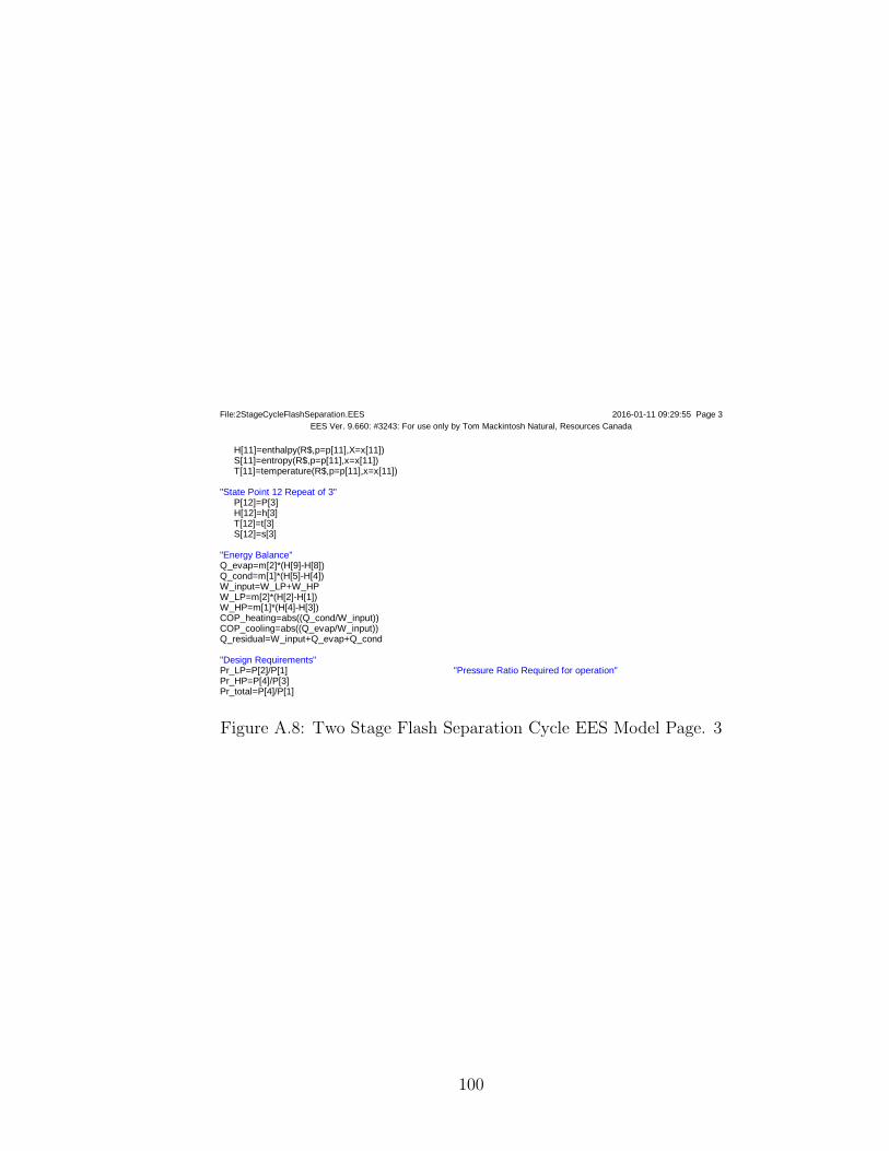
File:2StageCycleFlashSeparation.EES 2016-01-11 09:29:55 Page 3EES Ver. 9.660: #3243: For use only by Tom Mackintosh Natural, Resources Canada

H[11]=enthalpy(R$,p=p[11],X=x[11])S[11]=entropy(R$,p=p[11],x=x[11])T[11]=temperature(R$,p=p[11],x=x[11])

"State Point 12 Repeat of 3"P[12]=P[3]H[12]=h[3]T[12]=t[3]S[12]=s[3]

"Energy Balance"Q_evap=m[2]*(H[9]-H[8])Q_cond=m[1]*(H[5]-H[4])W_input=W_LP+W_HPW_LP=m[2]*(H[2]-H[1])W_HP=m[1]*(H[4]-H[3])COP_heating=abs((Q_cond/W_input))COP_cooling=abs((Q_evap/W_input))Q_residual=W_input+Q_evap+Q_cond

"Design Requirements"Pr_LP=P[2]/P[1] "Pressure Ratio Required for operation"Pr_HP=P[4]/P[3]Pr_total=P[4]/P[1]

Figure A.8: Two Stage Flash Separation Cycle EES Model Page. 3

100

File:2StageCycleEconomizing410aFINAL_Updated.EES 2016-01-11 09:47:48 Page 1EES Ver. 9.660: #3243: For use only by Tom Mackintosh Natural, Resources Canada

"Model #1, single compression stage (valid for all refrigerants with critical temperatures >60 C)""Design Conditions"ErrorCheck=T[7]-T[11]

T_supply=50T_high=T_supply + 3 + T_subcool "Condensor saturation temperature"T_ambient=0T_low=T_ambient-T_superheat-3 "Evaporator saturation temperature"T_inj=21 "Flash tank temperature (Controlled directly)"m[1]=0.01688 [kg/s] "Mass flow rate"m_inj=m[1]*X_injX_inj=0.321m[2]=m[1]-m_inj

T_superheat=11.1 [C] "Degree of superheat at compressor inlet (Controlled by expansion valve)"T_subcool=8.3 [C] "Degree of subcooling at condensor outlet (Controlled by refrigerant charge)"R$='r410a' "Refrigerant Variable""eta_LPComp=(a +b*Pr_LP+c*Pr_LP^2)/100" "Compressor Isentropic Efficiency"eta_LPComp=0.7a=93.7884b=-8.13742c=0.156422"eta_HPComp=(a+b*Pr_HP+c*Pr_HP^2)/100"eta_HPComp=0.7P_drop=1.0 "Pressure Drop Through Heat Exchangers"

"State Point 1 - LP Compressor Inlet""Controlled"T[1]=T_low+T_superheat "Controlled by expansion device and evap temp"

"Dependent"P[1]=(0.5)*(pressure(R$,T=t_low,X=1)+pressure(R$,T=T_low,x=0))H[1]=enthalpy(R$,t=t[1],p=p[1])S[1]=entropy(R$,t=t[1],p=p[1])V[1]=volume(R$,t=t[1],p=p[1])C[1]=soundspeed(R$,T=T[1],P=P[1])

"State Point 2 LP compressor outlet""Controlled"P[2]=Pressure(R$,T=T_inj,x=1) "Controlled by intermediate pressure""Isentropic Compression"S_s2=S[1]H_s2=enthalpy(R$,P=P[2],S=s_s2)

"Dependent"H[2]=(H_s2-H[1])/eta_LPComp+H[1]T[2]=temperature(R$,p=p[2],h=h[2])S[2]=entropy(R$,p=p[2],h=h[2])

"State Point 3 HP compressor inlet""Controlled"P[3]=P[2] "Same as 2"

"Dependent"H[3]=(m[2]*H[2]+m_inj*H[12])/m[1] "Ideal Mixing Process""T[3]=temperature(R$,p=p[3],h=h[3])"H[3]=enthalpy(R$,P=P[3],T=T[3])

Figure A.9: Two Stage Economized Cycle EES Model Page. 1

101

File:2StageCycleEconomizing410aFINAL_Updated.EES 2016-01-11 09:47:48 Page 2EES Ver. 9.660: #3243: For use only by Tom Mackintosh Natural, Resources Canada

T[3]=temperature(R$,P=P[3],X=1)+T_superheatS[3]=entropy(R$,p=p[3],h=h[3])V[3]=volume(R$,p=p[3],h=h[3])

"State Point 4 HP compressor outlet""Controlled"P[4]=(0.5)*(pressure(R$,T=t_high,X=1)+pressure(R$,T=T_high,x=0)) "Controlled by

Condenser temp"

"Isentropic Compression"S_s4=S[3]H_s4=enthalpy(R$,P=P[4],S=S_s4)

"Dependent"H[4]=(H_s4-H[3])/eta_HPComp+H[3]T[4]=temperature(R$,p=p[4],h=h[4])S[4]=entropy(R$,p=p[4],h=h[4])

"State point 5 Condenser Outlet""Controlled"T[5]=T_high-t_subcool "Controlled by refrigerant charge, condensor temp"

"Dependent"P[5]=P[4]H[5]=enthalpy(R$,t=t[5],P=P[5])S[5]=entropy(R$,t=t[5],p=p[5])

"State point 6 Receiver outlet"P[6]=P[5]H[6]=H[5]"dependent"

S[6]=entropy(R$,p=p[6],h=H[6])T[6]=temperature(R$,p=p[6],h=H[6])

"State point 7 Main Econo Out""Controlled"H[7]=(m_inj*(H[11]-H[12])/m[2])+H[6]

"Dependent"P[7]=P[4]T[7]=temperature(R$,p=p[7],h=h[7])S[7]=entropy(R$,p=p[7],h=h[7])

"State Point 8 Evaporator inlet"P[8]=P[1]H[8]=H[7] "Constant Enthalpy expansion"

"dependent"T[8]=temperature(R$,p=p[8],h=h[8])S[8]=entropy(R$,p=p[8],h=h[8])

"State Point 9 Repeat of 1"P[9]=p[1]H[9]=h[1]T[9]=t[1]S[9]=S[1]

"State point 10 Repeat of 6"P[10]=p[6]H[10]=h[6]

Figure A.10: Two Stage Economized Cycle EES Model Page. 2

102

File:2StageCycleEconomizing410aFINAL_Updated.EES 2016-01-11 09:47:48 Page 3EES Ver. 9.660: #3243: For use only by Tom Mackintosh Natural, Resources Canada

T[10]=t[6]S[10]=s[6]

"State Point 11 Econo Inlet"P[11]=P[3]H[11]=H[6]

"Dependent"S[11]=entropy(R$,p=p[11],H=H[11])T[11]=temperature(R$,p=p[11],H=H[11])

"State Point 12 Repeat of 3"P[12]=P[3]"H[12]=h[3]"T[12]=temperature(R$,P=P[12],H=H[12])S[12]=entropy(R$,P=P[12],H=H[12])

"State Point 13 Repeat of 3"P[13]=P[3]H[13]=h[3]T[13]=t[3]S[13]=s[3]

"Energy Balance"Q_evap=m[2]*(H[9]-H[8])Q_cond=m[1]*(H[5]-H[4])W_input=W_LP+W_HPW_LP=m[2]*(H[2]-H[1])W_HP=m[1]*(H[4]-H[3])COP_heating=abs((Q_cond/W_input))COP_cooling=abs((Q_evap/W_input))Q_residual=W_input+Q_evap+Q_cond

"Design Requirements"Pr_LP=P[2]/P[1] "Pressure Ratio Required for operation"Pr_HP=P[4]/P[3]Pr_total=P[4]/P[1]

Figure A.11: Two Stage Economized Cycle EES Model Page. 3

103

Appendix B

FPGA

This appendix outlines the basic function of a field programmable gate array that

was used during the experimental work.

B.1 FPGA Function

A FPGA is a reconfigurable piece of hardware that allows for rapid prototyping of

integrated circuits. It is constructed using an array of logic gates that are intercon-

nected by a variety of switching elements. The switching elements are programed to

link the logic gates in a configuration which provides the required function. Figure

B.1 shows the basic building block that is used to construct a FPGA chip.

These building blocks are connected to provide millions of gates within a single

FPGA chip. The NI cRIO-9074 controller that was used contained a Xilinx Spartan

3 FPGA which was constructed with 2 million gates.

The FPGA is configured using a machine code that is specific to the chip which

is used. LabVIEW simplifies this process by allowing the user to program the FPGA

using the same block diagram interface that is used in to program regular LabVIEW

applications, with a reduced set of tools. The program is then compiled to machine

code using a compiler.

The main benefit of using the FPGA in a LabVIEW controller is how it functions.

Normally, a software function is placed into a real-time application that is deployed to

the controller. This application runs in the operating system and is subjected to the

processor’s speed and the processor and memory queues. The FPGA functions much

104

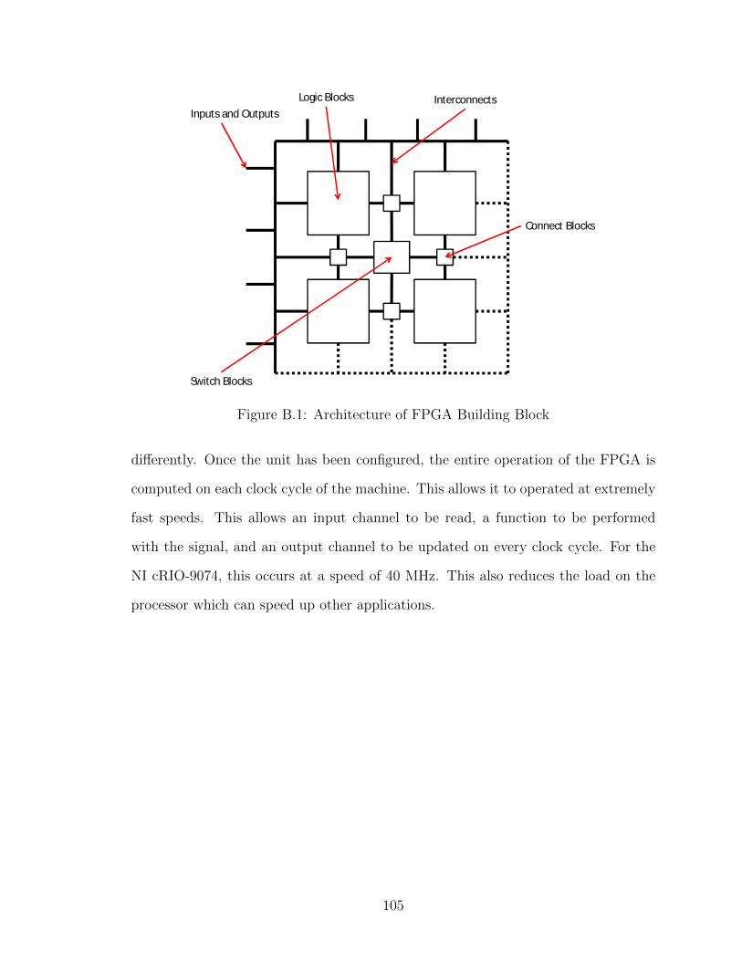
Inputs and OutputsLogic Blocks

Switch Blocks

Connect Blocks

Interconnects

Figure B.1: Architecture of FPGA Building Block

differently. Once the unit has been configured, the entire operation of the FPGA is

computed on each clock cycle of the machine. This allows it to operated at extremely

fast speeds. This allows an input channel to be read, a function to be performed

with the signal, and an output channel to be updated on every clock cycle. For the

NI cRIO-9074, this occurs at a speed of 40 MHz. This also reduces the load on the

processor which can speed up other applications.

105

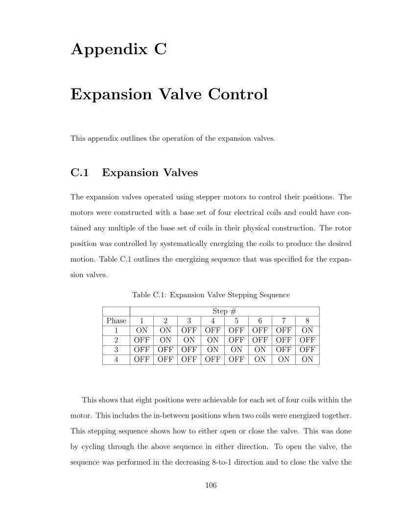
Appendix C

Expansion Valve Control

This appendix outlines the operation of the expansion valves.

C.1 Expansion Valves

The expansion valves operated using stepper motors to control their positions. The

motors were constructed with a base set of four electrical coils and could have con-

tained any multiple of the base set of coils in their physical construction. The rotor

position was controlled by systematically energizing the coils to produce the desired

motion. Table C.1 outlines the energizing sequence that was specified for the expan-

sion valves.

Table C.1: Expansion Valve Stepping Sequence

Step #Phase 1 2 3 4 5 6 7 8

1 ON ON OFF OFF OFF OFF OFF ON2 OFF ON ON ON OFF OFF OFF OFF3 OFF OFF OFF ON ON ON OFF OFF4 OFF OFF OFF OFF OFF ON ON ON

This shows that eight positions were achievable for each set of four coils within the

motor. This includes the in-between positions when two coils were energized together.

This stepping sequence shows how to either open or close the valve. This was done

by cycling through the above sequence in either direction. To open the valve, the

sequence was performed in the decreasing 8-to-1 direction and to close the valve the

106

sequence was performed in the increasing 1-to-8 direction. A total of five hundred

steps were required to move the valve from fully closed to fully opened.

To control the position, a FPGA code was written in LabVIEW which accepted a

numeric position from a higher level real-time software outlined in Appendix G. The

numeric position was intended to indicate the desired position of the valve and could

have had a value of 0 - 500. The FPGA monitored this parameter and output the

sequence that was required to move the valve to the desired position. For example, if

the position parameter was changed from 100 to 125, the FPGA would make 25 steps

in the correct direction. Figure C.1 outlines the operation of the FPGA software.

Figure C.1: Expansion Valve FPGA Software Operation

The FPGA was configured to control the NI-9401 digital output modules of the

controller. With this approach, each digital output channel directly controlled a phase

of the stepper motor.

107

The digital output module was only capable of supplying a maximum of 1 mA

of current and the stepper motor windings required 350 mA. To operate the stepper

motor, a current driving circuit was designed using the ULN2003AN integrated cir-

cuit (IC) to increase the current supplied to the coils. This IC incorporates seven

Darlington circuits into a single chip. A Darlington circuit is constructed by placing

two transistors together so that the emitter of the first is connected to the base of the

second, assuming NPN transistors are used. Since the current delivered to the emit-

ter of a transistor is a function of the current supplied to its base, the small current

delivered by the NI module is increased in the first transistor. Then the increased

current is multiplied again in the second transistor. Typical emitter currents can be

20 to 200 times greater than the base current. The Darlington circuit takes advantage

of this twice which allows the small 1 mA output to control up to 500 mA. Figure

C.2 shows the current driving circuit that was used.

12 Vdc

FromDigitalOutput

ULN2003AN

Stepper Motor

Figure C.2: Expansion Valve Current Driving Circuit (Showing OneInternal Darlington)

108

Using this approach, the high level PID algorithm, outlined in Appendix G, was

used to control the desired position of the valve, and the FPGA code would control

the operation of the coils in the stepper motor. When the software was initialized,

the valve position was calibrated by supplying 700 steps in the closed direction and

setting the position parameter to zero. This forced the motor to lock when the valve

closed and set the position reference to match the closed position. It is possible that

over time the position reference could drift from the real position of the valve. In

practice, the valve position would be calibrated at some frequency to minimize this

effect. For this work, the valves were calibrated daily as part of the startup procedure

and no effects of drift were observed during operation.

109

Appendix D

Fans

This appendix will describe the operation of the fans which were located in the out-

door unit.

D.1 Fans

The fans in the outdoor unit were originally controlled by the heat pump control

board. There are two separate fans which are each variable speed and were controlled

individually. To simplify the modifications, both fans were wired in parallel.

The fans were originally wired to the heat pump control board using a seven pin

connector. The function of the pins of this connector were determined by monitoring

the electrical signals present when the heat pump control board was powered. The

results of this are shown in Table D.1.

Table D.1: Outdoor Unit Fan Pinout

Pin Description

1 280 Vdc, Main power supply for fans2 No connection3 No connection4 Common5 15 Vdc, Logic level power supply6 0 - 6.5 Vdc, Variable speed control7 0 - 15 Vdc Pulse, Tachometer Signal

110

This shows that 3 separate direct current power signals were measured. It was

assumed that the 280 Vdc signal was the main power supply for the motors and the

15 Vdc signal was the power supply for the internal electronics within the motor.

The 0 - 6.5 Vdc signal was assumed to be the input which controlled the speed of the

motor.

For the 280 Vdc power supply, a rectifier circuit was constructed which operated

from a 208 Vac line to line power supply. The rectifier circuit used a GBJ2508-BP 25

A bridge rectifier with a 470 µF capacitor that was used to filter the voltage ripple on

the output. Due to the size of the capacitor, a 100 kΩ resistor was placed across the

output terminals to ensure that the capacitor would discharge within five minutes of

the input power being disconnected. This was done to reduce the danger of working

on the electrical system after it was installed. Figure D.1 shows the schematic of the

rectifier circuit.

Figure D.1: DC Rectifier Circuit

The 15 Vdc and 0 to 6.5 Vdc were powered via a Sorenson dual channel dc power

supply. As this equipment was available, it was the simplest approach to finish the

circuit for the fans. The tachometer signal was ignored for simplicity.

111

Appendix E

Software

This appendix will outline the architecture and general operation of the control soft-

ware.

E.1 Architecture

The software was distributed across three pieces of hardware in four applications.

This included a desktop computer, two embedded real-time controllers, and a FPGA

layer within one of the controllers. Figure E.1 outlines this distribution.

E.1.1 Desktop PC

The desktop computer operated the main user interface and provided the location

where data were stored. The graphical user interface (GUI) is shown in Figure E.2

The GUI was used to configure and provide feedback from the system during

operation. A detailed diagram of the refrigeration cycle was included which displayed

real-time data from the instrumentation. The compressor speeds, super-heat setting,

pump speed, and valve positions were controlled using inputs on this diagram. The

data logging location and interval were also configured using this interface.

E.1.2 Main Controller

The main controller was configured to read the measured values from the instrumen-

tation and to convert their readings to the desired units using the calibrated scales.

112

Figure E.1: System Software Architecture

The data were then published to the network to be recorded in the desktop PC.

The main controller also operated the super-heat control algorithm as outlined in

Appendix G. The output of this algorithm was then sent to the FPGA.

E.1.2.1 FPGA

The FPGA was used to control the position of the expansion valves. The operation

of this is described in Appendices B and C.

113

GUI.viC:\LabVIEW Projects\LabVIEW Tom\Cold Climate HP\GUI.viLast modified on 2015-02-02 at 14:20Printed on 2015-11-02 at 10:07

Page 1

file path (d ialog if empty)Record Data

40

Controlled Supply Temperature

8

Superheat Control

Sol-2

Sol-3

4 Way

Auto Superheat Control

500

Manual Valve A Setting

0

T_water_inlet

0

T_water_outlet

0

T_LP_inlet

0

T_LP_outlet

0

T_HP_inlet

0

T_HP_outlet

0

T_Cond_outlet

0

T_receiver_outlet

0

T_Econo_outlet

0

T_LEVa_outlet

0

T_Evap_outlet

0

T_inj_LEV_outlet

0

T_inj_Econo_outlet

0

T _Am bi e nt

Circulation Pump On

0

Manual Valve BCalibrate Expansion Valves

0

P_evap

0

P_inject

0

P_cond

460

Manual Valve C

0

Volume Flow Rate GPM

LP Compressor Run

HP Compressor Run

0

LP Speed V

3.71

HP Speed V

0

SaturationTemp

0

CondSaturation T e m p

0

InjectSaturationTemp

0

Heat Delivered

0

HP Powe r

0

LP Power

0

HP Hz

0

Degrees Superheat

0

Degrees Subcooling

0

LEV-A Position

0

0

0

0

0

0

0

0

0

0

0

HP VFD Output A

0

0

0

0

0

0

Ch 4 A

0

0

0

0

0

0

Ch 4 B

0

0

0

0

0

0

0

0

0

0

0

LP VFD A

Compressor Power

0

0

0

0

0

0

0

0

0

0

0

HP VFD Output B

Voltage

Current

VA

W

PF

Frequency

0

0

0

0

0

0

0

0

0

0

0

LP VFD B

Voltage

Current

VA

W

PF

Frequency

0

L P Am ps

0

LP HzMaster Alarm

Reset Alarm

Arm Master A l arm

Auto Start

0

Wait Time Before AutoStart (s)

Armed

Reset

O n

O n

O n

0

0

0

0

0

0

0

0

0

0

0

HP VFD Output C

0

0

0

0

0

0

0

0

0

0

0

LP VFD C

Vf

Af

Wf

VAf

PFf

Vf

Af

Wf

VAf

PFf

0

DT/Dt (min)

0

Superheat

Figure E.2: System Graphical User Interface

E.1.3 Hydronics Controller

The hydronics controller was used to control the heat dump outlined in Section 3.3.7.

It operated a PID control algorithm which controlled the supply temperature to the

condenser by varying the fan speed of the heat dump. The flow rate measurement

was also performed by this controller as it was located closer to the flow meter than

the main controller.

E.1.4 PA-4000

The power analyzers were connected to the network which allowed their measurements

to be recorded directly on the Desktop PC.

114

Appendix F

Uncertainty

This appendix contains the uncertainties that were calculated for each of the test

points using the procedure outlined in Chapter 4.

F.1 PA-4000 Additional Terms

The PA-4000 power analyzers were configured to the 200 V, 50 A, and 45 Hz to 850

Hz ranges during testing. According to the manual, the corresponding terms from

Equation 4.7 are shown in Table F.1.

Table F.1: PA-4000 Bias Error Terms

Vrmsacc ±0.04% of reading ±0.04% of range ±0.02 VArmsacc ±0.04% of reading ±0.04% of range ±(20 µV/Zext)Zext 9.375 mΩV h1pherr ±0.025 ±[0.005 ∗ (Vrms/Vrange)]± (0.05/Vrange)± (0.001F )Ah1pherr ±0.025 ±[0.005 ∗ (Arms/Arange)]± (0.0001/Arange ∗ Zext)± (0.001F )

where Zext is the impedance of the current shunt, Vrange is the voltage range of the

analyzer, Arange is the current range of the analyzer, and F is the measured frequency

of the first voltage harmonic.

115

F.2 Uncertainty

The uncertainties given in the plots from Chapter 6 were calculated as outlined in

Chapter 4. The values used to compute the uncertainty of the derived quantities for

each data point are given in Figures F.1 and F.2.

Data Pt# T_delta Cp Density P_in kW Q_outputB_SPRT B_Readout B_RTD B_j B_j B_meter B_NI_Gain B_BI_Offset B_j B_j B_j B_j Theta_V

1 0.011 0.009 0.021 0.025 0.036 0.003 0.000 0.000 0.003 0.006 0.003 0.004 10.1802 0.011 0.009 0.021 0.025 0.036 0.003 0.000 0.000 0.003 0.006 0.003 0.004 7.9623 0.011 0.009 0.021 0.025 0.036 0.003 0.000 0.000 0.003 0.006 0.003 0.004 5.6464 0.011 0.009 0.021 0.025 0.036 0.003 0.000 0.000 0.003 0.006 0.003 0.004 8.6095 0.011 0.009 0.021 0.025 0.036 0.003 0.000 0.000 0.003 0.006 0.003 0.004 9.2626 0.011 0.009 0.021 0.025 0.036 0.003 0.000 0.000 0.003 0.006 0.003 0.002 12.5737 0.011 0.009 0.021 0.025 0.036 0.003 0.000 0.000 0.003 0.006 0.003 0.002 12.3248 0.011 0.009 0.021 0.025 0.036 0.003 0.000 0.000 0.003 0.006 0.003 0.003 11.8779 0.011 0.009 0.021 0.025 0.036 0.003 0.000 0.000 0.003 0.006 0.003 0.002 14.732

10 0.011 0.009 0.021 0.025 0.036 0.003 0.000 0.000 0.003 0.006 0.003 0.002 12.71211 0.011 0.009 0.021 0.025 0.036 0.003 0.000 0.000 0.003 0.006 0.003 0.003 15.92812 0.011 0.009 0.021 0.025 0.036 0.003 0.000 0.000 0.003 0.006 0.003 0.002 13.43013 0.011 0.009 0.021 0.025 0.036 0.003 0.000 0.000 0.003 0.006 0.003 0.003 14.77314 0.011 0.009 0.021 0.025 0.036 0.003 0.000 0.000 0.003 0.006 0.003 0.002 11.30515 0.011 0.009 0.021 0.025 0.036 0.003 0.000 0.000 0.003 0.006 0.003 0.002 7.70716 0.011 0.009 0.021 0.025 0.036 0.003 0.000 0.000 0.003 0.006 0.003 0.003 12.62917 0.011 0.009 0.021 0.025 0.036 0.003 0.000 0.000 0.003 0.006 0.003 0.002 9.71318 0.011 0.009 0.021 0.025 0.036 0.003 0.000 0.000 0.003 0.006 0.003 0.002 7.60419 0.011 0.009 0.021 0.025 0.036 0.003 0.000 0.000 0.003 0.006 0.003 0.002 5.74620 0.011 0.009 0.021 0.025 0.036 0.003 0.000 0.000 0.003 0.006 0.003 0.001 8.07121 0.011 0.009 0.021 0.025 0.036 0.003 0.000 0.000 0.003 0.006 0.003 0.001 6.43222 0.011 0.009 0.021 0.025 0.036 0.003 0.000 0.000 0.003 0.006 0.003 0.001 4.54023 0.011 0.009 0.021 0.025 0.036 0.003 0.000 0.000 0.003 0.006 0.003 0.002 7.37724 0.011 0.009 0.021 0.025 0.036 0.003 0.000 0.000 0.003 0.006 0.003 0.002 12.46025 0.011 0.009 0.021 0.025 0.036 0.003 0.000 0.000 0.003 0.006 0.003 0.002 12.50526 0.011 0.009 0.021 0.025 0.036 0.003 0.000 0.000 0.003 0.006 0.003 0.002 10.888

T_water_outlet/Inlet Sparling

Figure F.1: Details of Uncertainty Analysis - 1

116

Q_output cont.. COPTheta_T_Delta Theta_Cp Theta_Density B_T S_hat t U_hat +/- Error % Theta_Pin Theta_Q B_T S_hat t U_hat +/- Error %

1.434 0.889 3.565 0.059 0.001 1.960 0.070 1.955 0.947 0.514 0.031 0.000 1.960 0.040 2.1771.434 0.695 2.787 0.056 0.002 1.960 0.082 2.906 0.808 0.537 0.030 0.001 1.960 0.047 3.1401.432 0.492 1.975 0.054 0.001 1.960 0.072 3.640 0.625 0.561 0.030 0.001 1.960 0.045 4.0521.437 0.753 3.021 0.057 0.001 1.960 0.074 2.442 0.733 0.491 0.028 0.000 1.960 0.042 2.8221.437 0.811 3.251 0.058 0.001 1.960 0.071 2.175 0.745 0.477 0.028 0.000 1.960 0.039 2.4681.439 1.102 4.418 0.063 0.001 1.960 0.073 1.645 0.687 0.393 0.025 0.000 1.960 0.036 2.0441.426 1.070 4.290 0.062 0.001 1.960 0.078 1.815 0.576 0.365 0.023 0.000 1.960 0.034 2.1841.428 1.033 4.142 0.062 0.001 1.960 0.070 1.671 0.514 0.351 0.022 0.000 1.960 0.029 2.0101.434 1.286 5.157 0.067 0.001 1.960 0.082 1.577 0.628 0.348 0.023 0.001 1.960 0.041 2.2521.433 1.109 4.447 0.063 0.001 1.960 0.072 1.611 0.694 0.394 0.025 0.000 1.960 0.035 1.9851.434 1.391 5.578 0.069 0.001 1.960 0.082 1.461 0.575 0.320 0.022 0.001 1.960 0.040 2.2211.434 1.172 4.702 0.065 0.001 1.960 0.079 1.679 0.573 0.348 0.023 0.000 1.960 0.036 2.2151.434 1.290 5.172 0.067 0.001 1.960 0.076 1.462 0.523 0.317 0.021 0.000 1.960 0.032 1.9561.432 0.986 3.954 0.061 0.001 1.960 0.075 1.875 0.620 0.395 0.024 0.000 1.960 0.037 2.3541.431 0.672 2.694 0.056 0.003 1.960 0.095 3.501 0.638 0.485 0.027 0.002 1.960 0.062 4.6841.435 1.103 4.424 0.063 0.001 1.960 0.073 1.629 0.479 0.328 0.021 0.001 1.960 0.057 3.8661.434 0.848 3.402 0.059 0.001 1.960 0.068 1.976 0.908 0.515 0.030 0.000 1.960 0.039 2.1921.434 0.664 2.662 0.056 0.002 1.960 0.087 3.260 0.769 0.536 0.030 0.001 1.960 0.055 3.8621.432 0.501 2.009 0.054 0.003 1.960 0.090 4.469 0.630 0.558 0.030 0.001 1.960 0.062 5.4521.427 0.701 2.812 0.056 0.001 1.960 0.065 2.306 1.069 0.614 0.035 0.000 1.960 0.043 2.4791.427 0.559 2.241 0.054 0.001 1.960 0.068 3.015 0.923 0.640 0.035 0.000 1.960 0.046 3.1981.426 0.394 1.581 0.053 0.001 1.960 0.065 4.115 0.726 0.675 0.036 0.001 1.960 0.048 4.4471.428 0.642 2.573 0.056 0.001 1.960 0.066 2.532 0.850 0.573 0.032 0.000 1.960 0.040 2.6841.429 1.084 4.347 0.063 0.001 1.960 0.077 1.748 0.703 0.401 0.025 0.000 1.960 0.036 2.0371.430 1.089 4.366 0.063 0.001 1.960 0.077 1.761 0.575 0.362 0.023 0.001 1.960 0.044 2.7901.430 0.948 3.801 0.060 0.001 1.960 0.075 1.948 0.545 0.377 0.023 0.000 1.960 0.033 2.307

Figure F.2: Details of Uncertainty Analysis - 2

117

Appendix G

Super-heat Algorithm

This appendix outlines the operation of the algorithm that was used to control the

amount of super-heat that was present in the refrigerant at the evaporator outlet,

shown as state point (9) in Figure 5.1d, by controlling the position of the heating

expansion valve.

G.1 Super-heat Defined

The super-heat at state point (9) is defined in Equation 5.1 which is shown below for

convenience.

Tsuper−heat = Tevapoutlet − Tevapsaturation

where, Tsuper−heat is the amount of super-heat that is present in the refrigerant at the

outlet of the evaporator, Tevapoutlet is the refrigerant temperature at state point (9),

as shown in Figure 5.1d, and Tevapsaturation is the refrigerant saturation temperature

that corresponds to the evaporator pressure.

This is the main controlled parameter in all heat pumps and air conditioners. This

parameter is used to prevent liquid from entering the compressor by ensuring that

the state of the refrigerant at the compressor inlet is a super-heated gas.

118

G.2 PID Algorithm

The super-heat algorithm functioned using a standard proportional-integral-derivative

(PID) feedback system that was included in LabVIEW. The PID equation is outlined

in Equation G.1.

U(t) = Kc

e+

1

Ti

∫ t

0

edt+ Tdde

dt

(G.1)

where Kc is the proportional gain, Ti is the integral time constant, Td is the derivative

time constant, and e is the error calculated using Equation G.2.

e = SP − PV (G.2)

where, SP is the super-heat set-point of 8C and PV is the process variable Tsuper−heat

from Equation 5.1.

The output of Equation G.1 was limited to a range of 0 to 500 which directly

corresponded to the position of the heating expansion valve.

The constants required in Equation G.1 were determined by performing an open

loop tuning procedure which was described in the reference manual for the LabVIEW

PID Toolkit [21]. This was accomplished by recording the parameter Tsuper−heat with

the system operating under steady condition, and manually changing the heating

expansion valve position to observe the system response. The resulting dataset was

analyzed to obtain the parameters that are outlined in Figure G.1.

where ∆n is the change in the controlled parameter, td is the system lag time, and

T is the time required for the process variable to reach 63.2% of its final value. For

this process all of the time parameters are measured with units of minutes. Lastly,

the system gain is calculated using Equation G.3.

K =∆Tsuper−heat

∆n(G.3)

119

td

Min

Max

63.2% (Max – Min)

T

ControlledParameter

ProcessVariable

Δn

Figure G.1: Super-heat Open Loop Step Response

where ∆Tsuper−heat is the change in the process variable from Min to 63.2%(Max-

Min) as shown in Figure G.1. Table G.1 shows the corresponding values that were

measured.

Table G.1: Measured Open Loop Response Parameters

∆n 6∆Tsuper−heat 8.3CK 1.383td 0.167 [min]T 0.583 [min]

The tuning parameters in Equation G.1 were calculated using Equations G.4, G.5

and G.6. Which were taken from the closed-loop-quarter-decay response table from

the LabVIEW manual [21].

Kc = 100KtdT

= 39.6 (G.4)

Ti = 2.00td = 0.334 (G.5)

120

Td = 0.50td = 0.084 (G.6)

121

Appendix H

Data

The data collected were used to produce a total of twenty six data points. This

appendix includes the averaged data that were used for analysis.

H.1 Data Points

Figure H.1 shows the legend for the data points that were collected.

The average values that were used to determine the performance of the system

for each of these data points are shown in Figure H.2. The highlighted fan power

values were not measured during testing and were added based on the later measured

values.

122

Data Point # Date Tested System Configuration Ambient Temperature [C]1 December 15, 2014 Single Stage -1.772 December 15, 2014 Single Stage -12.753 December 15, 2014 Single Stage -22.854 December 15, 2014 Single Stage Economized -23.315 December 15, 2014 Single Stage Economized -23.396 December 16, 2014 Two Stage Economized -13.567 December 16, 2014 Two Stage Economized -23.258 December 16, 2014 Two Stage Economized -31.079 December 17, 2014 Two Stage Economized -13.47

10 December 17, 2014 Two Stage Economized -13.4911 December 17, 2014 Two Stage Economized -14.4412 December 18, 2014 Two Stage Economized -23.0213 December 18, 2014 Two Stage Economized -22.9814 December 18, 2014 Two Stage Economized -23.5215 December 18, 2014 Two Stage Economized -23.3016 December 18, 2014 Two Stage Economized -31.2917 December 30, 2014 Single Stage -2.5718 December 30, 2014 Single Stage -12.7919 December 30, 2014 Single Stage -22.5320 January 20, 2015 Single Stage [WJ] -2.7221 January 20, 2015 Single Stage [WJ] -12.6822 January 20, 2015 Single Stage [WJ] -22.9023 January 20, 2015 Single Stage Economized [WJ] -23.3024 January 22, 2015 Two Stage Economized [WJ] -14.5925 January 22, 2015 Two Stage Economized [WJ] -23.1326 January 22, 2015 Two Stage Economized [WJ] -31.32

Figure H.1: Data Point Legend

123

Data

pt #

Delta

T W

ater

Volu

me

Flow

m^3

/sM

ass F

low

kg/

sQ

Del

iver

ed k

J/s

Mits

u Po

wer

kW

Dens

o Po

wer

kW

Fan

Pow

er k

WCO

P1

2.50

0.35

0.36

3.59

1.66

0.00

0.29

1.84

21.

960.

350.

352.

811.

570.

000.

291.

513

1.39

0.35

0.35

1.99

1.49

0.00

0.29

1.11

42.

120.

350.

363.

041.

750.

000.

291.

495

2.28

0.35

0.36

3.27

1.81

0.00

0.29

1.56

63.

090.

350.

364.

451.

610.

640.

291.

757

3.03

0.35

0.35

4.32

1.61

0.84

0.29

1.58

82.

920.

350.

354.

171.

610.

950.

291.

469

3.62

0.35

0.35

5.19

1.63

0.95

0.29

1.81

103.

130.

350.

354.

481.

610.

640.

291.

7611

3.92

0.35

0.36

5.62

1.65

1.18

0.29

1.80

123.

300.

350.

364.

741.

620.

970.

281.

6513

3.63

0.35

0.36

5.21

1.64

1.23

0.28

1.65

142.

780.

350.

353.

981.

590.

660.

281.

5715

1.90

0.35

0.35

2.71

1.51

0.27

0.28

1.32

163.

110.

350.

364.

451.

621.

160.

281.

4617

2.39

0.35

0.36

3.43

1.65

0.00

0.29

1.76

181.

870.

350.

352.

681.

570.

000.

291.

4419

1.41

0.35

0.35

2.02

1.51

0.00

0.28

1.13

201.

980.

350.

352.

831.

330.

000.

291.

7421

1.58

0.35

0.35

2.26

1.27

0.00

0.29

1.44

221.

120.

350.

351.

591.

200.

000.

291.

0723

1.81

0.35

0.35

2.59

1.46

0.00

0.29

1.48

243.

060.

350.

354.

381.

141.

070.

291.

7525

3.07

0.35

0.35

4.40

1.28

1.19

0.29

1.59

262.

680.

350.

353.

831.

301.

060.

281.

44

Figure H.2: Averaged Data From Analysis

124