the definition of goes infrared lightning initiation ... · the definition of goes infrared...
TRANSCRIPT
The Definition of GOES Infrared Lightning Initiation Interest Fields
RYAN J. HARRIS
Department of Meteorology and Space Systems Academic Group, Graduate School of Engineering and Applied Sciences, Naval
Postgraduate School, Monterey, California
JOHN R. MECIKALSKI
Atmospheric Science Department, University of Alabama in Huntsville, Huntsville, Alabama
WAYNE M. MACKENZIE JR.
Earth Systems Science Center, National Space Science and Technology Center, University of Alabama in Huntsville,
Huntsville, Alabama
PHILIP A. DURKEE AND KURT E. NIELSEN
Department of Meteorology and Space Systems Academic Group, Graduate School of Engineering and Applied Sciences, Naval
Postgraduate School, Monterey, California
(Manuscript received 7 June 2010, in final form 9 August 2010)
ABSTRACT
Within cumulus cloud fields that develop in conditionally unstable air masses, only a fraction of the cumuli
may eventually develop into deep convection. Identifying which of these convective clouds is most likely to
generate lightning often starts with little more than a qualitative visual satellite analysis. The goal of this study
is to identify the observed satellite infrared (IR) signatures associated with growing cumulus clouds prior to
the first lightning strike, or lightning initiation (LI). This study quantifies the behavior of 10 Geostationary
Operational Environmental Satellite-12 (GOES-12) IR fields of interest in the 1 h in advance of LI. A total of
172 lightning-producing storms, which occurred during the 2009 convective season, are manually tracked and
studied over four regions: northern Alabama, central Oklahoma, the Kennedy Space Center, and Wash-
ington, D.C. Four-dimensional and cloud-to-ground lightning array data provide a total cloud lightning
picture (in-cloud, cloud-to-cloud, cloud-to-air, and cloud-to-ground) and thus precise LI points for each storm
in both time and space. Statistical significance tests are conducted on observed trends for each of the 10 LI
fields to determine the unique information each field provides in terms of behavior prior to LI. Eight out of 10
LI fields exhibited useful information at least 15 min in advance of LI, with 35 min being the average. Sta-
tistical tests on these eight fields are compared for separate large geographical areas. Median IR temperatures
and 3.9-mm reflectance values are then determined for all 172 events as an outcome, which may be valuable
when implementing a LI prediction algorithm into real-time satellite-based systems.
1. Introduction
Lightning is one of Earth’s most awe-inspiring atmo-
spheric phenomena, yet our knowledge of exactly how
and when it will occur remains an elusive research problem
today. The main goals of this study are to understand the
behavior of infrared (IR) and visible (VIS) imagery of
geostationary satellite-sensed cloud-top properties as cu-
mulonimbus (Cb) clouds begin to form an initial lightning
flash, so-called lightning initiation (LI), using statistical
analysis to identify valuable satellite-derived interest fields
(IF) and suggest preliminary ‘‘critical’’ or median values
per field.
Cloud-to-ground (CG) lightning is one of the primary
types of cloud-borne electrical discharge. While CG strikes
make up a minority of total lightning, they significantly
impact human populations. Over the 10-yr period 1999–
2008, lightning caused an average of 43 direct fatalities, 266
Corresponding author address: John R. Mecikalski, Atmospheric
Science Department, University of Alabama in Huntsville, Na-
tional Space Science and Technology Center, 320 Sparkman Drive,
Huntsville, AL 35805-1912.
E-mail: [email protected]
DECEMBER 2010 H A R R I S E T A L . 2527
DOI: 10.1175/2010JAMC2575.1
� 2010 American Meteorological Society
injuries, and more than $47.2 million in property, forest, and
crop damage per year across the United States and its ter-
ritories (National Weather Service 2010). Curran et al.
(2000) cited additional insurance reports that suggest the
annual cost of lightning damage in the United States could
be closer to $1 billion. Lightning also killed more people per
year than tornadoes and hurricanes, and was second only
to floods during the 30 years leading up to 1994 (Curran
et al. 2000). CG strikes also indirectly impact people via
lightning-induced fires and power outages, and is partic-
ularly disruptive to airport operations and many activities
that require people to be outdoors immediately before,
during, and after thunderstorms.
The prediction of lightning within a storm has been
done using radar data (Keighton et al. 1991; Hondl and
Eilts 1994; Gremillion and Orville 1999), and only re-
cently with other techniques (Mazany et al. 2002; Short
et al. 2004). Satellite and lightning data have been combined
to estimate storm severity from cloud-to-ground flash rates
(Goodman et al. 1988; Roohr and Vonder Haar 1994),
where it was suggested that the prediction of lightning may
be possible using IR imagery, and would be valuable to
forecasters of severe weather, aviation hazards, or forest
fires. Previous satellite and lightning research has focused
primarily on identifying precursors to severe thunderstorms
after lightning has already begun. In contrast, this study
evaluates the effectiveness of specified Geostationary Op-
erational Environmental Satellite (GOES) IR, so-called
interest fields, in forecasting the onset of lightning in the 1-hr
time period (so-called nowcasting) following initial satellite
detection of a growing cumulus cloud.
Knowledge of the beginning of the Bergeron process
within growing convective clouds serves as a proxy for
noninductive charging (Reynolds et al. 1957). Inferring
the occurrence of noninductive charging within satellite-
observed clouds is challenging, requiring that sound rela-
tionships be formed between cloud-top IR signatures and
in-cloud (IC) processes related to glaciation and ice mass
flux (Cecil et al. 2005; McCaul et al. 2009). From current
geostationary satellite imagery over the United States, the
former can be gleaned from 3.9-mm reflectivity (as a proxy
for cloud-top glaciation), while the latter can be obtained
from inferred updraft strength information such as cloud-
top cooling rates (Roberts and Rutledge 2003) and other
IR-based fields (Mecikalski and Bedka 2006, hereafter
MB06; Mecikalski et al. 2010a,b). Thus, the potential ex-
ists to estimate LI for rapidly growing convective clouds
within a convective initiation (CI) nowcasting algorithm
such as the Satellite Convection Analysis and Tracking
(SATCAST; MB06) system, or the AutoNowcaster (Mueller
et al. 2003).
Section 2 of this paper provides background on
the thunderstorm electrification process, as well as
noninductive charging, for which geostationary satellite
data fields can serve as proxy indicators of its occurrence.
Section 3 describes the data used, while section 4 pres-
ents the processing methodology. The study’s main re-
sults and conclusions are presented in sections 5 and 6,
respectively.
2. Background
a. Thunderstorm electrification
The electrification process itself is complex and still
poorly understood largely because of the difficulty ob-
serving the phenomenon in nature. Lightning discharge
processes span 15 orders of magnitude in scale, from
atomic-scale electron transfer to thunderstorm dynamics
tens or hundreds of kilometers in size (Williams 1988). The
reader is directed to other well-documented literature for
a more in-depth discussion (Krehbiel 1986; Williams 1988;
Saunders 1993).
Many dynamical and microphysical processes occur to
yield lightning before a strong vertically developing cu-
mulonimbus cloud top reaches the tropopause. Initially, a
nascent Cb contains only liquid cloud droplets. Precip-
itation processes usually begin as a cumulus cloud top lifts
through the 08C level, driven vertically by the updraft
(Bergeron 1935; Houghton 1950; Dye et al. 1974). Cumulus
cloud droplets remain supercooled liquid until the cloud
ascends to temperatures of around 2158C where freez-
ing (glaciation) begins to occur, resulting in the so-called
mixed-phase region of a cloud. As the Cb grows, a reservoir
of supercooled droplets forms between 258 and 2158C.
Cloud droplets freeze into ice crystals, graupel, or hail as
the Cb continues to ascend through the 2158 to 2208C
level. Graupel forms when supercooled droplets freeze on
contact with other ice particles. Gravity then separates the
heavier ice particles from lighter ice particles within
the updraft. The heavier particles settle or fall through the
supercooled droplets in the mixed-phase region where
the primary storm electrification is thought to occur.
It is widely believed that collisions of supercooled
droplets and ice particles under prevailing vapor and air
pressures and temperatures of the mixed-phase region
prompt transfers of electrical charge (Reynolds et al. 1957;
Dye et al. 1989). Collision events are most numerous in a
cloud’s updraft and mixed-phase regions, and are pro-
portional to updraft strength. The positive charges gen-
erally transfer to lighter cloud particles and are carried
aloft by the updraft into the upper region of a Cb. Mean-
while, the heavier particles that remain in the mixed-phase
region take on a negative charge. The negative charge
accumulating in the mixed-phase region induces a positive
charge at and near Earth’s surface. The electric field, or
2528 J O U R N A L O F A P P L I E D M E T E O R O L O G Y A N D C L I M A T O L O G Y VOLUME 49
gradient of an electric potential field, increases until the
insulating properties of the air break down. The resultant
lightning discharge briefly neutralizes the electric field.
b. Nowcasting CI and LI using geostationarysatellite data
Recent studies demonstrate that IR satellite imagery
can provide quantitative assessments of cumulus cloud
growth leading to CI (MB06) and LI (Siewert 2008).
Roberts and Rutledge (2003) and MB06 define CI as the
first occurrence of a precipitation echo with $35-dBZ
intensity in the lowest radar scan level from a convective
cloud. MB06 defined the behavior of 8 GOES IR IFs and
defines IR blackbody brightness temperature (TB) thresh-
olds per IF as precursors to CI. The CI IFs are based on
channel difference and time trends using three of the four
GOES IR channels (not 3.9-mm). Mecikalski et al. (2008)
evaluated the usefulness of a CI nowcasting tool using the
MB06 results. Siewert et al. (2010) applied a similar meth-
odology to the Meteosat Second Generation (MSG) satel-
lite data in Europe, modeled after Mecikalski et al. (2010a).
Setvak and Doswell (1991), Lindsey et al. (2006), and
Rosenfeld et al. (2008) identified microphysical charac-
teristics of growing convective clouds using the GOES
and MSG 3.9-mm imagery. These recent advances are
important for providing microphysical clues to lightning
generation given the water versus ice sensitivity of the
3.9-mm channel; the 3.9-mm channel can be used to in-
dicate whether cloud-top glaciation is occurring, or spe-
cifically the transition of supercooled cloud droplets to ice
crystals. Siewert (2008) initially demonstrated the useful-
ness of the GOES 3.9-mm and other IR channels in
nowcasting LI using a small database of 12 events (for
which this study extends). Table 1 summarizes the CI and
LI IFs that MB06 and Siewert (2008) employed, also list-
ing additional fields this study explores.
Thunderstorm diagnostic research using geostationary
satellites has often focused on linking thunderstorm in-
tensity with time changes observed in imagery. Adler and
Fenn (1979) and Rosenfeld et al. (2008) studied the ver-
tical growth rate of severe and tornadic convection us-
ing IR imagery. Adler and Fenn (1979) derived vertical
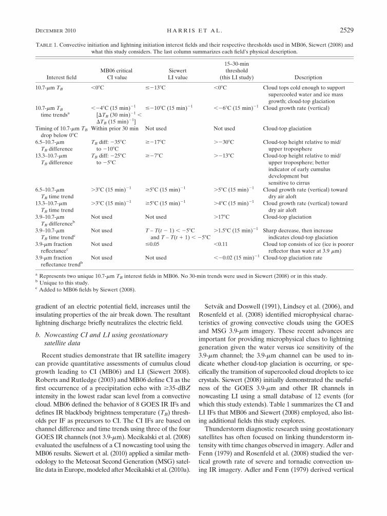
TABLE 1. Convective initiation and lightning initiation interest fields and their respective thresholds used in MB06, Siewert (2008) and
what this study considers. The last column summarizes each field’s physical description.
Interest field
MB06 critical
CI value
Siewert
LI value
15–30-min
threshold
(this LI study) Description
10.7-mm TB ,08C #2138C ,08C Cloud tops cold enough to support
supercooled water and ice mass
growth; cloud-top glaciation
10.7-mm TB
time trendsa,248C (15 min)21
[DTB (30 min)21 ,
DTB (15 min)21]
#2108C (15 min)21 ,268C (15 min)21 Cloud growth rate (vertical)
Timing of 10.7-mm TB
drop below 08C
Within prior 30 min Not used Not used Cloud-top glaciation
6.5–10.7-mm
TB difference
TB diff: 2358C
to 2108C
$2178C .2308C Cloud-top height relative to mid/
upper troposphere
13.3–10.7-mm
TB difference
TB diff: 2258C
to 258C
$278C .2138C Cloud-top height relative to mid/
upper troposphere; better
indicator of early cumulus
development but
sensitive to cirrus
6.5–10.7-mm
TB time trend
.38C (15 min)21 $58C (15 min)21 .58C (15 min)21 Cloud growth rate (vertical) toward
dry air aloft
13.3–10.7-mm
TB time trend
.38C (15 min)21 $58C (15 min)21 .48C (15 min)21 Cloud growth rate (vertical) toward
dry air aloft
3.9–10.7-mm
TB differencebNot used Not used .178C Cloud-top glaciation
3.9–10.7-mm
TB time trendcNot used T – T(t 2 1) , 258C
and T – T(t 1 1) , 258C
.1.58C (15 min)21 Sharp decrease, then increase
indicates cloud-top glaciation
3.9-mm fraction
reflectancecNot used #0.05 ,0.11 Cloud top consists of ice (ice is poorer
reflector than water at 3.9 mm)
3.9-mm fraction
reflectance trendbNot used Not used ,20.02 (15 min)21 Cloud-top glaciation rate
a Represents two unique 10.7-mm TB interest fields in MB06. No 30-min trends were used in Siewert (2008) or in this study.b Unique to this study.c Added to MB06 fields by Siewert (2008).
DECEMBER 2010 H A R R I S E T A L . 2529
velocity and divergence fields associated with active storms,
while Adler and Mack (1986) examined Cb anvil charac-
teristics and flows. Rosenfeld et al. (2008) correlated hail
and tornadoes in thunderstorms to diagnose effective
cloud-top particle radius fields, relying on the 3.9-mm
channel. Goodman et al. (1988) and Roohr and Vonder
Haar (1994) utilized geostationary imagery and light-
ning data to demonstrate general convective patterns.
With lightning detection being a burgeoning field in
remote sensing, storms that have already initiated light-
ning are central to such research. Focus has shifted from
solely CG lightning studies to total cloud lightning (TCL)
examination (i.e., combined CG and IC lightning) in the
past decade. Goodman et al. (2005) and MacGorman
et al. (2008) used TCL to infer storm severity. Addition-
ally, McCaul et al. (2009) showed how TCL can help
nudge mesoscale model resolution of microphysical pro-
cesses related to lightning.
This study is guided by the following hypotheses: 1) LI
nowcasting from GOES is a viable capability, which can
be improved with a better understanding of how to use
and interpret quantified GOES data; and 2) the 3.9-mm
channel is underutilized in LI nowcasting and can pro-
vide information on cloud-top glaciation with significant
forecast value. Overall, the primary goal of this work is
to identify which field or combination of fields provides
the most accurate and timely (predictive) indication of
imminent lightning production in convective storms.
3. Data
Five channels on the GOES-12 imager retrieve radi-
ance reflected or emitted by Earth in various wavelength
bands. The VIS channel senses reflected radiance centered
on 0.65 mm. Channels 2, 3, 4, and 6 retrieve terrestrially
emitted radiance. The 3.9-mm channel is unique in that it
senses reflected solar radiance, as well as emitted IR energy,
or emittance. The 3.9-mm channel encounters very little
attenuation or absorption by atmospheric gases or aero-
sols and is highly sensitive to water versus ice hydrome-
teors. The 6.5-mm channel is sensitive to water vapor, the
10.7-mm channel is known as the ‘‘clean window’’ since it
experiences very little atmospheric attenuation, and the
GOES-12 13.3-mm channel includes emission from car-
bon dioxide. All IR channels are 4-km resolution except
the 13.3-mm channel, which is 8-km resolution (Menzel
and Purdom 1994).
Remotely sensing TCL began as the first Lightning
Detection and Ranging (LDAR) system was installed at
Kennedy Space Center (KSC), Florida, in the 1970s. Since
then, the Lightning Mapping Array (LMA) was born out
of lightning research at New Mexico Tech (Krehbiel et al.
2000; Thomas et al. 2001). The LMA locates lightning
radiation sources in three spatial dimensions and time. The
array is a mesoscale network of Global Positioning System
Time-of-Arrival (GPS-TOA) sensors that detect very high
frequency (VHF) signals at unused television frequencies.
The arrays are ;(60 3 80) km in size. For this study, we
used the four-dimensional (4D) TCL data from three of
the four existing LMAs. The Central Oklahoma LMA
(OKLMA) and the North Alabama LMA (NALMA)
consist of 11 and 13 GPS VHF receivers, respectively,
which sense lightning source radiation in the 54–88-MHz
range. The Washington, D.C., LMA (DCLMA) is the
newest operational LMA, and it contains 10 sensors that
detect lightning sources in the 192–198-MHz radio fre-
quency range. The higher VHF channel is used in the
DCLMA to limit the effects of increased radio frequency
noise in an urban environment (Krehbiel et al. 2006). The
LMA’s flash detection efficiency approaches 100% within
the 60 3 80-km array and decreases outward. The location
accuracy degrades quadratically with distance from the
center (Koshak et al. 2004; Thomas et al. 2004). The
NALMA, as noted by Goodman et al. (2005), is nominally
accurate to within 50 m inside the 150-km array center.
This study used preprocessed ‘‘decimated’’ LMA data.
While decimated data are not as detailed as fully post-
processed data, they are sufficiently detailed for most uses
(Rison et al. 2003). From these data, the following in-
formation was used for each source detected by the array:
decimal time, latitude, longitude, and altitude.
The 4D Lightning Surveillance System (4DLSS), which
replaced the legacy LDAR system, has both a CG and
TCL sensor array. Like the LMA, the 4DLSS’s TCL array
uses VHF and TOA techniques to pinpoint lightning
sources. The array consists of nine 60–66-MHz VHF
sensors spread across an estimated 45 3 65 km2 area that
includes the KSC complex. The flash detection efficiency
is 100% within the array and 90% at 111 km from the
array center. Like the LMA, the location accuracy de-
grades quadratically with distance from the center. The
location error is ,2 km at 111 km from the center
(Murphy et al. 2008). The 4DLSS is slightly less accurate
than the LMA at distances beyond its 45 3 65 km2 net-
work since the 4DLSS array area is smaller. 4DLSS data
were obtained from the National Aeronautics and Space
Administration (NASA) (NASA 2010). The Cloud-to-
Ground Lightning Surveillance System that is part of the
4DLSS was not used in this study.
4. Processing methodology
As a means of meeting this study’s objectives and
addressing the research hypotheses, the following anal-
ysis procedures are developed. This study considers
summertime convection that occurred between 24 May
2530 J O U R N A L O F A P P L I E D M E T E O R O L O G Y A N D C L I M A T O L O G Y VOLUME 49
and 23 August 2009, and therefore we expect the results
will be most applicable during this time of year.
a. Study region considerations
Before building a storm catalog, the accuracy of each
4D lightning platform is considered to narrow the focus
areas. Similar to Goodman et al. (2005), potential storm
cases were limited to within 150 km of each LMA array
center. Specific LMA detection efficiencies were not
available to compare with the 4DLSS; however, since the
4DLSS has a smaller array area, its effective range is
smaller. Therefore, the 90% detection efficiency radius
(i.e., 100 km) was arbitrarily chosen to restrict the Florida
cases in this study, yet a few exceptions were allowed for
ideal LI events. Figures 1a–d show the regions of interest.
b. Identifying potential lightning initiators
After the usable radii for each 4D lightning region were
determined, GOES-12 VIS imagery was examined each
day for potential LI events by subjectively searching
for cumulus fields that later developed into convective
storms. Key to the search was newly initiated convection
occurring between 1230 and 2359 UTC.1 Storms with
nearby preexisting convection (i.e., within 10 km) were
generally excluded from this study because of possible
‘‘contamination’’ from overlying cirrus clouds. Even thin
cirrus above developing cumulus clouds will result in
colder cloud top TB values than actually exist, while also
altering the microphysical properties estimated from the
3.9-mm channel. Potential storm days for each region
were catalogued based on the criteria in Table 2, provided
the availability of satellite and lightning data. Once cat-
aloging was complete, GOES-12 data were collected for
all ‘‘Excellent’’ cases. Some ‘‘Good’’ and a few ‘‘Fair’’
cases were used as well, after closer examination revealed
less contamination than initially assessed.
c. LMA data
The 4D TCL datasets are extremely voluminous. A
single storm can have O(104–105) individual lightning
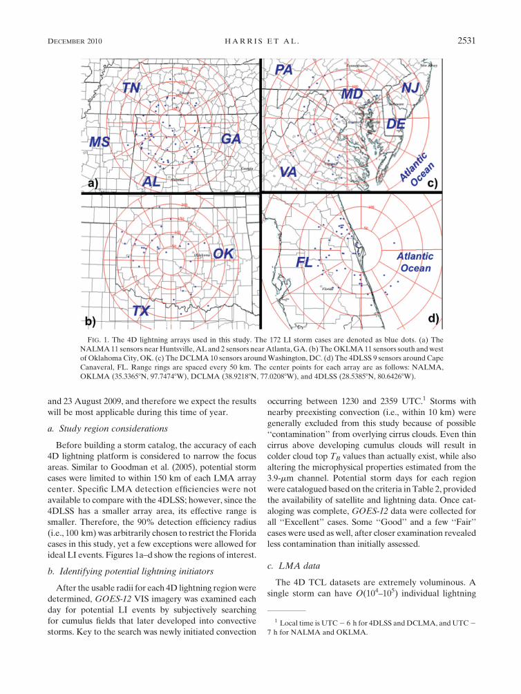
FIG. 1. The 4D lightning arrays used in this study. The 172 LI storm cases are denoted as blue dots. (a) The
NALMA 11 sensors near Huntsville, AL and 2 sensors near Atlanta, GA. (b) The OKLMA 11 sensors south and west
of Oklahoma City, OK. (c) The DCLMA 10 sensors around Washington, DC. (d) The 4DLSS 9 sensors around Cape
Canaveral, FL. Range rings are spaced every 50 km. The center points for each array are as follows: NALMA,
OKLMA (35.33658N, 97.74748W), DCLMA (38.92188N, 77.02088W), and 4DLSS (28.53858N, 80.64268W).
1 Local time is UTC 2 6 h for 4DLSS and DCLMA, and UTC 2
7 h for NALMA and OKLMA.
DECEMBER 2010 H A R R I S E T A L . 2531
radiation source events, and single flashes can contain
anywhere from a few to .1000 sources. Many of the po-
tential storm days had $1 million source events. Thou-
sands of source events can occur in only 1–2 s. Recall, the
goal was to identify when LI occurred (i.e., the first source
in a Cb). To reduce data volume while ensuring event
(flash) detection, the 4D data were processed using two
flash-grouping algorithms, similar to the National Light-
ning Detection Network (NLDN; Orville 1991; Orville
and Huffines 2001) flash-grouping algorithm. One algo-
rithm processed 4D lightning data for the three LMAs,
and the second algorithm grouped lightning sources into
probable flashes for the 4DLSS. Also tracked were first-
time CG occurrences using NLDN data in order to verify
the 4D flash-grouping results, and additionally to measure
the time lag from first-time IC to CG lightning.
The LMA flash-grouping algorithm for this research was
supplied by the National Space Science Technology Center
at the University of Alabama in Huntsville (McCaul et al.
2009). The algorithm employs time and space proximity
criteria to identify the sources belonging to a given flash.
Sources are assumed to belong to the same flash if they
occur less than 0.3 s apart in time and also satisfy a spatial
separation requirement.
Sources were assigned a flash number, followed by the
filtering of what McCaul et al. (2009) termed ‘‘singletons.’’
A flash containing only one source is considered to be
either erroneous or atmospheric VHF noise. Therefore,
flashes with 2–101 sources define an accurate flash mea-
surement. This study assumes that a flash contains at least
4 sources. After filtering, the first source within the flash is
defined to be the originating source. Subsequently, flash-
grouped LMA files were created for each potential storm
day containing flash time and location (latitude, longitude,
and altitude) represented by the parent source of each
flash.
d. 4DLSS data
Because of 4DLSS data format differences, a different
flash-grouping algorithm was needed. McNamara (2002)
and Nelson (2002) used a flash-grouping algorithm to
cluster lightning sources for the original LDAR sensor.
This study used the flash-grouping algorithm from Nelson
and the new 4DLSS accuracy numbers identified by
Murphy et al. (2008) to cluster lightning sources into
probable flashes. Finally, for consistency, the 4DLSS clus-
tering thresholds were changed to more closely match those
used in the LMA algorithm. Table 3 shows the original
LDAR flash-grouping algorithm’s clustering thresholds
alongside the new 4DLSS flash-grouping algorithm, as
well as the LMA thresholds for comparison.
As with the LMA data, a valid flash contained at least
4 sources; all flashes with ,4 sources were removed.
Latitude–longitude–altitude coordinates and the geodetic
approximation calculations that take Earth’s curvature
into consideration were used (McNish 2010). Subse-
quently, flash-grouped 4DLSS files were created for
each storm day, also listing each flash by time and lo-
cation represented by the parent source of each flash.
e. Identifying individual storm cases
Once the lightning and satellite data were prepared,
individual storm cases were identified. For each day with
active lightning, individual cells were studied from the pre-
cumulus stage to LI. (Convective cells that failed to pro-
duce lightning were generally ignored for this study.) The
sample storm set was limited to a specific time window each
day as the 3.9-mm reflectance (ref39) becomes undefined as
the solar zenith angle approaches 908 (i.e., sun on horizon).
Specifically, Lindsey et al. (2006) determined the GOES
ref39 to be most usable when the solar zenith angle is #688.
Individual storm cases were selected within the following
approximate time windows based on Lindsey et al. (2006)’s
688 rule: NALMA (1305–2230 UTC), 4DLSS (1242–
2208 UTC), OKLMA (1351–2315 UTC), and DCLMA
(1230–2152 UTC). Both the 1-min grouped NLDN CG
and 4D IC data were overlaid on top of the satellite im-
ages. The NLDN observes a small percentage of IC flashes
while the 4D lightning array can observe CG flashes.
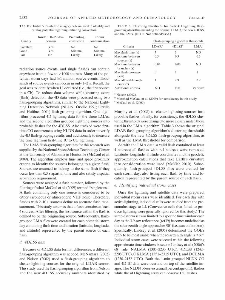
TABLE 2. Initial VIS satellite imagery criteria used to identify and
catalog potential lightning-initiating convection.
Quality
Inside 100–150-km
domain
Preexisting
convection
Cirrus
contamination
Excellent Yes No No
Good Yes Minimal Minimal
Fair No Likely Likely
TABLE 3. Clustering thresholds for each 4D lightning flash-
grouping algorithm including the original LDAR, the new 4DLSS,
and the LMA. (ND 5 Not defined/used.)
Criteria
Flash-grouping algorithm thresholds
LDARa 4DLSSb LMAc
Max flash time (s) 3 3 ND
Max time between
sources (s)
0.5 0.3 0.3
Max time between
branches (s)
0.03 0.03 ND
Max flash coverage
(km)
5 1 1
Max allowable angle
error (8)
1 2.9 2.9
Additional criteria ND ND Variousc
a Nelson (2002).b Matched McCaul et al. (2009) for consistency in this study.c McCaul et al. (2009).
2532 J O U R N A L O F A P P L I E D M E T E O R O L O G Y A N D C L I M A T O L O G Y VOLUME 49
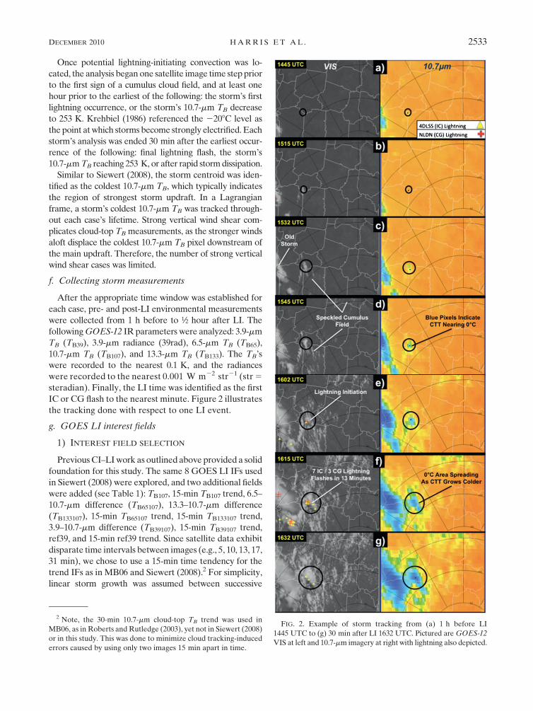
Once potential lightning-initiating convection was lo-
cated, the analysis began one satellite image time step prior
to the first sign of a cumulus cloud field, and at least one
hour prior to the earliest of the following: the storm’s first
lightning occurrence, or the storm’s 10.7-mm TB decrease
to 253 K. Krehbiel (1986) referenced the 2208C level as
the point at which storms become strongly electrified. Each
storm’s analysis was ended 30 min after the earliest occur-
rence of the following: final lightning flash, the storm’s
10.7-mm TB reaching 253 K, or after rapid storm dissipation.
Similar to Siewert (2008), the storm centroid was iden-
tified as the coldest 10.7-mm TB, which typically indicates
the region of strongest storm updraft. In a Lagrangian
frame, a storm’s coldest 10.7-mm TB was tracked through-
out each case’s lifetime. Strong vertical wind shear com-
plicates cloud-top TB measurements, as the stronger winds
aloft displace the coldest 10.7-mm TB pixel downstream of
the main updraft. Therefore, the number of strong vertical
wind shear cases was limited.
f. Collecting storm measurements
After the appropriate time window was established for
each case, pre- and post-LI environmental measurements
were collected from 1 h before to ½ hour after LI. The
following GOES-12 IR parameters were analyzed: 3.9-mm
TB (TB39), 3.9-mm radiance (39rad), 6.5-mm TB (TB65),
10.7-mm TB (TB107), and 13.3-mm TB (TB133). The TB’s
were recorded to the nearest 0.1 K, and the radiances
were recorded to the nearest 0.001 W m22 str21 (str 5
steradian). Finally, the LI time was identified as the first
IC or CG flash to the nearest minute. Figure 2 illustrates
the tracking done with respect to one LI event.
g. GOES LI interest fields
1) INTEREST FIELD SELECTION
Previous CI–LI work as outlined above provided a solid
foundation for this study. The same 8 GOES LI IFs used
in Siewert (2008) were explored, and two additional fields
were added (see Table 1): TB107, 15-min TB107 trend, 6.5–
10.7-mm difference (TB65107), 13.3–10.7-mm difference
(TB133107), 15-min TB65107 trend, 15-min TB133107 trend,
3.9–10.7-mm difference (TB39107), 15-min TB39107 trend,
ref39, and 15-min ref39 trend. Since satellite data exhibit
disparate time intervals between images (e.g., 5, 10, 13, 17,
31 min), we chose to use a 15-min time tendency for the
trend IFs as in MB06 and Siewert (2008).2 For simplicity,
linear storm growth was assumed between successive
FIG. 2. Example of storm tracking from (a) 1 h before LI
1445 UTC to (g) 30 min after LI 1632 UTC. Pictured are GOES-12
VIS at left and 10.7-mm imagery at right with lightning also depicted.
2 Note, the 30-min 10.7-mm cloud-top TB trend was used in
MB06, as in Roberts and Rutledge (2003), yet not in Siewert (2008)
or in this study. This was done to minimize cloud tracking-induced
errors caused by using only two images 15 min apart in time.
DECEMBER 2010 H A R R I S E T A L . 2533
satellite images (even though deep convection often ex-
hibits highly nonlinear atmospheric tendencies). The 3.9-,
6.5-, and 13.3-mm channels were not included as stand-
alone IFs, as other studies relating these fields to cloud
properties determined that the aforementioned channels
show little to no significant ‘‘stand alone’’ signal leading up
to LI (MB06; Siewert 2008).
2) 3.9-mm REFLECTANCE
Previous research demonstrated the ref39’s usefulness,
particularly with regard to water-versus-ice delineation in
convective clouds (Setvak and Doswell 1991; Lindsey
et al. 2006). The total 3.9-mm radiance received at the
satellite, R3.9mm, is described as
R3.9mm
5 ref39 1 e3.9mm
Remit39mm
(T), (1)
where the second term is the product of an object’s
3.9-mm emittance and its emissivity, e3.9mm. The sensed
objects (cloud mass) are assumed to be perfect black-
bodies at 3.9 mm, and thus e3.9mm 1 ref39 5 1, for clouds of
sufficient optical thickness. Obtaining ref39 from Eq. (1)
follows the methodology of Setvak and Doswell (1991)
and Lindsey et al. (2006).
The total amount of Earth-absorbed solar radiance at
3.9 mm, assuming the Sun’s blackbody temperature is
5800 K and using the GOES-12 Planck function con-
stants and solar radiance equation, is given by
Remit3.9mm
(Tsun
) 5fk1
3.9mm
expfk2
3.9mm
bc13.9mm
1 (bc23.9mm
Tsun
)
" #� 1
,
(2)
where fk1, fk2, bc1, and bc2 are all 3.9-mm GOES-specific
constants (CIMSS/SSEC 2010). Next, the 3.9-mm solar
flux at the top of the atmosphere is given by
S3.9mm
(r, j) 5 [Remit3.9mm
(Tsun
)](Rsun
/rE
)2 cosj, (3)
where Rsun is the sun’s radius (6.96 3 108 km), rE is
Earth’s orbit radius (1.496 3 1011 km), and cosj uses the
solar zenith angle (j).
With the solar flux calculated, the 3.9-mm emitted
Planck blackbody radiance is estimated, as noted from
Kidder and Vonder Haar (1995), by
B3.9mm
(TB107
) 5c
1l�5
expc
2
lTB107
� �� 1
, (4)
where c1 5 1.19104 3 10216 W m2 (str)21, c2 5
0.014 387 69 m K, and l 5 3.9 3 1026 mm [multiplied by
1026 to obtain the emitted Planck radiance in terms of
W m2 (sr)21 mm21]. Here, the Planck curve is based on
our TB107 measurement. The corresponding 3.9-mm point
on the Planck curve is the 3.9-mm emittance, assuming the
TB107 measurement emanated from a perfect blackbody.
For optically thick clouds like a deep cumulus, this is a
safe assumption (Lindsey et al. 2006). Finally, ref39 is
calculated using
ref39 5R
3.9mm� B
3.9mm(T
B107)
S3.9mm
(r, j)� B3.9mm
(TB107
). (5)
Some minimal error is introduced in assuming only
isotropically scattering spherical cloud and precipitation
particles (Setvak and Doswell 1991).
3) LIGHTNING INITIATION DATABASE
A database was prepared for temporal and regional
comparison analysis, involving the following procedures.
First, all storms were oriented to the same temporal plane
by converting times to decimal hour. The initial time,
whether 1402 or 2231 UTC, for example, is set to 0 min.
This standardization allowed for easier comparative storm
analysis. Second, the hour period prior to LI is subdivided
into 15-min intervals to help estimate the predictive capa-
bility of each IF. Quarter-hour intervals were chosen as
GOES data are currently available every 15 min on av-
erage. In addition, most of the cases developed from the
pre-cumulus stage to LI in #1 h. The database consisted of
IF data at 60 min (LI–60), 45 min (LI–45), 30 min (LI–30)
and 15 min before LI (LI–15), and at the LI time (LI–0).
As satellite image intervals and LI-related times
consistently did not match in the hour prior to LI, linear
interpolation was performed on each IF between satel-
lite data points. Some introduced interpolation error
may occur where some IFs exhibit more nonlinear ten-
dencies than others, but is expected to be minor (,5%).
5. Results
Following the methodology above, 172 total LI cases
over four geographical regions were analyzed (Fig. 1); at
least 30 cases were collected for each region, while two
exceptions were made. First, because of a lack of data, five
NALMA cases are only partially complete with respect to
time. For NALMA LI–60, there are 53/58 cases (i.e., five
less than the total), and for LI–45 there are 57/58 cases
(i.e., one less than the total). Insignificant degradation to
our results is expected given the relatively large sample
size. Secondly, 22/172 cases (i.e., 12.8%) occurred outside
the 100–150-km array areas. The aforementioned excep-
tion was made only if the 4D data appeared to observe the
individual storm case well, as defined when a CG flash
2534 J O U R N A L O F A P P L I E D M E T E O R O L O G Y A N D C L I M A T O L O G Y VOLUME 49
occurred within 4.6–6.9 min of an IC flash, depending on
the region. The average time between IC and CG flashes in
this study—6.9 min for NALMA, 6.8 min for 4DLSS,
4.6 min for DCLMA, and 4.7 min for OKLMA—matched
very closely with the approximate 5–10-min interval noted
by Williams and Orville (1989) and Williams et al. (2005).
Any lightning timing error caused by this exception is
determined to be ,(2–3) min. Of interest, some storms in
three of the regions—13.8% NALMA, 9.8% 4DLSS, and
25.8% OKLMA—exhibited 0 CG flashes within 30 min
after the first IC flash.3
a. Behavior of individual GOES interest fields
As a means of limiting the presentation, Figs. 3a–g
depict the IF results for one LI event in the 4DLSS re-
gion (case 39). All 172 cases do not follow the exact
behavior of this LI event; however, the qualitative de-
scriptions represent the entire dataset very well.
Figure 3a shows all four GOES IR channels’ behavior in
the hour before LI. As expected, a gradual TB107 decrease
is seen between LI–60 and LI–45, with a more precipitous
TB107 drop especially after LI–30 as the convective cloud
grows rapidly into a colder environment. The precipitous
TB107 drop for some cases, particularly in the 4DLSS re-
gion, did not occur until LI–15. Very few cases exhibited
only gradual TB decreases in the 15 min prior to LI, indi-
cating that our dataset contains primarily rapidly devel-
oping storms (i.e., reach LI in ,1 h; versus slow-building
lightning initiators). Also, OKLMA storms showed the
most precipitous TB107 decreases of all regions, and the
drops also occur earlier in the storm’s development. One
possible reason may be that the OKLMA region possessed
higher overall instability compared to the other locations,
although we cannot substantiate this claim at this time.
The 15-min TB107 trend (Fig. 3b) appears weakly nega-
tive (0 to 26 K) for most cases until about LI–30. The
trend decreases significantly (.6 K) from LI–15 to LI–
30 min as the updraft increases. The OKLMA TB107 trends
maintain a relatively strong decrease (.6 K) from early in
the storm’s development leading up to LI, unlike in the
other regions, possibly because of more rapidly developing
storms (as noted above). Decreases in TB107 of .10 K at
LI–0 are common for all regions. Compared to other IFs,
the TB107 trend exhibited moderate variability between
cases.
The TB65107 and TB133107 IFs (Fig. 3c) display similar
characteristics. Each of the IFs begins low: TB65107 is lower
than the TB133107 because of the TB65 field having a much
colder TB with respect to the TB107 field. Both IFs show
steady increases (i.e., becoming less negative) in all four
regions, as the convective clouds approach LI. Some TB65107
and TB133107 values occasionally became neutral near LI–30
before continuing to increase shortly thereafter. Although
4DLSS case 39 does not exhibit this neutral behavior, one
potential cause for this temporarily steady behavior may be
linked to the convective cloud reaching a capped or stable
atmospheric layer and briefly slowing the storm’s growth.
The TB65107 and TB133107 difference IFs display very little
variability between storms when compared to the other IFs.
Figure 3d shows the TB65107 and TB133107 15-min time
trend IFs. A weak positive tendency in both IFs occurs
during the early storm development stage (,4 K). By LI–
30, most storms exhibit a sharper positive trend. The sep-
aration between the two IFs occurs as the TB65107 trend is
larger than the TB133107 trend (.4–6 K, versus 3–5 K)
after LI–45. As the TB107 decreases rapidly after LI–30, the
gap between it and TB65 decreases more quickly than the
TB107 and TB133 curves (Fig. 3a). Like the TB65107 and
TB133107 IFs, their respective trends show little variability
between storms when compared to the other IFs.
The TB39107 difference IF (Fig. 3e) typically had a
steady or perhaps a slight increase in the early storm de-
velopment stage. The increase is often followed by a
sharp decrease, then a further increase about 15–30 min
prior to LI, as exhibited by the TB39107 curve. The sharp
increase was not as apparent for DCLMA, and typically
did not occur until the last 15 min before LI. Similarly, the
4DLSS cases showed this increase most often from LI–15
to LI–0. Siewert (2008) suggested the sharp TB39107 in-
crease that follows a slight dip or steadiness indicates a
rapid increase in ice flux within the storm. Higher ice
content decreases the TB39’s reflective component more
rapidly than the emitted component, as approximated by
TB107. The TB39107 difference exhibits the largest vari-
ability between storms compared to the other IFs.
The ref39 IF (Fig. 3e) shows little variability between
storms when compared with the other IFs. A steady to
sharp ref39 decrease is often noticed in the hour before
LI. The sharpest drops generally occurred 15–45 min
prior to LI. The ref39 occasionally mirrored the slight
increase–decreasing trend that the TB39107 difference IF
exhibits, particularly in the 4DLSS region. Furthermore,
nearly all of the 172 storms had ref39 values #0.05 (5%)
from LI–15 to LI–0. Setvak and Doswell (1991) suggest that
a Cb has reached complete glaciation at this fraction re-
flectance threshold. A glaciated cloud infers greater light-
ning potential since charge separation occurs rapidly with
ice crystal and supercooled droplet collisions (Reynolds
et al. 1957).
The TB39107 and ref39 15-min time trends exhibit
characteristics similar to those discussed above. Note the
3 Regional comparisons among the four datasets from the light-
ning mapping systems will be presented and discussed in a com-
panion paper.
DECEMBER 2010 H A R R I S E T A L . 2535
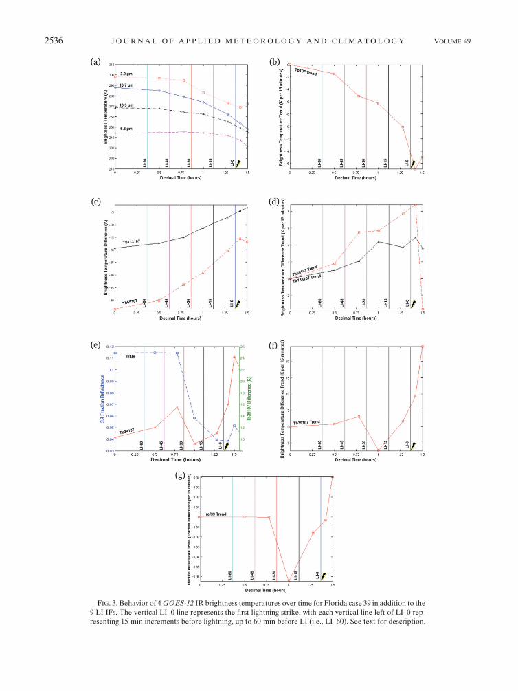
FIG. 3. Behavior of 4 GOES-12 IR brightness temperatures over time for Florida case 39 in addition to the
9 LI IFs. The vertical LI–0 line represents the first lightning strike, with each vertical line left of LI–0 rep-
resenting 15-min increments before lightning, up to 60 min before LI (i.e., LI–60). See text for description.
2536 J O U R N A L O F A P P L I E D M E T E O R O L O G Y A N D C L I M A T O L O G Y VOLUME 49
weakly positive TB39107 trend in Fig. 3f between LI–60 and
LI–45, followed by a quick decrease then strong increase
by LI–15. Much less TB39107 trend variability is seen be-
tween storms when compared to TB39107. The 15-min ref39
trend (Fig. 3g) also shows small variability between storms
when compared to the other IFs. The ref39 trend generally
remains negative throughout the hour leading up to LI
and has the most pronounced negative trend 15–45 min
before LI.
b. Interest field variability
After each of the 172 cases was qualitatively analyzed,
statistics for each of the five LI datasets, from LI–60 to
LI–0, were compiled. This was done to show the vari-
ability in IFs as a function of time leading up to LI.
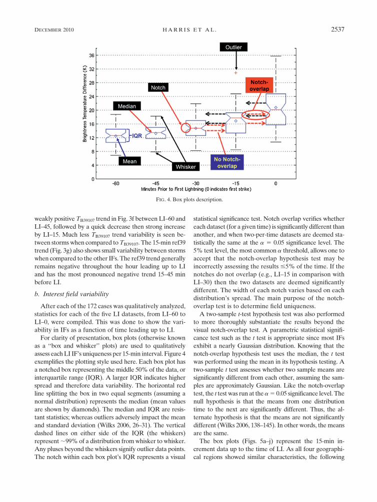
For clarity of presentation, box plots (otherwise known
as a ‘‘box and whisker’’ plots) are used to qualitatively
assess each LI IF’s uniqueness per 15-min interval. Figure 4
exemplifies the plotting style used here. Each box plot has
a notched box representing the middle 50% of the data, or
interquartile range (IQR). A larger IQR indicates higher
spread and therefore data variability. The horizontal red
line splitting the box in two equal segments (assuming a
normal distribution) represents the median (mean values
are shown by diamonds). The median and IQR are resis-
tant statistics; whereas outliers adversely impact the mean
and standard deviation (Wilks 2006, 26–31). The vertical
dashed lines on either side of the IQR (the whiskers)
represent ;99% of a distribution from whisker to whisker.
Any pluses beyond the whiskers signify outlier data points.
The notch within each box plot’s IQR represents a visual
statistical significance test. Notch overlap verifies whether
each dataset (for a given time) is significantly different than
another, and when two-per-time datasets are deemed sta-
tistically the same at the a 5 0.05 significance level. The
5% test level, the most common a threshold, allows one to
accept that the notch-overlap hypothesis test may be
incorrectly assessing the results #5% of the time. If the
notches do not overlap (e.g., LI–15 in comparison with
LI–30) then the two datasets are deemed significantly
different. The width of each notch varies based on each
distribution’s spread. The main purpose of the notch-
overlap test is to determine field uniqueness.
A two-sample t-test hypothesis test was also performed
to more thoroughly substantiate the results beyond the
visual notch-overlap test. A parametric statistical signifi-
cance test such as the t test is appropriate since most IFs
exhibit a nearly Gaussian distribution. Knowing that the
notch-overlap hypothesis test uses the median, the t test
was performed using the mean in its hypothesis testing. A
two-sample t test assesses whether two sample means are
significantly different from each other, assuming the sam-
ples are approximately Gaussian. Like the notch-overlap
test, the t test was run at the a 5 0.05 significance level. The
null hypothesis is that the means from one distribution
time to the next are significantly different. Thus, the al-
ternate hypothesis is that the means are not significantly
different (Wilks 2006, 138–145). In other words, the means
are the same.
The box plots (Figs. 5a–j) represent the 15-min in-
crement data up to the time of LI. As all four geographi-
cal regions showed similar characteristics, the following
FIG. 4. Box plots description.
DECEMBER 2010 H A R R I S E T A L . 2537
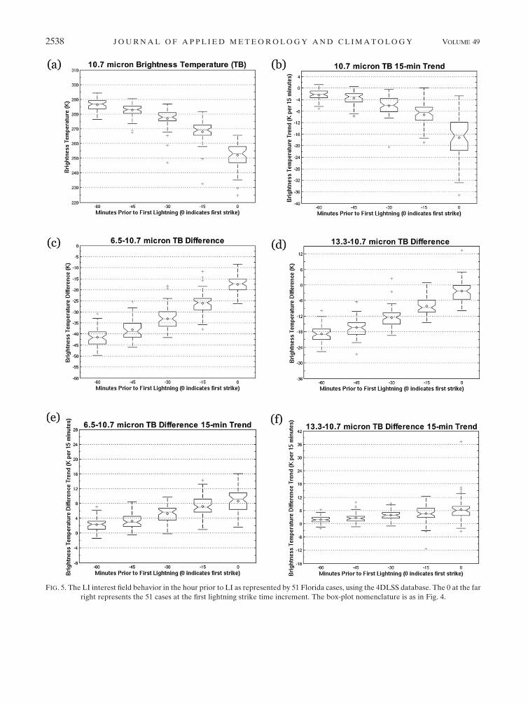
FIG. 5. The LI interest field behavior in the hour prior to LI as represented by 51 Florida cases, using the 4DLSS database. The 0 at the far
right represents the 51 cases at the first lightning strike time increment. The box-plot nomenclature is as in Fig. 4.
2538 J O U R N A L O F A P P L I E D M E T E O R O L O G Y A N D C L I M A T O L O G Y VOLUME 49
qualitative assessment based on the 4DLSS box plots ap-
plies to all regions unless otherwise noted. A few t-test re-
sults vary from the notch-overlap test since the t test is
testing against a distribution and its mean, while the notch-
overlap tests against a distribution and its median. Final
determination was based on the t-test results. Although the
t-test findings are not shown explicitly, we regularly invoke
the results during each IF’s notch-overlap discussion.
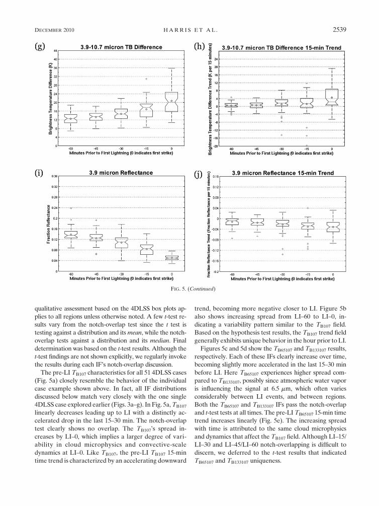
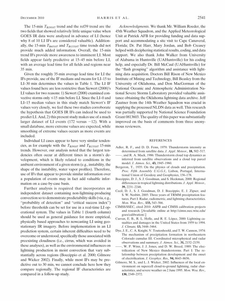
The pre-LI TB107 characteristics for all 51 4DLSS cases
(Fig. 5a) closely resemble the behavior of the individual
case example shown above. In fact, all IF distributions
discussed below match very closely with the one single
4DLSS case explored earlier (Figs. 3a–g). In Fig. 5a, TB107
linearly decreases leading up to LI with a distinctly ac-
celerated drop in the last 15–30 min. The notch-overlap
test clearly shows no overlap. The TB107’s spread in-
creases by LI–0, which implies a larger degree of vari-
ability in cloud microphysics and convective-scale
dynamics at LI–0. Like TB107, the pre-LI TB107 15-min
time trend is characterized by an accelerating downward
trend, becoming more negative closer to LI. Figure 5b
also shows increasing spread from LI–60 to LI–0, in-
dicating a variability pattern similar to the TB107 field.
Based on the hypothesis test results, the TB107 trend field
generally exhibits unique behavior in the hour prior to LI.
Figures 5c and 5d show the TB65107 and TB133107 results,
respectively. Each of these IFs clearly increase over time,
becoming slightly more accelerated in the last 15–30 min
before LI. Here TB65107 experiences higher spread com-
pared to TB133107, possibly since atmospheric water vapor
is influencing the signal at 6.5 mm, which often varies
considerably between LI events, and between regions.
Both the TB65107 and TB133107 IFs pass the notch-overlap
and t-test tests at all times. The pre-LI TB65107 15-min time
trend increases linearly (Fig. 5e). The increasing spread
with time is attributed to the same cloud microphysics
and dynamics that affect the TB107 field. Although LI–15/
LI–30 and LI–45/LI–60 notch-overlapping is difficult to
discern, we deferred to the t-test results that indicated
TB65107 and TB133107 uniqueness.
FIG. 5. (Continued)
DECEMBER 2010 H A R R I S E T A L . 2539
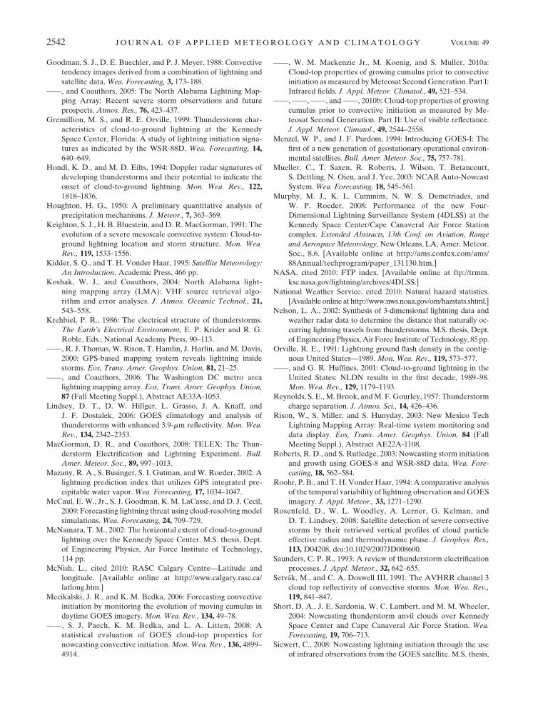
The TB133107 15-min time trend’s increase is even subtler
than the TB65107 trend. Figure 5f also indicates much less
spread than the TB65107 trend for the same reason dis-
cussed above. Less spread reduces potential notch overlap
and therefore increases possible uniqueness likelihood;
however, Fig. 5f indicates considerable notch overlap, and
hence little unique value, because of the subtlety of the
TB133107 trend’s increase. The TB133107 trend exhibits rel-
atively redundant information at longer lead times; how-
ever, in three of the four regions (i.e., NALMA, OKLMA,
and DCLMA) some useful trend information is found at
LI–15.
In Fig. 5g, TB39107 increases linearly at first and then
accelerates 15–30 min before LI. Any notch overlap be-
tween LI–0 and LI–15 for 4DLSS is subtle. The accentu-
ated TB39107 increase between LI–15 and LI–30 matches
the average LI lead time over which TB39107 may provide
useful information. The TB39107 15-min time trend increases
slightly leading up to LI, while the distribution’s spread
widens (Fig. 5h). The individual trend seen for case 39 is
apparent, although is much less for the 4DLSS domain
compared to the other regions. The characteristic increase–
decrease–increase signal documented by Siewert (2008) is
somewhat apparent in the TB39107 15-min time trend dis-
tributions; however, this cannot be statistically validated
because of marginal notch-overlap and t-test results. Al-
though the up–down–up tendency was noted in individual
cases, this tendency is likely washed out when considered
within a larger dataset, since this TB39107 trend behavior
often occurs at different times for each storm from LI–15 to
LI–45 min. In addition, the TB39107 trend shows little unique
information more than 15 min before LI.
As ice content increases volumetrically within a grow-
ing storm, ref39 decreases as depicted in Fig. 5i. The
decrease is primarily linear and perhaps very slightly ac-
celerated in the last 15–30 min for each region. Regions
NALMA, 4DLSS, and DCLMA show complete cloud-
top glaciation (i.e., ref39 , 0.05) by LI–0, while over
OKLMA, a 0.07 (7%) 3.9-mm fraction reflectance is the
average; this small difference is speculated to be a satel-
lite view-angle affect, especially since the OKLMA is
farthest west (see Lindsey et al. 2006)4. The ref39’s notch-
overlap and t-test results indicate significant unique in-
formation at least 45 min ahead of LI. Although a general
decreasing tendency is noted in the ref39 15 min trend
(Fig. 5j), the decreases are too subtle. Overall, the ref39
trend provides very little unique information before LI.
6. Conclusions
Upon the examination of 172 LI events over the four
LMA networks in GOES IR IFs, 8 out of 10 LI IFs con-
sidered have at least some unique value in identifying LI
across all regions. Statistical significance tests were per-
formed as a means of quantifying IF uniqueness. Table 1
(fourth column) summarizes the findings of Figs. 3a–g, 5a–j,
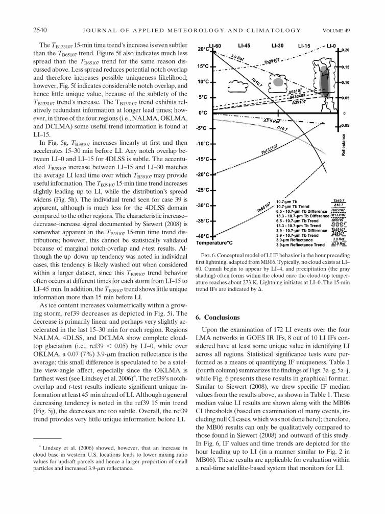
while Fig. 6 presents these results in graphical format.
Similar to Siewert (2008), we drew specific IF median
values from the results above, as shown in Table 1. These
median value LI results are shown along with the MB06
CI thresholds (based on examination of many events, in-
cluding null CI cases, which was not done here); therefore,
the MB06 results can only be qualitatively compared to
those found in Siewert (2008) and outward of this study.
In Fig. 6, IF values and time trends are depicted for the
hour leading up to LI (in a manner similar to Fig. 2 in
MB06). These results are applicable for evaluation within
a real-time satellite-based system that monitors for LI.
FIG. 6. Conceptual model of LI IF behavior in the hour preceding
first lightning, adapted from MB06. Typically, no cloud exists at LI–
60. Cumuli begin to appear by LI–4, and precipitation (the gray
shading) often forms within the cloud once the cloud-top temper-
ature reaches about 273 K. Lightning initiates at LI–0. The 15-min
trend IFs are indicated by D.
4 Lindsey et al. (2006) showed, however, that an increase in
cloud base in western U.S. locations leads to lower mixing ratio
values for updraft parcels and hence a larger proportion of small
particles and increased 3.9-mm reflectance.
2540 J O U R N A L O F A P P L I E D M E T E O R O L O G Y A N D C L I M A T O L O G Y VOLUME 49
The 15-min TB39107 trend and the ref39 trend are the
two fields that showed relatively little unique value when
GOES IR data were analyzed in advance of LI (hence
why 8 of 10 LI IFs are considered valuable). Addition-
ally, the 15-min TB65107 and TB133107 time trends did not
provide much added information. Overall, the 15-min
trend IFs provide more awareness to imminent LI. Most
fields appear fairly predictive at 15–45 min before LI,
with an average lead time for all fields and regions near
35 min.
Given the roughly 35-min average lead time for LI the
IFs provide, use of the IF medians and means for LI–15 to
LI–30 min determines the values in Table 1. The LI IF
values found here are less restrictive than Siewert (2008)’s
LI values for two reasons: 1) Siewert (2008) examined con-
vective storms only #15 min before LI. Since the LI–0 and
LI–15 median values in this study match Siewert’s IF
values very closely, we feel these two studies corroborate
the hypothesis that GOES IR IFs can indeed be used to
predict LI. And, 2) this present study makes use of a much
larger dataset of LI events (172 versus ;12). With a
small database, more extreme values are expected, while
smoothing of extreme values occurs as more events are
included.
Individual LI cases appear to have very similar tenden-
cies, as for example with the TB39107 and TB133107 15-min
trends. However, our analysis noted that the largest ten-
dencies often occur at different times in a storm’s de-
velopment, which is likely related to conditions in the
ambient environment of a given storm (e.g., instability, the
shape of the instability, water vapor profiles). Therefore,
use of IFs that appear to provide similar information over
a population of events may in fact add valuable infor-
mation on a case-by-case basis.
Further analysis is required that incorporates an
independent dataset containing non-lightning-producing
convection so to demonstrate predictability skills (via, e.g.,
‘‘probability of detection’’ and ‘‘critical success index’’)
before thresholds can be set for use in a real-time LI op-
erational system. The values in Table 1 (fourth column)
should be used as general guidance for more empirical,
physically based approaches to nowcasting LI using geo-
stationary IR imagery. Before implementation in an LI
prediction system, certain inherent difficulties need to be
overcome or understood, specifically those associated with
preexisting cloudiness (i.e., cirrus, which was avoided in
these analyses), as well as the environmental influences on
lightning production in moist convection that vary sub-
stantially across regions (Boccippio et al. 2000; Gilmore
and Wicker 2002). Finally, while most IFs may be pre-
dictive out to 30 min, we cannot conclude here how they
compare regionally. The regional IF characteristics are
compared in a follow-up study.
Acknowledgments. We thank Mr. William Roeder, the
45th Weather Squadron, and the Applied Meteorological
Unit at Patrick AFB for providing funding and data sup-
port and accommodating a site visit to Cape Canaveral,
Florida; Dr. Pat Harr, Mary Jordan, and Bob Creasey
helped with deciphering statistical results, coding, and data
support. We also thank John Walker from University
of Alabama in Huntsville (UAHuntsville) for his coding
help, and especially Dr. Bill McCaul (UAHuntsville) for
the ‘‘flash grouping’’ algorithm and assistance with light-
ning data acquisition. Doctors Bill Rison of New Mexico
Institute of Mining and Technology, Bill Beasley from the
University of Oklahoma, and Don MacGorman of the
National Oceanic and Atmospheric Administration Na-
tional Severe Storms Laboratory provided valuable assis-
tance obtaining the Oklahoma lightning data archive. Jeff
Zautner from the 14th Weather Squadron was crucial in
supplying the processed NLDN data as well. This research
was partially supported by National Science Foundation
Grant 0813603. The quality of this paper was substantially
improved on the basis of comments from three anony-
mous reviewers.
REFERENCES
Adler, R. F., and D. D. Fenn, 1979: Thunderstorm intensity as
determined from satellite data. J. Appl. Meteor., 18, 502–517.
——, and R. A. Mack, 1986: Thunderstorm cloud top dynamics as
inferred from satellite observations and a cloud top parcel
model. J. Atmos. Sci., 43, 1945–1960.
Bergeron, T., 1935: On the physics of clouds and precipitation.
Proc. Fifth Assembly U.G.G.I., Lisbon, Portugal, Interna-
tional Union of Geodesy and Geophysics, 156–178.
Boccippio, D. J., S. J. Goodman, and S. Heckman, 2000: Regional
differences in tropical lightning distributions. J. Appl. Meteor.,
39, 2231–2248.
Cecil, D. J., S. J. Goodman, D. J. Boccippio, E. J. Zipser, and
S. W. Nesbitt, 2005: Three years of TRMM precipitation fea-
tures. Part I: Radar, radiometric, and lightning characteristics.
Mon. Wea. Rev., 133, 543–566.
CIMSS/SSEC, cited 2010: ASPB and CIMSS calibration projects
and research. [Available online at http://cimss.ssec.wisc.edu/
goes/calibration/.]
Curran, E. B., R. L. Holle, and R. E. Lopez, 2000: Lightning ca-
sualties and damages in the United States from 1959 to 1994.
J. Climate, 13, 3448–3464.
Dye, J. E., C. A. Knight, V. Toutenhoofd, and T. W. Cannon, 1974:
The mechanism of precipitation formation in northeastern
Colorado cumulus III. Coordinated microphysical and radar
observations and summary. J. Atmos. Sci., 31, 2152–2159.
——, W. P. Winn, J. J. Jones, and D. W. Breed, 1989: The elec-
trification of New Mexico thunderstorms. Part I: The re-
lationship between precipitation development and the onset
of electrification. J. Geophys. Res., 94, 8643–8656.
Gilmore, M. S., and L. J. Wicker, 2002: Influences of the local en-
vironment on supercell cloud-to-ground lightning, radar char-
acteristics, and severe weather on 2 June 1995. Mon. Wea. Rev.,
130, 2349–2372.
DECEMBER 2010 H A R R I S E T A L . 2541
Goodman, S. J., D. E. Buechler, and P. J. Meyer, 1988: Convective
tendency images derived from a combination of lightning and
satellite data. Wea. Forecasting, 3, 173–188.
——, and Coauthors, 2005: The North Alabama Lightning Map-
ping Array: Recent severe storm observations and future
prospects. Atmos. Res., 76, 423–437.
Gremillion, M. S., and R. E. Orville, 1999: Thunderstorm char-
acteristics of cloud-to-ground lightning at the Kennedy
Space Center, Florida: A study of lightning initiation signa-
tures as indicated by the WSR-88D. Wea. Forecasting, 14,
640–649.
Hondl, K. D., and M. D. Eilts, 1994: Doppler radar signatures of
developing thunderstorms and their potential to indicate the
onset of cloud-to-ground lightning. Mon. Wea. Rev., 122,
1818–1836.
Houghton, H. G., 1950: A preliminary quantitative analysis of
precipitation mechanisms. J. Meteor., 7, 363–369.
Keighton, S. J., H. B. Bluestein, and D. R. MacGorman, 1991: The
evolution of a severe mesoscale convective system: Cloud-to-
ground lightning location and storm structure. Mon. Wea.
Rev., 119, 1533–1556.
Kidder, S. Q., and T. H. Vonder Haar, 1995: Satellite Meteorology:
An Introduction. Academic Press, 466 pp.
Koshak, W. J., and Coauthors, 2004: North Alabama light-
ning mapping array (LMA): VHF source retrieval algo-
rithm and error analyses. J. Atmos. Oceanic Technol., 21,
543–558.
Krehbiel, P. R., 1986: The electrical structure of thunderstorms.
The Earth’s Electrical Environment, E. P. Krider and R. G.
Roble, Eds., National Academy Press, 90–113.
——, R. J. Thomas, W. Rison, T. Hamlin, J. Harlin, and M. Davis,
2000: GPS-based mapping system reveals lightning inside
storms. Eos, Trans. Amer. Geophys. Union, 81, 21–25.
——, and Coauthors, 2006: The Washington DC metro area
lightning mapping array. Eos, Trans. Amer. Geophys. Union,
87 (Fall Meeting Suppl.), Abstract AE33A-1053.
Lindsey, D. T., D. W. Hillger, L. Grasso, J. A. Knaff, and
J. F. Dostalek, 2006: GOES climatology and analysis of
thunderstorms with enhanced 3.9-mm reflectivity. Mon. Wea.
Rev., 134, 2342–2353.
MacGorman, D. R., and Coauthors, 2008: TELEX: The Thun-
derstorm Electrification and Lightning Experiment. Bull.
Amer. Meteor. Soc., 89, 997–1013.
Mazany, R. A., S. Businger, S. I. Gutman, and W. Roeder, 2002: A
lightning prediction index that utilizes GPS integrated pre-
cipitable water vapor. Wea. Forecasting, 17, 1034–1047.
McCaul, E. W., Jr., S. J. Goodman, K. M. LaCasse, and D. J. Cecil,
2009: Forecasting lightning threat using cloud-resolving model
simulations. Wea. Forecasting, 24, 709–729.
McNamara, T. M., 2002: The horizontal extent of cloud-to-ground
lightning over the Kennedy Space Center. M.S. thesis, Dept.
of Engineering Physics, Air Force Institute of Technology,
114 pp.
McNish, L., cited 2010: RASC Calgary Centre—Latitude and
longitude. [Available online at http://www.calgary.rasc.ca/
latlong.htm.]
Mecikalski, J. R., and K. M. Bedka, 2006: Forecasting convective
initiation by monitoring the evolution of moving cumulus in
daytime GOES imagery. Mon. Wea. Rev., 134, 49–78.
——, S. J. Paech, K. M. Bedka, and L. A. Litten, 2008: A
statistical evaluation of GOES cloud-top properties for
nowcasting convective initiation. Mon. Wea. Rev., 136, 4899–
4914.
——, W. M. Mackenzie Jr., M. Koenig, and S. Muller, 2010a:
Cloud-top properties of growing cumulus prior to convective
initiation as measured by Meteosat Second Generation. Part I:
Infrared fields. J. Appl. Meteor. Climatol., 49, 521–534.
——, ——, ——, and ——, 2010b: Cloud-top properties of growing
cumulus prior to convective initiation as measured by Me-
teosat Second Generation. Part II: Use of visible reflectance.
J. Appl. Meteor. Climatol., 49, 2544–2558.
Menzel, W. P., and J. F. Purdom, 1994: Introducing GOES-I: The
first of a new generation of geostationary operational environ-
mental satellites. Bull. Amer. Meteor. Soc., 75, 757–781.
Mueller, C., T. Saxen, R. Roberts, J. Wilson, T. Betancourt,
S. Dettling, N. Oien, and J. Yee, 2003: NCAR Auto-Nowcast
System. Wea. Forecasting, 18, 545–561.
Murphy, M. J., K. L. Cummins, N. W. S. Demetriades, and
W. P. Roeder, 2008: Performance of the new Four-
Dimensional Lightning Surveillance System (4DLSS) at the
Kennedy Space Center/Cape Canaveral Air Force Station
complex. Extended Abstracts, 13th Conf. on Aviation, Range
and Aerospace Meteorology, New Orleans, LA, Amer. Meteor.
Soc., 8.6. [Available online at http://ams.confex.com/ams/
88Annual/techprogram/paper_131130.htm.]
NASA, cited 2010: FTP index. [Available online at ftp://trmm.
ksc.nasa.gov/lightning/archives/4DLSS.]
National Weather Service, cited 2010: Natural hazard statistics.
[Available online at http://www.nws.noaa.gov/om/hazstats.shtml.]
Nelson, L. A., 2002: Synthesis of 3-dimensional lightning data and
weather radar data to determine the distance that naturally oc-
curring lightning travels from thunderstorms. M.S. thesis, Dept.
of Engineering Physics, Air Force Institute of Technology, 85 pp.
Orville, R. E., 1991: Lightning ground flash density in the contig-
uous United States—1989. Mon. Wea. Rev., 119, 573–577.
——, and G. R. Huffines, 2001: Cloud-to-ground lightning in the
United States: NLDN results in the first decade, 1989–98.
Mon. Wea. Rev., 129, 1179–1193.
Reynolds, S. E., M. Brook, and M. F. Gourley, 1957: Thunderstorm
charge separation. J. Atmos. Sci., 14, 426–436.
Rison, W., S. Miller, and S. Hunyday, 2003: New Mexico Tech
Lightning Mapping Array: Real-time system monitoring and
data display. Eos, Trans. Amer. Geophys. Union, 84 (Fall
Meeting Suppl.), Abstract AE22A-1108.
Roberts, R. D., and S. Rutledge, 2003: Nowcasting storm initiation
and growth using GOES-8 and WSR-88D data. Wea. Fore-
casting, 18, 562–584.
Roohr, P. B., and T. H. Vonder Haar, 1994: A comparative analysis
of the temporal variability of lightning observation and GOES
imagery. J. Appl. Meteor., 33, 1271–1290.
Rosenfeld, D., W. L. Woodley, A. Lerner, G. Kelman, and
D. T. Lindsey, 2008: Satellite detection of severe convective
storms by their retrieved vertical profiles of cloud particle
effective radius and thermodynamic phase. J. Geophys. Res.,
113, D04208, doi:10.1029/2007JD008600.
Saunders, C. P. R., 1993: A review of thunderstorm electrification
processes. J. Appl. Meteor., 32, 642–655.
Setvak, M., and C. A. Doswell III, 1991: The AVHRR channel 3
cloud top reflectivity of convective storms. Mon. Wea. Rev.,
119, 841–847.
Short, D. A., J. E. Sardonia, W. C. Lambert, and M. M. Wheeler,
2004: Nowcasting thunderstorm anvil clouds over Kennedy
Space Center and Cape Canaveral Air Force Station. Wea.
Forecasting, 19, 706–713.
Siewert, C., 2008: Nowcasting lightning initiation through the use
of infrared observations from the GOES satellite. M.S. thesis,
2542 J O U R N A L O F A P P L I E D M E T E O R O L O G Y A N D C L I M A T O L O G Y VOLUME 49
Atmospheric Science Dept., University of Alabama in
Huntsville, 105 pp.
——, M. Koenig, and J. R. Mecikalski, 2010: Application of Me-
teosat Second Generation data towards improving the now-
casting of convective initiation. Meteor. Appl., in press.
Thomas, R. J., P. R. Krehbiel, W. Rison, T. Hamlin, J. Harlin, and
D. Shown, 2001: Observations of VHF source powers radiated
by lightning. Geophys. Res. Lett., 28, 143–146.
——, ——, ——, S. J. Hunyady, W. P. Winn, T. Hamlin, and
J. Harlin, 2004: Accuracy of the Lightning Mapping Array.
J. Geophys. Res., 109, D14207, doi:10.1029/2004JD004549.
Wilks, D. S., 2006: Statistical Methods in the Atmospheric Sciences.
2nd ed. Academic Press, 627 pp.
Williams, E. R., 1988: The electrification of thunderstorms. Sci.
Amer., 259, 48–65.
——, and R. E. Orville, 1989: The relationship between lightning
type and convective state of thunderclouds. J. Geophys. Res.,
94, 13 213–13 220.
——, V. Mushtak, D. Rosenfeld, S. Goodman, and D. Boccippio,
2005: Thermodynamic conditions favorable to superlative
thunderstorm updraft, mixed phase microphysics and light-
ning flash rate. Atmos. Res., 76, 288–306.
DECEMBER 2010 H A R R I S E T A L . 2543