the demand for wine and substitute...
TRANSCRIPT

The demand for wine and substitute products:
A survey of the literatureA survey of the literature
James FogartyEconomics ProgramEconomics Program
The University of Western Australia

Key findingsKey findings
Demand for alcoholic beverages is price inelasticg pImported beverages are more elasticTrend for more elastic demand since 1958
Country effects are generally not statistically different
Stigler and Becker (1977 p 76) “tastes neither changeStigler and Becker (1977, p. 76) tastes neither change capriciously nor differ importantly between people”Wine in France is an exception
Framework of analysis mattersConsider just elasticity point estimate -- OLSConsider the point estimate and the SE -- WLS

Data for the studyData for the study
102 papers provided elasticity estimates102 papers provided elasticity estimatesFrom Stone (1945) to the present
English speaking country biasEnglish speaking country bias
Occasionally more than one country considered
In some cases more than one type of estimate
Beer Wine SpiritsBeer Wine Spirits
154 estimates 155 estimates 162 estimates

Standard data summary: wineStandard data summary: wineWine Own-Price Elasticity Frequency Distribution
F
50 No
FrequencyMean: -.65Median: -.55St d 51
30
40
o. Observa
St. dev.: .51Max: .82Min: -3.00
10
20
ations
Obs: 155
0
ositi
ve.00
-.20
-.40
-.60
-.80
-1.0
0
-1.2
0
-1.4
0
-1.6
0
-1.8
0
war
ds
poonw
Elasticity Value
Summary country details for wineSummary country details for wine
Country Est Mean S D Country Est Mean S DCountry Est. Mean S.D Country Est. Mean S.D

Summary country details for wineSummary country details for wine
Country Est Mean S D Country Est Mean S DCountry Est. Mean S.D Country Est. Mean S.DAustralia 18 -.66 .67

Summary country details for wineSummary country details for wine
Country Est Mean S D Country Est Mean S DCountry Est. Mean S.D Country Est. Mean S.DAustralia 18 -.66 .67
Canada 33 80 39Canada 33 -.80 .39

Summary country details for wineSummary country details for wine
Country Est Mean S D Country Est Mean S DCountry Est. Mean S.D Country Est. Mean S.DAustralia 18 -.66 .67
Canada 33 80 39Canada 33 -.80 .39Cyprus 2 -.40 .23Denmark 2 -.61 .45Finland 9 -1.14 .63France 3 -.07 .02Germany 1 -.38 -Ireland 3 -1.33 .46Italy 1 1 00Italy 1 -1.00 -Japan 2 -.10 .05

Summary country details for wineSummary country details for wine
Country Est Mean S D Country Est Mean S DCountry Est. Mean S.D Country Est. Mean S.DAustralia 18 -.66 .67 N’lands 1 -.50 -
Canada 33 80 39 N Z 8 56 28Canada 33 -.80 .39 N. Z. 8 -.56 .28Cyprus 2 -.40 .23 Norway 7 -.37 .43Denmark 2 -.61 .45 Poland 1 .82 -Finland 9 -1.14 .63 Portugal 1 -.68 -France 3 -.07 .02 Spain 3 -.98 3Germany 1 -.38 - Sweden 12 -.83 .41Ireland 3 -1.33 .46 U.K. 39 -.72 .56Italy 1 1 00 U S 31 55 45Italy 1 -1.00 - U.S. 31 -.55 .45Japan 2 -.10 .05

Meta-analysis frameworkMeta analysis framework
Meta-analysis question:Meta analysis question:Is the observed variation in elasticity estimates due to sampling error only?due to sampling error only?
Stepwise process of analysisSt id th fi d ff t d lStep one: consider the fixed effects model
Step two: consider the random effects model
If both the fixed and random effects models are rejected design a meta-regression

Meta-analysis approachesMeta analysis approaches
Fixed effects modelFixed effects modelFind the weighted mean where the weights are the inverse of the estimate varianceare the inverse of the estimate variance
Test statistic is based on the sum of the weighted mean square differences g q
High values lead to rejection of null that the reported elasticity estimates are from the p ysame population
Meta-analysis approach continuedMeta analysis approach continued
Random effects modelRandom effects modelProceed as for fixed effects but reduce the weight to very precise estimatesweight to very precise estimates
Meta-regression approachOb ti b d t thObservations can be grouped together according to study characteristics
Grouping are likely to be based aroundGrouping are likely to be based around country, estimation method, time period, data frequency, etc.q y,

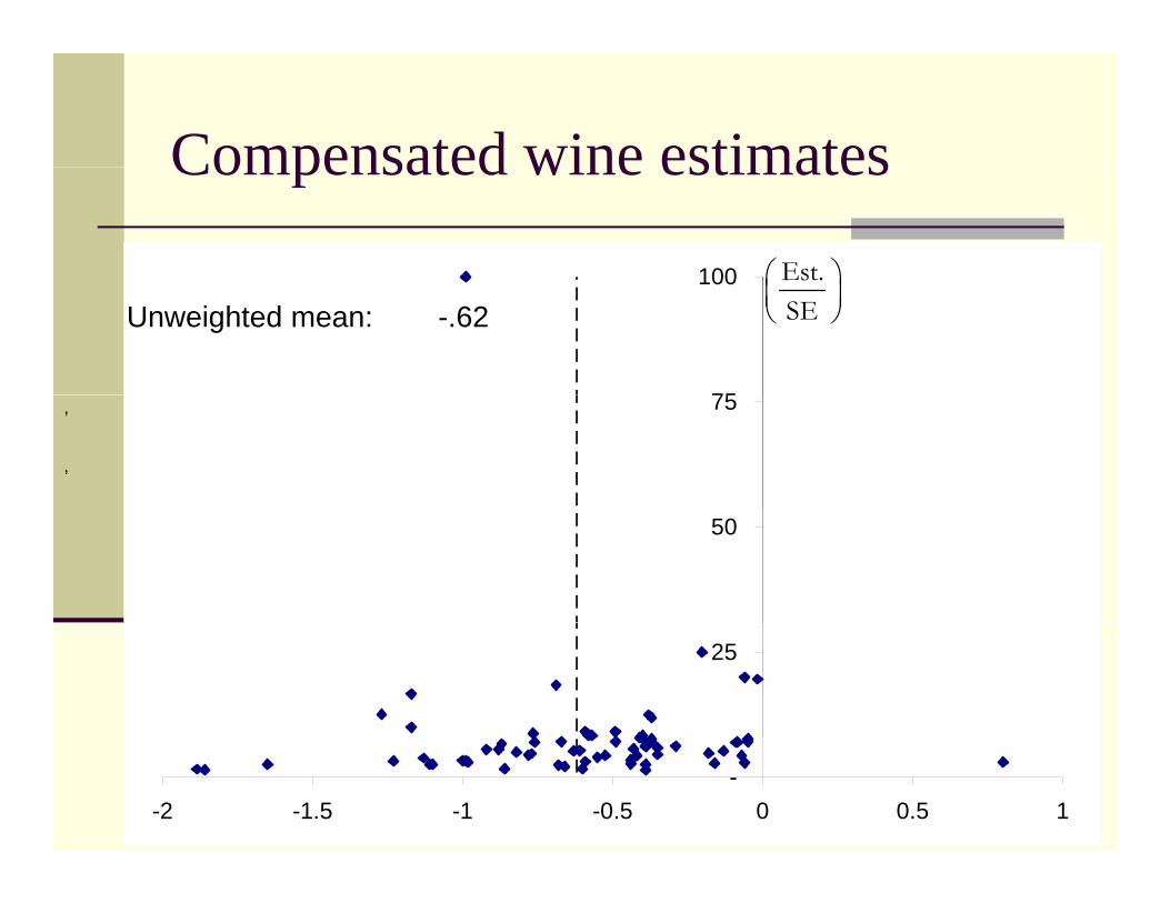
Compensated wine estimatesCompensated wine estimates
,
,

Compensated wine estimates
100
Compensated wine estimates
Est.⎛ ⎞⎜ ⎟100SE
⎛ ⎞⎜ ⎟⎝ ⎠
75,
,
50
25
--2 -1.5 -1 -0.5 0 0.5 1
Compensated wine estimates
100
Compensated wine estimates
Est.⎛ ⎞⎜ ⎟
75
100SE
⎛ ⎞⎜ ⎟⎝ ⎠Unweighted mean: -.62
75,
,
50
25
--2 -1.5 -1 -0.5 0 0.5 1

Compensated wine estimates
100
Compensated wine estimates
Est.⎛ ⎞⎜ ⎟
75
100SE
⎛ ⎞⎜ ⎟⎝ ⎠Unweighted mean: -.62
Fixed effects mean: -.8375
50
25
--2 -1.5 -1 -0.5 0 0.5 1

Compensated wine estimates
100
Compensated wine estimates
Est.⎛ ⎞⎜ ⎟
75
100
Unweighted mean: -.62Fixed effects mean: -.83R d ff t 57
SE⎛ ⎞⎜ ⎟⎝ ⎠
75Random effects mean: -.57
50
25
--2 -1.5 -1 -0.5 0 0.5 1
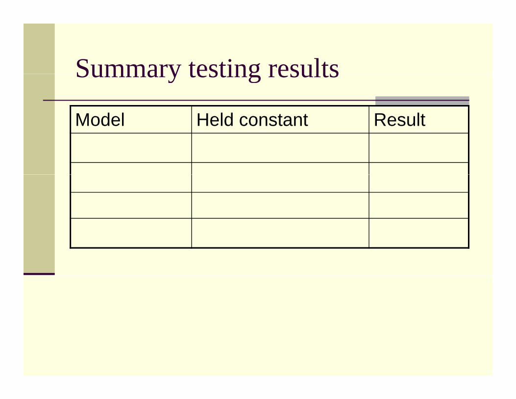
Summary testing resultsSummary testing results
Model Held constant ResultModel Held constant Result

Summary testing resultsSummary testing results
Model Held constant ResultModel Held constant ResultFixed Effects Beverage Always reject
Beverage and country Always rejectBeverage and country Always reject

Summary testing resultsSummary testing results
Model Held constant ResultModel Held constant ResultFixed Effects Beverage Always reject
Beverage and country Always rejectBeverage and country Always reject
Random Effects Beverage Always reject
B d t Al j tBeverage and country Always reject
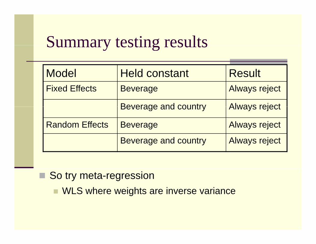
Summary testing resultsSummary testing results
Model Held constant ResultModel Held constant ResultFixed Effects Beverage Always reject
Beverage and country Always rejectBeverage and country Always reject
Random Effects Beverage Always reject
B d t Al j tBeverage and country Always reject
So try meta-regression WLS where weights are inverse variance
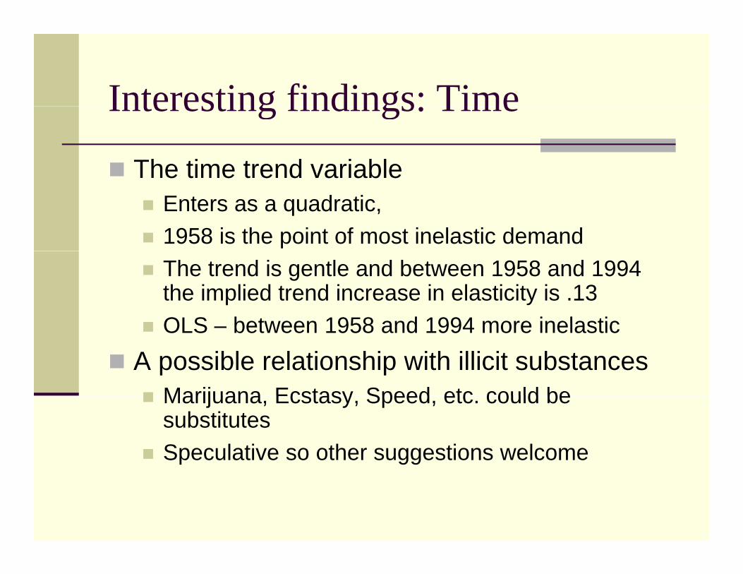
Interesting findings: TimeInteresting findings: Time
The time trend variableEnters as a quadratic,1958 is the point of most inelastic demandThe trend is gentle and between 1958 and 1994 the implied trend increase in elasticity is .13 OLS between 1958 and 1994 more inelasticOLS – between 1958 and 1994 more inelastic
A possible relationship with illicit substancesMarijuana Ecstasy Speed etc could beMarijuana, Ecstasy, Speed, etc. could be substitutesSpeculative so other suggestions welcome

Interesting findings: Country effectsInteresting findings: Country effects
Pair-wise testing – 66 comparisons per beveragePair wise testing 66 comparisons per beverage
Beer Wine Spirits
Average Rejection Rates
Beer Wine Spirits
12 percent 21 percent 12 percent
The main exceptions relate to wine:Wine in France: 73 percent rejection rate (inelastic)Wine in France: 73 percent rejection rate (inelastic)Wine in UK: 45 percent rejection rate (elastic) Wine Canada: 45 percent rejection rate (elastic)Wine Canada: 45 percent rejection rate (elastic)Beer in NZ: 45 percent rejection rate (inelastic)

Final points of noteFinal points of note
Paper available with details and an appendixPaper available with details and an appendix covering each paperThe approach could be a useful framework ppfor some of the hedonic literature on expert opinion etc.