the decision to use alternative payment methods, state...

The Decision to Use Alternative Payment Methods, StateDependence or Unobserved Heterogeneity?

Kim Huynh∗

Department of EconomicsQueen’s UniversityKingston, Ontario

CANADA K7L [email protected]

First Draft: June 12, 2003This Draft: August 25, 2003

Abstract

In recent years interest-bearing checking accounts and ATM cards have become quiteubiquitous. These alternative payment methods offer many benefits, but a majority ofhouseholds have yet to adopt these technologies as a means of payment. The goal of thispaper is to answer why some households have been reluctant to make the switch. Thispaper uses dynamic discrete choice techniques to model household behaviour in adoptingalternative payment technologies. The Bank of Italy’s Survey of Household Income andWealth is used to conduct this study. Preliminary evidence indicates that the householdprevious financial adoption decisions are a major factor in current period adoption choice.

Key Words: Financial Innovation, Discrete-Choice Dynamic Panel Data,JEL Classification: E41, C33

∗The author is grateful to Giovanni D’Alessio for kindly providing the Bank Italy Survey of HouseholdIncome and Wealth dataset. Helpful comments and suggestions from Gregor Smith is greatly appreciated andacknowledged. Many thanks to Katerina Kyriazidou for kindly providing the code for the semiparametricconditional logit estimator and Shannon Seitz for the use of her computer and software. Editorial commentsand suggestions from Vien Huynh greatly improved the readiblity of this paper. Financial support from theSocial Sciences and Humanities Research Council of Canada is gratefully acknowledged. The usual disclaimeron liability applies.

1

1 Introduction

Currency has taken many forms in its history. In 9000 B.C., cattle and crops were used asa form of currency; in 1000 B.C. base metal coins were introduced, then paper money in 800A.D. In the modern age, money has taken on a more sophisticated form. Through technologicalprogress, the use of paper and coin currency has almost become unnecessary. This decision forhouseholds to use alternative methods of payments other than money is commonly referred toas financial innovation. Recent examples of financial innovation are interest-bearing checkingaccounts, credit cards, and ATM cards. The obvious advantage of these payments tools is thatit allows the household to economize on their money holdings while providing liquidity services.A concise and lucid survey of the evolution of payment systems is contained in the book byEvans and Schmalensee (1999).

The introduction of financial innovation has resulted in a significant increase in personal ef-ficiency, reducing the time, and cost, involved with money transactions. A greater benefit hasproven to be the opportunity to circumvent the inflation tax. By depositing money into a bankaccount which pays a nominal interest rate, ensures that money retains its value. Safety is alsoa factor, reducing the amount of cash that is held. Shoe leather costs associated with money arereduced. In addition, issues of counterfeiting and deterioration of money are also avoided. Withthe myriad of benefits associated with financial innovation, why is it that some households arehesitant to adopt financial innovation?

Theoretical studies such as Ireland (1995), Lacker and Schreft (1996), and Uribe (1997) haveshown that episodes of high inflation have spurred on the rate of financial innovation. However,empirical studies such as Gordon, Leeper, and Zha (1998) are unable to match the trends in theaggregate data. One reason for this inadequacy is the assumption that households can smoothlysubstitute between alternative payment methods. The relaxation of this assumption requiresthat the household decisions are made in a sequential order. First the household has to decidewhether to adopt financial innovation or the extensive margin; then conditional on this adoptiondecision the household decides how much to allocate to each payment method or the intensivemargin.

Modelling both the extensive and intensive margins has shed many interesting insights intothe study of monetary economics. As Mulligan and Sala-i-Martin (2000) note in their study;59 percent of U.S. households in 1989 did not have an interest-bearing banking account. Whatcould be the reason for the failure to adopt by a non-trivial segment of the population? Anexplanation put forth by Mulligan and Sala-i-Martin is that the fixed costs of adopting financialinnovation introduce frictions into the participation decision. Using the 1989 cross-section ofthe Survey of Consumer of Finances they find that the fixed costs of adoption, approximately111 USD, are quite low. Another important finding is that half of the interest rate elasticity isdue to the extensive margin. However, this study is incomplete since it only provides a snapshoton the role of fixed costs.

2

A study that adds a temporal component is by Attanasio, Guiso, and Jappelli (2002). Theystudy the role of financial innovation and its effect on money demand in Italy for the period1989 to 1995. Using multiple cross-sections from the Bank of Italy’s Survey of Household Incomeand Wealth (SHIW). Attanasio et al. specify a static specification for the financial innovationdecision and money demand function. The household decision to adopt financial innovation ismodelled using the following static discrete choice model:

w∗i = xiβ + vi,(1)

wi =

{1 if w∗

i > 0,0 if w∗

i ≤ 0.

Where wi is a binary choice variable which takes value of one if the household i has adoptedfinancial innovation, and zero otherwise. The variable xi contains a vector of household charac-teristics such as consumption level, financial wealth, and various demographic factors (education,place of residence, age and sex of head of household). It also contains information on the nom-inal deposit interest rate and number of bank branches in the region that household resides.

The probit estimates are used to form the inverse Mills ratio which are used as the condi-tioning variable in their switching regressions of household money demand; refer to Maddala(1983) for a discussion of this technique. The estimates of the household money demand func-tion are used to quantify the welfare costs of inflation (Bailey triangles), a welfare metric firstdiscussed by Bailey (1956). Other than calculating the direct inflation tax, which is trivial, theyalso calculate the cost of financial innovation borne by households. These costs are included inthe welfare comparison since they are incurred by households in order to aid in the avoidance ofthe inflation tax. They find that adoption costs are quite low, ranging from 14.3 to 28.1 euros.This cost, comparable to direct financial adoption cost, is about 6.2 euros. The direct financialcosts are from a sample of representative Italian banks.

Why do such low trivial financial adoption costs result in such low adoption rates of finan-cial innovation? An explanation of this phenomena focuses on the heterogeneity between thehouseholds. Up to now the studies involving financial innovation use only cross-sectional meth-ods; their is no attempt to follow households across time. For example, studies on householdadoption of alternative payment methods by Stavins (2001) or effect of financial innovation onstock market participation by Reynard (2003) use only multiple cross-sections of the Survey ofConsumer Finances. In alternative fields longitudinal or panel data has proven to be quite fruit-ful approach to investigating household decisions; the field of labour economics has been quitean active research area for panel data. Many sharp and interesting results have been completedwith longitudinal data that refutes the findings of cross-sectional studies. Panel data has beenused in the study by Humphrey, Pulley, and Vesala (1996) to look at cross-country differencesin financial innovation. However, the study of financial innovation using household panel datais still in its infancy.

One of the contributions of this paper is to utilize panel data in the study of financial innova-tion. The SHIW has a panel component but Attanasio et al. ignored this feature of the data

3

and treated the data as one large cross-section. A preliminary study by Huynh (2003) exploitsthe panel component of the SHIW to account for this heterogeneity. This study recalculatessome key summary statistics and estimates the models using static panel data techniques. Aninsight of this study was that major determinants of financial innovation are interest rates, con-sumption, and wealth after controlling for household characteristics such as education, place ofresidence, presence of a male head of household. These finding begs the question, why do poorerhouseholds in Italy have low adoption rates of financial innovation? What is preventing themfrom adopting financial innovation so as to avoid the inflation tax? Answering this questionhas many policy implications. A calibration study by Erosa and Ventura (2002) demonstratesthat when households do not participate on the extensive margin then inflation is a regressivetax. The results are particularly interesting since Italian inflation was quite high (six to eightpercent) in the beginning of the 1990’s.

The static specification is unsatisfying since it ignores the dynamic nature of the decision toadopt financial innovation. Table 1 and 2 summarize the participation sequences of households.The decision to adopt an interest-bearing account and ATM cards are quite persistent processes.Accounting for this persistence involves looking at the issue of state dependence, or how cur-rent behaviour affects future behaviour. The notion of state dependence indicates that currentparticipation directly affects the preferences or opportunities of the household which, in turnaffects future participation.

Although, technological progress has greatly simplified the knowledge required, the cost of learn-ing still remains a nontrivial cost. The panel, which consists of a sample of Italian households,can be used to explore this heterogeneity across households. Apart from the inflation tax; thesevaried fixed costs may explain households reluctance to adopt financial innovation. The dataalso indicates that once households have adopted they will retain their financial innovation bar-ring a shock to their household state.

An alternative explanation to the persistence of these discrete outcomes is that unobservablecharacteristics may affect households behaviour towards financial innovation. For example, ahousehold that engages in illegal activities and/or is active in the underground economy wouldnot adopt financial innovation so as to avoid detection by the legal authorities. Mistrust offinancial institutions could be another reason for the lack of adoption by households.

If the major reason for this persistence is state dependence, then one method for policymakersto ameliorate the effect of the inflation tax is to encourage households to adopt financial innova-tion. If it is unobserved heterogeneity then policies that are aimed at increasing adoption rateswould be ineffective. Therefore, an important task is to disentangle these two effects. Dynamicdiscrete choice panel data models can be used to disentangle these two effects and model thebehaviour households. The use of panel data is particularly appropriate in this case as it con-tains repeated observations of a given group or individuals over time; therefore, their behaviourand choices can be modelled by looking at the differences between households and time.

4

The rest of the paper is organized in the following fashion. Since dynamic discrete choicemodels are quite novel, these techniques are discussed in Section 2. Section 3 looks at a dy-namic model of financial innovation. Section 4 empirically implements the model specificationof financial innovation; dynamic discrete choice models are used to estimate the conditionalprobability that a household will choose to adopt financial innovation. The empirical results arepresented in Section 5. Section 6 concludes with some remarks and some ideas on future work.

2 Dynamic Discrete Choice Panel Data Models

The following discussion is drawn from the following sources Arellano and Honore (2001), Hsiao(2002), and Miniaci and Weber (2002). A dynamic discrete choice panel data model has thefollowing structure:

w∗it = xitβ︸︷︷︸

observables

+ γwi,t−1︸︷︷︸state dependence

+ αi︸︷︷︸unobserved heterogeneity

+ uit︸︷︷︸error term

, i = 1 . . . N, t = 1 . . . T,(2)

wit =

{1 if w∗

it > 0,0 if w∗

it ≤ 0,

where vit = αi + uit.

Where wit denotes the adoption decision of household i in period t; xit is a vector of observablehousehold characteristics; β is the effect of xit on the participation decision; γ is the parameterthat represents the extent of true state dependence (TSD) on the adoption decision. With paneldata, repeated observations of a given group of individuals, the error term vit can be decomposedinto two components: αi is the time-invariant household-specific or unobserved heterogeneity anduit is assumed to be independently distributed over i with a distribution F (·).

Identifying the source of persistence is a challenging task. Persistence in this model arisesfrom three sources:

1. true state dependence,

2. unobserved heterogeneity,

3. error term.

How should a statistically significant coefficient γ 6= 0 be interpreted? Is it really TSD or is itunobserved heterogeneity? The cautious approach is to agree that γ 6= 0, is a necessary, but nota sufficient condition for TSD. To ensure that the correct inference is made, consistent modelestimated are required.

A classic example of this identification problem is the issue of labour supply. Phelps (1972)found that current unemployment spells affected future unemployment spells. This result im-plies that, due to the the effects of state dependence, short-term policies can have a long term

5

impact on alleviating unemployment. However, Cripps and Tarling (1974) argued that unob-servable characteristics were driving individual unemployment spells, not their past behaviour.Concluding that there is true state dependence when it it is really unobserved heterogeneity iscalled spurious state dependence (SSD).

The issue of how to treat the initial conditions of the model exacerbates the identificationproblem. Incorrect handling of the initial condition will yield inconsistent parameter estimates.This is particularly a problem in large N and short T panels. Also, these dynamic discretechoice models are nonlinear, which complicates the estimation method.

In the literature two type of estimators are employed: the fixed effects and random effectsmodels. The choice of estimator is unclear, as each has its merits and weaknesses. For this rea-son, it would be useful to follow the approach of Chay and Hyslop (2000) who consider in detailboth types of estimators. Consequently, a brief discussion these estimators will be provided.

2.1 The Parametric Likelihood and the Random Effects Estimator

The random effects estimator is often referred to as an parametric estimator since it requiresdistributional assumptions for both αi and the initial condition. To assist in the parameterizationof the initial condition the following assumptions can be made:

1. The initial conditions are an exogenous process.

2. The process is in an equilibrium.

The first assumption can be taken seriously when the starting point of the sample is observable.An example of this is the study of labour supply decisions; one observes at the beginning of thesample the decisions of individuals who have just graduated from high school who are enteringthe labour force. The latter assumption is not as attractive, since in many cases the stochasticprocess is being driven by time-varying exogenous variables.

To see how each of the assumptions are treated in the estimation technique, it would be usefulto look at the likelihood functions of each approach.

2.1.1 The Likelihood

Suppose that the dynamic discrete choice model follows a first-order Markov process with noexogenous variables:

w∗it = β0 + γwi,t−1 + vit,(3)

where vit = uit + αi,

wit =

{1 if w∗

it > 00 if w∗

it ≤ 0

6

• Exogenous initial conditions:For this case the joint probability of wit for a given αi is:

T∏t=1

F (wit|wi,t−1, αi) =T∏

t=1

Φ{(β0 + γwi,t−1 + αi)(2wit − 1)}.(4)

Let Φ denote the standard normal cumulative distribution function. If αi is random witha distribution G(α) the likelihood function is:

L =N∏

i=1

∫ T∏t=1

Φ{(β0 + γwi,t−1 + α)(2wit − 1)}dG(α).(5)

• Equilibrium process:For this case the the limiting marginal probabilities are:

wi0 = 1 with Pi =Φ(β0 + αi)

1− Φ(β0 + γαi) + Φ(β0 + αi)

wi0 = 0 with 1− Pi =1− Φ(β0 + γαi)

1− Φ(β0 + γαi) + Φ(β0 + αi).

Therefore the joint probability of wit for a given αi is:

T∏t=1

Φ{(β0 + γwi,t−1 + α)(2wit − 1)} × Pwi0i (1− Pi)

1−wi0 .(6)

The likelihood function for the random effects is:

L =N∏

i=1

∫ T∏t=1

Φ{(β0 + γwi,t−1 + α)(2wit − 1)} × Pwi0i (1− Pi)

1−wi0dG(α).(7)

With the random-effects the maximum likelihood estimates (MLE) of β0, γ, and σ2α are consistent

if either N →∞ or both N or T →∞. The weakness of the likelihood approach is that if theparametric assumptions can be rejected, the estimates will be inconsistent. To avoid inconsistentestimators when the above initial conditions assumptions fail, less restrictive likelihoods will haveto be specified.

2.1.2 Intractable Likelihoods

In the event that neither of the assumptions hold; the of relationship between wi0 and αi mustbe considered. The likelihood for the random-effects model is:

L =N∏

i=1

∫ ∞

−∞

T∏t=1

F (wit|wi,t−1, α)f(wi0|α)dG(α).(8)

7

An even more complicated likelihood would be to introduce a fixed-effects model so that:

L =N∏

i=1

T∏t=1

Φ{(β0 + γwi,t−1 + αi)(2wit − 1)}f(wi0|αi).(9)

Where f(wi0|α) is the marginal probability of wi0 given αi. Finding a closed-form expression forthis marginal probability is non-trivial. Maximizing such a likelihood can be computationallyexpensive. One could overcome the complexity of the likelihood by using simulation techniques,for example see Lee (1997). Alternatively, Bayesian and Markov-Chain Monte-Carlo methodscan be used to obtain a exact estimators, an example of this approach is McCulloch and Rossi(1994).

2.1.3 Heckman’s Approximate Method

If the initial conditions assumptions or alternative simulation-based methods are not palatable,an approximation method can be employed. Heckman (1981b) suggests such a method to dealwith the initial conditions problem. The method can be broken down into the following threesteps

1. Approximate the initial condition, wi0 by estimating the following probit model with angeneral index Q(xi):

w∗i0 = Q(xi) + εi0

wi0 =

{1 if w∗

i0 > 00 if w∗

i0 ≤ 0

2. Allow εi0 to be correlated with vit with t = 1 . . . T .

3. Maximize the likelihood and obtain an estimate of the model without any restrictionsbetween the structural parameters and approximated initial conditions.

Heckman provides Monte Carlo evidence that this approximate random-effects estimator issuperior to the fixed-effects model. However, the estimators are still biased in small samples.Nevertheless, this method is quite easy to implement.

2.2 The Conditional Logit or Fixed-Effects Estimator

The random-effects/parametric likelihood will yield inconsistent estimates if the individual ef-fects are indeed fixed. This assumption can be tested using a Durbin-Wu-Hausman test. If therandom effects model is rejected, then, the fixed-effects can be employed.

An alternative to the parametric likelihood/random-effects method is the conditional approachdiscussed by Chamberlain (1993) and generalized by Honore and Kyriazidou (2000). The con-ditional approach is quite technical; interested readers are advised to consult these referencesdirectly. The main idea behind this method is to concentrate the fixed-effects (αi) out of thelikelihood. The approach involves assuming a logistic distribution for the error terms (uit),therefore completing the term conditional logit.

8

2.2.1 Conditional Logit

Chamberlain (1993) shows that when T ≥ 3 the parameters β and γ can be estimated indepen-dent of αi. T refers to the number of usable data points excluding the initial condition. Supposethe model of (yi0 . . . yiT ) is of the form:

P (wi0 = 1|αi) = P0(αi),(10)

P (wit = 1|αi, wi0 . . . wi,t−1) =exp(γwi,t−1 + αi)

1 + exp(γwi,t−1 + αi), t = 0, 1, 2, . . . T.(11)

The following discussion looks at the simplest case when T = 3. Consider the following se-quences:

A = {wi0, wi1 = 1, wi2 = 0, wi3},B = {wi0, wi1 = 0, wi2 = 1, wi3},

where the initial and terminal condition (wi0 and wi3) are allowed to vary (either 1 or 0). Thesequences (wi0, 0, 0, wi3) or (wi0, 1, 1, wi3) are not considered because these events do not helpidentify changes in states. The probabilities of each event are:

P (A) = P0(αi)wi0 [1− P0(αi)]

1−wi01

1 + exp(γwi,0 + αi)

exp(αi)

1 + exp(αi)

exp[(γ + αi)wi3]

1 + exp(γ + αi),(12)

P (B) = P0(αi)wi0 [1− P0(αi)]

1−wi0exp(γwi,0 + αi)

1 + exp(γwi,0 + αi)

1

1 + exp(αi)

exp(αiwi3)

1 + exp(αi).(13)

The conditional probabilities are then:

P (A|A ∪B) = P (A|wi0, wi1 + wi2 = 1, wi3)(14)

=exp(γwi3)

exp(γwi3) + exp(γwi0)

=1

1 + exp[γ(wi0 − wi3)]

P (B|A ∪B) = P (B|wi0, wi1 + wi2 = 1, wi3)(15)

= 1− P (A|A ∪B)

=exp[γ(wi0 − wi3)]

1 + exp[γ(wi0 − wi3)]

Notice that the conditional probabilities (14) and (15) are no longer depend on the fixed-effectαi. The log-likelihood is similar in form to the conditional logit discussed by Chamberlain(1993):

log L =N∑

i=1

1(wi1 + wi2 = 1)× {wi1[γ(wi0 − wi3)]− log[1 + exp γ(wi0 − wi3)]}.(16)

9

2.2.2 Semiparametric Conditional Logit Estimator

The method described by Chamberlain (1993) does not include exogenous variables (xit). Oncexit is added, the likelihood is more complicated because the conditional probabilities are nolonger independent of αi. To deal with this problem Honore and Kyriazidou (2000) make afurther restriction that xi2 = xi3 so that:

P (A|A ∪B, xi, αi, xi2 = xi3) =1

1 + exp[(xi2 − xi3)′β + γ(wi0 − wi3)].(17)

In most cases, especially with continuous variables, xi2 6= xi3 so the log-likelihood is modifiedinto the following form:

N∑i=1

1(wi1 + wi2 = 1)K

(xi2 − xi3

σN

)log

{exp[(xi2 − xi3)

′b + γ(wi0 − wi3)]wi1

1 + exp[(xi2 − xi3)′b + γ(wi0 − wi3)]

}.(18)

The kernel density function, K(·), is introduced in order to give more weight to observations forwhich xi2 is close to xi3. For the formulation of the more generalized the case, T > 3, pleaserefer to Honore and Kyriazidou (2000).

One of the major advantages of the conditional approach is that the problem of initial con-ditions does not have to be modelled explicitly. Also, assumptions are not required for therelationship between the individual effects, explanatory variables, and initial condition. Thedisadvantage is the requirement that xi2 = xi3; as a result some explanatory variables such astime dummies cannot be used. When Honore and Kyriazidou (2000) propose to replace this

restriction with a kernel density estimator the rate of convergence is lower n−13 i.e. more data

is required for the asymptotics to hold. Another disadvantage is that the individual effect arenot estimated therefore it is not possible to calculate elasticities or make predictions with themodel.

2.3 A Simple Test for State Dependence

These estimators discussed have been discussed to quantify the extent of state dependence andunobserved heterogeneity. A simple test has been suggested by Chamberlain (1978) to test forthe presence of state dependence. Chamberlain makes the following observation: the differencebetween TSD versus SSD is whether the dynamics are due to a policy intervention. γ = 0implies that changes in xit will affect wit immediately; but if γ 6= 0 then changes in xit will havea distributed lag affect on wit. A simple test for TSD could be:

TSD : P (wit = 1|xi,t, xi,t−1, . . . , αi) = P (wit = 1|xit, αi),(19)

SSD : P (wit = 1|xi,t, xi,t−1, . . . , αi) 6= P (wit = 1|xit, αi).(20)

This test can be implemented by estimating the following relationship:

w∗it = xitβ + φ(L)xit + αi + uit,(21)

wit =

{1 if w∗

it > 0,0 if w∗

it ≤ 0,

10

If the lag structure, φ(L), is statistically significant then there is some evidence of TSD.

3 A Model of Financial Innovation

Households make consumption/savings decision subject to an intertemporal budget constraintaugmented with a transactions cost function. The transactions costs are increasing in consump-tion and decreasing in money balances. The role of money is to lower transactions cost. The costof holding money is that it is subject to an inflation tax. To avoid the inflation tax householdscan choose to pay a fixed cost in order to adopt financial innovation such as an interest-bearingbank account. The total opportunity cost of using money is the foregone real return on inter-est plus any inflation tax. Therefore, households must make the following discrete/continuousdecisions:

1. Extensive margin - this discrete decision determines whether or not to adopt financialinnovation,

2. Intensive margin - conditional on the discrete choice this continuous decision involveschoosing the optimal portfolio of the household.

A dynamic optimization approach is required to solve such a problem.

3.1 Dynamic Optimization Problem

The household optimization problem is to maximize the following utility function:

max Ut =∞∑

t=0

δtEtu(ct),(22)

subject to the following budget constraint:

at+1 = φtat + ht(1− φt)(1 + rt)at + yt − ct − s(φtat, ct)(23)

− (πtφt−1at)(1− ht−1)−max[(ht − ht−1)κ, 0].

Where ct is consumption and δ is the discount rate. ht is the binary choice variable which takesvalue one if the household has adopted financial innovation otherwise it is equal to zero. Theamount of assets that household brings into time t is at; while φt is the share of the asset heldas money and (1 − φt) is the fraction held in a bank account, rt is real return of the bankaccount, yt is exogenous stream of labour income, πt is the inflation rate, and κ is the fixed costof financial adoption. The term πtφt−1at is the amount of inflation tax that household incursby not adopting financial technology. The transaction technology or shopping cost function,s(φtat, ct), has the following properties:

s(φtat, ct) ≥ 0, s(φtat, 0) = 0,

s1(φtat, ct) ≤ 0, s2(φtat, ct) ≥ 0,

s11(φtat, ct) ≥ 0, s22(φtat, ct) ≥ 0, s12(φtat, ct) ≤ 0.

11

3.2 Dynamic Programming Problem

The value function depends on the following state variables: previous choices on whether toadopt financial innovation (ht−1), previous portfolio weights (φt−1), amount of assets broughtinto the current time period (at), and observable household state or characteristics (Zt). House-hold control or choice variables are then: consumption (ct) and savings (at+1), financial innova-tion (ht), and current portfolio weights (φt).

The Bellman equation at time t is:

V (ht−1, φt−1, at, Zt) = max[V 0(ht−1, φt−1, at, Zt), V1(ht−1, φt−1, at, Zt)],(24)

where superscript 0 and 1 denote the period t no-adopt and adopt states. To gain some insightinto the problem lets consider the following cases: First, households who have not adoptedfinancial innovation must decide whether to pay the fixed cost κ in order to adopt financialinnovation; Second, households who have adopted financial innovation must make the decisionwhether to keep on using such financial innovation. To elucidate these problems look at thehousehold dynamic programming in the two possible states.

3.2.1 Households who did not adopt financial innovation

The dynamic program for a household that has not adopted financial innovation in period t− 1is:

V (0, 1, at, Zt) = max[V 0(0, 1, at, Zt), V1(0, 1, at, Zt)].(25)

The household will adopt financial innovation if V 0(0, 1, at, Zt) < V 1(0, 1, at, Zt), or:

u[at + yt − at+1 − s(at, ct)− πtat, 0, Zt] + δEtV (0, 1, at, Zt+1)︸︷︷︸did not adopt financial innovation

<(26)

u[φtat + (1− φt)(1 + rt)at + yt − at+1 − s(φtat, ct)− πtat − κ, 1, Zt] + δEtV (1, 1, at, Zt+1)︸︷︷︸did adopt financial innovation

.

Rearranging so as to compare current utility versus future expected utility yields:

u[φtat + (1− φt)(1 + rt)at + yt − at+1 − s(φtat, ct)− πtat − κ, 1, Zt]

− u[at + yt − at+1 − s(at, ct)− πtat, 0, Zt] > δ[EtV (0, 1, at, Zt+1)− EtV (1, 1, at, Zt+1)].

Inverting these monotonic utility functions then approximating the difference yields:

rtat(1− φt) + s(φtat, ct)− s(at, ct)− k > ϕ{(δEt[V (0, 1, at, Zt+1)− V (1, 1, at, Zt+1)]}−1,(27)

or

rtat(1− φt) + s(φtat, ct)− s(at, ct)︸︷︷︸benefit of having adopted financial innovation

> k + ϕ{δEt[V (0, 1, at, Zt+1)− V (1, 1, at, Zt+1)]}−1

︸︷︷︸fixed adoption cost+Difference in expected future utility

.

12

3.2.2 Households who did adopt financial innovation

The dynamic program for household who has adopted financial innovation in period t− 1 is:

V (1, φt−1, at, Zt) = max[V 0(1, φt−1, at, Zt), V1(1, φt−1, at, Zt)].(28)

The household will keep using their financial innovation if V 0(1, φt−1, at, Zt) < V 1(1, φt−1, at, Zt|ω1)or:

u[at + yt − at+1 − s(at, ct), 0, Zt] + δEtV (0, φt−1, at, Zt+1)︸︷︷︸Un-adopt financial innovation

<(29)

u[φtat + (1− φt)(1 + rt)at + yt − at+1 − s(φtat, ct), 1, Zt] + δEtV (1, φt−1, at, Zt+1)︸︷︷︸Retain financial innovation

.

Similar derivation yields the following condition for households to keep their bank account:

rtat(1− φt) + s(φtat, ct)− s(at, ct)︸︷︷︸Benefit of Retaining financial innovation

>(30)

ϕ{δEt[V (0, φt−1, at, Zt+1)− V (1, φt−1, at, Zt+1)]}−1

︸︷︷︸Difference in expected utility

.

4 Empirical Specification and Estimation

The previous sections have discussed the econometric issues involved with estimating dynamicdiscrete choice models and laid the framework for a model of financial innovation. This sectioncasts the model of financial innovation into an econometric framework, using the choices ofItalian households in the SHIW. This approach has previously been used by Hyslop (1999) tolook at female labour participation rates.

4.1 Theory Taken to the Data

The value functions (25) and (28) describe the behaviour of households. The decision to adoptfinancial innovation is a function of:

1. Consumption (ct)

2. Financial Wealth (at)

3. Interest rate (rt)

4. Fixed cost of setting up bank account (κ)

5. Previous state of the household choices (ht−1, φt−1)

6. Household characteristics (Zt)

13

The decision to adopt financial innovation, checking account or an ATM card, is modelled usinga dynamic binary choice model. The empirical specification is of the form described in (2):

wit = 1{xitβ + γwi,t−1 + αi + εit},

where wit is a binary variable that takes value 1 if household has adopted that form of financialinnovation and zero otherwise. The observable variables, xit, are: consumption (logc), financialwealth (logfinw), interest rate (logr), and household characteristics.

The household characteristics variables are introduced to control for differences in households.These variables consist of:

1. Education level for the head of the household (educ); dummy variables with four controls.

2. Where does the household reside (live); dummy variable with three controls.

3. Whether the head of household is male (malehead); equal to 1 if male 0 otherwise.

4. Age of the head of household (eta); continuous variable.

Tables 1, 2, and 3 summarize the characteristics of these variables. The balanced panel consistsof 1236 households but for estimation purposes, only 1234 household observations are used. Twohouseholds are excluded because their financial wealth is unreported in 1991.

To control for the supply of financial innovation, the number of bank branches in the region thehousehold resides is included (logQ). At the present time there is no data on the cost structureof the financial industry, or a technological change; as a result, a quadratic time trend is addedto proxy for these processes. The fixed cost, κ, is unobserved so it cannot directly estimated,but it is assumed that αi captures part of this term. For a detailed explanation of the variablesplease refer to the Appendix.

4.2 Estimation Techniques

The estimation and inference strategy is similar in spirit to that of Hyslop (1999) and Chinta-gunta, Kyriazidou, and Perktold (2001). The general test for TSD suggested by Chamberlain(1978) will be implemented. Next the parameters of the discrete choice models are estimatedusing the following estimators: Heckman (1981b) approximate random-effects (HRE), a probitrandom-effects (XTRE), a fixed-effects conditional logit (XTFE), and theHonore and Kyriazi-dou (2000) semiparametric fixed-effects conditional logit (HK). Since the HK estimator relies onkernel smoothing five different bandwidths are presented. Another feature of the HK estimatoris that it has less conditioning variables than the other estimators. The reason for this feature isto avoid the curse-of-dimensionality problem related with kernel smoothing multivariate modelsand time-variant variables such as time dummies are not allowed.

14

5 Results

The participation sequences are calculated for household adoption of interest-bearing bank ac-count, bank account conditional on not having an ATM, and ATM card. The results aresummarized in Table 1; a striking feature of this table is the segmentation between the twogroups. The full participation sequences for households with bank accounts is quite high - 984out of possible 1234 or about 80% households always had a bank account. For the ATM casethere are two large groups the full adopters (322) versus non adopters (407). Another case isthe group of households who adopted post-1995 (95).

To attempt to control for the possible stepwise decision, the participation sequences are cal-culated for households who have always had a bank account in all five periods (984); the resultsare summarized in Table 2. This table indicates that out of possible 984 households 322 haveadopted an ATM card never gave it up. Also, 223 households or about 23% who had an interest-bearing checking account never adopted an ATM card at all. These results indicate that thereis some evidence of state-dependence.

To test this empirically the binary choice models are applied to three different classifications:

1. Check: household who have adopted interest-bearing bank accounts,

2. ATM: households who have adopted ATM cards,

3. CATM: households who have adopted ATM cards conditional on having a bank accountin all five periods.

The first step is to apply the test for TSD suggested by Chamberlain (1978). Results are sum-marized in Table 6 and point to evidence that it is TSD since the coefficients of the laggedindependent terms are statistically significant.

The next step is to estimate the binary choice models for each of the three different deci-sions. The results of these estimates are summarized in Table 7, 8, and 9. For the check caseboth the random-effects estimator, HRE and XTRE, indicate that there is strong evidence ofpositive state dependence. However, the XTFE indicates that γ is negative and is not statis-tically different from zero. This result implies that there is no state dependence. However,the HK estimator confirms the results of the random-effects estimator since for all bandwidthparameters γ is statistically significant. Another interesting observation is that the estimatedparameters from the fixed-effect have larger standard errors than the random-effects estimators.This implies that household differences do not have much explanatory power in the fixed-effectsmodels.

For the ATM and CATM cases the conclusion is the same as the Check case; the random-effectsand HK estimator indicate that state dependence is statistically significant while the XTFEshows that γ is statistically insignificant. Also, the parameter estimates from the random-effects estimator are much sharper than the fixed-effects model. It seems that conditioning on

15

households who always had a bank account did not really change the results; as the coefficientsfrom both state dependence equations are roughly the same. The only difference seems to bethe effect of interest rates and financial wealth on the decision to adopt. For the CATM case,these variables were lesser in magnitude than the ATM case.

6 Conclusions

The result of the dynamic discrete models indicate that there is evidence that the decision toadopt financial innovation displays true state dependence. This implies that past household de-cisions to adopt financial innovation play a role in current household decision to adopt financialinnovation. This result concurs with the data. From the participation sequences, a large numberof households who have adopted financial innovation keep it and never switch out. Householdswho did not adopt financial innovation tend to stay in this state.

However, it is unsettling that the econometric evidence is not overwhelming. The fixed-effectsconditional logit clearly indicates that there is no state dependence. This conflict conclusionneeds to be reconciled. Monte Carlo studies by Chintagunta, Kyriazidou, and Perktold (2001)have found that the fixed-effect conditional logit models are negatively biased towards zero. Anatural extension is to use the actual design matrix of this problem and conduct a Monte-Carlostudy. Alternatively, more complicated estimators can be considered. In the case of Chay andHyslop (2000) the authors use simulation-based estimators with much more complicated errorstructures. Another complication that one can consider is to model the stepwise decision pro-cess; a bank account is a necessary condition for an ATM card. It maybe fruitful to look atdynamic discrete nested logit models. Finally these reduced-forms methods might not be able todistinguish between the state dependence and unobserved heterogeneity. A natural extension isto consider Markov decision process methods advocated by Rust (1987), Hotz and Miller (1993),and Aguirregabiria and Mira (2002).

16

References

Aguirregabiria, V., and P. Mira (2002): “Swapping the Nested Fixed Point Algorithm: AClass of Estimators for Discrete Markov Decision Models,” Econometrica, 70(4), 1519–1543.

Arellano, M., and B. Honore (2001): Handbook of Econometrics vol. 5, Chapter 53: PanelData Models: Some Recent Developments, pp. 3229–3296. Elsevier.

Attanasio, O. R., L. Guiso, and T. Jappelli (2002): “The Demand for Money, FinancialInnovation, and the Welfare Cost of Inflation: An analysis with Household Data,” Journal ofPolitical Economy, 110(2), 317–351.

Bailey, M. J. (1956): “The Welfare Costs of Inflationary Finance,” Journal of Political Econ-omy, 64, 93–110.

Brandolini, A., and L. Cannari (1994): Saving and the accumulation of wealth : essays onItalian household and government saving behavior Chapter Methodological Appendix: TheBank of Italy’s Survey of Household Income and Wealth. Cambridge University Press.

Chamberlain, G. (1978): “On the Use of Panel Data,” paper presented at the Social ScienceResearch Council Conference on the Life-Cycle Aspects of Employment and the Labor Market,Mt. Kisco, N.Y.

(1993): “Feedback in Panel Data Models,” mimeo. Department of Economics, HarvardUniversity.

Chay, K., and D. Hyslop (2000): “Identification and Estimation of Dynamic Binary Re-sponse Panel Data Models: Empirical Evidence Using Alternative Approaches,” unpublished.

Chintagunta, P. K., E. Kyriazidou, and J. Perktold (2001): “Panel Data Analysis ofHousehold Brand Choices,” Journal of Econometrics, 103, 111–153.

Cripps, T., and R. Tarling (1974): “An Analysis of the Duration of Male Unemploymentin Great Britain, 1932-1973,” Economic Journal, 84, 289–316.

Erosa, A., and G. Ventura (2002): “On Inflation as a Regressive Consumption Tax,”Journal of Monetary Economics, 49, 761–795.

Evans, D. S., and R. Schmalensee (1999): Paying with Plastic: The Digital Revolution inBuying and Borrowing. MIT Press.

Gordon, D. B., E. M. Leeper, and T. Zha (1998): “Trends in Velocity and Policy Expec-tations,” Carnegie-Rochester Conference Series in Public Policy, 49, 265–304.

Heckman, J. J. (1981b): Structural Analysis of Discrete Data with Econometric ApplicationsChapter Four: The Incidental Parameters Problem and the Problem of Initial Conditions inEstimating a Discrete Time-Discrete Data Stochastic Process, pp. 179–195. MIT Press.

17

Hester, D. D., G. Calcagnini, and R. de Bonis (2001): “Competition through Innovation:ATMs in Italian banks,” Rivista Italiana degli Economisti, (3), 359–381.

Honore, B. E., and E. Kyriazidou (2000): “Panel Data Discrete Choice Models withLagged Dependent Variables,” Econometrica, 68(4), 839–74.

Hotz, V., and R. Miller (1993): “Conditional Choice Probabilities and the Estimation ofDynamic Models,” Review of Economic Studies, 60(3), 497–531.

Hsiao, C. (2002): Analysis of Panel Data. Cambridge University Press.

Humphrey, D. B., L. B. Pulley, and J. M. Vesala (1996): “Cash, Paper, and ElectronicPayments: A Cross-Country Analysis,” Journal of Money, Credit, and Banking, 28(4), 914–939.

Huynh, K. P. (2003): “Money Demand and Financial Innovation: A Dynamic Microecono-metric Approach,” mimeo.

Hyslop, D. (1999): “State Dependence, Serial Correlation and Heterogeneity in IntertemporalLabor Force Participation of Married Women,” Econometrica, 67, 1255–1294.

Ireland, P. (1995): “Endogenous Financial Innovation and the Demand for money,” Journalof Money Credit and Banking, 27, 107–123.

Lacker, J., and S. L. Schreft (1996): “Money and credit as means of payment,” Journalof Monetary Economics, 38(1), 3–23.

Lee, L.-F. (1997): “Simulated Maximum Likelihood Estimation of Dynamic Discrete ChoiceStatistical Models: Some Monte Carlo Results,” Journal of Econometrics, 82, 1–35.

Maddala, G. (1983): Limited Dependent and Qualitative Variables in Econometrics. Cam-bridge University Press.

McCulloch, R. E., and P. P. Rossi (1994): “An exact likelihood analysis of the multinomialprobit model,” Journal of Econometrics, 64, 207–240.

Miniaci, R., and G. Weber (2002): Household Portfolios Chapter Four: Econometric Issuesin the Estimation of Household Portfolios. MIT Press.

Mulligan, C. B., and X. Sala-i-Martin (2000): “Extensive Margins and the Demand forMoney at Low Interest Rates,” Journal of Political Economy, 108(5), 961–991.

Phelps, E. (1972): Inflation Policy and Unemployment Theory: The Cost Benefit Approachto Monetary Planning. London: Macmillan.

Reynard, S. (2003): “Financial Market Participation, Wealth, and the Extensive Margins ofMoney Demand,” mimeo.

18

Rust, J. (1987): “Optimal Replacment of GMC Bus Engines: An Empirical Model of HaroldZurcher,” Econometrica, 55(5), 999–1033.

Stavins, J. (2001): “Effect of Consumer Characteristics on the Use of Payment Instruments,”New England Economic Review, 3, 19–31.

Uribe, M. (1997): “Hysteresis in a Simple Model of Currency Substitution,” Journal of Mon-etary Economics, 40, 185–202.

19

A Appendix

A.1 Data

The dataset is the Italian Survey of Household Income and Wealth (SHIW) constructed by theBank of Italy. The data is collected as part of the Bank of Italy Historical Database of theSurvey of Italian Household Budgets from 1977-2000. The database contains information on:

• Individual characteristics and occupational status,

• Sources of household income,

• Consumption expenditures,

• Housing information,

• Household financial assets and liabilities.

These surveys were conducted on an annual basis from 1977 to 1984 then 1986. It was thenconducted bi-annually from 1987 to 2000 (replacing 1997 with 1998). Since 1987 some of thehouseholds were re-interviewed in order to introduce a longitudinal aspect to the survey. Thefollowing table summarizes the composition of households in each of the survey:

Bank of Italy: Survey of Household Income and WealthHousehold Participation in Survey

1987 1989 1991 1993 1995 1998 20001987 8,027 1,206 350 173 126 85 611989 7,068 1,837 877 701 459 3431991 6,001 2,420 1,752 1,169 8321993 4,619 1,066 583 3991995 4,490 373 2451998 4,478 1,9932000 4,128

N 8,027 8,274 8,188 8,089 8,135 7,147 8,001

For example, of the 8,001 households that made up the sample in 2000 survey, 61 had partici-pated since 1987, 343 since 1989, 832 since 1991, 399 since 1993, 245 since 1995 and 1,993 since1998. The remaining 4,128 were being interviewed for the first time in 2000.

To accurately represent Italy, the survey employs a two-stage sampling method. In the firststage municipalities are sampled from the area of interest with probability proportional to itssize. In the second stage households are drawn with a probability that is commensurate to itssize. The survey is conducted with the head of the household and involves a computer assistedpersonal interview, commonly known as CAPI. Interested readers are directed to Brandoliniand Cannari (1994) for more a discussion of sample design. External users are provided sampleweights but no information on strata or cluster. Therefore, the following caveat is placed on any

20

statistics calculated using sample weights; the point estimates will be precise but the samplestandard errors will be smaller than the standard errors that condition on the strata or cluster.

The questions regarding assets and liabilities is quite difficult to elicit for two reasons. First,respondents might not want to reveal their wealth. This problem is exacerbated at the extremeleft and right tail of the wealth distribution. Second, respondents might not have an accuratemeasure of their wealth at the time of the interview. To take into account of this problem theinterviewer first asks if the household is involved in any of the following categories - savings,bonds, mutual funds, equities, etc. After these questions are elicited the method of unfoldingbrackets is employed. Households are shown a set of range cards that have numerical values towhich they are asked to choose the card that most appropriately fits them. In recent 1998 and2000 survey the interviewer will attempt to ask for the exact amount. If the household does notrespond they are asked if the exact amount closer to the upper or lower bound.

The interest data is drawn from the Bank of Italy public database available at:

http://bip.bancaditalia.it/4972unix/homebipeng.htm

The banking concentration data was drawn from a special survey from the Bank of Italy madeavailable by Giorgio Calcagnini. More information on its characteristics is available in Hester,Calcagnini, and de Bonis (2001).

A.2 Definitions

Stock variables such as currency-related, deposits, financial wealth, and consumption are ex-pressed in 2000 lire and then converted to euros. The price deflator (13699BVRZF) and lire/euroexchange rate (136..EA.ZF...) is taken from the IMF/IFS database.

• Bank account: The questionnaire asks the household “In the survey year did you or anyother member of your houshold have a bank account?” This binary variable takes thevalue one if the respondent has an account. An account is defined as either a checking,savings, or post office account.

• ATM card: The questionnaire asks the household “Did you or any other member of yourhoushold have an ATM card?”

• Currency: The questionnaire asks the household “What sum of money do you usually havein the house to meet household needs?”

• Minimum amount of currency: The questionnaire asks the household “How much moneydo you usually have in the household when you decide to withdraw more?”

• Number of withdrawals and average withdrawal at an ATM: The questionnaire asks thehousehold “On average, how many withdrawals were made per month during the surveyyear using an ATM card?” and “What was the average amount?”

21

• Number of withdrawals and average withdrawal at the Bank/Post Office: The questionnaireasks the household “On average, how many withdrawals were made per month at the bankor post office, exclude trips to the at the ATM?” and “What was the average amount?”

• Consumption: consists of non-durable consumption which is the total sum of expenditureon food, entertainment, education, clothes, medical expenses, renovations, and imputedrents.

• Deposits: Total deposits in checking accounts, savings accounts, and postal deposits.

• Financial wealth: Deposits + equities + bonds + mutual funds. Both deposits and andfinancial wealth are approximated since the questionaire answer ask households to putthemselves into 15 bands. The level is taken as the average of the upper and lower band.

• Fraction of income received in currency or direct deposit: The questionnaire asks thehousehold “Putting the total value of amounts received during the year equal to 100, whatpercentage was received in the form of...?”

• Education: Households were asked what was the highest education they attained. Theyplaced themselves into six categories:

1. None,

2. Elementary school,

3. Junior high school,

4. High school,

5. Bachelor’s degree,

6. Post-graduate experience.

In the survey the number of individuals with post-graduate experience is quite low andtherefore is amalgamated with bachelor’s degree.

• Place of Residence: Households were asked where their dwelling is located. Householdswere given four categories to choose from:

1. Rural Area,

2. Suburbs,

3. Semi-Center,

4. Center.

• Interest rates: Since, there is no contiguous source that spans the time period 1991 to2000; the interest data was constructed from two sources.

22

TABLE TDC20012

NOMINAL DEPOSIT RATES - DISTRIBUTION BY BRANCH LOCATION (REGION) AND

TYPE OF DEPOSIT

Sample: 1995Q1 to 2002Q3

VOCESOTVOC PHENOMENA OBSERVED

035001039 SAVINGS CERTIFICATES AND CDS

035001037 SIGHT CURRENT ACCOUNT DEPOSITS

035001036 SIGHT SAVINGS DEPOSITS

035001040 TIME CURRENT ACCOUNTS

035001038 TIME DEPOSITS

035001041 TOTAL DEPOSITS

TABLE TDB20620

NOMINAL DEPOSIT RATES ON SAVINGS DEPOSITS - DISTRIBUTION BY BRANCH

LOCATION (REGION) AND SIZE OF DEPOSIT - SAMPLE OF BANKS RAISING

SHORT-TERM FUNDS

Sample: 1989Q4 to 1997Q4

CLASSE_PARZ SIZE OF PARTIAL DEPOSITS

25 1 BILLION LIRE AND MORE (516457 EUROS AND MORE)

23 FROM >= 51646 TO < 129114 EUROS

04 FROM >= 129114 TO < 258228 EUROS

22 FROM >= 25823 TO < 51646 EUROS

24 FROM >= 258228 TO < 516457 EUROS

21 LESS THAN 25823 EUROS

16 TOTAL

A series was constructed from these two samples in the following fashion:

Rjt =

OLDjt if t ∈ [1990Q1, 1994Q4],

12(OLDjt + NEWjt) if t ∈ [1995Q1, 1997Q4],

NEWjt if t ∈ [1998Q4, 2002Q3],

where

OLDjt ≡ TDB20620 : CLASSE PARZ = 16,

NEWjt ≡ TDC20012 : V OCESOTV OC = 035001038.

The series were chosen by minimizing a loss function based on the mean and variance ofthe spread. Subscript j refers to the region that the interest rate was drawn from. Thefollowing table summarizes the 20 regions in Italy; IREG and PVDIP are the SHIW andBank of Italy region identifier and AREA5 is the identifier for the five major areas.

23

REGION IREG PVDIP AREA5 PVDIPPIEDMONT 1 10010 NW 20001VALLE D’ AOSTA 2 10012 NW 20001LOMBARDY 3 10016 NW 20001TRENTINO-ALTO ADIGE 4 10018 NE 20002VENETO 5 10020 NE 20002FRIULI-VENEZIA GIULIA 6 10022 NE 20002LIGURIA 7 10014 NW 20001EMILIA-ROMAGNA 8 10024 NE 20002TOSCANA 9 10028 CENTRE 20003UMBRIA 10 10030 CENTRE 20003MARCHE 11 10026 CENTRE 20003LAZIO 12 10032 CENTRE 20003ABRUZZI 13 10036 SOUTH 20004MOLISE 14 10038 SOUTH 20004CAMPANIA 15 10034 SOUTH 20004PUGLIA 16 10040 SOUTH 20004BASILICATA 17 10042 SOUTH 20004CALABRIA 18 10044 SOUTH 20004SICILY 19 10046 ISLANDS 20005SARDINIA 20 10048 ISLANDS 20005

• Banking concentration: The file contains the number of bank branches that a bank hasin the province in a certain year. Two measures of banking concentration is calculated.First, Q is calculated by summing the total number of banks that are in a region (b):

Qj =b∑

i=1

Bankij, j = 1 . . . 20.

Second, a Herfindahl-type index is created using the following formula:

αj =b∑

i=1

(Bankij

Qj

)2

, j = 1 . . . 20.

The intuition is straightforward for αj the bigger the magnitude implies that the concen-tration of banks is dominated by a few firms.

24

Table 1: Participation Sequences1991 1993 1995 1998 2000 check checknoatm atm

0 0 0 0 0 25 361 4071 0 0 0 0 17 111 160 1 0 0 0 3 16 130 0 1 0 0 0 9 120 0 0 1 0 4 19 230 0 0 0 1 15 26 641 1 0 0 0 7 73 61 0 1 0 0 1 11 31 0 0 1 0 2 9 51 0 0 0 1 5 9 40 1 1 0 0 4 12 60 1 0 1 0 4 5 20 1 0 0 1 0 3 20 0 1 1 0 3 3 80 0 1 0 1 4 6 70 0 0 1 1 11 16 951 1 1 0 0 16 97 121 1 0 1 0 2 11 11 1 0 0 1 4 12 11 0 1 1 0 3 4 41 0 1 0 1 1 4 01 0 0 1 1 8 6 70 1 1 1 0 1 10 40 1 1 0 1 7 12 60 1 0 1 1 3 4 90 0 1 1 1 6 7 671 1 1 1 0 31 70 141 1 1 0 1 14 26 101 1 0 1 1 16 18 61 0 1 1 1 10 14 120 1 1 1 1 23 27 861 1 1 1 1 984 223 322

Note: Check - households who have an interest-bearing bank account, Checknoatm - households who have an interest-bearing bank

account but no ATM card, ATM - households who have interest-bearing bank account and an ATM card.

25

Table 2: Conditional ATM Participation Sequences1991 1993 1995 1998 2000 atm

0 0 0 0 0 2231 0 0 0 0 140 1 0 0 0 100 0 1 0 0 110 0 0 1 0 160 0 0 0 1 531 1 0 0 0 41 0 1 0 0 31 0 0 1 0 31 0 0 0 1 40 1 1 0 0 30 1 0 1 0 20 1 0 0 1 20 0 1 1 0 80 0 1 0 1 60 0 0 1 1 811 1 1 0 0 91 1 0 1 0 11 1 0 0 1 01 0 1 1 0 31 0 1 0 1 01 0 0 1 1 70 1 1 1 0 30 1 1 0 1 60 1 0 1 1 80 0 1 1 1 611 1 1 1 0 101 1 1 0 1 101 1 0 1 1 61 0 1 1 1 120 1 1 1 1 831 1 1 1 1 322

Note: Households who have an ATM card conditional on having a checking account in 1991, 1993, 1995, 1998, and 2000.

26

Table 3: Currency, Wealth, and Financial Innovation - Balanced Panel

Variable 1991 1993 1995 1998 2000

Currency 581 407 425 394 383No ATM 623 450 457 436 437ATM 499 344 388 358 341No Bank Account 716 417 415 383 427Bank Account 567 406 426 395 378Bank Account and No ATM 609 455 467 450 440

Deposits 9,030 9,183 9,294 7,692 7,824No ATM 7,708 7,335 7,354 6,392 6,614ATM 11,551 11,894 11,531 8,804 8,753No Bank Account 712 425 278 234 1,438Bank Account 9,867 10,082 10,318 8,516 8,655Bank Account and No ATM 8,841 8,617 9,018 8,087 8,488

Financial Wealth 18,668 22,546 22,287 19,137 19,145No ATM 13,987 15,560 15,849 12,596 11,227ATM 27,600 32,795 29,712 24,743 25,217No Bank Account 958 425 458 474 367Bank Account 20,450 24,816 24,765 21,201 21,222Bank Account and No ATM 16,096 18,368 19,467 15,931 14,461

Nondurable consumption 20,801 18,774 17,256 18,703 18,989No ATM 18,482 16,065 14,100 14,224 14,170ATM 25,226 22,747 20,895 22,536 22,691No Bank Account 13,338 11,894 10,277 10,682 11,561Bank Account 21,552 19,480 18,048 19,589 19,810Bank Account and No ATM 19,315 16,839 14,999 15,199 14,945

Currency/consumption ratio 0.033 0.026 0.028 0.026 0.024No ATM 0.039 0.032 0.035 0.034 0.033ATM 0.023 0.017 0.021 0.018 0.017No Bank Account 0.058 0.039 0.042 0.039 0.037Bank Account 0.031 0.024 0.027 0.024 0.022Bank Account and No ATM 0.036 0.030 0.033 0.033 0.032

Observations 1236 1236 1236 1236 1236

27

Table 4: Cash Management - Balanced Panel

Variable 1991 1993 1995 1998 2000Fraction with a bank account 0.909 0.907 0.898 0.900 0.900No Education 0.730 0.712 0.580 0.645 0.691Elementary 0.848 0.843 0.820 0.824 0.824Junior High School 0.930 0.934 0.932 0.930 0.913High School 0.973 0.974 0.997 0.977 0.969College 0.989 0.990 0.978 0.990 0.990

Fraction using ATMs 0.344 0.405 0.464 0.539 0.566No Education 0.063 0.068 0.087 0.066 0.055Elementary 0.175 0.194 0.258 0.303 0.297Junior High School 0.335 0.447 0.500 0.591 0.611High School 0.554 0.624 0.679 0.746 0.775College 0.611 0.635 0.717 0.817 0.867

Average withdrawal at Bank 499 583 505 569 450Bank Account 499 583 505 569 450Bank Account and No ATM 503 623 503 559 479Average withdrawal at ATM 262 226 203 236 220

Minimum Currency 135 142 108 147 158No ATM 141 157 120 192 192ATM 125 125 96 117 138

Total Number trips to bank (yearly basis) 16 16 12 16 16Total Number of trips to ATM 37 40 41 48 57

Fraction of income received in currency 0.39 0.40 0.392 0.326 0.309No ATM 0.53 0.55 0.588 0.535 0.519ATM 0.19 0.20 0.166 0.147 0.148No Bank Account 0.86 0.82 0.852 0.863 0.833Bank Account 0.36 0.36 0.340 0.267 0.251Bank Account and No ATM 0.47 0.49 0.526 0.445 0.426

Fraction of income received via direct deposit 0.39 0.42 0.46 0.54 0.60No ATM 0.25 0.26 0.26 0.33 0.38ATM 0.64 0.65 0.68 0.72 0.76Bank Account 0.43 0.46 0.51 0.59 0.66Bank Account and No ATM 0.30 0.31 0.33 0.41 0.49

Observations 1236 1236 1236 1236 1236

28

Table 5: Demographic Characteristics of Households

Variable 1991 1993 1995 1998 2000

No Education 0.05 0.06 0.06 0.06 0.04Elementary 0.32 0.31 0.31 0.29 0.29Middle School 0.31 0.31 0.30 0.29 0.30High School 0.24 0.25 0.26 0.28 0.29Bachelor 0.08 0.08 0.07 0.08 0.09

Rural Area 0.07 0.10 0.10 0.12 0.14Suburbs 0.43 0.32 0.30 0.30 0.27Semicenter 0.27 0.32 0.32 0.30 0.32Center 0.24 0.27 0.28 0.28 0.27

Male Head 0.86 0.80 0.79 0.77 0.70Age of Head of the Household 51 52 54 56 58Income Earners per Household 1.75 1.81 1.87 1.89 1.85

Observations 1236 1236 1236 1236 1236

29

Table 6: Chamberlain’s Test for TSD

P (wit = 1) = 1{xitβ + φ(L)xit + αi}.

Check ATM(1) (2)

llogc .152 .434(.162) (.102)

llogr -28.719 -17.275(7.265) (3.832)

llogfinw .12 .03(.014) (.011)

leduc0 .139 -.838(.719) (.407)

leduc1 .182 -.307(.673) (.328)

leduc2 .324 -.164(.649) (.304)

leduc3 .564 .294(.606) (.275)

llive1 -.182 -.043(.245) (.159)

llive2 .079 .121(.173) (.112)

llive3 .226 .115(.161) (.1)

lmalehead .068 -.064(.234) (.153)

llogQ .769 1.416(.452) (.29)

leta -.004 .008(.014) (.009)

cons -11.098 -16.585(1.909) (1.477)

N*T 4936 4936LogL -580.124 -1983.731

Note: Standard errors in parentheses;

Check - households who have an interest-bearing bank account and ATM - households who have interest-bearing bank account and

an ATM card. Only the lag of the exogenous variables are reported.

30

Table 7: State Dependence: Check

P (wit = 1) = 1{xitβ + γwi,t−1 + αi + εit}

HRE XTRE XTFE(1) (2) (3)

LAG 1.463 1.402 -.475(.103) (.096) (.315)

logc .62 .613 -.17(.1) (.1) (.534)

logr 27.081 28.466 35.514(7.58) (7.574) (27.112)

logfinw .296 .291 .565(.014) (.014) (.056)

educ0 -.805 -.814 -3.7(.327) (.325) (2.157)

educ1 -.641 -.648 -1.747(.299) (.297) (2.074)

educ2 -.445 -.43 -2.396(.298) (.296) (2.065)

educ3 .035 .052 -1.563(.311) (.309) (1.815)

live1 -.136 -.148 -.233(.133) (.133) (.825)

live2 .05 .03 -.154(.108) (.109) (.519)

live3 .279 .285 .554(.115) (.116) (.422)

malehead -.079 -.057 -.726(.095) (.095) (.722)

logQ .212 .215 -.545(.056) (.056) (2.262)

cons -10.677 -10.441(1.186) (1.187)

N*T 4936 4936 740LogL -555.421 -550.87 -99.906

Note: Standard errors are in parentheses; Heckman (1981b) Random-Effects (HRE), Random-Effects Probits (XTRE), and Fixed-

Effects Conditional Logit (XTFE).

31

Table 8: State Dependence: ATM

P (wit = 1) = 1{xitβ + γwi,t−1 + αi + εit}


LAG 1.585 1.89 -.068(.102) (.052) (.149)

logc .852 .645 1.038(.086) (.062) (.23)

logr 13.576 14.528 17.136(4.601) (4.286) (12.364)

logfinw .059 .046 .092(.008) (.007) (.019)

educ0 -.823 -.611 .508(.232) (.18) (1.094)

educ1 -.517 -.409 -.178(.145) (.108) (.896)

educ2 -.174 -.137 -.142(.129) (.103) (.851)

educ3 -.013 -.039 -.155(.125) (.103) (.763)

live1 -.003 -.025 .101(.103) (.087) (.373)

live2 .024 .027 -.386(.076) (.065) (.261)

live3 .171 .151 .039(.073) (.064) (.212)

malehead -.019 -.006 .058(.074) (.06) (.336)

logQ .17 .101 .18(.049) (.033) (.771)

cons -11.316 -8.832(1.037) (.726)

N*T 4936 4936 1612LogL -1871.261 -1702.557 -462.283



32

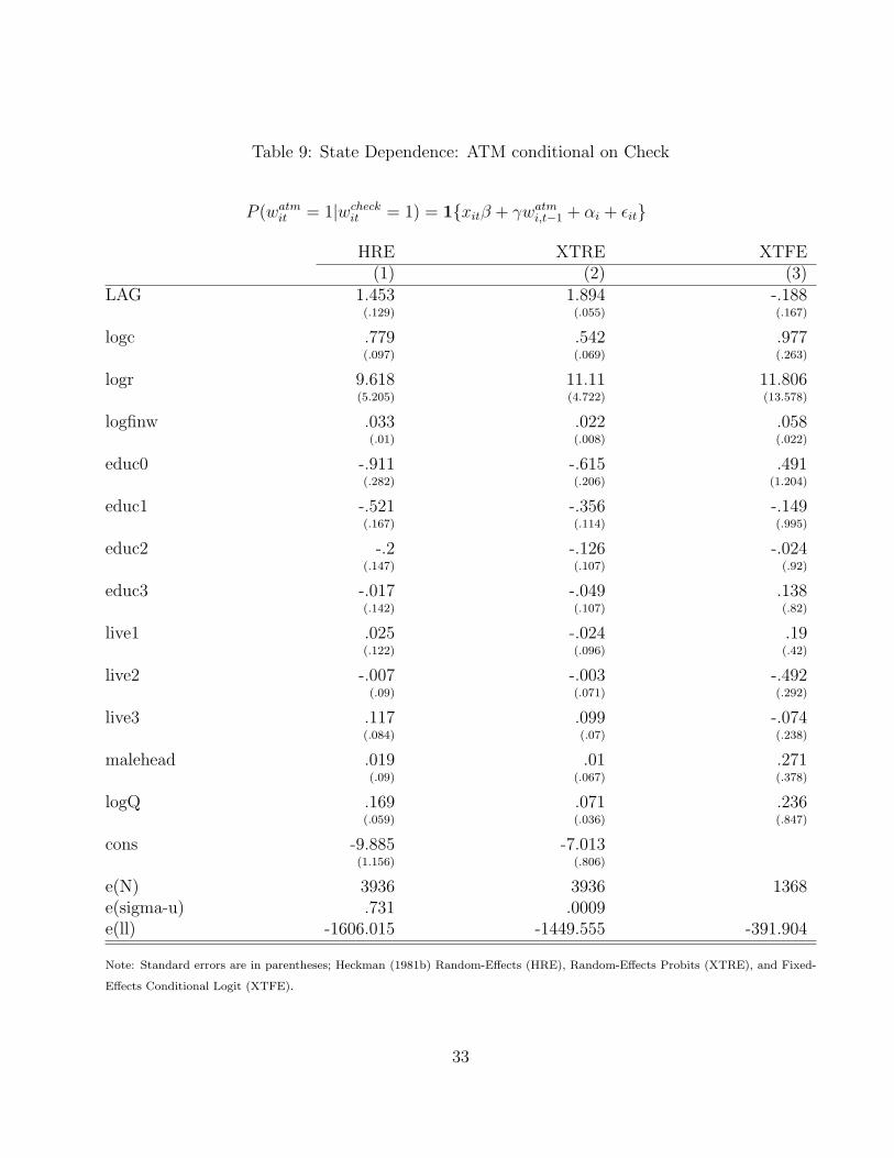
Table 9: State Dependence: ATM conditional on Check

P (watmit = 1|wcheck

it = 1) = 1{xitβ + γwatmi,t−1 + αi + εit}


LAG 1.453 1.894 -.188(.129) (.055) (.167)

logc .779 .542 .977(.097) (.069) (.263)

logr 9.618 11.11 11.806(5.205) (4.722) (13.578)

logfinw .033 .022 .058(.01) (.008) (.022)

educ0 -.911 -.615 .491(.282) (.206) (1.204)

educ1 -.521 -.356 -.149(.167) (.114) (.995)

educ2 -.2 -.126 -.024(.147) (.107) (.92)

educ3 -.017 -.049 .138(.142) (.107) (.82)

live1 .025 -.024 .19(.122) (.096) (.42)

live2 -.007 -.003 -.492(.09) (.071) (.292)

live3 .117 .099 -.074(.084) (.07) (.238)

malehead .019 .01 .271(.09) (.067) (.378)

logQ .169 .071 .236(.059) (.036) (.847)

cons -9.885 -7.013(1.156) (.806)

e(N) 3936 3936 1368e(sigma-u) .731 .0009e(ll) -1606.015 -1449.555 -391.904



33

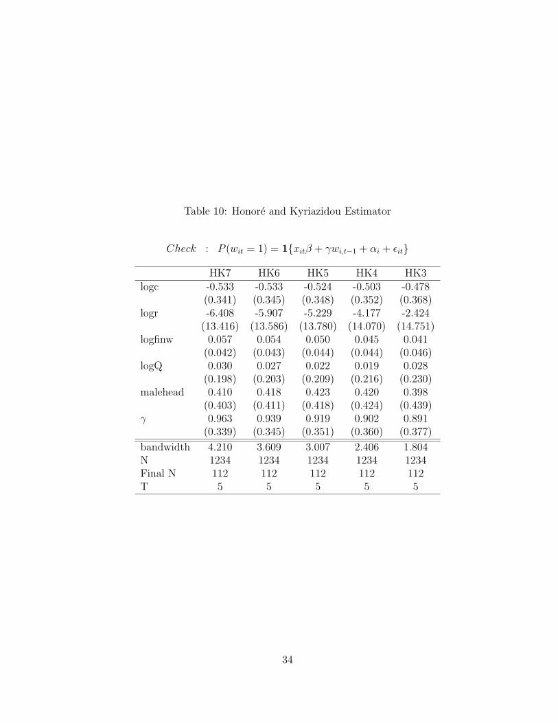
Table 10: Honore and Kyriazidou Estimator

Check : P (wit = 1) = 1{xitβ + γwi,t−1 + αi + εit}

HK7 HK6 HK5 HK4 HK3logc -0.533 -0.533 -0.524 -0.503 -0.478

(0.341) (0.345) (0.348) (0.352) (0.368)logr -6.408 -5.907 -5.229 -4.177 -2.424

(13.416) (13.586) (13.780) (14.070) (14.751)logfinw 0.057 0.054 0.050 0.045 0.041

(0.042) (0.043) (0.044) (0.044) (0.046)logQ 0.030 0.027 0.022 0.019 0.028

(0.198) (0.203) (0.209) (0.216) (0.230)malehead 0.410 0.418 0.423 0.420 0.398

(0.403) (0.411) (0.418) (0.424) (0.439)γ 0.963 0.939 0.919 0.902 0.891

(0.339) (0.345) (0.351) (0.360) (0.377)

bandwidth 4.210 3.609 3.007 2.406 1.804N 1234 1234 1234 1234 1234Final N 112 112 112 112 112T 5 5 5 5 5

34


ATM : P (wit = 1) = 1{xitβ + γwi,t−1 + αi + εit}

HK7 HK6 HK5 HK4 HK3logc 0.529 0.501 0.475 0.446 0.412

(0.443) (0.453) (0.462) (0.468) (0.472)logr 26.791 28.167 29.055 29.063 27.611

(22.315) (22.844) (23.365) (23.868) (24.565)logfinw 0.076 0.073 0.069 0.064 0.060

(0.035) (0.035) (0.036) (0.037) (0.037)logQ 8.260 8.377 8.481 8.556 8.559

(3.479) (3.560) (3.644) (3.731) (3.854)malehead -0.003 -0.004 -0.001 0.013 0.051

(0.762) (0.787) (0.808) (0.826) (0.855)γ 2.062 2.065 2.070 2.077 2.086

(0.235) (0.241) (0.247) (0.250) (0.253)bandwidth 4.210 3.609 3.007 2.406 1.804N 1234 1234 1234 1234 1234Final N 300 300 300 300 300T 5 5 5 5 5

35


CATM : P (watmit = 1|wcheck

it = 1) = 1{xitβ + γwatmi,t−1 + αi + εit}

HK7 HK6 HK5 HK4 HK3logc 0.801 0.783 0.764 0.742 0.714

(0.477) (0.484) (0.490) (0.494) (0.497)logr 21.723 23.246 24.237 24.369 23.111

(23.837) (24.233) (24.595) (24.979) (25.671)logfinw 0.041 0.040 0.037 0.034 0.029

(0.040) (0.040) (0.041) (0.042) (0.043)logQ 6.966 7.059 7.132 7.165 7.109

(3.590) (3.640) (3.691) (3.752) (3.862)malehead -0.537 -0.541 -0.541 -0.532 -0.506

(0.667) (0.683) (0.696) (0.710) (0.732)γ 2.039 2.038 2.039 2.043 2.050

(0.250) (0.254) (0.257) (0.258) (0.260)bandwidth 4.279 3.667 3.056 2.445 1.834N 984 984 984 984 984Final N 257 257 257 257 257T 5 5 5 5 5

36

the decision to use alternative payment methods, state...

Documents