December 2016 Department for Communities and Local Government

The DCLG Appraisal Guide

© Crown copyright, 2016

Copyright in the typographical arrangement rests with the Crown.

You may re-use this information (not including logos) free of charge in any format or medium, under the terms of the Open Government Licence. To view this licence,http://www.nationalarchives.gov.uk/doc/open-government-licence/version/3/ or write to the Information Policy Team, The National Archives, Kew, London TW9 4DU, or email: psi@nationalarchives.gsi.gov.uk.

This document/publication is also available on our website at www.gov.uk/dclg

If you have any enquiries regarding this document/publication, complete the form at http://forms.communities.gov.uk/ or write to us at:

Department for Communities and Local Government Fry Building 2 Marsham Street London SW1P 4DF Telephone: 030 3444 0000

For all our latest news and updates follow us on Twitter: https://twitter.com/CommunitiesUK

December 2016

ISBN: 978-1-4098-4831-8

Contents

ACKNOWLEDGEMENTS 5

FOREWORD 6

LIST OF ABBREVIATIONS 7

DCLG APPRAISAL GROUP 8

INTRODUCTION 9

SECTION 1: THE STRATEGIC CASE 12

SECTION 2: ASSESSING VALUE FOR MONEY 14

APPRAISAL SUMMARY TABLE (AST) 14 BENEFIT COST RATIO (BCR) 16 EMPLOYMENT 22 EXTERNALITIES 23 IMPACT ASSESSMENT METRICS 25 MULTI-CRITERIA ANALYSIS 25 NON-MONETISED IMPACTS 26 PUBLIC SERVICE TRANSFORMATION, SOCIAL POLICIES & FISCAL BENEFITS 26 SPATIAL LEVEL OF ANALYSIS 27 UNITS OF ACCOUNT 28 VALUE FOR MONEY CATEGORIES 28

SECTION 3: LAND VALUE UPLIFT APPROACH TO APPRAISING DEVELOPMENT 31

WHAT IS LAND VALUE UPLIFT? 31 ACCOUNTING FOR EXTERNAL IMPACTS 33 USING LAND VALUE UPLIFT IN COST BENEFIT ANALYSIS 33 ESTIMATING THE GROSS IMPACT OF AN INTERVENTION 35 ESTIMATING THE NET IMPACT OF AN INTERVENTION 36 DISTRIBUTIONAL CONSIDERATIONS 38 OTHER ISSUES TO CONSIDER 39

SECTION 4: ASSUMPTIONS LIST 40

ADDITIONALITY – QUANTITATIVE GUIDANCE 40 ADMINISTRATIVE COSTS OF REGULATION 46 DISTRIBUTIONAL WEIGHTS 47 EMPLOYMENT 47 EXTERNAL IMPACTS OF DEVELOPMENT 47 GDP 48 HOUSE PRICE INDEX 48 INDIRECT TAXATION CORRECTION FACTOR 48 INFLATION 49 LAND VALUE UPLIFT 49 LEARNING RATES 49 OPTIMISM BIAS 49

PLANNING APPLICATIONS 50 PRESENT VALUE YEAR 50 PRIVATE SECTOR COST OF CAPITAL 51 REBOUND EFFECTS 51 REGULATORY TRANSITION COSTS 51

SECTION 5: USEFUL SOURCES OF INFORMATION AND VALUES 52

SECTION 6 - ANNEXES 53

ANNEX A – APPRAISAL SUMMARY TABLE EXAMPLE AND TEMPLATE 53 ANNEX B – GVA APPROACH TO APPRAISING DEVELOPMENT 57 ANNEX C – LAND VALUE UPLIFT FOR RESIDENTIAL DEVELOPMENT 59 ANNEX D – LAND VALUE UPLIFT FOR NON-RESIDENTIAL DEVELOPMENT (WHEN LOCAL LAND VALUE DATA IS AVAILABLE) 65 ANNEX E – ESTIMATING VALUE FOR MONEY FOR NON-RESIDENTIAL DEVELOPMENT USING LAND VALUE UPLIFT NUMBERS WHERE AVAILABLE 74 ANNEX F – EXTERNALITIES ASSOCIATED WITH DEVELOPMENT 81 ANNEX G – DISTRIBUTIONAL IMPACTS 92 BIBLIOGRAPHY 96

5

Acknowledgements We would like to thank the following organisations and people for their support and input in the development of this document.

• All Economists at the Department for Communities and Local Government

• Department for Business, Energy and Industrial Strategy

• Department for Transport

• HM Treasury

• The Homes and Communities Agency

• Michael Spackman, NERA

6

Foreword Assessing the value for money of projects and programmes is a critical part of the policy making process, enabling Ministers to make informed decisions based on the potential costs and benefits of different options. However, doing this presents a number of challenges.

Firstly, scarce public resources means there is a need for robust and rigorous appraisal of costs and benefits in order to extract maximum public value for the tax-payer.

Secondly, the public sector is making increasing use of innovative policy solutions and methods of funding rather than relying on traditional grant-based funding assistance and regulation. Today, there is a greater use of financial instruments and alternatives to regulation which pose analytical and appraisal challenges that need to be addressed.

Finally, and most importantly, when it comes to any economic appraisal, sound judgement is critical. There are usually many unknowns that mean impacts are not always monetised and where judgement about how to account for such impacts is needed. This Guide is designed to support those involved in economic appraisal to make these judgements.

Although this Guide has been designed primarily for economists in DCLG as a means of appraising specific developments in the residential and commercial sectors, it also has wider applications and will be of interest to economists in other areas of the public sector.

I am therefore very pleased to recommend the use of this guidance as a means of helping to deliver better evidenced-based policy making and I look forward to future improvements to the Guide that should make it even more helpful.

Stephen Aldridge,

Chief Analyst, Department for Communities and Local Government

7

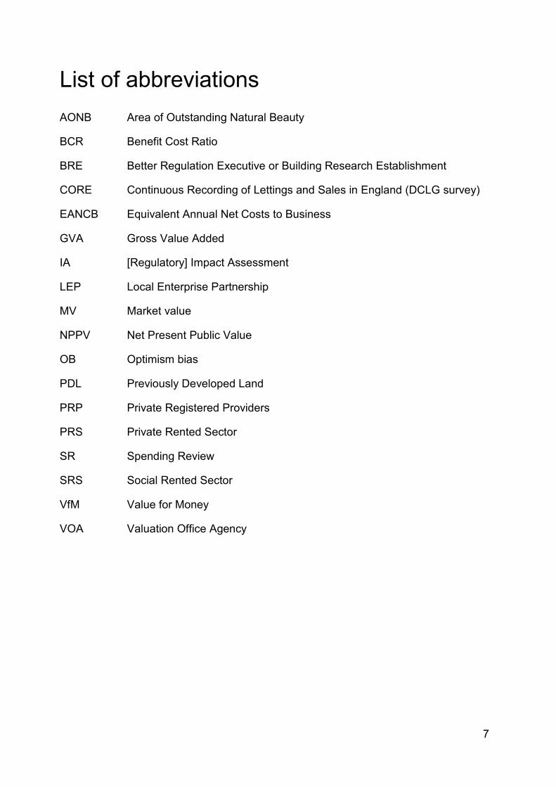
List of abbreviations AONB Area of Outstanding Natural Beauty

BCR Benefit Cost Ratio

BRE Better Regulation Executive or Building Research Establishment

CORE Continuous Recording of Lettings and Sales in England (DCLG survey)

EANCB Equivalent Annual Net Costs to Business

GVA Gross Value Added

IA [Regulatory] Impact Assessment

LEP Local Enterprise Partnership

MV Market value

NPPV Net Present Public Value

OB Optimism bias

PDL Previously Developed Land

PRP Private Registered Providers

PRS Private Rented Sector

SR Spending Review

SRS Social Rented Sector

VfM Value for Money

VOA Valuation Office Agency

8

DCLG Appraisal Group

• Stephen Aldridge, Chief Analyst at the Department for Communities and Local Government

• Matthew Carson, Economic Advisor, Housing and Planning Analysis

• Paul Chamberlain (Chair), Deputy Director of Integration, Decentralisation and Deregulation, Appraisal

• David Craine, Economic Advisor, Housing and Planning Analysis

• Zainab Kizilbash Agha, Senior Policy Advisor (former Economic Advisor), Cities and Local Growth Unit

• Scott Dennison, Deputy Director of Housing and Planning Analysis

• Stephen Smith (lead author and editor), Economic Advisor, Integration, Decentralisation and Deregulation, Appraisal

• Ben Toogood, Senior Economic Advisor, Housing and Planning Analysis

• Cody Xuereb, Economic Advisor, Local Policy Analysis

9

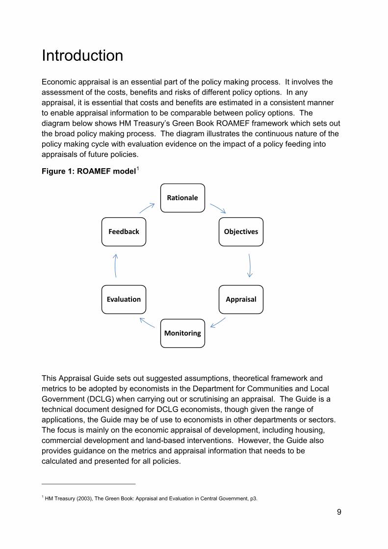
Introduction Economic appraisal is an essential part of the policy making process. It involves the assessment of the costs, benefits and risks of different policy options. In any appraisal, it is essential that costs and benefits are estimated in a consistent manner to enable appraisal information to be comparable between policy options. The diagram below shows HM Treasury’s Green Book ROAMEF framework which sets out the broad policy making process. The diagram illustrates the continuous nature of the policy making cycle with evaluation evidence on the impact of a policy feeding into appraisals of future policies.

Figure 1: ROAMEF model1

This Appraisal Guide sets out suggested assumptions, theoretical framework and metrics to be adopted by economists in the Department for Communities and Local Government (DCLG) when carrying out or scrutinising an appraisal. The Guide is a technical document designed for DCLG economists, though given the range of applications, the Guide may be of use to economists in other departments or sectors. The focus is mainly on the economic appraisal of development, including housing, commercial development and land-based interventions. However, the Guide also provides guidance on the metrics and appraisal information that needs to be calculated and presented for all policies.

1 HM Treasury (2003), The Green Book: Appraisal and Evaluation in Central Government, p3.

Rationale

Objectives

Appraisal

Monitoring

Evaluation

Feedback

10

Some of the key principles from HM Treasury’s Green Book2 are set out in this document with an explanation of how they should be applied in DCLG appraisals. As well as being consistent with the Green Book, this document has been developed in tandem with the current Green Book 'refresh' and is consistent with the Department for Transport’s (DfT) recommended approach to appraising dependent development which is set out in their online appraisal guidance, WebTAG. In addition, while the DCLG Appraisal Guide focuses purely on economic appraisal, ex post evaluations are an important part of the policy making cycle (see ROAMEF model above) and therefore evaluation evidence should be an important component of the evidence base underlying an appraisal.

The assumptions and metrics set out in the Appraisal Guide should be the default when carrying out appraisal for policy development and advice, business cases and Impact Assessments (IAs). However, users are free to adopt different assumptions, frameworks and metrics where appropriate. If users wish to do this, it is essential a clear explanation for doing so is documented in the relevant business case or IA for audit trail purposes.

The Analysis and Data Directorate (ADD) has created this Guide to:

• help ensure consistency in DCLG appraisals;

• help improve the audit trail and justification of certain assumptions; and

• improve the quality of methods and assumptions employed in DCLG appraisals over the long term by improving transparency and understanding and facilitating challenge.

Achieving greater consistency in appraisal will mean the estimated value for money of projects – as measured by the Net Present Public Value (NPPV), Benefit Cost Ratio (BCR) or value for money category – will be more comparable to each other. This will enable decision makers to make more informed choices about the projects they wish to support.

A DCLG Appraisal Group has been formed to oversee the updating of this document and any changes to key assumptions and metrics. This Guide will be regularly updated and so will be a 'living' document containing sections which are likely to change between updates. We will keep all assumptions and metrics under continuous review. We would welcome receiving evidence or analysis on any aspect of this guidance so we can improve the quality of our appraisals. Please send this evidence to ChiefEconomistSign-off@communities.gsi.gov.uk.

2 https://www.gov.uk/government/uploads/system/uploads/attachment_data/file/220541/green_book_complete.pdf

11

The Appraisal Guide is structured as follows:

Section 1 provides a short overview of the Strategic Case;

Section 2 sets out what appraisal information is needed and how it should be presented for all policies;

Section 3 sets out the methodology and theoretical basis for appraising and valuing development, both residential and non-residential, using land value uplift;

Section 4 documents the key assumptions that should be the default in DCLG appraisals;

Section 5 sets out useful source of information;

Section 6 contains a series of Annexes which contain further detail on different aspects of the Guide.

12

Section 1: the Strategic case

1.1 The Strategic Case of a business case – or the relevant sections in an IA - sets out the case for change and the rationale for intervention. It should demonstrate that a spending proposal ‘provides business synergy and strategic fit and is predicated upon a robust and evidence based case for change’.3 The Strategic Case should include the rationale for intervention and ‘a clear definition of outcomes and the potential scope for what is to be achieved’.4 The Economic Case should demonstrate that the spending proposal represents value for money and should include an appraisal of a range of realistic and achievable options.5 Economists should ensure they concern themselves with both the Economic and Strategic Case.6

1.2 The ‘underlying rationale is usually founded either in market failure or where there are clear government distributional objectives that need to be met. Market failure refers to where the market has not and cannot of itself be expected to deliver an efficient outcome’.7 If there is no market failure or equity justification, government intervention may be welfare reducing unless the intervention is correcting an existing ‘government failure’. Economists will therefore want to ensure that the rationale for public sector intervention is clear.

1.3 Establishing the rationale for intervention is important for determining the

appropriate counterfactual against which to assess a policy. The counterfactual should usually be the status quo and be a clear articulation of how things will evolve in the absence of the policy being considered, including continuing trends and development proceeding anyway to a slower timetable. For example, there is no additional economic benefit from government providing support for a development which would have happened anyway (though there may be if the development happens quicker, or is of a better quality than it otherwise would be).

1.4 Once a credible counterfactual has been established, this should be compared

against the ‘do something’ scenario. The ‘do something’ represents a forecast of the outcomes that can be expected with the policy in place. By having a consistent definition of the counterfactual and ‘do something’, key appraisal metrics – Benefit Cost Ratios (BCRs) and Net Present Public Value (NPPV) for example – for different policies can be compared.

3HM Treasury (2013), ‘Public Sector Business Cases’, Green Book Supplementary Guidance on Delivering Public Value from Spending Proposals, p11. 4 Ibid. 5 Ibid, p12. 6 The other elements to a business case are the financial, commercial and management cases though there tends to be less direct involvement from economists on these cases. 7 HM Treasury (2003, p11)

13

1.5 This means only outcomes which are additional to the counterfactual should be assessed (see Additionality section for further details on assessing additionality). For example, if a policy is expected to result in the provision of 1,000 housing units but 500 of these units are expected to be delivered in the status quo, then the benefits of the policy should only be for the 500 additional housing units that would not otherwise be delivered. If 1,000 units are expected to be delivered in the status quo, there are no benefits unless the units are delivered faster or are of a higher quality.8

1.6 The status quo and ‘do something’ are likely to be different because of the

existence of a market failure. For example, a market failure could be preventing a development from happening in the status quo which once addressed could be welfare enhancing. An example of this is in the years immediately following the financial crisis in 2008 when failures in the lending market restricted firms' (particularly small firms) ability to access finance to invest. By government intervening and correcting for this market failure, additional development was able to take place.

1.7 Although there may still be credit constraints in the lending market, users will

need to ensure there is sufficient evidence justifying such a claim as the existence of risk is not in itself a market failure e.g. a firm that is not willing to invest in area X because of the level of risk does not mean there is a market failure requiring government intervention. It may simply reflect the fact that the economic (private) benefits are highly uncertain rather than there being a market failure in the lending market. Credit constraints will not be a form of market failure if the lending market is operating normally.

1.8 Another common rationale for intervention for many DCLG interventions is the

existence of externalities which impose costs (or benefits) on third parties. For example, the existence of a brownfield site which cannot be developed due to the presence of contaminated land but which once developed could provide an amenity benefit to society and improved environmental outcomes. Another example is the existence of an information failure, such as consumers not knowing the standard to which buildings are built. Economists will therefore want to ensure there is sufficient evidence justifying the cited market failure and form the appropriate counterfactual and ‘do something’ scenarios accordingly. As the additionality section explains, a weak market failure could imply relatively high levels of deadweight (and therefore small additionality) so it is crucial this is assessed in significant detail.

8 There will be benefits under such a scenario because future impacts are discounted. This means an intervention which has a net benefit to society and is brought forward will, all else being equal, have a higher social benefit than if the same intervention was delivered later.

14

Section 2: Assessing Value for Money

2.1 This section outlines what metrics should be calculated in a DCLG appraisal and how this appraisal information should be presented.

Appraisal Summary Table (AST)

2.2 An appraisal should provide clear and transparent advice to decision makers on different policy options, taking account of costs, benefits, risks and significant non-monetised impacts. The objective of appraisal should be to provide a consistent comparison of benefits and costs. Presenting such information in summary form with detailed analysis underpinning it is crucial if complex technical information is to be communicated effectively.

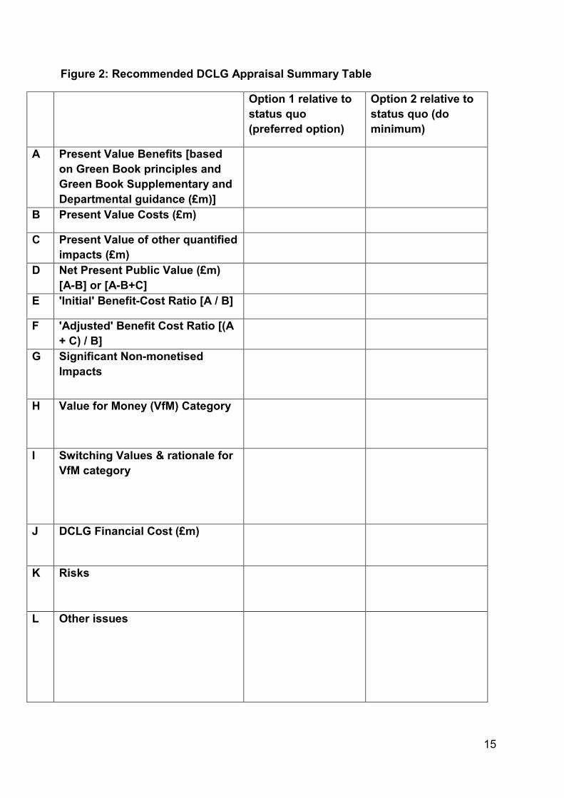
2.3 The table below is a recommended Appraisal Summary Table (AST) which

should be used for all spending proposals. It should feature in business cases and in all documents where appraisal information is contained. The AST aims to capture all the key appraisal information to enable decision makers to understand the value for money of different options. AST's also aim to explain the Benefit Cost Ratio and NPPV in further detail by presenting it in the context of other factors that cannot be reliably monetised and giving an overall judgement on value for money in a value for money category.

2.4 The AST below should be incorporated in all business cases and advice on value

for money of different policy options. Please note this AST is for two policy options. However, a business case should contain several spending options which should be included in an AST. An example of how to complete an AST for a hypothetical scenario is given in Annex A.

15

Figure 2: Recommended DCLG Appraisal Summary Table

Option 1 relative to status quo (preferred option)

Option 2 relative to status quo (do minimum)

A Present Value Benefits [based on Green Book principles and Green Book Supplementary and Departmental guidance (£m)]

B Present Value Costs (£m)

C Present Value of other quantified impacts (£m)

D Net Present Public Value (£m) [A-B] or [A-B+C]

E 'Initial' Benefit-Cost Ratio [A / B]

F 'Adjusted' Benefit Cost Ratio [(A + C) / B]

G Significant Non-monetised Impacts

H Value for Money (VfM) Category

I Switching Values & rationale for VfM category

J DCLG Financial Cost (£m)

K Risks

L Other issues

16

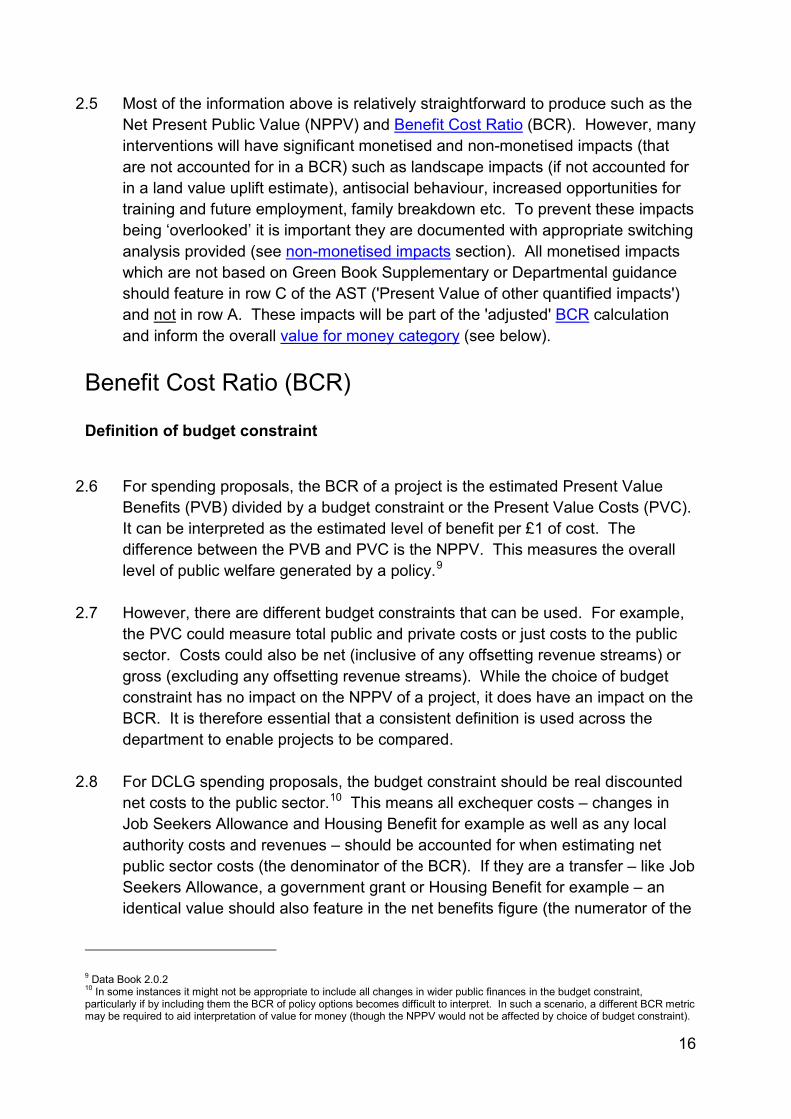
2.5 Most of the information above is relatively straightforward to produce such as the Net Present Public Value (NPPV) and Benefit Cost Ratio (BCR). However, many interventions will have significant monetised and non-monetised impacts (that are not accounted for in a BCR) such as landscape impacts (if not accounted for in a land value uplift estimate), antisocial behaviour, increased opportunities for training and future employment, family breakdown etc. To prevent these impacts being ‘overlooked’ it is important they are documented with appropriate switching analysis provided (see non-monetised impacts section). All monetised impacts which are not based on Green Book Supplementary or Departmental guidance should feature in row C of the AST ('Present Value of other quantified impacts') and not in row A. These impacts will be part of the 'adjusted' BCR calculation and inform the overall value for money category (see below).

Benefit Cost Ratio (BCR) Definition of budget constraint

2.6 For spending proposals, the BCR of a project is the estimated Present Value

Benefits (PVB) divided by a budget constraint or the Present Value Costs (PVC). It can be interpreted as the estimated level of benefit per £1 of cost. The difference between the PVB and PVC is the NPPV. This measures the overall level of public welfare generated by a policy.9

2.7 However, there are different budget constraints that can be used. For example,

the PVC could measure total public and private costs or just costs to the public sector. Costs could also be net (inclusive of any offsetting revenue streams) or gross (excluding any offsetting revenue streams). While the choice of budget constraint has no impact on the NPPV of a project, it does have an impact on the BCR. It is therefore essential that a consistent definition is used across the department to enable projects to be compared.

2.8 For DCLG spending proposals, the budget constraint should be real discounted

net costs to the public sector.10 This means all exchequer costs – changes in Job Seekers Allowance and Housing Benefit for example as well as any local authority costs and revenues – should be accounted for when estimating net public sector costs (the denominator of the BCR). If they are a transfer – like Job Seekers Allowance, a government grant or Housing Benefit for example – an identical value should also feature in the net benefits figure (the numerator of the

9 Data Book 2.0.2 10 In some instances it might not be appropriate to include all changes in wider public finances in the budget constraint, particularly if by including them the BCR of policy options becomes difficult to interpret. In such a scenario, a different BCR metric may be required to aid interpretation of value for money (though the NPPV would not be affected by choice of budget constraint).

17

BCR) unless it is already reflected in a different variable such as land value uplift. Transfers like this have no impact on the NPPV but do impact on the BCR.

2.9 This metric has been selected because: (1) it is a metric that can be used by DCLG, local government and Local Enterprise Partnerships (LEPs) as the budget constraint encompasses all public expenditure and revenues and (2) if projects are prioritised on the basis of the BCR - which impacts on the value for money category - it helps ensure welfare is maximised from a budget closely resembling DCLG’s.

'Initial' and 'Adjusted' BCR for internal business cases and value for money advice

2.10 When estimating the BCR, it is important that there is transparency in what is

included in the benefits and costs. This means being clear about the robustness of the underlying evidence base and the appraisal values being used. It also means being clear when more subjective values are included in the appraisal.

2.11 To account for this, it is recommended two BCRs are calculated: an 'initial' BCR and an 'adjusted' BCR (this is in line with DfT appraisal guidance). The 'initial' BCR takes into account all appraisal values where there is a strong underlying evidence base and which are based on Green Book and Green Book Supplementary and Departmental guidance. A link to a list of this supplementary guidance is given in the footnote below and includes the valuation of the following externalities: air quality, crime, environment, health and greenhouse gas emissions.11 The 'adjusted' BCR may include additional estimates of impacts, based on users’ own evidence i.e. evidence not currently incorporated in Green Book Supplementary and Departmental guidance. These estimates may be based on more tentative assumptions where the evidence base is not so well established (see Annex F). However, both BCRs should inform the overall value for money category of the policy along with appropriate sensitivity analysis.

2.12 For example, suppose there is a market failure in the lending market that is preventing a particular development from taking place. The development is expected to result in an external transport cost of £5m.12 However, there would also be an external benefit from 'cleaning up' the land in the form of an amenity benefit to the surrounding area. There is also expected to be some affordable housing provided as part of the development. These two external impacts - termed 'other quantified impacts' in the AST - are estimated to be in the region of £5m. No other external impacts are expected to result from this proposal.

11 https://www.gov.uk/government/collections/the-green-book-supplementary-guidance 12 Assume this estimate is based on DfT's WebTAG guidance meaning it should feature in the 'initial' BCR.

18

2.13 Assume several policy options are being considered, one of which is a government grant of £10m. With such a grant the development would 'go ahead' and there would be £20m in land value uplift.13 For simplicity assume there is no deadweight or displacement (in practice we would not assume this but the purpose of this example is to demonstrate the calculation of the 'initial' and 'adjusted' BCR). In this example, the present value benefits would be £15m i.e. the £20m land value uplift less the £5m external cost (this cost features in the PVB as it is not a public expenditure cost). The present value costs would be the £10m grant.

2.14 Therefore, in this example, the NPPV would be £5m (the £15m present value

benefits minus the £10m present value costs) and the 'initial' BCR would be 1.5 (the £15m benefits divided by the £10m costs).

2.15 The 'adjusted' BCR would include other quantified impacts. In this instance they

include the benefit from cleaning up the land and the affordable housing, and these are estimated to be £5m. If these appraisal values are included in the analysis, the present value benefits would be equal to £20m (the £15m of benefits in the 'initial' BCR plus the £5m of other quantified impacts) and the economic costs would be £10m. In this case, the NPPV would be £10m (the £20m of benefits minus the £10m of costs) and the 'adjusted' BCR would be 2 (the £20m of economic benefits divided the £10m of economic costs).

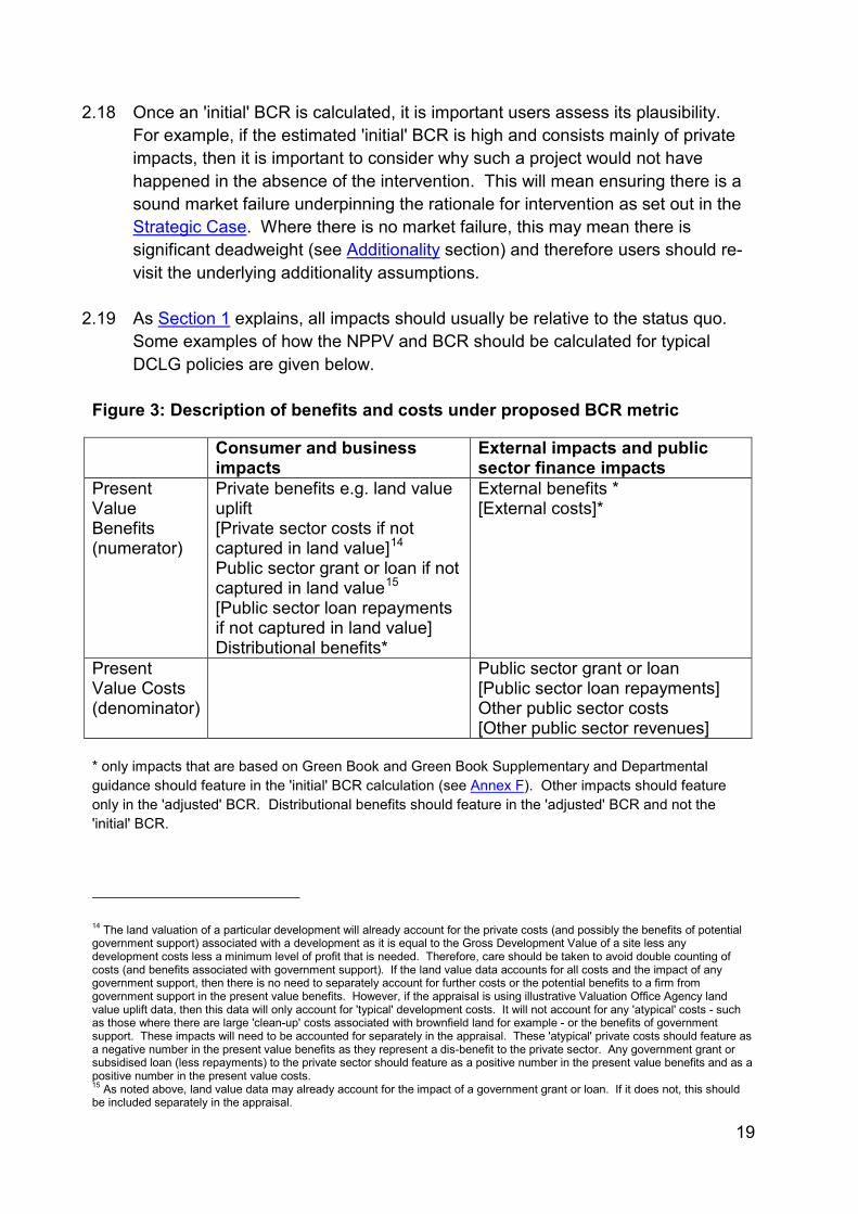
2.16 Figure 3 sets out the types of impacts that would feature in the numerator and

denominator of the BCR for DCLG policies (note those impacts in squared brackets would be negative values). Impacts that should only feature in the 'adjusted' BCR are highlighted. Impacts can be split according to whether they impact on consumers or business (private impacts) or whether they are external or impact on public sector finances (public impacts). Under this metric, no costs to consumers or business feature in the budget constraint (the denominator of the BCR).

2.17 In some instances a BCR may not be appropriate. For example, when there is a

negative or zero cost. For policies such as this – which could include devolution of funding which transfer resources from one place to another – it may be better to focus the value for money analysis on the NPPV and potential Value for Money category.

13 In this example the benefit to the recipient of the £10m grant is reflected in the land value uplift.

19

2.18 Once an 'initial' BCR is calculated, it is important users assess its plausibility. For example, if the estimated 'initial' BCR is high and consists mainly of private impacts, then it is important to consider why such a project would not have happened in the absence of the intervention. This will mean ensuring there is a sound market failure underpinning the rationale for intervention as set out in the Strategic Case. Where there is no market failure, this may mean there is significant deadweight (see Additionality section) and therefore users should re-visit the underlying additionality assumptions.

2.19 As Section 1 explains, all impacts should usually be relative to the status quo.

Some examples of how the NPPV and BCR should be calculated for typical DCLG policies are given below.

Figure 3: Description of benefits and costs under proposed BCR metric

Consumer and business impacts

External impacts and public sector finance impacts

Present Value Benefits (numerator)

Private benefits e.g. land value uplift [Private sector costs if not captured in land value]14 Public sector grant or loan if not captured in land value15 [Public sector loan repayments if not captured in land value] Distributional benefits*

External benefits * [External costs]*

Present Value Costs (denominator)

Public sector grant or loan [Public sector loan repayments] Other public sector costs [Other public sector revenues]

* only impacts that are based on Green Book and Green Book Supplementary and Departmental guidance should feature in the 'initial' BCR calculation (see Annex F). Other impacts should feature only in the 'adjusted' BCR. Distributional benefits should feature in the 'adjusted' BCR and not the 'initial' BCR.

14 The land valuation of a particular development will already account for the private costs (and possibly the benefits of potential government support) associated with a development as it is equal to the Gross Development Value of a site less any development costs less a minimum level of profit that is needed. Therefore, care should be taken to avoid double counting of costs (and benefits associated with government support). If the land value data accounts for all costs and the impact of any government support, then there is no need to separately account for further costs or the potential benefits to a firm from government support in the present value benefits. However, if the appraisal is using illustrative Valuation Office Agency land value uplift data, then this data will only account for 'typical' development costs. It will not account for any 'atypical' costs - such as those where there are large 'clean-up' costs associated with brownfield land for example - or the benefits of government support. These impacts will need to be accounted for separately in the appraisal. These 'atypical' private costs should feature as a negative number in the present value benefits as they represent a dis-benefit to the private sector. Any government grant or subsidised loan (less repayments) to the private sector should feature as a positive number in the present value benefits and as a positive number in the present value costs. 15 As noted above, land value data may already account for the impact of a government grant or loan. If it does not, this should be included separately in the appraisal.

20

2.20 It should be noted that all the impacts in this calculation should be risk adjusted. In the early stages of policy development this will primarily be through Optimism Bias (OB) adjustments to both costs and benefits. Further guidance on OB is given in the Optimism bias section and in the Green Book.

2.21 The examples below set out the calculations for three hypothetical policies to illustrate how the NPPVs and BCRs of DCLG policies are likely to be calculated. For simplicity, assume all figures have been discounted to the appropriate year, are all in real prices and optimism bias has already been applied to both costs and benefits.

Example 1: A DCLG grant to support a development

2.22 One policy option being considered is a £5m grant to support a development on

a brownfield site. The rationale for intervention is the external benefits that may be generated by intervening e.g. improved amenity and health. These external benefits are estimated to be around £5m. However, the development is unlikely to take place in the absence of the intervention because of the high upfront costs of 'cleaning up' the land. These high upfront costs are estimated to be £5m and their existence makes the development commercially unviable i.e. the Gross Development Value does not cover the development costs and a minimum level of profit. Assume that once the land is 'cleaned up' the value of the land in its new use is £5m. Also assume for simplicity that the value of land in its current use is zero and there are no wider external impacts or monetised impacts associated with the intervention other than the improved amenity and health impacts.

2.23 In this example - and for simplicity assuming there is no displacement of economic activity - the 'initial' BCR of intervening would be calculated as follows: the present value benefit is the land value in its new use (£5m) minus the value of the land in its previous use (£0m).16 The estimated cost is the £5m grant. In other words, the NPPV would be £0m and the 'initial' BCR would be 1. However, the other quantified impacts are estimated to be around £5m. By including these impacts in the appraisal, the estimated benefits become £10m and the estimated costs are £5m. This means the NPPV is £5m and the 'adjusted' BCR is 2.0.

16 In this example, for simplicity the £5m benefit to the firm from the grant is not shown given it is financing the private 'clean-up' costs of £5m and so these two terms cancel out.

21

Example 2: A DCLG loan to support brownfield land clean-up and development

2.24 DCLG is approached for a loan to support the redevelopment of a brownfield

site. The rationale for intervention is that there is evidence of market failure in the lending market which is restricting firms access to finance. The development is expected to provide an external amenity and health benefit.

2.25 The site is suitable for 1,000 houses but the high upfront 'clean-up' costs and difficulties in accessing financing make the development commercially unviable. The land value in its new use is £85m based on a financing arrangement which enables the firm to borrow £100m and repay £50m over the appraisal period.17 Once developed, there are potential net external benefits of £10m. Assume for simplicity the value of the site in its current use £10m.

2.26 Assume for simplicity that there is no deadweight or displacement from intervening. In this case, by DCLG providing a loan of £100m and receiving £50m back over the appraisal period, the present value benefits would be equal to the land value in its new use (£85m) less the value of the land its current use (£10m). The present value costs would be the initial loan of £100m less expected repayments of £50m (i.e. £50m net exchequer costs). In this example, the NPPV would therefore be £25m (£75m economic benefits less £50m economic costs). The 'initial' BCR would therefore be 1.5 (£75m economic benefits divided by £50m economic costs).

2.27 When including the potential external benefits of £10m, the present value

benefits increase to £85m while the economic costs are £50m. The NPPV would therefore be £35m and the 'adjusted' BCR would be equal to 1.7.

Example 3: A DCLG grant to subsidise housing for lower income groups

2.28 DCLG pays a grant of £100m to subsidise affordable housing for lower income

groups. The policy is forecast to deliver £100m in land value uplift as a result of the additional housing created. There are also estimated to be £50m worth of distributional benefits and net external benefits associated with this policy.

2.29 In this example, the payment of the grant enables those on lower income groups to live in sub-market rent accommodation. Therefore, while the £100m grant represents a cost to the exchequer, it is also a benefit to the tenants who are now able to live in sub-market accommodation i.e. it is a transfer payment.

17 This means the land value uplift reflects the private benefit of the initial loan and the costs of the subsequent repayments.

22

2.30 In this example, the present value benefits are therefore the £100m land value uplift created plus the £100m benefit to the tenants who are now able to pay sub-market rents. The present value cost is the £100m grant. This means the NPPV is £100m (the £200m economic benefits less the £100m grant) and the 'initial' BCR is 2 (£200m economic benefits divided by £100m grant).

2.31 When including distributional and net external benefits, the economic benefits increase to £250m while the economic costs are £100m. This means the NPPV is £150m and the 'adjusted' BCR is 2.5.

Employment

2.32 The default assumption is that any jobs created by a development resulting from government expenditure do not increase aggregate employment as these employment effects are already largely determined by macroeconomic decisions on the level of overall public expenditure (though they often have an important local impact). As a result, it is recommended that DCLG appraisals do not put a monetary value on these employment impacts unless there is strong evidence of a supply side effect (there is separate work planned on developing external productivity impacts of increased employment density). This approach is consistent with HM Treasury's Green Book.

2.33 In the past, DCLG has used the estimated direct employment and GVA impacts as a measure of the potential benefits of a development (this is explained in Annex B). However, the department’s preferred approach to appraising a development is to use changes in land values to infer the net private impact (see Section 3) and to separately account for external impacts.

2.34 Users are free to quote the number of gross jobs created by a development in

the appraisal. However, these should not be monetised but instead included ‘below the line’ within the appraisal and set out in the Strategic Case. In certain circumstances, users may wish to quote particular metrics – such as those relating to employment or housing – but these should only be in addition to the key value for money metrics (BCR and NPPV) and not instead. These can be included in the AST in the ‘Other issues’ box.

23

Externalities

2.35 An economic appraisal should seek to capture all the benefits and costs associated with an intervention. This will include both private and external impacts. For many DCLG interventions, land value uplift will capture the net private impacts of a development. However, external impacts also need to be captured and can be fundamental to the case for intervention (see Figure 4 and Figure 6).

2.36 All impacts quantified on the basis of Green Book guidance and Green Book Supplementary and Departmental guidance should feature in the 'initial' BCR calculation. These impacts currently include:

• Air quality • Crime • Private Finance Initiatives • Environmental • Transport (see WebTAG

guidance)

• Public Service Transformation • Asset valuation • Competition • Energy use and greenhouse

gas emissions

2.37 Land value uplift and the amenity cost of development are part of DCLG's

appraisal guidance and therefore should feature in the 'initial' BCR. Additional estimates, for any externalities which are not included in the Green Book and Green Book Supplementary and Departmental guidance, can be included in the 'adjusted' BCR. The department recognises the limits of the current guidance and the difficulties of valuing externalities, particularly as the presence of externalities and their value are likely to vary across different types of investment and location. Current guidance should be seen as a starting point for the calculation of an ‘initial’ BCR, whilst the ‘adjusted’ BCR provides flexibility to introduce new estimates, in place or in addition to those in the current guidance. Users are expected to provide justification and evidence to support estimates.

2.38 The current version of the DCLG Appraisal Guide provides estimates for the external amenity cost of development and the health benefits of additional affordable housing. As mentioned above, the amenity cost of development should feature in the 'initial' BCR. However, the health benefits of additional affordable housing should feature in the 'adjusted' BCR as it is not fully established. However, users can replace these estimates with their own estimates if they have more suitable and robust evidence. Estimates from the Unit Cost Database - explained in the Public Service Transformation, Social Policies & Fiscal Benefits section - is Green Book Supplementary guidance so should be included in the 'initial' BCR.

24

2.39 The DCLG Appraisal Guide is a 'living' document and will be regularly updated. We will continue to review and develop the evidence base on externalities and would welcome views and potential evidence that could help with this.

2.40 As the evidence base evolves, we would expect to see more external impacts

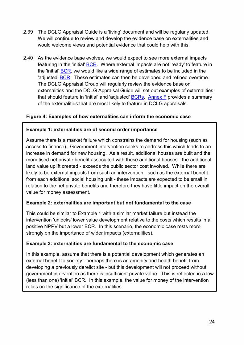
featuring in the 'initial' BCR. Where external impacts are not 'ready' to feature in the 'initial' BCR, we would like a wide range of estimates to be included in the 'adjusted' BCR. These estimates can then be developed and refined overtime. The DCLG Appraisal Group will regularly review the evidence base on externalities and the DCLG Appraisal Guide will set out examples of externalities that should feature in 'initial' and 'adjusted' BCRs. Annex F provides a summary of the externalities that are most likely to feature in DCLG appraisals.

Figure 4: Examples of how externalities can inform the economic case Example 1: externalities are of second order importance

Assume there is a market failure which constrains the demand for housing (such as access to finance). Government intervention seeks to address this which leads to an increase in demand for new housing. As a result, additional houses are built and the monetised net private benefit associated with these additional houses - the additional land value uplift created - exceeds the public sector cost involved. While there are likely to be external impacts from such an intervention - such as the external benefit from each additional social housing unit - these impacts are expected to be small in relation to the net private benefits and therefore they have little impact on the overall value for money assessment.

Example 2: externalities are important but not fundamental to the case

This could be similar to Example 1 with a similar market failure but instead the intervention 'unlocks' lower value development relative to the costs which results in a positive NPPV but a lower BCR. In this scenario, the economic case rests more strongly on the importance of wider impacts (externalities).

Example 3: externalities are fundamental to the economic case

In this example, assume that there is a potential development which generates an external benefit to society - perhaps there is an amenity and health benefit from developing a previously derelict site - but this development will not proceed without government intervention as there is insufficient private value. This is reflected in a low (less than one) 'initial' BCR. In this example, the value for money of the intervention relies on the significance of the externalities.

25

Impact Assessment metrics

2.41 For policies which are likely to have a regulatory impact, an Impact Assessment (IA) is required. An IA aims to set out all the costs and benefits of a proposal, though there is a greater amount of departmental discretion for those policies qualifying for 'fast-track' (see the Better Regulation Executive guidance).

2.42 In an IA, users will be expected to calculate the NPPV of a policy and the Equivalent Annual Net Costs to Business (EANCB). The difference between the two is that the NPPV is an estimate of the impact to society. This includes external impacts such as environmental impacts as well as private impacts to individuals and business. However, the EANCB is focussed purely on the net costs to business. It is defined as the annualised present value of net costs to business and is applicable from the implementation date of the policy.

2.43 As the EANCB is purely an estimate of the impact on business it should exclude

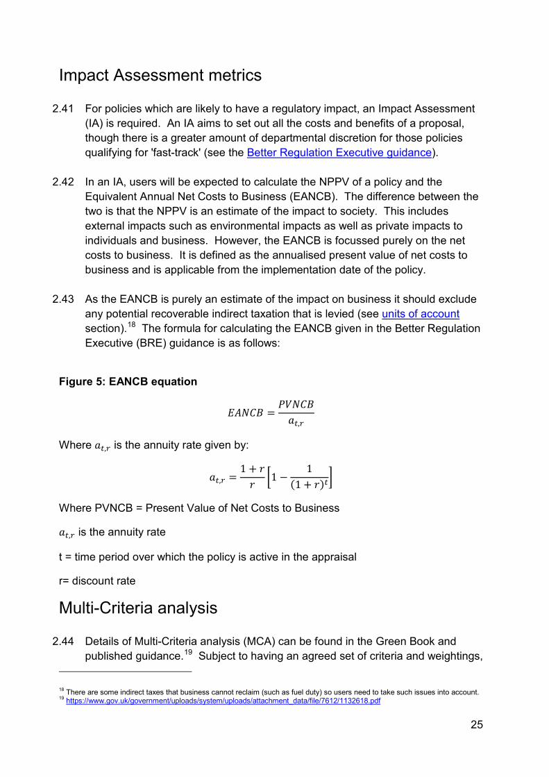
any potential recoverable indirect taxation that is levied (see units of account section).18 The formula for calculating the EANCB given in the Better Regulation Executive (BRE) guidance is as follows:

Figure 5: EANCB equation

𝐸𝐴𝑁𝐶𝐵 =𝑃𝑉𝑁𝐶𝐵𝑎𝑡,𝑟

Where 𝑎𝑡,𝑟 is the annuity rate given by:

𝑎𝑡,𝑟 =1 + 𝑟𝑟

�1 −1

(1 + 𝑟)𝑡�

Where PVNCB = Present Value of Net Costs to Business

𝑎𝑡,𝑟 is the annuity rate

t = time period over which the policy is active in the appraisal

r= discount rate

Multi-Criteria analysis

2.44 Details of Multi-Criteria analysis (MCA) can be found in the Green Book and published guidance.19 Subject to having an agreed set of criteria and weightings,

18 There are some indirect taxes that business cannot reclaim (such as fuel duty) so users need to take such issues into account. 19 https://www.gov.uk/government/uploads/system/uploads/attachment_data/file/7612/1132618.pdf

26

MCA can be a useful ranking tool when there are significant non-monetised impacts. However, MCA does require judgement in establishing objectives and criteria, as well as estimating the relative importance of weights and in judging the contribution of each option to each performance criterion. There is therefore a risk of subjectivity in MCA.

Non-monetised impacts

2.45 There are various ways users may want to deal with non-monetised impacts and it is up to the user to decide how best to handle such impacts. One method is multi criteria analysis (see above) while a further way to capture the significance of such impacts is the use of sensitivity analysis and 'switching values'. A description of switching values is given in the Green Book. The key part to switching analysis involves working backwards and asking the following type of question:

How large do the non-monetised impacts have to be to shift the value for money of the policy from High (where the BCR is greater than 2) to Acceptable (where the BCR is between 1 and 2) or from High to Poor (where the BCR is less than 1)?

2.46 Users will need to state how large – in monetary terms – an impact will have to be to change the overall value for money category. Presenting non-monetised metrics such as output data - number of trees 'lost' as a result of a development or the number of people who visit a particular attraction for example - could help inform decisions on whether such impacts are significant or not (and therefore whether the value for money category needs to change). Users will therefore need to use their judgement in determining the appropriate value for money category.

2.47 It is essential that where monetisation is not possible, a full qualitative

assessment of the potential impacts is carried out. For example, in the context of DCLG appraisals this could include a discussion on the potential environmental and other amenity impacts of changes in land use.

Public Service Transformation, Social Policies & Fiscal Benefits

2.48 In addition to appraising housing related policies, DCLG also leads on appraising

a number of the Government’s major social programmes ranging from the

27

Troubled Families programme, policies to tackle homelessness, rough sleeping, domestic abuse, welfare reform, and policies to encourage public service transformation and integration of services.

2.49 Appraisal of social policies and public service transformation is based on the same principles contained in the Green Book but can present additional challenges. In particular, estimating and monetising the net impact of redesigning services on the use of public services and wider economic and social outcomes. Detailed guidance on appraising public service transformation and social policies is set out in Supporting Public Service Transformation: cost benefit analysis for local partnerships. This document was developed by analysts in DCLG in collaboration, with New Economy Manchester, and the Public Service Transformation Network.

2.50 Alongside this guidance, New Economy Manchester has developed a Unit Cost

Database, to help with the appraisal of service transformation and social policies. Using the best available research from various government and academic sources, the database provides fiscal, economic, and social cost estimates for over 600 outcome measures covering a range of issues from crime, education, employment, fire, health, housing and social services. The database provides costs which can be used to monetise outcomes relevant to social policies in terms of costs to public services (fiscal costs) and the wider economy and society. The database is widely recognised across government as the best available source for information on the costs of a number of issues and is being extensively used for various appraisal projects across government departments and local authorities.

2.51 In addition to the guidance and the Unit Cost Database, New Economy has also

produced a model which acts as a template for carrying out cost benefit analysis.

Spatial level of analysis

2.52 Cost benefit analysis involves calculating two metrics for each policy: the NPPV and Benefit Cost Ratio (BCR). Both of these should be estimated at the national level to give insight into the value for money to the exchequer. This means additionality estimates should be at the national rather than local level.

2.53 However, local impacts should still form an important part of an appraisal and feature in any spatial and distributional analysis. If there are significant local impacts, then this information should be presented alongside the national level appraisal information. For example, in the context of an Impact Assessment, a policy which has significant rural impacts must contain rural proofing analysis within it. Alternatively, a spending proposal which has significant local impacts

28

should be set out within a business case and summarised in the Appraisal Summary Table.

Units of account

2.54 The factor price unit of account excludes indirect taxation while the market price unit of account includes it. As per Green Book guidance, costs and benefits should normally be presented in market prices. This unit of account reflects the best alternative uses that goods and services could be put to (the opportunity cost). The use of market prices means that costs and benefits are generally expressed in units of consumption or consumption equivalent.

Value for money categories

2.55 A Value for Money (VfM) category should be produced for each spending option. A VfM category is an assessment of the overall VfM of a policy based on monetised and non-monetised impacts. As well as providing a more holistic and comprehensive assessment of VfM rather than a narrow BCR approach, VfM categories help ensure greater consistency in the presentation of appraisal information and help avoid the temptation to produce inflated and non-robust BCRs.

2.56 A VfM category will ultimately be a judgement based on the size of the monetised benefits relative to monetised costs (the BCR) and the potential significance of non-monetised impacts. To produce a VfM category, an initial VfM category should be derived based on the 'initial' and 'adjusted' BCR. The value for money categories based on the size of the BCR is given below.

BCR < 1 = Poor value for money

1 ≤ BCR < 2 = Acceptable value for money

BCR ≥ 2 = High value for money

29

2.57 There is a clear rationale for the Poor VfM category as this would mean the policy being considered has costs greater than benefits. However, in practice the BCR should be greater than 1 given the existence of non-monetised factors and given a pound in spending is not identical to a pound in welfare.

2.58 The High VfM category would mean the intervention is expected to deliver twice the amount of benefit per unit of cost hence why it is termed High VfM. Please note if the policy involved is positive NPPV and is zero or negative cost – meaning a BCR cannot be calculated – then the VfM category should be High.

2.59 Where the 'initial' and 'adjusted' BCR result in the same value for money category, then this should be the appropriate value for money category to use before non-monetised impacts are considered. Where the value for money categories differ, a judgement needs to be made about which is most appropriate. It may only be appropriate to determine this after sensitivity analysis and appropriate consideration of non-monetised impacts.

2.60 Users are free to decide the most appropriate way of dealing with non-monetised

impacts e.g. using sensitivity analysis to understand how large these non-monetised impacts need to be to change a value for money category. However, it is essential any approach and subsequent judgement is transparent and clear to decision makers.

2.61 One way to make such a judgement transparent is to carry out sensitivity analysis and highlight key ‘switching values’. In other words, to highlight how large the non-monetised impact has to be to change a value for money category (an example is given below). This analysis could include a 'switching value' on additionality i.e. how big does the additionality need to be to make the policy being appraised Acceptable value for money.

2.62 To make the judgement transparent, value for money categories and BCRs should be communicated in a value for money statement (which should also include the relevant AST). A value for money statement will simply state what the estimated value for money category is and why.

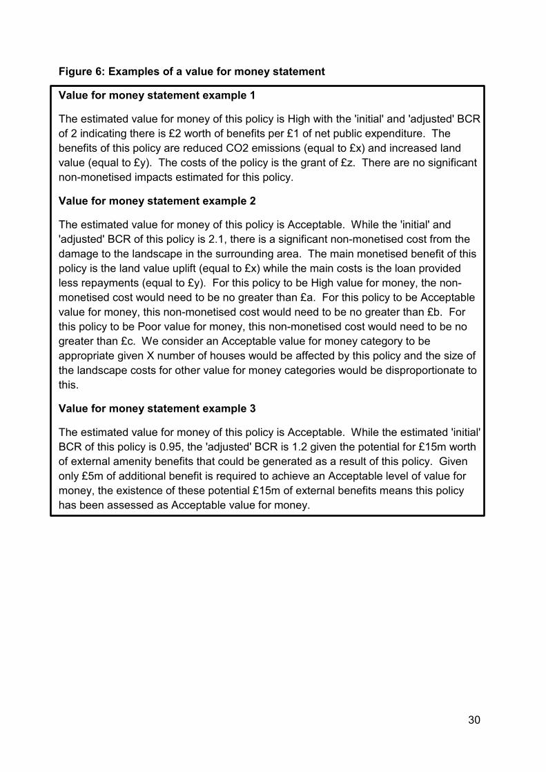
2.63 If the value for money category shifts because of the existence of significant non-monetised impacts then the value for money statement will need to explain this. There is no set way of producing a value for money statement as users will have different approaches for handling non-monetised impacts. Three examples of how judgement has been used to inform a value for money category are set out in the value for money statements below.

30

Figure 6: Examples of a value for money statement

Value for money statement example 1

The estimated value for money of this policy is High with the 'initial' and 'adjusted' BCR of 2 indicating there is £2 worth of benefits per £1 of net public expenditure. The benefits of this policy are reduced CO2 emissions (equal to £x) and increased land value (equal to £y). The costs of the policy is the grant of £z. There are no significant non-monetised impacts estimated for this policy.

Value for money statement example 2

The estimated value for money of this policy is Acceptable. While the 'initial' and 'adjusted' BCR of this policy is 2.1, there is a significant non-monetised cost from the damage to the landscape in the surrounding area. The main monetised benefit of this policy is the land value uplift (equal to £x) while the main costs is the loan provided less repayments (equal to £y). For this policy to be High value for money, the non-monetised cost would need to be no greater than £a. For this policy to be Acceptable value for money, this non-monetised cost would need to be no greater than £b. For this policy to be Poor value for money, this non-monetised cost would need to be no greater than £c. We consider an Acceptable value for money category to be appropriate given X number of houses would be affected by this policy and the size of the landscape costs for other value for money categories would be disproportionate to this.

Value for money statement example 3

The estimated value for money of this policy is Acceptable. While the estimated 'initial' BCR of this policy is 0.95, the 'adjusted' BCR is 1.2 given the potential for £15m worth of external amenity benefits that could be generated as a result of this policy. Given only £5m of additional benefit is required to achieve an Acceptable level of value for money, the existence of these potential £15m of external benefits means this policy has been assessed as Acceptable value for money.

31

Section 3: Land value uplift approach to appraising development

3.1 This section explains DCLG’s recommended and preferred approach to valuing

the benefits of development.20 This approach is also set out in DfT’s WebTAG.21 A step-by-step guide for how to appraise residential development is given in Annex C. For non-residential development, step by step guides are given in Annex D and Annex E.

What is land value uplift?

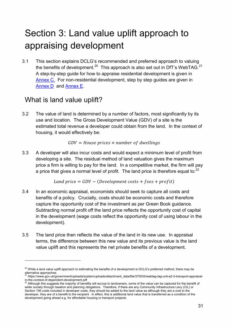
3.2 The value of land is determined by a number of factors, most significantly by its use and location. The Gross Development Value (GDV) of a site is the estimated total revenue a developer could obtain from the land. In the context of housing, it would effectively be:

𝐺𝐷𝑉 = 𝐻𝑜𝑢𝑠𝑒 𝑝𝑟𝑖𝑐𝑒𝑠 × 𝑛𝑢𝑚𝑏𝑒𝑟 𝑜𝑓 𝑑𝑤𝑒𝑙𝑙𝑖𝑛𝑔𝑠

3.3 A developer will also incur costs and would expect a minimum level of profit from developing a site. The residual method of land valuation gives the maximum price a firm is willing to pay for the land. In a competitive market, the firm will pay a price that gives a normal level of profit. The land price is therefore equal to:22

𝐿𝑎𝑛𝑑 𝑝𝑟𝑖𝑐𝑒 = 𝐺𝐷𝑉 − (𝐷𝑒𝑣𝑒𝑙𝑜𝑝𝑚𝑒𝑛𝑡 𝑐𝑜𝑠𝑡𝑠 + 𝑓𝑒𝑒𝑠 + 𝑝𝑟𝑜𝑓𝑖𝑡)

3.4 In an economic appraisal, economists should seek to capture all costs and benefits of a policy. Crucially, costs should be economic costs and therefore capture the opportunity cost of the investment as per Green Book guidance. Subtracting normal profit off the land price reflects the opportunity cost of capital in the development (wage costs reflect the opportunity cost of using labour in the development).

3.5 The land price then reflects the value of the land in its new use. In appraisal terms, the difference between this new value and its previous value is the land value uplift and this represents the net private benefits of a development.

20 While a land value uplift approach to estimating the benefits of a development is DCLG’s preferred method, there may be alternative approaches. 21 https://www.gov.uk/government/uploads/system/uploads/attachment_data/file/370534/webtag-tag-unit-a2-3-transport-appraisal-in-the-context-of-dependent-development.pdf 22 Although this suggests the majority of benefits will accrue to landowners, some of the value can be captured for the benefit of wider society through taxation and planning obligations. Therefore, if there are any Community Infrastructure Levy (CIL) or Section 106 costs included in developer costs, they should be added to the land value as although they are a cost to the developer, they are of a benefit to the recipient. In effect, this is additional land value that is transferred as a condition of the development going ahead e.g. for affordable housing or transport projects.

32

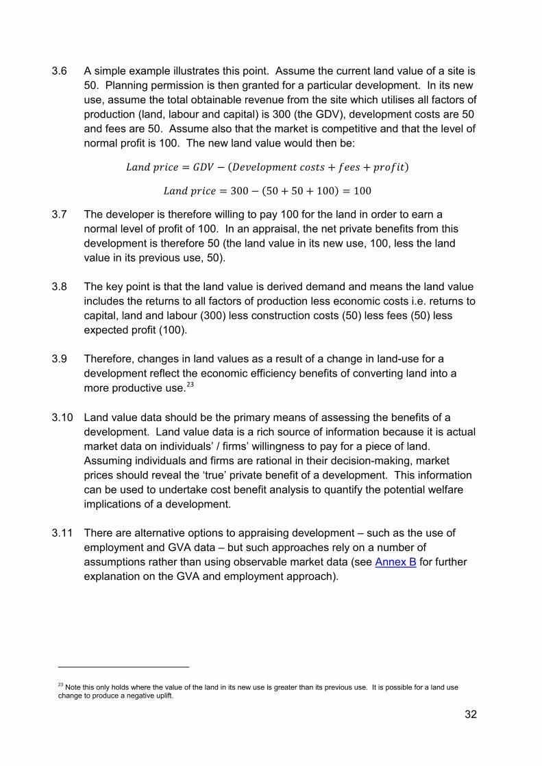
3.6 A simple example illustrates this point. Assume the current land value of a site is 50. Planning permission is then granted for a particular development. In its new use, assume the total obtainable revenue from the site which utilises all factors of production (land, labour and capital) is 300 (the GDV), development costs are 50 and fees are 50. Assume also that the market is competitive and that the level of normal profit is 100. The new land value would then be:

𝐿𝑎𝑛𝑑 𝑝𝑟𝑖𝑐𝑒 = 𝐺𝐷𝑉 − (𝐷𝑒𝑣𝑒𝑙𝑜𝑝𝑚𝑒𝑛𝑡 𝑐𝑜𝑠𝑡𝑠 + 𝑓𝑒𝑒𝑠 + 𝑝𝑟𝑜𝑓𝑖𝑡)

𝐿𝑎𝑛𝑑 𝑝𝑟𝑖𝑐𝑒 = 300 − (50 + 50 + 100) = 100

3.7 The developer is therefore willing to pay 100 for the land in order to earn a normal level of profit of 100. In an appraisal, the net private benefits from this development is therefore 50 (the land value in its new use, 100, less the land value in its previous use, 50).

3.8 The key point is that the land value is derived demand and means the land value includes the returns to all factors of production less economic costs i.e. returns to capital, land and labour (300) less construction costs (50) less fees (50) less expected profit (100).

3.9 Therefore, changes in land values as a result of a change in land-use for a development reflect the economic efficiency benefits of converting land into a more productive use.23

3.10 Land value data should be the primary means of assessing the benefits of a development. Land value data is a rich source of information because it is actual market data on individuals’ / firms’ willingness to pay for a piece of land. Assuming individuals and firms are rational in their decision-making, market prices should reveal the ‘true’ private benefit of a development. This information can be used to undertake cost benefit analysis to quantify the potential welfare implications of a development.

3.11 There are alternative options to appraising development – such as the use of employment and GVA data – but such approaches rely on a number of assumptions rather than using observable market data (see Annex B for further explanation on the GVA and employment approach).

23 Note this only holds where the value of the land in its new use is greater than its previous use. It is possible for a land use change to produce a negative uplift.

33

3.12 Note also that land value uplift is concerned purely with the net private benefits of a development. External impacts should be accounted for separately and summed with the net private impacts to give the net social impact. See below for further details on external impacts.

Accounting for external impacts

3.13 Once the private benefits of a development have been calculated, external impacts should be accounted for. The value to society of a change in use of the land may be separated into: (a) the private benefit associated with the change in land use, as represented by the uplift in land value and (b) the net external impact of the resulting development such as any amenity impacts from changes in landscape. The net social impact is then the summation of these two impacts.

3.14 These external impacts are in addition to the land value uplift. Examples of external impacts include improved health outcomes as a result of reduced overcrowding and reduced external costs from reducing rough sleeping. As explained in the externalities section, when accounting for externalities, the 'initial' BCR should be based on all impacts that can be robustly appraised using Green Book and Green Book Supplementary and Departmental guidance. The 'adjusted' BCR should then include a further range of externalities where the evidence base may not be as well established but which are important to consider in the overall appraisal. Examples of these impacts are given in Annex F. The 'initial' and 'adjusted' BCRs, non-monetised impacts and sensitivity analysis should inform the appropriate value for money category of the policy.

Using land value uplift in cost benefit analysis

3.15 Consider a hypothetical market for commercial floor space (this can either be the freehold or rental market). There is a supply curve S1 and demand curve D1 as per diagram below.24

24 For simplicity we have assumed an inelastic supply curve.

34

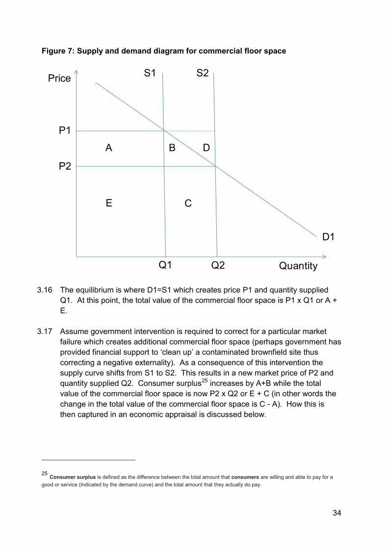
Figure 7: Supply and demand diagram for commercial floor space

3.16 The equilibrium is where D1=S1 which creates price P1 and quantity supplied Q1. At this point, the total value of the commercial floor space is P1 x Q1 or A + E.

3.17 Assume government intervention is required to correct for a particular market failure which creates additional commercial floor space (perhaps government has provided financial support to ‘clean up’ a contaminated brownfield site thus correcting a negative externality). As a consequence of this intervention the supply curve shifts from S1 to S2. This results in a new market price of P2 and quantity supplied Q2. Consumer surplus25 increases by A+B while the total value of the commercial floor space is now P2 x Q2 or E + C (in other words the change in the total value of the commercial floor space is C - A). How this is then captured in an economic appraisal is discussed below.

25 Consumer surplus is defined as the difference between the total amount that consumers are willing and able to pay for a good or service (indicated by the demand curve) and the total amount that they actually do pay.

BA

C

D

P1

P2

Q1 Q2

D1

S1 S2Price

Quantity

E

35

Estimating the gross impact of an intervention

3.18 A new development creates economic value which is reflected in the land value uplift of the land. In this example, area C effectively measures the GDV of the development - the amount of commercial floor space multiplied by the market price - so the land value uplift is equal to area C less development costs less profit less the value of the land in its previous use.

3.19 As well as the land value uplift, there is also a change in the market price from P1 to P2. The reduction in price increases consumer surplus by A + B. However, while A effectively measures the gain to existing tenants of commercial floor space who now pay a lower market price, area A also represents the reduction in the value of existing commercial floor space and is therefore a cost to landlords (see distributional section below).

3.20 Area B represents the consumer surplus gain to 'new' tenants who benefit from

the reduction in the market price for commercial floor space. However, for DCLG appraisals, the gross change in (private) welfare is assumed to equal the value of the development being appraised (area C) less private and public costs, profit and the previous value of the land.26 This value would then reflect the present value of future net private benefits. Area B is therefore effectively ignored as, for a single development, it is likely to be negligible (though this depends on the size of the scheme).27

3.21 In many instances, actual land value data may not be available and therefore illustrative values provided by the department can be used (these are explained in Annex C for residential development and Annex E for non-residential development). However, these values will tend to reflect a price level that is closer to P1 than P2 which means the size of the GDV could be closer to area B + C + D (and therefore accounts for the consumer surplus gain of B). When using such values, the department would expect to see appropriate sensitivity analysis around these values to ensure a robust estimate of the (net) private benefit is made.28

26 As the previous section explains, the residual method of land valuation implies land value uplift equals the final value of the development - the Gross Development Value - less development costs less a minimum level of profit less the value of the land in its current use. 27 If users wish to include an estimate for Area B they need to provide sufficient justification and evidence of the development having a significant impact on the market price (perhaps using local data on rateable commercial floor space). This analysis should also only be undertaken where the policy is marginal e.g. if the BCR is slightly less than 1. Users are free to decide the most effective way of estimating this consumer surplus gain but one way of doing this would be to assume a linear demand curve and estimate the change in welfare as equal to (Q2-Q1)(P1-P2)1/2. 28 This will mean testing whether the policy could have a noticeable impact on land values. Sensitivity analysis is most useful where the policy impacts are non-marginal.

36

Estimating the net impact of an intervention

3.22 As Section 1 and Section 2 explain, all costs and benefits should be relative to a counterfactual. The above example is based on a partial equilibrium analysis in the area where a development takes place. It therefore attempts to estimate the gross impact of an intervention. However, in a general equilibrium context, there are potential impacts that need to be considered in other markets / places. For example, as there will be development in the status quo, we need to account for the possibility that some of the benefits associated with this development would have happened anyway (deadweight) and some benefits that would have occurred no longer do (displacement). Each of these is discussed below.

Estimating deadweight

3.23 Estimating the net impact of a policy requires any impacts which would have

happened anyway to be subtracted from the gross estimates of a policy. In the example above, a critical issue is whether the expansion of commercial floor space (or housing) – and crucially the land value created – would have happened without government intervention, either in the location where the intervention takes place or somewhere else in the economy i.e. ‘while an investment may be additional to the area in which it takes place, it may not be to a wider area or to the country as a whole’.29 Therefore, it is important that when appraising an intervention a correct counterfactual is established (see Section 1 and additionality section).

3.24 A key question to ask when trying to establish a counterfactual like the above is: why does the private sector require government support and would the private investment genuinely not happen without it? If there is a genuine market failure that means the development would not otherwise have happened somewhere in the country without government support then there is no deadweight. However, if it would have gone ahead somewhere in the country anyway, then there is no additional value created.

3.25 Without a sound rationale for intervention (e.g. market failure), a high BCR

consisting of mainly private impacts is potentially a sign of significant deadweight i.e. in the absence of the intervention the market would deliver the same outcomes. In this instance, it would be appropriate to revisit the underlying additionality assumptions underlying the BCR calculation.

29 Venables, A., Overman, H., Laird, J. (2014), Transport investment and economic performance: Implications for project appraisal, p45.

37

3.26 In some instances, it may only be appropriate to include the external impact of a development – such as the positive external (amenity) value of redeveloping a previously derelict site – in the additional economic benefits because the development would have gone ahead somewhere in the country but not necessarily on a brownfield site. Strategic considerations will be important in determining this. For example, the clustering of economic activity of a particular sector in a particular area may mean a firm is unlikely to want to locate somewhere else (see Additionality section).

Estimating displacement

3.27 As well as potential deadweight, for some developments economic activity will be

displaced from one location to another. In an appraisal we should seek to capture the gross impact of a development (as measured by the land value uplift), and deduct any reduction in economic activity from elsewhere (as well as any deadweight). This will give us the net change in land value (or overall additionality).

3.28 There are various ways in which displacement can be accounted for such as:

• Estimating the total change in land prices for all areas e.g. using a land-use transport interaction model;

• Using a spatial general-equilibrium model to estimate how an intervention affects the spatial and sectorial distribution of economic activity; or

• Adjusting the land value uplift for areas with new development.

3.29 Users are free to decide which method is most appropriate, though the method and evidence used should be proportionate to the size and context of the scheme.30 The third option effectively means converting the gross increase in land value into a net change (or calculating an ‘additionality factor’). It should be noted, however, that displacement is more relevant to non-residential developments (see below) and details for how this can be accounted for are given in the additionality section.

30 A useful definition of proportionality can be found in WebTAG: https://www.gov.uk/government/uploads/system/uploads/attachment_data/file/427078/webtag-tag-guidance-for-the-technical-project-manager.pdf

38

Distributional considerations

3.30 In the example in Figure 7, there is a reduction in price following the increase in the supply of a good (commercial floor space or additional housing for example). In this market, the reduction in price in response to the increase in supply means a reduction in land value for those who owned commercial floor space (or housing) before the intervention (this reduction is equal to area A). However, this reduction is a transfer to consumers in the form of increased consumer surplus. For example, the economic benefit of expanding office space is captured by ‘companies that use the offices (in the form of rents being lower than they otherwise would have been) or to workers (in the form of higher wages). Income is thus transferred ‘from existing office owners to office users’.31

3.31 In a housing context, the ‘release of new land for development reduces the scarcity of residential land, and so reduces the value of existing residential land. This reduction in value should be regarded as having purely distributional effects – there is a transfer from the asset-rich who lose out from new development, to the asset-poor, including non-home-owners, who gain’.32

3.32 In both these examples, the key point is that the change in land value for existing land owners is a transfer and so should be a distributional consideration in the analysis. However, the additional (gross) land value generated by the new development is not a transfer as the land use has now changed into a more productive use (though note this land value may simply be displaced - see Additionality section for further guidance).

3.33 An important point to note is that there is a difference between residential and non-residential development. Constrained supply and high demand for housing mean additional housing supply is likely to have only a marginal impact on land values in other locations. However, while housing derives its value from the flow of consumption services to the occupant household, non-residential developments derive their value from their use in the production process. In other words, while the change in the land price of these areas is a transfer, the change in economic activity in these locations may not be. For example, new entrants replacing the firms that might have vacated an area to move into a new area supported by a government grant may be less (or more) profitable than the businesses they replace. This is explained in the additionality section.

31 Venables et al (2014, p48) 32 https://www.gov.uk/government/uploads/system/uploads/attachment_data/file/427094/webtag-tag-unit-a2-3-transport-appraisal-in-the-context-of-dependent-development.pdf, p9.

39

Other issues to consider

3.34 Any private costs associated with the development should be included in the appraisal as a dis-benefit and therefore feature in the numerator of the BCR calculation (unless such costs have already been accounted for in the residual land value estimate – see BCR section for further details). All public sector costs should also be included and feature in the denominator of the BCR.

3.35 When carrying out or reviewing an appraisal, it is essential that there is no double counting of impacts. This could be an issue where local land value data is used. Land value data captures the full net private benefit of a change in land value.33 For example, any utility derived from being close to open space may be reflected the value of the land. In the context of non-residential interventions, in theory, the full private (commercial) benefit of a development will be reflected in the land value, though there may be an external impact on others such as through agglomeration impacts (see Annex F).34

33 If using Valuation Office Agency (VOA) figures on land value uplift, these already include the amenity cost of greenfield development. 34 Consideration will also need to be given as to whether changes in land value are due to existence of transfers e.g. the possibility that the land may benefit from tax-breaks. This could cause the value of the land to change but would represent a transfer from the exchequer to landowners. If the land value increases simply due to the existence of a transfer then this will need to be offset by an equal amount as transfers should have no impact on the NPPV.

40

Section 4: Assumptions list

4.1 This section sets out in alphabetical order recommended assumptions to use in a DCLG appraisal. In some instances – such as with additionality and optimism bias – the relevant assumptions should be formed on a case-by-case basis taking into account the guidance below. Users will therefore need to exercise judgement on the precise assumptions to make.

Additionality – quantitative guidance

4.2 Section 3 outlined the methodology for assessing additionality for all forms of development. This section provides guidance on quantifying the size of the additionality.

4.3 Additionality refers to the extent to which an outcome is genuinely additional. The net impact of a policy therefore excludes any deadweight – impacts which would have happened anyway – and ensures any negative impacts – such as reduced economic activity from elsewhere (displacement) and any economic impacts occurring outside the target area35 (leakage) are also accounted for.

4.4 Therefore, in order to estimate the correct level of additionality, it is essential to

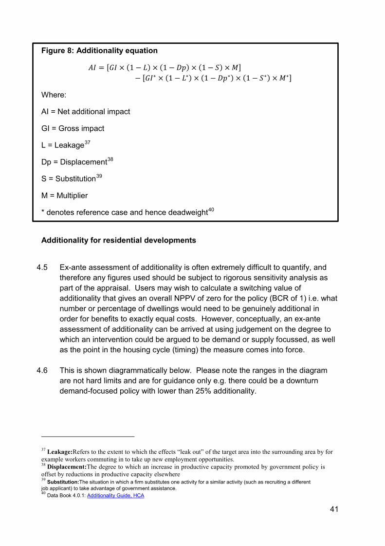
properly determine the counterfactual and work through the logic model of the intervention i.e. clarifying the chain of causation through which inputs translate into outputs and outcomes, both desirable and otherwise. A useful guide to additionality and how users might decide appropriate levels of additionality is the Homes and Communities Agency Additionality Guide (formerly English Partnerships Guide).36 The HCA formula for estimating additionality is:

35 When assessing the overall NPPV and BCR of a policy, the target area is the whole economy so leakage would be with respect to international leakage. However, as part of any distributional analysis, when considering significant spatial impacts, leakage would be with respect to the target area of the policy which would be more local. 36 https://www.gov.uk/government/uploads/system/uploads/attachment_data/file/191511/Additionality_Guide_0.pdf

41

Figure 8: Additionality equation

𝐴𝐼 = [𝐺𝐼 × (1 − 𝐿) × (1 − 𝐷𝑝) × (1 − 𝑆) × 𝑀]− [𝐺𝐼∗ × (1 − 𝐿∗) × (1 −𝐷𝑝∗) × (1 − 𝑆∗) × 𝑀∗]

Where:

AI = Net additional impact

GI = Gross impact

L = Leakage37

Dp = Displacement38

S = Substitution39

M = Multiplier

* denotes reference case and hence deadweight40

Additionality for residential developments

4.5 Ex-ante assessment of additionality is often extremely difficult to quantify, and

therefore any figures used should be subject to rigorous sensitivity analysis as part of the appraisal. Users may wish to calculate a switching value of additionality that gives an overall NPPV of zero for the policy (BCR of 1) i.e. what number or percentage of dwellings would need to be genuinely additional in order for benefits to exactly equal costs. However, conceptually, an ex-ante assessment of additionality can be arrived at using judgement on the degree to which an intervention could be argued to be demand or supply focussed, as well as the point in the housing cycle (timing) the measure comes into force.

4.6 This is shown diagrammatically below. Please note the ranges in the diagram are not hard limits and are for guidance only e.g. there could be a downturn demand-focused policy with lower than 25% additionality.

37 Leakage:Refers to the extent to which the effects “leak out” of the target area into the surrounding area by for example workers commuting in to take up new employment opportunities. 38 Displacement:The degree to which an increase in productive capacity promoted by government policy is offset by reductions in productive capacity elsewhere 39 Substitution:The situation in which a firm substitutes one activity for a similar activity (such as recruiting a different job applicant) to take advantage of government assistance. 40 Data Book 4.0.1: Additionality Guide, HCA

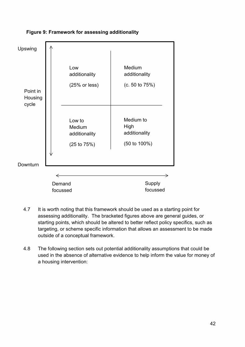
42

Figure 9: Framework for assessing additionality

4.7 It is worth noting that this framework should be used as a starting point for

assessing additionality. The bracketed figures above are general guides, or starting points, which should be altered to better reflect policy specifics, such as targeting, or scheme specific information that allows an assessment to be made outside of a conceptual framework.

4.8 The following section sets out potential additionality assumptions that could be used in the absence of alternative evidence to help inform the value for money of a housing intervention:

Point in Housing cycle

Demand focussed

Supply focussed

Downturn

Upswing

Low to Medium additionality

(25 to 75%)

Medium to High additionality

(50 to 100%)

Low additionality

(25% or less)

Medium additionality

(c. 50 to 75%)

43

4.9 0-25% additionality: policies which fall into this category will be demand focussed and / or about bringing forward housing delivery i.e. the same outcome would have happened in the absence of the intervention but at a later date. The market failure underpinning the intervention may also be less prevalent than in the past (such as access to finance, though we may still expect this to be significant for Small and Medium Enterprises). These policies are therefore likely to have a relatively large amount of deadweight and displacement associated with them.

4.10 25-50% additionality: policies which fall into this category may be demand or

supply focussed but the level of additionality is higher because of the point in the housing cycle when the intervention takes places, and / or because the market failure (ideally supported by local evaluation evidence) is stronger. For example, the policy may be targeted at a particular group like Small and Medium Enterprises (SMEs) or first time buyers. The level of deadweight is therefore likely to be relatively small, though displacement is still likely to be significant.

4.11 50-75% additionality: policies which fall into this category will usually be supply

focussed with good supporting evidence justifying the additionality assumption. Deadweight and displacement are likely to be relatively small. An example would be Affordable Housing where there is strong evidence to suggest housing of this type is unlikely to be built by private developers in the absence of policy and very little crowding out of private development occurs in practice.

4.12 75%+ additionality: policies which fall into this category will usually have a strong supply focus with good supporting evidence. Deadweight and displacement are likely to be small. For example, it could be a policy where there is relatively high ‘clean-up’ costs which mean the site is unviable (and so would not go ahead in the counterfactual) and, like a Garden City, a condition of funding could be that housing would need to be delivered on top of local plans. The site may also be located in an area of high housing need. General economic conditions might also be relatively muted, maximising any additional impacts on the demand side (if applicable).

44

Additionality for non-residential developments

4.13 As Section 3 explains, one way of accounting for potential displacement and

deadweight is to adjust the gross land value uplift estimates of an intervention. To guide users on how this adjustment could be done, the following framework could be used in conjunction with sensitivity analysis in a non-residential appraisal. This framework should be read in conjunction with the market failure and counterfactual discussion in Section 1. Please note, the size of the adjustment factors are purely a guide. If there is evidence on the appropriate size of these adjustment factors then this should be used in the first instance. In the absence of this information, the illustrative figures can be used.

4.14 The framework sets out various criteria that would need to apply for there to be minimal displacement and deadweight from a particular intervention. For example, the existence of a market failure and strong strategic rationale for a development – such as a firm wishing to expand in an area where there is a clustering of industry but is unable to do so because of a market failure in the lending market - and if the industry under consideration has a relatively low level of displacement then we would expect relatively small levels of displacement and deadweight. Therefore, the net impact would be a relatively small adjustment to the gross land value e.g. 75% of the gross land value.

4.15 On the other extreme, where there is a weak market failure and strategic

rationale for intervening, and where the industry under consideration suffers from significant displacement (such as retail), we would adjust the gross land value significantly, with the net impact being 25% or less of the gross land value created.

4.16 Users will need to exercise judgement on the appropriate size of the adjustment

to use taking into account the criteria below. As part of any sensitivity analysis, it may be useful to calculate a 'switching value' i.e. the size of the additionality factor required to make the development NPPV positive.

4.17 The sensitivity analysis on the land value estimate, as well as the potential for

non-monetised impacts and the externalities in Annex F, should inform the value for money category and 'adjusted' BCR. In particular, this sensitivity analysis will be useful in arriving to an overall judgement on the value for money category and whether the value for money category is highly sensitive to adjustments to the gross land value.

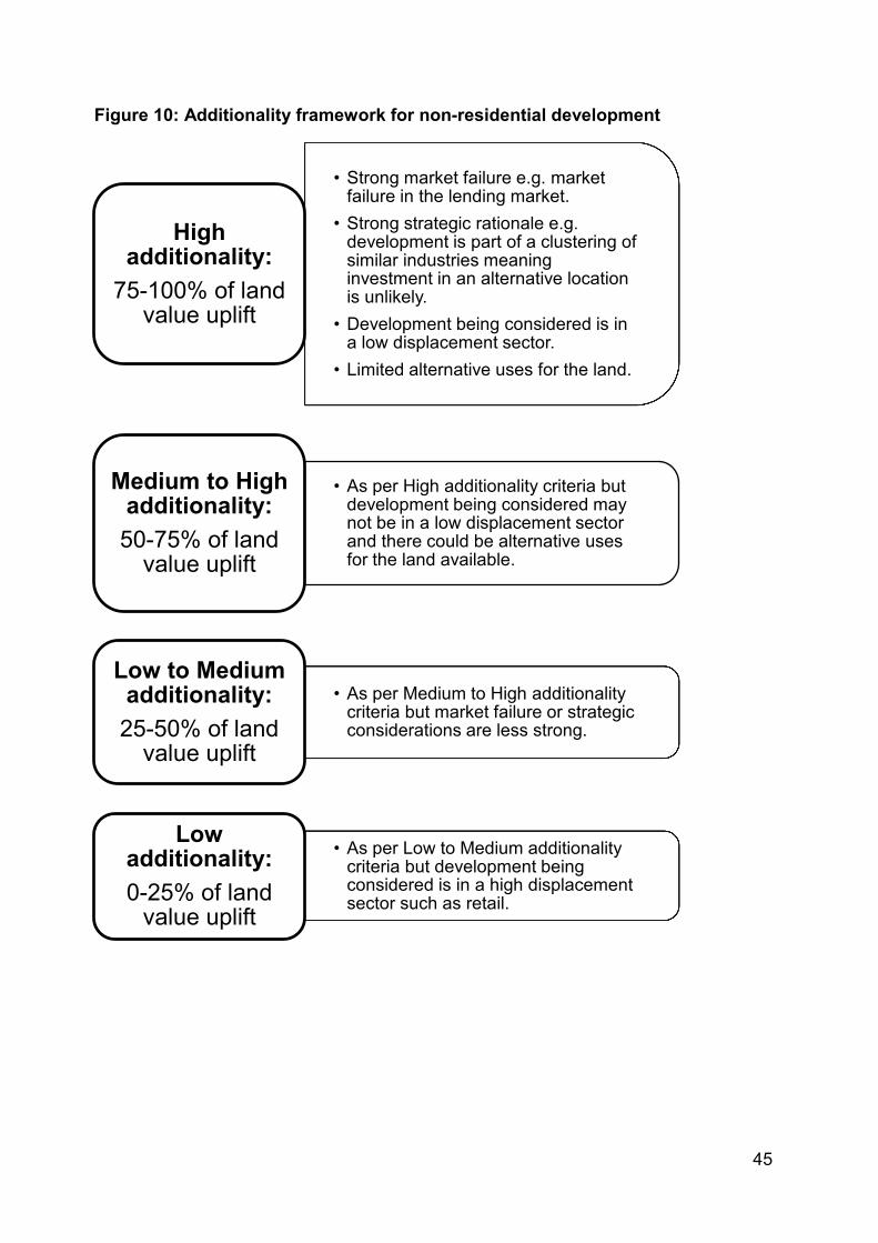
45

Figure 10: Additionality framework for non-residential development

• Strong market failure e.g. market failure in the lending market.

• Strong strategic rationale e.g. development is part of a clustering of similar industries meaning investment in an alternative location is unlikely.

• Development being considered is in a low displacement sector.

• Limited alternative uses for the land.

High additionality:

75-100% of land value uplift

• As per High additionality criteria but development being considered may not be in a low displacement sector and there could be alternative uses for the land available.

Medium to High additionality: 50-75% of land

value uplift

• As per Medium to High additionality criteria but market failure or strategic considerations are less strong.

Low to Medium additionality: 25-50% of land

value uplift

• As per Low to Medium additionality criteria but development being considered is in a high displacement sector such as retail.

Low additionality: 0-25% of land

value uplift

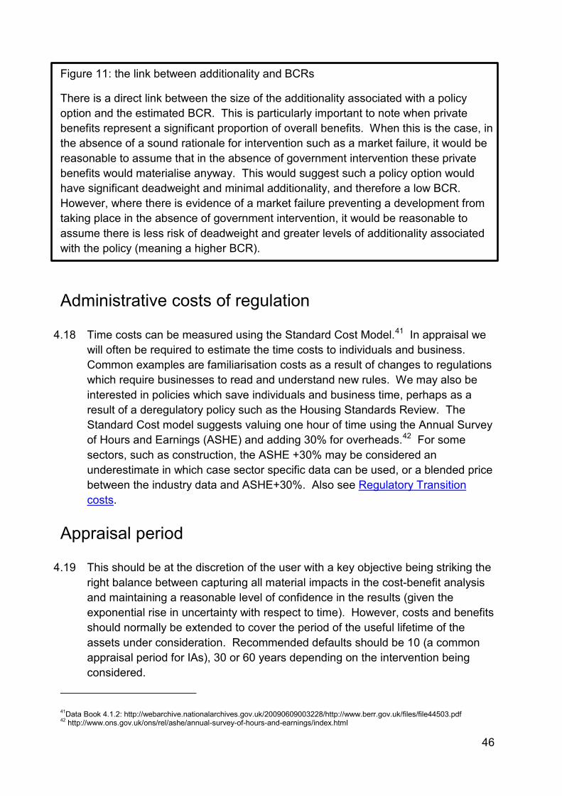
46

Figure 11: the link between additionality and BCRs

There is a direct link between the size of the additionality associated with a policy option and the estimated BCR. This is particularly important to note when private benefits represent a significant proportion of overall benefits. When this is the case, in the absence of a sound rationale for intervention such as a market failure, it would be reasonable to assume that in the absence of government intervention these private benefits would materialise anyway. This would suggest such a policy option would have significant deadweight and minimal additionality, and therefore a low BCR. However, where there is evidence of a market failure preventing a development from taking place in the absence of government intervention, it would be reasonable to assume there is less risk of deadweight and greater levels of additionality associated with the policy (meaning a higher BCR).

Administrative costs of regulation

4.18 Time costs can be measured using the Standard Cost Model.41 In appraisal we will often be required to estimate the time costs to individuals and business. Common examples are familiarisation costs as a result of changes to regulations which require businesses to read and understand new rules. We may also be interested in policies which save individuals and business time, perhaps as a result of a deregulatory policy such as the Housing Standards Review. The Standard Cost model suggests valuing one hour of time using the Annual Survey of Hours and Earnings (ASHE) and adding 30% for overheads.42 For some sectors, such as construction, the ASHE +30% may be considered an underestimate in which case sector specific data can be used, or a blended price between the industry data and ASHE+30%. Also see Regulatory Transition costs.

Appraisal period

4.19 This should be at the discretion of the user with a key objective being striking the right balance between capturing all material impacts in the cost-benefit analysis and maintaining a reasonable level of confidence in the results (given the exponential rise in uncertainty with respect to time). However, costs and benefits should normally be extended to cover the period of the useful lifetime of the assets under consideration. Recommended defaults should be 10 (a common appraisal period for IAs), 30 or 60 years depending on the intervention being considered.

41Data Book 4.1.2: http://webarchive.nationalarchives.gov.uk/20090609003228/http://www.berr.gov.uk/files/file44503.pdf 42 http://www.ons.gov.uk/ons/rel/ashe/annual-survey-of-hours-and-earnings/index.html

47

4.20 Longer appraisal periods are likely to be required for environmental interventions

while shorter appraisal periods may be more relevant to small regulatory changes as per Better Regulation Executive Guide which states that ‘where the appropriate appraisal period is not identifiable, a ten-year period should be used for the analysis.'43 It may also be appropriate to include an allowance for the on-going value of an asset where the appraisal period is truncated.

Distributional weights

4.21 The Green Book provides guidance on the use of distributional weights in cost benefit analysis. The use of distributional weights will be most relevant to policies that have a significant progressive element to them i.e. if the policy benefits low income individuals relatively more than high income individuals. If so, then distributional weights can be used in the calculation of the 'adjusted' BCR but the judgement made on the size of any distributional weights should be made clear for decision makers. Any distributional weighting of impacts should be presented alongside the ‘unadjusted’ cost benefit analysis. See Annex G for an example of how distributional weights have been applied in housing.

Employment

4.22 See employment section for recommended approach.

External impacts of development

4.23 Land value uplift aims to capture the net private benefit associated with a development. However, there are external impacts not accounted for in the land value uplift which should be considered in an appraisal. Some external impacts have well established methodologies - for example valuing carbon emissions - but others, particularly those specific to development, require further work so they can be operationalised into an economic appraisal. A selection of these external impacts is given Annex F. However, all external impacts should be considered in an appraisal and form part of the value for money assessment.

43 https://www.gov.uk/government/uploads/system/uploads/attachment_data/file/421078/bis-13-1038-Better-regulation-framework-manual.pdf, p67.

48

GDP

4.24 If the appraisal involves using future GDP levels or requires the uprating of a variable in line with GDP, the default data to use should be the Office of Budget Responsibility’s latest GDP forecast. This can be found on the OBRs website.44

House price index

4.25 The Office for Budget Responsibility (OBR) produces a forecast of the mix-adjusted house price index (based on the existing Office for National Statistics indices) at a national level. These are published as part of OBR’s Economic and Fiscal Outlook, and can be found in their supplementary economy tables.45 If necessary, future prices beyond the forecast period should be assumed to be in line with long term nominal income growth, consistent with OBR’s forecasting methodology. The current long term nominal income growth is 4%. House price assumptions need to be internally consistent with assumptions made on house building rates. In some instances it may be appropriate to deviate and co-vary both sets of assumptions in sensitivity analysis.

4.26 Depending on the spatial distribution of the policy, it may not be appropriate to use national assumptions for house prices – especially if calculating future returns on investments through e.g. financial instruments in the near term. Users may wish to consider housing cycles at a sub-national level to convey divergences in house price growth at different spatial scales, within the bounds of the national forecast. However, price growth should be assumed to converge towards the long term growth rate of income, as before.

Indirect taxation correction factor

4.27 The indirect taxation correction factor is used to convert between market prices and factor prices. The latest estimate is published by the Department for Transport on WebTAG. This can be found by clicking here.

44 Data Book 4.2.1 http://budgetresponsibility.org.uk/publications/ 45 See: http://budgetresponsibility.org.uk/efo/economic-fiscal-outlook-march-2016/

49

Inflation

4.28 The default should be the GDP deflator. This can be found on the HM Treasury website or by clicking here. For future years not covered by the GDP deflator the Bank of England inflation target (currently 2%) should be used.

Land value uplift

4.29 For quantitative assumptions see Annex C, Annex D and Annex E.

Learning rates

4.30 Where particular prices are expected to increase at significantly higher or lower rates than general inflation, the relative price change should be calculated and factored into the economic appraisals.

4.31 Cost and performance of different technologies can change over time as manufacturers and installers develop processes and technologies that improve performance and reduce costs through experience. For instance if the size of the market for a particular good or service increases, then there is a greater potential for economies of scale, and relative prices may then also be expected to reduce.

4.32 An evidenced estimate for appropriate learning rates for such technologies

should be applied. An example is a ‘Solar PV cost update’ published by the Department of Business, Energy and Industrial Strategy.46

Optimism bias

4.33 Optimism bias (OB) is the systematic tendency for forecasts to underestimate costs and overestimate benefits. Costs and benefits need to be adjusted for OB to gauge the robustness of the value for money of a project. As the Green Book makes clear, the precise level of OB will vary according to the level of uncertainty (for example if you are at the early stages of designing a policy) and the quality of the data and research in the area.47

46 https://www.gov.uk/government/uploads/system/uploads/attachment_data/file/43083/5381-solar-pv-cost-update.pdf (see paragraph 4.1.2). Also see Green Deal IA: https://www.gov.uk/government/uploads/system/uploads/attachment_data/file/42984/5533-final-stage-impact-assessment-for-the-green-deal-a.pdf 47 Data Book 4.3.2 and 4.3.3

50

4.34 Optimism bias should be used to inform decision makers about the risks of costs being higher and benefits being lower than forecast. It is therefore a useful concept in assessing the robustness of a project’s overall value for money. All value for money metrics – the NPPV and BCR – should be calculated with OB included. However, in the financial case of a spending proposal, the OB adjustment should be excluded and instead a reasonable level of contingency should be made (which will be linked to the final level of OB applied in the appraisal at Final Business Case stage - which should ideally be around 2% as per Green Book business case guidance).

4.35 In terms of the level of OB to apply to costs, these should be based on the Green

Book supplementary guidance on OB. Alternatively, if there is more recent and local evidence on appropriate OB to apply, then these should be used.

4.36 There are a number of difficulties with applying OB to estimated benefits and users are free to decide the most appropriate way of accounting for the risk that the estimated benefits will not materialise. In the context of land value uplift, this includes recognising that some of the land value will not be realised due to atypical costs and inefficient firms. However, it should be recognised that when local land value data is used, these risks may, to a large extent, already be accounted for in the private valuation of the land.

Planning applications

4.37 Analysis of the relationship between the number of planning applications and real GDP growth suggests there is a cyclical relationship between the two. Ten year average growth rates (excluding an obvious anomaly in the planning application series in 2008/09) show a close to one-to-one relationship and our provisional modelling of this relationship also suggests a similar relationship. In light of this we recommend the assumption of a one-to-one relationship between real GDP growth and the number of planning applications.

Present Value year

4.38 All future impacts should be discounted back to a common year in order to calculate their present value. The discount rate should be Green Book consistent. The recommended default should be to discount impacts back to the earliest of the following: year in which the first public investment is made, year in which the project opens or year in which the policy takes effect. 48 For EANCB

48 Data Book 4.4.1

51

estimates please consult the BRE guidance for the relevant year (and price base) to discount to.

Private sector cost of capital

4.39 The estimated cost of capital will depend on prevailing market conditions and sector under consideration, e.g. varying with the financing structure (debt / equity mix) of the firms and the riskiness of the business activity. In the absence of alternative data, a typical cost of capital of 10% can be used, though sensitivity analysis around this (7-15%) should be undertaken.

Rebound effects

4.40 Policies which improve energy efficiency may result in energy consumers choosing to use some of their financial savings to buy more energy, for instance for improved comfort. This is known as the ‘rebound effect’. Guidance on valuing direct rebound effects can be found in supplementary green book guidance on ‘Valuation of energy use and greenhouse gas (GHG) emissions’.49

Regulatory transition costs

4.41 Transient, or one-off costs or benefits that occur, which normally relate to the implementation of the measure, should be monetised in addition to on-going policy costs or benefits. One off administrative burdens includes costs associated with familiarisation with administrative requirements, training, record keeping and reporting, including inspection and enforcement of regulation. The Standard Cost model can also be used to estimate these impacts.

49 Para 3.39 onwards in Sept 2014 edition https://www.gov.uk/government/publications/valuation-of-energy-use-and-greenhouse-gas-emissions-for-appraisal

52

Section 5: Useful sources of information and values Better Regulation Executive guidance:

https://www.gov.uk/government/uploads/system/uploads/attachment_data/file/211981/bis-13-1038-better-regulation-framework-manual-guidance-for-officials.pdf

Department for Transport databook:

https://www.gov.uk/government/publications/webtag-tag-data-book-december-2015

English Housing Survey (EHS):

https://www.gov.uk/government/collections/english-housing-survey

Homes and Communities Agency Additionality guidance:

https://www.gov.uk/government/uploads/system/uploads/attachment_data/file/191511/Additionality_Guide_0.pdf

Homes and Communities Agency employment densities guide:

https://www.homesandcommunities.co.uk/sites/default/files/employ-den.pdf

HM Treasury GDP deflator:

https://www.gov.uk/government/collections/gdp-deflators-at-market-prices-and-money-gdp

HM Treasury Green Book and Supplementary and Departmental guidance:

https://www.gov.uk/government/publications/the-green-book-appraisal-and-evaluation-in-central-governent

Office of Budget Responsibility macroeconomic forecasts:

http://budgetresponsibility.org.uk/category/topics/economic-forecasts/

Rural proofing:

https://www.gov.uk/rural-proofing-guidance

BEIS toolkit for valuing carbon emissions:

https://www.gov.uk/government/publications/valuation-of-energy-use-and-greenhouse-gas-emissions-for-appraisal

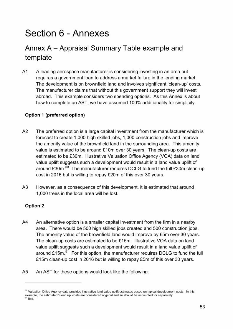
53

Section 6 - Annexes Annex A – Appraisal Summary Table example and template

A1 A leading aerospace manufacturer is considering investing in an area but

requires a government loan to address a market failure in the lending market. The development is on brownfield land and involves significant ‘clean-up’ costs. The manufacturer claims that without this government support they will invest abroad. This example considers two spending options. As this Annex is about how to complete an AST, we have assumed 100% additionality for simplicity.

Option 1 (preferred option)

A2 The preferred option is a large capital investment from the manufacturer which is

forecast to create 1,000 high skilled jobs, 1,000 construction jobs and improve the amenity value of the brownfield land in the surrounding area. This amenity value is estimated to be around £10m over 30 years. The clean-up costs are estimated to be £30m. Illustrative Valuation Office Agency (VOA) data on land value uplift suggests such a development would result in a land value uplift of around £30m.50 The manufacturer requires DCLG to fund the full £30m clean-up cost in 2016 but is willing to repay £20m of this over 30 years.

A3 However, as a consequence of this development, it is estimated that around

1,000 trees in the local area will be lost.

Option 2

A4 An alternative option is a smaller capital investment from the firm in a nearby

area. There would be 500 high skilled jobs created and 500 construction jobs. The amenity value of the brownfield land would improve by £5m over 30 years. The clean-up costs are estimated to be £15m. Illustrative VOA data on land value uplift suggests such a development would result in a land value uplift of around £15m.51 For this option, the manufacturer requires DCLG to fund the full £15m clean-up cost in 2016 but is willing to repay £5m of this over 30 years.

A5 An AST for these options would look like the following:

50 Valuation Office Agency data provides illustrative land value uplift estimates based on typical development costs. In this example, the estimated 'clean up' costs are considered atypical and so should be accounted for separately. 51 Ibid.

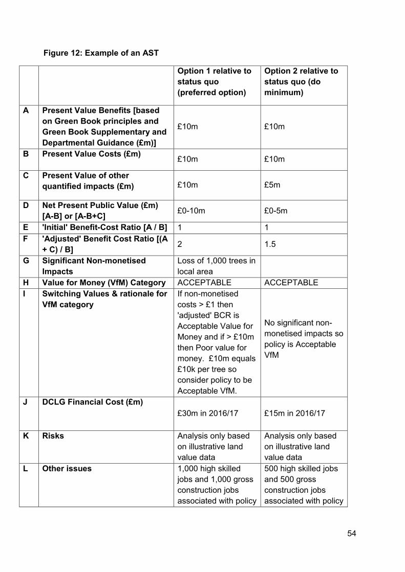
54

Figure 12: Example of an AST

Option 1 relative to status quo (preferred option)

Option 2 relative to status quo (do minimum)

A Present Value Benefits [based on Green Book principles and Green Book Supplementary and Departmental Guidance (£m)]

£10m £10m

B Present Value Costs (£m) £10m £10m

C Present Value of other quantified impacts (£m) £10m £5m

D Net Present Public Value (£m) [A-B] or [A-B+C] £0-10m £0-5m

E 'Initial' Benefit-Cost Ratio [A / B] 1 1 F 'Adjusted' Benefit Cost Ratio [(A

+ C) / B] 2 1.5

G Significant Non-monetised Impacts

Loss of 1,000 trees in local area

H Value for Money (VfM) Category ACCEPTABLE ACCEPTABLE I Switching Values & rationale for

VfM category

If non-monetised costs > £1 then 'adjusted' BCR is Acceptable Value for Money and if > £10m then Poor value for money. £10m equals £10k per tree so consider policy to be Acceptable VfM.

No significant non-monetised impacts so policy is Acceptable VfM

J DCLG Financial Cost (£m) £30m in 2016/17 £15m in 2016/17

K Risks

Analysis only based on illustrative land value data

Analysis only based on illustrative land value data

L Other issues 1,000 high skilled jobs and 1,000 gross construction jobs associated with policy

500 high skilled jobs and 500 gross construction jobs associated with policy

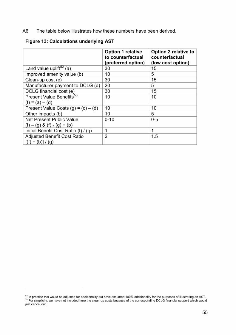
55

A6 The table below illustrates how these numbers have been derived.

Figure 13: Calculations underlying AST

Option 1 relative to counterfactual (preferred option)

Option 2 relative to counterfactual (low cost option)

Land value uplift52 (a) 30 15 Improved amenity value (b) 10 5 Clean-up cost (c) 30 15 Manufacturer payment to DCLG (d) 20 5 DCLG financial cost (e) 30 15 Present Value Benefits53 (f) = (a) – (d)

10 10

Present Value Costs (g) = (c) – (d) 10 10 Other impacts (b) 10 5 Net Present Public Value (f) – (g) & (f) - (g) + (b)

0-10 0-5

Initial Benefit Cost Ratio (f) / (g) 1 1 Adjusted Benefit Cost Ratio [(f) + (b)] / (g)

2 1.5

52 In practice this would be adjusted for additionality but have assumed 100% additionality for the purposes of illustrating an AST. 53 For simplicity, we have not included here the clean-up costs because of the corresponding DCLG financial support which would just cancel out.

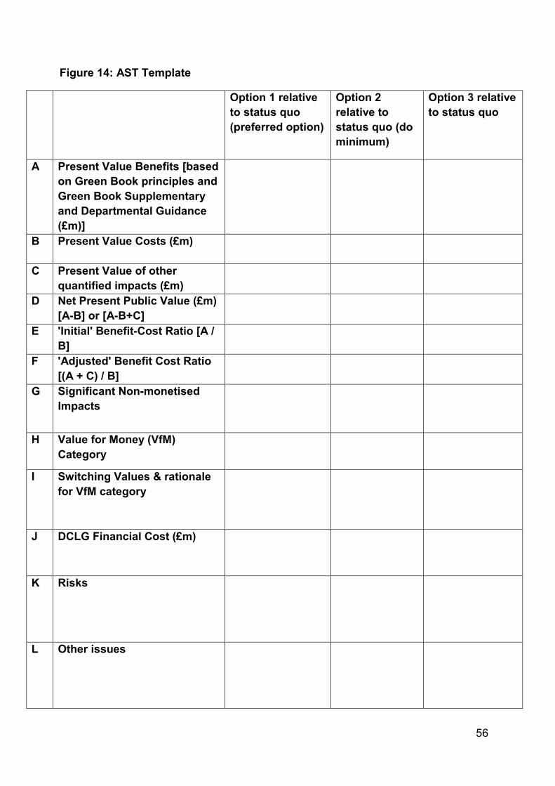
56

Figure 14: AST Template

Option 1 relative to status quo (preferred option)

Option 2 relative to status quo (do minimum)

Option 3 relative to status quo

A Present Value Benefits [based on Green Book principles and Green Book Supplementary and Departmental Guidance (£m)]

B Present Value Costs (£m)

C Present Value of other quantified impacts (£m)

D Net Present Public Value (£m) [A-B] or [A-B+C]

E 'Initial' Benefit-Cost Ratio [A / B]

F 'Adjusted' Benefit Cost Ratio [(A + C) / B]

G Significant Non-monetised Impacts

H Value for Money (VfM) Category

I Switching Values & rationale for VfM category

J DCLG Financial Cost (£m)

K Risks

L Other issues

57

Annex B – GVA approach to appraising development

B1 This annex explains a previously used methodology for appraising non-residential development. This approach is no longer used by the Department and instead changes in land value are used as the primary means of appraising the net private impact of a potential development.

B2 It is important to note that social valuation of a policy or project undertaken to improve land use can be valued in principle either by estimated changes in land values or by estimated changes in the value of the factors that cause the land value to increase (or changes in the economic rent extracted from that land).

B3 In practice, a previous approach to appraising commercial development involved

the following:

• Estimating new commercial floor space: The creation of new commercial floor space was assumed to directly increase economic output by enhancing the capital stock and through raising the productivity of workers. At the time, commercial land value data was considered of insufficient quality to accurately estimate the change in land values following the designation of land for commercial property. Instead, the value of the output of new commercial property was estimated by looking at the additional total value added within new commercial space.

• Estimating new commercial value: To estimate the additional commercial value, the appraisal sought to estimate the additional labour supported by the development. This was calculated using the employment density assumptions and additionality estimates set out in HCA publications (see Section 5). This employment estimate was then combined with Gross Value Added (GVA) data to estimate the net impact of the development. GVA data was used because it was considered more accurate than wages as it also incorporated returns to capital.

B4 Given the GVA of each job was unlikely to be known with precision, regional

GVA data was used to provide an estimate of the annual value of jobs created. These employment outcomes were assumed to build up over a three year period following the creation of the floor space. Assumptions were also made about the persistence of each job (assumed to be 5 years).

B5 Therefore, this approach to valuing non-residential development relied on a number of assumptions, some of which were based on self-reported evaluation evidence. The approach also involved estimating a net employment impact which is now inconsistent with the guidance on monetising employment impacts.

58

B6 While there are drawbacks associated with the land value approach, the DCLG Appraisal Group considers it to be a more suitable and robust approach to appraising the potential private impacts of a development for DCLG policies. It has the unique advantage of being based on observable market data. This estimate can then be built on to include external impacts and other potential impacts.

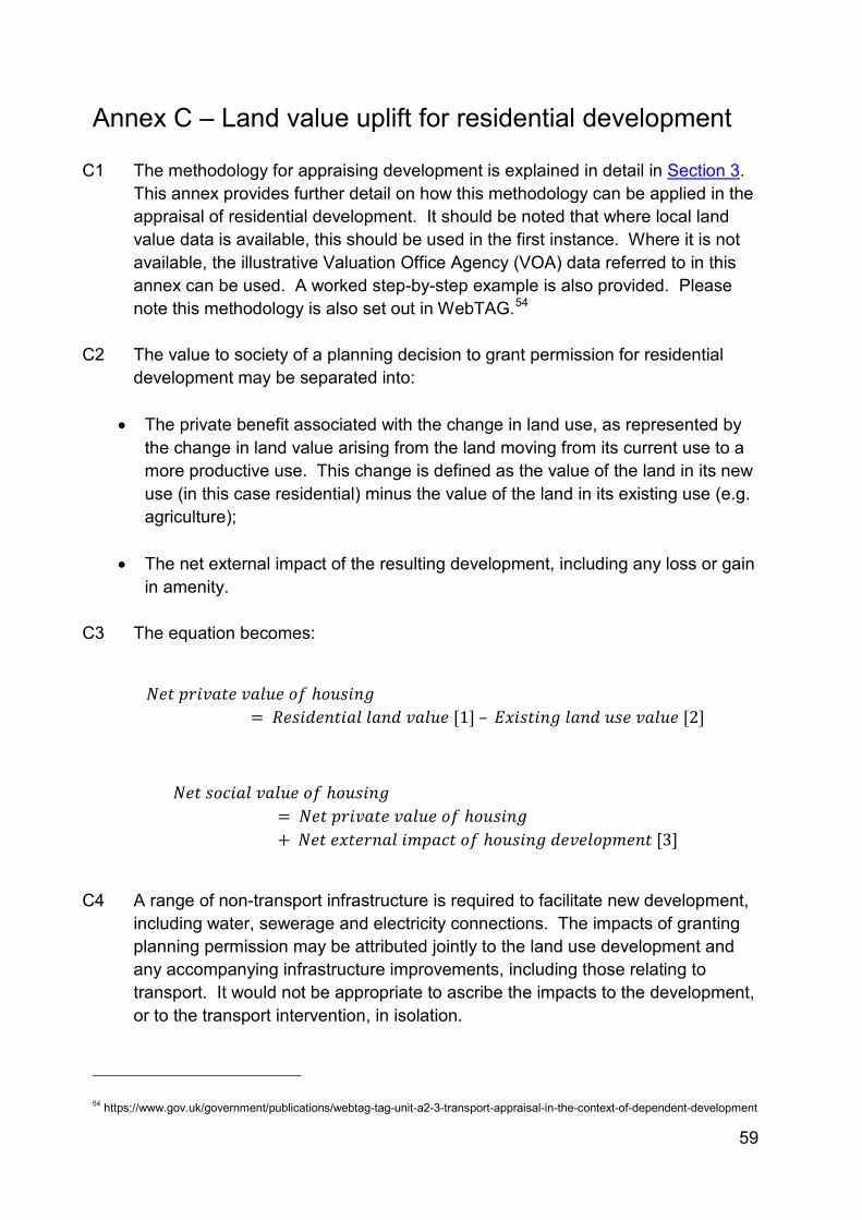
59

Annex C – Land value uplift for residential development

C1 The methodology for appraising development is explained in detail in Section 3. This annex provides further detail on how this methodology can be applied in the appraisal of residential development. It should be noted that where local land value data is available, this should be used in the first instance. Where it is not available, the illustrative Valuation Office Agency (VOA) data referred to in this annex can be used. A worked step-by-step example is also provided. Please note this methodology is also set out in WebTAG.54

C2 The value to society of a planning decision to grant permission for residential development may be separated into:

• The private benefit associated with the change in land use, as represented by

the change in land value arising from the land moving from its current use to a more productive use. This change is defined as the value of the land in its new use (in this case residential) minus the value of the land in its existing use (e.g. agriculture);

• The net external impact of the resulting development, including any loss or gain in amenity.

C3 The equation becomes:

𝑁𝑒𝑡 𝑝𝑟𝑖𝑣𝑎𝑡𝑒 𝑣𝑎𝑙𝑢𝑒 𝑜𝑓 ℎ𝑜𝑢𝑠𝑖𝑛𝑔

= 𝑅𝑒𝑠𝑖𝑑𝑒𝑛𝑡𝑖𝑎𝑙 𝑙𝑎𝑛𝑑 𝑣𝑎𝑙𝑢𝑒 [1] – 𝐸𝑥𝑖𝑠𝑡𝑖𝑛𝑔 𝑙𝑎𝑛𝑑 𝑢𝑠𝑒 𝑣𝑎𝑙𝑢𝑒 [2]

𝑁𝑒𝑡 𝑠𝑜𝑐𝑖𝑎𝑙 𝑣𝑎𝑙𝑢𝑒 𝑜𝑓 ℎ𝑜𝑢𝑠𝑖𝑛𝑔 = 𝑁𝑒𝑡 𝑝𝑟𝑖𝑣𝑎𝑡𝑒 𝑣𝑎𝑙𝑢𝑒 𝑜𝑓 ℎ𝑜𝑢𝑠𝑖𝑛𝑔 + 𝑁𝑒𝑡 𝑒𝑥𝑡𝑒𝑟𝑛𝑎𝑙 𝑖𝑚𝑝𝑎𝑐𝑡 𝑜𝑓 ℎ𝑜𝑢𝑠𝑖𝑛𝑔 𝑑𝑒𝑣𝑒𝑙𝑜𝑝𝑚𝑒𝑛𝑡 [3]

C4 A range of non-transport infrastructure is required to facilitate new development,

including water, sewerage and electricity connections. The impacts of granting planning permission may be attributed jointly to the land use development and any accompanying infrastructure improvements, including those relating to transport. It would not be appropriate to ascribe the impacts to the development, or to the transport intervention, in isolation.

54 https://www.gov.uk/government/publications/webtag-tag-unit-a2-3-transport-appraisal-in-the-context-of-dependent-development

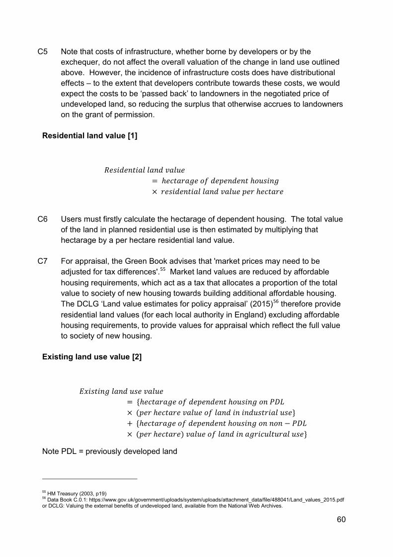
60

C5 Note that costs of infrastructure, whether borne by developers or by the exchequer, do not affect the overall valuation of the change in land use outlined above. However, the incidence of infrastructure costs does have distributional effects – to the extent that developers contribute towards these costs, we would expect the costs to be ‘passed back’ to landowners in the negotiated price of undeveloped land, so reducing the surplus that otherwise accrues to landowners on the grant of permission.

Residential land value [1]

𝑅𝑒𝑠𝑖𝑑𝑒𝑛𝑡𝑖𝑎𝑙 𝑙𝑎𝑛𝑑 𝑣𝑎𝑙𝑢𝑒 = ℎ𝑒𝑐𝑡𝑎𝑟𝑎𝑔𝑒 𝑜𝑓 𝑑𝑒𝑝𝑒𝑛𝑑𝑒𝑛𝑡 ℎ𝑜𝑢𝑠𝑖𝑛𝑔 × 𝑟𝑒𝑠𝑖𝑑𝑒𝑛𝑡𝑖𝑎𝑙 𝑙𝑎𝑛𝑑 𝑣𝑎𝑙𝑢𝑒 𝑝𝑒𝑟 ℎ𝑒𝑐𝑡𝑎𝑟𝑒

C6 Users must firstly calculate the hectarage of dependent housing. The total value

of the land in planned residential use is then estimated by multiplying that hectarage by a per hectare residential land value.

C7 For appraisal, the Green Book advises that 'market prices may need to be adjusted for tax differences'.55 Market land values are reduced by affordable housing requirements, which act as a tax that allocates a proportion of the total value to society of new housing towards building additional affordable housing. The DCLG ‘Land value estimates for policy appraisal’ (2015)56 therefore provide residential land values (for each local authority in England) excluding affordable housing requirements, to provide values for appraisal which reflect the full value to society of new housing.

Existing land use value [2]

𝐸𝑥𝑖𝑠𝑡𝑖𝑛𝑔 𝑙𝑎𝑛𝑑 𝑢𝑠𝑒 𝑣𝑎𝑙𝑢𝑒 = {ℎ𝑒𝑐𝑡𝑎𝑟𝑎𝑔𝑒 𝑜𝑓 𝑑𝑒𝑝𝑒𝑛𝑑𝑒𝑛𝑡 ℎ𝑜𝑢𝑠𝑖𝑛𝑔 𝑜𝑛 𝑃𝐷𝐿 × (𝑝𝑒𝑟 ℎ𝑒𝑐𝑡𝑎𝑟𝑒 𝑣𝑎𝑙𝑢𝑒 𝑜𝑓 𝑙𝑎𝑛𝑑 𝑖𝑛 𝑖𝑛𝑑𝑢𝑠𝑡𝑟𝑖𝑎𝑙 𝑢𝑠𝑒} + {ℎ𝑒𝑐𝑡𝑎𝑟𝑎𝑔𝑒 𝑜𝑓 𝑑𝑒𝑝𝑒𝑛𝑑𝑒𝑛𝑡 ℎ𝑜𝑢𝑠𝑖𝑛𝑔 𝑜𝑛 𝑛𝑜𝑛 − 𝑃𝐷𝐿 × (𝑝𝑒𝑟 ℎ𝑒𝑐𝑡𝑎𝑟𝑒) 𝑣𝑎𝑙𝑢𝑒 𝑜𝑓 𝑙𝑎𝑛𝑑 𝑖𝑛 𝑎𝑔𝑟𝑖𝑐𝑢𝑙𝑡𝑢𝑟𝑎𝑙 𝑢𝑠𝑒}

Note PDL = previously developed land

55 HM Treasury (2003, p19) 56 Data Book C.0.1: https://www.gov.uk/government/uploads/system/uploads/attachment_data/file/488041/Land_values_2015.pdf or DCLG: Valuing the external benefits of undeveloped land, available from the National Web Archives.

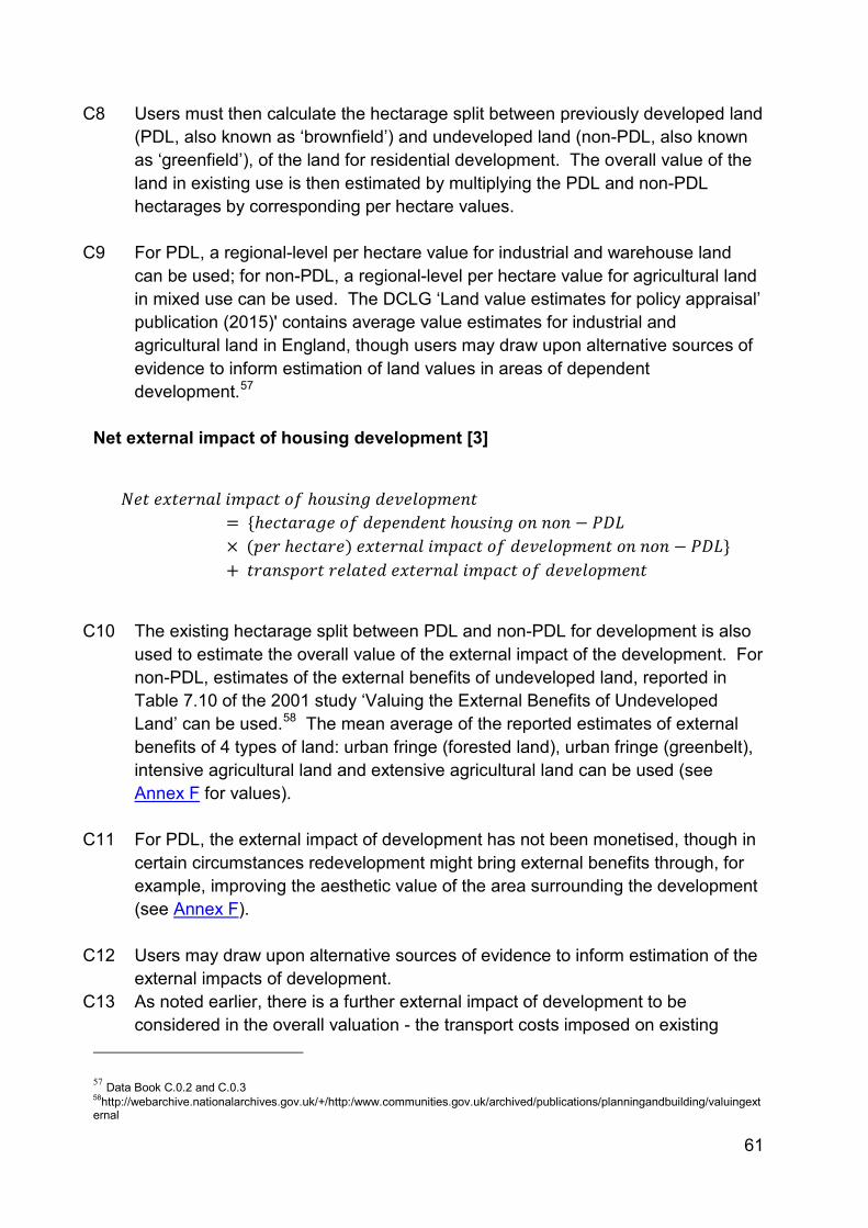
61

C8 Users must then calculate the hectarage split between previously developed land (PDL, also known as ‘brownfield’) and undeveloped land (non-PDL, also known as ‘greenfield’), of the land for residential development. The overall value of the land in existing use is then estimated by multiplying the PDL and non-PDL hectarages by corresponding per hectare values.

C9 For PDL, a regional-level per hectare value for industrial and warehouse land can be used; for non-PDL, a regional-level per hectare value for agricultural land in mixed use can be used. The DCLG ‘Land value estimates for policy appraisal’ publication (2015)' contains average value estimates for industrial and agricultural land in England, though users may draw upon alternative sources of evidence to inform estimation of land values in areas of dependent development.57

Net external impact of housing development [3]

𝑁𝑒𝑡 𝑒𝑥𝑡𝑒𝑟𝑛𝑎𝑙 𝑖𝑚𝑝𝑎𝑐𝑡 𝑜𝑓 ℎ𝑜𝑢𝑠𝑖𝑛𝑔 𝑑𝑒𝑣𝑒𝑙𝑜𝑝𝑚𝑒𝑛𝑡

= {ℎ𝑒𝑐𝑡𝑎𝑟𝑎𝑔𝑒 𝑜𝑓 𝑑𝑒𝑝𝑒𝑛𝑑𝑒𝑛𝑡 ℎ𝑜𝑢𝑠𝑖𝑛𝑔 𝑜𝑛 𝑛𝑜𝑛 − 𝑃𝐷𝐿 × (𝑝𝑒𝑟 ℎ𝑒𝑐𝑡𝑎𝑟𝑒) 𝑒𝑥𝑡𝑒𝑟𝑛𝑎𝑙 𝑖𝑚𝑝𝑎𝑐𝑡 𝑜𝑓 𝑑𝑒𝑣𝑒𝑙𝑜𝑝𝑚𝑒𝑛𝑡 𝑜𝑛 𝑛𝑜𝑛 − 𝑃𝐷𝐿} + 𝑡𝑟𝑎𝑛𝑠𝑝𝑜𝑟𝑡 𝑟𝑒𝑙𝑎𝑡𝑒𝑑 𝑒𝑥𝑡𝑒𝑟𝑛𝑎𝑙 𝑖𝑚𝑝𝑎𝑐𝑡 𝑜𝑓 𝑑𝑒𝑣𝑒𝑙𝑜𝑝𝑚𝑒𝑛𝑡

C10 The existing hectarage split between PDL and non-PDL for development is also

used to estimate the overall value of the external impact of the development. For non-PDL, estimates of the external benefits of undeveloped land, reported in Table 7.10 of the 2001 study ‘Valuing the External Benefits of Undeveloped Land’ can be used.58 The mean average of the reported estimates of external benefits of 4 types of land: urban fringe (forested land), urban fringe (greenbelt), intensive agricultural land and extensive agricultural land can be used (see Annex F for values).

C11 For PDL, the external impact of development has not been monetised, though in certain circumstances redevelopment might bring external benefits through, for example, improving the aesthetic value of the area surrounding the development (see Annex F).

C12 Users may draw upon alternative sources of evidence to inform estimation of the

external impacts of development. C13 As noted earlier, there is a further external impact of development to be

considered in the overall valuation - the transport costs imposed on existing 57 Data Book C.0.2 and C.0.3 58http://webarchive.nationalarchives.gov.uk/+/http:/www.communities.gov.uk/archived/publications/planningandbuilding/valuingexternal

62

users of the network, by residents of the new development. These transport-related external impacts of development should be added to the non-transport-related external impacts discussed above (see Annex F for further details).

C14 For any additional housing that is expected to be delivered in future years, the

values should be uprated by 5% each year in real terms to the relevant year. The 20 year average annual growth in residential land values is 7% (DCLG statistics published to 2010, extended to 2014 using latest unpublished data). The 20 year average growth in the GDP deflator is 2%. Therefore, the average annual real terms growth in residential land values is 5%. To simplify and in the absence of further data, we (conservatively) assume that this applies to all elements of net social land value uplift (i.e. agricultural land values, industrial land values, and externality values).

C15 When carrying out an appraisal of a housing scheme, the starting point should

always be local data. This should include establishing a counterfactual and the number of additional dwellings the policy is then likely to ‘unlock’. An estimate of when each additional dwelling is built and the land value uplift for that year can then be used to estimate the economic benefit of the scheme.

Worked example

C16 A hypothetical residential development delivers five hectares (50,000m2) of

greenfield land for residential use. There is evidence of a market failure in the lending market with developer and local agents unable to secure the financial capital to fund supporting infrastructures for the development (for example roads and waterworks). One policy option being considered is a public sector capital grant of £5m. The developer expects to deliver 40 units per hectare. A ‘Medium’ level of additionality of 50% has been applied to account for deadweight and displacement effects (see Additionality section).

𝑁𝑒𝑡 𝑠𝑜𝑐𝑖𝑎𝑙 𝑣𝑎𝑙𝑢𝑒 𝑜𝑓 ℎ𝑜𝑢𝑠𝑖𝑛𝑔 𝑑𝑒𝑣𝑒𝑙𝑜𝑝𝑚𝑒𝑛𝑡= 𝑁𝑒𝑡 𝑝𝑟𝑖𝑣𝑎𝑡𝑒 𝑣𝑎𝑙𝑢𝑒 𝑜𝑓 ℎ𝑜𝑢𝑠𝑖𝑛𝑔 𝑑𝑒𝑣𝑒𝑙𝑜𝑝𝑚𝑒𝑛𝑡+ 𝑁𝑒𝑡 𝑒𝑥𝑡𝑒𝑟𝑛𝑎𝑙 𝑖𝑚𝑝𝑎𝑐𝑡 𝑜𝑓 ℎ𝑜𝑢𝑠𝑖𝑛𝑔 𝑑𝑒𝑣𝑒𝑙𝑜𝑝𝑚𝑒𝑛𝑡

C17 One hectare of residential land on a typical site in this area is estimated at

around £4.3m59 in 2013-14 prices which is around £108k per unit for this development.

59 Further details on illustrative residential land values can be found at: https://www.gov.uk/government/publications/land-value-estimates-for-policy-appraisal

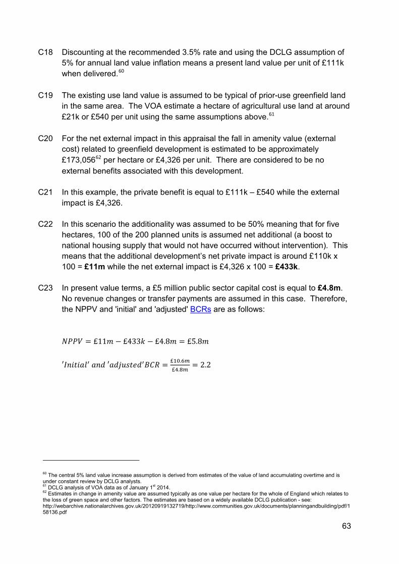
63

C18 Discounting at the recommended 3.5% rate and using the DCLG assumption of 5% for annual land value inflation means a present land value per unit of £111k when delivered.60

C19 The existing use land value is assumed to be typical of prior-use greenfield land in the same area. The VOA estimate a hectare of agricultural use land at around £21k or £540 per unit using the same assumptions above.61

C20 For the net external impact in this appraisal the fall in amenity value (external cost) related to greenfield development is estimated to be approximately £173,05662 per hectare or £4,326 per unit. There are considered to be no external benefits associated with this development.

C21 In this example, the private benefit is equal to £111k – £540 while the external

impact is £4,326.

C22 In this scenario the additionality was assumed to be 50% meaning that for five hectares, 100 of the 200 planned units is assumed net additional (a boost to national housing supply that would not have occurred without intervention). This means that the additional development’s net private impact is around £110k x 100 = £11m while the net external impact is £4,326 x 100 = £433k.

C23 In present value terms, a £5 million public sector capital cost is equal to £4.8m.

No revenue changes or transfer payments are assumed in this case. Therefore, the NPPV and 'initial' and 'adjusted' BCRs are as follows:

𝑁𝑃𝑃𝑉 = £11𝑚 − £433𝑘 − £4.8𝑚 = £5.8𝑚 ′𝐼𝑛𝑖𝑡𝑖𝑎𝑙′ 𝑎𝑛𝑑 ′𝑎𝑑𝑗𝑢𝑠𝑡𝑒𝑑′𝐵𝐶𝑅 = £10.6𝑚

£4.8𝑚= 2.2

60 The central 5% land value increase assumption is derived from estimates of the value of land accumulating overtime and is under constant review by DCLG analysts. 61 DCLG analysis of VOA data as of January 1st 2014. 62 Estimates in change in amenity value are assumed typically as one value per hectare for the whole of England which relates to the loss of green space and other factors. The estimates are based on a widely available DCLG publication - see: http://webarchive.nationalarchives.gov.uk/20120919132719/http://www.communities.gov.uk/documents/planningandbuilding/pdf/158136.pdf

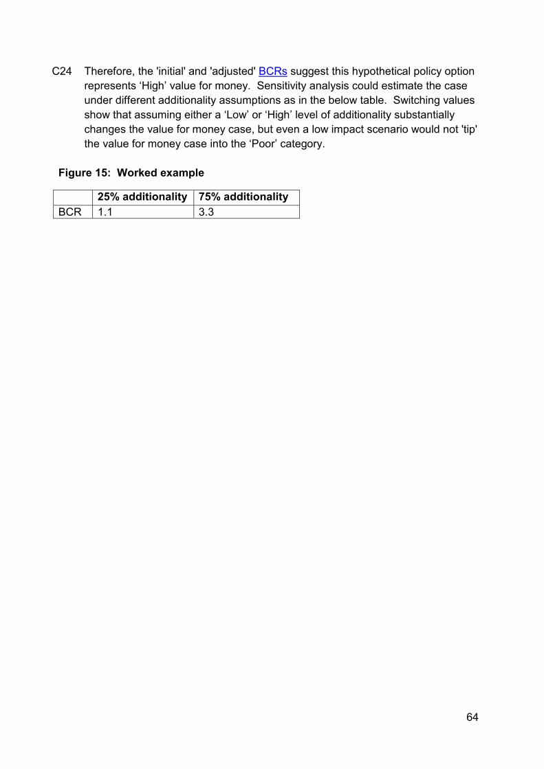
64

C24 Therefore, the 'initial' and 'adjusted' BCRs suggest this hypothetical policy option represents ‘High’ value for money. Sensitivity analysis could estimate the case under different additionality assumptions as in the below table. Switching values show that assuming either a ‘Low’ or ‘High’ level of additionality substantially changes the value for money case, but even a low impact scenario would not 'tip' the value for money case into the ‘Poor’ category.

Figure 15: Worked example

25% additionality 75% additionality BCR 1.1 3.3

65

Annex D – Land value uplift for non-residential development (when local land value data is available)

D1 This note describes DCLG’s preferred approach to valuing the impacts of non-

residential development. The preferred approach involves the use of land value data to assess the private costs and benefits of a policy. In the absence of reliable land value data, Annex E can be followed which provides illustrative VOA land value data. These estimates may also be a useful cross-check to any locally derived land value data.

The approach

D2 The value to society of a planning decision to grant permission for new non-

residential development may be separated into:

• The private benefit associated with the change in land use, as represented by the uplift in land value arising from the land moving from its current use to a more productive use. This uplift is defined as the value of the land in its new use (in this case commercial) minus the value of the land in its existing use (e.g. agriculture);

• The net external impact of the resulting development, including any loss or gain in amenity.

D3 The equation below summarises this:

𝑁𝑒𝑡 𝑝𝑟𝑖𝑣𝑎𝑡𝑒 𝑣𝑎𝑙𝑢𝑒 𝑜𝑓 𝑛𝑜𝑛 − 𝑟𝑒𝑠𝑖𝑑𝑒𝑛𝑡𝑖𝑎𝑙 𝑑𝑒𝑣𝑒𝑙𝑜𝑝𝑚𝑒𝑛𝑡

= 𝐶𝑜𝑚𝑚𝑒𝑟𝑐𝑖𝑎𝑙 𝑙𝑎𝑛𝑑 𝑣𝑎𝑙𝑢𝑒 (1) − 𝐸𝑥𝑖𝑠𝑡𝑖𝑛𝑔 𝑙𝑎𝑛𝑑 𝑢𝑠𝑒 𝑣𝑎𝑙𝑢𝑒 (2)

𝑁𝑒𝑡 𝑠𝑜𝑐𝑖𝑎𝑙 𝑣𝑎𝑙𝑢𝑒 𝑜𝑓 𝑛𝑜𝑛 − 𝑟𝑒𝑠𝑖𝑑𝑒𝑛𝑡𝑖𝑎𝑙 𝑑𝑒𝑣𝑒𝑙𝑜𝑝𝑚𝑒𝑛𝑡= 𝑁𝑒𝑡 𝑝𝑟𝑖𝑣𝑎𝑡𝑒 𝑣𝑎𝑙𝑢𝑒 𝑜𝑓 𝑛𝑜𝑛 − 𝑟𝑒𝑠𝑖𝑑𝑒𝑛𝑡𝑖𝑎𝑙 𝑑𝑒𝑣𝑒𝑙𝑜𝑝𝑚𝑒𝑛𝑡+ 𝑁𝑒𝑡 𝑒𝑥𝑡𝑒𝑟𝑛𝑎𝑙 𝑖𝑚𝑝𝑎𝑐𝑡 𝑜𝑓 𝑛𝑜𝑛 − 𝑟𝑒𝑠𝑖𝑑𝑒𝑛𝑡𝑖𝑎𝑙 𝑑𝑒𝑣𝑒𝑙𝑜𝑝𝑚𝑒𝑛𝑡 (3)

The calculation

D4 Below is a discussion of the key elements of the appraisal, including the data

inputs and underlying assumptions. Note that a number of data inputs must be specified by the user on a case-by-case basis as they relate to the nature of the development in question.

66

Non-residential land value

𝑁𝑜𝑛 − 𝑟𝑒𝑠𝑖𝑑𝑒𝑛𝑡𝑖𝑎𝑙 𝑙𝑎𝑛𝑑 𝑣𝑎𝑙𝑢𝑒 = 𝐻𝑒𝑐𝑡𝑎𝑟𝑎𝑔𝑒 × 𝐿𝑎𝑛𝑑 𝑣𝑎𝑙𝑢𝑒 𝑝𝑒𝑟 ℎ𝑒𝑐𝑡𝑎𝑟𝑒

D5 The total value of the land in planned non-residential use is estimated by multiplying the hectarage of land by a per hectare non-residential land value.

D6 The preference would be to use locally derived land value data to estimate the

land value from post- development. In practice, land values vary substantially on a site-by-site basis, given differences in, for example, proximity to amenities or density of development. As land value estimates are one component of subjective residual valuations made by developers, it is important that an explanation for how these estimates are derived is clearly set out in the economic case and follow the recommendations set out in the Green Book63 for site valuation:

• The valuation of a site should be based on the most valuable possible use,

rather than the highest value that could be obtained for its current use;

• An assessment of the value of a site in the most valuable alternative use should be based on the advice of suitably qualified and experienced valuation surveyor. Either in-house valuers or external experts can be commissioned to carry out the valuation;

• Valuations should be based on the definitions of 'market value' (MV) used in the

'RICS Valuation of Professional Standards’ (the Red Book). Valuations should take into consideration the prospects for development and the presence of any purchaser with a special interest, insofar as the market would do so;

• Site values used should follow the Green Book guidance on prices where

'market prices may need to be adjusted for tax differences'.64 D7 Users are encouraged to draw upon alternative sources of evidence to inform

estimation of land values in areas of dependent development. Where any site values based on recent sales compare sites that are consistent with the intended development on:

63 https://www.gov.uk/government/uploads/system/uploads/attachment_data/file/220541/green_book_complete.pdf 64 HM Treasury (2003, p19)

67

• Business use of site: represent values for sites that have the same business use. Commercial property can be used as an industrial plant, a logistics warehouse, a hi-tech lab or as office space and the value generated by each of these developments is very different.

• State of development of site: represent typical levels of value for sites that are ripe for development, in that they have the following conditions:

o no abnormal site constraints;

o a planning permission of a type generally found in the area;

o services to the edge of the site.

• Measures: used to determine the size of the site should be consistent

Existing land use value [2]

𝐸𝑥𝑖𝑠𝑡𝑖𝑛𝑔 𝑙𝑎𝑛𝑑 𝑢𝑠𝑒 𝑣𝑎𝑙𝑢𝑒 = 𝐻𝑒𝑐𝑡𝑎𝑟𝑎𝑔𝑒 × 𝐿𝑎𝑛𝑑 𝑣𝑎𝑙𝑢𝑒 𝑝𝑒𝑟 ℎ𝑒𝑐𝑡𝑎𝑟𝑒

D8 Again, users may draw upon alternative sources of evidence to inform estimation

of land values.

Net external impact of housing development [3]

𝑁𝑒𝑡 𝑒𝑥𝑡𝑒𝑟𝑛𝑎𝑙 𝑖𝑚𝑝𝑎𝑐𝑡 𝑜𝑓 𝑛𝑜𝑛 − 𝑟𝑒𝑠𝑖𝑑𝑒𝑛𝑡𝑖𝑎𝑙 𝑑𝑒𝑣𝑒𝑙𝑜𝑝𝑚𝑒𝑛𝑡= [𝐻𝑒𝑐𝑡𝑎𝑟𝑎𝑔𝑒 × (𝑝𝑒𝑟 ℎ𝑒𝑐𝑡𝑎𝑟𝑒) 𝐸𝑥𝑡𝑒𝑟𝑛𝑎𝑙 𝑖𝑚𝑝𝑎𝑐𝑡 𝑜𝑓 𝑎 𝑑𝑒𝑣𝑒𝑙𝑜𝑝𝑚𝑒𝑛𝑡]+ 𝑇𝑟𝑎𝑛𝑠𝑝𝑜𝑟𝑡 𝑟𝑒𝑙𝑎𝑡𝑒𝑑 𝑒𝑥𝑡𝑒𝑟𝑛𝑎𝑙 𝑖𝑚𝑝𝑎𝑐𝑡 𝑜𝑓 𝑎 𝑑𝑒𝑣𝑒𝑙𝑜𝑝𝑚𝑒𝑛𝑡

D9 Users may draw upon alternative sources of evidence to inform estimation of

external impacts of development. A conservative assumption may be to assume that the net external impact of non-residential development is zero even though redevelopment may bring external benefits through, for example, improved aesthetic value of the area surrounding the development.

D10 The overall benefits related to the development are therefore:

68

𝑇ℎ𝑒 𝑛𝑒𝑡 𝑠𝑜𝑐𝑖𝑎𝑙 𝑣𝑎𝑙𝑢𝑒 𝑜𝑓 𝑡ℎ𝑒 𝑑𝑒𝑣𝑒𝑙𝑜𝑝𝑚𝑒𝑛𝑡 𝑖𝑠= 𝑁𝑒𝑡 𝑝𝑟𝑖𝑣𝑎𝑡𝑒 𝑣𝑎𝑙𝑢𝑒 𝑜𝑓 𝑛𝑜𝑛 − 𝑟𝑒𝑠𝑖𝑑𝑒𝑛𝑡𝑖𝑎𝑙 𝑑𝑒𝑣𝑒𝑙𝑜𝑝𝑚𝑒𝑛𝑡 (1 − 2)+ 𝑁𝑒𝑡 𝑒𝑥𝑡𝑒𝑟𝑛𝑎𝑙 𝑖𝑚𝑝𝑎𝑐𝑡 𝑜𝑓 𝑛𝑜𝑛 − 𝑟𝑒𝑠𝑖𝑑𝑒𝑛𝑡𝑖𝑎𝑙 𝑑𝑒𝑣𝑒𝑙𝑜𝑝𝑚𝑒𝑛𝑡 (3)

D11 In which the land value uplift estimate captures the net private benefits and the

net external impact captures externalities such as changes in amenity.

Costs

D12 All public sector costs should be included. If the land is owned by the public

sector then the public sector will be incurring holding costs assumed to be 2 per cent of the existing value of the land per year. Should the land be used for non-residential development these holding costs will be avoided. This needs to be reflected in the appraisal as a negative cost. Any private costs associated with the development should be included in the appraisal as a dis-benefit and therefore feature in the numerator of the BCR calculation.

Appraisal period

D13 We would expect this to be 10, 30 or 60 years depending on the intervention

being appraised.

Timing

D14 The land value uplift is assumed to happen at the same time as a change in land

use. There is no assumption that benefits are built slowly over a specified time period. All other costs and benefits will need to be discounted at 3.5 per cent in line with the Green Book.

Multiple sites

D15 Where there are multiple sites an overall BCR may be calculated provided there

is a positive uplift on all sites.

Additionality

D16 Not all economic activity associated with the land value uplift of an intervention

will be additional i.e. some will be displaced from other locations and some might have occurred in the absence of the intervention (deadweight). As a result, in an

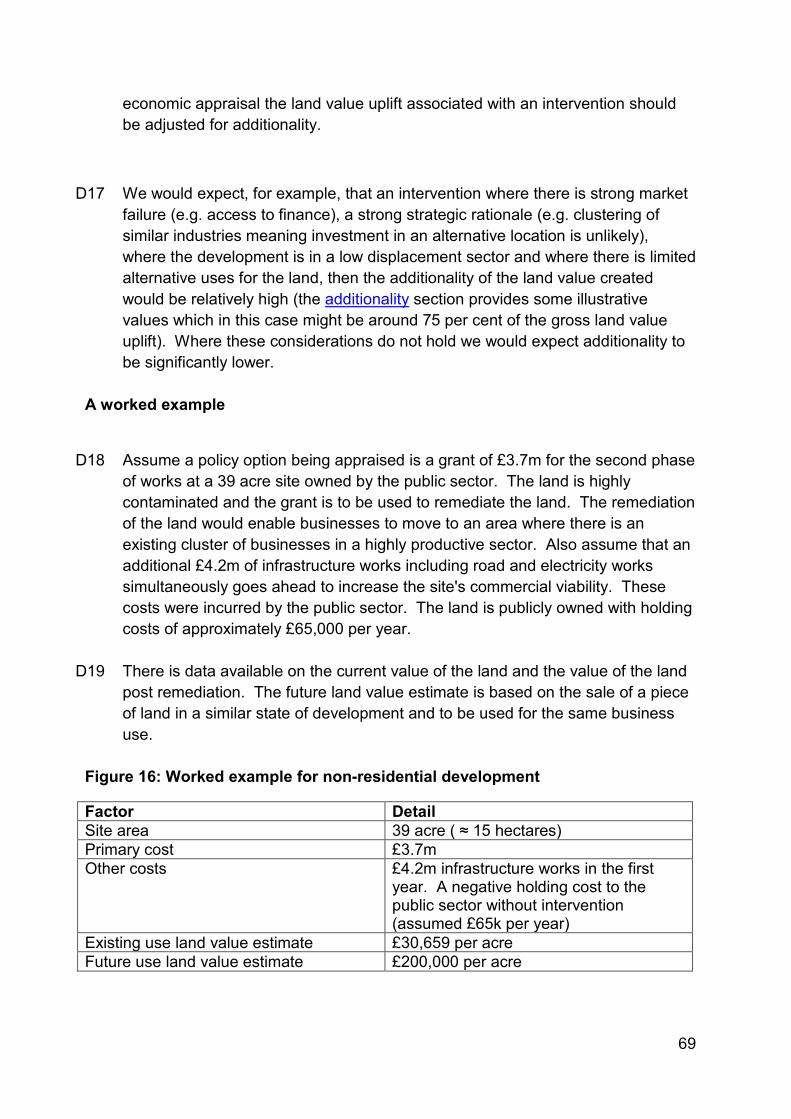
69

economic appraisal the land value uplift associated with an intervention should be adjusted for additionality.

D17 We would expect, for example, that an intervention where there is strong market failure (e.g. access to finance), a strong strategic rationale (e.g. clustering of similar industries meaning investment in an alternative location is unlikely), where the development is in a low displacement sector and where there is limited alternative uses for the land, then the additionality of the land value created would be relatively high (the additionality section provides some illustrative values which in this case might be around 75 per cent of the gross land value uplift). Where these considerations do not hold we would expect additionality to be significantly lower.

A worked example

D18 Assume a policy option being appraised is a grant of £3.7m for the second phase

of works at a 39 acre site owned by the public sector. The land is highly contaminated and the grant is to be used to remediate the land. The remediation of the land would enable businesses to move to an area where there is an existing cluster of businesses in a highly productive sector. Also assume that an additional £4.2m of infrastructure works including road and electricity works simultaneously goes ahead to increase the site's commercial viability. These costs were incurred by the public sector. The land is publicly owned with holding costs of approximately £65,000 per year.

D19 There is data available on the current value of the land and the value of the land

post remediation. The future land value estimate is based on the sale of a piece of land in a similar state of development and to be used for the same business use.

Figure 16: Worked example for non-residential development

Factor Detail Site area 39 acre ( ≈ 15 hectares) Primary cost £3.7m Other costs £4.2m infrastructure works in the first

year. A negative holding cost to the public sector without intervention (assumed £65k per year)

Existing use land value estimate £30,659 per acre Future use land value estimate £200,000 per acre

70

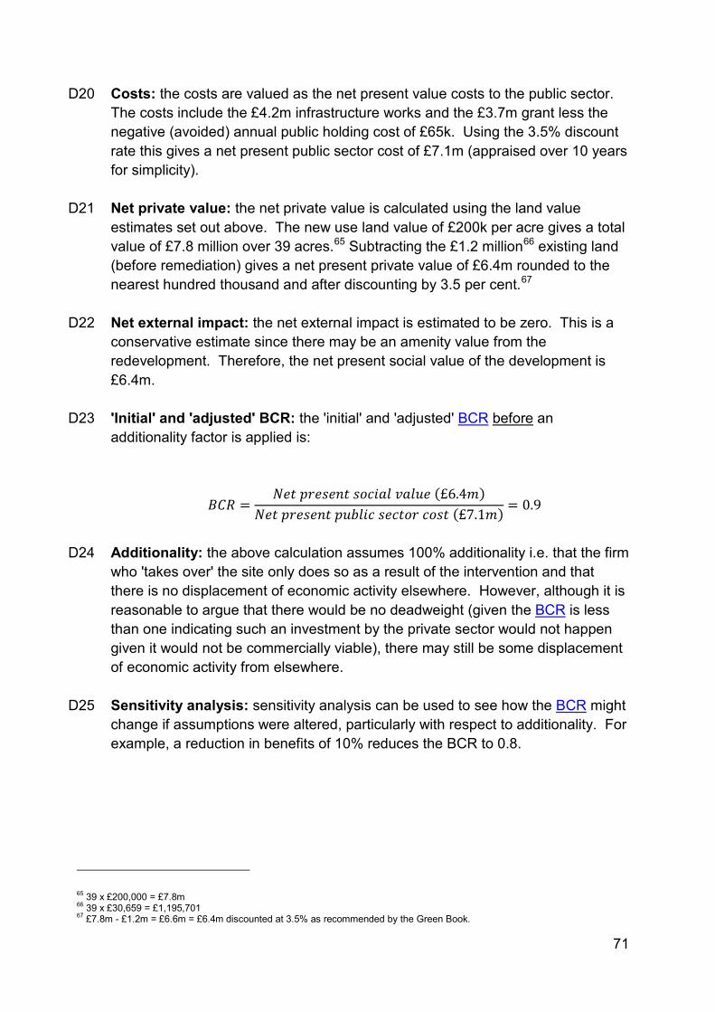
71

D20 Costs: the costs are valued as the net present value costs to the public sector. The costs include the £4.2m infrastructure works and the £3.7m grant less the negative (avoided) annual public holding cost of £65k. Using the 3.5% discount rate this gives a net present public sector cost of £7.1m (appraised over 10 years for simplicity).

D21 Net private value: the net private value is calculated using the land value estimates set out above. The new use land value of £200k per acre gives a total value of £7.8 million over 39 acres.65 Subtracting the £1.2 million66 existing land (before remediation) gives a net present private value of £6.4m rounded to the nearest hundred thousand and after discounting by 3.5 per cent.67

D22 Net external impact: the net external impact is estimated to be zero. This is a

conservative estimate since there may be an amenity value from the redevelopment. Therefore, the net present social value of the development is £6.4m.

D23 'Initial' and 'adjusted' BCR: the 'initial' and 'adjusted' BCR before an

additionality factor is applied is:

𝐵𝐶𝑅 =𝑁𝑒𝑡 𝑝𝑟𝑒𝑠𝑒𝑛𝑡 𝑠𝑜𝑐𝑖𝑎𝑙 𝑣𝑎𝑙𝑢𝑒 (£6.4𝑚)

𝑁𝑒𝑡 𝑝𝑟𝑒𝑠𝑒𝑛𝑡 𝑝𝑢𝑏𝑙𝑖𝑐 𝑠𝑒𝑐𝑡𝑜𝑟 𝑐𝑜𝑠𝑡 (£7.1𝑚) = 0.9

D24 Additionality: the above calculation assumes 100% additionality i.e. that the firm

who 'takes over' the site only does so as a result of the intervention and that there is no displacement of economic activity elsewhere. However, although it is reasonable to argue that there would be no deadweight (given the BCR is less than one indicating such an investment by the private sector would not happen given it would not be commercially viable), there may still be some displacement of economic activity from elsewhere.

D25 Sensitivity analysis: sensitivity analysis can be used to see how the BCR might change if assumptions were altered, particularly with respect to additionality. For example, a reduction in benefits of 10% reduces the BCR to 0.8.

65 39 x £200,000 = £7.8m 66 39 x £30,659 = £1,195,701 67 £7.8m - £1.2m = £6.6m = £6.4m discounted at 3.5% as recommended by the Green Book.

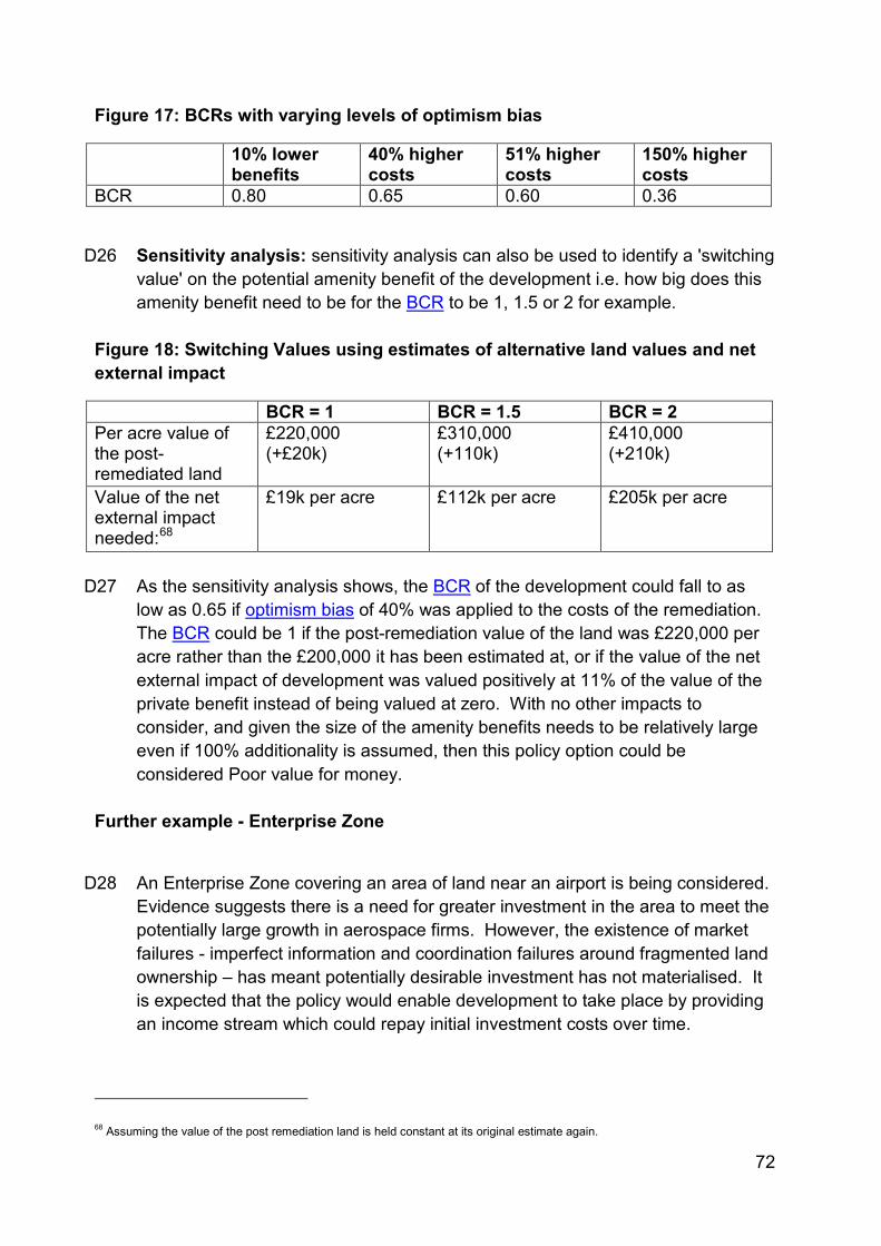
72

Figure 17: BCRs with varying levels of optimism bias

10% lower benefits

40% higher costs

51% higher costs

150% higher costs

BCR 0.80 0.65 0.60 0.36

D26 Sensitivity analysis: sensitivity analysis can also be used to identify a 'switching value' on the potential amenity benefit of the development i.e. how big does this amenity benefit need to be for the BCR to be 1, 1.5 or 2 for example.

Figure 18: Switching Values using estimates of alternative land values and net external impact

BCR = 1 BCR = 1.5 BCR = 2 Per acre value of the post-remediated land

£220,000 (+£20k)

£310,000 (+110k)

£410,000 (+210k)

Value of the net external impact needed:68

£19k per acre £112k per acre £205k per acre

D27 As the sensitivity analysis shows, the BCR of the development could fall to as

low as 0.65 if optimism bias of 40% was applied to the costs of the remediation. The BCR could be 1 if the post-remediation value of the land was £220,000 per acre rather than the £200,000 it has been estimated at, or if the value of the net external impact of development was valued positively at 11% of the value of the private benefit instead of being valued at zero. With no other impacts to consider, and given the size of the amenity benefits needs to be relatively large even if 100% additionality is assumed, then this policy option could be considered Poor value for money.

Further example - Enterprise Zone

D28 An Enterprise Zone covering an area of land near an airport is being considered.

Evidence suggests there is a need for greater investment in the area to meet the potentially large growth in aerospace firms. However, the existence of market failures - imperfect information and coordination failures around fragmented land ownership – has meant potentially desirable investment has not materialised. It is expected that the policy would enable development to take place by providing an income stream which could repay initial investment costs over time.

68 Assuming the value of the post remediation land is held constant at its original estimate again.

73

D29 The land value uplift of the proposal is estimated to be £540m (excluding the effect of any government support). The public cost is the estimated capital costs of £146m and business rate changes which are estimated to be £144m (meaning a £290m total public sector cost). Given (a) there is limited alternative uses for the land (b) there are strategic arguments for any investment to be near an airport and (c) the aerospace sector being appraised (which is likely to suffer from relatively small displacement), a 90% additionality factor is assumed. This level of additionality gives a net land value uplift of £486m (£540m x 90%). The present value benefits are therefore the additional land value uplift created of £486m plus the private benefit of the business rate changes, £144m. This gives a total benefit of £630m. The total costs are estimated to be £290m. Therefore, the NPPV is £340m and the BCR is 2.17.

Further example - Retail and Office development

D30 A new commercial development consisting of retail and office space is expected

in an urban area. This investment is forecast to be unlocked by a transport scheme. Analysis of local land value data suggests the non-transport development costs to be around £2.4bn, the estimated profit to firms be £0.7bn and the GDV to be £3.3bn.

D31 The land value before the development is £200k suggesting the change in land

value from the development to be £0.18bn (£3.3bn-£2.4bn-£0.7bn-£200k). However, given the transport appraisal captures the transport benefits of the proposal, a significant amount of the land value uplift is likely to be reflected in these transport benefits. Therefore, a low level of additionality is applied to the welfare impact of the number of houses unlocked (25%) and to the level of commercial development (10%). The weighted average level of the additionality is 21%. Given these assumptions, the additional land value created is therefore estimated to be £37.8m (£0.18bn x 21%). The external benefit of this unlocked development is estimated to be £22.2m suggesting a net social value for this development to be around £60m.

74

Annex E – Estimating value for money for non-residential development using land value uplift numbers where available

E1 This annex provides an approach to valuing the impacts of non-residential

development in the absence of local data and is aligned to transport guidance on assessing dependent development.

The approach

E2 The value to society of a planning decision to grant permission for new non-

residential development may be separated into two elements:

• The private benefit associated with the change in land use, as represented by the uplift in land value arising from the land moving from its current use to a more productive use. This uplift is defined as the value of the land in its new use (in this case commercial) minus the value of the land in its existing use (e.g. agriculture);

• net external impact of the resulting development, including any loss or gain in amenity.

E3 The equation below summarises this:

𝑁𝑒𝑡 𝑝𝑟𝑖𝑣𝑎𝑡𝑒 𝑣𝑎𝑙𝑢𝑒 𝑜𝑓 𝑛𝑜𝑛 − 𝑟𝑒𝑠𝑖𝑑𝑒𝑛𝑡𝑖𝑎𝑙 𝑑𝑒𝑣𝑒𝑙𝑜𝑝𝑚𝑒𝑛𝑡= 𝐶𝑜𝑚𝑚𝑒𝑟𝑐𝑖𝑎𝑙 𝑙𝑎𝑛𝑑 𝑣𝑎𝑙𝑢𝑒 (1) − 𝐸𝑥𝑖𝑠𝑡𝑖𝑛𝑔 𝑙𝑎𝑛𝑑 𝑢𝑠𝑒 𝑣𝑎𝑙𝑢𝑒 (2)

𝑁𝑒𝑡 𝑠𝑜𝑐𝑖𝑎𝑙 𝑣𝑎𝑙𝑢𝑒 𝑜𝑓 𝑛𝑜𝑛 − 𝑟𝑒𝑠𝑖𝑑𝑒𝑛𝑡𝑖𝑎𝑙 𝑑𝑒𝑣𝑒𝑙𝑜𝑝𝑚𝑒𝑛𝑡= 𝑁𝑒𝑡 𝑝𝑟𝑖𝑣𝑎𝑡𝑒 𝑣𝑎𝑙𝑢𝑒 𝑜𝑓 𝑛𝑜𝑛 − 𝑟𝑒𝑠𝑖𝑑𝑒𝑛𝑡𝑖𝑎𝑙 𝑑𝑒𝑣𝑒𝑙𝑜𝑝𝑚𝑒𝑛𝑡+ 𝑁𝑒𝑡 𝑒𝑥𝑡𝑒𝑟𝑛𝑎𝑙 𝑖𝑚𝑝𝑎𝑐𝑡 𝑜𝑓 𝑛𝑜𝑛 − 𝑟𝑒𝑠𝑖𝑑𝑒𝑛𝑡𝑖𝑎𝑙 𝑑𝑒𝑣𝑒𝑙𝑜𝑝𝑚𝑒𝑛𝑡 (3)

The calculation

E4 Below is a discussion of the key elements of the appraisal, including the data

inputs and underlying assumptions. Note that a number of data inputs must be specified by the user on a case-by-case basis as they relate to the nature of the development in question.

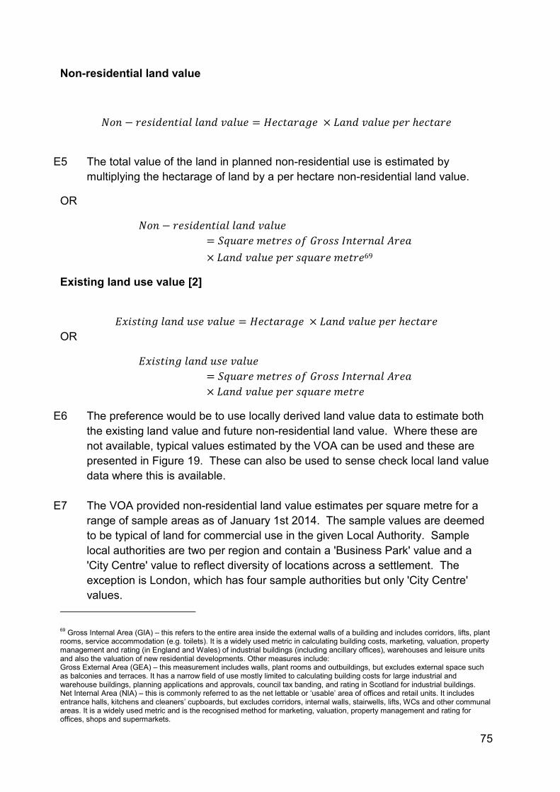
75

Non-residential land value

𝑁𝑜𝑛 − 𝑟𝑒𝑠𝑖𝑑𝑒𝑛𝑡𝑖𝑎𝑙 𝑙𝑎𝑛𝑑 𝑣𝑎𝑙𝑢𝑒 = 𝐻𝑒𝑐𝑡𝑎𝑟𝑎𝑔𝑒 × 𝐿𝑎𝑛𝑑 𝑣𝑎𝑙𝑢𝑒 𝑝𝑒𝑟 ℎ𝑒𝑐𝑡𝑎𝑟𝑒

E5 The total value of the land in planned non-residential use is estimated by

multiplying the hectarage of land by a per hectare non-residential land value.

OR

𝑁𝑜𝑛 − 𝑟𝑒𝑠𝑖𝑑𝑒𝑛𝑡𝑖𝑎𝑙 𝑙𝑎𝑛𝑑 𝑣𝑎𝑙𝑢𝑒= 𝑆𝑞𝑢𝑎𝑟𝑒 𝑚𝑒𝑡𝑟𝑒𝑠 𝑜𝑓 𝐺𝑟𝑜𝑠𝑠 𝐼𝑛𝑡𝑒𝑟𝑛𝑎𝑙 𝐴𝑟𝑒𝑎 × 𝐿𝑎𝑛𝑑 𝑣𝑎𝑙𝑢𝑒 𝑝𝑒𝑟 𝑠𝑞𝑢𝑎𝑟𝑒 𝑚𝑒𝑡𝑟𝑒69

Existing land use value [2]

𝐸𝑥𝑖𝑠𝑡𝑖𝑛𝑔 𝑙𝑎𝑛𝑑 𝑢𝑠𝑒 𝑣𝑎𝑙𝑢𝑒 = 𝐻𝑒𝑐𝑡𝑎𝑟𝑎𝑔𝑒 × 𝐿𝑎𝑛𝑑 𝑣𝑎𝑙𝑢𝑒 𝑝𝑒𝑟 ℎ𝑒𝑐𝑡𝑎𝑟𝑒

OR

𝐸𝑥𝑖𝑠𝑡𝑖𝑛𝑔 𝑙𝑎𝑛𝑑 𝑢𝑠𝑒 𝑣𝑎𝑙𝑢𝑒= 𝑆𝑞𝑢𝑎𝑟𝑒 𝑚𝑒𝑡𝑟𝑒𝑠 𝑜𝑓 𝐺𝑟𝑜𝑠𝑠 𝐼𝑛𝑡𝑒𝑟𝑛𝑎𝑙 𝐴𝑟𝑒𝑎 × 𝐿𝑎𝑛𝑑 𝑣𝑎𝑙𝑢𝑒 𝑝𝑒𝑟 𝑠𝑞𝑢𝑎𝑟𝑒 𝑚𝑒𝑡𝑟𝑒

E6 The preference would be to use locally derived land value data to estimate both the existing land value and future non-residential land value. Where these are not available, typical values estimated by the VOA can be used and these are presented in Figure 19. These can also be used to sense check local land value data where this is available.

E7 The VOA provided non-residential land value estimates per square metre for a range of sample areas as of January 1st 2014. The sample values are deemed to be typical of land for commercial use in the given Local Authority. Sample local authorities are two per region and contain a 'Business Park' value and a 'City Centre' value to reflect diversity of locations across a settlement. The exception is London, which has four sample authorities but only 'City Centre' values.

69 Gross Internal Area (GIA) – this refers to the entire area inside the external walls of a building and includes corridors, lifts, plant rooms, service accommodation (e.g. toilets). It is a widely used metric in calculating building costs, marketing, valuation, property management and rating (in England and Wales) of industrial buildings (including ancillary offices), warehouses and leisure units and also the valuation of new residential developments. Other measures include: Gross External Area (GEA) – this measurement includes walls, plant rooms and outbuildings, but excludes external space such as balconies and terraces. It has a narrow field of use mostly limited to calculating building costs for large industrial and warehouse buildings, planning applications and approvals, council tax banding, and rating in Scotland for industrial buildings. Net Internal Area (NIA) – this is commonly referred to as the net lettable or ‘usable’ area of offices and retail units. It includes entrance halls, kitchens and cleaners’ cupboards, but excludes corridors, internal walls, stairwells, lifts, WCs and other communal areas. It is a widely used metric and is the recognised method for marketing, valuation, property management and rating for offices, shops and supermarkets.

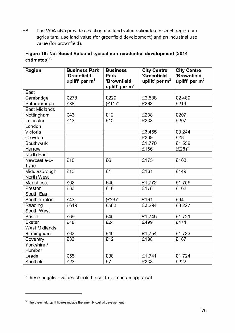
76

E8 The VOA also provides existing use land value estimates for each region: an agricultural use land value (for greenfield development) and an industrial use value (for brownfield).

Figure 19: Net Social Value of typical non-residential development (2014 estimates)70

Region Business Park 'Greenfield uplift' per m2

Business Park 'Brownfield uplift' per m2

City Centre 'Greenfield uplift' per m2

City Centre 'Brownfield uplift' per m2

East Cambridge £278 £229 £2,538 £2,489 Peterborough £38 (£11)* £263 £214 East Midlands Nottingham £43 £12 £238 £207 Leicester £43 £12 £238 £207 London Victoria £3,455 £3,244 Croydon £239 £28 Southwark £1,770 £1,559 Harrow £186 (£26)* North East Newcastle-u-Tyne

£18 £6 £175 £163

Middlesbrough £13 £1 £161 £149 North West Manchester £62 £46 £1,772 £1,756 Preston £33 £16 £178 £162 South East Southampton £43 (£23)* £161 £94 Reading £649 £583 £3,294 £3,227 South West Bristol £69 £45 £1,745 £1,721 Exeter £48 £24 £499 £474 West Midlands Birmingham £62 £40 £1,754 £1,733 Coventry £33 £12 £188 £167 Yorkshire / Humber

Leeds £55 £38 £1,741 £1,724 Sheffield £23 £7 £238 £222

* these negative values should be set to zero in an appraisal

70 The greenfield uplift figures include the amenity cost of development.

77

E9 VOA's non- residential land values should be regarded as illustrative, and represent typical levels of value for sites for development, in that they have the following conditions:

• no abnormal site constraints;

• a residential planning permission of a type generally found in the area;

• services to the edge of the site

E10 VOA's reported land values should be regarded as being at market prices (i.e.

gross of indirect tax).

E11 In practice, land values vary substantially on a site-by-site basis, given differences in, for example, proximity to amenities or density of development. Users are therefore encouraged to draw upon alternative sources of evidence to inform estimates of land values.

E12 In using these values, users will need to make a choice from:

• Two site values per region or four in the case of London;

• Site value based on whether the land was brownfield or greenfield;

• Site value based on whether the non-residential development is in the city centre or business park.

E13 The economic case should clearly set out the justification for choices made.

Net external impact of non-residential development [3]

𝑁𝑒𝑡 𝑒𝑥𝑡𝑒𝑟𝑛𝑎𝑙 𝑖𝑚𝑝𝑎𝑐𝑡 𝑜𝑓 𝑛𝑜𝑛 − 𝑟𝑒𝑠𝑖𝑑𝑒𝑛𝑡𝑖𝑎𝑙 𝑑𝑒𝑣𝑒𝑙𝑜𝑝𝑚𝑒𝑛𝑡= [𝐻𝑒𝑐𝑡𝑎𝑟𝑎𝑔𝑒 × (𝑝𝑒𝑟 ℎ𝑒𝑐𝑡𝑎𝑟𝑒) 𝐸𝑥𝑡𝑒𝑟𝑛𝑎𝑙 𝑖𝑚𝑝𝑎𝑐𝑡 𝑜𝑓 𝑎 𝑑𝑒𝑣𝑒𝑙𝑜𝑝𝑚𝑒𝑛𝑡]+ 𝑇𝑟𝑎𝑛𝑠𝑝𝑜𝑟𝑡 𝑟𝑒𝑙𝑎𝑡𝑒𝑑 𝑒𝑥𝑡𝑒𝑟𝑛𝑎𝑙 𝑖𝑚𝑝𝑎𝑐𝑡 𝑜𝑓 𝑎 𝑑𝑒𝑣𝑒𝑙𝑜𝑝𝑚𝑒𝑛𝑡

78

E14 Users may draw upon alternative sources of evidence to inform estimation of external impacts of development. For greenfield site developments a value per square metre is attributed to the development based on the estimated change in amenity value from developing a greenfield site.

E15 The overall benefits related to the development are therefore:

𝑇ℎ𝑒 𝑛𝑒𝑡 𝑠𝑜𝑐𝑖𝑎𝑙 𝑣𝑎𝑙𝑢𝑒 𝑜𝑓 𝑡ℎ𝑒 𝑑𝑒𝑣𝑒𝑙𝑜𝑝𝑚𝑒𝑛𝑡 = 𝑁𝑒𝑡 𝑝𝑟𝑖𝑣𝑎𝑡𝑒 𝑣𝑎𝑙𝑢𝑒 𝑜𝑓 𝑛𝑜𝑛 − 𝑟𝑒𝑠𝑖𝑑𝑒𝑛𝑡𝑖𝑎𝑙 𝑑𝑒𝑣𝑒𝑙𝑜𝑝𝑚𝑒𝑛𝑡 (1 − 2)+ 𝑁𝑒𝑡 𝑒𝑥𝑡𝑒𝑟𝑛𝑎𝑙 𝑖𝑚𝑝𝑎𝑐𝑡 𝑜𝑓 𝑛𝑜𝑛 − 𝑟𝑒𝑠𝑖𝑑𝑒𝑛𝑡𝑖𝑎𝑙 𝑑𝑒𝑣𝑒𝑙𝑜𝑝𝑚𝑒𝑛𝑡 (3)

E16 In which the land value uplift estimate captures the net private benefits and the

net external impact captures externalities such as changes in amenity. Costs

E17 All public sector costs should be included in the present value costs. If the land

is owned by the public sector then the public sector will be incurring holding costs assumed to be 2 per cent of the existing value of the land per year. Should the land be used for non-residential development these holding costs will be avoided. This needs to be reflected in the appraisal as a negative cost. Any private costs associated with the development should be included in the appraisal as a dis-benefit and therefore feature in the numerator of the BCR calculation.

Appraisal period

E18 We would expect this to be 10, 30 or 60 years depending on the intervention

being appraised. Timing

E19 The land value uplift is assumed to happen at the same time as a change in land

use. There is no assumption that benefits are built slowly over a specified time period. As the land value figures provided by the VOA are likely to be for a fixed time in the year these will need to be inflated to reflect prices at the time of the change in land use. The current assumption is 5 per cent per year.

E20 All other costs and benefits will need to be discounted at 3.5 per cent in line with the Green Book.

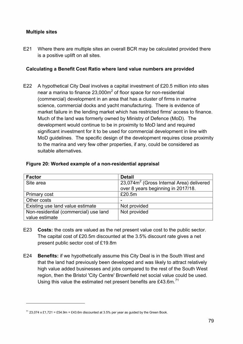
79

Multiple sites

E21 Where there are multiple sites an overall BCR may be calculated provided there

is a positive uplift on all sites. Calculating a Benefit Cost Ratio where land value numbers are provided

E22 A hypothetical City Deal involves a capital investment of £20.5 million into sites

near a marina to finance 23,000m2 of floor space for non-residential (commercial) development in an area that has a cluster of firms in marine science, commercial docks and yacht manufacturing. There is evidence of market failure in the lending market which has restricted firms' access to finance. Much of the land was formerly owned by Ministry of Defence (MoD). The development would continue to be in proximity to MoD land and required significant investment for it to be used for commercial development in line with MoD guidelines. The specific design of the development requires close proximity to the marina and very few other properties, if any, could be considered as suitable alternatives.

Figure 20: Worked example of a non-residential appraisal Factor Detail Site area 23,074m2 (Gross Internal Area) delivered

over 8 years beginning in 2017/18. Primary cost £20.5m Other costs - Existing use land value estimate Not provided Non-residential (commercial) use land value estimate

Not provided

E23 Costs: the costs are valued as the net present value cost to the public sector.

The capital cost of £20.5m discounted at the 3.5% discount rate gives a net present public sector cost of £19.8m

E24 Benefits: if we hypothetically assume this City Deal is in the South West and that the land had previously been developed and was likely to attract relatively high value added businesses and jobs compared to the rest of the South West region, then the Bristol 'City Centre' Brownfield net social value could be used. Using this value the estimated net present benefits are £43.6m.71

71 23,074 x £1,721 = £54.9m = £43.6m discounted at 3.5% per year as guided by the Green Book.

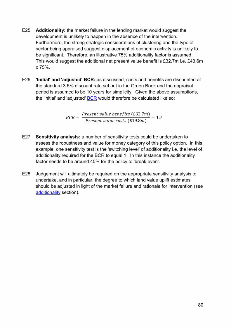
80

E25 Additionality: the market failure in the lending market would suggest the development is unlikely to happen in the absence of the intervention. Furthermore, the strong strategic considerations of clustering and the type of sector being appraised suggest displacement of economic activity is unlikely to be significant. Therefore, an illustrative 75% additionality factor is assumed. This would suggest the additional net present value benefit is £32.7m i.e. £43.6m x 75%.

E26 'Initial' and 'adjusted' BCR: as discussed, costs and benefits are discounted at

the standard 3.5% discount rate set out in the Green Book and the appraisal period is assumed to be 10 years for simplicity. Given the above assumptions, the 'initial' and 'adjusted' BCR would therefore be calculated like so:

𝐵𝐶𝑅 = 𝑃𝑟𝑒𝑠𝑒𝑛𝑡 𝑣𝑎𝑙𝑢𝑒 𝑏𝑒𝑛𝑒𝑓𝑖𝑡𝑠 (£32.7𝑚)𝑃𝑟𝑒𝑠𝑒𝑛𝑡 𝑣𝑎𝑙𝑢𝑒 𝑐𝑜𝑠𝑡𝑠 (£19.8𝑚)

= 1.7

E27 Sensitivity analysis: a number of sensitivity tests could be undertaken to

assess the robustness and value for money category of this policy option. In this example, one sensitivity test is the 'switching level' of additionality i.e. the level of additionality required for the BCR to equal 1. In this instance the additionality factor needs to be around 45% for the policy to 'break even'.

E28 Judgement will ultimately be required on the appropriate sensitivity analysis to undertake, and in particular, the degree to which land value uplift estimates should be adjusted in light of the market failure and rationale for intervention (see additionality section).

81

Annex F – Externalities associated with development Background

F1 An economic appraisal should seek to capture all the benefits and costs of an

intervention. Therefore, any external benefits and external costs should be included in addition to the estimated net private impacts. To account for such impacts, users should draw on appropriate evidence and guidance to value these impacts.

F2 For DCLG appraisals, to ensure consistency and transparency on what is

included in an economic appraisal, only impacts that can be robustly valued using (Supplementary and Departmental) Green Book guidance should be included in the estimate of an 'initial' BCR. Examples of such impacts include greenhouse gas emissions and other environmental impacts such as amenity costs of development as well as crime, transport and health impacts.72 Distributional impacts and other impacts should be monetised separately and included in an 'adjusted' BCR.

F3 For many DCLG appraisals, land value uplift will represent a significant

proportion of private benefits. However, as with all methods, there is a need to account for external impacts, preferably through monetisation.

F4 There are a number of external impacts that are likely to result from a

development including potential agglomeration impacts on third parties, health impacts of additional affordable housing and brownfield land clean-up, educational impacts of additional housing, transport externalities, public realm impacts, environmental impacts, and cultural and amenity impacts of development.

F5 However, the evidence base for some of these externalities needs developing

and so further research is needed before they can be included in the 'initial' BCR. However, estimates for these externalities should still form part of the appraisal and be included in the 'adjusted' BCR.

F6 To help guide users, this annex provides an illustrative external impact for the

external benefit of additional affordable housing. This estimate could feature in the 'adjusted' BCR. However, this externality is 'in development' and is therefore subject to change as further evidence becomes available.

72 See the following link for supplementary Green Book guidance: https://www.gov.uk/government/publications/the-green-book-appraisal-and-evaluation-in-central-governent

82

F7 We plan to develop appraisal values for agglomeration impacts on third parties and transport externalities associated with development. However, given DfT are updating their wider economic benefits guidance (which includes agglomeration impacts) the department has concluded that it would be more appropriate to develop an estimate of the potential agglomeration impact of new development in line with this update. It will therefore feature in a future version of the DCLG Appraisal Guide.

Determining whether an impact is an externality

F8 When assessing externalities, it is important to consider whether an impact is

already captured in land value uplift and therefore an additional impact which needs to be monetised. The framework below in Figure 21 sets out an approach to do this.

F9 The key question to ask of a potential impact is "who does it affect?" If the

impact affects the welfare of an individual or firm moving to an area, then this impact may be fully reflected in price they pay for the land. Where this is the case, these impacts should not be considered an externality. If the impact affects the welfare of individuals or firms already in the area, then this impact will not be accounted for in land value uplift and is therefore an externality. If the impact affects society as a whole (so not exclusively existing individuals or firms in an area), then this impact will not be accounted for in land value uplift and is therefore an externality.

F10 The basis for this is that a firm will consider the returns from all factors of

production when making a decision to locate in a particular area. It will therefore consider whether there are any potential spill-over benefits to them from co-location with other firms (agglomeration impacts) and the costs to the firm from higher congestion. For individuals moving to an area, they will also factor in any potential congestion costs and any health, education or amenity benefits they may derive from such a move so this may also already be factored into land value uplift.

F11 However, land value uplift will not account for impacts which affect existing firms or individuals in an area (or society as a whole). These are externalities. For example, any knowledge spill-over impacts enjoyed by other firms will not be taken into account by the firm deciding to locate in an area so are in addition to land value uplift. Similarly, the firm or individual deciding to locate in an area will not take into account the congestion cost they impose on others or the environmental impact of their decisions. These impacts are externalities which need to be accounted for in addition to land value uplift.

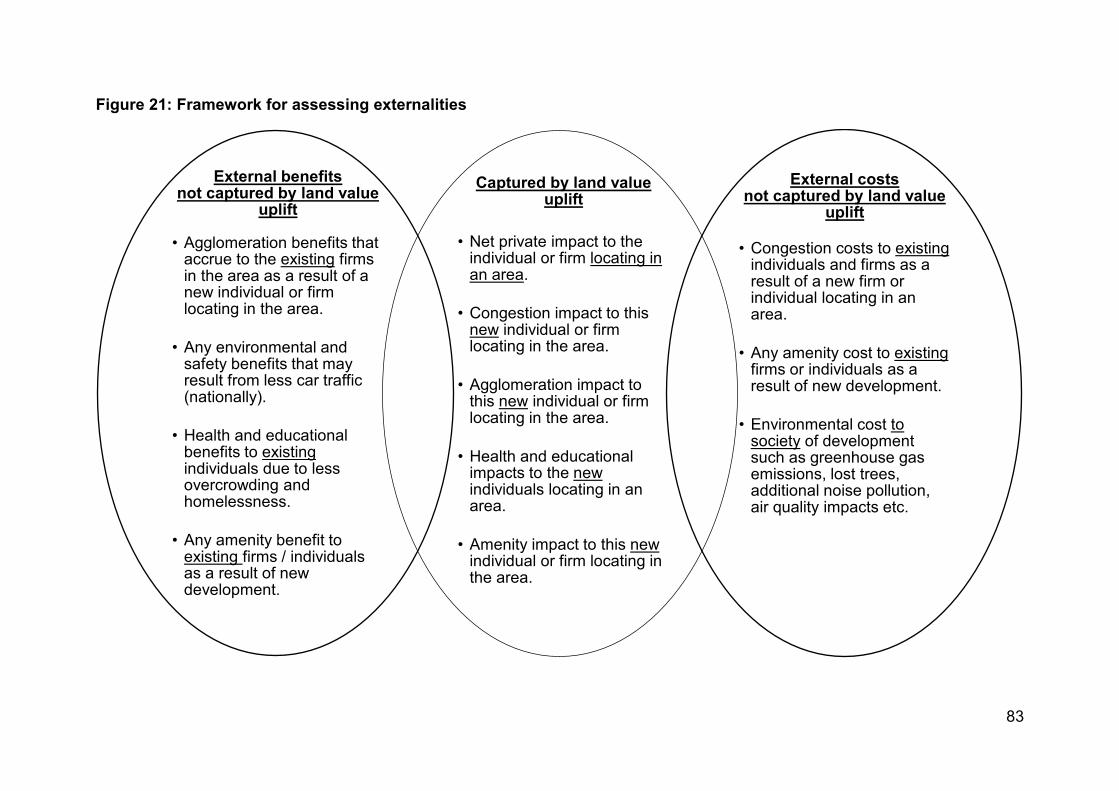
83

Figure 21: Framework for assessing externalities

External benefits not captured by land value

uplift

• Agglomeration benefits that accrue to the existing firms in the area as a result of a new individual or firm locating in the area.

• Any environmental and safety benefits that may result from less car traffic (nationally).

• Health and educational benefits to existing individuals due to less overcrowding and homelessness.

• Any amenity benefit to existing firms / individuals as a result of new development.

Captured by land value

uplift

• Net private impact to the individual or firm locating in an area.

• Congestion impact to this new individual or firm locating in the area.

• Agglomeration impact to this new individual or firm locating in the area.

• Health and educational impacts to the new individuals locating in an area.

• Amenity impact to this new individual or firm locating in the area.

External costs not captured by land value

uplift

• Congestion costs to existing individuals and firms as a result of a new firm or individual locating in an area.

• Any amenity cost to existing firms or individuals as a result of new development.

• Environmental cost to society of development such as greenhouse gas emissions, lost trees, additional noise pollution, air quality impacts etc.

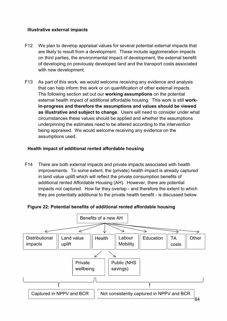
84

Illustrative external impacts

F12 We plan to develop appraisal values for several potential external impacts that

are likely to result from a development. These include agglomeration impacts on third parties, the environmental impact of development, the external benefit of developing on previously developed land and the transport costs associated with new development.

F13 As part of this work, we would welcome receiving any evidence and analysis that can help inform this work or on quantification of other external impacts. The following section set out our working assumptions on the potential external health impact of additional affordable housing. This work is still work-in-progress and therefore the assumptions and values should be viewed as illustrative and subject to change. Users will need to consider under what circumstances these values should be applied and whether the assumptions underpinning the estimates need to be altered according to the intervention being appraised. We would welcome receiving any evidence on the assumptions used.

Health impact of additional rented affordable housing

F14 There are both external impacts and private impacts associated with health

improvements. To some extent, the (private) health impact is already captured in land value uplift which will reflect the private consumption benefits of additional rented Affordable Housing (AH). However, there are potential impacts not captured. How far they overlap - and therefore the extent to which they are potentially additional to the private health benefit - is discussed below.

Figure 22: Potential benefits of additional rented affordable housing

Health Labour Mobility

Benefits of a new AH

Education Land value uplift

Private wellbeing

Public (NHS savings)

Distributional impacts

Captured in NPPV and BCR Not consistently captured in NPPV and BCR

Other TA costs

85

F15 As the diagram above illustrates, there are a number of benefits associated

with an additional rented AH unit. There is the private benefit – as measured by land value uplift which captures the efficiency benefit of converting land into a more productive use – and a potential distributional impact associated with the progressive nature of AH (see Annex G). Both these impacts are captured separately in an appraisal.

F16 However, there are also several impacts which are not monetised. These

include fiscal savings from the potential savings on health care, improved labour mobility – increased housing supply lowers housing costs and therefore enables people to live in areas they might otherwise not be able to live – and potentially improved educational outcomes by reducing overcrowding. Finally it can result in savings to exchequer from avoiding expensive temporary accommodation (TA) costs.

F17 This section focuses only on potential health impacts. Assessing the potential

significance of these impacts is problematic as these impacts are only likely to materialise if a new rented AH unit (a) enables a household to move away from a housing situation that was imposing an external cost and (b) another household does not then move into the same housing situation and instead this property is made either more habitable or could even be demolished (if the latter there may not be any land value uplift associated with the new rented AH unit as it would not be an additional housing unit).

F18 Therefore, in order to estimate the potential health impact of additional rented

affordable housing, the probability of a new tenant that had previously been living in a poor condition or overcrowded property needs to be calculated. In addition, as there are large negative health impacts from rough sleeping, an additional house that is allocated to a rough sleeper can be expected to deliver relatively large health impacts (currently around 1% of new lets go to previous rough sleepers). This should be factored into the probability calculations.73

Estimating probabilities

F19 In order to estimate the probability that a new tenant had previously been living

in either poor or overcrowded conditions, the following working assumptions have been made:

73 We have focussed on the impact of an additional affordable housing unit so have not accounted for the potential benefits of improving the condition of existing poor quality housing.

86

• Within the social rented sector (SRS), it has been assumed that those living in overcrowded accommodation are prioritised first;

• 10% of vacated properties are filled by a newly formed household (HH); and

• 1% of new lets go to rough sleepers (CORE data for 2014/15 shows around 1% of new lets to General Needs Private Registered Providers (PRP) are to those who say they were previously rough sleeping).

F20 The formula for estimating the probability that an additional dwelling reduces overcrowding is:

𝑃𝑟𝑜𝑏𝑎𝑏𝑖𝑙𝑖𝑡𝑦 𝑛𝑒𝑤 𝑢𝑛𝑖𝑡 𝑟𝑒𝑑𝑢𝑐𝑒𝑠 𝑜𝑣𝑒𝑟𝑐𝑟𝑜𝑤𝑑𝑖𝑛𝑔 == (99% − 10% ℎ𝑜𝑢𝑠𝑒ℎ𝑜𝑙𝑑 𝑓𝑜𝑟𝑚𝑎𝑡𝑖𝑜𝑛)

F21 The 99% assumption is derived from 100% less 1% of new lets going to rough

sleepers. The 10% HH formation assumption is the assumed proportion of new households forming as a result of building the new unit. Therefore, an additional house will, to some extent, lead to reduced overcrowding except where there is new HH formation.

Estimating the size of the external impacts

F22 The Building Research Establishment (TBRE) has developed a model to

estimate the impact of poor housing on the NHS. This is well established and their 2010 report has been widely quoted including by the World Health Organisation (WHO), National Housing Federation and Age UK. TBRE estimates the number of homes with Category 1 Housing Health and Safety Rating System (HHSRS) hazards and then estimates the cost to the NHS associated with them. There are 29 identified HHSRS hazards, including the risks from cold, damp, falls on stairs etc.

F23 The study estimates the direct (medical) costs to the NHS that are likely to result from the presence of these hazards, using NHS data on costs of treating and caring for related health conditions up to a year following a health incident.

87

F24 TBRE updated the model in 2014 and their briefing paper on the revised findings published in 2015 reveals that leaving vulnerable people in the poorest 15% of England’s housing costs the NHS £1.4 billion per annum in first year treatment costs. The full report of the findings to be published in 2016 will contain findings on the impact of all substandard dwellings, and include wider impacts on peoples' life chances following a housing related incident, as well as the immediate medical costs. Initial estimates imply that the medical costs above are at best 40% of the total cost of society – which are given as £3.5bn. The methodology of the 2010 model is outlined in the TBRE Information Paper 'Quantifying the cost of poor housing.'

F25 Although the TBRE’s method is well known, these are impacts for improving the

conditions of the worst 15% of housing, which is different to building a new unit. This is where the probability section becomes relevant. Using unit impacts from the table below with some example probabilities gives some indicative health impacts:

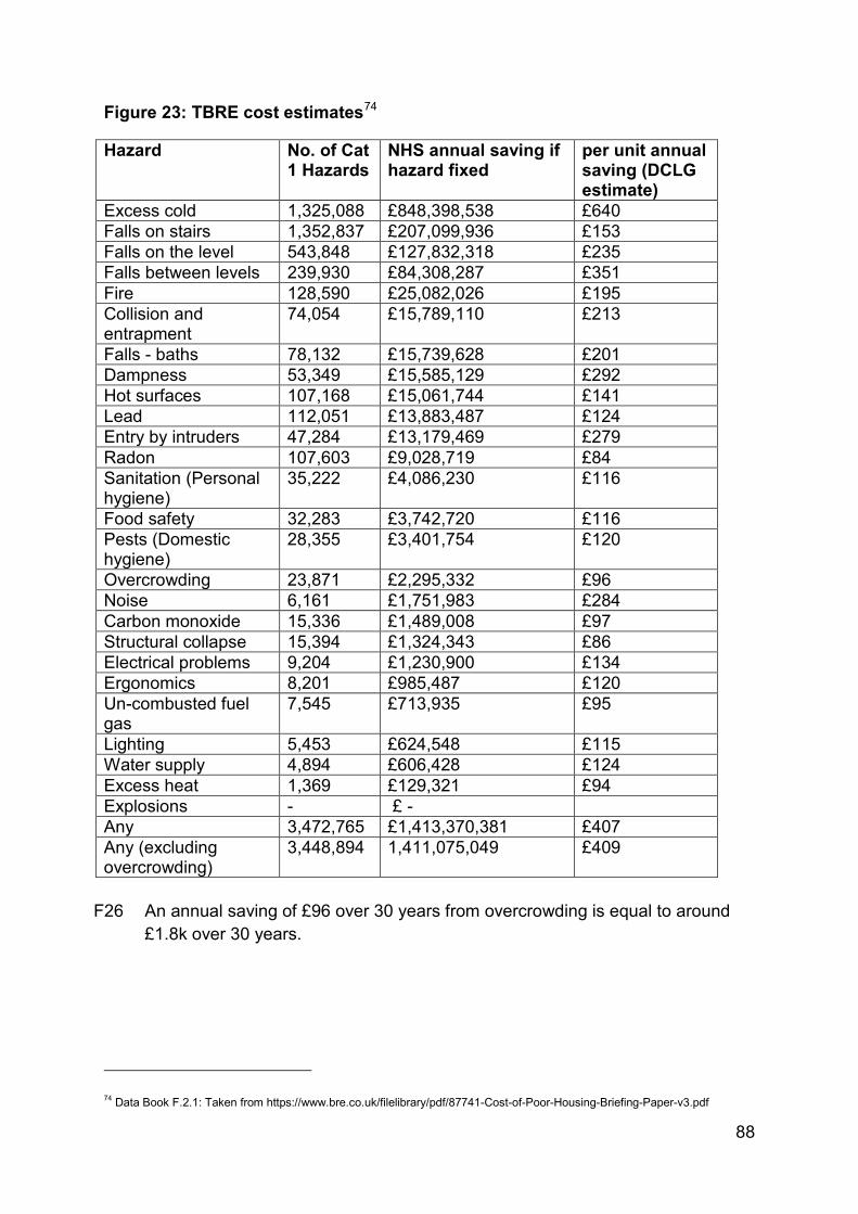
88

Figure 23: TBRE cost estimates74

Hazard No. of Cat 1 Hazards

NHS annual saving if hazard fixed

per unit annual saving (DCLG estimate)

Excess cold 1,325,088 £848,398,538 £640 Falls on stairs 1,352,837 £207,099,936 £153 Falls on the level 543,848 £127,832,318 £235 Falls between levels 239,930 £84,308,287 £351 Fire 128,590 £25,082,026 £195 Collision and entrapment

74,054 £15,789,110 £213

Falls - baths 78,132 £15,739,628 £201 Dampness 53,349 £15,585,129 £292 Hot surfaces 107,168 £15,061,744 £141 Lead 112,051 £13,883,487 £124 Entry by intruders 47,284 £13,179,469 £279 Radon 107,603 £9,028,719 £84 Sanitation (Personal hygiene)

35,222 £4,086,230 £116

Food safety 32,283 £3,742,720 £116 Pests (Domestic hygiene)

28,355 £3,401,754 £120

Overcrowding 23,871 £2,295,332 £96 Noise 6,161 £1,751,983 £284 Carbon monoxide 15,336 £1,489,008 £97 Structural collapse 15,394 £1,324,343 £86 Electrical problems 9,204 £1,230,900 £134 Ergonomics 8,201 £985,487 £120 Un-combusted fuel gas

7,545 £713,935 £95

Lighting 5,453 £624,548 £115 Water supply 4,894 £606,428 £124 Excess heat 1,369 £129,321 £94 Explosions - £ - Any 3,472,765 £1,413,370,381 £407 Any (excluding overcrowding)

3,448,894 1,411,075,049 £409

F26 An annual saving of £96 over 30 years from overcrowding is equal to around

£1.8k over 30 years.

74 Data Book F.2.1: Taken from https://www.bre.co.uk/filelibrary/pdf/87741-Cost-of-Poor-Housing-Briefing-Paper-v3.pdf

89

Homelessness evidence

F27 Estimates for the typical per-person cost of the health impacts of homelessness

vary, as do estimates of the costs that remain even if they are housed.

F28 There is evidence on health costs for rough sleepers and for those with severe and multiple deprivation. Whilst we only account for the health benefits from rough sleepers here, some of the estimates used are for a broader definition of homeless than just rough sleepers, who may be expected to have higher health costs than other homelessness types which would mean these estimates may be an underestimate. There may also be additional health costs for other types of homeless people accessing social housing that could be considered on top of these.

F29 Estimates for the costs per person per year range from £2,000 to £19,000, with

an average of around £7,500.75 Sources vary, from incidence rates and illustrative scenarios combined with unit costs, to survey data of particular interventions.

F30 Some of these costs are likely to remain even once someone is housed. We

have considered two approaches for how to account for this. The first is to subtract the average cost of the general population’s use of the same health services, which is around £1,000 per person per year, suggesting a net saving on health of around £6,500. This is likely to be to an overestimate of the savings, as former rough sleepers may be expected to have more health problems than the general population.

F31 The second approach is to only count 27% of the gross costs as being avoided once the rough sleeper is housed, in line with Larimer et al (2009) which would give a net saving on health of around £2,200 per person per year in this case. This may be an underestimate of savings, as the source for the 27% estimate was a study of the chronically homeless with severe alcohol problems (whereas those rough sleepers accessing social housing are likely to have fewer problems than that group). Our working assumption is to take the average of the two approaches which gives a net saving on health costs of around £4,000.

Final calculation

F32 The formula for estimating the external health impacts from additional rented

affordable housing is therefore:

75 Data Book F.2.2: A list of sources is given in the bibliography and in the Data Book

90

𝐴𝑛𝑛𝑢𝑎𝑙 ℎ𝑒𝑎𝑙𝑡ℎ 𝑖𝑚𝑝𝑎𝑐𝑡= 𝐼𝑚𝑝𝑎𝑐𝑡 𝑜𝑓 𝑟𝑒𝑑𝑢𝑐𝑒𝑑 𝑜𝑣𝑒𝑟𝑐𝑟𝑜𝑤𝑑𝑖𝑛𝑔× 𝑝𝑟𝑜𝑏𝑎𝑏𝑖𝑙𝑖𝑡𝑦 𝑜𝑓 𝑛𝑒𝑤 𝑢𝑛𝑖𝑡 𝑟𝑒𝑑𝑢𝑐𝑒𝑠 𝑜𝑣𝑒𝑟𝑐𝑟𝑜𝑤𝑑𝑖𝑛𝑔+ 𝐼𝑚𝑝𝑎𝑐𝑡 𝑜𝑓 𝑟𝑒𝑑𝑢𝑐𝑒𝑑 𝑟𝑜𝑢𝑔ℎ 𝑠𝑙𝑒𝑒𝑝𝑖𝑛𝑔× 𝑝𝑟𝑜𝑏𝑎𝑏𝑖𝑙𝑖𝑡𝑦 𝑛𝑒𝑤 𝑢𝑛𝑖𝑡 𝑟𝑒𝑑𝑢𝑐𝑒𝑠 ℎ𝑜𝑚𝑒𝑙𝑒𝑠𝑠𝑛𝑒𝑠𝑠= £96 × (99% − 10% ℎ𝑜𝑢𝑠𝑒ℎ𝑜𝑙𝑑 𝑓𝑜𝑟𝑚𝑎𝑡𝑖𝑜𝑛) + £4,000× 1% 𝑟𝑒𝑑𝑢𝑐𝑒𝑑 ℎ𝑜𝑚𝑒𝑙𝑒𝑠𝑠𝑛𝑒𝑠𝑠

F33 Essentially the annual health impact is the annual £4,000 health care cost multiplied by the probability that someone is a former rough sleeper (1%) plus the probability of a new rented AH unit reducing overcrowding (89%) multiplied by the annual impact of reduced overcrowding (£96).

F34 With the above assumptions, this is equal to £125 per year or £2,400 in present value terms over 30 years. This value aims to capture the external health impact of additional rented AH. This value can be incorporated into the 'adjusted' BCR and applied to an additional affordable or social rented house.

Amenity cost of development

F35 Estimates by consultants Eftec and Entec valued the external amenity benefits

associated with different land types.76 These estimates included values associated with recreation, landscape, ecology and tranquillity. These values can be used to estimate the loss of amenity benefits from development on different types of land. This externality should feature in the 'initial' BCR.

F36 If VOA land value uplift estimates for greenfield land already account for these

amenity costs - such as those in Annex E - users may wish to separate out the private land value uplift and amenity impact. If VOA land value data does not account for amenity costs or if local land value data is being used, the amenity costs given in the table below could be included in the appraisal and form part of the 'initial' BCR calculation.

F37 The real annual amenity benefits across different land types are shown below.

These values are different to those in the Eftec report as they have been adjusted for inflation and GDP and so are in 2016 prices and on a per hectare basis.

76 Available from: http://webarchive.nationalarchives.gov.uk/20120919132719/http://www.communities.gov.uk/documents/planningandbuilding/pdf/158136.pdf

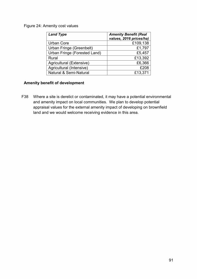
91

Figure 24: Amenity cost values

Land Type Amenity Benefit (Real values, 2016 prices/ha)

Urban Core £109,138 Urban Fringe (Greenbelt) £1,797 Urban Fringe (Forested Land) £5,457 Rural £13,392 Agricultural (Extensive) £6,366 Agricultural (Intensive) £208 Natural & Semi-Natural £13,371

Amenity benefit of development

F38 Where a site is derelict or contaminated, it may have a potential environmental

and amenity impact on local communities. We plan to develop potential appraisal values for the external amenity impact of developing on brownfield land and we would welcome receiving evidence in this area.

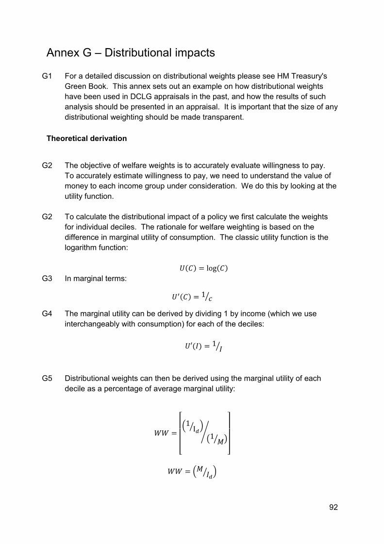
92

Annex G – Distributional impacts

G1 For a detailed discussion on distributional weights please see HM Treasury's Green Book. This annex sets out an example on how distributional weights have been used in DCLG appraisals in the past, and how the results of such analysis should be presented in an appraisal. It is important that the size of any distributional weighting should be made transparent.

Theoretical derivation

G2 The objective of welfare weights is to accurately evaluate willingness to pay.

To accurately estimate willingness to pay, we need to understand the value of money to each income group under consideration. We do this by looking at the utility function.

G2 To calculate the distributional impact of a policy we first calculate the weights

for individual deciles. The rationale for welfare weighting is based on the difference in marginal utility of consumption. The classic utility function is the logarithm function:

𝑈(𝐶) = log(𝐶) G3 In marginal terms:

𝑈′(𝐶) = 1 𝑐�

G4 The marginal utility can be derived by dividing 1 by income (which we use interchangeably with consumption) for each of the deciles:

𝑈′(𝐼) = 1

𝐼�

G5 Distributional weights can then be derived using the marginal utility of each decile as a percentage of average marginal utility:

𝑊𝑊 =

⎣⎢⎢⎢⎡�1

I𝑑� �

�1𝑀� �

�

⎦⎥⎥⎥⎤

𝑊𝑊 = �𝑀 𝐼𝑑� �

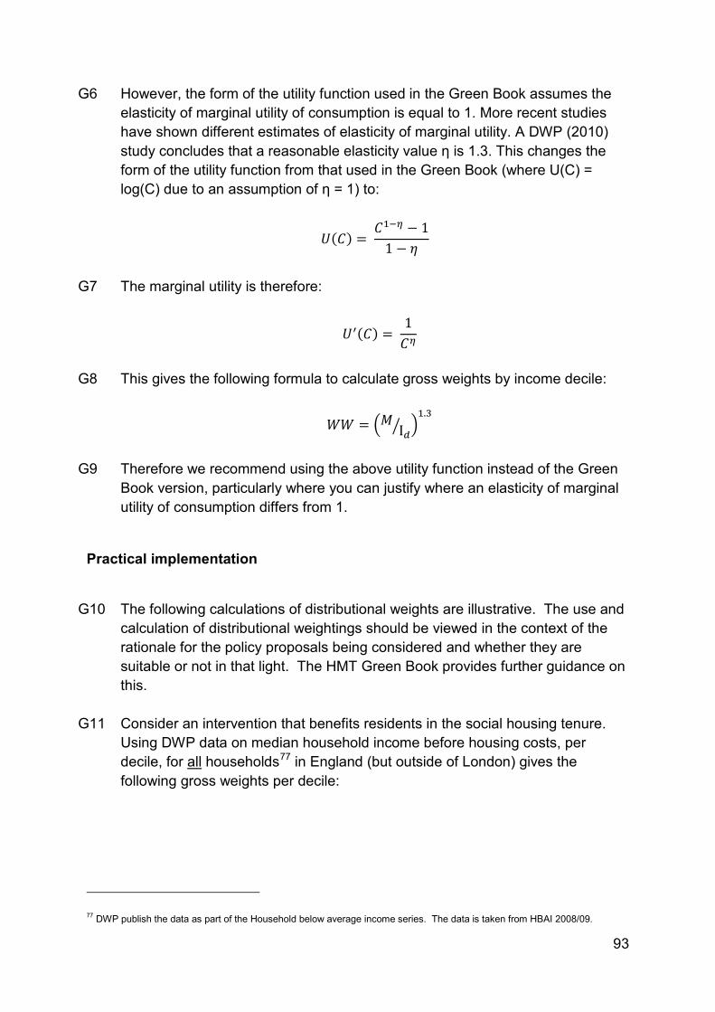
93

G6 However, the form of the utility function used in the Green Book assumes the elasticity of marginal utility of consumption is equal to 1. More recent studies have shown different estimates of elasticity of marginal utility. A DWP (2010) study concludes that a reasonable elasticity value η is 1.3. This changes the form of the utility function from that used in the Green Book (where U(C) = log(C) due to an assumption of η = 1) to:

𝑈(𝐶) = 𝐶1−𝜂 − 1

1 − 𝜂

G7 The marginal utility is therefore:

𝑈′(𝐶) = 1𝐶𝜂

G8 This gives the following formula to calculate gross weights by income decile:

𝑊𝑊 = �𝑀 I𝑑� �1.3

G9 Therefore we recommend using the above utility function instead of the Green

Book version, particularly where you can justify where an elasticity of marginal utility of consumption differs from 1.

Practical implementation

G10 The following calculations of distributional weights are illustrative. The use and

calculation of distributional weightings should be viewed in the context of the rationale for the policy proposals being considered and whether they are suitable or not in that light. The HMT Green Book provides further guidance on this.

G11 Consider an intervention that benefits residents in the social housing tenure.

Using DWP data on median household income before housing costs, per decile, for all households77 in England (but outside of London) gives the following gross weights per decile:

77 DWP publish the data as part of the Household below average income series. The data is taken from HBAI 2008/09.

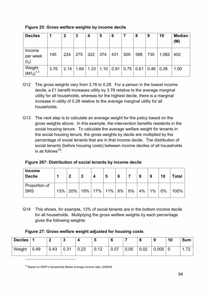
94

Figure 25: Gross welfare weights by income decile

Deciles 1 2 3 4 5 6 7 8 9 10 Median (M)

Income per week (Id)

145 224 275 322 374 431 500 588 730 1,082 402

Weight (M/Id)1.3

3.76 2.14 1.64 1.33 1.10 0.91 0.75 0.61 0.46 0.28 1.00

G12 The gross weights vary from 3.76 to 0.28. For a person in the lowest income

decile, a £1 benefit increases utility by 3.76 relative to the average marginal utility for all households, whereas for the highest decile, there is a marginal increase in utility of 0.28 relative to the average marginal utility for all households.

G13 The next step is to calculate an average weight for the policy based on the

gross weights above. In this example, the intervention benefits residents in the social housing tenure. To calculate the average welfare weight for tenants in the social housing tenure, the gross weights by decile are multiplied by the percentage of social tenants that are in that income decile. The distribution of social tenants (before housing costs) between income deciles of all households is as follows78:

Figure 267: Distribution of social tenants by income decile

Income Decile 1 2 3 4 5 6 7 8 9 10 Total

Proportion of SRS 13% 20% 19% 17% 11% 8% 6% 4% 1% 0% 100%

G14 This shows, for example, 13% of social tenants are in the bottom income decile for all households. Multiplying the gross welfare weights by each percentage gives the following weights:

Figure 27: Gross welfare weight adjusted for housing costs

Deciles 1 2 3 4 5 6 7 8 9 10 Sum

Weight 0.49 0.43 0.31 0.23 0.12 0.07 0.05 0.02 0.005 0 1.72

78 Based on DWP’s Households Below Average Income data, 2008/09

95

G15 Summing across all the weights gives an average weight for all social

households of 1.72.

G16 We then calculate welfare weights net of the cost to taxpayers (to reflect the negative marginal utility for households arising from paying taxes and other revenue raising activities). So we subtract the £1 of transfer from the £1.72 benefit, leaving only £0.72 of pure welfare gain. In other words, spending £1 on a social housing tenant has an additional welfare equity effect of 72 pence on top of the direct £1 benefit which they receive from the spending.

Practical example

G17 The current (2003) version of the Green Book recommends multiplying benefits

by a welfare weight. For business cases relating to affordable housing (and thus, social tenants), the rent subsidy that tenants would receive has been calculated as the difference between average market rents and the affordable rent post-intervention. In effect, this calculates the amount of additional money these tenants would have in their pocket compared to if they had to pay a market rent.

G18 In 2014, the average market rent was £595 per month, whereas the average

affordable rent was £513, the difference therefore being £82 per month. The difference is funded by direct government subsidy. If no welfare weights were applied, only the difference of £82 would be included in the NPPV or BCR.

G19 However, assuming that the subsidy is distributed in accordance with the

existing distribution of income of social tenants, welfare weights could be used to calculate the additional distributional benefit of the changes. This means multiplying £82 by 0.72, which gives an additional £56 benefit per month per tenant.

96

Bibliography Bramley, G., Fitzpatrick, S. et al. (2015), Hard Edges – Mapping severe and multiple disadvantage. LankellyChase Foundation.

BRE (2015), Briefing paper: The cost of poor housing to the NHS.

Bretherton, J & Pleace, N. (2015) 'Housing First in England', Centre for Housing Policy, University of York.

Cabinet Office (2014), Fair Chance Fund – will improving outcomes make savings across the public sector?

The Department for Transport (2014), Transport Appraisal Guidance: Webtag.

Eftec & Entec (2001), Valuing the external benefits of undeveloped land: main document.

DCLG (2015), Cost of rough sleeping. Working paper.

DCLG/CapGemini (2009), Research into the financial benefits of the Supporting People programme.

Department of Health (2010), Healthcare for single homeless people. Office of the Chief Analyst.

Department for Work and Pensions (2010), The Department for Work and Pensions Social Cost-Benefit Analysis Framework, Working Paper No 86

De Sousa C (2002), 'Measuring the public costs and benefits of brownfield versus greenfield development in the Greater Toronto area', Environment and Planning B: Planning and Design 2002, volume 29.

European Observatory on Homelessness (2013), 'The Costs of Homelessness in Europe – An Assessment of the Current Evidence Base', Comparative Studies on Homelessness No. 3.

FTI Consulting & Compass Lexecon (2014), Evaluation of the MEAM pilots.

Graham D, Gibbons S, Martin R (2009), 'Transport Investment and the Distance Decay of Agglomeration Benefits', Centre for Transport Studies.

HM Treasury (2013), ‘Public Sector Business Cases’, Green Book Supplementary Guidance on Delivering Public Value from Spending Proposals.

HM Treasury (2003), The Green Book: Appraisal and Evaluation in Central Government.

97

Larimer, M.E., Malone, D.K., Garner, M.D. et al. (2009), 'Health care and public service use and costs before and after provision of housing for chronically homeless persons with severe alcohol problems', JAMA, 301(13): 1349-1357.

New Policy Institute (2003), How Many, How Much? Single homelessness and the question of numbers and cost, Crisis.

Rossi-Hansberg and Sarte (2012), Economics of Housing Externalities.

Rossi-Hansberg, Sarte and Owens (2010), 'Housing Externalities', Journal of Political Economy, vol. 118, no. 3.

Venables, A., Overman, H., Laird, J. (2014), Transport investment and economic performance: Implications for project appraisal.

Zaretzky, K., Flatau, P. & Brady, M. (2008), 'What is the (Net) Cost to Government of Homelessness Programmes?,' Australian Journal of Social Issues, Vol.43 No.2.