1 

The date of interbreeding between Neandertals and modern humans

Sriram Sankararaman1,2,*, Nick Patterson2, Heng Li2, Svante Pääbo3* & David Reich1,2*

1Department of Genetics, Harvard Medical School, Boston, MA, 02115 USA; 2Broad Institute of MIT and Harvard, Cambridge, MA, 02142 USA;

3Department of Evolutionary Genetics, Max Planck Institute for Evolutionary Anthropology, Leipzig, D-04103 Germany.

* Correspondence to: Sriram Sankaramanan (sankaramaran@genetics.med.harvard.edu), Svante

Pääbo (paabo@eva.mpg.de) or David Reich (reich@genetics.med.harvard.edu)

Abstract

Comparisons of DNA sequences between Neandertals and present-day humans have

shown that Neandertals share more genetic variants with non-Africans than with

Africans. This could be due to interbreeding between Neandertals and modern

humans when the two groups met subsequent to the emergence of modern humans

outside Africa. However, it could also be due to population structure that antedates

the origin of Neandertal ancestors in Africa. We measure the extent of linkage

disequilibrium (LD) in the genomes of present-day Europeans and find that the last

gene flow from Neandertals (or their relatives) into Europeans likely occurred

37,000-86,000 years before the present (BP), and most likely 47,000-65,000 years

ago. This supports the recent interbreeding hypothesis, and suggests that

interbreeding may have occurred when modern humans carrying Upper Paleolithic

technologies encountered Neandertals as they expanded out of Africa. arX

iv:1

208.

2238

v1 [

q-bi

o.PE

] 1

0 A

ug 2

012

  2 

Author Summary

One of the key discoveries from the analysis of the Neandertal genome is that

Neandertals share more genetic variants with non-Africans than with

Africans. This observation is consistent with two hypotheses: interbreeding

between Neandertals and modern humans after modern humans emerged out

of African or population structure in the ancestors of Neandertals and

modern humans. These hypotheses make different predictions about the date

of last gene exchange between the ancestors of Neandertals and modern non-

Africans. We estimate this date by measuring the extent of linkage

disequilibrium (LD) in the genomes of present-day Europeans and find that

the last gene flow from Neandertals into Europeans likely occurred 37,000-

86,000 years before the present (BP), and most likely 47,000-65,000 years ago.

This supports the recent interbreeding hypothesis, and suggests that

interbreeding occurred when modern humans carrying Upper Paleolithic

technologies encountered Neandertals as they expanded out of Africa.

  3 

Introduction

A much-debated question in human evolution is the relationship between modern humans

and Neandertals. Modern humans appear in the African fossil record about 200,000 years

ago. Morphological traits typical of Neandertals appear in the European fossil record

about 400,000 years ago [1] and disappear about 30,000 year ago. They lived in Europe

and western Asia with a range that extended as far east as Siberia [2] and as far south as

the middle East. The overlap of Neandertals and modern humans in space and time

suggests the possibility of interbreeding. Evidence, both for [3] and against interbreeding

[4], have been put forth based on the analysis of modern human DNA. Although

mitochondrial DNA from multiple Neandertals has shown that Neandertals fall outside

the range of modern human variation [5,6,7,8,9,10], low-levels of gene flow cannot be

excluded [10,11,12].

Analysis of the draft sequence of the Neandertal genome revealed that the Neandertal

genome shares more alleles with non-African than with sub-Saharan African genomes

[13]. One hypothesis that could explain this observation is a history of gene flow from

Neandertals into modern humans, presumably when they encountered each other in

Europe and the Middle East [13] (Figure 1). An alternative hypothesis is that the findings

are explained by ancient population structure in Africa [13,14,15,16], whereby the

population ancestral to Neandertal and modern human ancestors was subdivided. If this

substructure persisted until modern humans carrying Upper Paleolithic technologies

expanded out of Africa so that the modern human population that migrated was

genetically closer to Neandertals, people outside Africa today would share more genetic

variants with Neandertals that people in sub-Saharan Africa [13,14,15] (Figure 1).

Ancient substructure in Africa is a plausible alternative to the hypothesis of recent gene

flow. Today, sub-Saharan Africans harbor deep lineages that are consistent with a highly-

structured ancestral population [17,18,19,20,21,22,23,24,25,26,27]. Evidence for ancient

structure in Africa has also been offered based on the substantial diversity in neurocranial

geometry amongst early modern humans [28]. Thus, it is important to test formally

whether substructure could explain the genetic evidence for Neandertals being more

closely related to non-Africans than to Africans.

  4 

A direct way to distinguish the hypothesis of recent gene flow from the hypothesis of

ancient substructure is to infer the date for when the ancestors of Neandertals and a

modern non-African population last exchanged genes. In the recent gene flow scenario,

the date is not expected to be much older than 100,000 years ago, corresponding to the

time of the earliest documented modern humans outside of Africa[29]. In the ancient

substructure scenario, the date of last common ancestry is expected to be at least 230,000

years ago, since Neandertals must have separated from modern humans by that time

based on when the first definitive Neandertals appear in the fossil record of Europe[1].

In present-day human populations, the extent of LD between two single nucleotide

polymorphisms (SNPs) shared with Neandertals can be the result of two phenomena.

First, there is “non-admixture LD” [30] whose extent reflects stretches of DNA inherited

from the ancestral population of Neandertals and modern humans as well as LD that has

arisen due to bottlenecks and genetic drift in modern humans since they separated from

Neandertals. Second, if gene flow from Neandertals into modern humans occurred, there

is “admixture LD”[30], which will reflect stretches of genetic material inherited by

modern humans through interbreeding with Neandertals. The extent of LD between

single nucleotide polymorphisms (SNPs) shared with Neandertals will thus reflect, at

least in part, the time since Neandertals or their ancestors and modern humans or their

ancestors last exchanged genes with each other.

The strategy of using LD to estimate dates of gene flow events has been previously been

explored by several groups [31,32,33,34,35]. Our methodology is conceptually similar to

the methodology developed by Moorjani et al., but is dealing with a more challenging

technical problem since the methodology developed by Moorjani et al. is adapted for

relatively recent admixtures. In recently admixed populations that have not experienced

recent bottlenecks, admixture LD extends over size scales at which non-admixture LD

makes a negligible contribution. Thus, one can infer the time of gene flow based on inter-

marker spacings that are larger than the scale of non-admixture LD. For older admixtures

however (such as may have occurred in the case of Neandertals), non-admixture LD

occurs almost at the same size scale as admixture LD. To account for this, we study pairs

of markers that are very close to each other, but ascertain them in a way that greatly

  5 

minimizes the signals of non-admixture LD while enhancing the signals of admixture

LD. Thus, unlike in the case of recent admixtures, non-admixture LD could bias an

admixture date obtained using our methods; however, we show using simulations of a

very wide set of demographic scenarios that that our marker ascertainment procedure

makes the bias so small that our inferences are qualitatively unaffected.

Our methodology is based on the idea that if two alleles, a genetic distance x (expected

number of crossover recombination events per meiosis) apart, arose on the Neandertal

lineage and introgressed into modern humans at time tGF, the probability that these alleles

have not been broken up by recombination since gene flow is proportional to e-ttGFx. The

LD across introgressed pairs of alleles is expected to decay exponentially with genetic

distance. The rate of decay is informative of the time of gene flow and is robust to

demographic events (Appendix A, Supporting Information S1). In practice, we need to

ascertain SNPs that, assuming recent gene flow occurred, are likely to have arisen on the

Neandertal lineage and introgressed into modern humans. We choose a particular

ascertainment scheme and show, using simulations of a number of demographic models,

that the exponential decay of LD across pairs of ascertained SNPs provides accurate

estimates of the time of gene flow. A second potential source of bias in estimating ancient

dates arises from uncertainties in the genetic map. We develop a correction for this bias

and show that this correction yields accurate dates in the presence of uncertainties in the

genetic map. Combining these various strategies, we are able to obtain accurate

estimates of the date of last exchange of genes between Neandertals and modern humans

(also see Discussion). This date shows that recent gene flow between Neandertals and

modern humans occurred but does not exclude that ancient substructure in Africa also

contributes to the LD observed.

Results

To study how LD decays with the distance in the genome, we computed the average

value, , of the measure of linkage disequilibrium D (the excess rate of occurrence of

derived alleles at two SNPs compared with the expectation if they were independent[36])

between pairs of SNPs binned by genetic distance x (see Methods). Immediately after the

time of last gene flow between Neandertal (or their relatives) and human ancestors, long

  6 

range LD is generated, and it is then expected to decay at a constant rate per generation as

recombination breaks down the segments shared with Neandertals. Thus, in the absence

of new LD-generating events (discussed further below), the statistic across pairs of

introgressed alleles is expected to have an exponential decay with genetic distance, and

the genetic extent of the decay can thus be interpreted in terms of the time of last shared

ancestry between Neandertals (or their relatives) and modern humans (Section S1 and

Appendix A in Supporting Information S1).

To amplify the signal of admixture LD relative to non-admixture LD, we restricted our

analysis to SNPs where the “derived” allele (the one that has arisen as a new mutation as

determined by comparison to chimpanzee) is found in Neandertals and occurs in the

tested population at a frequency of <10%. The justification for this frequency threshold

is two-fold. First, the signal of Neandertals being more closely related to non-Africans

than to Africans is substantially enriched at SNPs below this threshold (Section S1 in

Supporting Information S1). Second, under the model of recent gene flow, such SNPs

have an increased probability of having arisen due to mutations on the Neandertal

lineage; we estimate that about 30% of them will have arisen on the Neandertal lineage

under a model of history that we fitted to the data. This ascertainment enriches the class

of informative SNPs by a factor of ten (Section S1 in Supporting Information S1). Our

simulations show that restricting to this class of SNPs yields accurate estimates of the

time of gene flow for a wide range of demographic histories consistent with patterns of

human variation (Section S2 in Supporting Information S1).

To assess how useful this statistic is for measuring admixture LD, we performed

coalescent simulations of 100 regions of a million base pairs each, for a range of

demographic histories chosen to be plausible for Neandertals, West Africans and non-

Africans (these histories were constrained by the observed population differentiation

between west Africans and Europeans as measured by their FST and the quantitative

extent to which Neandertals share more derived alleles with Europeans than with

Africans). The simulation results, which we discuss at length in Section S2 of Supporting

Information S1, and summarize in Table 2, show that we obtain accurate and relatively

unbiased estimates of the number of generations since admixture (never more than 15%

  7 

from the true value) for (1) constant-sized population scenarios, (2) demographic models

that include population bottlenecks as well as more recent admixture after the gene flow,

(3) hybrid models of ancient structure and recent gene flow, and (4) mutation rates that

differ by a factor of 5 from what we use in our main simulations ( see Fig 2). Two other

SNP ascertainment schemes yield qualitatively consistent findings but the ascertainment

we used provides the most accurate estimates under the range of demographic models

considered (Section S5 of Supporting Information S1 and Table 2). The simulations also

show that in the absence of gene flow (including in the scenario of ancient subdivision),

the dates obtained are always at least 5,000 generations for scenarios of demographic

history that match the constraints of real human data. Thus, an empirical estimate of a

date much less than 5,000 generations likely reflects real gene flow.

We applied our statistic to data from Pilot 1 of the 1000 Genomes Project, which

discovered polymorphisms in 59 West Africans, 60 European Americans, and 60 East

Asians (Han Chinese and Japanese from Tokyo) [37]. We binned pairs of SNPs by the

genetic distance between them using the deCODE genetic map. We considered all pairs

of SNPs that are at most 1cM apart. We computed the average LD over all pairs of SNPs

in each bin and fit an exponential curve to the decay of LD (from 0.02-1cM in 0.001cM

increments).

Figure 3 shows the extent of LD for pairs of SNPs where both SNPs have a derived allele

frequency <10%. This figure shows that the extent of LD is larger in Europeans and East

Asians than in West Africans, both when the Neandertal genome carries the derived and

when it carries the ancestral allele. Empirical features of these LD decay curves show

that, alleles derived in the Neandertal genome, the pattern in Europeans and East Asians

is reflecting “admixture LD”. LD in West Africans is less extensive when Neandertals

carry the derived allele than when they carry the ancestral allele, while the reverse is seen

in Eurasians. To understand this, we note that in the absence of gene flow, polymorphic

sites where Neandertals carry the derived allele must have arisen from mutations that

occurred prior to Neandertal-human divergence so that they are old and recombination

will have had a lot of time to break down the LD, while sites where Neandertals carry the

ancestral allele mutations will include mutations that have arisen since the Neandertal-

  8 

human split and thus LD will be expected to be more extensive, exactly as is seen in West

Africans. In contrast, if gene flow occurred, then LD can be greater at sites where

Neandertals carry the derived allele as is observed in Europeans and East Asians. This

signal persists when we stratify the LD decay curves by the frequency of the ascertained

SNPs (Figure S8 in Supporting Information S1). Thus the scale of the LD at these sites

must be conveying information about the date of gene flow.

A concern in interpreting the extent of LD in terms of a date is that all available genetic

maps (which specify the probability of recombination per generation between all pairs of

SNPs) are likely to be inaccurate at the scale of tens of kilobases that is relevant to our

analysis. We confirmed that errors in genetic maps can bias LD-based date estimates by

simulating a gene flow event 2,000 generations ago using a model in which

recombination was localized to hot spots [38] but where the data were analyzed assuming

a genetic map that assumed homogeneous recombination rates across the genome. This

led to a date of 1,597 generations since admixture. We developed a statistical model of

the random errors that relate the true and observed genetic maps (see Methods). The

precision of the map is modeled using a scalar parameter α. A unit interval of the

observed genetic map corresponds to an interval in the true map of expected unit length

and variance 1/α. To validate this error model, we estimated the map error in these

simulations (α) by comparing the true and the observed genetic maps. Theoretical

arguments (Section S3 in Supporting Information S1) show that we can obtain a

corrected date (tGF) from the uncorrected date in generations (λ) using the equation tGF =

α(eλ/α - 1). We applied this correction to obtain a date of 1,926 generations. While this

error model appears to provide an adequate description of random errors in a genetic

map, it does not account for systematic biases.

To apply this statistical correction to real data, we estimated the error rate α in the genetic

map by comparing the genomic distribution of a set of cross-over events from 728

meioses previously detected in a European American Hutterite pedigree [39] to what

would be expected if the map were perfect. Unfortunately, the map that we would ideally

want to use for estimating the date of Neandertal admixture is not the genetic map that

applies to Hutterites today, but the time-averaged genetic map that applied between the

  9 

present and the date of gene flow. Obviously, such a map is not available, but we

hypothesize that by performing our analyses using a genetic map that is built from

samples more closely related to the Hutterite pedigree than the map that we would like to

analyze (the deCODE pedigree map built in Icelanders) as well as a genetic map that

averages over too long a period of time (the European LD Map, which measures

recombination over approximately five hundred thousand years), we can obtain some

sense of the robustness of our inferences to uncertainties in how the European genetic

map has changed over time.

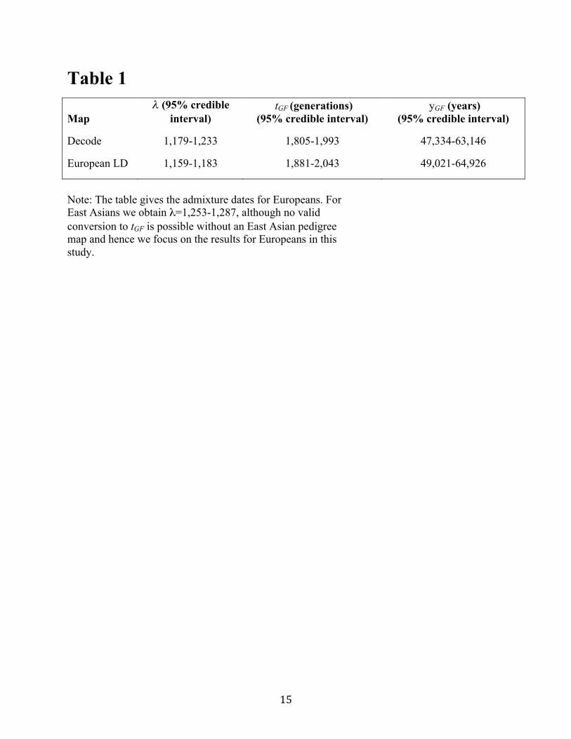
Table 1 shows the estimates of λ, α and tGF in Europeans obtained using the two genetic

maps. The estimates of tGF are in 1,805-2,043 for both the deCODE and European LD

maps. We also estimated λ in East Asians using the “East Asian LD map”. We find that λ

in East Asians based on the East Asian LD map is 1,253-1,287, similar to the 1,159-1,183

in Europeans based on the European LD map, although the similarity of the these

numbers does not prove the Neandertal genetic material in Europeans and East Asians

derives from the same ancestral gene flow event. While a shared ancestral gene flow

event is plausible, the gene flow events could in principle have occurred in different

places at around the same time [40]. We also cannot reliably estimate the recombination

rate correction factor α for the East Asian map because we do not have access to cross-

over events in an East Asian pedigree, and hence we do not present an estimate of tGF in

East Asians and focus on Europeans in the rest of this paper.

To convert the date estimates in generations to date estimates in years, we use an average

generation interval which has been estimated to be 29 in diverse modern hunter gatherer

societies as well as in developing and industrialized nation states [41]. We assume a

uniform prior probability distribution of generation times between 25 and 33 years per

generation for the true value of this quantity and integrate this with the uncertainty of λ

and α, and obtain an estimate of last gene exchange between Neandertals and European

ancestors of 47,334-63,146 years for the deCODE map, and 49,021-64,926 years for the

European LD Map (95% credible intervals). Taking the conservative union of these

ranges, we obtain 47,000-65,000 years BP. In our simulations of ascertainment strategy,

we found demographic models that can produce biases in the date estimates that could be

  10 

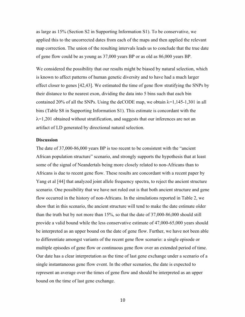
as large as 15% (Section S2 in Supporting Information S1). To be conservative, we

applied this to the uncorrected dates from each of the maps and then applied the relevant

map correction. The union of the resulting intervals leads us to conclude that the true date

of gene flow could be as young as 37,000 years BP or as old as 86,000 years BP.

We considered the possibility that our results might be biased by natural selection, which

is known to affect patterns of human genetic diversity and to have had a much larger

effect closer to genes [42,43]. We estimated the time of gene flow stratifying the SNPs by

their distance to the nearest exon, dividing the data into 5 bins such that each bin

contained 20% of all the SNPs. Using the deCODE map, we obtain λ=1,145-1,301 in all

bins (Table S8 in Supporting Information S1). This estimate is concordant with the

λ=1,201 obtained without stratification, and suggests that our inferences are not an

artifact of LD generated by directional natural selection.

Discussion

The date of 37,000-86,000 years BP is too recent to be consistent with the “ancient

African population structure” scenario, and strongly supports the hypothesis that at least

some of the signal of Neandertals being more closely related to non-Africans than to

Africans is due to recent gene flow. These results are concordant with a recent paper by

Yang et al [44] that analyzed joint allele frequency spectra, to reject the ancient structure

scenario. One possibility that we have not ruled out is that both ancient structure and gene

flow occurred in the history of non-Africans. In the simulations reported in Table 2, we

show that in this scenario, the ancient structure will tend to make the date estimate older

than the truth but by not more than 15%, so that the date of 37,000-86,000 should still

provide a valid bound while the less conservative estimate of 47,000-65,000 years should

be interpreted as an upper bound on the date of gene flow. Further, we have not been able

to differentiate amongst variants of the recent gene flow scenario: a single episode or

multiple episodes of gene flow or continuous gene flow over an extended period of time.

Our date has a clear interpretation as the time of last gene exchange under a scenario of a

single instantaneous gene flow event. In the other scenarios, the date is expected to

represent an average over the times of gene flow and should be interpreted as an upper

bound on the time of last gene exchange.

  11 

While recent gene flow from Neandertals into the ancestors of modern non-Africans is a

parsimonious model that is consistent with our results, our analysis cannot reject the

possibility that gene flow did not involve Neandertals themselves, but instead populations

that were more closely related to Neandertals than any extant populations are today.

Thus, the date should be interpreted as the last period of time when genetic material from

Neandertals or an archaic population related to Neandertals entered modern humans.

Genetic analyses by themselves offer no indication of where gene flow may have

occurred geographically. However, the date in conjunction with the archaeological

evidence suggests that the two populations likely met somewhere in Western Eurasia. An

attractive hypothesis is the Middle East, where archaeological and fossil evidence

indicate that modern humans appeared before 100,000 years ago (as reflected by the

modern human remains in Skhul and Qafzeh caves), Neandertals expanded around

70,000 years ago (as reflected for example by the Neandertal remains at Tabun Cave),

and modern humans re-appeared around 50,000 years ago [29]. Our genetic date

estimates, which have a mostly likely range of 47,000-65,000 years ago (and are

confidently below 86,000 years ago), are too recent to be consistent with the appearance

of the first fossil evidence of modern humans outside of Africa—that is, our date makes it

unlikely that the Neandertal genetic material in modern humans today could arise

exclusively due to the gene flow involving the Skhul/Qafzeh modern humans—and

instead point to gene flow in a more recent period, possibly when modern humans

carrying Upper Paleolithic technologies expanded out of Africa.

  12 

Methods

Linkage disequilibrium statistic: Our procedure computes a statistic based on the LD

observed between pairs of SNPs. For all pairs of ascertained SNPs at a genetic distance x,

we compute the statistic:

Here S(x) denotes the set of all pairs of ascertained SNPs that are at a genetic distance x,

and D(i,j) denotes the classic signed measure of linkage disequilibrium, D, at the SNPs i,

j. The sign of D(i,j) is determined by computing D using the derived alleles (defined

relative to the chimpanzee base) at SNPs i and j. Under the gene flow scenario, we

expect the contribution of introgression to to have an exponential decay with rate

equal to the time of gene flow, provided the gene flow is more recent than the

Neandertal-modern human split (Section S1 and Appendix A of Supporting Information

S1).

We pick SNPs that contain a derived allele in Neandertal (defined relative to the

chimpanzee base) and are polymorphic in the target population with a derived allele

frequency <10%. Further details can be found in the Supporting Information, along with

simulations exploring the performance of the statistic and demonstrating its properties

under various demographic models and ascertainment schemes.

Preparation of 1000 Genomes Data and alignment to chimpanzee and Neandertal:

We used the 1000 Genomes Pilot 1 genotypes to estimate the LD decay. For each of the

panels that were chosen as the target population in our analysis, we restricted our analysis

to polymorphic SNPs. The SNPs were polarized relative to the chimpanzee base

(panTro2).

Computation of the LD statistic on 1000 Genomes Data: For the set of ascertained

SNPs, we compute as a function of the genetic distance x and fit an exponential

curve using ordinary least squares for x in the range of 0.02cM to 1cM in increments of

  13 

0.001 cM. The standard definition of D requires the availability of haplotypes. We

instead computed D(i,j) as the covariance between the genotypes observed at SNPs i and

j [45]. Simulations show that dates estimated using this definition of D on unphased

genotypes are very similar to the estimates obtained from haplotypes (Section S2.1.1 of

Supporting Information S1). We were concerned that the complicated method used in the

1000 Genomes Project for determining genotypes, which involved statistical imputation

and probabilistic calling of genotypes based on LD, might in some way be biasing our

inferences based on LD. Thus, we also computed D(i,j) for all pairs of SNPs that passed

our basic filters (SNPs that contain a derived allele in Neandertal and are polymorphic in

the target population with derived allele frequency <10% as estimated from the reads) by

computing LD directly from the reads, again using the SAMtools package[46], and obtain

qualitatively consistent results (Section S7 of Supporting Information S1). Further,

simulations to mimic the low power to call rare SNPs in the 1000 genomes data show that

our estimates are not sensitive to the deficit of rare alleles (Section S6 of Supporting

Information S1).

Correction for error in the genetic map: We have a genetic map G defined on m

markers. Each of the m-1 intervals is assigned a genetic distance gi, i=1,..m-1. These

genetic distances provide a prior distribution for the true underlying (unobserved) genetic

distances Zi. A reasonable prior on each Zi is then:

where α is a parameter that is specific to the map. This implies that the true genetic

distance Zi has mean gi and variance gi/α. Thus, large values of α correspond to a more

precise map. A motivation for the choice of the gamma prior over Zi is that this prior has

the key invariance property Z1+Z2∼Γ(α(g1+g2),α). Thus, α is a property of the map and

not of the specific markers used.

Given this prior on the true genetic distances, fitting an exponential function to pairs of

markers at a given observed genetic distance g involves integrating over the exponential

function evaluated at the true genetic distances given observed genetic distance g, that is:

  14 

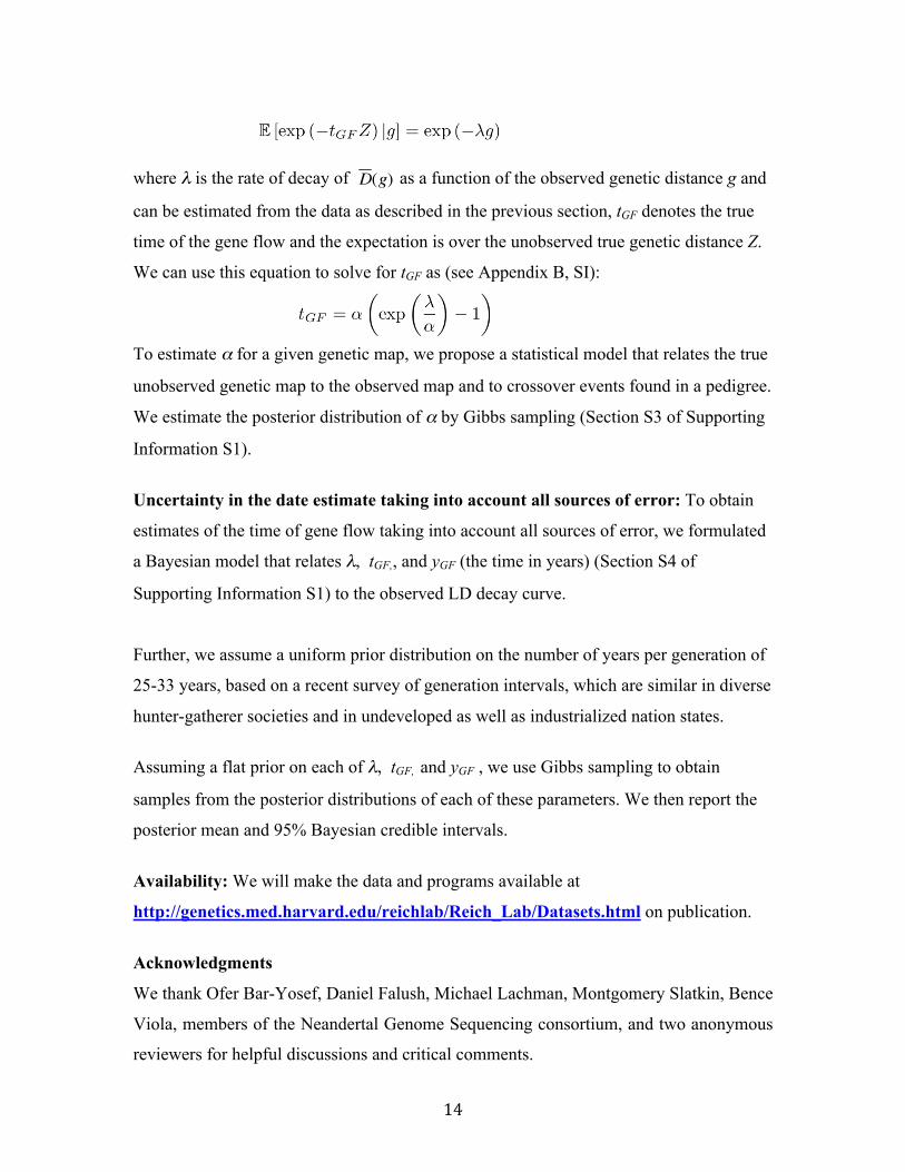
where λ is the rate of decay of as a function of the observed genetic distance g and

can be estimated from the data as described in the previous section, tGF denotes the true

time of the gene flow and the expectation is over the unobserved true genetic distance Z.

We can use this equation to solve for tGF as (see Appendix B, SI):

To estimate α for a given genetic map, we propose a statistical model that relates the true

unobserved genetic map to the observed map and to crossover events found in a pedigree.

We estimate the posterior distribution of α by Gibbs sampling (Section S3 of Supporting

Information S1).

Uncertainty in the date estimate taking into account all sources of error: To obtain

estimates of the time of gene flow taking into account all sources of error, we formulated

a Bayesian model that relates λ, tGF,, and yGF (the time in years) (Section S4 of

Supporting Information S1) to the observed LD decay curve.

Further, we assume a uniform prior distribution on the number of years per generation of

25-33 years, based on a recent survey of generation intervals, which are similar in diverse

hunter-gatherer societies and in undeveloped as well as industrialized nation states.

Assuming a flat prior on each of λ, tGF, and yGF , we use Gibbs sampling to obtain

samples from the posterior distributions of each of these parameters. We then report the

posterior mean and 95% Bayesian credible intervals.

Availability: We will make the data and programs available at

http://genetics.med.harvard.edu/reichlab/Reich_Lab/Datasets.html on publication.

Acknowledgments

We thank Ofer Bar-Yosef, Daniel Falush, Michael Lachman, Montgomery Slatkin, Bence

Viola, members of the Neandertal Genome Sequencing consortium, and two anonymous

reviewers for helpful discussions and critical comments.

  15 

Table 1

Map λ (95% credible

interval) tGF (generations)

(95% credible interval) yGF (years)

(95% credible interval)

Decode 1,179-1,233 1,805-1,993 47,334-63,146

European LD 1,159-1,183 1,881-2,043 49,021-64,926

Note: The table gives the admixture dates for Europeans. For East Asians we obtain λ=1,253-1,287, although no valid conversion to tGF is possible without an East Asian pedigree map and hence we focus on the results for Europeans in this study.

  16 

Table 2 Demography Fst (Y,E) D(Y,E,N) Ascertainment

0 Ascertainment

1 Ascertainment

2 No ancient structure and no gene flow NGF I 0.15 0 8847±126 7940±257 10206±280 NGF II 0.15 0 5800±164 7204±356 11702±451 Ancient structure AS I 0.15 0.045 10128±127 8162±107 8861±110 AS II 0.19 0.046 5070±397 6349±327 7570±433 Gene flow 2,000 generations ago RGF II 0.15 0.041 1987±48 1693±39 1960±43 RGF III 0.14 0.043 1776±87 1643±98 2272±102 RGF IV 0.15 0.04 2023±56 1751±36 1995±38 RGF V 0.07 0.04 2157±22 2094±22 2105±22 RGF VI 0.15 0.04 2102±36 1814±35 2029±38 Hybrid models of ancient structure and gene flow 2,000 generations ago HM I 0.18 0.03 2174±40 2057±30 2228±38 HM II 0.12 0.04 2226±39 2049±30 2100±30 HM III 0.13 0.04 2137±34 2040±29 2124±30 HM IV 0.18 0.06 2153±36 2038±34 2187±35 Gene flow 2,000 generations ago along with a varying mutation rate µ = 1×10-8/bp/gen. 0.11 0.04 2141±41 1847±35 1969±36 µ = 5×10-8/bp/gen. 0.11 0.04 2134±41 1833±29 1951±29 The table presents estimates of the time of gene flow for different demographic models and mutation rates as well as different ascertainments. The main classes of models are a) NGF: No gene flow in a randomly mating population; b) AS: Ancient structure, c) RGF : Recent (2,000 generation ago) gene flow from Neandertals (N) into European ancestors (E), d) HM: Hybrid models with ancient structure and recent gene flow and e) Mutation rates that are set to 1×10-

8/bp/generation and 5×10-8/bp/generation. The parameters of the models were chosen to match observed FST between Africans (Y) and Europeans (E) and to match the observed D-statistics of Africans and Europeans relative to Neandertal D(Y,E;N). In all models that involve recent gene flow, the time of gene flow was set to 2,000 generations. Our estimator of the time of gene flow provides accurate estimates of the time of gene flow for a wide range of demographic and mutational parameters. More details on the models and the ascertainments are in Fig 2, SI S2 and S5.

  17 

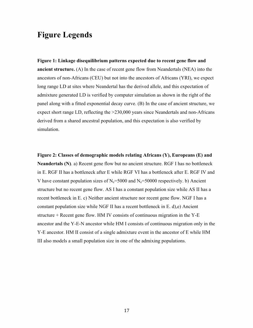
Figure Legends Figure 1: Linkage disequilibrium patterns expected due to recent gene flow and

ancient structure. (A) In the case of recent gene flow from Neandertals (NEA) into the

ancestors of non-Africans (CEU) but not into the ancestors of Africans (YRI), we expect

long range LD at sites where Neandertal has the derived allele, and this expectation of

admixture generated LD is verified by computer simulation as shown in the right of the

panel along with a fitted exponential decay curve. (B) In the case of ancient structure, we

expect short range LD, reflecting the >230,000 years since Neandertals and non-Africans

derived from a shared ancestral population, and this expectation is also verified by

simulation.

Figure 2: Classes of demographic models relating Africans (Y), Europeans (E) and

Neandertals (N). a) Recent gene flow but no ancient structure. RGF I has no bottleneck

in E. RGF II has a bottleneck after E while RGF VI has a bottleneck after E. RGF IV and

V have constant population sizes of Ne=5000 and Ne=50000 respectively. b) Ancient

structure but no recent gene flow. AS I has a constant population size while AS II has a

recent bottleneck in E. c) Neither ancient structure nor recent gene flow. NGF I has a

constant population size while NGF II has a recent bottleneck in E. d),e) Ancient

structure + Recent gene flow. HM IV consists of continuous migration in the Y-E

ancestor and the Y-E-N ancestor while HM I consists of continuous migration only in the

Y-E ancestor. HM II consist of a single admixture event in the ancestor of E while HM

III also models a small population size in one of the admixing populations.

 

 

 

 

  18 

Figure 3: Decay of LD for SNPs with minor allele frequency <10%. (A, B) Real data

for European Americans and East Asians shows longer range LD when the Neandertal

genome has the derived allele (left) than when it has the ancestral allele (right). This is as

expected due to gene flow from Neandertal, but is not expected in the absence of gene

flow. In other words, the fact that LD conditional on Neandertals having the derived

allele is longer than LD when Neandertal does not is proof that the pattern we are

observing among ascertained SNPs is reflecting the complex historical relationship

between non-African modern humans and Neandertals, the signal we care about here, and

not demographic events that solely involve the ancestors of non-Africans. The scale of

the LD decay (1/e drop of the fitted exponential curve) is shown in the top right of each

panel based on the deCODE genetic distance. (In Figure S8 of supporting Information

S1, we show that this signal persists when stratified into narrow allele frequency bins.)

(C) In West Africans the pattern is qualitatively different such that when Neandertal is

derived at both SNPs, LD decays more quickly than when Neandertal is ancestral at both

SNPs, as expected in the absence of gene flow (without gene flow, the derived allele is

always expected to be older so LD is expected to have had more time to break down).

 

 

 

 

 

 

 

 

 

 

 

 

 

  19 

List of Supplementary Figures Figure S1: The fraction of SNPs s where there is an excess of Neandertal derived alleles

n over Denisova derived alleles d as a function of the derived allele frequency in

Europeans.

Figure S2: Estimates of tGF as a function of true tGF for RGF I. We plot the mean and

twice the standard error of the estimates of tGF from 100 independent simulated datasets

using ascertainment 0. The estimates track the true tGF though the variance increases for

more ancient gene flow events.

Figure S3: Classes of demographic models. a) Recent gene flow but no ancient

structure. RGF I has no bottleneck in E. RGF II has a bottleneck after E while RGF VI

has a bottleneck after E. RGF IV and V have constant population sizes of Ne=5000 and

Ne=50000 respectively. b) Ancient structure but no recent gene flow. AS I has a constant

population size while AS II has a recent bottleneck in E. c) Neither ancient structure nor

recent gene flow. NGF I has a constant population size while NGF II has a recent

bottleneck in E. d),e) Ancient structure + Recent gene flow. HM IV consists of

continuous migration in the Y-E ancestor and the Y-E-N ancestor while HM I consists of

continuous migration only in the Y-E ancestor. HM II consist of a single admixture event

in the ancestor of E while HM III also models a small population size in one of the

admixing populations.

Figure S4: A graphical model for map error estimation. Each circle denotes a random

variable. Shaded circles indicate random variables that are observed. Plates

Figure S5: Estimates of tGF as a function of true tGF for Demography RGF I. We plot

the mean and twice standard error of the estimates of tGF from 100 independent simulated

datasets using ascertainment 1. The estimates track the true tGF though the variance

increases for more ancient gene flow events.

Figure S6: Impact of the ascertainment scheme on the estimates of tGF as a function

of tGF for Demography RGF I. We plot the mean and twice the standard error of the

estimates of tGF from 100 independent simulated datasets using ascertainment 2.

Figure S7: Estimates of tGF as a function of true tGF for RGF I when the SNPs were

filtered to mimic the 1000 genomes SNP calling process. We plot the mean and twice

the standard error of the estimates of tGF from 100 independent simulated datasets using

  20 

ascertainment 0. The estimates track the true tGF and are indistinguishable from estimates

obtained on the unfiltered dataset as seen in Figure S2.

Figure S8: Comparison of the LD decay conditioned on Neandertal derived alleles

and Neandertal ancestral alleles stratified by the derived allele frequency in CEU

(left) and YRI (right). In each panel, we compared the decay of LD for pairs of SNPs

ascertained in two ways. One set of SNPs were chosen so that Neandertal carried the

derived allele and where the number of derived alleles observed in the 1000 genomes

CEU individuals is a parameter x. The second set of SNPs were chosen so that

Neandertal carried only ancestral alleles and where the number of derived alleles

observed in 1000 genomes CEU is x. We varied x from 1 to 12 (corresponding to a

derived allele frequency of at most 10%). For each value of x, we estimated the extent of

the LD, i.e., the scale parameter of the fitted exponential curve. Standard errors were

estimated using a weighted block jackknife. Errorbars denote 1.96 times the standard

errors. The extent of LD decay shows a different pattern in CEU vs YRI. In YRI, the

extent of LD is similar across the two ascertainments to the limits of resolution although

the point estimates indicate that the LD tends to be greater at sites where Neandertal

carries the ancestral allele (8 out of 12). In CEU, on the other hand, the extent of LD is

significantly larger at sites where Neandertal carries the derived allele (the only exception

consists of singleton sites). Thus, the scale of LD at these sites must be conveying

information about the date of gene flow.

  21 

List of Supplementary Tables Table S1: Estimates of the time of gene flow for different demographies and

mutation rates.

Table S2: Correlation coefficient between times of gene flow estimated using

haplotype and genotype data vs the true time of gene flow.

Table S3: Estimates of time of gene flow as a function of the quality of the genetic

map. Data was simulated under a hotspot model of recombination. The observed genetic

map was obtained by perturbing the true genetic map at a 1 Mb scale and then

interpolating based on the physical positions of the markers. Smaller values of a indicate

larger perturbation. λ denotes the estimates obtained on the perturbed map. tGF denotes

the estimates obtained after correcting for the errors in the observed map. Results are

reported for two demographic models.

Table S4: Estimates of the precision of two Genetic maps.

Table S5: Estimates of time of gene flow for different demographies. For the

demographies that involve recent gene flow (RGF II, RGF III, RGF IV and RGF V), the

true time of gene flow is 2000 generations.

Table S6: Estimated time of the gene flow from Neandertals into Europeans (CEU)

and East Asians (CHB+JPT). λ refers to the uncorrected time in generations obtained

as described in Section S1. tGF refers to the time in generations obtained from λ by

integrating out the uncertainty in the genetic map as described in Section S3. yGF refers to

the time in years obtained from λ by integrating out the uncertainty in the genetic map

and the uncertainty in the number of years per generation (We are reporting the posterior

mean and 95% Bayesian credible intervals for each of these parameters). Estimates of the

time of gene flow were obtained for CEU using the Decode map and the CEU LD map.

Estimates for CHB+JPT were obtained using the CHB+JPT LD map (We do not have a

precise estimate of the uncertainty in this genetic map -- hence, we report only λ).

Table S7: Estimated time of the gene flow from Neandertals into Europeans (CEU)

under different ascertainment schemes. λ refers to the uncorrected time in generations

obtained as described in Section S1. Ascertainment 1 is shown to have a downward bias

in the presence of bottlenecks since the gene flow -- this may reflect the lower estimates

  22 

obtained here. The estimates using Ascertainment 2 closely match the estimates shown in

Table S6.

Table S8: Estimate of the time of gene flow stratified by distance to nearest exon

(each bin contain 20% of the 1000 genome SNPs). These estimates were obtained on

CEU using the Decode map. The results indicate that our estimates are not particularly

sensitive to the strength of directional selection, which has recently been shown to be a

widespread force in the genome.

References

 1. Hublin JJ (2009) Out of Africa: modern human origins special feature: the origin of 

Neandertals. Proceedings of the National Academy of Sciences of the United States of America 106: 16022‐16027. 

2. Krause J, Orlando L, Serre D, Viola B, Prufer K, et al. (2007) Neanderthals in central Asia and Siberia. Nature 449: 902‐904. 

3. Wall JD, Lohmueller KE, Plagnol V (2009) Detecting ancient admixture and estimating demographic parameters in multiple human populations. Molecular biology and evolution 26: 1823‐1827. 

4. Currat M, Excoffier L (2004) Modern humans did not admix with Neanderthals during their range expansion into Europe. PLoS biology 2: e421. 

5. Briggs AW, Good JM, Green RE, Krause J, Maricic T, et al. (2009) Targeted retrieval and analysis of five Neandertal mtDNA genomes. Science 325: 318‐321. 

6. Krings M (1997) Neandertal DNA sequences and the origin of modern humans. Cell 90: 19‐30. 

7. Orlando L (2006) Revisiting Neandertal diversity with a 100,000 year old mtDNA sequence. Curr Biol 16: R400‐R402. 

8. Ovchinnikov IV (2000) Molecular analysis of Neanderthal DNA from the northern Caucasus. Nature 404: 490‐493. 

9. Green RE, Malaspinas AS, Krause J, Briggs AW, Johnson PL, et al. (2008) A complete Neandertal mitochondrial genome sequence determined by high‐throughput sequencing. Cell 134: 416‐426. 

10. Serre D, Langaney A, Chech M, Teschler‐Nicola M, Paunovic M, et al. (2004) No evidence of Neandertal mtDNA contribution to early modern humans. PLoS biology 2: E57. 

  23 

11. Nordborg M (1998) On the probability of Neandertal ancestry. American journal of human genetics 63: 1237. 

12. Currat M, Excoffier L (2004) Modern humans did not admix with Neanderthals during their range expansion into Europe. PLoS Biol 2: e421. 

13. Green RE, Krause J, Briggs AW, Maricic T, Stenzel U, et al. (2010) A draft sequence of the Neandertal genome. Science 328: 710‐722. 

14. Reich D, Green RE, Kircher M, Krause J, Patterson N, et al. (2010) Genetic history of an archaic hominin group from Denisova Cave in Siberia. Nature 468: 1053‐1060. 

15. Durand EY, Patterson N, Reich D, Slatkin M (2011) Testing for ancient admixture between closely related populations. Molecular biology and evolution 28: 2239‐2252. 

16. Slatkin M, Pollack JL (2008) Subdivision in an ancestral species creates asymmetry in gene trees. Molecular biology and evolution 25: 2241‐2246. 

17. Tishkoff SA, Reed FA, Friedlaender FR, Ehret C, Ranciaro A, et al. (2009) The genetic structure and history of Africans and African Americans. Science 324: 1035‐1044. 

18. Garrigan D, Mobasher Z, Kingan SB, Wilder JA, Hammer MF (2005) Deep haplotype divergence and long‐range linkage disequilibrium at xp21.1 provide evidence that humans descend from a structured ancestral population. Genetics 170: 1849‐1856. 

19. Barreiro LB, Patin E, Neyrolles O, Cann HM, Gicquel B, et al. (2005) The heritage of pathogen pressures and ancient demography in the human innate‐immunity CD209/CD209L region. American journal of human genetics 77: 869‐886. 

20. Labuda D, Zietkiewicz E, Yotova V (2000) Archaic lineages in the history of modern humans. Genetics 156: 799‐808. 

21. Harris EE, Hey J (1999) X chromosome evidence for ancient human histories. Proceedings of the National Academy of Sciences of the United States of America 96: 3320‐3324. 

22. Harding RM, McVean G (2004) A structured ancestral population for the evolution of modern humans. Current opinion in genetics & development 14: 667‐674. 

23. Evans PD, Mekel‐Bobrov N, Vallender EJ, Hudson RR, Lahn BT (2006) Evidence that the adaptive allele of the brain size gene microcephalin introgressed into Homo sapiens from an archaic Homo lineage. Proceedings of the National Academy of Sciences of the United States of America 103: 18178‐18183. 

24. Hayakawa T, Aki I, Varki A, Satta Y, Takahata N (2006) Fixation of the human‐specific CMP‐N‐acetylneuraminic acid hydroxylase pseudogene and implications of haplotype diversity for human evolution. Genetics 172: 1139‐1146. 

25. Patin E, Barreiro LB, Sabeti PC, Austerlitz F, Luca F, et al. (2006) Deciphering the ancient and complex evolutionary history of human arylamine N‐acetyltransferase genes. American journal of human genetics 78: 423‐436. 

  24 

26. Kim HL, Satta Y (2008) Population genetic analysis of the N‐acylsphingosine amidohydrolase gene associated with mental activity in humans. Genetics 178: 1505‐1515. 

27. Garrigan D, Hammer MF (2006) Reconstructing human origins in the genomic era. Nature reviews Genetics 7: 669‐680. 

28. Gunz P, Bookstein FL, Mitteroecker P, Stadlmayr A, Seidler H, et al. (2009) Early modern human diversity suggests subdivided population structure and a complex out‐of‐Africa scenario. Proceedings of the National Academy of Sciences of the United States of America 106: 6094‐6098. 

29. Bar‐Yosef O (2011) In Casting the Net Wide, essays in memory of G Isaac (J Sept and D Pilbeam (ed)) Monographs of the American School of Prehistoric Research: Oxbow (in press)  

30. Falush D, Stephens M, Pritchard JK (2003) Inference of population structure using multilocus genotype data: linked loci and correlated allele frequencies. Genetics 164: 1567‐1587. 

31. Moorjani P, Patterson N, Hirschhorn JN, Keinan A, Hao L, et al. (2011) The history of African gene flow into Southern Europeans, Levantines, and Jews. PLoS genetics 7: e1001373. 

32. Machado CA, Kliman RM, Markert JA, Hey J (2002) Inferring the history of speciation from multilocus DNA sequence data: the case of Drosophila pseudoobscura and close relatives. Molecular biology and evolution 19: 472‐488. 

33. Price AL, Tandon A, Patterson N, Barnes KC, Rafaels N, et al. (2009) Sensitive detection of chromosomal segments of distinct ancestry in admixed populations. PLoS genetics 5: e1000519. 

34. Pugach I, Matveyev R, Wollstein A, Kayser M, Stoneking M (2011) Dating the age of admixture via wavelet transform analysis of genome‐wide data. Genome biology 12: R19. 

35. Plagnol V, Wall JD (2006) Possible ancestral structure in human populations. PLoS genetics 2: e105. 

36. R.C. Lewontin KK (1960) The evolutionary dynamics of complex polymorphisms. Evolution 14: 458‐472. 

37. The 1000 Genomes Project Consortium (2010) A map of human genome variation from population‐scale sequencing. Nature 467: 1061‐1073. 

38. Hellenthal G, Stephens M (2007) msHOT: modifying Hudson's ms simulator to incorporate crossover and gene conversion hotspots. Bioinformatics 23: 520‐521. 

39. Coop G, Wen X, Ober C, Pritchard JK, Przeworski M (2008) High‐resolution mapping of crossovers reveals extensive variation in fine‐scale recombination patterns among humans. Science 319: 1395‐1398. 

40. Currat M, Excoffier L (2011) Strong reproductive isolation between humans and Neanderthals inferred from observed patterns of introgression. Proceedings of the National Academy of Sciences of the United States of America 108: 15129‐15134. 

  25 

41. Fenner JN (2005) Cross‐cultural estimation of the human generation interval for use in genetics‐based population divergence studies. American journal of physical anthropology 128. 

42. Cai JJ, Macpherson JM, Sella G, Petrov DA (2009) Pervasive hitchhiking at coding and regulatory sites in humans. PLoS genetics 5: e1000336. 

43. McVicker G, Gordon D, Davis C, Green P (2009) Widespread genomic signatures of natural selection in hominid evolution. PLoS genetics 5: e1000471. 

44. Yang MA, Malaspinas AS, Durand EY, Slatkin M (2012) Ancient Structure in Africa Unlikely to Explain Neanderthal and Non‐African Genetic Similarity. Molecular biology and evolution. 

45. Weir B (2010) Genetic Data Analysis III: Sinauer Associates, Inc. 46. Li H, Ruan J, Durbin R (2008) Mapping short DNA sequencing reads and calling 

variants using mapping quality scores. Genome research 18: 1851‐1858. 

 

 

Supporting Information

August 13, 2012

Contents

S1 Statistic for dating 27S1.1 Statistic . . . . . . . . . . . . . . . . . . . . . . . . . . . . . . . . . . . . . . . . 27S1.2 Preparation of 1000 genomes data . . . . . . . . . . . . . . . . . . . . . . . . . . 28

S2 Simulation Results 29S2.1 Recent gene flow . . . . . . . . . . . . . . . . . . . . . . . . . . . . . . . . . . . 29S2.2 Ancient structure . . . . . . . . . . . . . . . . . . . . . . . . . . . . . . . . . . . 30S2.3 No gene flow . . . . . . . . . . . . . . . . . . . . . . . . . . . . . . . . . . . . . 30S2.4 Hybrid Models . . . . . . . . . . . . . . . . . . . . . . . . . . . . . . . . . . . . 31S2.5 Effect of the mutation rate . . . . . . . . . . . . . . . . . . . . . . . . . . . . . . 31

S3 Correcting for uncertainties in the genetic map 35S3.1 Correction . . . . . . . . . . . . . . . . . . . . . . . . . . . . . . . . . . . . . . . 35S3.2 Estimating α . . . . . . . . . . . . . . . . . . . . . . . . . . . . . . . . . . . . . 35S3.3 Inference . . . . . . . . . . . . . . . . . . . . . . . . . . . . . . . . . . . . . . . 37S3.4 Simulations . . . . . . . . . . . . . . . . . . . . . . . . . . . . . . . . . . . . . . 38S3.5 Results . . . . . . . . . . . . . . . . . . . . . . . . . . . . . . . . . . . . . . . . . 38

S4 Uncertainty in the date estimates 41

S5 Effect of ascertainment 42S5.1 Recent gene flow . . . . . . . . . . . . . . . . . . . . . . . . . . . . . . . . . . . 42S5.2 Ancient structure . . . . . . . . . . . . . . . . . . . . . . . . . . . . . . . . . . . 42S5.3 No gene flow . . . . . . . . . . . . . . . . . . . . . . . . . . . . . . . . . . . . . 42S5.4 Hybrid Models . . . . . . . . . . . . . . . . . . . . . . . . . . . . . . . . . . . . 42S5.5 Effect of the mutation rate . . . . . . . . . . . . . . . . . . . . . . . . . . . . . . 43S5.6 Application to 1000 genomes data . . . . . . . . . . . . . . . . . . . . . . . . . . 43

S6 Effect of the 1000 genomes SNP calling 46

S7 Effect of the 1000 genomes imputation 46

S8 Results 48

26

A Exponential decay of the statistic 51

B Proof of Equation 3 in Section S3 53

S1 Statistic for dating

A number of methods have been proposed to infer the demographic history and thus the populationdivergence times of closely-related species using multi-locus genotype data (see [1] and referencestherein). In this work, we seek to directly estimate the quantity of interest, i.e, the time of geneflow, by devising a statistic that is robust to demographic history. Our statistic is based on thepattern of LD decay due to admixture that we observe in a target population. The use of LD decayto test for gene flow is not entirely new ( [2, 3]). [2] devised an LD-based statistic to test thehypotheses of recent gene flow vs ancient shared variation. [3] devised a statistic that used thedecay of LD to obtain dates of recent gene flow events. The main challenge in our work is theneed to estimate extremely old gene flow dates (at least 10000 years BP) while dealing with theuncertainty in recombination rates.

S1.1 Statistic

Consider three populations Y RI, CEU and Neandertal, which we denote (Y,E,N). We want toestimate the date of last exchange of genes betweenN andE. In our demographic model, ancestorsof (Y,E) and N split tNH generations ago and Y and E split tY E generations ago. Assume thatthe gene flow event happened tGF generations ago with a fraction f of individuals from N . Wehave SNP data from several individuals in E and Y as well as low-coverage sequence data for N .

1. Pick SNPs according to an ascertainment scheme discussed below.

2. For all pairs of sites S(x) = {(i, j)} at genetic distance x, consider the statistic D(x) =∑(i,j)∈S(x)D(i,j)

|S(x)| . Here D(i, j) is the classic signed measure of LD that measures the excessrate of occurence of derived alleles at two SNPs compared to the expectation if they wereindependent [4].

3. If there was admixture and if our ascertainment picks pairs of SNPs that arose in Neandertaland introgressed (i.e., these SNPs were absent in E before gene flow), we expect D(x) tohave an exponential decay with rate given by the time of the admixture because D(x) is aconsistent estimator of the expected value of D at genetic distance x. We can show that,under a model where gene flow occurs at a time tGF and the truly introgressed alleles evolveaccording to Wright-Fisher diffusion, this expected value has an exponential decay with rategiven by tGF . Importantly, changes in population size do not affect the rate of decay althoughimperfections of the ascertainment scheme will affect this rate (see Appendix A for details).

We pick SNPs that are derived in N (at least one of the reads that maps to the SNP carriesthe derived allele), are polymorphic in E and have a derived allele frequency in E < 0.1. Thisascertainment enriches for SNPs that arose in the N lineage and introgressed into E (in addition toSNPs that are polymorphic in the NH ancestor and are segregating in the present-day population).We chose a cutoff of 0.10 based on an analysis that computes the excess of the number of siteswhere Neandertal carries the derived allele compared to the number of sites where Denisova carries

27

‐0.04

‐0.02

0

0.02

0.04

0.06

0.08

0.1

0.12

0.14

0.16

0‐0.1

0.1‐0.2

0.2‐0.3

0.3‐0.4

0.4‐0.5

0.5‐0.6

0.6‐0.7

0.7‐0.8

0.8‐0.9

0.9‐1

(n‐d)/s

DerivedallelefrequencyinEuropeans

Figure S 1: The fraction of SNPs s where there is an excess of Neandertal derived alleles n overDenisova derived alleles d as a function of the derived allele frequency in Europeans.

the derived allele stratified by the derived allele frequency in European populations ( (n−d)s

where sis the total number of polymorphic SNPs in Europeans). Given that Denisova and Neandertal aresister groups, we expect these numbers to be equal in the absence of gene flow. The magnitude ofthis excess is an estimate of the fraction of Neandertal introgressed alleles. Below a derived allelefrequency cutoff of 0.10 in Europeans, we see a significant enrichment of this statistic indicatingthat it is this part of the spectrum that is most informative for this analysis (see Figure S1).

To further explore the properties of this ascertainment scheme, we performed coalescent simu-lations under the RGF II model discussed in Section S2. We computed the fraction of ascertainedSNPs for which the lineages leading to the derived alleles in E coalesce with the lineage in Nbefore the split time of Neandertals and modern humans. This estimate provides us a lower boundon the number of SNPs that arose as mutations on the N lineage. We estimate that 30% of the as-certained SNPs arose as mutations in N leading to about 10-fold enrichment over the backgroundrate of introgressd SNPs which has been estimated at 1− 4% [5].

We also explored other ascertainment schemes in Section S5.For the set of ascertained SNPs, we compute D(x) as a function of the genetic distance x and

fit an exponential curve using ordinary least squares for x in the range of 0.02 cM to 1 cM in incre-ments of 10−3 cM. The standard definition of D requires haplotype frequencies. To compute Di,j

directly from genotype data, we estimated Di,j as the covariance between the genotypes observedat SNPs i and j [6]. We tested the validity of using genotype data on our simulations in Section S2.

S1.2 Preparation of 1000 genomes data

We used the individual genotypes that were called as part of the pilot 1 of the 1000 genomesproject [7] to estimate the LD decay. For each of the panels that were chosen as the target pop-ulation in our analysis, we restricted ourselves to polymorphic SNPs. The SNPs were polarizedrelative to the chimpanzee base(PanTro2).

28

S2 Simulation Results

To test the robustness of our statistic, we performed coalescent-based simulations under demo-graphic models that included recent gene flow, ancient structure and neither gene flow nor ancientstructure. The classes of demographic models are shown in Figure S2.5

S2.1 Recent gene flow

S2.1.1 RGF I

In our first set of simulations, we generated 100 independent 1 Mb regions under a simple demo-graphic model of gene flow from Neandertals into non-Africans. We set tNH = 10000, tY E =5000. All effective population sizes are 10000. The fraction of gene flow was set to 0.03. Wesimulated 100 Y and E haplotypes respectively and 1 N haplotype. While we simulate a singlehaploid Neandertal, the sequenced Neandertal genome consists of DNA from 3 individuals. Hence,the reads obtained belong to one of 6 chromosomes. However, our statistic relies on the Neander-tal genome sequence only to determine positions that carry a derived allele. We do not explicitlyleverage any pattern of LD from this data. In our simulations, two SNPs at which Neandertal car-ries the derived allele necessarily lie on a single chromosome and ,hence, are more likely to be inLD than two similar SNPs in the sequenced Neandertals. However, the genetic divergence acrossthe sequenced Vindija bones is quite low ( [8] estimates the average genetic divergence to be about6000 years) and so, we do not expect that this makes a big difference in practice.

We simulated 100 random datasets varying tGF from 0 to 4500. Figure S5 shows the estimatedtGF tracks the true tGF across the range of values of tGF . As tGF increases, the variance of ourestimates increases – a result of the increasing influence of the non-admixture LD on the signalsof ancient admixture LD. These results are encouraging given that our estimates were obtainedusing only about 1

30

th of the data that is available in practice. Further, to test the validity of theuse of genotype data, we also computed Pearson’s correlation r of estimates of tGF obtained fromgenotype data to estimates obtained from haplotype data and we estimated these correlations torange from 0.89 to 0.96 across different true tGF (see Table S2).

S2.1.2 RGF II

We assessed the effect of demographic changes since the gene flow on the estimates of the time ofgene flow. We used tNH = 10000, tY E = 2500 and tGF = 2000. The fraction of gene flow wasset to 0.03. We simulated a bottleneck at 1020 generations of duration 20 generations in whichthe effective population size decreased to 100. We also simulated a 120 generation bottleneckin Neandertals from 3120 generations in which the effective population size decreased to 100.These parameters were chosen so that Fst between Y and E and the D-statistic D(Y,E,N) matchthe observed values [5] (the value of the D-statistic D(Y,E,N) depends on the probability of aEuropean lineage entering the Neandertal population and coalescing with a Neandertal lineagebefore tNH and could have been fit to the data by also adjusting f or tNH) . We see in Table S 1that the estimated time remains unbiased.

29

S2.1.3 RGF III

We used a version of the demography used in [9] modified to match the Fst between Y and E andthe D-statistics D(Y,E,N). In this setup, tNH = 14400, tY E = 2400 ,tGF = 2000, f = 0.03.Effective population sizes are 10000 in the E, Y E ancestor, NH ancestor, and 106 in modernday Y . Modern day Y underwent exponential growth from a size of 10000 over the last 1000generations. Y and E exchange genes after the split at a rate of 150 per generation. E underwenta bottleneck starting at 1440 generations that lasted 40 generations and had an effective populationsize of 320 during the bottleneck. We again generated 100 independent 1 Mb regions under thisdemography.

Table S1 shows that the estimates now have a small downward bias.

S2.1.4 RGF IV,V, VI

This is the same as RGF II but instead of a bottleneck we simulated a constant Ne in population Esince gene flow. Ne was set to 5000 (RGF IV) and 50000 (RGF V). RGF VI places the bottleneckbefore the gene flow ( the bottlenck begins at 2220 generations, has a duration of 20 generationsin which the effective population size decreased to 100). Table S1 shows that the estimates remainaccurate in these settings.

S2.2 Ancient structure

We examined if ancient structure could produce the signals that we see. We considered a demogra-phy (AS I) in which an ancestral panmictic population split to form the ancestors of modern-day Yand another ancestral population 15000 generations ago. The two populations had low-level geneflow (with population-scaled migration rate of 5 into Y and 2 leaving Y ). The latter populationsplit 9000 generations ago to form E and N . E and Y continued to exchange genes at a low-leveldown to the present (at a rate of 10). These parameters were again chosen to match the observedFst between Y and E and D(Y,E,N). Given the longer time scales (here and in the no gene flowmodel discussed next), we fit an exponential to our statistic over all distances up to 1 cM. We seefrom Table S1 that we estimate average times of around 10000 generations.

We also modified the above demography so that E experienced a 20 generation bottleneck thatreduced theirNe to 100 that ended 1000 generations ago (AS II). Table S1 shows that our estimatesare biased downwards significantly to around 5000 generations. Nevertheless, we also observethat the magnitude of the exponential, i.e., its intercept, is also decreased. We also consideredincreasing the duration of the bottleneck but observed that the magnitude of the exponential decayis further diminished and becomes exceedingly noisy.

S2.3 No gene flow

We also considered a simple model of population splits without any gene flow from N to E (NGFI). We used tNH = 10000, tY E = 2500. To investigate if the observed decay of LD could be aresult of variation in the effective population size, we also considered a variation (NGF II) with abottleneck in E at 1020 generations of duration 20 generations in which the effective populationsize decreased to 100. Table S1 shows that our statistic estimates a date of around 8800 generationsin NGF I which is reduced to around 5800 due to the bottleneck.

30

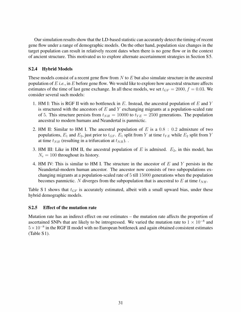
Our simulation results show that the LD-based statistic can accurately detect the timing of recentgene flow under a range of demographic models. On the other hand, population size changes in thetarget population can result in relatively recent dates when there is no gene flow or in the contextof ancient structure. This motivated us to explore alternate ascertainment strategies in Section S5.

S2.4 Hybrid Models

These models consist of a recent gene flow from N to E but also simulate structure in the ancestralpopulation ofE i.e., inE before gene flow. We would like to explore how ancestral structure affectsestimates of the time of last gene exchange. In all these models, we set tGF = 2000, f = 0.03. Weconsider several such models:

1. HM I: This is RGF II with no bottleneck in E. Instead, the ancestral population of E and Yis structured with the ancestors of E and Y exchanging migrants at a population-scaled rateof 5. This structure persists from tNH = 10000 to tY E = 2500 generations. The populationancestral to modern humans and Neandertal is panmictic.

2. HM II: Similar to HM I. The ancestral population of E is a 0.8 : 0.2 admixture of twopopulations, E1 and E2, just prior to tGF . E1 split from Y at time tY E while E2 split from Yat time tNH (resulting in a trifurcation at tNH). .

3. HM III: Like in HM II, the ancestral population of E is admixed. E2, in this model, hasNe = 100 throughout its history.

4. HM IV: This is similar to HM I. The structure in the ancestor of E and Y persists in theNeandertal-modern human ancestor. The ancestor now consists of two subpopulations ex-changing migrants at a population-scaled rate of 5 till 15000 generations when the populationbecomes panmictic. N diverges from the subpopulation that is ancestral to E at time tNH .

Table S 1 shows that tGF is accurately estimated, albeit with a small upward bias, under thesehybrid demographic models.

S2.5 Effect of the mutation rate

Mutation rate has an indirect effect on our estimates – the mutation rate affects the proportion ofascertained SNPs that are likely to be introgressed. We varied the mutation rate to 1 × 10−8 and5×10−8 in the RGF II model with no European bottleneck and again obtained consistent estimates(Table S1).

31

●

●

●

●

●

●

●

●

●●

0 1000 2000 3000 4000

010

0020

0030

0040

00

True time of gene flow (in generations)

Est

imat

ed ti

me

of g

ene

flow

Figure S2: Estimates of tGF as a function of true tGF for RGF I: We plot the mean and 2× standarderror of the estimates of tGF from 100 independent simulated datasets using ascertainment 0. Theestimates track the true tGF though the variance increases for more ancient gene flow events.

Demography Fst(Y,E) D(Y,E,N)RGF II 0.15 0.041 1987±48RGF III 0.14 0.043 1776±87RGF IV 0.15 0.04 2023 ± 56RGF V 0.07 0.04 2157±22RGF VI 0.15 0.04 2102 ± 36AS I 0.15 0.045 10128±127AS II 0.19 0.046 5070±397NGF I 0.15 -21×10−5 8847± 126NGF II 0.15 9×10−5 5800± 164HM I 0.18 0.03 2174±40HM II 0.12 0.04 2226±39HM III 0.13 0.04 2137±34HM IV 0.18 0.06 2153±36Mutation rate Fst(Y,E) D(Y,E,N)1−8 0.11 0.04 2141±415× 10−8 0.11 0.04 2134±41

Table S1: Estimates of the time of gene flow for different demographies and mutation rates.

32

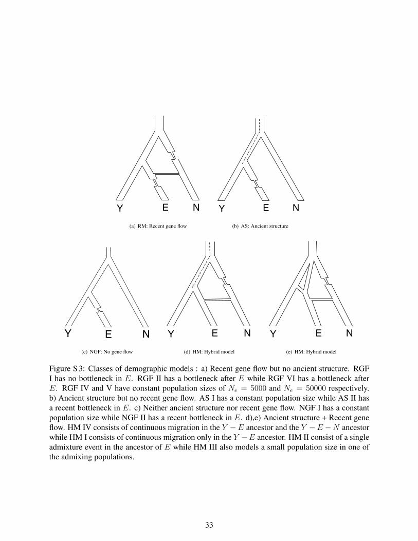
Y E N(a) RM: Recent gene flow

Y E N(b) AS: Ancient structure

Y E N(c) NGF: No gene flow

Y E N(d) HM: Hybrid model

Y E N(e) HM: Hybrid model

Figure S 3: Classes of demographic models : a) Recent gene flow but no ancient structure. RGFI has no bottleneck in E. RGF II has a bottleneck after E while RGF VI has a bottleneck afterE. RGF IV and V have constant population sizes of Ne = 5000 and Ne = 50000 respectively.b) Ancient structure but no recent gene flow. AS I has a constant population size while AS II hasa recent bottleneck in E. c) Neither ancient structure nor recent gene flow. NGF I has a constantpopulation size while NGF II has a recent bottleneck in E. d),e) Ancient structure + Recent geneflow. HM IV consists of continuous migration in the Y −E ancestor and the Y −E −N ancestorwhile HM I consists of continuous migration only in the Y −E ancestor. HM II consist of a singleadmixture event in the ancestor of E while HM III also models a small population size in one ofthe admixing populations.

33

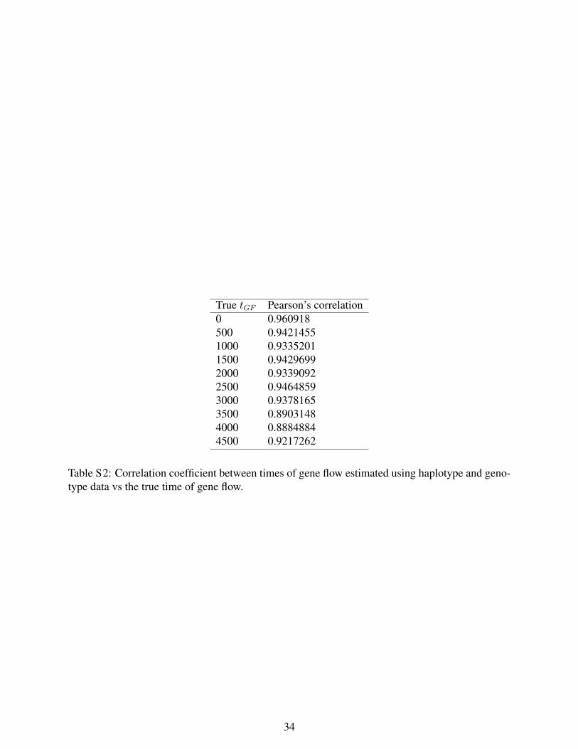
True tGF Pearson’s correlation0 0.960918500 0.94214551000 0.93352011500 0.94296992000 0.93390922500 0.94648593000 0.93781653500 0.89031484000 0.88848844500 0.9217262

Table S2: Correlation coefficient between times of gene flow estimated using haplotype and geno-type data vs the true time of gene flow.

34

S3 Correcting for uncertainties in the genetic map

In this section, we show how uncertainties in the genetic lead to a bias in the estimates of the time ofgene flow. We then show how we could correct our estimates assuming a model of map uncertainty.Our model characterizes the precision of a map by a single scalar parameter α. We estimate α fora given genetic map by comparing the distances between a pair of markers as estimated by themap to the number of crossovers that span those markers as observed in a pedigree. We propose ahierarchical model that relates α and the expected as well as observed number of crossovers andwe infer an approximate posterior distribution of α by Gibbs sampling. Finally, we show usingsimulations that this procedure is effective in providing unbiased date estimates in the presenceof map uncertainties and we apply this procedure to estimate the uncertainties of the Decode mapand Oxford LD-based map by comparing these maps to crossover events observed in a Hutteritepedigree.

S3.1 Correction

We have a genetic map G defined on m markers. Each of the m− 1 intervals is assigned a geneticdistance gi, i ∈ {1, . . . ,m − 1}. These genetic distances provide a prior on the true underlying(unobserved) genetic distances Zi. A reasonable prior on each Zi is then given by

Zi ∼ Γ (αgi, α) (1)

where α is a parameter that is specific to the map. This implies that the true genetic distance Zihas mean gi and variance gi

α. So large values of α correspond to a more precise map. The above

prior over Zi has the important property that Z1 + Z2 ∼ Γ (α(g1 + g2), α) so that α is a propertyof the map and not of the specific markers used.

Given this prior on the true genetic distances, fitting an exponential curve to pairs of markers ata given observed genetic distance g, involves integrating over the exponential function evaluatedat the true genetic distances given g i.e.,

E [exp (−tGFZ) |g] = exp (−λg) (2)

where λ is the rate of decay of D(g) as a function of the observed genetic distance g and can beestimated from the data in a straightforward manner and tGF denotes the true time of the gene flow.It also easy to see that λ will be a downward biased estimate of tGF (applying Jensen’s inequality).

We can use Equation 1 to solve for tGF (see Appendix B for details) as

tGF = α

(exp

(λ

α

)− 1

)(3)

Thus, we need to estimate α for our genetic map to obtain an estimate of tGF . As a check, notethat for a highly precise map, α� λ, we have tGF ≈ λ.

S3.2 Estimating α

Given a genetic map G defined on m markers, each of the m − 1 intervals is assigned a geneticdistance gi, i ∈ [m − 1] = {1, . . . ,m − 1}. Each interval i may contain ni − 1,≥ 0 additionalmarkers not present in G that partition interval i into a finer grid of ni intervals – each finer interval

35

is indexed by the set T = {(i, j), i ∈ [m−1], j ∈ [ni]} (e.g., these additional markers could includemarkers that are found in the observed crossovers but not in the genetic map ). Each interval (i, j)has a physical distance pi,j .

We propose the following model for taking into account the effect of map uncertainty.

Zi|α, gi ∼ Γ(αgi, α) (4)(Zi,1, . . . , Zi,ni

)|Ui, Zi ∼ (Ui,1 . . . , Ui,ni)Zi (5)

Ui = (Ui,1 . . . , Ui,ni)|β ∼ Dir(βpi,1, . . . , βpi,ni

) (6)

The “true” genetic distance Zi is related to the observed genetic distance gi through the param-eter α that is an estimate of map precision. The genetic distances of the finer intervals are obtainedby partitioning the coarse intervals – the variability of this partition is controlled by the parameterβ – β relates the physical distance to the genetic distance. When β →∞, the genetic distances ofthe finer grid are obtained by simply interpolating the coarse grid based on the physical distance.

Given the true genetic distances, we can now describe the probability of observing crossovers.Our observed data consists ofRmeioses that produce crossovers localized toLwindows {I1, . . . , IL}.Each window l ∈ [L] consists of a set of contiguous intervals Il and is known to contain a crossoverevent. Let Wi,j denote the set of windows that overlap interval (i, j).

A note on our notation: Ci,j;l is the number of crossovers in interval (i, j) that fall on windowl. We can index the C variables by sets and then we are referring to the total number of crossoversin the index set e.g., CIl;l refers to all crossovers that fall on window l within the set of intervalsIl. Omitting an index from a random variable implies summing over that index. Thus, Ci,j =∑L

l=1Ci,j;l denotes the number of crossover events in interval (i, j), Ci =∑ni

j=1Ci,j denotes thenumber of crossovers in the union of (i, j), j ∈ [ni]. −→. indicates a vector of random variables e.g.,−→C S denotes the vector of counts indexed by the elements of set S.

If we assume that the probability of multiple crossovers in any of these intervals is small, wecan use a simple probability model.

Ci,j|Zi,j ∼ Pois(RZi,j) (7)

−→C i,j;l|Ci,j ∝ δ

∑{l∈Wi,j}

Ci,j;l ≤ Ci,j, Ci,j;l ∈ {0, 1},∑{l 6∈Wi,j}

Ci,j;l = 0

(8)

Yl|Ci,j;l = δ

CIl =∑

(i,j)∈Il

Ci,j;l = 1

(9)

Here Ci,j denotes the counts of crossover events within interval (i, j) over the R meioses and is aPoisson distribution with rate parameter RZi,j . In our model, Ci,j;l is either zero or one and all thecrossovers in interval (i, j) must fall on one of the Wi,j windows that overlap (i, j). Finally, one ofthe Ci,j;l within a window l must be one for a crossover to have been detected within this window(Yl = 1).

We put an exponential prior on πα ∼ exp( 1α0

) on α. We set α0 = 10 in our inference. Whilewe can estimate β jointly, we instead fix β to∞.

To summarize, the observations in our model consist of the m − 1 observed genetic distancesGi, i ∈ [m− 1] and L observed crossovers from pedigree data Yl, l ∈ [L] (which often extend overmultiple intervals in the underlying map) as well as the total number of meioses R in the pedigree.

36

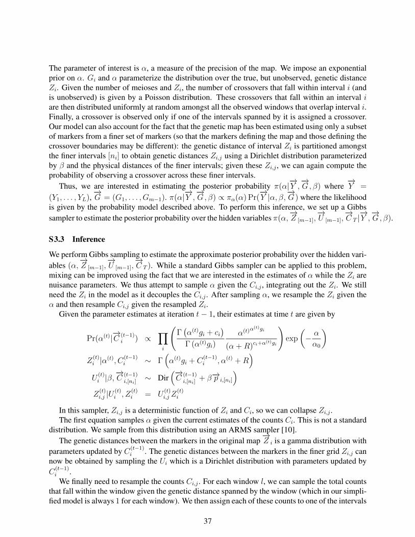
The parameter of interest is α, a measure of the precision of the map. We impose an exponentialprior on α. Gi and α parameterize the distribution over the true, but unobserved, genetic distanceZi. Given the number of meioses and Zi, the number of crossovers that fall within interval i (andis unobserved) is given by a Poisson distribution. These crossovers that fall within an interval iare then distributed uniformly at random amongst all the observed windows that overlap interval i.Finally, a crossover is observed only if one of the intervals spanned by it is assigned a crossover.Our model can also account for the fact that the genetic map has been estimated using only a subsetof markers from a finer set of markers (so that the markers defining the map and those defining thecrossover boundaries may be different): the genetic distance of interval Zi is partitioned amongstthe finer intervals [ni] to obtain genetic distances Zi,j using a Dirichlet distribution parameterizedby β and the physical distances of the finer intervals; given these Zi,j , we can again compute theprobability of observing a crossover across these finer intervals.

Thus, we are interested in estimating the posterior probability π(α|−→Y ,−→G, β) where

−→Y =

(Y1, . . . , YL),−→G = (G1, . . . , Gm−1). π(α|

−→Y ,−→G, β) ∝ πα(α) Pr(

−→Y |α, β,

−→G) where the likelihood

is given by the probability model described above. To perform this inference, we set up a Gibbssampler to estimate the posterior probability over the hidden variables π(α,

−→Z [m−1],

−→U [m−1],

−→C T |−→Y ,−→G, β).

S3.3 Inference

We perform Gibbs sampling to estimate the approximate posterior probability over the hidden vari-ables (α,

−→Z [m−1],

−→U [m−1],

−→C T ). While a standard Gibbs sampler can be applied to this problem,

mixing can be improved using the fact that we are interested in the estimates of α while the Zi arenuisance parameters. We thus attempt to sample α given the Ci,j , integrating out the Zi. We stillneed the Zi in the model as it decouples the Ci,j . After sampling α, we resample the Zi given theα and then resample Ci,j given the resampled Zi.

Given the parameter estimates at iteration t− 1, their estimates at time t are given by

Pr(α(t)|−→C

(t−1)i ) ∝

∏i

(Γ(α(t)gi + ci

)Γ (α(t)gi)

α(t)α(t)gi

(α +R)ci+α(t)gi

)exp

(− α

α0

)Z

(t)i |α(t), C

(t−1)i ∼ Γ

(α(t)gi + C

(t−1)i , α(t) +R

)U

(t)i |β,

−→C

(t−1)i,[ni]

∼ Dir(−→C

(t−1)i,[ni]

+ β−→p i,[ni]

)Z

(t)i,j |U

(t)i , Z

(t)i = U

(t)i,j Z

(t)i

In this sampler, Zi,j is a deterministic function of Zi and Ci, so we can collapse Zi,j .The first equation samples α given the current estimates of the counts Ci. This is not a standard

distribution. We sample from this distribution using an ARMS sampler [10].The genetic distances between the markers in the original map

−→Z i is a gamma distribution with

parameters updated by C(t−1)i . The genetic distances between the markers in the finer grid Zi,j can

now be obtained by sampling the Ui which is a Dirichlet distribution with parameters updated byC

(t−1)i .

We finally need to resample the counts Ci,j . For each window l, we can sample the total countsthat fall within the window given the genetic distance spanned by the window (which in our simpli-fied model is always 1 for each window). We then assign each of these counts to one of the intervals

37

within this window according to a multinomial distribution with probabilities proportional to theirgenetic distances. Finally Ci,j is obtained by summing over the counts across all windows Wi,j

that overlap interval (i, j).

Pr(C(t)Il;l|Yl = 1, Z

(t)Il

) = δ(CIl;l = 1)

C(t)i,j;l|C

(t)Il;l, Z

(t)Il∼ Mult

(1, Z

(t)Il

)C

(t)i,j |C

(t)i,j;l =

∑l∈Wi,j

C(t)i,j;l

C(t)i |C

(t)i,j =

ni∑j=1

C(t)i,j

S3.4 Simulations

To investigate the adequacy of our model of map errors, we performed coalescent simulationsusing a hotspot model of recombination. We estimated the time of gene flow using an erroneousmap. We then estimated the uncertainty of the parameter α by comparing the erroneous map to thetrue genetic map. We used the estimated α to obtain a corrected date. This procedure allows us toevaluate if our model can capture the uncertainties in the genetic map.

We simulated 100 independent 1 Mb regions using MSHOT [11]. We chose parameters forthe recombination model similar to the parameters described in [12]. We considered a modelwith tNH = 10000, tY E = 5000, tGF = 2000, constant effective population sizes of 10000 anda bottleneck in the Neandertal lineage of duration 200 generations and effective population size100. Given the true genetic map for each locus, the observed map is a noisy version generatedas follows: given the genetic map length l of each locus, the observed map has a genetic lengthG distributed according to a Gamma distribution Γ(al, a) where a parameterizes the variance ofthe map 1. Given G, the distances of the markers are obtained by interpolating from the physicalpositions.

We obtained an uncorrected estimate of the date λ using the observed genetic map. We thencompared the true genetic map and the observed map to estimate α (restricting to markers atdistances of at least 0.02 cM ) and then obtained the corrected date tGF according to Equation 3.Table S3 reports the results averaged over 10 random datasets. We see that the corrected date tGFis quite accurate when the map is accurate at a scale of 1 Mb (a ≥ 1000) and becomes less accuratewhen a ≤ 100. The results are similar when we repeated the simulations with a demography inwhich there is a 20 generation bottleneck of Ne = 100 after the gene flow.

S3.5 Results

The previous results provide us confidence that the statistical correction for map uncertainty givesaccurate estimates of the date provided the genetic map is reasonably accurate at a scale of 1 Mb.In our analyses, we therefore chose to use the Decode map [13] as well as the Oxford LD-basedmaps [14] which are known to be accurate at this scale. Another map that we considered using was

1Note that a is not the same as the parameter α that characterizes the variance of the true map given the observed map. a parameterizes thevariance in an observed map given the true map while α parameterizes the variance in the true map given an observed map

38

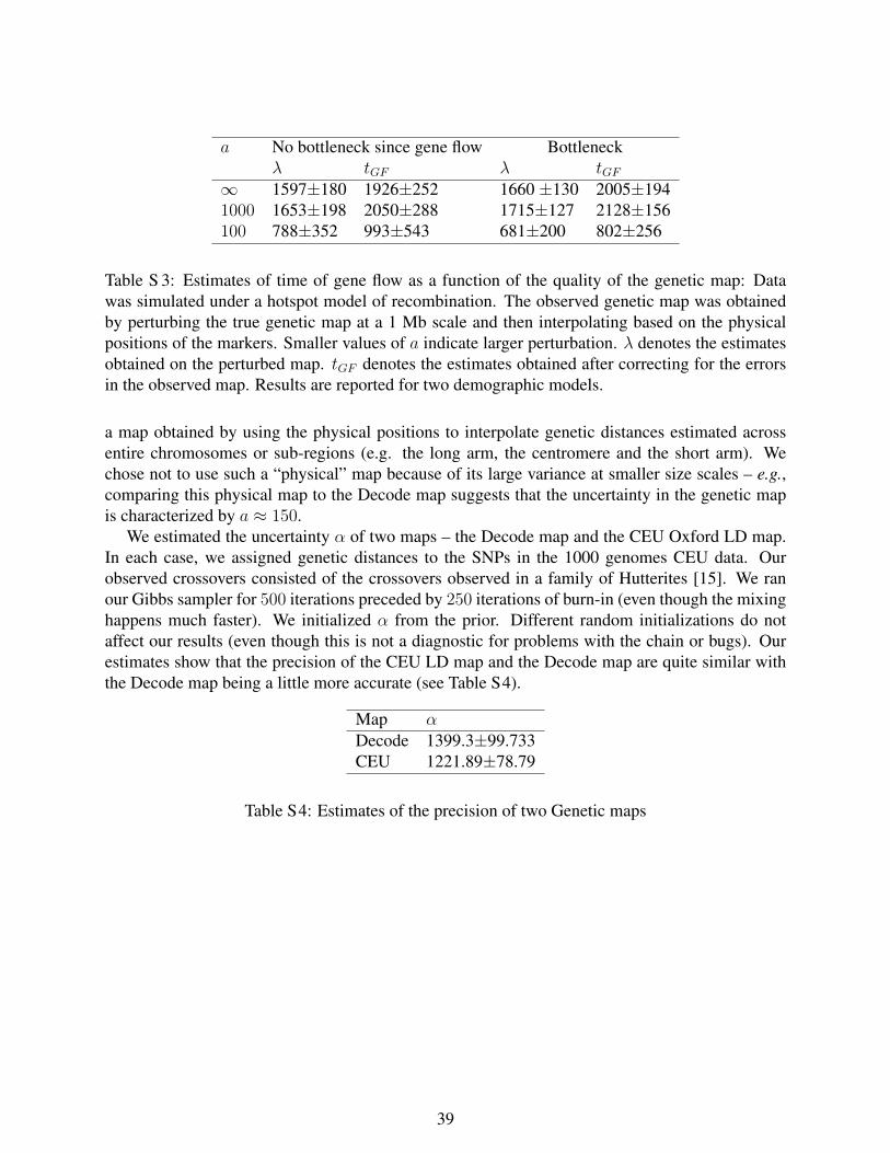
a No bottleneck since gene flow Bottleneckλ tGF λ tGF

∞ 1597±180 1926±252 1660 ±130 2005±1941000 1653±198 2050±288 1715±127 2128±156100 788±352 993±543 681±200 802±256

Table S 3: Estimates of time of gene flow as a function of the quality of the genetic map: Datawas simulated under a hotspot model of recombination. The observed genetic map was obtainedby perturbing the true genetic map at a 1 Mb scale and then interpolating based on the physicalpositions of the markers. Smaller values of a indicate larger perturbation. λ denotes the estimatesobtained on the perturbed map. tGF denotes the estimates obtained after correcting for the errorsin the observed map. Results are reported for two demographic models.

a map obtained by using the physical positions to interpolate genetic distances estimated acrossentire chromosomes or sub-regions (e.g. the long arm, the centromere and the short arm). Wechose not to use such a “physical” map because of its large variance at smaller size scales – e.g.,comparing this physical map to the Decode map suggests that the uncertainty in the genetic mapis characterized by a ≈ 150.

We estimated the uncertainty α of two maps – the Decode map and the CEU Oxford LD map.In each case, we assigned genetic distances to the SNPs in the 1000 genomes CEU data. Ourobserved crossovers consisted of the crossovers observed in a family of Hutterites [15]. We ranour Gibbs sampler for 500 iterations preceded by 250 iterations of burn-in (even though the mixinghappens much faster). We initialized α from the prior. Different random initializations do notaffect our results (even though this is not a diagnostic for problems with the chain or bugs). Ourestimates show that the precision of the CEU LD map and the Decode map are quite similar withthe Decode map being a little more accurate (see Table S4).

Map αDecode 1399.3±99.733CEU 1221.89±78.79

Table S4: Estimates of the precision of two Genetic maps

39

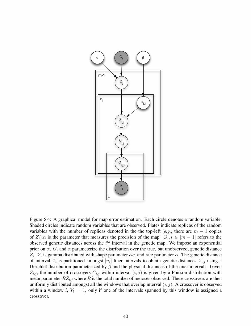
Zi

Gi

Yl

Ui,j

α

Zi,j

Ci,j

β

Ci,j;l

m-1

ni

L

Figure S 4: A graphical model for map error estimation. Each circle denotes a random variable.Shaded circles indicate random variables that are observed. Plates indicate replicas of the randomvariables with the number of replicas denoted in the the top-left (e.g., there are m − 1 copiesof Zi).α is the parameter that measures the precision of the map. Gi, i ∈ [m − 1] refers to theobserved genetic distances across the ith interval in the genetic map. We impose an exponentialprior on α. Gi and α parameterize the distribution over the true, but unobserved, genetic distanceZi. Zi is gamma distributed with shape parameter αgi and rate parameter α. The genetic distanceof interval Zi is partitioned amongst [ni] finer intervals to obtain genetic distances Zi,j using aDirichlet distribution parameterized by β and the physical distances of the finer intervals. GivenZi,j , the number of crossovers Ci,j within interval (i, j) is given by a Poisson distribution withmean parameter RZi,j where R is the total number of meioses observed. These crossovers are thenuniformly distributed amongst all the windows that overlap interval (i, j). A crossover is observedwithin a window l, Yl = 1, only if one of the intervals spanned by this window is assigned acrossover.

40

S4 Uncertainty in the date estimates

We obtain estimates of the time of gene flow taking into account all sources of uncertainty. Denotethe uncorrected date, the corrected date in generations and the corrected date in years by λ, tGFand yGF respectively.

Our model can be described as follows:

tGF = yGFG

λ = α

(log

(tGFα

)+ 1

)D(x) = a exp (−λx) + ε

ε ∼ N(0, σ2)

π(σ2) ∝ 1

σ2

where G ∼ Unif(25, 33) denotes the number of years per generation, α is the uncertainty in thegenetic map with prior given by the posterior estimated in Section S3 and a ∼ Unif(0, 1). Giventhis model, we can obtain the posterior probability distribution π(λ|D), π(tGF |D), π(yGF |D) as-suming a flat prior on each of the random variables λ, tGF , yGF respectively.

We obtain these posterior distributions by Gibbs sampling. We ran the Gibbs sampler for 200burn-in iterations followed by 1000 iterations where we sampled every 10 iterations. We computedthe posterior means and 95% credible intervals on λ, tGF and yGF .

41

S5 Effect of ascertainment

To test the robustness of our statistic, we performed coalescent-based simulations under the demo-graphic models described in Section S2. We explored two SNP ascertainments in addition to theascertainment that we described in Section S1 (which we refer to here as Ascertainment 0):

1. Ascertainment 1: SNPs for which Neandertal carries a derived allele, E is polymorphic andY does not carry a derived allele.

2. Ascertainment 2: SNPs for which Neandertal carries a derived allele, E is polymorphic andY does not carry a derived allele and SNPs for which Neandertal carries a derived allele, Edoes not carry a derived allele and Y is polymorphic.

S5.1 Recent gene flow

Under the simple demography I, Figures S 5 and S 6 show that, similar to ascertainment 0, theestimated tGF tracks the true tGF across the range of values of tGF for ascertainments 1 and 2.

We assessed the effect of demographic changes since the gene flow on the estimates of the timeof gene flow (demography RGF II of Section S2). We see in Table S5 that the bottleneck causesa downward bias in the estimated time using ascertainment 1 while ascertainment 2 is unbiased.For demography RGF III, Table S5 shows that ascertainment 1 again has a downward bias on theestimated date while ascertainment 2 has a smaller upward bias.

S5.2 Ancient structure

In the AS I model, ascertainments 1 and 2 both produce estimate close to the time of last geneexchange (9000 generations) as does ascertainment 0. In AS II, however, both ascertainments areless affected by the recent bottleneck in population E and estimate older times that are closer tothe true time of last gene exchange.

S5.3 No gene flow

Both ascertainments 1 and 2 produce dates that are quite old for both models NGF I and NGF II –the dates for NGF II are older than the estimates obtained using ascertainment 0. Ascertainment 2produces estimates that are quite close to the time of last gene flow (tNH).

Our simulation results show that in the case of recent gene flow, ascertainment 1 experiences asignificant downward bias whereas ascertainment 2 is quite accurate. In the absence of gene flowor in the case of ancient structure, both ascertainments produce estimates that are quite old andthey are more robust to population size changes in the target population relative to ascertainment0.

S5.4 Hybrid Models

For all the hybrid models, we see that all the ascertainments are quite accurate with ascertainment1 being most accurate while ascertainments 0 and 2 have a small upward bias.

42

S5.5 Effect of the mutation rate

Mutation rate has an indirect effect on our estimates – the mutation rate affects the proportion ofascertained SNPs that are likely to be introgressed. We varied the mutation rate to 1 × 10−8 and5×10−8 in the RGF II model with no European bottleneck and again obtained consistent estimates(Table S5).

S5.6 Application to 1000 genomes data

Due to the process of SNP calling that calls SNPs separately in each population, SNPs called inone of the populations may not have calls in another. This is particularly problematic for SNPs thatare polymorphic in one population and monomorphic in the other – precisely the SNPs that wewould like to ascertain in the ascertainment schemes that we described above. To overcome thislimitation, we used the following procedure to select our SNPs. For each of the SNPs that are poly-morphic in the target population, we estimated the allele frequencies in the ancestral populationdirectly from the reads that mapped to the SNP. We chose all SNPs whose derived allele frequencyin the ancestral population is estimated to be less than 1% (since we have 118 YRI chromosomes,we can resolve frequencies of the order 1

118≈ 0.01).

The ancestral allele, which was inferred using the Ensembl EPO alignment, was acquired fromthe 1000 Genomes Project FTP site. To derive the allele frequencies, we downloaded the pilot-phase alignments from the same FTP. We first adjusted each read alignment to avoid potentialartifacts caused by short sequence insertions and deletions (INDELs), and then estimated the allelefrequency by maximizing the likelihood using an estimation-maximization (EM) algorithm. Moreexactly, given we know the frequency φ(t) at the t-th iteration, the estimate for the next round is:

φ(t+1) =1

2n

n∑i=1

∑2g=0 gLi(g)f(g; 2, φ(t))∑2g=0 Li(g)f(g; 2, φ(t))

where n is the total number of samples, f(g; 2, ψ) =(2g

)ψg(1−ψ)2−g is the frequency of genotype

g under the Hardy-Weinberg equilibrium, and Li(g) is the likelihood of g for the i-th sample. Thegenotype likelihood Li(g) was computed using the MAQ error model [16].

The estimates of these different ascertainments are shown in Table S 5. We observe that, asin the simulations, the estimates obtained using ascertainment 1 are lower than the dates obtainedusing ascertainment 0 while those using ascertainment 2 are closer.

Finally, we also considered the effect of the frequency threshold of 0.10 used in Ascertainment0. Using thresholds of 0.05 and 0.20, we obtain estimates of λ = 1201(1172, 1233), 1188(1164, 1211)respectively using the Decode map. Thus, our estimates are not sensitive to the specific thresholdchosen.

43

●

●

●

●

●

●

●

●

●

●

0 1000 2000 3000 4000

010

0020

0030

0040

0050

0060

00

True time of gene flow (in generations)

Est

imat

ed ti

me

of g

ene

flow

Figure S5: Estimates of tGF as a function of true tGF for Demography RGF I: We plot the meanand 2× standard error of the estimates of tGF from 100 independent simulated datasets usingascertainment 1. The estimates track the true tGF though the variance increases for more ancientgene flow events.

44

●

●

●

●

●

●

●

●

●

●

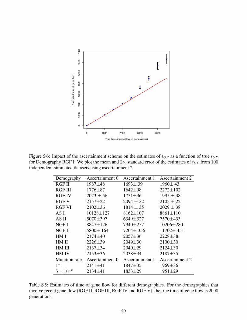
0 1000 2000 3000 4000

010

0020

0030

0040

0050

0060

0070

00

True time of gene flow (in generations)

Est

imat

ed ti

me

of g

ene

flow

Figure S6: Impact of the ascertainment scheme on the estimates of tGF as a function of true tGFfor Demography RGF I: We plot the mean and 2× standard error of the estimates of tGF from 100independent simulated datasets using ascertainment 2.

Demography Ascertainment 0 Ascertainment 1 Ascertainment 2RGF II 1987±48 1693± 39 1960± 43RGF III 1776±87 1642±98 2272±102RGF IV 2023 ± 56 1751±36 1995 ± 38RGF V 2157±22 2094 ± 22 2105 ± 22RGF VI 2102±36 1814 ± 35 2029 ± 38AS I 10128±127 8162±107 8861±110AS II 5070±397 6349±327 7570±433NGF I 8847±126 7940±257 10206±280NGF II 5800± 164 7204± 356 11702± 451HM I 2174±40 2057±36 2228±38HM II 2226±39 2049±30 2100±30HM III 2137±34 2040±29 2124±30HM IV 2153±36 2038±34 2187±35Mutation rate Ascertainment 0 Ascertainment 1 Ascertainment 21−8 2141±41 1847±35 1969±365× 10−8 2134±41 1833±29 1951±29

Table S 5: Estimates of time of gene flow for different demographies. For the demographies thatinvolve recent gene flow (RGF II, RGF III, RGF IV and RGF V), the true time of gene flow is 2000generations.

45

●

●

●

●

●

●

●

●

●

●

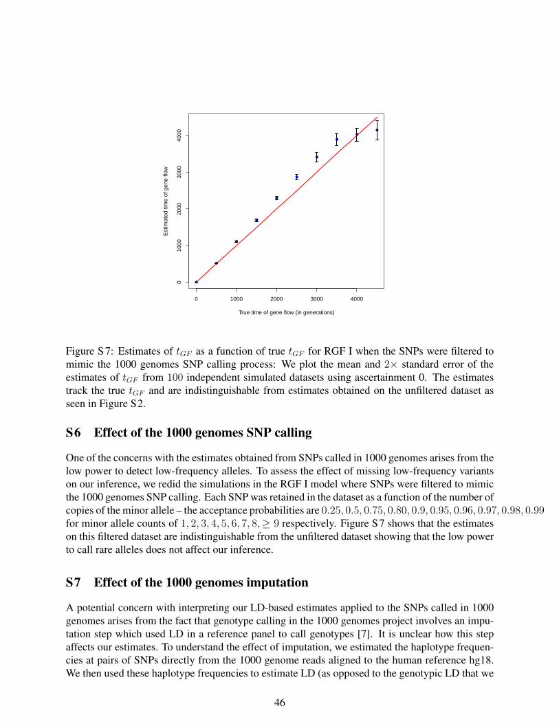
0 1000 2000 3000 4000

010

0020

0030

0040

00

True time of gene flow (in generations)

Est

imat

ed ti

me

of g

ene

flow

Figure S 7: Estimates of tGF as a function of true tGF for RGF I when the SNPs were filtered tomimic the 1000 genomes SNP calling process: We plot the mean and 2× standard error of theestimates of tGF from 100 independent simulated datasets using ascertainment 0. The estimatestrack the true tGF and are indistinguishable from estimates obtained on the unfiltered dataset asseen in Figure S2.

S6 Effect of the 1000 genomes SNP calling

One of the concerns with the estimates obtained from SNPs called in 1000 genomes arises from thelow power to detect low-frequency alleles. To assess the effect of missing low-frequency variantson our inference, we redid the simulations in the RGF I model where SNPs were filtered to mimicthe 1000 genomes SNP calling. Each SNP was retained in the dataset as a function of the number ofcopies of the minor allele – the acceptance probabilities are 0.25, 0.5, 0.75, 0.80, 0.9, 0.95, 0.96, 0.97, 0.98, 0.99for minor allele counts of 1, 2, 3, 4, 5, 6, 7, 8,≥ 9 respectively. Figure S7 shows that the estimateson this filtered dataset are indistinguishable from the unfiltered dataset showing that the low powerto call rare alleles does not affect our inference.

S7 Effect of the 1000 genomes imputation

A potential concern with interpreting our LD-based estimates applied to the SNPs called in 1000genomes arises from the fact that genotype calling in the 1000 genomes project involves an impu-tation step which used LD in a reference panel to call genotypes [7]. It is unclear how this stepaffects our estimates. To understand the effect of imputation, we estimated the haplotype frequen-cies at pairs of SNPs directly from the 1000 genome reads aligned to the human reference hg18.We then used these haplotype frequencies to estimate LD (as opposed to the genotypic LD that we

46

use in the rest of the paper) [4].Similar to the estimate of allele frequencies from the sequencing data, the two-locus haplotype

frequencies are also estimated using an EM algorithm. Given k loci, let ~h = (h1, . . . , hk) be ahaplotype where hj equals 1 if the allele at the j-th locus is derived, and equals 0 otherwise. Letη~h be the frequency of haplotype ~h satisfying

∑~h η~h = 1, where

∑~h

=1∑

h1=0

1∑h2=0

· · ·1∑

hk=0

Knowing the genotype likelihood at the j-th locus for the i-th individual L(j)i (g), we can compute

the haplotype frequencies iteratively with:

η(t+1)~h

=η(t)~h

n

n∑i=1

∑~h′ η

(t)~h′

∏kj=1 L

(j)i (hj + h′j)∑

~h′,~h′′ η(t)~h′η(t)~h′′

∏j L

(j)i (h′j + h′′j )

(10)

We restricted our analysis to SNPs chosen using ascertainment 0 and used the Decode map todetermine our genetic distances. We fitted an exponential with an affine term to the decay curveto obtain an uncorrected date λ = 1210, consistent with λ = (1179, 1233) obtained using thegenotypes called in 1000 genomes. Thus, the genotype imputation does not appear to be a majorsource of bias in our estimates.

47

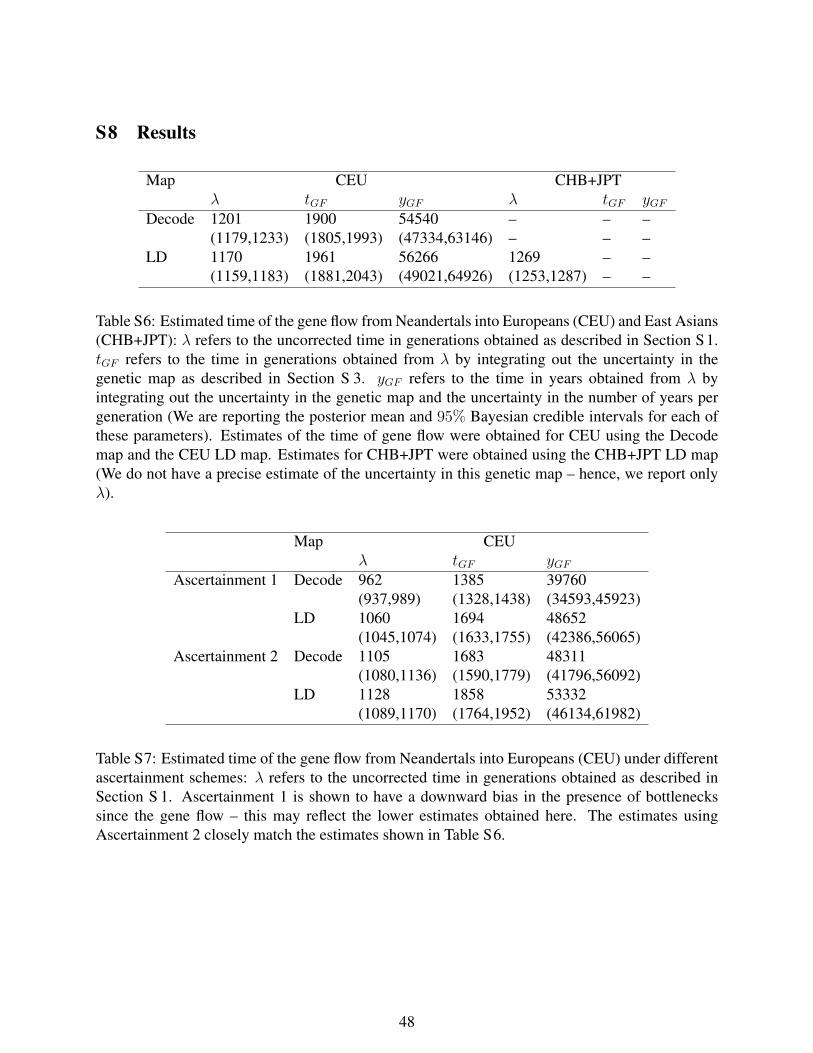
S8 Results

Map CEU CHB+JPTλ tGF yGF λ tGF yGF

Decode 1201 1900 54540 – – –(1179,1233) (1805,1993) (47334,63146) – – –

LD 1170 1961 56266 1269 – –(1159,1183) (1881,2043) (49021,64926) (1253,1287) – –

Table S6: Estimated time of the gene flow from Neandertals into Europeans (CEU) and East Asians(CHB+JPT): λ refers to the uncorrected time in generations obtained as described in Section S1.tGF refers to the time in generations obtained from λ by integrating out the uncertainty in thegenetic map as described in Section S 3. yGF refers to the time in years obtained from λ byintegrating out the uncertainty in the genetic map and the uncertainty in the number of years pergeneration (We are reporting the posterior mean and 95% Bayesian credible intervals for each ofthese parameters). Estimates of the time of gene flow were obtained for CEU using the Decodemap and the CEU LD map. Estimates for CHB+JPT were obtained using the CHB+JPT LD map(We do not have a precise estimate of the uncertainty in this genetic map – hence, we report onlyλ).

Map CEUλ tGF yGF

Ascertainment 1 Decode 962 1385 39760(937,989) (1328,1438) (34593,45923)

LD 1060 1694 48652(1045,1074) (1633,1755) (42386,56065)

Ascertainment 2 Decode 1105 1683 48311(1080,1136) (1590,1779) (41796,56092)

LD 1128 1858 53332(1089,1170) (1764,1952) (46134,61982)

Table S7: Estimated time of the gene flow from Neandertals into Europeans (CEU) under differentascertainment schemes: λ refers to the uncorrected time in generations obtained as described inSection S 1. Ascertainment 1 is shown to have a downward bias in the presence of bottleneckssince the gene flow – this may reflect the lower estimates obtained here. The estimates usingAscertainment 2 closely match the estimates shown in Table S6.

48

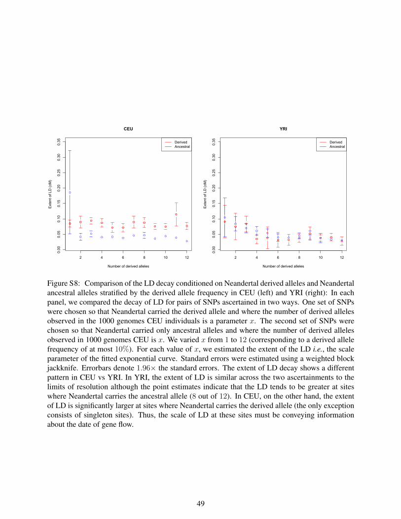
2 4 6 8 10 12

0.00

0.05

0.10

0.15

0.20

0.25

0.30

0.35

Number of derived alleles

Ext

ent o

f LD

(cM

)

DerivedAncestral

CEU

2 4 6 8 10 12

0.00

0.05

0.10

0.15

0.20

0.25

0.30

0.35

Number of derived alleles

Ext

ent o

f LD

(cM

)

DerivedAncestral

YRI

Figure S8: Comparison of the LD decay conditioned on Neandertal derived alleles and Neandertalancestral alleles stratified by the derived allele frequency in CEU (left) and YRI (right): In eachpanel, we compared the decay of LD for pairs of SNPs ascertained in two ways. One set of SNPswere chosen so that Neandertal carried the derived allele and where the number of derived allelesobserved in the 1000 genomes CEU individuals is a parameter x. The second set of SNPs werechosen so that Neandertal carried only ancestral alleles and where the number of derived allelesobserved in 1000 genomes CEU is x. We varied x from 1 to 12 (corresponding to a derived allelefrequency of at most 10%). For each value of x, we estimated the extent of the LD i.e., the scaleparameter of the fitted exponential curve. Standard errors were estimated using a weighted blockjackknife. Errorbars denote 1.96× the standard errors. The extent of LD decay shows a differentpattern in CEU vs YRI. In YRI, the extent of LD is similar across the two ascertainments to thelimits of resolution although the point estimates indicate that the LD tends to be greater at siteswhere Neandertal carries the ancestral allele (8 out of 12). In CEU, on the other hand, the extentof LD is significantly larger at sites where Neandertal carries the derived allele (the only exceptionconsists of singleton sites). Thus, the scale of LD at these sites must be conveying informationabout the date of gene flow.

49

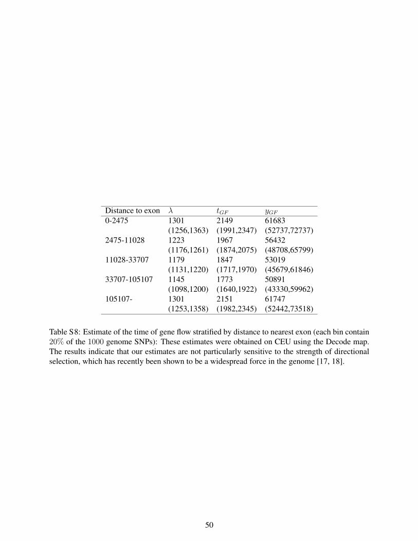
Distance to exon λ tGF yGF0-2475 1301 2149 61683

(1256,1363) (1991,2347) (52737,72737)2475-11028 1223 1967 56432

(1176,1261) (1874,2075) (48708,65799)11028-33707 1179 1847 53019

(1131,1220) (1717,1970) (45679,61846)33707-105107 1145 1773 50891

(1098,1200) (1640,1922) (43330,59962)105107- 1301 2151 61747

(1253,1358) (1982,2345) (52442,73518)

Table S8: Estimate of the time of gene flow stratified by distance to nearest exon (each bin contain20% of the 1000 genome SNPs): These estimates were obtained on CEU using the Decode map.The results indicate that our estimates are not particularly sensitive to the strength of directionalselection, which has recently been shown to be a widespread force in the genome [17, 18].

50

A Exponential decay of the statistic

We are interested in how the linkage disequilibrium varies as a function of genetic distance x. Weconsider two SNPs that are polymorphic at time 0 in the past. The evolution of the alleles at thetwo SNPs can be described by the two-locus Wright-Fisher diffusion in a space parameterized byXt = (p, q,D)t i.e., the allele frequencies at each SNP at time t and measure of LD D at the twoSNPs [19]. At time t, the average LD is denoted EDt(x) (we assume that the population is not atequilibrium so that ED 6= 0).

We are interested in the average linkage-disequilibrium at a time t given the state of the systemat time 0 : u(t, x) = E [Dt|X0 = x].

We also denote the effective population size at time t by N(t) = ν(t)N0 and the probability ofrecombination between the two loci by r.

The evolution of u(t, x) is given by∂u

∂t= Lu (11)

where L is the generator for this diffusion with initial condition

u(0, x) = D0

and boundary conditions

u(t, (0, q, d)) = u(t, (p, 0, d) = 0

∂u

∂d(p, q, dmax(p, q)) =

∂y

∂d(p, q, dmin(p, q)) = 0

∂u

∂t= Lu = −

[r +

1

2ν(t)N0

]u (12)

The solution to Equation 12 is given by

u(t, x) = D0 exp

(− 1

2N0

∫ t

0

dτ

ν(τ)

)exp (−rt)

So we have

EDt = ED0 exp

(− 1

2N0

∫ t

0

dτ

ν(τ)

)exp (−rt) (13)

If we choose SNPs that that arose in the N lineage and introgressed into E tGF generations ago(i.e., these are SNPs that were monomoprhic in E before the gene flow), Equation 13 says thatthe average D observed between all such pairs of SNPs at a given genetic distance r depends onthree factors – the average LD at time 0 (ED0), the factor exp

(− 1

2N0

∫ t0

dτν(τ)

)that accounts for

changes in population sizes since gene flow and the factor exp (−rt) that accounts for the decayin LD. Terms 1 and 3 depend on r while term 2 does not. Further, since we ascertain SNPs thatarose in the N lineage and introgressed into E, ED0 will depend on the average value of D inthe introgressing Neandertals scaled by their admixing proportion. While ED0 still depends onthe genetic distance r, for highly-bottlenecked populations such as the Neandertals ,in which theprobability of coalescence has been estimated to be at least 0.65 [8], this term could be assumed

51

to be a constant in r. We can then approximate the relation between the average D and the geneticdistance r by the exponential term exp (−rtGF ) where the intercept of the exponential (its value atr = 0) depends on the population history. Thus, rate of decay of the expectation of D as a functionof r would correspond in this case to tGF and could provide a robust method to date gene flow.

Equation 13 implies that changes in the effective population size since the gene flow will notchange the relation between EDt and r. Since we have chosen SNPs that are monomorphic in Ebefore the time of gene flow, demographic history in E before gene flow also does not affect EDt.However, this result has limitations when applied to polymorphism data. First, this result requiresprecisely ascertaining SNPs that arose in N and introgressed. Imperfections in the ascertainmentcan make the procedure sentive to demography. Further, the expectation needs to be computedover all pairs of SNPs that were polymorphic at time 0 even if these SNPs may have fixed or goneextinct since. Such SNPs would be hard to ascertain using present-day genomes. Second, if thedrift since gene flow is high or the level of gene flow is low, the intercept of the exponential curvedecreases making it harder to estimate its rate of decay from data

52

B Proof of Equation 3 in Section S3

Equation 2 is given byE [exp (−tGFZ) |g] = exp (−λg) (14)

whereZ ∼ Γ (αg, α) (15)

We can explicitly compute the LHS of 2

E [exp (−tGFZ) |g] =ααg

Γ(αg)

∫dzzαg−1 exp (−αz) exp (−tGF z)

=ααg

Γ(αg)

Γ(αg)

(tGF + α)αg

= exp

(−α log

((tGFα

)+ 1

)g

)(16)

Equating the coefficients of g in the RHS of Equation 2 and 16 gives us Equation 3.

53

References

[1] Catarina Pinho and Jody Hey. Divergence with gene flow: Models and data. Annual Reviewof Ecology, Evolution, and Systematics, 41(1):215–230, 2010.

[2] C. A. Machado, R. M. Kliman, J. A. Markert, and J. Hey. Inferring the history of specia-tion from multilocus DNA sequence data: the case of Drosophila pseudoobscura and closerelatives. Mol. Biol. Evol., 19:472–488, Apr 2002.

[3] Priya Moorjani, Nick Patterson, Joel N. Hirschhorn, Alon Keinan, Li Hao, Gil Atzmon, Ed-ward Burns, Harry Ostrer, Alkes L. Price, and David Reich. The history of african gene flowinto southern europeans, levantines, and jews. PLoS Genet, 7(4):e1001373, 04 2011.

[4] Lewontin Richard and Kojima Ken-Ichi. The evolutionary dynamics of complex polymor-phisms. Evolution, 14:458 – 472, 1960.

[5] Richard E. Green, Johannes Krause, Adrian W. Briggs, Tomislav Maricic, Udo Stenzel, Mar-tin Kircher, Nick Patterson, Heng Li, Weiwei Zhai, Markus Hsi-Yang Fritz, Nancy F. Hansen,Eric Y. Durand, Anna-Sapfo Malaspinas, Jeffrey D. Jensen, Tomas Marques-Bonet, CanAlkan, Kay Prufer, Matthias Meyer, Hernan A. Burbano, Jeffrey M. Good, Rigo Schultz,Ayinuer Aximu-Petri, Anne Butthof, Barbara Hober, Barbara Hoffner, Madlen Siegemund,Antje Weihmann, Chad Nusbaum, Eric S. Lander, Carsten Russ, Nathaniel Novod, JasonAffourtit, Michael Egholm, Christine Verna, Pavao Rudan, Dejana Brajkovic, Zeljko Kucan,Ivan Gusic, Vladimir B. Doronichev, Liubov V. Golovanova, Carles Lalueza-Fox, Marco de laRasilla, Javier Fortea, Antonio Rosas, Ralf W. Schmitz, Philip L. F. Johnson, Evan E. Eich-ler, Daniel Falush, Ewan Birney, James C. Mullikin, Montgomery Slatkin, Rasmus Nielsen,Janet Kelso, Michael Lachmann, David Reich, and Svante Paabo. A draft sequence of theneandertal genome. Science, 328(5979):710–722, 2010.

[6] Weir Bruce. Genetic Data Analysis III. Sinauer Associates, 3rd edition, 2010.

[7] Richard M. Durbin and 1000 Genomes Project Consortium. A map of human genome varia-tion from population-scale sequencing. NATURE, 467(7319):1061–1073, OCT 28 2010.

[8] D. Reich, R. E. Green, M. Kircher, J. Krause, N. Patterson, E. Y. Durand, B. Viola, A. W.Briggs, U. Stenzel, P. L. Johnson, T. Maricic, J. M. Good, T. Marques-Bonet, C. Alkan,Q. Fu, S. Mallick, H. Li, M. Meyer, E. E. Eichler, M. Stoneking, M. Richards, S. Talamo,M. V. Shunkov, A. P. Derevianko, J. J. Hublin, J. Kelso, M. Slatkin, and S. Paabo. Genetichistory of an archaic hominin group from Denisova Cave in Siberia. Nature, 468:1053–1060,Dec 2010.

[9] Jeffrey D. Wall, Kirk E. Lohmueller, and Vincent Plagnol. Detecting ancient admixture andestimating demographic parameters in multiple human populations. Molecular Biology andEvolution, 2009.

[10] W. R. Gilks, N. G. Best, and K. K. C. Tan. Adaptive rejection metropolis sampling. AppliedStatistics, 44:455–472, 1995.

[11] Garrett Hellenthal and Matthew Stephens. mshot: modifying hudson’s ms simulator to incor-porate crossover and gene conversion hotspots. Bioinformatics, 23(4):520–521, 2007.

54

[12] Garrett Hellenthal, Adam Auton, and Daniel Falush. Inferring human colonization historyusing a copying model. PLoS Genet, 4(5):e1000078, 05 2008.

[13] A. Kong, G. Thorleifsson, D. F. Gudbjartsson, G. Masson, A. Sigurdsson, A. Jonasdottir,G. B. Walters, A. Jonasdottir, A. Gylfason, K. T. Kristinsson, S. A. Gudjonsson, M. L. Frigge,A. Helgason, U. Thorsteinsdottir, and K. Stefansson. Fine-scale recombination rate differ-ences between sexes, populations and individuals. Nature, 467:1099–1103, Oct 2010.

[14] Simon Myers, Leonardo Bottolo, Colin Freeman, Gil McVean, and Peter Donnelly. Afine-scale map of recombination rates and hotspots across the human genome. Science,310(5746):321–324, 2005.

[15] G. Coop, X. Wen, C. Ober, J. K. Pritchard, and M. Przeworski. High-resolution mappingof crossovers reveals extensive variation in fine-scale recombination patterns among humans.Science, 319:1395–1398, Mar 2008.

[16] H. Li, J. Ruan, and R. Durbin. Mapping short DNA sequencing reads and calling variantsusing mapping quality scores. Genome Res., 18:1851–1858, Nov 2008.

[17] Graham McVicker, David Gordon, Colleen Davis, and Phil Green. Widespread genomicsignatures of natural selection in hominid evolution. PLoS Genet, 5(5):e1000471, 05 2009.

[18] James J. Cai, J. Michael Macpherson, Guy Sella, and Dmitri A. Petrov. Pervasive hitchhikingat coding and regulatory sites in humans. PLoS Genet, 5(1):e1000336, 01 2009.

[19] T. Ohta and M. Kimura. Linkage disequilibrium at steady state determined by random geneticdrift and recurrent mutation. Genetics, 63:229–238, Sep 1969.

55