THE CREATION OF SYNTHETIC POWER GRIDS: PRELIMINARY CONSIDERATIONS

BY

ADAM B. BIRCHFIELD

THESIS

Submitted in partial fulfillment of the requirements for the degree of Master of Science in Electrical and Computer Engineering

in the Graduate College of the University of Illinois at Urbana-Champaign, 2016

Urbana, Illinois

Adviser:

Professor Thomas J. Overbye

ii

Abstract

This thesis presents preliminary considerations and an initial methodology for

the systematic creation of synthetic power system test cases. The synthesized grids are

built to match statistical characteristics found in actual power grids, but they do not

correspond to any real grid and are thus free from confidentiality requirements. First,

substations are geographically placed on a selected territory, synthesized from public

information about the underlying population and generation plants. A clustering

technique is employed, which ensures the synthetic substations meet realistic

proportions of load and generation, among other constraints. Next, a network of

transmission lines is added. This thesis describes several structural statistics to be used

in characterizing real power system networks, including connectivity, Delaunay

triangulation overlap, dc power flow analysis, and line intersection rate. The thesis

presents a methodology to generate synthetic line topologies with realistic parameters

which satisfy these criteria. Then, the test cases can be augmented with additional

complexities to build large, realistic cases. An application to geomagnetic disturbance

analysis is discussed as an example. The thesis illustrates the method with two example

test cases, one with 150 buses and the other with 2000 buses. The methodology for

creating each is shown, and the characteristics of these cases are validated against the

observations from real cases.

iii

Acknowledgments

I gratefully acknowledge funding for my education and research from the

Advanced Research Projects Agency-Energy (ARPA-E), U.S. Department of Energy

(Award DE-AR0000714), from Bonneville Power Administration (Project TIP-359),

and from the University of Illinois ECE Distinguished Research Fellowship.

I thank my adviser, Prof. Thomas J. Overbye, for his vision and guidance of

this work, and my colleagues Ti Xu, Kathleen M. Gegner, and Komal S. Shetye, for

their assistance. Building these synthetic networks is a team effort.

I am grateful to my father and mother, Ken and Denise Birchfield, who love

me and encourage me, along with my sister Audrey, brother Jack, and sister Carrie,

and grandparents Jerry and Jackie Birchfield and Gary and Caroline Sayre. My family

are my best friends.

I am thankful for the friendship of Pastor Luke Herche and many others at All

Souls Presbyterian Church in Urbana, Illinois, my home for a delightful, short year.

I am thankful, most of all, to the Lord Jesus Christ, who made me, redeemed

me, and sustains me by his grace. The benefit and motivation of this work is that I

may use my talents, which are gifts from him, and till the ground in this small corner

of his world, to his glory.

iv

Table of Contents

Chapter 1: Introduction to Synthetic Power Grids ........................................................... 1

Chapter 2: Review of Previous Research ............................................................................ 6

Chapter 3: Loads, Generators, and Substations ................................................................. 9

Chapter 4: Buses, Transformers, and Transmission Lines ............................................. 16

Chapter 5: Network Topology and the Delaunay Triangulation .................................. 22

Chapter 6: Application to Geomagnetic Disturbance (GMD) Analysis ...................... 41

Chapter 7: Voltage Control, Transient Stability and Other Future Work ................... 48

Chapter 8: Discussion and Conclusion ............................................................................. 50

References ............................................................................................................................. 52

1

Chapter 1: Introduction to Synthetic Power Grids

The size of an electric power system is often measured by the number of buses,

or circuit nodes, used when the system is modeled for computer simulations. The

Eastern Interconnect in North America, for example, is represented with about 70,000

buses in a recent model. Researchers often run simulations on models ranging from

ultra-simplified two-bus equivalents up to full models of an interconnect-wide actual

grid. Small grid models with less than 100 buses are much more manageable for the

early stages of a research endeavor, but in order to be useful for application in a real

power system, innovations must be proven on grid models that are realistic, and

therefore, large.

Power systems are critical infrastructure, so information contained in a

simulation model of a real grid, such as the Eastern Interconnect, is treated as

confidential. As a result, large grid models, which are essential to developing, testing,

verifying, and demonstrating innovative grid research, can be hard to obtain. For

legitimate security reasons, there are heavy restrictions that limit which researchers are

allowed access to which grid models, and what they can do with the information

2

contained in them. For researchers who are able to access actual grid models through

non-disclosure agreements, the successful results they report in academic publications

cannot be directly verified by peers, unless the peers are approved to access the same

models through a separate non-disclosure agreement. The scientific principle of the

reproducibility of results is diminished.

For decades, public test cases have been a hallmark of power systems

simulation research. Certain grid models are standardized, in some sense, and made

widely available without any confidentiality restrictions, usually because the model is

based on an older version of a real grid, or has been modified significantly from the

real grid behind it, or never represented an actual grid in the first place. Such models

are well suited to the reproducibility of results; they stimulate innovation and are

ultimately valuable to the industry as a whole. The most notable and widely recognized

examples are the IEEE test cases, which vary in size from 14 to 300 buses. Any

academic periodical on the topic of power systems engineering will contain many

papers featuring simulation results on this handful of small grid models. There are

others too, but in general, existing public grid models are limited in their size and

complexity compared to actual grid models, and do not fully meet the needs of today’s

power systems research community.

Synthetic power grids are entirely fictitious public test cases, built

systematically to match important characteristics of the actual grid, including size and

complexity. This thesis describes preliminary considerations in an approach to build

synthetic power grids. Past test cases were built by hand, usually by simplifying and

obscuring the details of an outdated actual power grid model. In contrast, the benefit

of these totally synthetic grid models is that no simplification or obfuscation is

3

necessary; the grids are detailed and clear like the real grid, except they are not real.

Since size and quantity are principle objectives, the creation process must be

automated to some degree. Placing 70,000 buses by hand is impossible. The focus of

this thesis, therefore, is not on the development of a set of individual synthetic grids,

but on the development of the process by which many grids of various sizes could be

produced. Two example cases are described, one of 150 buses and one of 2000 buses,

but the foundational synthesis principles are the key contribution.

Synthetic grids must be not only large, but realistic and complex. The first

requirement is a challenge because little previous research has specified the defining

characteristics which make a grid realistic. This thesis begins to answer that question,

by selecting statistics of real grids’ proportions, structure, and solution that can be

matched in new test cases. Complexity in test cases refers to the presence of atypical

elements and controls with which the actual grid models are rife, including FACTS

devices, HVDC lines, phase-shifting transformers, remote bus voltage control by tap-

changing transformer windings, and transformer impedance correction tables.

Matching the real grid’s characteristics on average is not sufficient; outliers also must

be added. Additional data such as dynamic models and geomagnetic disturbance

models fall under complexity as well. Fortunately, these are separable subproblems

which can be solved by augmenting the basic case with additional data. This thesis

focuses on the base case and provides examples of additional complexities.

The approach taken starts with realistic geographic coordinates, and there are

several reasons for this, despite the fact that such data is not needed for basic power

flow solutions, nor is it typical for existing test cases. First, all real grids have a

geographic location, and that location underlies every aspect of the network’s

4

development, from the local customer demand to which buses are close enough to be

connected by a transmission line. Visualization research for power grids, a growing

field of study, needs grids with system one-line diagrams. Geographic locations are not

easily forced onto an established network. Another growing area of research, the study

of geomagnetically induced currents (GICs) on the power grid, needs geolocations for

its calculations. Finally, putting the grids on geographic areas familiar to users adds to

the subjective realism of the case, allows the harnessing of existing public data in the

area, and gives reasonable distance approximations for calculating transmission line

impedances. The synthetic grids look and feel real, even though they have no relation

to the actual grid in the location where they are placed.

There are three parts to the process contained in this thesis. First, substations

are placed with loads and generators. This step makes use of public energy and

population data on the selected geographic footprint and uses clustering methods to

match selected characteristics of real substations. The network topology is step two,

where buses, transformers, and transmission lines connect the generators to the loads

in a way that matches topological, geographic, and electrical metrics of realism. Lastly,

the base case is augmented with additional complexities, for which a few examples are

given in this thesis but much future work remains.

The evolution of real-world power grids is a process influenced by factors far

too numerous to model comprehensively. The final network circuit model is

determined by engineering decisions considering where right-of-ways are physically

available, the substation size a certain terrain will allow, what natural resources can be

used for generators, and of course, customer-specific needs. Compounding this

complexity are factors such as financial restrictions, corporate agreements, and

5

political regulations. When considering the present grid’s development, the biggest

complication is that the network was built over many decades, while customer needs

and government regulations shifted, and while each generation of engineers planned

for what they predicted the future would require. It is not the author’s purpose to fully

model the history of this highly reliable but diversely constructed infrastructure. This

thesis will show, however, that in creating fictitious test cases it is possible to capture

critical qualities of real grids such that the synthetic grids are nearly as useful for testing

research algorithms as the real grid models themselves.

6

Chapter 2: Review of Previous Research

The standard IEEE power flow test cases can be found from multiple online

archives [1], [2]. The 14-bus case, the 30-bus case, the 57-bus case, and the 118-bus

case were developed as approximations of the 1960s grid in the midwestern United

States. The 24-bus case, 39-bus case, and the 300-bus case, depicted in Fig. 1, were

also based on real grids. In general, these systems represent a type of grid which is now

many decades old, with many synchronous condensers, for example, and very few

power electronics based devices. These cases and others have become common for

use in power systems research.

A few researchers have taken the approach of developing a model

approximating the actual grid based on public information released. Recently, [3]

created an 8-zone market-oriented test system based in New England. An effort

described by [4] used public information from utilities and regulatory agencies to

develop an approximate dc power flow model of the continental European grid. This

approach differs from the concept of synthetic networks, which do not attempt to

approximate the actual grid, but only to create fictitious models with characteristics

7

which match those of actual grids. The network of [4] is large with 1500 buses and is

designed for optimal power flow and locational marginal price analysis. However, it

contains neither specifications sufficient for an ac power flow solution, nor other

complexities which would be present in a real power system.

In the last twenty years, attention has focused increasingly on analyzing the

circuit structure of electric power transmission systems as a complex graph. Viewing

electric buses as vertices connected by electric branches as edges, this paradigm enables

comparing the power grid with a variety of real-world technological, biological, and

social networks. Two salient properties of many real networks are highlighted in [5]:

high clustering and a low average path length between any two nodes. Networks with

these properties are called Small World networks, and they can be modeled as a regular

Fig. 1. One-line diagram of the IEEE 300-bus test case. This is among the largest existing public test cases.

2 40 MW

4 Mvar

2

241 MW 89 Mvar

2

73 MW 0 Mvar

3

428 MW 232 Mvar

3 173 MW 99 Mvar

2 60 MW

24 Mvar

3

22 MW 16 Mvar

1 58 MW 14 Mvar

1 96 MW 43 Mvar

1

20 MW 0 Mvar

1

120 MW 41 Mvar

1

56 MW

15 Mvar

2

2 0 MW

0 Mvar

2

482 MW 205 Mvar

2

827 MW

135 Mvar

2

274 MW

100 Mvar

2

2

764 MW 291 Mvar

2

2

300 MW 96 Mvar

2

35 MW 15 Mvar

2

2

515 MW

83 Mvar

2

276 MW 59 Mvar

2

28 MW 12 Mvar

2

2

89 MW 35 Mvar

3

448 MW 143 Mvar

2

60 MW 24 Mvar

2

2

137 MW 17 Mvar

3

7 MW 2 Mvar

3

3

3

800 MW 72 Mvar

1

45 MW

12 Mvar

1

28 MW 9 Mvar1

2

69 MW

49 Mvar

1

160 MW 60 Mvar

1

561 MW 220 Mvar

1

2

1

1

58 MW 10 Mvar

1

127 MW 23 Mvar

1

1

81 MW

23 Mvar

1

77 MW 1 Mvar

1

21 MW 7 Mvar

1 37 MW

13 Mvar

1

28 MW

7 Mvar

1 1

90 MW

49 Mvar

3

489 MW 53 Mvar

2

74 MW 29 Mvar

3

3

96 MW

7 Mvar

3

171 MW

70 Mvar

3

328 MW 188 Mvar

3

404 MW 212 Mvar

3

285 MW

100 Mvar

3

572 MW 244 Mvar

3

27 MW 12 Mvar

3

43 MW 14 Mvar

3

64 MW 21 Mvar

3

3

35 MW 12 Mvar

3

100 MW 75 Mvar

3

8 MW 3 Mvar

1

-21 MW -14 Mvar

3

3

255 MW 149 Mvar

3

3

72 MW 24 Mvar

3

3

0 MW -5 Mvar

33

176 MW

105 Mvar

3

12 MW 2 Mvar

3

47 MW 26 Mvar

3

7 MW 2 Mvar

3

38 MW 13 Mvar

1

1

39 MW

9 Mvar

1

14 MW

1 Mvar

1

218 MW 106 Mvar

1

155 MW 18 Mvar

1

5 MW 0 Mvar

1

112 MW 0 Mvar

2

2

2

3

33

159 MW

107 Mvar

410 MW 40 Mvar

2

17 MW 9 Mvar

2

55 MW 18 Mvar

2

183 MW 44 Mvar

1

148 MW 33 Mvar

1

1

78 MW 0 Mvar

1

32 MW 0 Mvar

1

9 MW 0 Mvar1

50 MW 0 Mvar

1

31 MW 0 Mvar

1

83 MW

21 Mvar

1

63 MW 0 Mvar

1

20 MW

0 Mvar

1

26 MW 0 Mvar

1

18 MW 0 Mvar

1

595 MW

120 Mvar

1

41 MW 14 Mvar 1

69 MW 13 Mvar

1

116 MW

-24 Mvar

1

2 MW -13 Mvar

1

2 MW

-4 Mvar

1

-15 MW 26 Mvar

1

25 MW -1 Mvar

1

55 MW

6 Mvar

11

1

1

85 MW 32 Mvar

1

1

46 MW -21 Mvar

1

86 MW 0 Mvar

1 1

195 MW

29 Mvar

1

1

58 MW 12 Mvar

1

1

1

1

1

1

1

1

1

56 MW 20 Mvar

1

1

1

1

70 MW

30 Mvar

1

1

227 MW

110 Mvar 1

30 MW

1 Mvar

1

1

98 MW 20 Mvar

1

50 MW

17 Mvar

1

-11 MW -1 Mvar

1

22 MW 10 Mvar

1

10 MW

1 Mvar

1

14 MW

3 Mvar

1

69 MW 3 Mvar

1 28 MW -20 Mvar

1

145 MW -35 Mvar

1

61 MW 28 Mvar

1

-5 MW

5 Mvar

1

353 MW 130 Mvar

1

92 MW 26 Mvar

1

41 MW 19 Mvar

1

1

1

1

1

1

1

1

1

116 MW 38 Mvar

1

57 MW

19 Mvar

1

224 MW 71 Mvar

1

1

208 MW 107 Mvar

1

74 MW 28 Mvar

1

1

48 MW 14 Mvar

1

1

1

11

1

44 MW 0 Mvar

1

66 MW 0 Mvar

1

1

1 3 MW 1 Mvar

1

1 MW 0 Mvar

1

1 11

1

5 MW 2 Mvar

1

2 MW 1 Mvar

1

1 1 MW 0 Mvar

1

0 MW 0 Mvar

1

0 MW 0 Mvar

1

2 MW 1 Mvar

1

1 MW 0 Mvar

1

2 MW 1 Mvar

1

2 MW

1 Mvar

1

2 MW 1 Mvar

1

3 MW 1 Mvar

1

2 MW 1 Mvar

1

3 MW 1 Mvar

1

1 MW 0 Mvar

1

2 MW 1 Mvar

1

1 MW 0 Mvar

1

1

1 30 MW 23 Mvar

111

1

1 MW 0 Mvar

1

1 MW 0 Mvar

1

17 MW 0 Mvar

1

4 MW 1 Mvar

1

16 MW 0 Mvar

1

60 MW 0 Mvar

1

1 MW 0 Mvar

1

40 MW

0 Mvar

1

67 MW 0 Mvar

1

83 MW

0 Mvar

22

2

2

14 MW

650 Mvar

2

2

2

535 MW

55 Mvar

2

229 MW

12 Mvar

2

78 MW 1 Mvar

2

58 MW 5 Mvar

2

381 MW 37 Mvar

22

2

2

2

2

2 169 MW 42 Mvar

2

388 MW

115 Mvar

145 MW 58 Mvar

2

56 MW 25 Mvar

2

2

24 MW 14 Mvar

2 2

2

63 MW

25 Mvar

2

2

2

2

2

427 MW 174 Mvar

2

5 MW 4 Mvar

2

176 MW 83 Mvar

2

2

163 MW 43 Mvar

2

595 MW 83 Mvar

26 MW 0 Mvar

2

2

2

2

85 MW

24 Mvar

2

33 MW

17 Mvar

2

2

124 MW -24 Mvar

2

70 MW 5 Mvar

75 MW

50 Mvar

2

200 MW 50 Mvar

2

2

3

3

10 MW 3 Mvar

3

38 MW 13 Mvar

3

42 MW 14 Mvar

3

3

3

131 MW 96 Mvar

3 538 MW

369 Mvar

3

223 MW

148 Mvar

3

96 MW 46 Mvar

3

3

269 MW

157 Mvar

3

3

3

3

3

61 MW 30 Mvar

3

3

77 MW 33 Mvar

3

61 MW 30 Mvar

3

29 MW 14 Mvar

3

29 MW 14 Mvar

3

-23 MW -17 Mvar

3

-33 MW

-29 Mvar

3

-114 MW

77 Mvar

1190

100 MW

29 Mv a r

1200

-100 MW

34 Mv a r

8

lattice with some edges rewired at random. Several researchers have declared power

systems to be Small World networks [6]; others, such as [7], have noted differences

between electric grids and Small World networks as introduced by [5]. Node degrees,

or the number of edges connected to each node, are examined in [8]. In contrast to

many other real-world networks, electric power grids have an exponential node degree

distribution. This property reflects the grid’s geographic constraints and contributes

to grid robustness. Numerous studies have presented various statistics on power trans-

mission system topology, showing that the grid’s network structure strongly affects

grid physical security, communication system design, stability, and optimal control [7]–

[11].

A method to synthesize some of these properties in automatically generated

power system topologies was proposed in [11]–[15], using a modified Small World

algorithm. References [11]–[15] do not build full power systems. They only generate

the branch topology, without geographic coordinates.

Parts of this thesis are based on several papers that were published or are

pending publication with the IEEE [16]–[19]. The material is reproduced here with

permission from the copyright holders and the other authors.

9

Chapter 3: Loads, Generators, and Substations

The approach to creating a synthetic grid begins by assigning geographic

coordinates to substations. In statistical analysis of the EI substations, about 90%

include either load or generator buses. Hence for the synthetic network method here

we assume every substation contains buses with either generation or load or both. Of

course since an individual substation can contain multiple buses, the synthetic models

will still include many buses with neither load nor generation, matching the results

from prior studies [15]. The substations with generation and load will be based on

public information about the underlying geographic region.

Actual load information is not fully public, but electricity demand is highly

correlated with population, as observed in Fig. 2. We use the geographic coordinates,

described in terms of latitude and longitude, and population of each postal code

obtained from the public U.S. Census database [20] to determine the load substation

locations and their corresponding electricity consumption. Given a system footprint

with N postal codes, we modify and apply the hierarchical clustering algorithm [21] to

group those N postal codes into non-overlapping clusters, each of which represents a

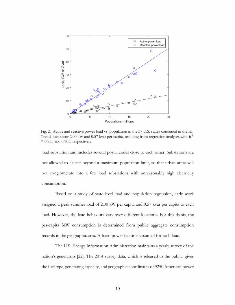
10

load substation and includes several postal codes close to each other. Substations are

not allowed to cluster beyond a maximum population limit, so that urban areas will

not conglomerate into a few load substations with unreasonably high electricity

consumption.

Based on a study of state-level load and population regression, early work

assigned a peak summer load of 2.00 kW per capita and 0.57 kvar per capita to each

load. However, the load behaviors vary over different locations. For this thesis, the

per-capita MW consumption is determined from public aggregate consumption

records in the geographic area. A fixed power factor is assumed for each load.

The U.S. Energy Information Administration maintains a yearly survey of the

nation’s generators [22]. The 2014 survey data, which is released to the public, gives

the fuel type, generating capacity, and geographic coordinates of 9250 American power

Fig. 2. Active and reactive power load vs. population in the 37 U.S. states contained in the EI.

Trend lines show 2.00 kW and 0.57 kvar per capita, resulting from regression analyses with 𝑅2 = 0.935 and 0.903, respectively.

11

plants. In building fictitious cases, we place generation substations at the reported geo-

graphic locations of these actual generators, with generation limits as given. Based on

the fuel type and generation capacity, we estimate the generator’s capability curve and

add corresponding reactive power limits with a linear approximation, as shown in

Table 1.

From the clustered population data, a certain percentage of load substations

are randomly selected as substations with both generators and loads, whereas the

remaining load substations will only contain loads. This thesis uses the load MW to

randomly pick a gen-load ratio value for each of the selected substations. Then, all

available power plants are sorted and assigned to a substation in the increasing order

of their distances to it until this substation satisfies its minimum generation capacity

requirement. In the created synthetic network, only conventional coal- and gas-fueled

power plants are allowed to be located in the same substations with loads.

The remaining power plants are clustered into substations with only generators

in a similar way to the postal code grouping. An additional constraint is enforced such

that any hydro, nuclear or renewable energy resource cannot be grouped together with

a power plant of a different fuel type.

TABLE 1 GENERATOR PARAMETERS

Governor Type

Max Mvar as fraction of MW capacity

Min Mvar as fraction of MW capacity

Steam 0.466 -0.122 Gas 0.509 -0.111 Gas Turbine 0.560 -0.164 Hydro 0.384 -0.049 Nuclear 0.368 -0.082 Wind 0.213 -0.144

12

Throughout this thesis, two example test cases are discussed as each step of

the network synthesis process is illustrated. The first is a 150-bus test case, presented

in [17] with a simplified algorithm. This case uses the geographic footprint of the U.S.

state of Tennessee, which covers approximately 35° N to 36.5° N latitude and 90°

W to 82° W longitude. It was originally designed for the analysis of geomagnetically

induced currents (GIC), a topic discussed in a later chapter, coupled with the standard

ac power flow analysis. This model is publicly available online [23].

The substation placement process for the 150-bus case was performed as

follows. We clustered the 276 generation units publicly reported for Tennessee into 27

equivalent units located at 8 substations. Each generating unit will then have a total

maximum MW generating capacity and fuel type, both of which are public infor-

mation. These are used to assign reactive power limits according to Table 1. We also

add generator step-up transformers, which are important to GIC calculations, from an

assumed generation voltage of 13.8 kV to the substation main bus. For load, the

clustering process groups the state’s 989 zip code tabulation areas into 90 clusters.

Each cluster becomes a load substation with a load value based on the total population

of the postal codes in the cluster. The result of this step is a set of 90 load substations

and 8 generating substations, with geographic coordinates, load, generation parameters,

and grounding resistance already assigned.

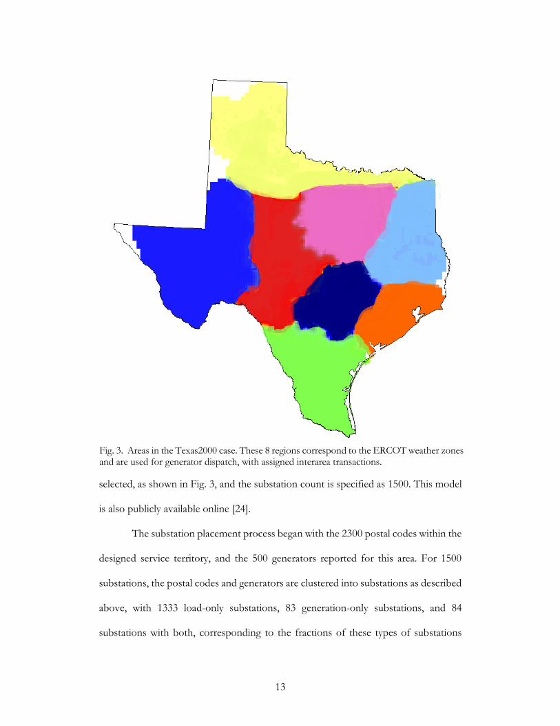
The second test case this thesis describes is the 2000-bus test case from [18],

known as the Texas2000 case, which uses a more complex algorithm for the larger

footprint of the part of the U.S. state of Texas served by the Electric Reliability Council

of Texas (ERCOT), which comprises most of the state. Eight geographic areas are

13

selected, as shown in Fig. 3, and the substation count is specified as 1500. This model

is also publicly available online [24].

The substation placement process began with the 2300 postal codes within the

designed service territory, and the 500 generators reported for this area. For 1500

substations, the postal codes and generators are clustered into substations as described

above, with 1333 load-only substations, 83 generation-only substations, and 84

substations with both, corresponding to the fractions of these types of substations

Fig. 3. Areas in the Texas2000 case. These 8 regions correspond to the ERCOT weather zones and are used for generator dispatch, with assigned interarea transactions.

14

found in real cases. For each substation, an area-dependent power consumption per

capita is assigned, as shown in Table 2, with the total system load of 49,776 MW. Load

power factor is fixed at 0.96. By area, generators are given an initial dispatch

proportional to load. Fig. 4 shows the substations in the Texas2000 case.

TABLE 2 POWER CONSUMPTION PER CAPITA BY AREA

Area

Per-capita

consumption,

kW

Area Per-capita

consumption, kW

COAST 2.362 NORTH 1.859

EAST 1.563 SCENT 2.045

FWEST 1.854 SOUTH 1.843

NCENT 2.438 WEST 2.368

15

Fig. 4. Substations in the Texas2000 case. Red substations are 345 kV; gray substations are 115 kV. The density of substations mirrors population density, as the load is taken from U.S. Census data.

16

Chapter 4: Buses, Transformers, and Transmission Lines

Next, the substations are connected with a synthetic bus-branch topology at

multiple nominal voltage levels. For the approach of this thesis, each substation already

has load, generation, and geographic coordinates determined from the previous step,

and this data is available and used as the buses, transformers, and transmission lines

are generated.

The network designer will select one or more nominal voltage levels for the

synthetic network. It is typical to have 2-3 main system levels for a case with only a

thousand buses or so, usually one extra-high voltage level such as 345 kV, 500 kV, or

765 kV, and another lower voltage level such as 115 kV, 138 kV, 161 kV, or 230 kV.

Cases with tens of thousands of buses will have many more voltage levels, some

spanning multiple areas and possibly a few that span the entire case. For the 150-bus

case, the levels were chosen to be 230 kV and 500 kV, while the Texas2000 case were

assigned the levels 115 kV and 345 kV.

Most substations will contain buses at the lowest level, and a percentage of the

substations will also contain a bus at higher voltage levels. The nominal voltage level

17

selection and percentage of substations containing buses at each level vary widely

among real power systems, and so these will often be chosen according to the desired

characteristics of a synthetic network. Typically, 10-20% of substations contain a bus

at a higher system voltage level, and these may be chosen randomly with probabilities

proportional to load. Large generating substations are significantly more likely to be at

a higher voltage level as well. Transformers are added within substations to connect

the nominal voltage levels. A substation’s loads are usually connected to the lowest

voltage level, and the generators are often connected to the highest voltage level at a

substation, through a step-up transformer. An example substation one-line diagram is

shown in Fig. 5 from the Texas2000 case.

Fig. 5. A sample substation from the Texas2000 case, showing the generator, step-up transformer to the 345 kV bus, and two parallel transformers stepping down to the 115 kV bus at this substation. Three transmission lines connect the 345 kV bus to other substations.

18

Once the substations are assigned buses at various nominal voltage levels,

these voltage levels are connected with a set of transmission lines. The rest of this

chapter discusses the development of transmission line parameters; the topology will

be explained in the next chapter.

Transmission line electrical parameters required for ac power flow analysis

include series impedance, shunt admittance, and MVA limits. Realistic per-distance

parameters are assigned to synthetic lines based on datasheets and references,

appropriate to the assigned nominal voltage level 𝑉𝑙𝑖𝑛𝑒, for both overhead lines and

underground cables. For the line length 𝑙 , the straight line distance between the

assigned substation geographic coordinates is used. The actual right-of-way distance

for a real transmission line is always longer than this, but the point-to-point distance

suffices as an approximation.

The majority of actual lines in the transmission system are overhead lines, and

therefore most synthetic lines are assigned parameters realistic to overhead lines. In

building synthetic overhead lines, first, a few candidate conductor types are selected

typical to the assigned nominal voltage level, following the conventions of [25]. Data

for each conductor includes outer radius 𝑟𝑜, geometric mean radius 𝑟′, per-distance

resistance 𝑟 at 50°C, and the maximum current carrying capacity 𝐼max. Transmission

line capacities can be improved with conductor bundling, and this is common at higher

voltage levels such as 345 kV and 500 kV. Synthetic lines at these voltage levels are

given bundled conductors with 𝑏 conductors per bundle, spaced at 18 inches. The

final selection of conductor from the realistic choices is made based on estimated

capacity requirements, as determined by the dc power flow the next chapter will

describe. For the assigned voltage level, a list of candidate transmission tower

19

configurations is also created using the variety of towers found in [26], [27]. One tower

style is randomly selected for each line from the realistic candidates at that voltage

level. From the tower data, the geometric mean distance 𝐺𝑀𝐷 between phases is

calculated, depending on the arrangement of the lines on the tower.

The overhead line parameters 𝑅, 𝑋, 𝐵, and 𝑀𝑉𝐴max are calculated as follows

[25]-[27]: 𝑓 is the system frequency, 60 Hz for North America, and 𝜖 is the permittivity

of free space, 1.42461 × 10−8 𝐹

𝑚𝑖. For bundled conductors, 𝑟′ and 𝑟𝑜 will be replaced

by equivalent bundle spacing values 𝐷𝑆𝐿 and 𝐷𝑆𝐶 .

𝑅 =

𝑟 × 𝑙

𝑏 (1)

𝑋 = 2𝜋𝑓 × 0.0003218 × 𝑙𝑛 (

𝐺𝑀𝐷

𝑟′) × 𝑙 (2)

𝐵 = 2𝜋𝑓 × (2𝜋𝜀

ln (𝐺𝑀𝐷

𝑟𝑜)

× 𝑙)

−1

(3)

𝑀𝑉𝐴𝑚𝑎𝑥 = √3 × 𝐼𝑚𝑎𝑥 × 𝑉𝑙𝑖𝑛𝑒 × 𝑏 (4)

An example 345 kV transmission tower diagram is shown in Fig. 6, and Fig. 7 shows

the long-line transmission model used for transmission lines in power system analysis.

Underground transmission lines are less common due to their high cost, but

are sometimes used in urban settings where overhead right of ways are costly,

unavailable, or are aesthetically problematic [28]. They are distinguished from

overhead lines in their lower series impedance and much higher shunt charging

admittance due to the tight bundling of the phase conductors. A few synthetic lines

are assigned parameters as underground cables if their distance is short and they have

a large load at either end, characteristics of a metropolitan setting. Similar to the

overhead lines, a set of candidate conductors and cable configurations is derived from

20

reference manuals [29], [30] for the associated voltage level. All cables are assumed to

be cross-linked polyethylene (XLPE), also known as solid dielectric cables. Two cable

material types are considered – copper conductor with lead sheath and aluminum

conductor with aluminum sheath – and three conductor sizes for each material type.

The final choice for conductor depends on the estimated capacity needed, and there

Fig. 6. 345 kV transmission tower, with phase spacing, D, of 24 ft [26].

Fig. 7. Long-line transmission line model [25].

21

is some randomization in the cable configuration. 75% of synthetic cables are

configured to be pulled in a duct, while the rest are directly buried in the dirt [28]. Both

installations assume earthing at a single point and a trefoil phase layout. Line

parameters are calculated with equations similar to (1)–(4).

22

Chapter 5: Network Topology and the Delaunay Triangulation

An automated line placement process is necessary to build large synthetic

systems in reasonable time. The approach of this thesis is to match a set of network

properties which characterize the network’s graph topology, geometry, and power flow

solution. These quantitative metrics can be used for building synthetic networks as

well as for validation criteria of created networks. A brief discussion of some basic

topological criteria follows.

The approach of this thesis is to build a connected graph at each voltage level,

and for the combined graph at all voltage levels to remain connected even if one

substation is removed. This property does not allow for radial substations and

enhances contingency behavior.

This thesis proposes an algorithm which adds lines for all voltage level

networks at the same time, iteratively inserting lines at each nominal voltage level. A

penalty-based system is used to rank the candidate lines during the selection process.

As long as the connectivity requirements mentioned above are not yet met, heavy

penalties are given to candidate lines which do not contribute to connectivity under a

23

single node removal. These penalties dominate the early part of the line placement

algorithm until these topological criteria are satisfied. The other properties described

increase the intelligence of the line selection process by adding other penalties, so that

the final network will be more realistic and match multiple properties found on real

power systems.

For a general transmission network at a single nominal voltage level, 𝑛

substations are connected with 𝑚 transmission lines. The topology of these

transmission lines can be expressed with the symmetric adjacency matrix 𝐴, where

𝐴(𝑖, 𝑗) = {

1, if a line exists from 𝑖 to 𝑗 0, else

(5)

𝑖, 𝑗 ∈ {1, 2, … , 𝑛} .

Node degree 𝑘𝑖 for node 𝑖 indicates the number of edges incident on that

node.

𝑘𝑖 = ∑ 𝐴(𝑖, 𝑗)

𝑛

𝑗=1

(6)

The average nodal degree is

⟨𝑘⟩ =

1

𝑛∑ 𝑘𝑖

𝑛

𝑖=1

=2𝑚

𝑛 . (7)

The Eastern Interconnect (EI) networks show a highly linear relationship

between 2𝑚 and 𝑛; the correlation coefficient is 0.9991. This indicates an average

nodal degree of 2.43, consistent across networks of various sizes and voltage levels.

This number fits the range of results found in other studies [6], [11]. From the average

nodal degree, the number of transmission lines in a network 𝑚 will be 1.22𝑛 ,

according to (7).

24

The distribution of node degrees across a system is another common indicator

of network structure. The internet, social networks, and some biological networks have

a power-law scale-free node degree distribution [10]. In contrast, power system

networks lack central hubs with a large degree, and have consistently been shown to

have an exponential node degree distribution, defined by

Pr(𝑘) = 𝛼𝑒−𝛽𝑘 , (8)

for some constants 𝛼 and 𝛽, which is confirmed in Fig. 8 for the 28 networks studied

with 𝑛 > 100 , using 𝛼 = 1.19 and 𝛽 = 0.69 . The exponential node degree

distribution reflects the geographic constraints which dominate the careful planning

of power networks. We observe that transmission networks consistently deviate from

the exponential distribution with 𝑘 = 1 and 𝑘 = 2. This property has been noted by

Fig. 8. Node degree distribution for 28 of the single-voltage transmission networks on the EI

with 𝑛 > 100, and exponential regression for 𝑘 ∈ [3, 7]. Thin vertical lines are range, thicker lines are inner quartiles, horizontal dash shows the median, and the crosses show outliers.

25

previous studies [6], [11], and reflects the planning priority to avoid substations relying

on a single line for service.

The average shortest path length, ⟨𝑙⟩, denotes how many hops along the edges

of a network separate two nodes, on average. It can be calculated from a network’s

adjacency matrix 𝐴 using Dijkstra’s algorithm [31]. A purely random network, defined

by a set of nodes in which each pair is connected with probability 𝑝, will have ⟨𝑙⟩

which scales logarithmically with n [8]

⟨𝑙⟩𝑟𝑎𝑛𝑑 ≈

ln(𝑛)

ln(⟨𝑘⟩) . (9)

This is the small world property: even in very large networks, most nodes are

only a few hops apart. On the other hand, regular lattice networks have much larger

average path lengths, scaling with a 1/𝑑 power law, where 𝑑 is the dimension of the

lattice. So two-dimensional lattices will have

⟨𝑙⟩2𝐷 ∝ √𝑛 . (10)

Small World networks, as presented in [5] and compared to the power system

by many [6]–[8], [10]–[11], retain the logarithmic scaling property of random networks.

Figure 9 shows the average shortest path length calculations for the 94

transmission networks surveyed from the EI. It can be seen that when transmission

networks are considered using each voltage level independently, the logarithmic scaling

property for average shortest path length is not seen, and the network approximates a

regular two-dimensional lattice. Reference [7] also observes a difference between the

scaling properties of power systems’ average shortest path length and that of Small

World networks. The shortcuts mentioned in other previous work [11] reflect the

26

superposition of multiple voltage levels, but these levels individually appear to be more

accurately approximated by lattices.

The average clustering coefficient, ⟨𝑐⟩, is the second primary indicator of a

small world. An individual node with node degree 𝑘𝑖 has 𝜏𝑖 possible edges

interconnecting its neighbors, where

𝜏𝑖 =

𝑘𝑖(𝑘𝑖 − 1)

2 . (11)

The clustering coefficient for a node 𝑐𝑖 is defined by

𝑐𝑖 =

𝑒𝑖

𝜏𝑖 , (12)

Fig. 9. Average shortest path length ⟨𝑙⟩ for 94 single-voltage transmission networks on the EI, compared to expected scaling properties for random graph and 1D, 2D, and 3D regular lattices.

27

where 𝑒𝑖 is the number of edges actually interconnecting node 𝑖’s neighbors. ⟨𝑐⟩ is the

average of 𝑐𝑖 over all nodes in the network. For completely random networks the value

⟨𝑐⟩ is given by

⟨𝑐⟩𝑟𝑎𝑛𝑑 ≈

⟨𝑘⟩

𝑛 . (13)

Clustering in truly random networks therefore decreases rapidly with system

size [8]. Regular lattices, in contrast, have much larger clustering coefficients that do

not scale with system size [5]. Small World networks approximate the clustering

coefficient properties of a lattice, while maintaining the average shortest path length

of a random network [5], [8]. In general, the 94 transmission networks studied show a

large clustering coefficient uncorrelated to network size, as expected for a Small World

network or regular lattice. The average ⟨𝑐⟩ among the networks is 7.5%, but the value

varies significantly. Many small networks have so few edges that either no clustering

appears or the clustering is quite high. For networks with more than 100 substation

nodes, ⟨𝑐⟩ falls consistently in the range 1%-15%, much higher than for a random

network.

Because our approach begins by giving each substation node latitude and

longitude coordinates, this additional information is available for building the synthetic

topologies. From computational geometry, the Delaunay triangulation for a set of

points is a simple planar mesh that connects 𝑛 points with non-overlapping line

segments, dividing the region into triangles. The Delaunay triangulation is

distinguished from a general triangulation by the property that no triangle has a point

inside its circumcircle, and the smallest angle is maximized [32], [33]. The triangles are

therefore nicely shaped; when possible they have all acute angles. A node’s neighbors

28

on the Delaunay triangulation will also be the nodes nearest to it by geometric distance.

Figure 10 illustrates the Delaunay triangulation.

From graph theory, Euler’s formula states for a planar graph such as the

Delaunay triangulation, with 𝑛 points, 𝑚 edges, and 𝑓 faces [31],

𝑛 − 𝑚 + 𝑓 = 2 . (14)

Since in the Delaunay triangulation each face is a triangle except the region

outside the graph,

3(𝑓 − 1) + 𝑝 = 2𝑚 , (15)

where 𝑝 is the number of edges on the outer boundary of the graph. Substituting for

𝑓 and solving for 𝑚, we get

𝑚 = 3𝑛 − 𝑝 − 3 . (16)

Fig. 10. Triangulation of a set of 5 points. (a) is not the Delaunay triangulation, because at least one triangle’s circumcircle contains another point. (b) is the Delaunay triangulation of these points, because no triangle’s circumcircle contains another point. Note that there are both larger and smaller angles in (a) than in (b).

29

So a large Delaunay triangulation will have about 3𝑛 edges, since 𝑝 will be

small with respect to 𝑛. Therefore the average nodal degree ⟨𝑘⟩ will be 6 regardless of

system size [32]. A Delaunay triangulation on points uniformly distributed

approximates a two-dimensional regular lattice, with a constant clustering coefficient

of 40%, and an average shortest path length of √𝑛, where 𝑛 is the number of points

[33].

Because Delaunay matches these basic properties found in real power systems

and connects nodes with geometric proximity, it provides a reasonable subject for

direct comparison to real grids. Each actual transmission line in these single-voltage

networks has a Delaunay separation, indicating the shortest distance between the line’s

Fig. 11. Separation of transmission line endpoints on the Delaunay triangulation, in hops, for 94 single-voltage transmission networks on the Eastern Interconnect. Thin vertical lines are the range; thicker lines are inner quartiles; horizontal dash shows the median; and the crosses show outliers.

30

endpoints along the segments of the substations’ Delaunay triangulation. A separation

of 1 means the line is itself one of the segments of the Delaunay triangulation; a

separation of 2 means a path of two Delaunay segments connects the line’s endpoints.

The results are plotted in Fig. 11. The Delaunay triangulation contains 70% of an

average network. This is significant since there are 𝑛(𝑛 − 1) possible transmission

lines, 1.22𝑛 actual transmission lines, and 3𝑛 segments on the Delaunay triangulation.

The actual lines that are not on the Delaunay triangulation are nearly all only a few

hops separated. 98% of lines in the average network have a Delaunay separation of 3

or less. A substation’s Delaunay neighbors are also its closest neighbors by geometric

distance, so this property reflects the geographic constraints of transmission system

planning.

For the graphs of transmission line networks of various utilities in the Eastern

and Western interconnects in North America, the transmission lines connect

geographically located substations. A comparison was made for each real transmission

line to the Delaunay triangulation of the substations at that voltage level. Table 3 shows

the results averaged over 28 Eastern networks and 15 Western networks, each over

TABLE 3 CORRELATION BETWEEN DELAUNAY TRIANGULATION

AND ACTUAL TRANSMISSION LINES

Transmission Line Category

Average percentage for

Eastern Interconnect

Average percentage for

Western Interconnect

Minimum Spanning Tree 47.8% 44.3%

Delaunay Triangulation 75.6% 71.1%

Delaunay 2 neighbor 18.3% 21.5%

Delaunay 3 neighbor 4.6% 5.3%

Delaunay 4 neighbor 1.1% 1.4%

Delaunay 5+ neighbor 0.4% 0.7%

31

100 kV with more than 80 substation nodes. The percentages indicate how many

transmission lines fall on the minimum spanning tree or Delaunay triangulation. For

those that fall on neither, the neighbor distance is given along the segments of the

Delaunay triangulation. For a line that is a Delaunay 3 neighbor, the shortest path

between the line endpoints along the Delaunay triangulation is three segments. The

minimum spanning tree segments are also on the Delaunay triangulation. This shows

that overlap with the Delaunay triangulation and its near neighbors is a good indicator

of real power systems.

A synthetic power system’s correlation with the Delaunay triangulation at each

voltage level can be an important indicator of how realistic the transmission line

topology is. It can easily be integrated into the penalty-based iterative line placement

algorithm by setting a quota of lines which may be added from each category:

minimum spanning tree, Delaunay, Delaunay 2 neighbor, and so forth. To ensure

adequate progress toward the quotas, during the line placement process penalties are

added to candidate lines in categories that exceed the proportion allowed. Each

nominal voltage level will have its own set of Delaunay categories with its own set of

quotas.

In fact, using the Delaunay triangulation can be a great aid to building synthetic

transmission line topologies. There are approximately 𝑛2 possible lines connecting a

set of 𝑛 substations. Restricting candidate lines to the Delaunay 3 neighbors and closer

cuts the number down to about 23𝑛, dramatically reducing the number of candidate

lines to analyze, especially for networks with more than 1000 substations. This first-

level pruning eliminates many candidate transmission lines which are statistically very

unlikely due to geographic constraints.

32

Real power system models have convergent ac power flow solutions. Using a

dc power flow solution as part of the iterative line placement algorithm can increase

the solvability of cases, since lines are placed in locations that facilitate connecting

generation with load. Figure 12 illustrates how the voltage angle gradients are related

to real power flows in a typical transmission system. The standard dc power flow [34]

solves for a vector of system bus voltage angles, 𝜽, with known real power injection

𝑷𝒊𝒏𝒋 and system susceptance matrix 𝑩. It is solved as

𝜽 = −𝑩−1𝑷𝒊𝒏𝒋 . (17)

As long as the system is connected, meaning 𝑩 is not a singular matrix, the dc

power flow will have a solution. Any candidate line can then have an estimated power

flow value 𝑃𝑒𝑠𝑡, provided the line length and per-distance impedance 𝑑21 and 𝑥𝑙 are

known:

𝑃𝑒𝑠𝑡 = 𝑥𝑙 ⋅ 𝑑21 ⋅ (𝜃2 − 𝜃1) (18)

Fig. 12. Contour of voltage angles, showing gradient where addition of transmission line could be beneficial.

33

where 𝜃1 and 𝜃2 are the voltage angles of the buses this line would connect. A negative

penalty is given to candidate lines, proportional to 𝑃𝑒𝑠𝑡. This incentivizes power flow

corridors in the automatic line placement algorithm, subject to the other system

constraints.

To ensure a connected network before enough transmission lines have been

added, the dc power flow step adds an additional set of temporary impedances

corresponding to lines forming the substations’ Euclidian minimum spanning tree.

These impedances are in addition to the actual transmission lines as they are added,

and the impedance magnitudes are increased throughout the line placement process

until the graph is connected by actual transmission lines, at which point these

temporary impedances will be removed. The temporary impedances serve to connect

the graph while the in-progress transmission line topology is still disconnected,

allowing dc power flow solutions even in the earliest stages.

Sometimes, two transmission lines of the same voltage level will intersect, or

pass by one another, external to a substation. These can be found by simple geometry

if the substation coordinates are known at the line endpoints. If all the lines come from

the Delaunay triangulation, there can be no intersections. However, matching the 2

neighbors and 3 neighbors of the Delaunay triangulation, as is done in this thesis,

allows for lines to intersect one another.

An analysis of line intersections in high-voltage networks of the Eastern and

Western Interconnects in North America indicates that line intersections do occur, but

they are uncommon, especially for higher voltage levels. The line algorithm will often

intrinsically produce line intersection rates larger than what is realistically seen, so a

34

penalty is added to candidate lines that intersect existing lines, so that the intersection

rate can be made to match that of actual cases.

In the 150-bus case, all 98 substations are given a 230 kV bus, and the largest

18 load and 7 generation substations are given a 500 kV bus. The transmission line

topologies at each nominal voltage level are built by adding 1.22n transmission lines,

which are all selected from the 3n lines of the Delaunay triangulation. We begin with

the Euclidian minimum spanning tree at each voltage level, guaranteed to be a subset

of the Delaunay triangulation. This ensures a connected graph, and reflects the

geographic constraints of real power systems. Then about 0.22n lines will be added in

an iterative fashion, all taken from the 3n segments of the substations’ Delaunay

triangulation. The expected properties ⟨l⟩ and ⟨c⟩ follow the scaling behaviors for the

regular lattice of which they are a subset. These additional lines will be selected from

a dc power-flow based metric.

The result is a set of 121 synthetic transmission lines at 230 kV and 30 lines at

500 kV, with per-distance parameters according to Table 4, connecting the 98 synthetic

substations across the geographic area. The statistical data from this 150-bus case is

shown in Table 5. Because the number of transmission lines is directly controlled, the

average nodal degree ⟨k⟩ is very close to the target 2.43 for both networks. With the

TABLE 4 LINE PARAMETERS USED BY THE 150-BUS CASE

kV ACSR

Conductor Tower spacing

Per-unit impedance, per 100 miles

MVA limit

x r b

500 Falcon, 3 bundle

42 ft. 0.00193 0.000912 2.126 3585

230 Cardinal, 1 bundle

24 ft. 0.15186 0.021323 0.278 402

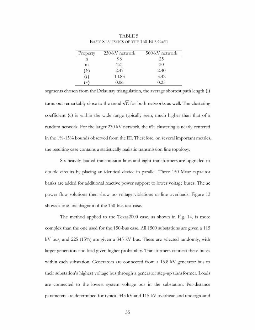
35

segments chosen from the Delaunay triangulation, the average shortest path length ⟨l⟩

turns out remarkably close to the trend √𝑛 for both networks as well. The clustering

coefficient ⟨c⟩ is within the wide range typically seen, much higher than that of a

random network. For the larger 230 kV network, the 6% clustering is nearly centered

in the 1%-15% bounds observed from the EI. Therefore, on several important metrics,

the resulting case contains a statistically realistic transmission line topology.

Six heavily-loaded transmission lines and eight transformers are upgraded to

double circuits by placing an identical device in parallel. Three 150 Mvar capacitor

banks are added for additional reactive power support to lower voltage buses. The ac

power flow solutions then show no voltage violations or line overloads. Figure 13

shows a one-line diagram of the 150-bus test case.

The method applied to the Texas2000 case, as shown in Fig. 14, is more

complex than the one used for the 150-bus case. All 1500 substations are given a 115

kV bus, and 225 (15%) are given a 345 kV bus. These are selected randomly, with

larger generators and load given higher probability. Transformers connect these buses

within each substation. Generators are connected from a 13.8 kV generator bus to

their substation’s highest voltage bus through a generator step-up transformer. Loads

are connected to the lowest system voltage bus in the substation. Per-distance

parameters are determined for typical 345 kV and 115 kV overhead and underground

TABLE 5 BASIC STATISTICS OF THE 150-BUS CASE

Property 230-kV network 500-kV network

n 98 25 m 121 30

⟨𝑘⟩ 2.47 2.40

⟨𝑙⟩ 10.83 5.42

⟨𝑐⟩ 0.06 0.25

36

transmission lines, with several variations and conductor upgrades. Lines which are

shorter than 8 miles and connect at least 200 MW of load are considered underground.

The transmission line placement process adds 287 lines at 345 kV and 1813

lines at 115 kV. Of these lines, 231 are added as double circuits, 42 are added as triple

circuits, and 22 are added as quadruple circuits. The lines are all added from the set of

line segments including the Delaunay triangulation and any pair of substations

separated by three or fewer Delaunay segments, as opposed to the 150-bus case which

merely added lines from the Delaunay triangulation. At each of 420 iterations, each of

Fig. 13. Geographic single-line diagram of 150-bus test case.

Fig. 14. Flowchart of network synthesis process.

37

these candidate lines is ranked according to a set of penalties as shown in Table 6,

corresponding to the observations of this chapter, and the five highest-ranked

segments are added to the network. Based on the dc power flow results, conductors

were selected for transmission lines, and some lines were upgraded to multiple circuits.

Figure 15 shows the lines added to the Texas2000 case. The computation time for

building the line topology of this case was about 5 minutes.

The synthetic network has no relation to the actual grid in Texas, except that

the load and generation profiles are similar. The transmission line topology meets

validation criteria described before in the form of structural statistics gathered from

the Eastern Interconnect. The combined graph of both voltage levels is fully

connected and remains so under a single node removal. Each individual voltage level

network is fully connected. The number of transmission lines in proportion to the

number of substations is close to the 1.22 target for both networks. Table 7 shows

structural statistics for this case, including the proportion of lines at each voltage level

TABLE 6 PENALTY STRUCTURE FOR LINE PLACEMENT IN 2000 BUS CASE

Criterion Amount of penalty for each candidate line segment

Distance +2 per mile

Power Flow -0.5 × 𝑃𝑒𝑠𝑡 based on (7)

Category +200 if ahead of quota for the segment’s category: minimum spanning tree, Delaunay triangulation, or 2 or 3 neighbor of the Delaunay triangulation

Voltage level connectivity

-300 if segment contributes to connectivity at single voltage level, or connects to a radial substation

Overall connectivity

-1000 if segment contributes to full system connectivity under single node removal

Intersections +500 if segment intersects with existing line

38

which are from the substations’ minimum spanning tree, Delaunay triangulation, and

the Delaunay neighbors with distance 2 and 3. Comparing these proportions to those

from Table 3 shows that the proportions of each category are close to target. Table 7

also shows the line intersection rate, which the intersection penalty has brought below

the maximum thresholds normally seen in actual cases.

The resulting case has an ac power flow solution without any manual

intervention. Some low-voltage areas benefit from 36 manually added shunt capacitor

banks. The generator setpoints were modified manually as well for some units, and

Fig. 15. Transmission lines added to the Texas2000 case. The red lines are 345 kV, and the gray lines are 115 kV.

39

five shunt reactors were added in areas that had overvoltages. For a case of this size,

manually adding reactive power support is possible, but future work will address this

problem for larger cases in a more systematic way. The final case has no lines loaded

more than 85%, nor voltages outside of the 0.97-1.05 per-unit range. Figure 16 shows

the ac power flow solution with the system voltage profile contour [35].

TABLE 7

STRUCTURAL STATISTICS OF THE TEXAS2000 CASE

Structural Statistic Target Quota

345-kV network

115-kV network

𝑛 - - 225 1500

𝑚 - - 287 1813

𝑚/𝑛 1.22 1.276 1.209

Minimum spanning tree 50% 49.1% 50.6% Delaunay Triangulation 70% 69.7% 70.9% Delaunay 2 neighbor 25% 24.7% 24.7% Delaunay 3 neighbor 5% 5.6% 4.4% Line intersections < 20% 6.5% 9.1%

40

Fig. 16. Voltage profile contour of the Texas2000 case.

41

Chapter 6: Application to Geomagnetic Disturbance (GMD) Analysis

Simulation and analysis of geomagnetic disturbances (GMDs) are an im-

portant part of building more resilient electric power transmission systems. GMDs

occur when solar activity such as earth-directed coronal mass ejections or solar coronal

holes causes variations in the earth’s magnetic field. Resulting geomagnetically induced

currents (GICs) tend to flow through low resistance paths such as transmission lines,

connected to earth at grounded substations through transformer neutrals. From a 60

Hz grid perspective, GICs can be deemed as “quasi-dc” (less than 1 Hz), superimposed

on the predominantly ac grid. Sufficiently large GICs may cause half-cycle saturation

in transformers and damage them; more likely, GICs may lead to relay mis-operation,

the tripping of reactive power support devices, and voltage collapse in the grid [36].

To evaluate the threats a major GMD would pose to the power system and

the mitigation measures needed to operate the grid safely, the Federal Energy

Regulatory Commission (FERC) in Order 797 directed the North American Electric

Reliability Corporation (NERC) to develop standards for planning and operating the

grid under GMDs [37]. System studies proposed in NERC’s planning standards [38]

42

will require specialized planning tools and modeling capabilities. Methodologies for

modeling GMDs for large power system studies are given in [39]. GMD studies need

particular inputs such as substation grounding resistances and geographic coordinates

for electric field calculations, so the typical IEEE transmission system test cases are

not sufficient. The 17-bus case of [40] is one test case designed for GIC calculations;

it models a version of the Finnish 400-kV grid with dc resistances given for substation

grounding and transmission lines. The 20-bus dc case of [41] models two voltage levels

and adds transformer dc resistance values. These cases do not include the ac power

flow parameters necessary to couple GIC calculations into a steady-state voltage

stability analysis of the power system under a GMD, as [39] describes and the NERC

standards [38] propose. Existing larger and more detailed cases of the actual grid

contain critical infrastructure information and are subject to data confidentiality,

restricting their use for public validation of GMD analysis methodologies. The

development of larger public test cases with more detail, including both dc and ac

parameters, will aid research on this topic and allow for cross-validating software and

analysis methods.

Though not always included in standard power system models, geographic

coordinates are critical for GMD analysis. Therefore, the methodology presented in

this thesis is well-suited to GMD applications, by augmenting synthetic cases with

other parameters this analysis needs. As a benchmark, representative GMD study

results for the 150-bus case are provided in this chapter, following the GIC calculation

methodology of [39].

Current planning models and IEEE test cases do not contain substation

grounding data, since they are not used in standard power flow studies [39]. The

43

typically observed range of this parameter is 0.015 to 1.5 Ω [42], [43]; previous work

has shown that GIC results are quite sensitive to these values and that actual values

should be used wherever possible [42]. In this method, each substation has a grounding

resistance assigned based on the assumed size of the substation, considering the

nominal voltage level and the number of buses in a substation. Table 8 shows the

substation grounding used in this case.

Several transformer parameters not used in power flow analysis, which are

essential to GMD studies, are included in the model. Table 9 summarizes these

parameters for the 60 transformers in the case; the full data is available at [23]. The

winding resistances were estimated from the ac series resistance values of the

transformers using the methodology described in [39]. Note that the low side winding

resistances for the GSUs have not been given, due to the delta connection on the low

TABLE 8 SUBSTATION DATA SUMMARY

Maximum Nominal Voltage (kV) ↓

Generating Non-generating

Number of Substations

Grounding Resistance

(Ohm)

Number of Substations

Grounding Resistance

(Ohm)

500 7 0.11 – 0.15 18 0.18 230 1 0.38 72 0.47

TABLE 9 TRANSFORMER DATA SUMMARY

Nominal Voltage

(kV)

Number of Trans-formers

Type Winding Config.

Winding Resistance, Ω

𝐾 High (Series)

Low (Common)

500-230 33 Auto GWye- GWye-

0.2500 0.1841 1.8

500-13.8 26 GSU GWye-Delta

0.153 – 1.3554

N/A 1.8

230-13.8 1 GSU GWye-Delta

1.4469 N/A 1.5

44

side, which does not provide a path to ground for the GICs. In the last column, the 𝐾

values relate the transformer effective GICs to reactive power losses according to the

following expression derived from [44]:

𝑄loss,pu = 𝑉pu𝐾𝐼GIC,pu, (19)

TABLE 10 TRANSFORMER GIC RESULTS

HV Bus #

LV Bus #

𝐼𝑛 (Amps)

𝐼GIC (Amps)

HV Bus #

LV Bus #

𝐼𝑛 (Amps)

𝐼GIC (Amps)

92 63 19.536 8.111 139 123 -19.038 6.346 93 54 7.111 1.609 139 138c1 -7.824 3.411 94 40 1.274 5.169 139 138c2 -7.824 3.411 95 86 -42.335 13.332 140 135 -8.982 2.994 96 23 -11.798 5.805 142 110 19.558 6.519 97 43 97.751 32.504 142 111 13.004 4.335 98 11 -24.757 3.661 142 112 36.911 12.304 99 79ck1 -67.529 20.723 142 141c1 21.610 6.933 99 79ck2 -67.529 20.723 142 141c2 21.610 6.933 100 64 13.283 3.928 144 1 -42.354 14.118 101 22ck1 18.977 5.189 144 116 -14.083 4.694 101 22ck2 18.977 5.189 144 117 -14.083 4.694 102 8 -13.320 5.415 144 118 -14.083 4.694

103 45 148.57

4 42.687

144 119 -42.354 14.118

104 71 -69.125 18.184 144 143ck1 -10.624 4.907 105 90 38.977 15.403 144 143ck2 -10.624 4.907 106 27 -39.950 19.080 146 130 3.266 1.089 107 33 16.024 0.093 146 131 3.266 1.089 108 14 4.424 7.313 146 132 3.266 1.089 109 49 27.234 8.327 146 133 7.604 2.535 137 124 -9.658 3.219 146 134 7.604 2.535 137 125 -9.658 3.219 146 145c1 8.225 1.109 137 126 -9.658 3.219 146 145c2 8.225 1.109 137 127 -9.658 3.219 148 129 18.192 6.064 137 128 -14.468 4.823 148 147 32.803 12.641 137 136ck1 -17.414 3.603 150 113 6.695 2.232 137 136ck2 -17.414 3.603 150 114 6.695 2.232 139 120 -6.376 2.125 150 115 2.909 0.970 139 121 -6.376 2.125 150 149c1 7.174 2.541 139 122 -19.038 6.346 150 149c2 7.174 2.541

45

where 𝑄loss,pu is the total three-phase reactive losses in a transformer in per unit, 𝑉pu

is the per unit terminal voltage of the high side winding of the transformer, and 𝐼GIC,pu

is the “effective” GIC in the transformer windings. The transformer effective GIC

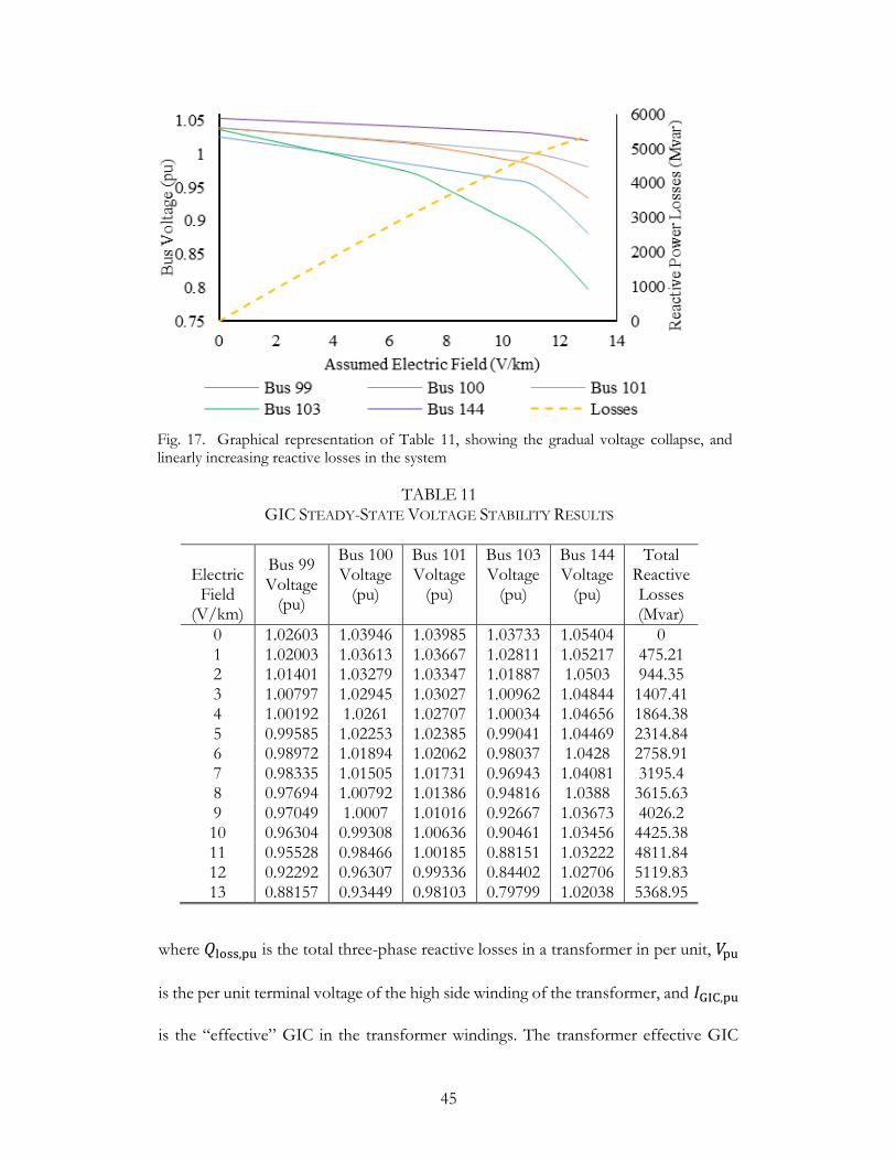
Fig. 17. Graphical representation of Table 11, showing the gradual voltage collapse, and linearly increasing reactive losses in the system

TABLE 11 GIC STEADY-STATE VOLTAGE STABILITY RESULTS

Electric Field

(V/km)

Bus 99 Voltage

(pu)

Bus 100 Voltage

(pu)

Bus 101 Voltage

(pu)

Bus 103 Voltage

(pu)

Bus 144 Voltage

(pu)

Total Reactive Losses (Mvar)

0 1.02603 1.03946 1.03985 1.03733 1.05404 0 1 1.02003 1.03613 1.03667 1.02811 1.05217 475.21 2 1.01401 1.03279 1.03347 1.01887 1.0503 944.35 3 1.00797 1.02945 1.03027 1.00962 1.04844 1407.41 4 1.00192 1.0261 1.02707 1.00034 1.04656 1864.38 5 0.99585 1.02253 1.02385 0.99041 1.04469 2314.84 6 0.98972 1.01894 1.02062 0.98037 1.0428 2758.91 7 0.98335 1.01505 1.01731 0.96943 1.04081 3195.4 8 0.97694 1.00792 1.01386 0.94816 1.0388 3615.63 9 0.97049 1.0007 1.01016 0.92667 1.03673 4026.2 10 0.96304 0.99308 1.00636 0.90461 1.03456 4425.38 11 0.95528 0.98466 1.00185 0.88151 1.03222 4811.84 12 0.92292 0.96307 0.99336 0.84402 1.02706 5119.83 13 0.88157 0.93449 0.98103 0.79799 1.02038 5368.95

46

depends on the winding configuration, and whether the transformer is an

autotransformer or not; its calculation methodology is described in [39]. These losses

are mapped to the power flow model in order to perform ac power flow studies to

study system voltages.

For a 1 V/km, uniform, eastward electric field (𝐸), Table 10 shows the neutral

GIC 𝐼𝑛 in Amperes and the effective GICs 𝐼𝐺𝐼𝐶 in amperes in all of the 60

transformers in the case. The neutral current 𝐼𝑛 is the sum of the neutral current for

all three phases, and is oriented with positive indicating current into the ground.

Transformers highlighted yellow in Table 10 show the highest effective GICs for this

scenario.

The ac power flow data in the case can be used to perform a steady-state

voltage stability study in the presence of GICs. For voltage stability analysis, the

applied electric field, still eastward, is gradually increased in steps of 1 V/km. At each

step, the power flow is solved, and the bus voltages and GIC-induced reactive losses

Fig. 18. 150-bus case bus voltage contours. (Above) Base case. (Below) Voltages at power flow solved with GICs and reactive losses at electric field of 7 V/km

47

of all transformers are noted. This is done until the power flow solution does not

converge. Here the point of non-convergence was reached at 𝐸 = 14 V/km. Table

11 shows bus voltages at select five, 500 kV buses until the last valid power flow

solution, and these values are plotted in Fig. 17, showing gradual voltage collapse in

the system. The detailed numbers in Tables 10 and 11 have been provided to help in

benchmark comparisons. These five buses belong to three major metro areas in

Tennessee, a key junction substation in the case, and one substation near the edge of

the network. Figure 18 shows the voltages contoured at different electric field

strengths to show the impact of the losses on the system voltages. It shows that the

voltages start to fall first near the northeast and southwest edges of the network. Note

that this in no way implies that this response is expected in this footprint for an actual

GMD, as this is a synthetic case. At 𝐸 = 13 V/km there were 49 buses below 0.9 pu

voltage.

48

Chapter 7: Voltage Control, Transient Stability, and Other Future Work

Once a test case has an ac power flow solution with buses, generators, loads,

transformers, and transmission lines, additional complexities can be added to improve

the realism of the case and include data necessary for various types of studies.

Voltage control of real power systems involves a variety of reactive power

compensation and other devices: shunt capacitor banks, transformer taps, static var

compensators, and synchronous condensers. A recent Eastern Interconnect model

contained about 19 000 buses where the voltage was regulated by a device such as a

generator, tap-changing transformer, or switched shunt. Of these, about 1100 devices

regulate a bus other than the one to which they are connected. Over 500 buses are

regulated by multiple devices, with 12 regulated by eight or more devices. Advanced

voltage control methods can be developed in future research to automatically set

generator control buses, control voltages, transformer tap controls, switched shunt

device controls, and phase-shifting devices.

A variety of specialized studies such as transient stability can be done with

added data. An illustrative example of adding transient stability devices would be to

49

model each synthetic synchronous generator with a classical model, as defined in [45],

with parameters for inertia H and transient impedance 𝑋𝑑′ assigned based on a random

distribution for real generators of that fuel type. Further research can expand this

framework to properly configure the dynamic models for realistic synchronous

machines, turbine-governor systems, excitation systems, wind turbines, complex loads,

and system stabilizers.

Other types of specialized studies require additional data. Economic studies

require cost and pricing, which are often quite confidential. Synthetic cases with

realistic cost data can be used for optimal power flow and unit commitment studies.

Reliability studies require more line and generator information about contingency

limits and failure rates, among other information. Each of these specialized

applications can augment the basic set of buses, generators, loads, and branch topology

to meet these particular needs on real geographic footprints with large, realistic, freely-

available test cases.

50

Chapter 8: Discussion and Conclusion

This thesis presents preliminary considerations and a process to generate

synthetic power system test cases. Synthetic networks built with the methodology of

this thesis can equip power systems research with high-quality public test cases which

match the size and complexity of actual grids. Cases created using this method are

synthetic, with no relation to the actual grid in their geographic location; therefore, by

nature they pose no security concern and are public for comparing results among

researchers.

The substation placement locates the synthetic grid on familiar geography,

with load corresponding to population and generation plants coming from public

records. The clustering process combines load and generation information into a set

of substations with proper proportions of generation-only, load-only, and mixed

substations, subject to realistic considerations with regard to a generator’s fuel type.

The variety expressed in these synthetic substations adds to the realism of these cases.

The transmission line topology adds a variety of structural criteria met by both

real networks and the product of the proposed methodology. The use of the Delaunay

51

triangulation greatly reduces the number of candidate lines which need to be analyzed

and ensures the synthetic networks will reflect real systems’ geographic constraints. A

method which iterates over a dc power flow solution encourages lines that will

contribute to convergence. Line intersections are also considered.

The 150-bus and 2000-bus cases illustrate the capabilities of the network

synthesis methodology. Complete with branch parameters, geographic coordinates,

load and generation profiles, and ac power flow benchmark solution results, these

cases are suitable for cross-validating research studies on a larger scale than most

existing public test cases.

The thesis also introduces additional power system complexities which can be

addressed in future work to augment the power flow models of synthetic grids with

components critical to specific research areas. Cases suitable for voltage control,

transient stability, economics, reliability, and geomagnetic disturbance analysis are all

possible in this framework.

Examples are also given to add data needed for geomagnetic disturbance

analysis. This example 150-bus test case builds on previous GMD test cases with

increased size and complexity. Network parameters for an ac power flow solution

allow for voltage stability studies coupled to the dc GIC calculations, to evaluate grid

performance under a GMD. Benchmark GIC results are given for the case, as well as

a system voltage stability analysis under a GMD scenario.

52

References

[1] Power Flow Cases. [Online]. Available: http://icseg.iti.illinois.edu/power-cases/.

[2] Power Systems Test Case Archive. [Online]. Available: https://www.ee.washington.edu/research/pstca/.

[3] D. Krishnamurthy, W. Li and L. Tesfatsion, “An 8-zone test system based on ISO New England data: Development and application,” IEEE Transactions on Power Systems, vol. 31, no. 1, pp. 234-246, Jan. 2016.

[4] Q. Zhou and J. W. Bialek, “Approximate model of European interconnected system as a benchmark system to study effects of cross-border trades,” IEEE Transactions on Power Systems, vol. 20, no. 2, pp. 782–788, May 2005.

[5] D. J. Watts and S. H. Strogatz, “Collective dynamics of ‘small-world’ networks,” Nature, vol. 393, no. 6684, pp. 440–442, Jun. 1998.

[6] G. A. Pagani and M. Aiello, “The power grid as a complex network: A survey,” Physica A: Statistical Mechanics and its Applications, vol. 392, no. 11, pp. 2688–2700, Jun. 2013.

[7] E. Cotilla-Sanchez, P. D. H. Hines, C. Barrows, and S. Blumsack, “Comparing the topological and electrical structure of the North American electric power infrastructure,” IEEE Syst. J., vol. 6, no. 4, pp. 616–626, Dec. 2012.

[8] R. Albert and A.-L. Barabási, “Statistical mechanics of complex networks,” Reviews of Modern Physics, vol. 74, no. 1, pp. 47-97, Jan. 2002.

[9] R. Albert, I. Albert, and G. L. Nakarado, “Structural vulnerability of the North American power grid,” Phys. Rev. E, vol. 69, no. 2, Feb. 2004.

[10] P. Hines, S. Blumsack, E. Cotilla Sanchez, and C. Barrows, “The topological and electrical structure of power grids,” in Proc. 2010 43rd Hawaii Int. Conf. System Sciences, Koloa, HI, USA, Jan. 2010, pp. 1–10.

[11] Z. Wang, A. Scaglione, and R. J. Thomas, “Generating statistically correct random topologies for testing smart grid communication and control networks,” IEEE Trans. Smart Grid, vol. 1, no. 1, pp. 28–39, 2010.

53

[12] Z. Wang, R. J. Thomas, and A. Scaglione, “Generating random topology power grids,” in Hawaii International Conference on System Sciences, Proceedings of the 41st Annual, 2008, pp. 183–183.

[13] Z. Wang, A. Scaglione, and R. J. Thomas, “The node degree distribution in power grid and its topology robustness under random and selective node removals,” in Communications Workshops (ICC), 2010 IEEE International Conference on, 2010, pp. 1–5.

[14] Z. Wang, S. H. Elyas, and R. J. Thomas, “A novel measure to characterize bus type assignments of realistic power grids,” in PowerTech, 2015 IEEE Eindhoven, 2015, pp. 1–6.

[15] Z. Wang and R. J. Thomas, “On bus type assignments in random topology power grid models,” in 2015 48th Hawaii International Conference on System Sciences (HICSS), 2015, pp. 2671–2679.

[16] K. M. Gegner, A. B. Birchfield, T. Xu, K. S. Shetye, and T. J. Overbye, “A methodology for the creation of geographically realistic synthetic power flow models,” in Proc. 2016 IEEE Power and Energy Conf. at Illinois, Champaign, IL, Feb. 2016.

[17] A. B. Birchfield, K. M. Gegner, T. Xu, K. S. Shetye, and T. J. Overbye, “Statistical considerations in the creation of realistic synthetic power flow models for geomagnetic disturbance studies,” IEEE Transactions on Power Systems, to be published.

[18] A. B. Birchfield, T. Xu, K. M. Gegner, K. S. Shetye and T. J. Overbye, “Grid structural characteristics as validation criteria for synthetic networks,” IEEE Transactions on Power Systems, to be published.

[19] T. Xu, A. B. Birchfield, K. M. Gegner, K. S. Shetye, and T. J. Overbye, “Application of large-scale synthetic power system models for energy economic studies,” 2017 50th Hawaii International Conference on System Sciences, January 2017.

[20] U.S. Census Bureau. 2010 Census Gazetteer Files: ZIP Code Tabulation Areas. [Online]. Available: https://www.census.gov/geo/maps-data/data/ gazetteer2010.html

[21] R. Xu and D. Wunsch, “Partitional clustering,” in Clustering. Hoboken, NJ: John Wiley & Sons, Inc., 2009, pp. 67-72.

[22] U.S. Energy Information Association. Form EIA-860, 2014. [Online]. Available: http://www.eia.gov/electricity/data/eia860/index.html

[23] http://icseg.iti.illinois.edu/synthetic-power-cases/uiuc-150-bus-system/

[24] http://icseg.iti.illinois.edu/synthetic-power-cases/texas2000-june2016/

54

[25] J. D. Glover, M. S. Sarma, and T. J. Overbye, Power System Analysis and Design. Stamford, CT: Cengage Learning, 2012.

[26] General Electric Company. EHV Transmission Line Reference Book. New York: Edison Electric Institute, 1968.

[27] Electric Power Research Institute (EPRI). Transmission Line Reference Book, 345 kV and Above. Palo Alto, CA: The Institute, 1975.

[28] Public Service Commission of Wisconsin, “Underground Electric Transmission Lines,” Public Service Commission of Wisconsin, Madison, WI, 2011.

[29] Silec, “High and extra-high voltage underground solutions,” General Cable Technologies Corporation, Highland Heights, KY, 2013.

[30] ABB Inc. High Voltage Cables, “XLPE AC Land Cable Systems User’s Guide,” ABB Inc., Huntersville, NC, 2012.

[31] D. B. West, Introduction to Graph Theory. Upper Saddle River, NJ: Prentice Hall, 1996.

[32] F. M. Preparata and M. I. Shamos. Computational Geometry: An Introduction. New York: Springer-Verlag, 1985.

[33] M. S. Smit, “Epidemic Delaunay,” 2009. [Online]. Available: http://graphics.tudelft.nl/matthijss/epidemicdelaunay/paper.pdf.

[34] A. J. Wood, B. F. Wollenberg, and G. B. Sheble, “The ‘DC’ or linear power flow” in Power Generation, Operation, and Control, 3rd ed. Hoboken, NJ, USA: John Wiley & Sons, 2014, ch. 6, p. 277.

[35] J. D. Weber and T. J. Overbye, “Voltage contours for power system visualization,” IEEE Transactions on Power Systems, vol. 15, no. 1, pp. 404–409, Feb. 2000.

[36] “Special Reliability Assessment Interim Report: Effects of Geomagnetic Disturbances on the Bulk Power System,” NERC, Feb. 2012.

[37] Reliability Standard for Geomagnetic Disturbance Operation, FERC, Docket No. RM14-1-000, Order No. 797, Jun. 2014.

[38] Transmission System Planned Performance for Geomagnetic Disturbance Events, NERC Std. TPL-007-1, Jun. 2014.

[39] T. J. Overbye, T. R. Hutchins, K. Shetye, J. Weber, S. Dahman, “Integration of geomagnetic disturbance modeling into the power flow: A methodology for large-scale system studies,” in Proc. 2012 North American Power Symp., Champaign, IL, USA, Sept. 2012, pp.1-7.

55

[40] R. Pirjola, “Properties of matrices included in the calculation of geomagnetically induced currents (GICs) in power systems and introduction of a test model for GIC computation algorithms,” Earth Planet Sp, vol. 61, no. 2, pp. 263–272, Feb. 2009.

[41] R. Horton, D. H. Boteler, T. J. Overbye, R. Pirjola, and R. C. Dugan, “A Test case for the calculation of geomagnetically induced currents,” IEEE Trans. Power Del., vol. 27, no. 4, pp. 2368–2373, Oct. 2012.

[42] U. Bui, T. J. Overbye, K. Shetye, H. Zhu, J. Weber, “Geomagnetically induced current sensitivity to assumed substation grounding resistance,” Proc. 2013 North American Power Symp., Manhattan, KS, Sept. 2013, pp. 1-6.

[43] “IEEE Guide for Safety in AC Substation Grounding,” in IEEE Std. 80-2013, pp. 1-226, May 2015.

[44] K. S. Shetye and T. J. Overbye, “Parametric steady-state voltage stability assessment of power systems using benchmark scenarios of geomagnetic disturbances,” in Proc. 2015 Power and Energy Conf. at Illinois, pp. 1-7, Champaign, IL, Feb. 2015

[45] P. W. Sauer and M. A. Pai, Power System Dynamics and Stability, Stipes, Champaign, Illinois, 2007, p. 103.