the cost of road infrastructure in developing · pdf filethe cost of road infrastructure in...
TRANSCRIPT

The cost of road infrastructure in developing countries
Paul COLLIERa
Martina KIRCHBERGERa∗
Måns SÖDERBOMb
a Centre for the Study of African Economies,Department of Economics, University of Oxford
b Department of Economics, University of Gothenburg
Preliminary draft
2 May 2013
Abstract:
A growing literature shows that there are significant and positive benefits of transport infrastructure for devel-
opment. However, research on the cost side lags behind so that little is known about differences in the cost of
infrastructure countries face. To our knowledge, this is the first paper that examines drivers of unit costs of con-
struction of transport infrastructure with a large dataset of 3,322 unit costs of road work activities in low and
middle income countries. We find that: (i) there is a large dispersion in unit costs for comparable road work
activities; (ii) after accounting for environmental drivers of costs such as terrain ruggedness and proximity to
markets, residual unit costs are significantly higher in conflict countries; (iii) there is evidence that costs are
higher in countries with higher levels of corruption; (iv) these effects are robust to controlling for a country’s
public investment capacity and business environment; (v) higher unit costs are significantly negatively correlated
with infrastructure provision.
Keywords: construction, infrastructure, transport.
JEL classification: O1, L7, H5, R4.
∗Correspondence: Centre for the Study of African Economies (CSAE), Department of Economics, Manor Road Build-ing, Oxford OX1 3UQ, UK; Email: [email protected].
1

1 Introduction
This paper analyzes a new and highly detailed global dataset on the unit costs of road construction
and maintenance. Roads are archetypal of public economic infrastructure. While telecoms, power
and railways are often privately financed, the practical scope for private financing of roads in de-
veloping countries has proved to be extremely limited. Yet over recent decades donors have shifted
their support from such infrastructure, which was the initial rationale for aid, to social priorities,
as exemplified by the Millennium Development Goals. In low-income counties this may have con-
tributed to the deterioration in provision: for example, there is evidence that since the 1980s the
African road stock has actually contracted (Teravaninthorn and Raballand 2009).
Unsurprisingly, the road stock is associated with the level of income. One practical measure is
the proportion of the stock which is paved. As shown in Figure 1, by the time a country has reached
OECD levels of development (a GDP per capita of about US$26,000) around 80 percent of roads are
paved, whereas in a country with a per capita income level of US$2,70 such as Togo, only around
30 percent are paved.
If roads complement private investment, it is reasonable to think of the massive public invest-
ment implied by such a transformation as not merely a consequence of development, but as integral
to it. Yet as indicated by Figure 1, the pace at which roads are paved appears to lag rather than
lead general development. Between a GDP per capita of US$90 to US$3,000 investment in paving
roads looks to stall before accelerating as countries approach the OECD level of income. Costs
are important because they can lead to an income and a substitution effect. First, countries can
afford fewer roads when the cost per km is high; second, investments projects failing to produce
a high enough net present value or internal rate of return, will be likely to lose out to other projects.
The contribution of this paper is threefold. First, we introduce a new data set of 3,322 unit costs
of road work activities across 99 countries. To our knowledge this is the first paper that provides
clear quantitative evidence on the unit cost of building public road infrastructure across a large
set of countries in the context of development. To make meaningful comparisons of unit costs of
construction data, requirements are fairly stringent. At a minimum, one needs detailed information
on the year and location of the work activity, type of costs (estimated, actual or contracted) and
the specificities of the construction or maintenance activity (what type of road work activity it is).
All these variables are present in our data set. Second, we examine whether there is residual varia-
tion in unit costs once we control for obvious cost drivers such as terrain ruggedness and access to
markets. We focus on two dimensions of the environment a firm operates: conflict and corruption.
Finally, based on these findings, we propose a research agenda.
Our analysis yields five main findings. First, we show that there is a large dispersion in unit
costs across countries for comparable road work activities. For example, the difference between
countries of an asphalt overlay of 40 to 59 mm amounts to a factor of three to four. Second, we find
that after accounting for environmental drivers of costs such as terrain ruggedness and proximity
2
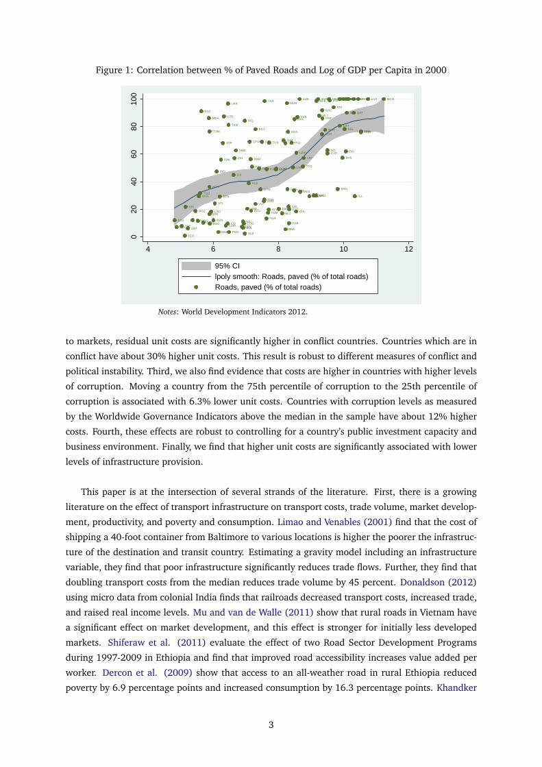
Figure 1: Correlation between % of Paved Roads and Log of GDP per Capita in 2000
ETH
BDISLE
TCD
ERI
LBR
MLI
MOZ
MDG
GHATGO
KGZ
AGO
MDA
SDN
COM
GIN
BGD
LSO
KEN
HTI
IND
MNG
SEN
PAK
STP
UZB
CMRCIV
UKR
TKM
PNG
DJI
IDN
SRB
GUY
NIC
BOLCOG
IRQ
SLB
HND
ALB
CPV
MAR
ECU
PRY
VUT
EGY
ROM
GTM
DZA
SURTON
THA
PER
FJI
FSMSLV
TUN
CUBDOM
ZAF
BLZ
JAMVCT
BRA
MUS
PAN
MYS
CRI
GAB
EST
POL
DMA
VEN
HRV
CHL
GRD
SVK
CZE
MEX
TTO
LBY
ARGOMNSAU
BRBSVN
MLT
KOR
GRC
PRT
BHR
NZLCYP
MACESP
PRI
BRN
ITA
KWT
ISR
BHS
FRA
BEL
FIN
SGPAUT
NLD
GBRIRLDNK
QAT
ISL
ARE
JPNNOR
LUX MCO
020
4060
8010
0
4 6 8 10 12
95% CIlpoly smooth: Roads, paved (% of total roads)Roads, paved (% of total roads)
Notes: World Development Indicators 2012.
to markets, residual unit costs are significantly higher in conflict countries. Countries which are in
conflict have about 30% higher unit costs. This result is robust to different measures of conflict and
political instability. Third, we also find evidence that costs are higher in countries with higher levels
of corruption. Moving a country from the 75th percentile of corruption to the 25th percentile of
corruption is associated with 6.3% lower unit costs. Countries with corruption levels as measured
by the Worldwide Governance Indicators above the median in the sample have about 12% higher
costs. Fourth, these effects are robust to controlling for a country’s public investment capacity and
business environment. Finally, we find that higher unit costs are significantly associated with lower
levels of infrastructure provision.
This paper is at the intersection of several strands of the literature. First, there is a growing
literature on the effect of transport infrastructure on transport costs, trade volume, market develop-
ment, productivity, and poverty and consumption. Limao and Venables (2001) find that the cost of
shipping a 40-foot container from Baltimore to various locations is higher the poorer the infrastruc-
ture of the destination and transit country. Estimating a gravity model including an infrastructure
variable, they find that poor infrastructure significantly reduces trade flows. Further, they find that
doubling transport costs from the median reduces trade volume by 45 percent. Donaldson (2012)
using micro data from colonial India finds that railroads decreased transport costs, increased trade,
and raised real income levels. Mu and van de Walle (2011) show that rural roads in Vietnam have
a significant effect on market development, and this effect is stronger for initially less developed
markets. Shiferaw et al. (2011) evaluate the effect of two Road Sector Development Programs
during 1997-2009 in Ethiopia and find that improved road accessibility increases value added per
worker. Dercon et al. (2009) show that access to an all-weather road in rural Ethiopia reduced
poverty by 6.9 percentage points and increased consumption by 16.3 percentage points. Khandker
3

et al. (2009) find that Bangladesh’s Rural Development Project and the Rural Roads and Markets
Improvement and Maintenance Project led to poverty reductions of 3-4% and 5-6%, respectively.
Jacoby and Minten (2009) find that an elimination of transport costs would substantially lower
poverty in their study region in Madagascar. Stifel et al. (2012) apply Jacoby and Minten’s method-
ology to a region in Ethiopia and arrive at a similar conclusion.
Second, while substantial progress is being made on evaluating the benefits of infrastructure,
research on the cost side is lagging behind. The paper relates to the recent effort in collecting data
on unit costs of different types of infrastructure investments across countries. It is is complementary
to the following studies: AFRICON (2008) analyze 115 road contracts in Sub-Saharan Africa and
find significant economies of scale for projects covering a length longer than 50 km. Given the rel-
atively small number of contracts, they have to aggregate various work activities into fairly coarse
groups to create comparisons. In addition to coverage of contracts of all regions worldwide, the
advantage of our paper is that we can control for systematic differences in the cost of construction
by including fixed effects at the very detailed work activity level. Two studies by Alexeeva et al.
(2008) and Alexeeva et al. (2011) examine evidence for corruption in the roads sector, using data
on 109 road work contracts and 76 supervision consultancy contracts in 13 Sub-Saharan African
countries, and a sample of 200 completed and ongoing road contracts in 14 European and Central
Asian countries, respectively. This paper differs from these two studies in that we focus on differ-
ences across countries, rather than the link between the bidding process, input costs and the unit
cost of particular road work contracts1. Buys et al. (2010) use a subset of 465 roads contracts
in Sub-Saharan African countries from the ROCKS database to argue that upgrading of the roads
network could lead to an expansion of trade by US$250 billion over 15 years, at a cost of US$20
billion for upgrading and US$1 billion annually for maintenance costs.
Third, the paper relates to a fairly recent literature on government procurement processes and
waste associated with it. Bandiera et al. (2009) test for active (for example, corruption) and passive
waste (for example, the inability of the civil servant to select the cheapest product) in the procure-
ment of 21 generic goods by Italian public bodies and find substantial heterogeneity in prices paid
by different types of bodies, with the average ministry paying about 40% higher prices compared to
semi-autonomous bodies; passive waste is found to account for about 83% of waste. Di Tella and
Schargrodsky (2003) find that a crack-down on corruption led to a 10-15% decline in prices paid by
hospitals in Buenos Aires for basic supplies compared to the pre-crack-down period. Several studies
investigate the bidding behavior of firms and efficiency of auctions in public procurement. Hyyti-
nen et al. (2007) study the procurement of cleaning contracts in municipalities in Sweden and find
that in 58% of the time, the lowest bidder does not win the auction and then contrast the behav-
iors of left-wing and right-wing governments. Huysentruyt (2011) examines 457 completed DFID
contracts and compares for-profit and non-profit firms’ bidding and contract implementation char-
acteristics. She finds that contract renegotiations take place in 60% of all contracts, with the cost of
renegotiations being about 30-50% higher when contracting with for-profit organization compared
1Ideally we would have liked to test their hypotheses on the larger data set we employ in our study; unfortunately,detailed bidding information was only collected for a small number of contracts in the database.
4

to non-profit organizations. Increasing attention has also been attributed to infrastructure auctions
in developing countries. Estache and Iimi (2009) find joint bidding to be pro-competitive, especially
when involving local entreprises from analysing 86 road work contracts. Estache and Iimi (2010)
use data from 45 auctions in the roads sector of projects by the World Bank and the former Japan
Bank for International Cooperation and find that in the roads sector bids submitted by entrant bid-
ders are substantially more aggressive.
Finally, we aim to contribute to the literature on conflict and corruption. To our knowledge, the
only study quantitatively investigating the link between conflict and the cost of transport infrastruc-
ture is Benamghar and Iimi (2011) who use data on 157 rural road projects in Nepal and show that
the number of security incidents is significantly and and positively correlated with the value of sub-
mitted bids, cost overruns, and project delays. Considering corruption in transport infrastructure,
Olken (2007) finds that missing expenditures amounted to on average 24% of the total cost of the
road in his experiment in Indonesia. See Blattman and Miguel (2010) for a recent review on the
literature on conflict and Olken and Pande (2012), Zitzewitz (2012) and Banerjee et al. (2012) on
corruption in developing countries.
The paper is organized as follows. Section 2 sets the scene for our focus on conflict and cor-
ruption. Section 3 presents a theoretical framework for analyzing the drivers of unit costs of road
construction and maintenance. Section 4 describes our data. Section 5 outlines the econometric
specification; section 6 discusses the results and sketches avenues for further research; the final
section concludes.
2 Conflict and Corruption in the Roads Sector
The focus of our analysis is on the link between conflict and corruption and unit costs of road work
activities. The focus on conflict is motivated by the fact that 1.5 billion people live in conflict-
affected or fragile states, and these states lag behind on measures like poverty reduction and other
developmental outcomes (World Bank 2011b). If these finance constrained states face high road
construction costs, and roads construction and a better network reduce conflict by raising the op-
portunity cost of joining rebel groups through employment, as well as improved economic outcomes
through better connectivity, then they might be trapped in an equilibrium with high costs of trans-
port infrastructure and instability. Further, public work contracts, including roads, are subject to
substantial levels of corruption. According to Transparency International’s Bribe Payers Survey of
over 3,000 business executives worldwide, public works contracts and construction is the sector
with the highest propensity of paying bribes to officials and other firms (Transparency International
2011). As this paper attempts to establish a first set of facts on differences in costs, a focus on the
link between corruption and costs is a natural priority.
A review by the World Bank’s Transport Research Support Program on the roads sector in con-
flict countries states that “...projects that take place in conflict settings would almost always be more
costly than in other settings because of challenges such as insecurity and low government capacity”
5

(Rebosio and Wam 2011). Higher costs can be due to the costs of monitoring of the security sit-
uation of an area, potentially undergoing substantial risks to visit the construction site, and the
associated limited planning possible. In addition to protection of the staff working on the particular
roads project, firms also risk that supplies are cut off due to disruptions of transport networks. If
conflict takes place along ethnic lines, road construction firms might need to ensure to employ an
ethnically balanced workforce, in order not to further fuel the conflict or becoming targets of vio-
lence themselves. Consultations with communities, while helpful, are also significantly adding to
the cost of construction. Not only the construction but also the procurement process can be riskier
in conflict countries. Rebosio and Wam (2011) and Benamghar and Iimi (2011) give evidence for
these effects on risks and costs from Nepal: a government employed road engineer was killed in
the Terai regions; road construction teams were constantly monitoring the security situation and
adjusting their operations accordingly; in certain regions violence and intimidation were employed
during the bidding process to prevent firms from submitting a bid for profitable project.
Allegations of fraud, corruption or collusion were made in about one fourth of the 500 approved
World Bank financed projects with a road component between 2000-2010 (World Bank 2011a).
Roads contracts procured through the World Bank are usually awarded in a one stage sealed bid
auction, with the lowest bidder winning the auction. Alexeeva et al. (2011) find that in about 20%
of the auctions in their sample of 200 contracts in Europe and Central Asia, at least 50% of firms who
acquired bidding documents do not bid, the winning bid is not selected for detailed examination,
or there is a time overrun of more than 30% of the contracted period. The estimates of costs of
collusion and cartels in the road sector are large and range between 8% and 60% (World Bank
2011a). Considering that substantial resources are allocated to road construction and maintenance
(US$56 billion between 2000-2010 by the World Bank alone), this represents a massive waste
of funds. Further evidence from investigations discussed in (World Bank 2011a) is striking: in
Bangladesh, companies paid officials up to 15% of the contract value in exchange for award of the
contract. In an African country, fraudulent claims such as cement contents and thinner layers than
specified accounted for 15-20% of the bid price; the use of substandard materials imposes costs
ex-post through higher maintenance costs and costs on vehicle drivers due to worse road conditions
and might eventually lead to even negative rates of return of a particular project (Kenny 2009).
3 Theoretical Framework
This section develops a simple theoretical framework with the purpose of guiding the empirical
analysis. Consider a particular type of road work activity, for example, a construction of a new 2
lane highway. Denote the length of the highway as q. Firms employ labor x1 and capital x2 in the
production of highways and minimize a cost function
minx1,x2
w1 x1+w2 x2 subject to q = f (x1, x2) (1)
where w1 is the price of labor and w2 is the price of capital. Firms are assumed to be price takers
in input markets. Further, assume that the firm has a Cobb-Douglas production function so that
6
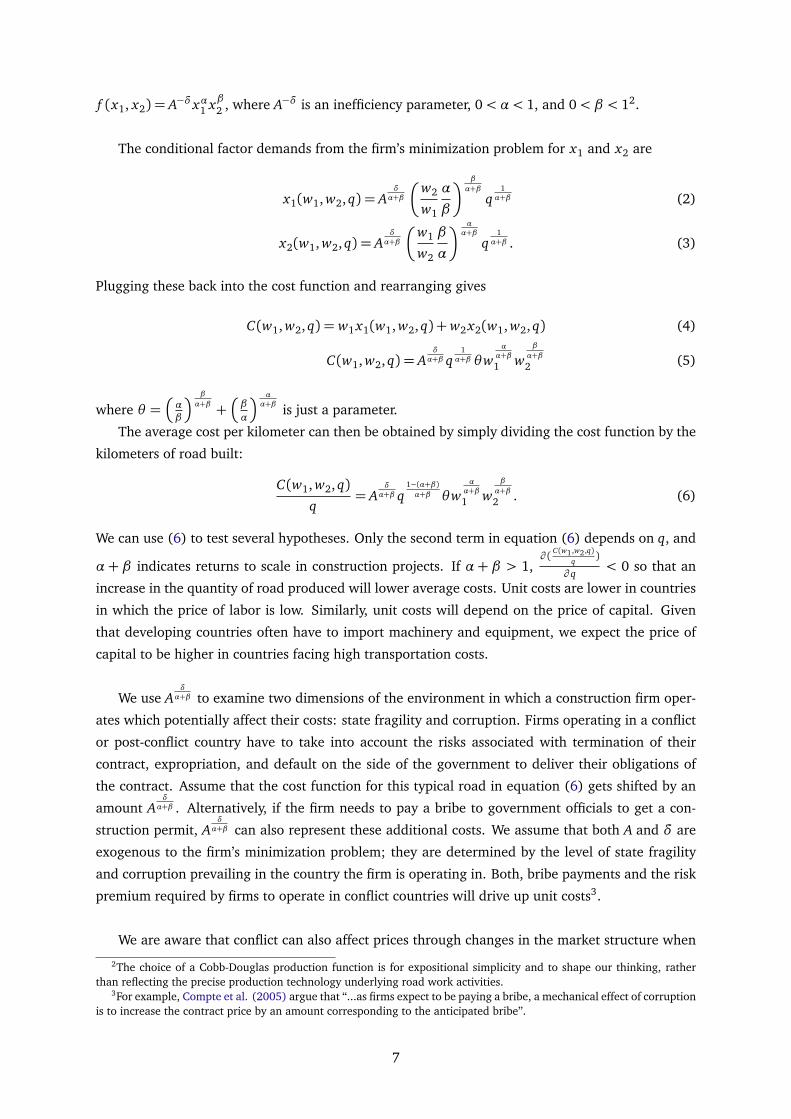
f (x1, x2) = A−δxα1 xβ2 , where A−δ is an inefficiency parameter, 0< α < 1, and 0< β < 12.
The conditional factor demands from the firm’s minimization problem for x1 and x2 are
x1(w1, w2, q) = Aδα+β
�
w2
w1
α
β
�
β
α+β
q1α+β (2)
x2(w1, w2, q) = Aδα+β
�
w1
w2
β
α
�αα+β
q1α+β . (3)
Plugging these back into the cost function and rearranging gives
C(w1, w2, q) = w1 x1(w1, w2, q) +w2 x2(w1, w2, q) (4)
C(w1, w2, q) = Aδα+β q
1α+β θw
αα+β1 w
β
α+β2 (5)
where θ =�
αβ
�
β
α+β +�
β
α
�αα+β is just a parameter.
The average cost per kilometer can then be obtained by simply dividing the cost function by the
kilometers of road built:
C(w1, w2, q)q
= Aδα+β q
1−(α+β)α+β θw
αα+β1 w
β
α+β2 . (6)
We can use (6) to test several hypotheses. Only the second term in equation (6) depends on q, and
α+ β indicates returns to scale in construction projects. If α+ β > 1,∂ ( C(w1,w2,q)
q )
∂ q< 0 so that an
increase in the quantity of road produced will lower average costs. Unit costs are lower in countries
in which the price of labor is low. Similarly, unit costs will depend on the price of capital. Given
that developing countries often have to import machinery and equipment, we expect the price of
capital to be higher in countries facing high transportation costs.
We use Aδα+β to examine two dimensions of the environment in which a construction firm oper-
ates which potentially affect their costs: state fragility and corruption. Firms operating in a conflict
or post-conflict country have to take into account the risks associated with termination of their
contract, expropriation, and default on the side of the government to deliver their obligations of
the contract. Assume that the cost function for this typical road in equation (6) gets shifted by an
amount Aδα+β . Alternatively, if the firm needs to pay a bribe to government officials to get a con-
struction permit, Aδα+β can also represent these additional costs. We assume that both A and δ are
exogenous to the firm’s minimization problem; they are determined by the level of state fragility
and corruption prevailing in the country the firm is operating in. Both, bribe payments and the risk
premium required by firms to operate in conflict countries will drive up unit costs3.
We are aware that conflict can also affect prices through changes in the market structure when
2The choice of a Cobb-Douglas production function is for expositional simplicity and to shape our thinking, ratherthan reflecting the precise production technology underlying road work activities.
3For example, Compte et al. (2005) argue that “...as firms expect to be paying a bribe, a mechanical effect of corruptionis to increase the contract price by an amount corresponding to the anticipated bribe”.
7

firms are driven out of business, or through a price boom following the end of a conflict as demand
for reconstruction increases. Further, corruption in the roads sector can be at three levels, with
varying effects on efficiency. First, it can take at the level of the government when government
officials receive side-payments to either select a contract from a particular firm, or to process docu-
ments of the operating firm. This results in higher unit costs and allocative inefficiency if contracts
are not awarded to the most competitive firm. Second, individuals working for companies in the
construction sector might inflate costs and use part of of these resources to extract side payments
for themselves. The higher unit cost in turn decreases the likelihood of the project to be selected
ex-ante by lowering the net present value or rate of return. Third, companies might not respect the
contracted standards by using fewer or inferior materials. Here we only focus on the first level. We
discuss further hypotheses how conflict and corruption affect roads construction costs in the final
section as avenues for future research.
It is also worth highlighting several issues relevant to the procurement of roads which we do
not consider in our simple model4. First, the market structure of the road construction sector and
tender procedures affect how many firms will submit bids for a project, thereby determining ex-ante
competition and the value of bids (Li and Zheng 2009). Second, if firms collude in the tendering
phase, they can affect the price of the road contract (Pesendorfer 2000). Third, once a government
has signed a contract with a firm for a road construction project, the firm can extract rents from
the government, a problem referred to as hold-up in the literature (Board 2011). In the absence of
data on the market structure, values of submitted bids for work activities as well as the difference in
costs between contracted and actual costs for each work activity, we are not able to uncover these
effects. The main rationale for the simple cost minimization framework is to inform our way of
thinking about the deeper determinants of costs and input prices in an economy and to serve as
a guide for the estimation. We return to market structure, collusion and hold up problems when
discussing avenues for further research.
4 Data
We use unit cost data from the Roads Cost Knowledge System (ROCKS), Version 2.3, developed by
the World Bank’s Transport Unit. Motivated by the lack of comparable information on costs of road
work activities across countries, the database was started in 2001 with the aim of developing “an
international knowledge system on road work costs - to be used primarily in developing countries
- to establish an institutional memory, and obtain average and range unit costs based on historical
data that could ultimately improve the reliability of new cost estimates and reduce the risks gen-
erated by cost overruns” (World Bank 2006). The focus of this section is on describing the data;
we discuss issues due to selection in detail in the next section. The data stems from World Bank
financed projects and is collected in collaboration with road agencies in the respective countries us-
ing information from Implementation Completion Reports, Pavement Management Systems Review
Reports, Works Contracts, Appraisal Reports and Highway Development and Management Studies.
4See Moavenzadeh (1978) for a discussion how the construction sector is generally differs from other sectors.
8

The data collection exercise was first conducted in five pilot countries, Bangladesh, India, Thai-
land, Viet Nam, Philippines; in 2002 a second set of countries was added including Ghana, Uganda,
Poland, Armenia; in 2004, Lao, Kyrgyz, Kazakhstan, Ethiopia, Nigeria, and Serbia and Montenegro
were added. As Table 1 shows, the current version of the database contains data from 3,322 work
activities in 99 low and middle income countries out of which 23% are located in low income coun-
tries5. Contracts date between 1984 and 2008, with 82% of contracts taking place between 1996
and 2006. Tables 17 and 18 in the appendix show the distribution of projects by country over time.
Table 1: Complete ROCKS Database for Low and Middle Income Countries
N Percent
Low income 780 23.48Lower middle income 1,352 40.70Upper middle income 1,190 35.82Total 3,322 100
Notes: income classification based on World Devel-opment Indicators 2012.
The ROCKS database is based on 5 concepts (World Bank 2006). First, to allow for comparabil-
ity of similar activities, road works are classified into categories: road development works and road
preservation works. Within these two categories, projects are further divided into work class, work
type and work activity. The detailed list of these sub-categories is presented in Tables 12 and 13 in
the appendix. Second, comparisons are made possible through unit costs which are defined either
as costs per square meter or costs per km. Third, the ROCKS database defines a minimum data
requirement which is required to make the data comparable (e.g. country, date, project or source
name, currency, unit cost, work type, cost type). Fourth, to add flexibility, road agencies are able
to enter highly recommended data (e.g. predominant work activity, total cost, length and duration,
carriage width, terrain type) and optional data (e.g. number of bidders, value of individual bids,
unit costs of asphalt concrete, Portland cement concrete). Unit costs include civil works costs such
as mobilization, pavement drainage, major structures and line markings; they exclude agency costs
such as design, land acquisition, resettlement and supervision. Fifth, these costs are deflated to
the year 2000 using the domestic consumer price index, and then converted into US$ using the
exchange rate in 2000. Bringing unit costs back to the same reference year and the same currency
is crucial to allow for comparison across projects.
Unit costs are provided for programs or sections; a program is a part of a loan or credit, or a
number of road sections combined. Sections define unit costs for road works on particular segments
of a road. In either case, we have information on the name of the project the program or section
is part of. Considering that a range of reports is used for the data collection, 44% of entries are
5We exclude duplicates of 31 contracts for which we have the same entry for country, date, cost per km, cost type,work activity, length, width, shoulder and lanes. We also drop two contracts for Reconstruction Bituminous (one inIndia and one in Bangladesh) for which the recorded costs were US$218 and US$2,289; the median cost of the 595Reconstruction Bituminous work activities of our database is US$195,516 per km so these two entries are likely to beincorrect.
9

estimated costs, 27% are contracted costs, and 29% are actual costs. For some projects the database
contains costs on all of the three categories. We include all of the available cost data. Unit costs
from these different sources often differ by a large extent, so knowledge of the source is critical
to compare unit costs. Individual road works activities also sometimes form part of a larger roads
project. In order to account for the fact that there might be various costs types for the same projects,
as well as various different work activities for the same project, we cluster the standard errors by
country to allow for arbitrary correlation of costs within the same country.
Tables 14 to 16 in the appendix show the mean, median, maximum and minimum cost of various
work types and work activities for both preservation and development works. The most expensive
development work type is a new six lane expressway followed by a four lane expressway, while
for preservation works the most expensive work type is concrete pavement restoration followed by
strengthening. Zooming one level further in we see that the most expensive development activity
has been further classified as a new bituminous six lane expressway, and the most expensive preser-
vation work activity is a concrete slab replacement followed by reconstruction in bituminous and
concrete.
Table 2 shows the range of average unit costs for a precisely defined work activity: asphalt over-
lays between 40 to 59 mm between 1996-1998 and 2006-2008 ranked by the cost in US$ per km.
We limit the time window in order not to conflate differences in unit costs with changes in input
prices which might affect economies differently. What is striking is that even for a narrowly defined
time window and work activity, there are differences in unit costs of a factor between three to four.
Using these unit costs, an asphalt overlay for a length of 100 km would cost US$3,300,000 in the
Dominican Republic in 1997, compared to US$11,000,000 in Tanzania in 1996, or US$10,500,000
in Pakistan in 1998. Two sources of heterogeneity remain. While costs per square kilometer of a
precisely defined work activity in a short time window are likely to be comparable, one could argue
that different road widths might contribute to higher unit costs. Table 19 in the appendix shows that
the ranking is largely unaffected when using unit costs per square meter in 1996-19986. Second,
we pool across different sources of costs here, so the costs could be estimated, contracted or actual
costs. However, the difference in unit costs of a factor of three to four is unlikely to be due to just
differences in the source of costs7. We do not have enough observations for narrow work activities
within these different cost types to separately show the differences for a large set of countries. To
account for systematic differences across cost types, we have also compared the cost of construction
projects, after partialling out the effects of cost types in a regression. The order of countries as well
as range of unit costs remains substantively the same.
The database also contains bidding information for a subset of 266 work activities across 35
countries and the 5 regions. The minimum number of bidders is 1 and the maximum number is
6Costs per square meter are missing for many observations in 2006-2008, so we only show unit costs of work activitiesfrom the earlier period.
7Flyvbjerg et al. (2003) finds average cost overruns for roads are about 20% for projects in Europe and North America;Alexeeva et al. (2008) find average cost overruns by country for the DRC, Malawi, Tanzania, Mozambique, Ghana andNigera to be between 12.05% and 39.72%; Alexeeva et al. (2011) find average cost overruns by country for Georgia,Serbia, Estonia, Armenia, Macedonia, Albania, Azerbaijan and Kazakhstan to be between 6% and 47%.
10
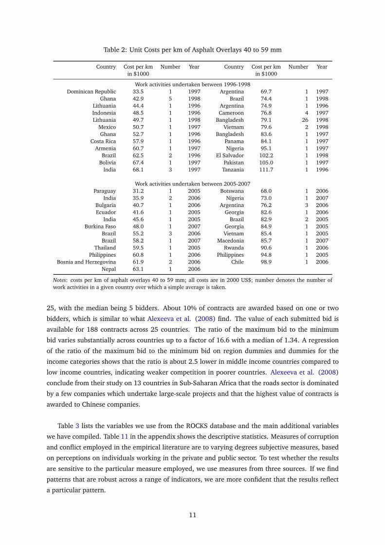
Table 2: Unit Costs per km of Asphalt Overlays 40 to 59 mm
Country Cost per km Number Year Country Cost per km Number Yearin $1000 in $1000
Work activities undertaken between 1996-1998Dominican Republic 33.5 1 1997 Argentina 69.7 1 1997
Ghana 42.9 5 1998 Brazil 74.4 1 1998Lithuania 44.4 1 1996 Argentina 74.9 1 1996Indonesia 48.5 1 1996 Cameroon 76.8 4 1997Lithuania 49.7 1 1998 Bangladesh 79.1 26 1998
Mexico 50.7 1 1997 Vietnam 79.6 2 1998Ghana 52.7 1 1996 Bangladesh 83.6 1 1997
Costa Rica 57.9 1 1996 Panama 84.1 1 1997Armenia 60.7 1 1997 Nigeria 95.1 1 1997
Brazil 62.5 2 1996 El Salvador 102.2 1 1998Bolivia 67.4 1 1997 Pakistan 105.0 1 1997
India 68.1 3 1997 Tanzania 111.7 1 1996
Work activities undertaken between 2005-2007Paraguay 31.2 1 2005 Botswana 68.0 1 2006
India 35.9 2 2006 Nigeria 73.0 1 2007Bulgaria 40.7 1 2006 Argentina 76.2 3 2006Ecuador 41.6 1 2005 Georgia 82.6 1 2006
India 45.6 1 2005 Brazil 82.9 2 2005Burkina Faso 48.0 1 2007 Georgia 84.9 1 2005
Brazil 55.2 3 2006 Vietnam 85.4 1 2005Brazil 58.2 1 2007 Macedonia 85.7 1 2007
Thailand 59.5 1 2005 Rwanda 90.6 1 2006Philippines 60.8 1 2006 Philippines 94.8 1 2005
Bosnia and Herzegovina 61.9 2 2006 Chile 98.9 1 2006Nepal 63.1 1 2006
Notes: costs per km of asphalt overlays 40 to 59 mm; all costs are in 2000 US$; number denotes the number ofwork activities in a given country over which a simple average is taken.
25, with the median being 5 bidders. About 10% of contracts are awarded based on one or two
bidders, which is similar to what Alexeeva et al. (2008) find. The value of each submitted bid is
available for 188 contracts across 25 countries. The ratio of the maximum bid to the minimum
bid varies substantially across countries up to a factor of 16.6 with a median of 1.34. A regression
of the ratio of the maximum bid to the minimum bid on region dummies and dummies for the
income categories shows that the ratio is about 2.5 lower in middle income countries compared to
low income countries, indicating weaker competition in poorer countries. Alexeeva et al. (2008)
conclude from their study on 13 countries in Sub-Saharan Africa that the roads sector is dominated
by a few companies which undertake large-scale projects and that the highest value of contracts is
awarded to Chinese companies.
Table 3 lists the variables we use from the ROCKS database and the main additional variables
we have compiled. Table 11 in the appendix shows the descriptive statistics. Measures of corruption
and conflict employed in the empirical literature are to varying degrees subjective measures, based
on perceptions on individuals working in the private and public sector. To test whether the results
are sensitive to the particular measure employed, we use measures from three sources. If we find
patterns that are robust across a range of indicators, we are more confident that the results reflect
a particular pattern.
11

Table 3: Description of Main Data and Sources
Variable Description Source
Log of Cost Log of unit cost of a particular road work activ-ity (1984-2008)
ROCKS dataset, World Bank
Estimate =1 if estimated costs ROCKS dataset, World BankContract =1 if contracted costs ROCKS dataset, World BankActual =1 if actual costs ROCKS dataset, World BankFlat =1 if terrain is flat ROCKS dataset, World BankHilly =1 if terrain is hilly ROCKS dataset, World BankMountainous =1 if terrain is mountainous ROCKS dataset, World BankRolling =1 if terrain is rolling ROCKS dataset, World BankLog of Ruggedness Log of Terrain Ruggedness Index, representing
the average ruggedness of a country measuredas hundred of meters of elevation difference forgrid points 926 meters apart
Nunn and Puga (2012)
Log of Distance tothe nearest ice freecoast
Log of average distance to nearest ice-free coast(1000 km)
Nunn and Puga (2012)
Log of Rainfall Log of yearly precipitation in 100s mm Dell et al. (2012)Population Density Population Density (100 people per square km),
1960-2012World Development Indicators
Log of Surface Area Log of Surface Area (1,000 square kilometers) World Development IndicatorsLog of GDP Log of GDP per capita (1984-2008), constant
2000 US$World Development Indicators
ACD Conflict =1 if country is in a conflict Armed Conflict DatasetWGI Instability Index of political instability and violence from
World governance Indicators (1996-2012), re-defined to: -1.26 (lowest) to 2.21 (highest)
World Governance Indicators
TI Corruption Corruption index from Transparency Interna-tional, survey 2008, rescaled to 0.1 (lowest cor-ruption), 5.6 (highest corruption)
Transparency International
WGI Corruption Index of corruption from World Governance In-dicators (1996-2012), redefined to: -1.45 (low-est corruption) to 1.6 (highest corruption)
World Governance Indicators
PIMI Public Investment Management Index, 2011,measured on scale from 0 (worst) to 4 (best)
Dabla-Norris et al. (2011)
Log of DB Contract Number of days it takes to enforce a contract,from Doing Business Indicators 2007
Doing Business Indicators
First, our most direct measure for conflict episodes comes from the version 4-2012 of the
UCDP/PRIO Armed Conflict Dataset, published by the Uppsala Conflict Data Program (UCDP) and
the International Peace Research Institute, Oslo (PRIO)8. Readers are referred to Gleditsch et al.
(2002), Themnér and Wallensteen (2012) and the Dataset Codebook for details. UCPD defines
conflict as “a contested incompatibility that concerns government and/or territory where the use
of armed force between two parties, of which at least one is the government of a state, results in
at least 25 battle-related deaths” We follow Miguel et al. (2004) and focus on internal armed con-
flicts between the government and an internal party with and without outside intervention which
accounts for 88.5% of the conflicts recorded in the database. We define a project as being carried
8The other potential conflict data set is the Correlates of War data set. Due to concerns over transparency andconsistency as well as a high threshold of deaths (Miguel et al. 2004) we prefer the Armed Conflict Dataset (ACD).
12

out in a conflict state if the state is in conflict in the year the road work activity is recorded; a
country is likely not to return to full stability after the end of a conflict, so we also create a variable
that defines the country as being in a post conflict period for 5 years after the end of a conflict, or
until the country reverted back into conflict. There are 187 conflict and post-conflict periods in the
countries covered in our data.
Second, we use data from the Worldwide Governance Indicators (WGI) which are based on data
from household and firm surveys, commercial business information providers, non-governmental
organizations and public sector organizations. Six indicators capture different aspects of gover-
nance in 200 countries since 1996. We use the variables on ’control of corruption’ and ’political
stability and absence of violence/terrorism’. The control of corruption variable measures “percep-
tions of the extent to which public power is exercised for private gain, including both petty and
grand forms of corruption, as well as ’capture’ of the state by elites and private interests” and the
variable political stability and absence of violence/terrorism reflects “perceptions of the likelihood
that the government will be destabilized or overthrown by unconstitutional or violent means, in-
cluding politically-motivated violence and terrorism” (Kaufmann et al. 2010). These indicators are
measured between -2.5 and 2.5 where higher numbers reflect lower levels of corruption and politi-
cal instability. We multiply the variables by (-1) and rename the variables ’Corruption’ and ’Political
Instability’ so that higher numbers reflect higher levels of corruption and political instability.
Third, we use Transparency International’s 2008 Corruption Perception Index which allocates
scores to countries from 1 to 10, where 0 equals the highest level of perceived corruption and 10
equals the lowest level of perceived corruption. We rescale the variable so that 10 is the high-
est level of corruption. Graf Lambsdorff (2005) and Thompson and Shah (2005) underscore that
the Corruption Perception Index is inappropriate for comparison of countries across time, due to
changes in methodology as well as data sources underlying the index. We use 2008 because this is
the earliest year with the highest number of countries covered. We have also assembled the index
for the years 1998-2011 and our results are robust to using the indicator from earlier years (1998-
2007) and later years (2009-2012)9.
9A popular source, due to its coverage across countries and time, for perception based data on institutions is theInternational Crisis Research Group (for example, Alesina and Weder (2002), Fisman and Miguel (2007), Ahmed (2012),Svensson (2005), Wei (2000)). The International Crisis Research Group compiles yearly data on 22 indicators measuringpolitical, financial and economic risk between 1984 and 2012. Corruption is measured from 0 (high corruption) to 6 (lowcorruption) as a component of political risk. We do not include this measure for several reasons. First, Treisman (2007)has highlighted various questionable scores in the corruption indicator, both in the cross-section of countries as well asjumps in the indicator over time which do not seem correspond to specific country level policies. We highlight someadditional peculiarities here. For example, in 2000, Austria had the same level of corruption (a score of 4/6) as Congo,Iran, Libya and the United States. In the same year, Transparency International gives Austria a score of 7.7/10 where10 is the least corrupt, Congo has it’s earliest ranking in 2004 with 2.3/10, Iran gets 3.3/10, Libya has 2.1/10 in 2003,and the United States receives 7.8/10. There are also large discrepancies with the Worldwide Governance Indicators. Wedivide the set of countries into deciles for the year 2000 where higher deciles correspond to less corruption, and showthat the difference in the location of countries is up to 8 deciles. For instance, Ireland ranks in the 10th decile in theWGI score, while it falls into the second decile according to the ICRG’s ranking. Contrarily, the Congo falls within theeight percentile in fighting corruption according to the ICRG measure, while it falls into the second lowest percentileof corruption according to the WGI measure. For some countries there are large jumps. For example, in 1989 Niger’scorruption measure was with 4 on par with Italy’s, dropped to 3 in 1991 and then to 0 in 1997. Kenya’s ICRG scoredropped from 3.46 in 2003 to 0.5 in 2006. Lebanon’s score dropped from 4 in 1995 to 1.75 in 1996. The averageof the cross sectional correlation across the full set of countries between 1996-2011 is 0.86, for our sample of low and
13

The correlation between the WGI political instability indicator and the ACD conflict dummy is
0.58, and the correlation between the Transparency International measure and the WGI corruption
measure is 0.81. Both correlations are significant at the 1 percent level. For the empirical analysis
we create lagged three year averages of the two WGI measures. The data for our other explanatory
variables are described in section 8.1 in the appendix.
5 Estimation and Identification
To obtain an estimable equation, we take logs of equation (6) and get
lnC(w1, w2, q)
q=
δ
α+ βA+ lnθ +
1− (α+ β)α+ β
ln q+α
α+ βln w1+
β
α+ βln w2. (7)
Rewriting average costs C(w1,w2,q)q
as c, denoting δα+β = γ, 1−(α+β)
α+β = φ1, αα+β = φ2, β
α+β = φ3,
adding an error term and fixed effects for work activities, time and region as well as subscripts for
work activities, work types, countries and time, we obtain
ln capit =γAi t + lnθ +φ1 ln qapit +φ2 ln w1apit +φ3 ln w2apit
+κapit +ωa +τt + ξpt +ρap + εapit (8)
for work activity a = 1, . . . , A, work type p = 1, . . . , P, country i = 1, . . . , N , and time t = 1, . . . , T ,
where c is the cost per kilometer, q is a dummy variable that is equal to one if the length of the road
is above 50 km; we do not have data on the cost of labor and capital for each construction project.
Rather than estimating the technological parameters, our controls are selected to control for the
deep determinants of factor prices. The cost of capital is going to be a function of transport costs,
so we include the distance to the nearest ice-free coast from Nunn and Puga (2012) as a measure of
the price of capital and equipment. For about half of the road work activities we know whether the
terrain on which the road works are undertaken is flat, mountainous, hilly or rolling. We include
these as dummy variables, and additionally include a measure of country-level ruggedness to ac-
count for higher input costs required on more rugged terrain. Given that unit costs might be higher
in countries with high levels of rainfall, we include the three year average of lagged precipitation.
We further include the log of GDP per capita to proxy for the price of labor and capital. We then use
our measures of corruption and conflict to proxy for A, and include two dummy variables indicating
that a country is above the median level of conflict or corruption of the sample10. Due to high levels
middle income countries the average cross sectional correlation is 0.59, ranging from 0.37 in 1998 to 0.70 in 2011. Yearlychanges are uncorrelated for 4 periods, with an average correlation of 0.2 for the remaining periods in the full sample andsimilar patterns in the our sample of countries. Wei (2000) uses an average of the ICRG measure between 1991-1993, andSvensson (2005) uses either an average between 1982-2001 or the year 2001 in a cross section of countries. Given thatcross-sectional variation is rather high, in these settings different measures produce similar results. Using these measuresin a panel setting has been seriously questioned (Treisman 2007; Graf Lambsdorff 2005). Alesina and Weder (2002)use five-year averages for their main results, but emphasize that results in first differences should be interpreted ’verycautiously’. Ahmed (2012) does not show the robustness of his results when using alternative measures of corruptionin his regressions using country fixed effects. Finally, Graf Lambsdorff (2005) notices that the ICRG Corruption variablereflects the political risk associated with corruption, rather than a country’s level of corruption; the ICRG website does notprovide information on how the scores are constructed. We therefore rely on the WGI and the TI corruption measures.
10We take the median of distinct country-year observations we have in the sample.
14

of correlation between these measures, we enter them in separate regressions. Appreciating that
road work contracts require a substantial amount of time to negotiate, we lag time varying country
level controls by one period.
To account for differences in the source of unit costs and procurement, κapit is a vector of
dummy variables capturing whether the source of costs is estimated or contracted costs with the
base category being actual costs. All models include work activity fixed effects ω to control for
systematic differences in costs across work activities, year fixed effects τ to account for worldwide
construction industry trends, interaction terms between work type and 5-year dummies ξ to allow
for differences in the evolution of costs for different work types, region fixed effects ρ, and an error
term ε11. We have missing values for certain countries for some of the explanatory variables. In this
case, we follow a procedure known as modified zero-order regression outlined by (Greene 2003,
p.60) in which we include a dummy variable that is equal to one if the variable is missing, and
replace the missing observations with zero. We are not interested in the coefficients of the missing
dummy variables, so do not report them when discussing the results.
In order to interpret the coefficient estimates on the included variables as causal relationships,
we would require that E(Xapct |εapit = 0) where Xapit denotes a vector of all included controls. This
is an implausible assumption. While it is unlikely that there is reverse causality from unit costs
to the control variables, omitted variables might still bias our parameter estimates. Unfortunately,
many of the controls are time invariant, and we do not have enough variation over time to include
country fixed effects to account for time invariant unobservable characteristics and still identify
the coefficient estimates of time-varying variables. The parameters estimates should therefore be
interpreted as statistical associations, which still contain valuable insights. As a robustness check
we will also estimate equation (8) with country fixed effects to test whether the road work activity
characteristics, which have substantial within country variation, remain significant.
5.1 Selection
Our unit cost sample is selected along three dimensions. First, we only observe road work activities
for which the World Bank provided a loan12. Given that this is the only available large database,
our findings need to be interpreted in the context of this subset of work activities conducted in
collaboration with the World Bank.
Second, from inspection of tables 17 and 18 in the appendix it becomes clear that the distribu-
tion of road work activities is not a random sample of contracts per country for each year. Rather,
11Table 20 in the appendix shows the coefficients of the work type dummy variables including and excluding countrylevel controls. In the discussion of the results in the next section, we always control for work activity fixed effects, but donot discuss the differences in unit costs across these categories as this is not the main focus of this paper.
12It is not clear in which direction this would bias our estimates. If the World Bank, through its procurement guidelines,is able to impose stricter procedures in more corrupt countries than the government, we would underestimate the effectof corruption. Without the stringent guidelines, the government would have to pay a higher premium in high corruptioncountries. On the other hand, governments in corrupt countries are potentially better able to limit the magnitude of sidepayments necessary to carry out a work activity; this would indicate that our estimates of the effect of corruption arehigher than the cost faced by governments.
15
as mentioned in section 4, the data are clustered around pilot countries, with additional countries
being added gradually. We have been told from the responsible for the database that selection into
the database out of the population of projects carried out by the World Bank does not follow any
specific pattern, so that we regard it as random. To capture time invariant unobservables determin-
ing selection as a pilot country, we also include a dummy variable that is equal to one if a country
belongs to the first two sets of pilot countries13.
Third, we only observe costs for projects that were implemented, so out of the population of
potential road work activities we miss projects which have not been started14. Considering that the
net present value of a project at time=0 is N PV0 =−I0+(B1− C1)/(1+ r)1+ . . .+(BT − CT )/(1+
r)T , projects which appear in the database must have low enough costs (initial costs I0 as well as
maintenance costs C) or high enough benefits B. We therefore observe a truncation of the response
variable (those with high project costs and low benefits). We can examine the bias introduced by
such truncation. Assume that the true model is c = β0 + β1 x + u where c are unit costs, β0 is a
constant, β1 is our coefficient of interest, and u is an error term. Consider a project with the same
level of benefits in two countries. Let x be corruption, assume that corruption increases costs so
that β1 > 0, and that one country has a high level of corruption, while the other country has a low
level of corruption. While the project is undertaken in the low corruption country, it might fail to
generate a high enough NPV in the high corruption country. We therefore miss projects with high x
and high u. Thus, thus x and u will be negatively correlated in the truncated sample and the OLS
estimate of β1 will be downward biased (towards zero), underestimating the effect of corruption
on unit costs. Similarly, assume that x is a measure of flatness of the terrain, so that higher values
correspond to flatter terrain, and lower values to mountainous terrain. Since it is cheaper to build
a road on flat terrain, β1 < 0. Consider again a project yielding the same level of benefits in a flat
and in a mountainous country. Following the logic above, a project yielding the same benefits is
more likely to be in our sample in flat terrain (high x) and we will tend to miss out on projects in
mountainous areas, so that x and u will be positively correlated in the truncated sample and the
OLS estimate of β1 will be upward biased, i.e. again towards zero. In this case, we will under-
estimate the cost-reducing effect of flat terrain. This suggests that we will tend to underestimate
effects in general so that our estimates can be viewed as conservative. If the benefits of a project
are a function of the individuals affected by the improved road, and congestion costs are important,
we would expect the benefit of transport infrastructure to be higher in densely populated areas, so
that projects are more likely to be selected even if costs are higher than in an otherwise equivalent
context. Unfortunately, we do not have information on projects which have not been carried out. We
are therefore limited to controlling for population density to account for selection on observables.
6 Empirical Results and Discussion
We start by presenting the main results from equation (8) including our measures of conflict, and
then turn to corruption in the second set of results. We examine the correlations with these mea-
13These countries are Armenia, Bangladesh, Ghana, Philippines, Thailand, Uganda, Vietnam, India.14For work activities in the sample for which we have estimated or contracted costs, we do not have information
whether they were completed.
16
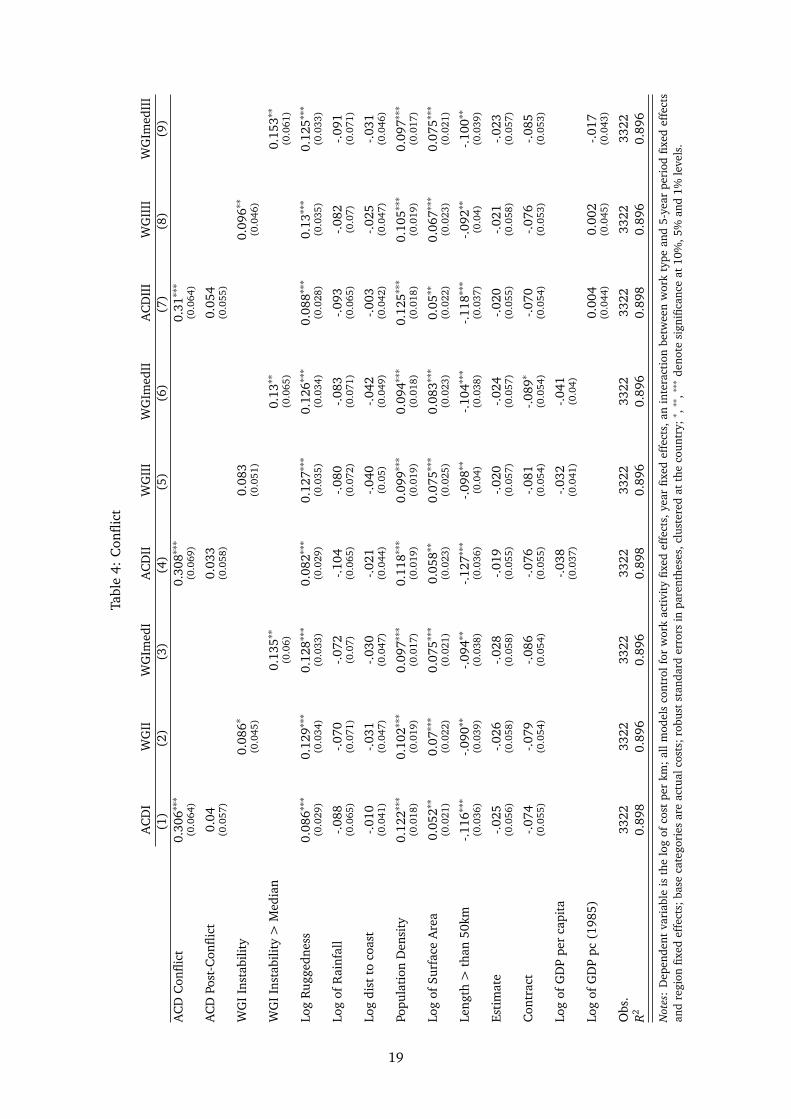
sures separately, because they are highly correlated, and the effect of conflict holding corruption
constant, and vice versa, is difficult to identify, and not the object of interest. Columns (1)-(3) in
table 4 include the conflict variables without controls for GDP per capita, columns (4)-(6) include
GDP per capita for one year before the road work activity (we refer to this as contemporaneous
GDP per capita), and columns (7)-(9) include predetermined GDP per capita in 1985. While GDP
per capita in the year of the road work activity is a more precise proxy for factor prices, it is likely to
be correlated with other contemporaneous variables affecting unit costs. Therefore, we also show
the results controlling for GDP per capita in 1985.
There is a robust and significant relationship between violent conflict and its legacy and unit
costs. Countries which are in conflict have about 30% higher unit costs. Although the coefficient on
the post-conflict dummy is positive, it is not significantly different from zero. We find evidence for
the higher costs in politically unstable countries also when using the political instability measure
from the Worldwide Governance Indicators (where we use the continuous measure as well as a
dummy variable for whether the measure is above the median of the sample). Countries which are
above the median of the sample in terms of political instability, face about 13% higher costs. The
size and significance of the coefficients is robust to omitting GDP per capita, or controlling for con-
temporaneous or predetermined GDP per capita. The magnitude of the effect appears in line with
Benamghar and Iimi (2011), who find that halving security incidents would reduce procurement
costs by 10% and cost overruns by 15%.
Unsurprisingly, geography matters. The ruggedness of the terrain in a country, surface area and
population density of a country are significantly and positively associated with unit costs. Building
a road in a more rugged terrain is likely to involve higher unit costs of construction and mainte-
nance. Column (1) suggests that a one percent increase in the ruggedness of a country is associated
with about 0.09 percent higher unit costs. The surface area and distance to the nearest ice-free
coast are collinear, so that when we include the surface area we cannot estimate the coefficient on
the distance to the nearest ice-free coast precisely anymore. The positive coefficient on the surface
area therefore is likely to pick up both the effects of being landlocked, leading to higher transport
costs, as well as the fact that perhaps constructing and maintaining roads in larger countries in-
volves higher organizational costs. Population density is also positively and significantly associated
with unit costs, indicating that unit costs rise by about ten percent for an increase of 100 people
per square kilometer. Finally, we turn to the work activity specific control variables. The estimates
suggest that there are significant economies of scale. Unit costs are about ten percent lower when
road work activities cover a length of at least 50 km. This is close to an estimate by AFRICON
(2008) who find that median unit costs are 15-20% lower for road contracts that are larger than 50
km. There is no evidence that estimated costs and actual costs are significantly different15. There is
15Unfortunately, data on the type of procurement is missing for more than half of the sample. For the unit costsfor which we have data, the procurement was done by international competitive bidding in 62%, national competitivebidding in 36%, with the remaining 26 work activities procured via single source selection, force account or limitedinternational bidding. We have also tried including a dummy variable that is equal to one if procurement was donevia international competitive bidding and zero otherwise, as well as a dummy variable that is equal to one if we missprocurement information. The results suggest that work activities awarded through an international auction have 35-38% higher costs (significant at the 5 percent level) compared to national bidding process, single source selection or
17

some evidence that contracted and estimated costs are lower than actual costs, but the effect is not
significantly different from zero.
We now turn to corruption in table 5. As before, columns (1)-(3) exclude the control for GDP
per capita, columns (4)-(6) include contemporaneous GDP per capita, and columns (7)-(9) include
the lagged GDP per capita. The pattern is consistent for the corruption variables from Transparency
International and the Worldwide Governance Indicators. We find that Transparency International’s
measure of corruption is significantly correlated with unit costs, so that a one point increase in
corruption on a ten-point scale is associated with an increase in costs by about 6-7%. The WGI
measure suggests that moving a country from the 75th percentile of corruption to the 25th per-
centile of corruption is associated with 6.3% lower unit costs. Unit costs in countries with a level
of corruption above the median as measured by the Worldwide Governance Indicator indicator of
corruption have on average 12% higher costs16. The effects of the other control variables are stable
when comparing their coefficients and standard errors with table 4.
Table 21 in the appendix shows a model without controls for conflict and corruption, and some
of the omitted controls which are still of interest. Pilot countries have on average lower costs, but
the coefficient is not significantly different from zero. There is substantial regional variation. Unit
costs in East Asia and the Pacific, Latin America and the Carribean, the Middle East and North
Africa, and South Asia are all significantly lower than in costs in the base category, Sub-Saharan
Africa. These differences in costs range between the 49% lower costs in East Asia and the Pacific,
to 18% lower costs in Latin America and the Caribbean. Subsequently, we use column (1) of table
21 to explore omitted variables.
force account. Alexeeva et al. (2008) find, when analyzing 109 contracts in 13 Sub-Saharan African countries, that localfirms have a cost advantage over international firms, likely due to lower management and overhead costs. However, localfirms perform worse in the implementation of the project, including longer delays and higher cost overruns. We do nothave data related to the implementation of the project, so we cannot test whether we find the same with our data.
16We also tested whether estimated or contracted costs are significantly lower compared to actual costs in countrieswhich suffer from conflicts, or countries with high levels of corruption, but we do not find any evidence for this.
18
Tabl
e4:
Con
flict
AC
DI
WG
IIW
GIm
edI
AC
DII
WG
III
WG
Imed
IIA
CD
III
WG
IIII
WG
Imed
III
(1)
(2)
(3)
(4)
(5)
(6)
(7)
(8)
(9)
AC
DC
onfli
ct0.
306∗∗∗
0.30
8∗∗∗
0.31∗∗∗
(0.0
64)
(0.0
69)
(0.0
64)
AC
DPo
st-C
onfli
ct0.
040.
033
0.05
4(0
.057
)(0
.058
)(0
.055
)
WG
IIn
stab
ility
0.08
6∗0.
083
0.09
6∗∗
(0.0
45)
(0.0
51)
(0.0
46)
WG
IIn
stab
ility>
Med
ian
0.13
5∗∗
0.13∗∗
0.15
3∗∗
(0.0
6)(0
.065
)(0
.061
)
Log
Rug
gedn
ess
0.08
6∗∗∗
0.12
9∗∗∗
0.12
8∗∗∗
0.08
2∗∗∗
0.12
7∗∗∗
0.12
6∗∗∗
0.08
8∗∗∗
0.13∗∗∗
0.12
5∗∗∗
(0.0
29)
(0.0
34)
(0.0
33)
(0.0
29)
(0.0
35)
(0.0
34)
(0.0
28)
(0.0
35)
(0.0
33)
Log
ofR
ainf
all
-.088
-.070
-.072
-.104
-.080
-.083
-.093
-.082
-.091
(0.0
65)
(0.0
71)
(0.0
7)(0
.065
)(0
.072
)(0
.071
)(0
.065
)(0
.07)
(0.0
71)
Log
dist
toco
ast
-.010
-.031
-.030
-.021
-.040
-.042
-.003
-.025
-.031
(0.0
41)
(0.0
47)
(0.0
47)
(0.0
44)
(0.0
5)(0
.049
)(0
.042
)(0
.047
)(0
.046
)
Popu
lati
onD
ensi
ty0.
122∗∗∗
0.10
2∗∗∗
0.09
7∗∗∗
0.11
8∗∗∗
0.09
9∗∗∗
0.09
4∗∗∗
0.12
5∗∗∗
0.10
5∗∗∗
0.09
7∗∗∗
(0.0
18)
(0.0
19)
(0.0
17)
(0.0
19)
(0.0
19)
(0.0
18)
(0.0
18)
(0.0
19)
(0.0
17)
Log
ofSu
rfac
eA
rea
0.05
2∗∗
0.07∗∗∗
0.07
5∗∗∗
0.05
8∗∗
0.07
5∗∗∗
0.08
3∗∗∗
0.05∗∗
0.06
7∗∗∗
0.07
5∗∗∗
(0.0
21)
(0.0
22)
(0.0
21)
(0.0
23)
(0.0
25)
(0.0
23)
(0.0
22)
(0.0
23)
(0.0
21)
Leng
th>
than
50km
-.116∗∗∗
-.090∗∗
-.094∗∗
-.127∗∗∗
-.098∗∗
-.104∗∗∗
-.118∗∗∗
-.092∗∗
-.100∗∗
(0.0
36)
(0.0
39)
(0.0
38)
(0.0
36)
(0.0
4)(0
.038
)(0
.037
)(0
.04)
(0.0
39)
Esti
mat
e-.0
25-.0
26-.0
28-.0
19-.0
20-.0
24-.0
20-.0
21-.0
23(0
.056
)(0
.058
)(0
.058
)(0
.055
)(0
.057
)(0
.057
)(0
.055
)(0
.058
)(0
.057
)
Con
trac
t-.0
74-.0
79-.0
86-.0
76-.0
81-.0
89∗
-.070
-.076
-.085
(0.0
55)
(0.0
54)
(0.0
54)
(0.0
55)
(0.0
54)
(0.0
54)
(0.0
54)
(0.0
53)
(0.0
53)
Log
ofG
DP
per
capi
ta-.0
38-.0
32-.0
41(0
.037
)(0
.041
)(0
.04)
Log
ofG
DP
pc(1
985)
0.00
40.
002
-.017
(0.0
44)
(0.0
45)
(0.0
43)
Obs
.33
2233
2233
2233
2233
2233
2233
2233
2233
22R2
0.89
80.
896
0.89
60.
898
0.89
60.
896
0.89
80.
896
0.89
6
Not
es:
Dep
ende
ntva
riab
leis
the
log
ofco
stpe
rkm
;al
lmod
els
cont
rolf
orw
ork
acti
vity
fixed
effe
cts,
year
fixed
effe
cts,
anin
tera
ctio
nbe
twee
nw
ork
type
and
5-ye
arpe
riod
fixed
effe
cts
and
regi
onfix
edef
fect
s;ba
seca
tego
ries
are
actu
alco
sts;
robu
stst
anda
rder
rors
inpa
rent
hese
s,cl
uste
red
atth
eco
untr
y;∗ ,∗∗
,∗∗∗
deno
tesi
gnifi
canc
eat
10%
,5%
and
1%le
vels
.
19

Tabl
e5:
Cor
rupt
ion
TIW
GI
WG
Imed
TIII
WG
III
WG
Imed
IITI
III
WG
IIII
WG
Imed
III
(1)
(2)
(3)
(4)
(5)
(6)
(7)
(8)
(9)
TIC
orru
ptio
n0.
063∗∗∗
0.06
2∗∗
0.07
6∗∗∗
(0.0
23)
(0.0
25)
(0.0
25)
WG
IC
orru
ptio
n0.
084∗∗
0.07
20.
101∗∗
(0.0
43)
(0.0
52)
(0.0
43)
WG
IC
orru
ptio
n>
Med
ian
0.12
2∗∗
0.11
2∗0.
142∗∗∗
(0.0
51)
(0.0
64)
(0.0
51)
Log
Rug
gedn
ess
0.13
7∗∗∗
0.14
9∗∗∗
0.14
7∗∗∗
0.13
5∗∗∗
0.14
6∗∗∗
0.14
6∗∗∗
0.13
7∗∗∗
0.15
1∗∗∗
0.15
2∗∗∗
(0.0
34)
(0.0
33)
(0.0
32)
(0.0
35)
(0.0
34)
(0.0
33)
(0.0
35)
(0.0
34)
(0.0
33)
Log
ofR
ainf
all
-.059
-.049
-.038
-.068
-.058
-.045
-.076
-.061
-.043
(0.0
7)(0
.066
)(0
.069
)(0
.071
)(0
.067
)(0
.07)
(0.0
71)
(0.0
67)
(0.0
69)
Log
dist
toco
ast
-.051
-.039
-.044
-.055
-.048
-.049
-.048
-.036
-.035
(0.0
5)(0
.048
)(0
.047
)(0
.052
)(0
.051
)(0
.05)
(0.0
5)(0
.048
)(0
.046
)
Popu
lati
onD
ensi
ty0.
09∗∗∗
0.09
8∗∗∗
0.08
9∗∗∗
0.08
7∗∗∗
0.09
6∗∗∗
0.08
8∗∗∗
0.09∗∗∗
0.09
9∗∗∗
0.09
1∗∗∗
(0.0
19)
(0.0
19)
(0.0
18)
(0.0
2)(0
.019
)(0
.019
)(0
.019
)(0
.019
)(0
.018
)
Log
ofSu
rfac
eA
rea
0.08
3∗∗∗
0.08
5∗∗∗
0.09
2∗∗∗
0.08
5∗∗∗
0.09
1∗∗∗
0.09
5∗∗∗
0.08
1∗∗∗
0.08
4∗∗∗
0.09∗∗∗
(0.0
22)
(0.0
21)
(0.0
22)
(0.0
24)
(0.0
23)
(0.0
23)
(0.0
22)
(0.0
22)
(0.0
22)
Leng
th>
than
50km
-.088∗∗
-.091∗∗
-.096∗∗
-.093∗∗
-.100∗∗
-.102∗∗∗
-.090∗∗
-.093∗∗
-.097∗∗
(0.0
38)
(0.0
38)
(0.0
38)
(0.0
39)
(0.0
39)
(0.0
39)
(0.0
4)(0
.04)
(0.0
4)
Esti
mat
e-.0
30-.0
31-.0
22-.0
25-.0
26-.0
18-.0
26-.0
28-.0
18(0
.058
)(0
.059
)(0
.058
)(0
.057
)(0
.058
)(0
.057
)(0
.058
)(0
.058
)(0
.057
)
Con
trac
t-.0
86-.0
80-.0
76-.0
87-.0
83-.0
78-.0
84-.0
78-.0
71(0
.055
)(0
.054
)(0
.053
)(0
.054
)(0
.054
)(0
.053
)(0
.053
)(0
.053
)(0
.052
)
Log
ofG
DP
per
capi
ta-.0
18-.0
38-.0
24(0
.041
)(0
.043
)(0
.047
)
Log
ofG
DP
pc(1
985)
0.00
070.
0009
0.01
7(0
.044
)(0
.045
)(0
.047
)
Obs
.33
2233
2233
2233
2233
2233
2233
2233
2233
22R2
0.89
60.
896
0.89
60.
896
0.89
60.
896
0.89
70.
896
0.89
6
Not
es:
Dep
ende
ntva
riab
leis
the
log
ofco
stpe
rkm
;al
lmod
els
cont
rolf
orw
ork
acti
vity
fixed
effe
cts,
year
fixed
effe
cts,
anin
tera
ctio
nbe
twee
nw
ork
type
and
5-ye
arpe
riod
fixed
effe
cts
and
regi
onfix
edef
fect
s;ba
seca
tego
ries
are
actu
alco
sts;
robu
stst
anda
rder
rors
inpa
rent
hese
s,cl
uste
red
atth
eco
untr
y;∗ ,∗∗
,∗∗∗
deno
tesi
gnifi
canc
eat
10%
,5%
and
1%le
vels
.
20
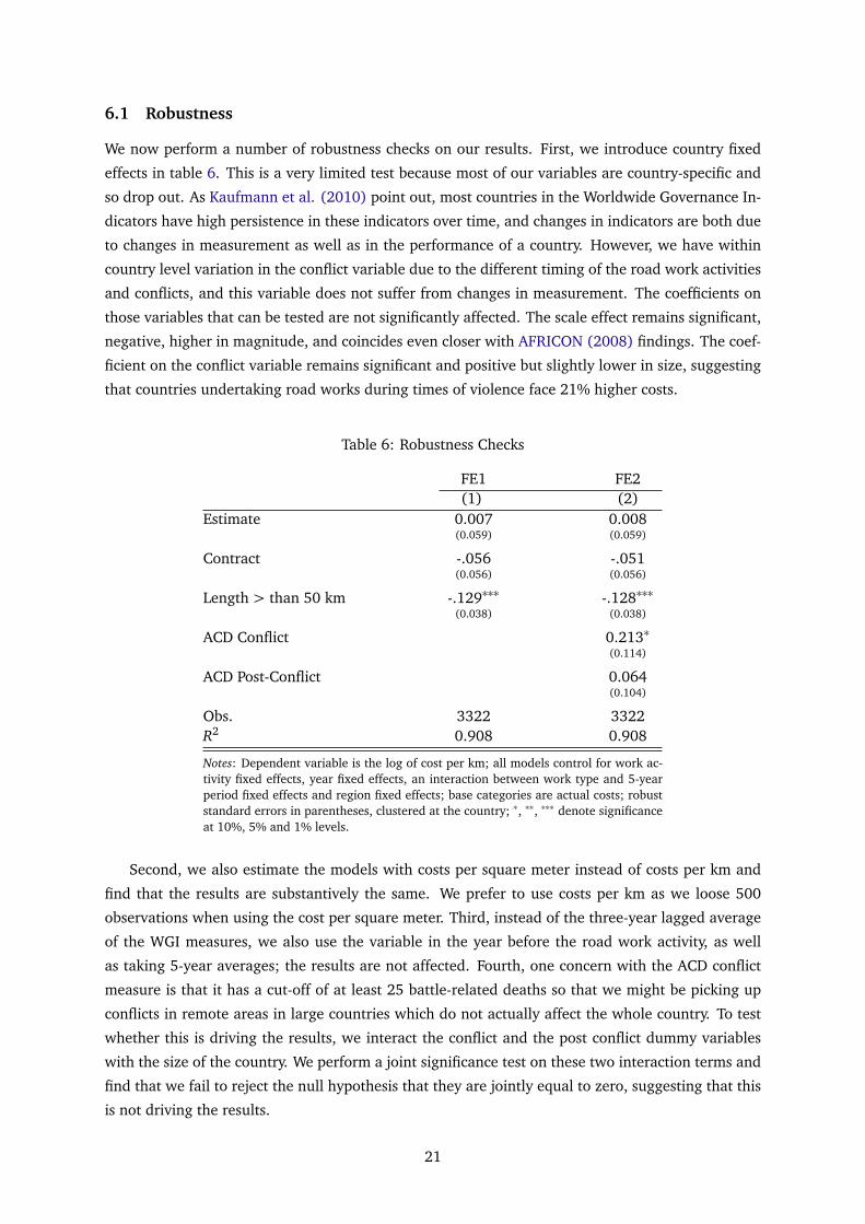
6.1 Robustness
We now perform a number of robustness checks on our results. First, we introduce country fixed
effects in table 6. This is a very limited test because most of our variables are country-specific and
so drop out. As Kaufmann et al. (2010) point out, most countries in the Worldwide Governance In-
dicators have high persistence in these indicators over time, and changes in indicators are both due
to changes in measurement as well as in the performance of a country. However, we have within
country level variation in the conflict variable due to the different timing of the road work activities
and conflicts, and this variable does not suffer from changes in measurement. The coefficients on
those variables that can be tested are not significantly affected. The scale effect remains significant,
negative, higher in magnitude, and coincides even closer with AFRICON (2008) findings. The coef-
ficient on the conflict variable remains significant and positive but slightly lower in size, suggesting
that countries undertaking road works during times of violence face 21% higher costs.
Table 6: Robustness Checks
FE1 FE2(1) (2)
Estimate 0.007 0.008(0.059) (0.059)
Contract -.056 -.051(0.056) (0.056)
Length > than 50 km -.129∗∗∗ -.128∗∗∗(0.038) (0.038)
ACD Conflict 0.213∗(0.114)
ACD Post-Conflict 0.064(0.104)
Obs. 3322 3322R2 0.908 0.908
Notes: Dependent variable is the log of cost per km; all models control for work ac-tivity fixed effects, year fixed effects, an interaction between work type and 5-yearperiod fixed effects and region fixed effects; base categories are actual costs; robuststandard errors in parentheses, clustered at the country; ∗, ∗∗, ∗∗∗ denote significanceat 10%, 5% and 1% levels.
Second, we also estimate the models with costs per square meter instead of costs per km and
find that the results are substantively the same. We prefer to use costs per km as we loose 500
observations when using the cost per square meter. Third, instead of the three-year lagged average
of the WGI measures, we also use the variable in the year before the road work activity, as well
as taking 5-year averages; the results are not affected. Fourth, one concern with the ACD conflict
measure is that it has a cut-off of at least 25 battle-related deaths so that we might be picking up
conflicts in remote areas in large countries which do not actually affect the whole country. To test
whether this is driving the results, we interact the conflict and the post conflict dummy variables
with the size of the country. We perform a joint significance test on these two interaction terms and
find that we fail to reject the null hypothesis that they are jointly equal to zero, suggesting that this
is not driving the results.
21
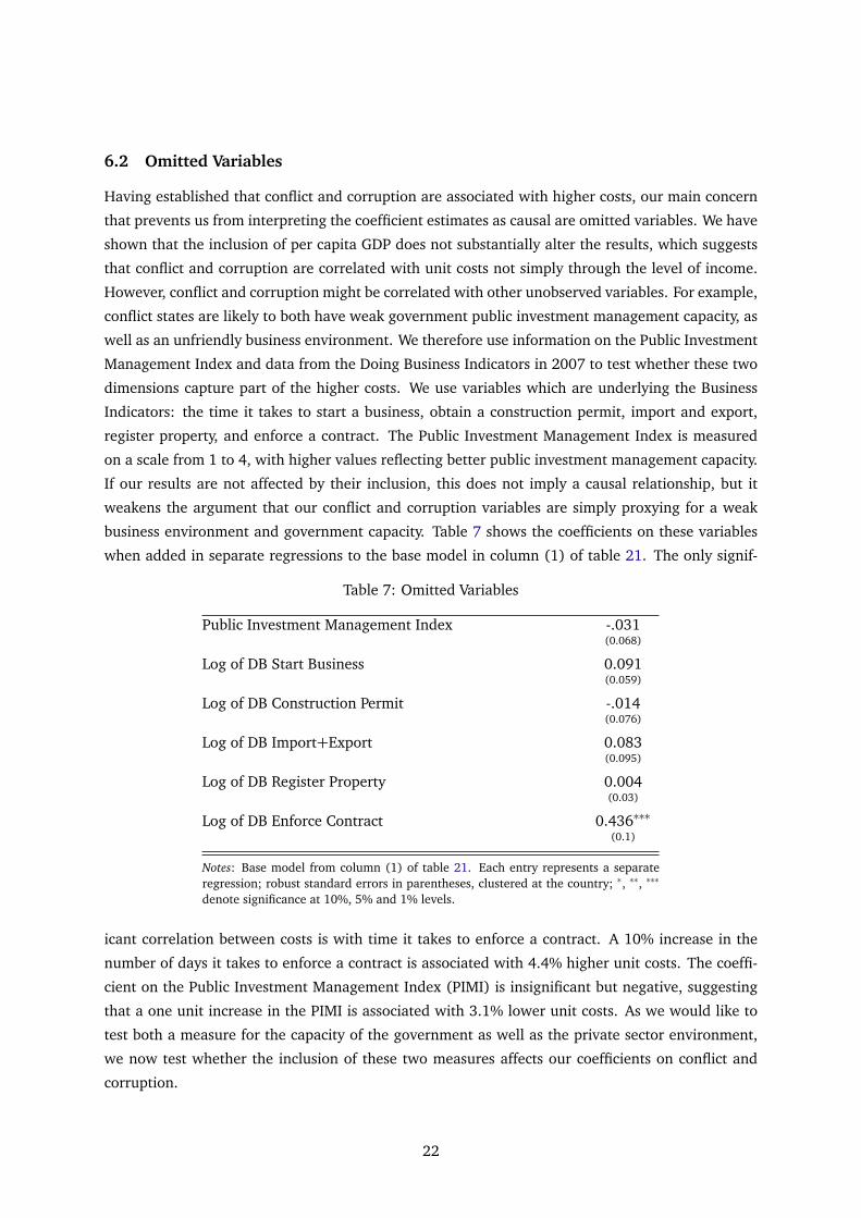
6.2 Omitted Variables
Having established that conflict and corruption are associated with higher costs, our main concern
that prevents us from interpreting the coefficient estimates as causal are omitted variables. We have
shown that the inclusion of per capita GDP does not substantially alter the results, which suggests
that conflict and corruption are correlated with unit costs not simply through the level of income.
However, conflict and corruption might be correlated with other unobserved variables. For example,
conflict states are likely to both have weak government public investment management capacity, as
well as an unfriendly business environment. We therefore use information on the Public Investment
Management Index and data from the Doing Business Indicators in 2007 to test whether these two
dimensions capture part of the higher costs. We use variables which are underlying the Business
Indicators: the time it takes to start a business, obtain a construction permit, import and export,
register property, and enforce a contract. The Public Investment Management Index is measured
on a scale from 1 to 4, with higher values reflecting better public investment management capacity.
If our results are not affected by their inclusion, this does not imply a causal relationship, but it
weakens the argument that our conflict and corruption variables are simply proxying for a weak
business environment and government capacity. Table 7 shows the coefficients on these variables
when added in separate regressions to the base model in column (1) of table 21. The only signif-
Table 7: Omitted Variables
Public Investment Management Index -.031(0.068)
Log of DB Start Business 0.091(0.059)
Log of DB Construction Permit -.014(0.076)
Log of DB Import+Export 0.083(0.095)
Log of DB Register Property 0.004(0.03)
Log of DB Enforce Contract 0.436∗∗∗(0.1)
Notes: Base model from column (1) of table 21. Each entry represents a separateregression; robust standard errors in parentheses, clustered at the country; ∗, ∗∗, ∗∗∗
denote significance at 10%, 5% and 1% levels.
icant correlation between costs is with time it takes to enforce a contract. A 10% increase in the
number of days it takes to enforce a contract is associated with 4.4% higher unit costs. The coeffi-
cient on the Public Investment Management Index (PIMI) is insignificant but negative, suggesting
that a one unit increase in the PIMI is associated with 3.1% lower unit costs. As we would like to
test both a measure for the capacity of the government as well as the private sector environment,
we now test whether the inclusion of these two measures affects our coefficients on conflict and
corruption.
22

Table 8 presents the results for conflict, where the upper panel includes the Public Investment
Management Index, and the lower panel includes the Doing Business variable measured as the log
of the number of days it takes to enforce a contract. Contemporaneous GDP per capita and lagged
GDP per capita are again added gradually to test the sensitivity of the results to its inclusion. All
models also include for the baseline controls from the previous tables.
23

Tabl
e8:
Con
flict
-Om
itte
dVa
riab
les
AC
DI
WG
IIW
GIm
edI
AC
DII
WG
III
WG
Imed
IIA
CD
III
WG
IIII
WG
Imed
III
(1)
(2)
(3)
(4)
(5)
(6)
(7)
(8)
(9)
AC
DC
onfli
ct0.
308∗∗∗
0.31
3∗∗∗
0.31
1∗∗∗
(0.0
67)
(0.0
7)(0
.066
)
AC
DPo
st-C
onfli
ct0.
038
0.03
40.
051
(0.0
6)(0
.059
)(0
.057
)
WG
IIn
stab
ility
0.08
8∗0.
089∗
0.09
8∗∗
(0.0
5)(0
.054
)(0
.049
)
WG
IIn
stab
ility>
Med
ian
0.14∗∗
0.14
3∗∗
0.16
1∗∗
(0.0
69)
(0.0
71)
(0.0
68)
Publ
icIn
vest
men
tM
anag
emen
tIn
dex
-.010
-.001
0.00
50.
006
0.01
30.
023
-.018
-.006
0.00
7(0
.055
)(0
.065
)(0
.067
)(0
.059
)(0
.068
)(0
.069
)(0
.058
)(0
.067
)(0
.069
)
Log
ofG
DP
per
capi
taN
ON
ON
OYE
SYE
SYE
SN
ON
ON
OLo
gof
GD
Ppc
(198
5)N
ON
ON
ON
ON
ON
OYE
SYE
SYE
SO
bs.
3322
3322
3322
3322
3322
3322
3322
3322
3322
R20.
898
0.89
60.
896
0.89
80.
896
0.89
60.
898
0.89
60.
896
AC
DC
onfli
ct0.
256∗∗∗
0.25
9∗∗∗
0.26
1∗∗∗
(0.0
6)(0
.064
)(0
.06)
AC
DPo
st-C
onfli
ct0.
047
0.04
0.05
7(0
.058
)(0
.059
)(0
.056
)
WG
IIn
stab
ility
0.08
2∗∗
0.08
3∗∗
0.08
9∗∗
(0.0
36)
(0.0
41)
(0.0
36)
WG
IIn
stab
ility>
Med
ian
0.11
8∗∗
0.11
5∗∗
0.13
1∗∗
(0.0
51)
(0.0
56)
(0.0
52)
Log
ofD
BEn
forc
eC
ontr
act
0.34
4∗∗∗
0.42
3∗∗∗
0.41
6∗∗∗
0.34
8∗∗∗
0.42
8∗∗∗
0.42
1∗∗∗
0.32
5∗∗∗
0.40
2∗∗∗
0.39
5∗∗∗
(0.0
81)
(0.0
87)
(0.0
88)
(0.0
83)
(0.0
89)
(0.0
9)(0
.084
)(0
.091
)(0
.093
)
Log
ofG
DP
per
capi
taN
ON
ON
OYE
SYE
SYE
SN
ON
ON
OLo
gof
GD
Ppc
(198
5)N
ON
ON
ON
ON
ON
OYE
SYE
SYE
SO
bs.
3322
3322
3322
3322
3322
3322
3322
3322
3322
R20.
899
0.89
80.
898
0.89
90.
898
0.89
80.
899
0.89
80.
898
Not
es:
Dep
ende
ntva
riab
leis
the
log
ofco
stpe
rkm
;al
lmod
els
cont
rolf
orw
ork
acti
vity
fixed
effe
cts,
year
fixed
effe
cts,
anin
tera
ctio
nbe
twee
nw
ork
type
and
5-ye
arpe
riod
fixed
effe
cts
and
regi
onfix
edef
fect
s,du
mm
yva
riab
les
for
actu
alan
dco
ntra
cted
cost
s,ty
peof
terr
ain,
rugg
edne
ss,d
ista
nce
toth
ene
ares
tice
-fre
eco
ast,
popu
lati
onde
nsit
y,lo
gof
surf
ace
area
,dum
my
for
leng
ht>
50km
;rob
ust
stan
dard
erro
rsin
pare
nthe
ses,
clus
tere
dat
the
coun
try;∗ ,∗∗
,∗∗∗
deno
tesi
gnifi
canc
eat
10%
,5%
and
1%le
vels
.
24

The coefficient on the Public Investment Management Index is never significantly different from
zero and it’s inclusion does not affect the size and significance of the conflict variables. The business
environment reveals a more consistent correlation with road works costs. A 10% increase in the
number of days it takes to enforce a contract, is associated with a 2-4% increase in unit costs, and
the results are robust to including contemporaneous and lagged GDP per capita or excluding GDP
per capita. Its inclusion slightly reduces the size of the conflict variables. The most direct measure
of conflict from the ACD drops in size from a premium of 30.6% to 25.6% in column (1) when ac-
counting for the business environment. The Worldwide Governance Indicator measure also slightly
drops in size from 14% higher costs for countries above the median of political instability to 12%
in column (3). The results are not sensitive to the inclusion of contemporaneous or lagged GDP per
capita.
Table 9 shows the same exercise for corruption. Both the inclusion of the Public Investment
Management Index and the Doing Business variable do not substantively affect the size nor the
significance of the coefficients, suggesting that there is a significant association with corruption
after controlling for the business environment and the public investment capacity. Overall, the find-
ings suggest that our measure of the business environment explains some of the premium charged
by firms operating in conflict countries with little effect of either of the two measures on corruption.
25

Tabl
e9:
Cor
rupt
ion
-Om
itte
dVa
riab
les
TIW
GI
WG
Imed
TIII
WG
III
WG
Imed
IITI
III
WG
IIII
WG
Imed
III
(1)
(2)
(3)
(4)
(5)
(6)
(7)
(8)
(9)
TIC
orru
ptio
n0.
062∗∗∗
0.06
2∗∗
0.07
6∗∗∗
(0.0
24)
(0.0
25)
(0.0
25)
WG
IC
orru
ptio
n0.
076∗
0.06
80.
093∗∗
(0.0
44)
(0.0
51)
(0.0
44)
WG
IC
orru
ptio
n>
Med
ian
0.12∗∗
0.11
3∗0.
138∗∗∗
(0.0
53)
(0.0
64)
(0.0
53)
Publ
icIn
vest
men
tM
anag
emen
tIn
dex
-.014
-.025
-.005
-.007
-.014
0.00
2-.0
19-.0
30-.0
12(0
.063
)(0
.064
)(0
.064
)(0
.067
)(0
.066
)(0
.066
)(0
.066
)(0
.066
)(0
.066
)
Log
ofG
DP
per
capi
taN
ON
ON
OYE
SYE
SYE
SN
ON
ON
OLo
gof
GD
Ppc
(198
5)N
ON
ON
ON
ON
ON
OYE
SYE
SYE
SO
bs.
3322
3322
3322
3322
3322
3322
3322
3322
3322
R20.
896
0.89
60.
896
0.89
60.
896
0.89
60.
897
0.89
60.
896
TIC
orru
ptio
n0.
06∗∗∗
0.06
2∗∗∗
0.07∗∗∗
(0.0
2)(0
.023
)(0
.021
)
WG
IC
orru
ptio
n0.
096∗∗
0.09
3∗0.
108∗∗
(0.0
42)
(0.0
53)
(0.0
43)
WG
IC
orru
ptio
n>
Med
ian
0.13∗∗∗
0.12
7∗∗
0.14
5∗∗∗
(0.0
48)
(0.0
6)(0
.049
)
Log
ofD
BEn
forc
eC
ontr
act
0.42
5∗∗∗
0.44
2∗∗∗
0.44
2∗∗∗
0.42
9∗∗∗
0.44
6∗∗∗
0.44
6∗∗∗
0.39
6∗∗∗
0.42
3∗∗∗
0.42∗∗∗
(0.0
92)
(0.0
97)
(0.1
02)
(0.0
93)
(0.0
99)
(0.1
04)
(0.0
95)
(0.1
01)
(0.1
05)
Log
ofG
DP
per
capi
taN
ON
ON
OYE
SYE
SYE
SN
ON
ON
OLo
gof
GD
Ppc
(198
5)N
ON
ON
ON
ON
ON
OYE
SYE
SYE
SO
bs.
3322
3322
3322
3322
3322
3322
3322
3322
3322
R20.
898
0.89
80.
898
0.89
80.
898
0.89
80.
898
0.89
80.
898
Not
es:
Dep
ende
ntva
riab
leis
the
log
ofco
stpe
rkm
;al
lmod
els
cont
rolf
orw
ork
acti
vity
fixed
effe
cts,
year
fixed
effe
cts,
anin
tera
ctio
nbe
twee
nw
ork
type
and
5-ye
arpe
riod
fixed
effe
cts
and
regi
onfix
edef
fect
s,du
mm
yva
riab
les
for
actu
alan
dco
ntra
cted
cost
s,ty
peof
terr
ain,
rugg
edne
ss,d
ista
nce
toth
ene
ares
tice
-fre
eco
ast,
popu
lati
onde
nsit
y,lo
gof
surf
ace
area
,dum
my
for
leng
ht>
50km
;rob
ust
stan
dard
erro
rsin
pare
nthe
ses,
clus
tere
dat
the
coun
try;∗ ,∗∗
,∗∗∗
deno
tesi
gnifi
canc
eat
10%
,5%
and
1%le
vels
.
26

6.3 How do Costs affect Provision?
The core of this paper has been to investigate the relationship between unit costs, conflict and
corruption. Finally, we investigate whether higher unit costs are associated with lower outcomes
as measured by the log of kilometers of roads paved per person and the performance of a country
in the quality of trade and transport related infrastructure index which as measured between one
and five17 (Arvis et al. 2007). As road work activities are heterogenous, we first want to net out
variation that is related to the road work activity, time effects as well as region fixed effects. We
can then use the residual of this cost regression as a measure of residual unit costs and use it as
a control in a regression of provision on unit costs, and a vector of controls. We prefer to directly
estimate the coefficient by regressing the outcome measure on unit costs, while controlling for the
vector of controls employed in the baseline regression in column (1) of table 21. Table 10 shows
Table 10: Correlation between Unit Costs and Infrastructure Provision
pavedroad infrastructure(1) (2)
Log of Cost per km (2000 US$) -.068∗∗ -.042∗∗(0.028) (0.017)
Obs. 3322 3269R2 0.681 0.668
Notes: Dependent variable as follows: log of km of paved road per person in column(1); quality of trade and transport related infrastructure index in column (2); bothequations include all controls employed in column (1) of table 21; standard errorsare clustered at the country level; ∗, ∗∗, ∗∗∗ denote significance at 10%, 5% and 1%levels.
the correlation between unit costs and transport infrastructure outcomes. We find evidence that
higher costs are associated with a worse infrastructure. A ten percent increase in unit costs is
associated with a 0.68% reduction in the kilometers of paved roads per person in a country and a
0.4 reduction in the quality of trade and transport related infrastructure index component of the
logistics performance index. At the median value (2.23) this change corresponds to a move almost
into the top quartile. The regression in table 10 includes the same controls as column (1) of table
21, but the results remain the same when we control for contemporaneous per capita GDP or per
capita GDP in 1985.
6.4 Future Research
This section reviews our core results and discusses avenues for further research, drawing on some
recommendations outlined in World Bank (2011a). First, one possible area of future research is
to examine the mechanisms through which state fragility affects costs. In this paper, we modeled
this in the cost function as a premium that firms require to cover costs due to disruption and risk.
However, an alternative explanation is that fewer firms are left in the market after conflicts as they
get driven out of business; if the supply of firms providing road works decreases by more than the
contraction of demand, this will lead to higher prices. In this context, a combination of insuring
17The measure is continuous and bounded between one and five.
27

risks of construction firms in fragile states and lifting of constraints to firms entering the construc-
tion sector might be helpful to increase competition and to reduce unit costs. Little is known also
about the evolution of prices in post-conflict settings when investment accelerates so that there is
increased pressure on the construction sector, foreign companies are eager to enter the new market
and there might be delays in tendering due to aid conditionalities18. Here the effect is ambiguous:
if the growth in demand outstrips the growth in supply, prices will increase; if large foreign com-
panies, which are able to operate on losses in the short run, undercut prices in order to enter a
market, this might even lead to lower prices.
Second, our results present evidence that there is a correlation between corruption and unit
costs and our simple theoretical framework assumed that this is due to bribe payments to officials
to obtain permits. A main drawback of perception based measures is that they might reflect over-
all governance quality of a country rather than being specifically related to the level of corruption
(Kenny 2009). Olken (2009) finds that for road projects in Indonesia, although perceptions are
correlated with his estimate for corruption, the correlation is fairly weak. Country level percep-
tion measures also do not allow us to distinguish between the levels of corruption across different
sectors, petty corruption vs grand corruption, cartellization of the industry, or misreporting of ex-
penditures. Sector specific measures of corruption from firm level surveys would allow establishing
a tighter link between corruption and unit costs of transport infrastructure as well as the extent of
corruption.
Missing expenditures and inferior inputs are a serious concern not only affecting the cost of
construction but also subsequent maintenance costs for the government. For example, an audit of
18 road contracts by the Government of Zambia found that 50% of samples used weaker cement
than required, 75% of samples had more clay content than required and all samples indicated use
of substandard cement (Government of Zambia 2010). To our knowledge, the only study that sys-
tematically tests ways to reduce missing expenditures in the context of the roads sector is Olken
(2007), who finds that increasing the audit probability by the government from 4 to 100% reduced
missing expenditures by 8%. The audit treatment was significantly more effective than increasing
community participation in the monitoring process. However, he also finds that in villages that
were exposed to the audit experiment, a higher number of jobs was given to family members of
project officials, suggesting that corruption might have been shifted. World Bank (2011a) suggest
alternative mechanisms, including strengthening the Engineer19 and checking the wealth of key
procurement agency officials. We are not aware of evidence on the effectiveness of these vari-
ous policies. Countries could also experiment with different incentive contracts for the engineer
to incentivize reporting of corruption and fraud, as well as recruitment of the engineer based on
reputation of honesty rather than simply based on price. The collection of a sample of each con-
tracted road work activity by an engineer to estimate costs and verify contracted materials could
18The issues associated with the positive demand shock also apply to countries experiencing windfalls from naturalresources that trigger spending booms.
19Projects financed by the World Bank usually require an Engineer, who takes on the supervision of the contractor(World Bank 2012); for larger projects this can be a supervisory firm. The Engineer is an expert in the design of theproject and expected to oversee the complete implementation, ensuring that quality and implementation are as stipulatedin the contract (World Bank 2011a).
28

be part of a construction contract. Countries could then experiment with these various policies at a
sub-national level to investigate their effectiveness in reducing missing expenditures and the use of
substandard materials.
Third, an important area this paper did not tackle due to data limitations is the market struc-
ture of the local construction industry and collusion among construction sector firms20. World Bank
(2011a) estimate that the overcharge due to cartels leads to about 40% higher prices on average in
developing countries. Given the magnitude of these effects, limiting collusion is a first order concern
to ensure efficiency of public spending. The report highlights that cartellization of the construction
sector is not distinctive to developing countries: cartels in the roads and construction sector were
found in the United states, Denmark, France, Germany, Japan and Sweden21. This does not imply
that governments in developing countries with weaker detection technologies should give up on
detecting collusion, but it is important to keep in mind that this is a problem when government
capacity is high. World Bank (2011a) suggest a fairly simple first step is to detect collusion using
statistical models for every auction that takes place (Porter and Zona 1993; Bajari and Ye 2003).
To our knowledge, there is no quantitative evidence on different policies to combat collusion in the
context of the construction sector in low income countries.
Higher transparency in the construction sector has been advocated as one way to combat col-
lusion. An example for this is the Construction Sector Transparency Initiative (CoST), funded by
the German Agency for International Cooperation, the United Kingdom’s Department for Interna-
tional Development, and the World Bank which has been piloted in Tanzania, Zambia, Malawi,
Vietnam, the Philippines, Ethiopia and the United Kingdom (Construction Sector Transparency Ini-
tiative 2011). Building up databases of unit costs of comparable activities will certainly assist
governments in ensuring that they are not overpaying. However, there are trade-offs between pub-
lication of estimated costs and collusion. While the publishing cost estimates reduced average bids
and left the size of the winning bid unchanged in auctions in Oklahoma, evidence from an Eastern
European country showed that it led to bids almost exactly tracing the estimated costs suggesting
that higher transparency helped companies collude (Silva et al. 2008; World Bank 2011a).
Third, this paper finds that the time it takes to enforce a contract is significantly correlated with
costs. One interpretation of this finding is that the time it takes to enforce a contract reflects the
strength of legal institutions in a country. If relational contracts allow the buyer to efficiently con-
tract when courts are weak, but road contracts are allocated via a one stage sealed bid auction inde-
pendent of the strength of the court system, governments in countries with weak law enforcement
pay higher prices. Banerjee and Duflo (2000) argue that reputation is an important determinant
of contracting outcomes for firms in the Indian software industry. Johnson et al. (2002) find that
when courts are weak, firms which purchase customized products state that they would prefer to
20Data and analysis on market structure are scattered, for example see Lan (2010) for China and ? for Nigeria; (Ofori2007) underlines that in addition to the inadequate knowledge of the market structure of the local construction industryin developing countries, little attention has been given to the contribution of the informal sector to construction.
21See Hüschelrath et al. (2010) for a study on the road surfacing cartel in Switzerland, as well as a discussion of casesof cartels in Austria (Asphalt Mixing Plant), Netherlands (Bitumen), Finland (Asphalt) and Sweden (Asphalt).
29

keep the contract with their existing supplier when offered a 10% lower price from a new supplier.
This highlights another trade-off, between fostering competition and rewarding good behavior of
firms. Findings from the initial pilots under the Construction Sector Transparency Initiative showed
that cost overruns in the sample of 145 contracts amount to 58% in Ethiopia, 35% in Vietnam,
10% in the Philippines and 6% in the United Kingdom, suggesting that hold up problems are of a
significant magnitude. If construction firms could be compensated for good behavior by awarding
future contracts to them, this could reduce hold-up problems, but decreases competition. One step
towards increasing reputational concerns of firms is the World Bank Integrity Vice Presidency’s de-
barment of 405 companies, non-governmental organizations and individuals22. These entities are
listed on the website of the World Bank, including on which grounds they were debarred and the
duration of ineligibility, thereby lowering their payoff from defecting.
This implies that there is scope for research into how companies which are honest and deliver
efficiently could be rewarded positively, while not sacrificing competition. Krasnokutskaya and
Seim (2011) evaluate the effects of a bid preference programs for small firms bidding for highway
projects in California and find that the preference program significantly affects firms decisions to
submit bids, and raises project costs between 1.5-2.3% once endogenous entry to bid is taken into
account. To reduce time overruns (amounting to 130% in Ethiopia, 106% in Tanzania and 97% in
Malawi (Construction Sector Transparency Initiative 2011)), Lewis and Bajari (2011) suggest score
based auctions which are designed to internalize the costs of time overruns to construction sector
firms.
Fifth, this paper was agnostic about the costs of inputs into production, such as equipment,
raw materials, as well as human resources. Information on input prices would allow a better under-
standing of which part of the premium experienced in conflict and corrupt countries is due to higher
input prices, and which part is due to rents obtained by firms undertaking the road work activities.
Cartels do not only take place on the construction firm side, but also on the input side. For example,
Hüschelrath et al. (2013) finds that cement prices dropped by 25% higher following the break-up
of the German cement cartel. The construction sector PPP of the International Comparison Project
2011 has collected detailed information on a range of comparable input prices, which could be used
as a first step to explore differences in unit costs across countries23.
Finally, this paper and the main discussion was centered on transport infrastructure. A better
understanding of unit costs of construction of other types of projects, for example, residential and
commercial housing, is another avenue for further research. Advances in the methodology to mea-
sure unit costs are a prerequisite to understand differences in costs, so efforts should focus both on
measurement as well as the analysis.
22As of 25 March 2013, list available under www.worldbank.org/integrity.23To our knowledge, the data will be released in June 2013.
30

7 Conclusion
This paper presented a first systematic analysis of drivers of unit costs across countries. Our analysis
yielded five main findings. First, we showed that there is a large dispersion in unit costs across
countries for comparable road work activities. For example, the difference between countries of an
asphalt overlay of 40 to 59 mm amounts to a factor of three to four. Second, we found that after
accounting for environmental drivers of costs such as terrain ruggedness and proximity to markets,
residual unit costs are significantly higher in fragile countries. Countries which are in conflict
have about 30% higher unit costs. This result is robust across a range of measures of conflict and
political instability. Third, we also find evidence that costs are higher in countries with higher levels
of corruption. Countries with corruption levels as measured by the World Governance Indicators
above the median in the sample have about 12% higher costs. Given that corruption and collusive
practices might be even higher for projects undertaken directly by governments without the need
to respect procurement procedures of the World Bank, the higher costs in corrupt environments are
potentially a lower bound of the estimate. Fourth, the premium charged by firms in conflict and
corrupt countries remains when we control for the government’s public investment capacity and
the business environment. Finally, we found that higher unit costs are significantly associated with
lower levels of infrastructure provision. Based on these findings, we laid out a research agenda.
31

References
AFRICON (2008). Unit costs of infrastructure projects in sub-saharan africa, africa infrastruc-
ture country diagnostic. Background Paper No. 11 (Phase I) Africa Infrastructure Country
Diagnostic, The World Bank.
Ahmed, F. Z. (2012). Remittances deteriorate governance. Review of Economics and Statistics (0).
Alesina, A. and B. Weder (2002). Do corrupt governments receive less foreign aid? The American
Economic Review 92(4), 1126–1137.
Alexeeva, V., C. Queiroz, and S. Ishihara (2008). Monitoring road works contracts and unit costs
for enhanced governance in sub-saharan africa. Technical report.
Alexeeva, V., C. Queiroz, and S. Ishihara (2011). Monitoring road works contracts and unit costs
for enhanced governance in europe and central asia. Technical report.
Arvis, J.-F., M. Mustra, L. Ojala, T. Naula, and J. Panzer (2007). Connecting to compete - trade
logistics in the global economy: The logistics performance index and its indicators.
Bajari, P. and L. Ye (2003). Deciding between competition and collusion. Review of Economics
and Statistics 85(4), 971–989.
Bandiera, O., A. Prat, and T. Valletti (2009). Active and passive waste in government spending:
Evidence from a policy experiment. The American Economic Review 99(4), 1278–1308.
Banerjee, A., S. Mullainathan, and R. Hanna (2012). Corruption chapter full 17. NBER Working
Paper (w17968).
Banerjee, A. V. and E. Duflo (2000). Reputation effects and the limits of contracting: A study of
the indian software industry. The Quarterly Journal of Economics 115(3), 989–1017.
Benamghar, R. and A. Iimi (2011). Efficiency in public procurement in rural road projects of
nepal. World bank policy research working paper series 5736.
Blattman, C. and E. Miguel (2010). Civil war. Journal of Economic Literature 48(1), 3–57.
Board, S. (2011). Relational contracts and the value of loyalty. American Economic Re-
view 101(7), 3349.
Buys, P., U. Deichmann, and D. Wheeler (2010). Road network upgrading and overland trade
expansion in sub-saharan africa. Journal of African Economies 19(3), 399–432.
Compte, O., A. Lambert-Mogiliansky, and T. Verdier (2005). Corruption and competition in pro-
curement auctions. Rand Journal of Economics, 1–15.
Construction Sector Transparency Initiative (2011). Report on baseline studies: International
comparison. Technical report, Construction Sector Transparency Initiative.
Dabla-Norris, E., J. Brumby, A. Kyobe, Z. Mills, and C. Papageorgiou (2011). Investing in public
investment: an index of public investment efficiency. Technical report.
Dell, M., B. F. Jones, and B. A. Olken (2012). Temperature shocks and economic growth: Evi-
dence from the last half century. American Economic Journal: Macroeconomics 4(3), 66–95.
32

Dercon, S., D. O. Gilligan, J. Hoddinott, and T. Woldehanna (2009). The impact of agricultural
extension and roads on poverty and consumption growth in fifteen ethiopian villages. Amer-
ican Journal of Agricultural Economics 91(4), 1007–1021.
Di Tella, R. and E. Schargrodsky (2003). The role of wages and auditing during a crackdown on
corruption in the city of buenos aires. Journal of Law and Economics 46(1), 269–292.
Donaldson, D. (2012). Railroads of the raj: Estimating the impact of transportation infrastruc-
ture. Technical report.
Estache, A. and A. Iimi (2009). Joint bidding, governance and public procurement costs: a case
of road projects. Annals of Public and Cooperative Economics 80(3), 393–429.
Estache, A. and A. Iimi (2010). Bidder asymmetry in infrastructure procurement: Are there any
fringe bidders? Review of Industrial Organization 36(2), 163–187.
Fisman, R. and E. Miguel (2007). Corruption, norms, and legal enforcement: Evidence from
diplomatic parking tickets. Journal of Political Economy 115(6), 1020–1048.
Flyvbjerg, B., M. K. Skamris Holm, and S. L. Buhl (2003). How common and how large are cost
overruns in transport infrastructure projects? Transport Reviews 23(1), 71–88.
Gleditsch, N., P. Wallensteen, M. Eriksson, M. Sollenberg, and H. Strand (2002). Armed conflict
1946-2001: A new dataset. Journal of peace research 39(5), 615–637.
Government of Zambia (2010). Report of the auditor gerneral on the road development agency
for the period january 2006 to sepetmber 2009. Technical report, Government of Zambia.
Graf Lambsdorff, J. (2005). Determining trends for perceived levels of corruption. Technical
report, Passauer Diskussionspapiere: Volkswirtschaftliche Reihe.
Greene, W. H. (2003). Econometric analysis, Volume 5. Prentice hall Upper Saddle River, NJ.
Hüschelrath, K., N. Leheyda, and P. Beschorner (2010). Assessing the effects of a road-surfacing
cartel in switzerland. Journal of Competition Law and Economics 6(2), 335–374.
Hüschelrath, K., K. Müller, and T. Veith (2013). Concrete shoes for competition: The effect of
the german cement cartel on market price. Journal of Competition Law and Economics 9(1),
97–123.
Huysentruyt, M. (2011). Development aid by contract: Outsourcing and contractor identity.
mimeo.
Hyytinen, A., S. Lundberg, and O. Toivanen (2007). Politics and procurement: Evidence from
cleaning contracts. Technical report.
Jacoby, H. G. and B. Minten (2009). On measuring the benefits of lower transport costs. Journal
of Development Economics 89(1), 28–38.
Johnson, S., J. McMillan, and C. Woodruff (2002). Courts and relational contracts. Journal of
Law, Economics, and Organization 18(1), 221–277.
Kaufmann, D., A. Kraay, and M. Mastruzzi (2010). The worldwide governance indicators:
methodology and analytical issues. World Bank Policy Research Working Paper (5430).
33
Kenny, C. (2009). Measuring corruption in infrastructure: Evidence from transition and devel-
oping countries. The Journal of Development Studies 45(3), 314–332.
Khandker, S. R., Z. Bakht, and G. B. Koolwal (2009). The poverty impact of rural roads: evidence
from bangladesh. Economic Development and Cultural Change 57(4), 685–722.
Krasnokutskaya, E. and K. Seim (2011). Bid preference programs and participation in highway
procurement auctions. The American Economic Review 101(6), 2653–2686.
Lan, L. (2010). The Expansion of Chinese Construction Companies in the Global Market. Ph. D.
thesis, University of Kansas School of Engineering.
Lewis, G. and P. Bajari (2011). Procurement contracting with time incentives: Theory and evi-
dence. The Quarterly Journal of Economics 126(3), 1173–1211.
Li, T. and X. Zheng (2009). Entry and competition effects in first-price auctions: Theory and
evidence from procurement auctions. The Review of Economic Studies 76(4), 1397–1429.
Limao, N. and A. J. Venables (2001). Infrastructure, geographical disadvantage, transport costs,
and trade. The World Bank Economic Review 15(3), 451–479.
Miguel, E., S. Satyanath, and E. Sergenti (2004). Economic shocks and civil conflict: An instru-
mental variables approach. Journal of Political Economy, 725–753.
Moavenzadeh, F. (1978). Construction industry in developing countries. World Develop-
ment 6(1), 97–116.
Mu, R. and D. van de Walle (2011). Rural roads and local market development in vietnam. The
Journal of Development Studies 47(5), 709–734.
Nunn, N. and D. Puga (2012). Ruggedness: The blessing of bad geography in africa. Review of
Economics and Statistics 94(1), 20–36.
Ofori, G. (2007). Construction in developing countries. Construction Management and Eco-
nomics 25(1), 1–6.
Olken, B. A. (2007). Monitoring corruption: Evidence from a field experiment in indonesia.
Journal of Political Economy 115(2).
Olken, B. A. (2009). Corruption perceptions vs. corruption reality. Journal of Public Eco-
nomics 93(7), 950–964.
Olken, B. A. and R. Pande (2012). Corruption in developing countries. Annu. Rev. Econ. 4(1),
479–509.
Pesendorfer, M. (2000). A study of collusion in first-price auctions. The Review of Economic Stud-
ies 67(3), 381–411.
Porter, R. H. and J. D. Zona (1993). Detection of bid rigging in procurement auctions. Journal of
Political Economy 101(3), pp. 518–538.
Rebosio, M. and P. E. Wam (2011). Violent conflict and the road sector: Points of interaction.
Technical report, The World Bank.
34

Shiferaw, A., M. Soederbom, E. Siba, and G. Alemu (2011). Road networks and enterprise per-
formance in ethiopia: Evidence from the road sector development program. IGC Working
Paper 12/0696.
Silva, D. G. D., T. Dunne, A. Kankanamge, and G. Kosmopoulou (2008). The impact of public
information on bidding in highway procurement auctions. European Economic Review 52(1),
150 – 181.
Stifel, D., B. Minten, and B. Koro (2012). Economic benefits and returns to rural feeder roads:
Evidence from a quasi-experimental setting in ethiopia. ESSP II Working Paper 40.
Svensson, J. (2005). Eight questions about corruption. The Journal of Economic Perspec-
tives 19(3), 19–42.
Teravaninthorn, S. and G. Raballand (2009). Transport Prices and Costs in Africa: A Review of the
Main International Corridors, Volume 772. World Bank Publications.
Themnér, L. and P. Wallensteen (2012). Armed conflicts, 1946–2011. Journal of Peace Re-
search 49(4), 565–575.
Thompson, T. and A. Shah (2005). Transparency internationalŠs corruption perceptions index:
Whose perceptions are they anyway? Technical report.
Transparency International (2011). Bribe payer’s index 2011.
Treisman, D. (2007). What have we learned about the causes of corruption from ten years of
cross-national empirical research? Annu. Rev. Polit. Sci. 10, 211–244.
Wei, S.-J. (2000). How taxing is corruption on international investors? Review of economics and
statistics 82(1), 1–11.
World Bank (2006). Road Costs Knowledge System (ROCKS) Version 2.3 User’s Guide. Transport
and Urban Development Department, The World Bank.
World Bank (2011a). Curbing fraud, corruption, and collusion in the roads sector. Integrity Vice
Presidency.
World Bank (2011b). World development report 2011: Conflict, Security and Development. Wash-
ington, DC: World Bank.
World Bank (2012). Procurement of works & userŠs guide. Standard bidding documents.
Zitzewitz, E. (2012). Forensic economics. Journal of Economic Literature 50(3), 731–69.
35

8 Appendix
8.1 Data Sources for Additional Variables
8.1.1 Exchange Rate and Consumer Price Index
As the database does not contain consumer price indices and exchange rates after 2004, we re-
calculate all conversions using the official exchange rate (LCU per US$, period average) and the
consumer price index from the World Development Indicators 2012. Projects denominated in cur-
rencies other than US$ were first deflated or inflated to the reference year 2000, and then converted
into US$. Projects denominated in US$ were deflated to the reference year 2000 using the consumer
price index of the United States. The costs are very similar to the ones provided in the database,
with 93% (91%) of costs per km (square meter) lying within 2% of the original data provided24.
8.1.2 Ruggedness
Our measure of ruggedness is taken from Nunn and Puga (2012) which in turn is based on Riley et
al (1999). It represents the average ruggedness of a country and is measured in hundreds of meters
of elevation difference for grid points about 926 meters apart. The lowest level of ruggedness is in
Mauritania with an index of 0.115, and the highest is Bhutan, with an index of 6.740.
8.1.3 Rainfall
Our measure for rainfall is taken from Dell et al. (2012) and is defined as population weighted
country level precipitation in 100s millimeters.
8.1.4 Basic Socio-economic Data
For the total population, total surface area, and GDP per capita for each country we use the World
Development Indicators.
8.1.5 Public Sector Management Capacity
To measure the capacity of the public sector to execute projects we use the Public Investment Man-
agement Index (PIMI) collected by Dabla-Norris et al. (2011). The Public Investment Management
Index is measured on a scale from 0 to 4.
8.1.6 The Business Environment
To measure the business environment of the country, we use data from the Doing Business Indica-
tors in 2007 and measure costs in terms of time the number it takes to enforce a contract. We use
2007 because this is the first year for which we have complete coverage.
24Azerbeijan, Ghana and Venezuela devalued their currencies since 2000, so for these countries we use the unit costdata provided in the database.
36

Tables 11 shows the descriptive statistics of the control variables. Some variables are not avail-
able for the year of the construction project. We therefore distinguish between the following cases:
first, if the variable is only available at one point of time we assign the available value to the con-
struction project; second, if the variable is available for at least two years we distinguish between
the following three cases: (i) when the construction project took place before the year the variable
becomes available, we use data from the first year of the variable; (ii) when the construction project
took place after the last time the explanatory variable is recorded, we then use the value of the last
available observation; (iii) if the construction project took place in a year for which there are data
points both before and after, we linearly interpolate the explanatory variable.
37
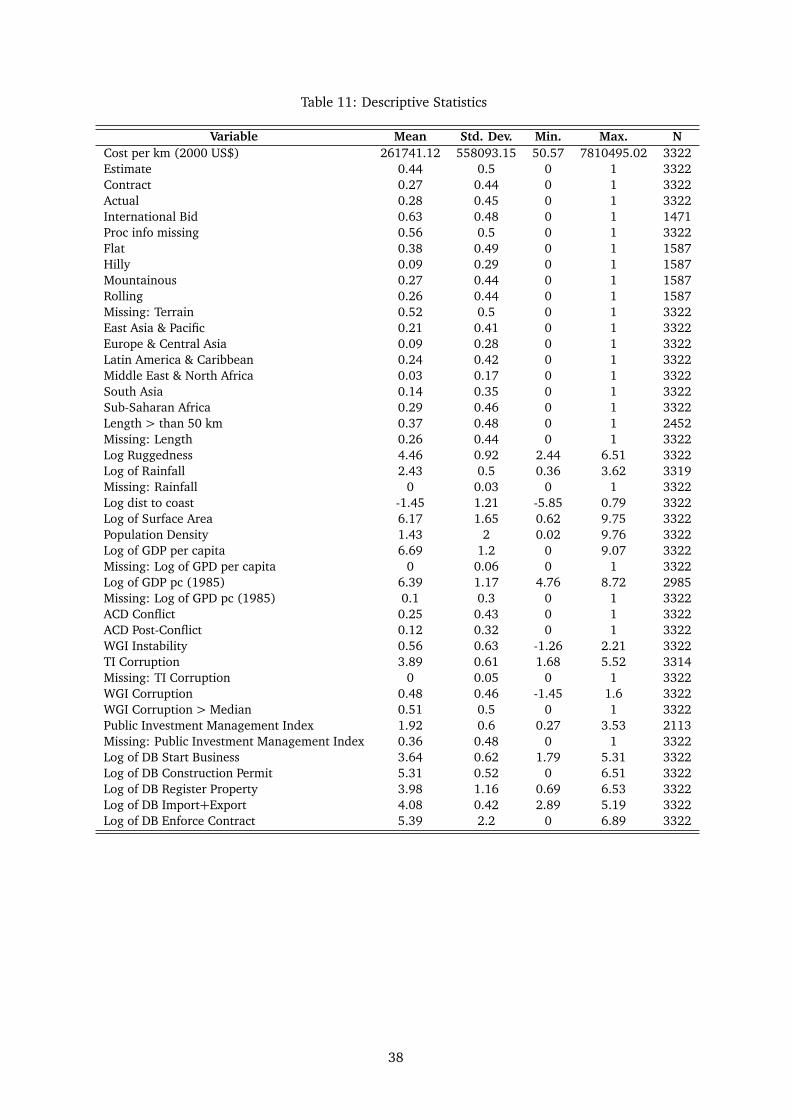
Table 11: Descriptive Statistics
Variable Mean Std. Dev. Min. Max. NCost per km (2000 US$) 261741.12 558093.15 50.57 7810495.02 3322Estimate 0.44 0.5 0 1 3322Contract 0.27 0.44 0 1 3322Actual 0.28 0.45 0 1 3322International Bid 0.63 0.48 0 1 1471Proc info missing 0.56 0.5 0 1 3322Flat 0.38 0.49 0 1 1587Hilly 0.09 0.29 0 1 1587Mountainous 0.27 0.44 0 1 1587Rolling 0.26 0.44 0 1 1587Missing: Terrain 0.52 0.5 0 1 3322East Asia & Pacific 0.21 0.41 0 1 3322Europe & Central Asia 0.09 0.28 0 1 3322Latin America & Caribbean 0.24 0.42 0 1 3322Middle East & North Africa 0.03 0.17 0 1 3322South Asia 0.14 0.35 0 1 3322Sub-Saharan Africa 0.29 0.46 0 1 3322Length > than 50 km 0.37 0.48 0 1 2452Missing: Length 0.26 0.44 0 1 3322Log Ruggedness 4.46 0.92 2.44 6.51 3322Log of Rainfall 2.43 0.5 0.36 3.62 3319Missing: Rainfall 0 0.03 0 1 3322Log dist to coast -1.45 1.21 -5.85 0.79 3322Log of Surface Area 6.17 1.65 0.62 9.75 3322Population Density 1.43 2 0.02 9.76 3322Log of GDP per capita 6.69 1.2 0 9.07 3322Missing: Log of GPD per capita 0 0.06 0 1 3322Log of GDP pc (1985) 6.39 1.17 4.76 8.72 2985Missing: Log of GPD pc (1985) 0.1 0.3 0 1 3322ACD Conflict 0.25 0.43 0 1 3322ACD Post-Conflict 0.12 0.32 0 1 3322WGI Instability 0.56 0.63 -1.26 2.21 3322TI Corruption 3.89 0.61 1.68 5.52 3314Missing: TI Corruption 0 0.05 0 1 3322WGI Corruption 0.48 0.46 -1.45 1.6 3322WGI Corruption > Median 0.51 0.5 0 1 3322Public Investment Management Index 1.92 0.6 0.27 3.53 2113Missing: Public Investment Management Index 0.36 0.48 0 1 3322Log of DB Start Business 3.64 0.62 1.79 5.31 3322Log of DB Construction Permit 5.31 0.52 0 6.51 3322Log of DB Register Property 3.98 1.16 0.69 6.53 3322Log of DB Import+Export 4.08 0.42 2.89 5.19 3322Log of DB Enforce Contract 5.39 2.2 0 6.89 3322
38

8.2 Tables and Figures
Table 12: Preservation Works
Work Class Work Type Predominant Work Activity
Routine Routine Maintenance Routine Maintenance Earth RoadRoutine Maintenance Gravel Road
Routine Maintenance Block 2L HighwayRoutine Maintenance Bituminous 2L HighwayRoutine Maintenance Concrete 2L Highway
Routine Maintenance Bituminous > 2L HighwayRoutine Maintenance Concrete > 2L HighwayRoutine Maintenance Bituminous ExpresswayRoutine Maintenance Concrete Expressway
Periodic Grading Light GradingHeavy Grading
Gravel Resurfacing Regravelling
Concrete Pavement Preventive Treatment Concrete Pavement Preventive Treatment
Bituminous Pavement Preventive Treatment Fog SealRejuvenation
Unsealed Preventive Treatment Unsealed Preventive Treatment
Surface Treatment Resurfacing Slurry Seal or Cape SealSingle Surface TreatmentDouble Surface TreatmentTriple Surface Treatment
Asphalt Mix Resurfacing Asphalt Overlay < 40 mmAsphalt Overlay 40 to 59 mm
Rehabilitation Strengthening Asphalt Overlay 60 to 79 mmAsphalt Overlay 80 to 99 mm
Asphalt Overlay > 99 mmMill and Replace
Bonded Concrete OverlayUnbounded Concrete Overlay
Concrete Pavement Restoration Concrete Slab ReplacementConcrete Slab Repair
Concrete Diamond Grinding
Reconstruction Reconstruction EarthReconstruction GravelReconstruction Block
Reconstruction BituminousReconstruction Concrete
39

Table 13: Development Works
Work Class Work Type Predominant Work Activity
Improvement Partial Widening Partial Widening to Gravel 2LPartial Widening to Block 2L
Partial Widening to Bituminous 2LPartial Widening to Concrete 2L
Partial Widening and Reconstruction Partial Widening and Reconstruction to Gravel 2LPartial Widening and Reconstruction to Block 2L
Partial Widening and Reconstruction to Bituminous 2LPartial Widening and Reconstruction to Concrete 2L
Widening Widening Adding Bituminous 1LWidening Adding Bituminous 2LWidening Adding Bituminous 4LWidening Adding Concrete 1LWidening Adding Concrete 2LWidening Adding Concrete 4L
Widening and Reconstruction Widening and Reconstruction Adding Bituminous 1LWidening and Reconstruction Adding Bituminous 2LWidening and Reconstruction Adding Bituminous 4LWidening and Reconstruction Adding Concrete 1LWidening and Reconstruction Adding Concrete 2LWidening and Reconstruction Adding Concrete 4L
Upgrading Upgrading to Earth 2LUpgrading to Gravel 2LUpgrading to Block 2L
Upgrading to Bituminous 2LUpgrading to Concrete 2L
New Construction New 1L Road New Earth 1L RoadNew Gravel 1L RoadNew Block 1L Road
New Bituminous 1L RoadNew Concrete 1L Road
New 2L Highway New Earth 2L HighwayNew Gravel 2L HighwayNew Block 2L Highway
New Bituminous 2L HighwayNew Concrete 2L Highway
New 4L Highway New Bituminous 4L HighwayNew Concrete 4L Highway
New 6L Highway New Bituminous 6L HighwayNew Concrete 6L Highway
New 4L Expressway New Bituminous 4L ExpresswayNew Concrete 4L Expressway
New 6L Expressway New Bituminous 6L ExpresswayNew Concrete 6L Expressway
40

Table 14: Cost per km for Different Work Types, by Work Category
Development
N mean p50 sd min maxNew 6L Expressway 1 5,571,488 5,571,488 . 5,571,488 5,571,488New 4L Expressway 65 2,838,562 2,495,592 1,474,420 937,499 7,810,495New 4L Highway 11 2,195,810 2,213,333 1,159,299 660,242 4,561,035New 6L Highway 2 1,990,155 1,990,155 991,449 1,289,094 2,691,215Widening and Reconstruction 108 874,209 776,071 752,950 178,494 6,532,523Widening 138 842,697 776,071 742,325 8,751 5,785,612New 2L Highway 68 750,396 696,537 399,828 22,403 1,985,876Partial Widening and Reconstruct 117 261,380 252,202 129,635 8,219 682,508Upgrading 360 250,472 218,863 171,322 3,551 940,837Partial Widening 12 137,773 148,321 29,027 67,299 168,278New 1L Road 7 91,788 81,244 36,153 58,151 167,702
Total 889 678,283 358,293 930,798 3,551 7,810,495
Preservation
N mean p50 sd min maxConcrete Pavement Restoration 4 539,348 650,623 321,650 68,558 787,587Reconstruction 745 220,287 169,668 209,577 1,973 2,615,657Strengthening 422 139,371 120,799 75,097 27,473 553,857Asphalt Mix Resurfacing 458 64,551 60,356 29,538 12,350 211,000Surface Treatment Resurfacing 230 25,090 18,767 23,520 3,409 176,682Gravel Resurfacing 275 18,169 13,198 15,765 1,872 112,950Bituminous Pavement PreventiveTreatment
47 7,355 5,534 6,190 1,147 30,653
Unsealed Preventive Treatment 101 4,347 4,385 1,319 2,009 8,402Routine Maintenance 119 2,144 1,897 1,383 277 8,685Grading 23 515 151 771 51 2,542
Total 2,424 109,930 67,561 149,738 51 2,615,657
41

Table 15: Cost per km for Development Works, by Work Activity
Development
work activity N mean p50 sd min max
New Bituminous 6L Expressway 1 5,571,488 5,571,488 . 5,571,488 5,571,488Widening Adding Bituminous 4L 2 4,643,333 4,643,333 1,615,426 3,501,055 5,785,612New Bituminous 4L Expressway 65 2,838,562 2,495,592 1,474,420 937,499 7,810,495New Concrete 4L Highway 1 2,213,333 2,213,333 . 2,213,333 2,213,333New Bituminous 4L Highway 10 2,194,058 2,177,899 1,221,993 660,242 4,561,035New Bituminous 6L Highway 2 1,990,155 1,990,155 991,449 1,289,094 2,691,215Adding Bituminous 4L 8 1,855,587 1,832,513 186,580 1,568,359 2,088,700Widening Adding Concrete 1L 2 1,641,940 1,641,940 21,358 1,626,837 1,657,043New Block 2L Highway 1 1,264,231 1,264,231 . 1,264,231 1,264,231Widening and ReconstructionAdding Bituminous 2L
61 1,085,967 989,080 790,232 241,875 6,532,523
New Bituminous 2L Highway 43 828,245 764,706 378,909 224,882 1,985,876Widening Adding Bituminous 2L 120 812,194 611,882 573,139 163,469 3,497,181Widening Adding Concrete 2L 2 626,842 626,842 163,489 511,238 742,446New Concrete 2L Highway 4 467,990 460,773 61,948 408,051 542,364Widening and ReconstructionAdding Bituminous 1L
36 304,665 257,007 126,310 178,494 616,324
Upgrading to Concrete 2L 13 302,035 356,189 149,254 55,523 465,583Upgrading to Bituminous 2L 283 276,508 241,148 166,059 29,897 940,837Partial Widening and Reconstruc-tion to Bituminous 2L
114 267,427 259,679 125,657 28,052 682,508
Widening Adding Bituminous 1L 7 265,241 260,115 287,751 8,751 702,651Upgrading to Block 2L 13 168,742 165,477 66,341 42,710 325,644Partial Widening to Bituminous 2L 12 137,773 148,321 29,027 67,299 168,278New Gravel 2L Highway 5 124,079 111,650 103,110 22,403 232,864New Gravel 1L Road 2 112,926 112,926 77,464 58,151 167,702New Bituminous 1L Road 1 99,800 99,800 . 99,800 99,800New Earth 1L Road 4 79,215 76,864 9,152 71,800 91,335Upgrading to Gravel 2L 32 58,825 52,491 32,724 15,940 161,949Partial Widening and Reconstruc-tion to Gravel 2L
3 31,614 13,288 36,219 8,219 73,334
Upgrading to Earth 2L 6 12,683 13,432 6,593 3,551 20,377
Total 853 682,288 348,307 947,126 3,551 7,810,495
42

Table 16: Cost per km for Preservation Works, by Work Activity
Preservation
work activity N mean p50 sd min max
Concrete Slab Replacement 3 696,277 684,879 86,177 616,367 787,587Reconstruction Bituminous 595 247,848 196,167 216,894 20,165 2,615,657Reconstruction Concrete 31 236,432 222,319 119,577 50,890 487,139Asphalt Overlay > 99 mm 91 183,925 167,059 76,022 56,275 478,158Asphalt Overlay 80 to 99 mm 140 136,484 118,752 70,626 38,583 553,857Mill and Replace 38 130,524 105,147 76,856 48,892 353,720Asphalt Overlay 60 to 79 mm 54 91,572 87,437 30,920 27,473 180,761Asphalt Overlay 40 to 59 mm 298 71,637 69,905 27,668 20,073 211,000Reconstruction Block 2 51,816 51,816 37,039 25,626 78,007Reconstruction Gravel 86 44,158 39,356 28,482 5,086 131,778Asphalt Overlay < 40 mm 81 41,963 38,078 17,396 12,350 95,148Double Surface Treatment 71 31,918 29,446 21,376 10,246 176,682Single Surface Treatment 61 21,431 18,254 14,773 5,295 106,457Double Surface Treatment 2 21,351 21,351 11,604 13,146 29,556Reconstruction Earth 7 20,834 17,724 17,029 1,973 56,561Regravelling 233 16,420 12,242 13,397 1,872 65,038Slurry Seal or Cape Seal 48 13,917 10,575 9,230 3,409 35,805Fog Seal 9 8,313 6,915 4,612 2,805 15,783Unsealed Preventive Treatment 99 4,277 4,343 1,236 2,009 8,402Routine Maintenance Block 2LHighway
2 2,728 2,728 1,736 1,500 3,956
Routine Maintenance Bituminous> 2L Highway
2 2,241 2,241 1,797 970 3,512
Routine Maintenance Bituminous2L Highway
71 2,232 1,964 1,232 332 5,580
Routine Maintenance Concrete 2LHighway
1 1,483 1,483 . 1,483 1,483
Routine Maintenance Earth Road 2 1,185 1,185 1,216 325 2,045Heavy Grading 9 1,144 591 948 323 2,542Routine Maintenance Gravel Road 17 1,110 1,229 616 277 2,042Light Grading 14 111 110 47 51 205
Total 2,067 116,228 71,896 156,977 51 2,615,657
43

Table 17: List of Countries (1)
1984-1990 1991-1995 1995-2000 2001-2005 2005-2008 Total
Afghanistan 0 0 0 12 0 12Albania 0 5 31 20 3 59Algeria 0 3 3 0 0 6Angola 0 0 0 8 0 8Argentina 0 64 17 15 19 115Armenia 0 3 48 0 0 51Azerbaijan 0 0 0 2 0 2Bangladesh 0 49 110 29 0 188Belize 0 0 0 3 0 3Benin 0 0 0 2 0 2Bhutan 0 0 0 4 3 7Bolivia 2 4 20 11 0 37Bosnia and Herzegovin 0 0 0 1 7 8Botswana 0 1 0 0 4 5Brazil 8 42 33 32 33 148Bulgaria 0 0 0 0 6 6Burkina Faso 0 0 0 24 2 26Burundi 0 0 0 3 2 5Cambodia 0 0 0 11 4 15Cameroon 0 4 12 13 0 29Cape Verde 0 7 0 8 0 15Chad 0 2 0 3 0 5Chile 9 12 11 0 7 39China 1 25 37 61 5 129Colombia 0 13 0 0 0 13Comoros 0 0 2 0 0 2Congo 0 0 0 0 1 1Costa Rica 0 0 6 0 0 6Dem. Rep. Congo 0 0 0 16 1 17Djibouti 0 0 5 6 0 11Dominican Republic 1 4 36 2 0 43Ecuador 0 1 0 12 0 13El Salvador 0 0 4 0 0 4Ethiopia 0 0 38 33 3 74Fiji 0 0 1 0 0 1Georgia 0 0 0 3 3 6Ghana 2 29 217 38 1 287Guatemala 0 3 0 0 0 3Guinea 0 1 0 9 0 10Haiti 0 0 1 7 0 8Honduras 0 12 6 0 14 32India 13 7 84 63 11 178Indonesia 0 9 8 21 1 39Iran 0 0 0 0 1 1Jamaica 0 1 0 0 0 1Jordan 0 4 4 0 0 8Kazakhstan 0 0 17 7 0 24Kenya 0 1 0 34 6 41Kyrgyz Republic 0 2 5 7 0 14Lao PDR 3 10 35 46 6 100
44

Table 18: List of Countries (cont.)
1984-1990 1991-1995 1995-2000 2001-2005 2005-2008 Total
Latvia 0 0 6 0 0 6Lebanon 0 14 9 25 0 48Lesotho 0 0 4 3 0 7Lithuania 0 0 5 0 0 5Macedonia 0 0 2 13 3 18Madagascar 0 1 1 8 0 10Malawi 0 3 0 15 0 18Malaysia 0 1 0 0 0 1Mali 0 2 3 2 1 8Mauritania 0 0 0 1 0 1Mauritius 0 2 0 0 0 2Mexico 3 8 49 2 0 62Moldova 0 0 0 0 2 2Mongolia 0 0 1 7 0 8Morocco 0 2 0 2 0 4Mozambique 0 0 0 21 3 24Namibia 0 0 0 3 0 3Nepal 0 8 7 7 7 29Nicaragua 0 8 11 20 0 39Niger 0 0 3 6 1 10Nigeria 0 11 22 11 9 53Pakistan 0 0 22 34 0 56Panama 0 0 12 33 0 45Papua New Guinea 0 4 1 29 0 34Paraguay 0 5 5 13 0 23Peru 0 14 8 5 0 27Philippines 5 26 61 52 10 154Romania 0 0 1 3 0 4Russia 0 44 17 0 0 61Rwanda 0 0 0 1 5 6Samoa 0 0 1 0 0 1Senegal 0 0 3 14 0 17Serbia 0 1 0 0 0 1Sierra Leone 0 6 0 7 0 13South Africa 0 0 0 3 0 3Sri Lanka 0 0 4 0 0 4Swaziland 0 0 0 1 0 1Tanzania 0 2 25 8 1 36Thailand 0 29 116 25 0 170Tunisia 0 6 2 4 0 12Turkey 0 0 2 24 0 26Uganda 0 11 173 18 0 202Uruguay 0 11 61 0 0 72Venezuela 0 1 47 1 0 49Vietnam 0 3 14 18 7 42West Bank and Gaza 0 0 3 0 0 3Yemen 1 4 3 2 0 10Zambia 0 16 0 15 0 31Zimbabwe 0 4 0 0 0 4
Total 48 565 1,495 1,022 192 3,322
45
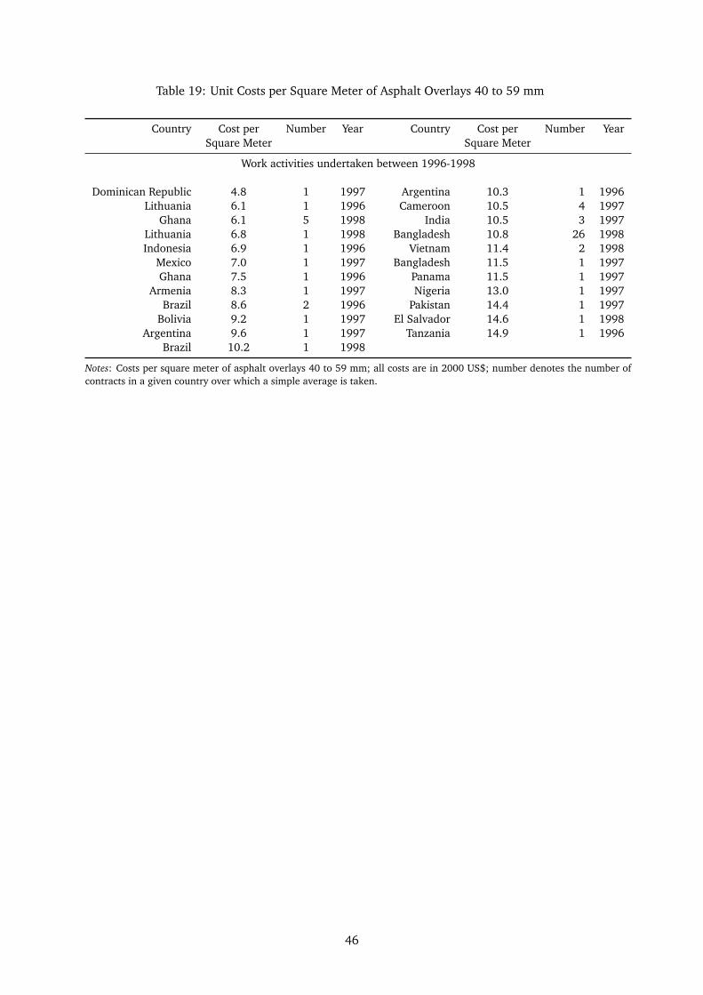
Table 19: Unit Costs per Square Meter of Asphalt Overlays 40 to 59 mm
Country Cost per Number Year Country Cost per Number YearSquare Meter Square Meter
Work activities undertaken between 1996-1998
Dominican Republic 4.8 1 1997 Argentina 10.3 1 1996Lithuania 6.1 1 1996 Cameroon 10.5 4 1997
Ghana 6.1 5 1998 India 10.5 3 1997Lithuania 6.8 1 1998 Bangladesh 10.8 26 1998Indonesia 6.9 1 1996 Vietnam 11.4 2 1998
Mexico 7.0 1 1997 Bangladesh 11.5 1 1997Ghana 7.5 1 1996 Panama 11.5 1 1997
Armenia 8.3 1 1997 Nigeria 13.0 1 1997Brazil 8.6 2 1996 Pakistan 14.4 1 1997
Bolivia 9.2 1 1997 El Salvador 14.6 1 1998Argentina 9.6 1 1997 Tanzania 14.9 1 1996
Brazil 10.2 1 1998
Notes: Costs per square meter of asphalt overlays 40 to 59 mm; all costs are in 2000 US$; number denotes the number ofcontracts in a given country over which a simple average is taken.
46

Table 20: Differences in Unit Costs across different Work Types
eq1 eq2(1) (2)
Preservation Works
Routine Maintenance -4.289∗∗∗ -4.256∗∗∗(0.143) (0.174)
Grading -6.396∗∗∗ -6.305∗∗∗(0.352) (0.374)
Gravel Resurfacing -2.275∗∗∗ -2.207∗∗∗(0.117) (0.159)
Bituminous Pavement Preventive Treatment -3.076∗∗∗ -2.989∗∗∗(0.134) (0.18)
Unsealed Preventive Treatment -3.375∗∗∗ -3.441∗∗∗(0.179) (0.193)
Surface Treatment Resurfacing -1.981∗∗∗ -1.917∗∗∗(0.135) (0.185)
Asphalt Mix Resurfacing -.848∗∗∗ -.862∗∗∗(0.092) (0.143)
Strengthening -.117 -.174(0.085) (0.15)
Concrete Pavement Restoration 1.000 1.045∗(0.629) (0.553)
Reconstruction 0.073 0.029(0.102) (0.157)
Development Works
Partial Widening and Reconstruction 0.258 0.405∗∗∗(0.224) (0.151)
Widening 1.410∗∗∗ 1.415∗∗∗(0.171) (0.21)
Widening and Reconstruction 1.539∗∗∗ 1.485∗∗∗(0.142) (0.188)
Upgrading 0.271∗∗ 0.229(0.118) (0.162)
New 1L Road -.349∗∗ -.027(0.148) (0.191)
New 2L Highway 1.529∗∗∗ 1.450∗∗∗(0.199) (0.245)
New 2L Highway 1.529∗∗∗ 1.450∗∗∗(0.199) (0.245)
New 4L Highway 2.542∗∗∗ 2.502∗∗∗(0.297) (0.305)
New 6L Highway 2.464∗∗∗ 2.405∗∗∗(0.097) (0.162)
New 4L Expressway 2.824∗∗∗ 2.735∗∗∗(0.072) (0.156)
New 6L Expressway 3.682∗∗∗ 3.406∗∗∗(0.127) (0.224)
Obs. 3322 3322R2 0.83 0.841
Notes: Omitted category is partial widening; column (1) includes year dummies and contract characteristics included inall models; column (2) also includes country characteristics; standard errors brackets, clustered at the country level; ∗,∗∗, ∗∗∗ denote significance at 10%, 5% and 1% levels.
47

Table 21: Baseline Results
BASEI BASEII BASEIII(1) (2) (3)
Estimate -.024 -.022 -.020(0.059) (0.058) (0.058)
Contract -.080 -.085 -.078(0.054) (0.055) (0.054)
Geography
Log Ruggedness 0.155∗∗∗ 0.151∗∗∗ 0.157∗∗∗(0.035) (0.037) (0.036)
Log of Rainfall -.028 -.041 -.036(0.07) (0.071) (0.071)
Log dist to coast -.023 -.040 -.020(0.051) (0.054) (0.051)
Population Density 0.105∗∗∗ 0.103∗∗∗ 0.107∗∗∗(0.019) (0.02) (0.02)
Log of Surface Area 0.081∗∗∗ 0.092∗∗∗ 0.081∗∗∗(0.022) (0.024) (0.022)
Length > than 50 km -.093∗∗ -.105∗∗∗ -.096∗∗(0.038) (0.039) (0.039)
Log of GDP per capita -.056(0.038)
Log of GDP pc (1985) -.005(0.046)
Pilot Country -.095 -.096 -.099(0.074) (0.079) (0.075)
East Asia & Pacific -.490∗∗∗ -.449∗∗∗ -.486∗∗∗(0.096) (0.107) (0.103)
Europe & Central Asia -.133 -.060 -.076(0.09) (0.103) (0.105)
Latin America & Caribbean -.175∗ -.066 -.167(0.098) (0.127) (0.141)
Middle East & North Africa -.438∗∗∗ -.340∗∗ -.372∗∗∗(0.106) (0.141) (0.113)
South Asia -.445∗∗∗ -.431∗∗∗ -.455∗∗∗(0.114) (0.121) (0.115)
Obs. 3322 3322 3322R2 0.896 0.896 0.896
Notes: Dependent variable is the log of cost per km; all models control for work activity fixed effects, year fixed effects,an interaction between work type and 5-year period fixed effects; base categories are actual costs; robust standard errorsin parentheses, clustered at the country; ∗, ∗∗, ∗∗∗ denote significance at 10%, 5% and 1% levels.
48