The Agglomeration of Headquarters∗

James C. Davis and J. Vernon Henderson

January 9, 2004

Abstract

This paper uses a micro data set on auxiliary establishments from 1977 to1997 in order to investigate the determinants of headquarter agglomerations andthe underlying economic base of many larger metro areas. The significance ofheadquarters in large urban settings is their ability to facilitate the spatial sepa-ration of their white collar activities from remote production plants. The resultsshow that separation benefits headquarters in two main ways: the availability ofdifferentiated local service input suppliers and the scale of other headquarter ac-tivity nearby. A wide diversity of local service options allows the headquarters tobetter match their various needs with specific experts producing service inputsfrom whom they learn, which improves their productivity. Headquarters alsobenefit from other headquarter neighbors, although such marginal scale benefitsseem to diminish as local scale rises.

∗The authors are respectively at the U.S. Bureau of the Census (jdavis@nber.org) and BrownUniversity (Vernon_Henderson@brown.edu). Henderson is the corresponding author. Support for thisresearch from NSF (award no. 0111803) is gratefully acknowledged. The research in this paper wasconducted while the authors were Census Bureau research associates at the Boston Census ResearchData Center (BRDC). Research results and conclusions expressed are those of the authors and do notnecessarily indicate concurrence by the Bureau of the Census. This paper has been screened to insurethat no confidential data are revealed. The authors thank Gilles Duranton for helpful comments, aswell as participants in seminars at LSE, USC, Johns Hopkins, Chicago, the AEA and RSAI meetings,and the Federal Reserve Banks of NY, Kansas City and Chicago.

1

1 Overview

The executives who make decisions on how their firms will be organized often find itadvantageous to locate headquarter facilities away from production facilities, in differ-ent metro areas. Given that intra-firm communication becomes more cumbersome andexpensive with physical separation, why is separation beneficial?

There are two competing explanations. First headquarters choose to locate inmetropolitan areas comprised of a wide variety of business service suppliers. Head-quarters need information, advice, and services from specialists in law, advertising, andfinance. Acquiring such information and services involves repeated face-to-face inter-action and close spatial proximity between buyers and sellers. We know service firmsare disproportionately concentrated in larger cities, so headquarters locate in theseservice cities away from smaller production oriented cities, because they benefit fromthe variety of differentiated suppliers. The second explanation is that headquarterscluster together to exchange information among themselves and acquire informationabout market conditions. This exchange, whether it involves deliberate ”trades” or”spillovers”, informs headquarters about production, input and technology choices fortheir plants. For example Lovely, Rosenthal and Sharma (2002) find exporter head-quarter activity is more agglomerated than other headquarter activity because exportrelated information is difficult to acquire. These competing explanations have impli-cations for how we model cities in an urban system, how we model agglomerationeconomies, and how we think of the nature of outsourcing decisions.

These competing explanations are also at the heart of current investigations intothe nature of scale economies that lead economic activity to agglomerate into cities.The traditional model (Fujita and Ogawa (1982)) is one of information spillovers; andin urban systems modeling (Henderson (1974), Duranton and Puga (2001)) these exter-nalities are viewed as internal to the own industry, consistent with empirical evidencefor manufacturing (see Rosenthal and Strange (2003) for a review). Own industry scaleexternalities lead to urban specialization, where cities specialize to exploit own indus-try scale, relative to general urban diseconomies such as commuting and congestioncosts. So we observe textile, steel, auto, insurance, entertainment and so on type cities(Black and Henderson (2003)), among medium and small size metro areas.

What about large metro areas, which have more diverse, service oriented economicbases (Kolko (1999))? One literature follows the scale externality explanation. Somelarge metro areas like New York City are viewed as being specialized in headquartersactivity, where presumably headquarters experience own industry scale externalities.But, since headquarters purchase business and financial services, they draw, almostincidentally, these activities into large metro areas as well (Ginzberg (1977), Aksoyand Marshall (1992)). However the recent economic geography literature deriving

2

from Krugman (1991), has a somewhat different perspective on essentially the samephenomenon.

In the new economic geography literature, agglomeration externalities derive fromdiversity in local intermediate input service sectors (Abdel-Rahman and Fujita (1990)).In a Dixit-Stiglitz-Ethier (1982) framework, greater scale and hence diversity in localbusiness service inputs makes final local (headquarter) production more efficient. SoDuranton and Puga (2002) model "functional" specialization (see also Davis (2003)).Smaller cities are specialized in production activities, while headquarters co-locate withlarge scale business service activity because of the scale economies from diversity inintermediate inputs, in large metro areas and away from production.

The main objective of this paper is to distinguish and quantify these two typesof scale effects for headquarters’ activity, the role of own industry scale externalitiesversus the role of diversity scale externalities, and thus improve our understanding ofthe agglomeration forces governing certain larger metro areas. Do both scale effectsexist and, if so, how important are they? This is the first time that we know of thatan empirical scale externality paper has looked at a service activity, as opposed to justmanufacturing production. As such, one might anticipate results to be quite different.In manufacturing, external scale elasticities tend to be in the 0-.12 range (Rosenthal andStrange (2003)), so, at most, a 10% increase in local relevant scale increases efficiencyby 1.2%. Manufacturing is found in smaller cities. For headquarters to pay the muchhigher wage, input, and real estate rental costs in larger cities we might expect to seemuch greater scale effects.

Apart from learning more about the fundamentals of agglomeration, the existenceand magnitude of local scale externalities has implications also for local public policy.In urban systems models (Henderson (1988), Duranton and Puga (2001)), achievingefficient city size requires application of the Henry George Theorem. Land rents (or landtaxes from property) are used to subsidize and internalize externalities, in a competitiveurban system. Metro areas are heavily involved in such subsidization activity, with 9/11putting this issue up-front in Lower Manhattan. The magnitude of externalities willdetermine the appropriate extent of subsidies, and later in the paper we will interpretour results in this context.

Finally this paper suggests out-sourcing behavior is an important aspect of pro-duction organization today, as documented in Ono’s (2001) work. While clusteredheadquarters learn from each other and in-house many of their service activities, theability to locally out-source special service activities explains why large market centersspecialized in such activities are attractive locations. Some out-sourcing activities areobservable (e.g., legal, accounting services) while others such as financial can only beinferred.

3

Data on HeadquartersThe establishment data on headquarters are from the U.S. Census Bureau’s Eco-

nomic Census data set on Central Administrative Office and Auxiliary Establishments[CAO] covering the period 1977-97 in five-year intervals.1 An auxiliary is any estab-lishment of the company whose principal function is to manage, administer, service,or support the activities of other establishments of the company (Census(1996)). Thisincludes administration and management, R&D, computer data processing centers,communications, central warehouses and trucking.

What we focus on is something called central administrative units, which we iden-tify informally as headquarters [HQ]2. As Table 1 reveals these comprise 73% of allauxiliaries in 1997. These facilities produce services that are consumed by the oper-ating units and plants of their firms. Examples include strategic planning, business,financial and resource planning, as well as centralized ancillary administrative servicessuch as legal, accounting, and the like. Some of these services may be out-sourced,given out-sourcing is also a central function of HQ’s. Starting in 1997, the Census alsoidentifies a small percent of auxiliaries that specialize in legal, accounting, advertisingor personnel functions for their firms. Our focus is just on HQ’s.

Each HQ unit is assigned an SIC code that corresponds to the industry of theoperating units it services. We distinguish between manufacturing, retail, service andother categories since they do exhibit fundamental differences.3 Table 2 shows theindustrial composition breakdown of HQ’s in 1977 and 1997. Manufacturing andretail/wholesale are the major HQ sectors, together accounting for 65% of HQ’s in1997 and both grew about 20% in counts from 1977 to 1997. In this data overview,we show both establishment counts and employment numbers, though in estimationwe focus on counts as the underlying model will suggest. The employment picture ishowever also of interest for comparison with the overall economy. Manufacturing HQ’sare much larger in employment than other HQ’s, 143% larger than the average sizeof all non-manufacturing HQ’s in 1997. However the rapidly growing sector, as with

1Auxiliaries are surveyed as part of the Enterprise Statistics Program under Economic CensusSpecial Programs. Auxiliaries are identified by multi-establishment company in the prior year as partof the Report of Organization questionaire for the Company Organization Survey and all reportedauxiliaries are subsequently surveyed. This is a rarely used data set whose features we are still learningabout. Earlier studies that used this data are Lichtenberg and Siegel (1990) who researched the laboreffect of ownership change, and Siegel and Griliches (1992) who used the CAO to complete the viewof service and computer inputs to manufacturing plants so as to investigate the impact of outsourcingon total factor productivity.

2In some years (1982-1992, but not 1977 or 1997), about 70% of central administrative units aredesignated as actual headquarters. Since we can’t make the distinction consistently over time andmany who are not identified as headquarters simply didn’t fill out the questionnaire, we use the centraladministrative unit designation and call all of these headquarters for the remainder of the paper.

3The "other" category includes industries that were not in scope through the whole sample periodof 1977 through 1997, and was excluded in estimation so that HQ birth measures would not reflectchanges in the scope of the Economic Census over time.

4

the economy, is business services, as well as personal services in the ”rest”. Note thatfor 1977, finance, real estate, insurance, and communications were out of scope in thesample frame. By 1997 these plus business services account for 11% of HQ’s.

Like operating plants, HQ’s have high “birth” and “death” rates. In Table 3, thebirth rate every five years is about .6. A birth is a new HQ in a county as identified bya new company plant identifier appearing in the county. Within a county, moves by acompany HQ are not counted as births; but, for example, only .2% of surviving HQ’swithin counties from 1992-97 report a new location-plant identifier (PPN), although amuch higher 17.8% appear to have a new zip code. Auxiliaries (CAO’s) that switchfrom being a non-HQ to a HQ are also not counted as births (these would increase thenumber of births by 15% from 1992-97). However buy-outs (which change the companyidentifier) are. Buy-outs in 1992-1997 are about 5.8% of births, as inferred byHQ’s thathave a new company identifier (CFN), but the same plant-location identifier (PPN).Before 1987 we can’t distinguish since we don’t have PPN’s for those years. Deathsare a HQ company-plant identifier disappearing from a county.

Table 3 shows that about 50% of HQ’s die out each five-year period. Such a highdeath rate initially struck us as odd. HQ’s belong to mature firms. What appears tobe the case is that many of these larger firms have many HQ’s, one or two of whichare the main operational HQ which may be ”permanent.” Of the 1977 HQ’s, 15%remained in the sample through the last year of our data in 1997. Firms perform alot of experimentation with both location choices for other headquarters and a lot ofexperimentation with whether to have a fourth or fifth, or tenth HQ facility. The fixedfinancial cost of setting up an office is not that high. It is this experimentation, aswell as decisions of firms without a HQ as to where to locate their first HQ, whichgenerates the births in our data. That will allow us to identify the effects of changinglocal economic conditions on HQ profits.

The next issue is location ofHQ’s. In Table 4 we aggregate counties into four groupsby employment size rank. The groups are the top 10 largest employment counties, thenext 11-75, the remaining urban counties, and rural counties. From Table 4, the largest10 counties in 1997 have a .15 share of all national private employment and .21 shareof all HQ employment, or a relative quotient of HQ share to total employment shareof 1.38. Likewise, mid to large sized counties ranked 11-75 collectively have a .29share of national employment and .39 share of national HQ employment, a quotientof 1.35. HQ’s are found in greater numbers in the large centers relative to what onewould expect given total employment there. In contrast, the relative HQ quotientfor the remaining urban counties is .87 and for rural counties .33. HQ are clearlyunder-represented in rural counties and we focus on urban counties for the remainderof the paper. We find a similar pattern for major business services, with high relativeshare quotients of 1.43 and 1.29 for the top 10 and 11-75 groups respectively, and lowquotients for both smaller urban and rural counties. Service industry data are fromCounty Business Patterns and the Standard Statistical Establishment List (SSEL)

5

for 1977-1997, covering all private establishments in the U.S. This is in contrast tomanufacturing, shown in Table 4 to have greater representation in smaller urban andrural counties. HQ and business services tend to be co-located in central counties oflarger cities.

Though Table 4 shows HQ’s are a large county phenomenon, Figure 1 revealssubstantial urban specialization in HQ’s. The figure plots for all urban counties thelocation quotient, the ratio of the share of HQ establishments to the share of totalprivate establishments, against the log of the number of total establishments in thecounty. The wide variance in location quotients indicates concentration of HQ intocounties that specialize in HQ production.

Two points are worth mentioning. First, we did not find that HQ either are over-whelmingly concentrated into the very largest counties such as New York, L.A. or Cookcounty of Chicago, as can be seen in the right most portion of Figure 1, nor did we findthat HQ activity dominates the local economy in the largest metro areas as impliedby some earlier literature. For a sample of 10 central HQ counties of the largest 10CMSA, on average HQ employment in each is only 3.9% of its total employment in1997. HQ are an important part of the local economies of large cities, but the notionof these large metro areas as HQ cities above all else is not apparent. New York county(essentially Manhattan) offers an interesting example. While New York has 1.9% of allprivate U.S. employment and 3.0% of HQ employment in 1997, it has 5.3% of nationalcommercial banking, 25% of securities, 7.6% of investment holding companies, 15% ofadvertising, and 7.2% of legal services. New York appears more of a business servicecity than a HQ city per se. Comparing similarly sized industries, commercial andinvestment banking and securities industries are the same size nationally as the HQsector but they account for about 14% of NY county’s employment, as compared to 4%for HQ’s. Advertising, legal, and accounting are about 7% of New York’s employmentbase, even though nationally these industries collectively are about 20% smaller thanthe HQ sector. The second point worthy of note is that we did not find in the dataa substantial suburbanization trend for HQ. For eight of these large 10 central HQcounties of CMSA (L.A. and Phoenix are single county PMSA), their shares in relationto the rest of their own PMSA did fall 9% from 1977 to 1997, but this parallels a similarfall of 8% in total employment over the period. 4

Finally, we have asserted that a key function of HQ’s is out-sourcing, informationon which we use later to interpret coefficients. We have direct data on legal, accounting,and advertising out-sourcing. Out-sourcing for architecture, R&D, and the like are notrecorded. Second, out-sourcing in the financial sector is not ”observed”; it is buried in

4For this same sample of 10 central HQ counties, their share of CMSA HQ’s does drop from 69to 60% from 1977 to 1997, but that seems part of a general decentralization movement where the top10 CMSA’s share of national CA’s falls from 33 to 30% and the share of the central PMSA in CMSACA’s for the top 10 declines from 81 to 74%.

6

loan costs and rates of return. Table 5a shows the propensity of HQ’s to out-source foreach of the three reported industries. We note that in 1997 about a third of HQ’s donot fill out detailed information on questionnaires, and our numbers are based on HQ’swho do respond to the questionnaires. Out-sourcing propensities for HQ’s in 1997 are55-65% each of accounting, legal, and advertising. Among those HQ who out-source,Table 5b shows their share of out-sourcing expenditures for each industry in the HQwage bill. These direct numbers suggest for these three inputs alone out-sourcing is65% of the wage bill. Of these three, it is clear advertising out-sourcing is an importantfunction of HQ’s. These advertising expenditures are presumably billings and reflect ahigh proportion of money going for air time and ad space in the media, as opposed tojust compensation paid to advertising agencies per se. On the other hand they don’treflect company advertising decided by headquarters, but assigned as billing expenseshandled by other units of the company once an advertising campaign is underway.

In the paper we will be thinking of a model in which for certain cities, HQ’s are araison d’ betre. But we note that the very largest metro areas like New York may notembody this idea. The idea may be more applicable to metro areas like Charlottesville,VA, Milwaukee, WI, Rapid City, SD, and New Brunswick, NJ, examples with largelocation quotients (see Figure 1).

2 Modeling Headquarters’ Location

We now turn to modeling headquarters’ activities, with the intent of deriving a profitfunction for such activities. With a profit function, we can assess the role and im-portance of local wages, service offerings, and HQ agglomeration in the technology ofproducing headquarters’ activities. Of course headquarter profits are not observed perse. But we will take the model structure and use it to examine patterns of births ofHQ’s. From that we will determine the relative effect on inferred profits of differentattributes of counties, in terms of relative wage, service offerings, and local agglomer-ation.

Headquarters Technology.We assume headquarters produce service outputs Y consumed by their within firm

production plants. The HQ production function is given by

Y = A(HQ, .)Lα11

mQj=2

µnjPi=1

Xρjji

¶αjρj

(1)

Headquarters face costs

C = wL1 +mPj=2

njPi=1

qji Xji (2)

where A(HQ, .) is the level of technology in HQ production and L1 is headquarterlabor. A(·) will be specified to be a function of the number of other local headquarter

7

facilities nearby, under the assumption that this measure of the count of sources oflocal information spillovers represents the degree of local scale externalities, as willbe consistent with the econometric results. The subscript j represents the (m − 1)separate service industries. Xji is the purchase by a headquarter from firm i in serviceindustry j, where nj is the number of sellers in the local market in service industry j.qji is the price charged by firm i in industry j. We will generally work with 10 differentinput service industries. The parameter ρj is the technological need for variety ofdifferentiated service inputs from industry j in headquarters production, and the αj’sare share parameters. 0 < ρj < 1. The closer ρj is to one the more substitutable areinputs from industry j and the less important diversity is to headquarter’s production.Note σ = 1/(1− ρ), where σ is the elasticity of substitution.

With the symmetry that will result in equilibrium, the production function can berewritten

Y = A(HQ, .)Lα11

mQj=2

µn

αjρj

j Xαjj

¶(3)

Because each service is differentiated, nj gives the variety of service offerings in industryj available to the HQ locally. Differentiated service inputs bought by headquarters areassumed local to each city due to the need for face-to-face interaction during servicepurchase and delivery. Increased varieties offer a better match between service offeringsand HQ need, increasing efficiency as specified in the technology of the productionfunction as shown in (3). Note other things being equal, in this Dixit-Stiglitz varieties

formulation, HQ’s would prefer more varieties (nαjρj

j ) as opposed to more of any onevariety (Xαj

j where αj <αjρj). However the cost structure in Xj production limits the

number of varieties.

Each service provider belongs to only one industry, and firms within each industryface local monopolistic competition among each other. The labor Lji required by adifferentiated service firm to produce total local output X̃ji is

Lji = fj + cjX̃ji (4)

Firms within each industry are assumed identical local monopolistic competitors facingincreasing returns. Service production processes include a fixed cost of labor fj anda constant marginal cost cj. The local cost of labor to producers in the industry iswj. Note all local providers in industry j face identical technology, demand, and costs.Solving the symmetric equilibrium5 for each industry gives local prices of

qj =wjcjρj

(5)

5See Dixit and Stiglitz(1977), Abdel-Raman and Fujita(1990) or Davis(2000) for more details.

8

for service industry X̃j. As usual, ρj indicates the extent of the price markup by themonopolistic competitor.

Headquarters maximize profits where, from (1) and (2), profits are pY − C. p isthe unobserved (shadow) price, or unit value of an headquarter’s activities to the firm.That would depend for example on the unobserved distances in this data set from theheadquarter to the various plants or establishments of the firm. The fact that neither pnor Y are observed raises econometric issues for analysis below. Keeping this in mind,maximizing headquarter profits, with the assumption of symmetry among service inputsuppliers within each industry, the problem6 reduces to satisfying

L1 =pα1Y

wXj =

pαjY

njqj(6)

The next step is to define the profit function for headquarter’s activity. Givenprofits are pY − C; by substituting (5) and (6) into (2), we can show profits are pY(1 − α1 −

Pj

αj). Existence of a profit function requires (1 − α1 −Pj

αj) > 0, so we

can define α as the “owner’s” residual share where

α ≡ (1− α1 −mPj=2

αj) (7)

By substituting (4) and (5) into (1) we can solve for Y and then for profits. The resultis

π̃ = Bp1α A(·) 1α I−

1αw−α1/α (8)

where B is a parameter collection7 and I is a “price” index for differentiated products.I is given by

I =mQj=2

Ãwj

n(1−ρj)/ρjj

!αj

(9)

The index, I, plays a critical role in birth analysis below and its measurement will bediscussed. What this paper will attempt to sort out is the roles played by availabilityof service input varieties versus local scale externalities within the headquarter’s sectorin attracting headquarters to a city, in the profit function in (8).

Headquarters Agglomeration in a Systems of Cities Model.In a systems of cities model, one type of city would be headquarter cities (Davis(2003)).

For those types of cities the traded good output is headquarters’ activity, and interme-diate inputs are local business and financial services. In the standard city developer

6The first order conditions are ∂π∂L =

pα1YL − w = 0, ∂π

∂Xji=

pαjY

X1−ρjji

PXρjji

− qji = 0.

7B = α ααj/α1

mYj = 2

(αj ρj/cj)αj/α.

9

model (Henderson (1988), Duranton and Puga (2001)), one can set up the developer’soptimization problem. For that, the literature has internal space to cities and com-muting costs, where workers live on lots of fixed size in a circular city and commuteto work at the city center. Standard results yield total urban land rents of 1

3π−12 tN

32

where t is the cost of commuting a unit distance and N is city population and workforce.

The developer’s optimization problem is to maximize

1

3π−12 tN

32 − τ 1n− τ 2HQ− τ 3N (10)

which is total urban land rents collected minus subsidies to intermediate producers (τ 1)where there is just one type of intermediate input with share α2 for purposes of illustration,subsidies to each HQ (τ 2), and any subsidies to workers (τ 3). The developer faces twoconstraints. First, HQ’s must earn the going profit rate in national markets (πo),where per headquarter profits in equilibrium are revenue (HQεLα1

1 nα2ρ Xα2) less costs

(wL1 and qnX) plus subsidies (τ 2). Second, workers must earn the going real incomein national markets (I), where their income in the city is w − π

−12 tN

12 + τ 3, where

the middle term is per person rent plus commuting costs. In setting up the problem,two assumptions are made (consistent with a first best). First, wages w in the city arethe marginal product of labor in the HQ sector. Second, for intermediate producers,profits are zero where profits are revenue (qX̃) minus wage costs wL plus subsidies τ 1where L = f + cX̃.

If we do this optimization problem, with respect to τ 1, τ 2, τ 3, n, L, L1, HQ, andN (where N = nL+HQ L1), we can show the following standard results of relevancehere:

τ 2 = εHQεLα11 n

α2ρ Xα2 = εY

τ 1 = fw and τ 1n =α2(1−ρ)

ρ(HQ Y )

τ 3 = 0

(11)

The first term says, as always with externalities, that the subsidy equals the externalbenefit of an additional HQ: the spillover elasticity times the value of output. Thesecond term says, under monopolistic competition, firms should be paid their fixedcosts. But the real issue is the extent (n) of these fixed cost subsidies. Equation (11)tells us the total bill (τ 1n) is

α2(1−ρ)ρ

of total headquarter’s output. It is increasingas ρ declines and inputs become less substitutable. τ 3 = 0 because labor imposes noproduction externalities, in this formulation. These results will be used to give a publicpolicy interpretation to econometric estimates later in the paper.

3 Headquarters’ Location Choice

To model headquarters’ location, we assume firms (whose other activities we don’tobserve in the CAO data set) look nationally and choose profit maximizing locations

10

for their headquarters. We focus on the location of births - new (and relocating) HQ’sof firms. Patterns of where firms locate new HQ’s change over time, as economicconditions in different locations change over time. These conditions change, in largepart exogenously to HQ’s, in response to local shocks affecting the local service sector,amenities for consumers making migration decisions, and the local labor market asaffected by other economic sectors. As relevant local economic conditions change, thecomparative advantage of different locations for HQ’s changes. We look at the impactof changing economic conditions on the location patterns of births, since births canreadily respond to these changes. This will allow us to identify the effects of changingcovariates in equation (8) on implied profits.

An alternative would be to look at the location of stocks, or of net changes in stocks.Stocks include some long termHQ’s of firms where relocation costs would be very high,due to accumulated social and within firm human capital at a location. Net changesare composed of births and deaths. Other work on location (e.g., Davis, Haltiwangerand Schuh (1992), and Becker and Henderson (2000)) indicates the birth and deathprocesses do not mirror each other, with deaths being largely due to idiosyncraticfactors. Also there are switches where an auxiliary becomes an headquarter or nolonger primarily performs headquarter functions. For these types of reasons, mostauthors focus on births, dating back to Carleton (1983).

To analyze location decisions for births, we conceptualize in a discrete logit frame-work (Goldberg (1995)), where firms look across locations to pick the profit maximizinglocation for their new HQ’s. That is, given the total number of HQ’s born in time t,firm i chooses location k if from equation (8)

ln eπikt + fk + εikt > ln eπijt + fj + εijt ∀j (12)

where we define

πikt ≡ ln eπikt = lnB + 1

αln pikt +

1

αlnAkt(.)−

1

αln Ikt −

α1αlnwkt (13)

In the CAO data set, we have no characteristics of firms per se and no comprehensivecoverage of characteristics of HQ’s other than their industry and location.8 Nor dolocation attributes vary within a location by individual HQ. Thus we have a standardconditional logit, where the only variation is from locational characteristics, not firmones. Second, in (13) we do not observe the shadow price pikt for firm i. That effect,after controlling for county market potential and/or scale or CMSA scale, then issubsumed in the error structure in (12), for the draw on the "match," εikt, for how wellfirm i matches to location k, based on the various locations of its production or salesfacilities in relation to k. The εikt are i.i.d. and for the moment we assume they areWeibull distributed. The "fixed effect," fk, refer to unobserved time invariant locationcharacteristics.

8This follows from a 35-40% non-response rate to characteristics questions in the CAO.

11

If the covariates in (13) are exogenous to contemporaneous shocks, then we couldestimate the model by standard conditional logit methods, introducing regional "fixed"effects, or location dummies. However as Guimareaes, Figueiredo andWoodward (2000)show, in a Poisson model where the probability of observing βkt births in location k intime t is

prob(βkt) =e−λktλ

βktkt

βkt!, (14)

if λj is parameterized asλkt = exp(πkt + fk) , (15)

then the problem may be equivalently estimated by a "fixed effects" Poisson, eitheradding locational dummies to an ordinary Poisson or conditioning out location dum-mies by modelling the sequence of births for a location over time, conditioned on totalbirths over time for that location (see Hausman, Hall and Griliches (1984), as well asWooldridge (1991), and Papke (1991) and Becker and Henderson (2000) for applica-tions).

We will present ordinary Poisson and fixed effect Poisson results with standarderrors robust to the Poisson assumption, where the coefficients are computationallyidentical to respectively ordinary conditional logit and ordinary conditional logit withlocation dummies. The approach is flexible, with the logit-Poisson equivalence holdingwith time dummies, and industry groupings (e.g. manufacturing, service and retailHQ’s). Note that conceptually we are using either a discrete choice or discrete countmodel, rather than a continuous, or share specification (Berry (1994)) because of thenature of the dependent variable. Over half of our period-location observations willinvolve 5 births or less.

In estimation of the parameters of (13), births in time t are new HQ’s that appearbetween t and t + 1, where periods are spaced five years apart. A birth is a HQ in alocation that is present in t+1 but was not present in t. Births that occur after t but diebelow t+1 are not observed. πkt is a function of base period, t, location characteristics.So we are looking at the location decisions of waves ofHQ births. Identification is based(see next) on how the spatial patterns of births change in response to changes in localeconomic conditions. As formulated, firms base birth-location decisions in time t on thecounty characteristics in time t, which, strictly interpreted, implies naive expectationsin a dynamic model. We will comment more on this below.

Endogenous Covariates. In the ordinary and fixed effect Poisson we treat countycharacteristics such as prices and numbers of local business service providers as strictlyexogenous. However local industry scale measured by the number of headquarters inthe base period cannot be strictly exogenous. Contemporaneous errors which lead togreater births in t thus directly affect own industry scale in t which may be a covariatein t + 1 births. Thus it is desirable to instrument for own industry scale. In addi-tion treating own industry wages as exogenous is suspect. Similarly, aggregate county

12

shocks affecting headquarter births may reflect phenomena affecting all economic ac-tivity throughout the county.

Given expected births, λkt, actual births, βkt could be described by

βkt − λkt = ukt, λkt = exp (πkt + fk) (16)

where ukt is a contemporaneous error term. Covariates are predetermined and or-thogonal to uks, s ≥ t. To estimate the model with instrumental variables, we followChamberlain (1992) and Wooldridge (1997) (see also Windmeijer (2002) and Blun-dell, Griffith and Windmeijer (2000)); and we use a quasi-differenced transformationto eliminate the fixed effect, where

skt = βkt exp (πkt−1 − πkt)− βkt−1 (17)

Then the moment condition9

E£skt| zt−1k

¤= 0 (18)

is utilized in estimation. Thus this is a distribution-free version of the Poisson countmodel. zt−1k = (zkt−1, zkt−2, ...) are predetermined variables defined below. We stop attwo periods of predetermined variables in all period (differenced) equations, except forthe first period equation where we have only one period of predetermined variables.Estimation is by GMM (Hanson (1982), Windmeijer (2002)), with an efficient weightmatrix computed from first-step parameter estimates.

In instrumenting we will use generally past levels of covariates as instruments forcurrent changes (in the (πkt−1 − πkt) expression in (17)). The issue for the own scalevariable, HQ, in particular is why past levels are strong instruments. If all HQ’s wereperfectly mobile, then we would rely on mean reversion arguments. A high εkt−1 wouldresult in high HQkt. Then in t an expected lower εkt would result in a lower HQkt+1;then HQkt+1−HQkt < 0 and is negatively correlated with HQkt. But in estimating abirth model, we are clearly not assuming perfect mobility.

At the other extreme, we could assume compete immobility upon birth. Somedegree of immobility is dictated by physical HQ relocation costs, and by social re-location costs (costs of rebuilding a social network). But for purposes of illustra-tion, assume complete immobility. Second, assume more realistically that there isan "exogenous" death process where idiosyncratic firm level shocks that are not lo-cation specific put, on average, δ fraction of HQ’s out of business each period. Asnoted earlier this is motivated by the empirical work of Davis, Haltiwanger and Schuh

9Note skt = λkt−1 (ukt − ukt−1) .

13

(1992). These two assumptions imply a stock adjustment, or linear feedback, modelHQkt+1 = HQkt(1− δ) +B(HQkt,Xkt,εkt), where Xkt are covariates influencing profitsof births. Lets say the B(.) function has a form γoHQkt + γ1Xkt + εkt. Then invok-ing the model for periods t + 1 and t, and differencing we have HQkt+1 − HQkt =−δ(1− δ+ γo)HQkt−1− δγ1Xkt−1+ γoHQkt+ γ1Xkt+ εkt− δεkt−1.10 In practice HQkt

and elements of Xkt are not exogenous to εkt−1. But we can see that HQkt+1 −HQkt

is negatively correlated with both HQkt−1 and Xkt−1, where in our data δ ≈ 0.5.

We do not impose nor estimate a linear feedback model for two reasons. First isleakage, a high proportion of "switches," or auxiliary units of firms that change statusfrom non-HQ to HQ or vice versa, which we don’t count as births. Second, we expectsome dependence of δ on local economic conditions. However as long as there is areasonable degree of immobility, with δ largely dependent on firm idiosyncratic shocks,that are not location specific, then past levels of covariates will be strong instrumentsfor current changes.

In terms of specific details for variables such as HQt+1−HQt or Xt+1−Xt, we ex-perimented with instruments from t and t−1, as well as a more conservative approachwith instruments from t−1 and t−2. For all covariates except own industry wage (theα1/α coefficient in (13)), using the two approaches, results are almost identical. Firststage regressions of covariates (in changes) on level instruments all produce F ’s wellin excess of 10, and specification tests are strong. But under the more conservativeapproach, the own wage coefficient is much larger (in absolute terms). The concernwith downward bias in the more aggressive approach is the following. Consider 92-97births. A positive local own (HQ) sector shock in 1991 would not have time to sub-stantially affect 87-92 births and stocks, but could strongly affect 1992 wages as localHQ’s respond to the positive shock in the short-run by trying to hire more in the locallabor market specific to HQ workers. For covariates other than own industry oneswe instrument with t and t− 1 covariates but for own industry ones (own wages andHQ stock) we use t − 1 and t − 2 covariates.11 For own industry wages only, theselagged covariates are weak instruments; and we add lagged values for crime, federal em-ployment, and local government expenditures, which helps considerably. Governmentexpenditures provide positive amenities, and crime negative amenities. Workers mustbe compensated for increases in local crime if they are expected to continue to workin the county. Local changes in federal employment are both politically motivated aswell as decisions that are made in Washington, and the local crowding effect of theseexternal shocks linger through labor market adjustment.

10Note existence of long run stationary equilibrium where HQkt+1 = HQkt requires δ > γo.11One issue with this approach is for the earliest equation year, no HQ stock variable is available

for an instrument. The F -statistic for first stage regressions is nonetheless still above 10 using theremaining other instruments, indicating as a practical matter that instrumenting is sufficiently strongeven in the earliest equation year.

14

4 Empirical Implementation

In estimating eq. (13), we will distinguish separately births in three headquartersectors — manufacturing, retail, and services. These represent traditional larger (man-ufacturing) and smaller (retail) size headquarters along with a rapidly growing sector(services). Coefficients are constrained to be the same across groups, with separateeither time or sector-time dummy variables controlling for differential overall nationalsector growth. Identification comes from overtime variation in births within countiesfor each sector.

In addition to distinguishing three output/birth sectors, on the input side we po-tentially have ten sectors. Two are financial services — security and commodity brokers(6200) and holding offices (6700); and eight are business services — advertising (7310),employment agencies (7361), computer and data processing (7370), legal (8100), engi-neering and architectural (8710), accounting (8720), research and testing (8730) andmanagement and public relations (8740).12 To make the problem manageable, we makeseveral assumptions focused around the construction of the I index in eq. (9).

Service Index.Amajor focus of the paper is to sort out the importance of diversityof business service inputs, which in part comes down to estimating ρ’s for differentinputs. In our primary results, we will assume after some experimentation, that serviceinputs may be grouped into two categories, business and financial services each withtheir own ρ’s, each of which is assumed to be the same for all individual industrieswithin the category. In looking across the three headquarter sectors we assume thelabor share coefficient α1 and the sum of input share coefficients , αT , where

αT ≡11Pj=2

αj

are the same, which means α = 1−α1− αT is the same over time and sectors. However

we will allow the ratioαdjαTto differ by sector, d, manufacturing, retail and business

headquarters, and by year. The distinction allows for greater relative use of advertisingin, say, the retail versus manufacturing sectors, and that relative use to change overtime. We also experimented with allowing α1

αto vary for αT

αfixed, so αT can grow as

α1 declines, but found no evidence of consistent movements in αT .

For each output/birth sector in each year for each service input we calculateαdjαT

from input-output tables for the relevant input year. So for manufacturing in 1987,

for advertisingαdjtαTequals expenditures by all manufacturers on advertising divided by

expenditures by all manufacturers on all 10 service inputs. Then the I index in the

12Industry codings change over time. So 8710 is 8910 in earlier years and 8720 is 8930. SIC 8730 is7391 plus 8922 plus 7397 through 1987 and then 8731 plus 8733 plus 8734 beyond 1987. SIC 8740 is7392 through 1987 and then 8741 plus 8742 plus 8743 plus 8748 plus 8732 beyond.

15

profit function for business service inputs (IB) for sector d headquarters in location kin time t is

− 1αln IBd

kt = −³αT

α

´Pj B

αdjt

αTlnwjkt +

µαT

α

(1− ρB)

ρB

¶Pj B

αdjt

αTlnnjkt (19)

The coefficients to be estimated are in parentheses. A similar index IF is calculatedfor financial service inputs, where ρF differs from ρB. In estimation (a) the wage indexcoefficient αT

αin (19) should be the same for financial and business services (b) the own

industry wage coefficient (α1α) in equation (13) and the index wage coefficient in (19)

( α1αT) allow us to identify α1 and αT , and (c) the ratios of the n index coefficients to

the wage index coefficients identify (1−ρB)ρB

and (1−ρF )ρF

.

In estimation, we need observations on the ln wjkt and ln njkt variables for all 10input industries.13 Wages, wjkt, are median annual wages paid by establishments incounty k in industry j in time t (from the SSEL files of the Census for all private es-tablishments in the USA), where establishment wages are average wages per employee.The median is used to deal with the problem of outliers (small establishments witheither incredibly high (e.g. $300,000+) or incredibly low wages (e.g. $500)) in countieswith low njkt. Counts, njkt, are from County Business Patterns.14

Scale. Local scale of HQ’s inducing for example information spillovers, is measuredby a count of HQ’s in the own county in the base period, as opposed to total HQemployment based on empirical evidence below. For each HQ sector, based uponexperimentation, the scale variable is total HQ’s, including the own and other twosectors. We also allow for urbanization economies as represented by local county orPMSA employment and experiment with a variety of scale formulations.

Wages. Wages are average HQ wages in a county in a sector (manufacturing,services, retail) in the base period. That is they are average wages in existing HQ’sprior to these births. Such a measure does not capture the diversity of types of HQemployees and their relative costs, but it is the only measure widely available. We alsoexperiment with and get almost identical results using the median of the within HQwage average for a county.

Headquarters’ Price and Other Unobserved Prices.What internal price theHQ receives for its “output” is not observed. We hypothesize that the value of HQ

13The analysis is restricted to urban counties, since beyond urban counties most counties havemissing observations on wjkt or njkt for some j. Even with urban counties we must restrict thesample to birth counties in a year where all 10 wjkt and all 10 njkt have non-zero values. That losesabout 6% of urban county-year-sector observations.14Why don’t we use the SSEL for counts? The SSEL contains many irrelevant establishments that

are flagged (e.g. historical establishments out of business in the year of observation). Even aftereliminating flagged observation, SSEL counts don’t match CBP, who further clean the data to retainonly active establishments.

16

output to a firm increases with the size of the local or regional market and declines withdistance from the associated plants of the firm, also unobserved and captured in theunderlying matching error term between a location and facility. To capture market sizeeffects, we experimented with a measure of “market potential” of the county the HQchooses and also the size of the local metro area. Market potential in t is the sum acrossall counties of all private employment by county discounted by distances between thecentroid of the receiving county and the other counties. This sum in each year is thennormalized by the average sum for the year (so USA growth in employment over years isneutralized). Market potential (MP ) had no consistent effect on results. A variable wehaven’t discussed is office rent, which varies across and within metro areas. We don’thave office rent data by county. In estimation we experiment with some proxies, where,controlling for county employment (which reflects urbanization economies, market sizeeffects on value of headquarter activities to a firm, and congestion), rents might beexpected to rise with regional (CMSA) or metro (PMSA) overall size, negativelyaffecting profits.

5 Results

In presenting results, we start with our base set of results and then we turn to a detaileddiscussion of both scale effects and the geographic unit of analysis. The overall resultsare in Tables 6 and 7, where ordinary Poisson, county-sector fixed effect Poisson, andinstrumental variable GMM results on the non-linear model are presented. Our focuswill be on the GMM results, in Table 7.

Ordinary Poisson results in Table 6 are, predictably, unsatisfactory, with positive orweakly significant cost or wage index15 coefficients, indicating high cost areas are oneswith other unobserved good attributes. Fixed effect Poisson results start to take careof this problem by controlling for these attributes, giving significant own wage, and nindex and w index coefficients of expected sign. However, under fixed effects, strictexogeneity of the covariates will be violated for the stock of headquarters variable. Ownsector scale effects are of the wrong sign. In column (4) of Table 6 they are negative(mean reversion), and in column (5) insignificant, in strong contrast to GMM resultsin Table 7. Table 7 contains our key results and we now turn to them.

Service Diversity Effects.

We first look at the service input variables in column (1). From equation (19),the ratio of the n index to w index coefficients for business services equals (1−ρB)

ρB.

In Table 7, column (1), this implies a ρB of .49. Standard errors for this non-linear

15Recall that the business services wage index is constructed with wages in the service industries,so the wage paid to the lawyer is a cost to the HQ.

17

transformation of the coefficients are given in Table 8, which shows the estimate isstatistically significant. This ρB indicates a fairly low degree of substitutability amongbusiness service providers and a strong role for diversity. In terms of scale effects if thenumber of all business service providers increases 10%, the expected number of births(and profits) would rise by about 3.6%. That is a very large scale effect. Note wehave scaled the coefficient by .75 to reflect that business service inputs (αB) are onlya fraction of total service inputs (αT )16. If business service costs rise 10% as reflectedin the wage index, the expected number of births declines 3.5%.

For financial services the implied ρF =.51, similar to that for business services. Un-der GMM the financial services variables themselves are either insignificant or weaklysignificant in Table 7. However, the ratio defining ρF yields a ρF that is significant inTable 8. But financial services is potentially troublesome because we do not have veryprecise measures of the components of financial services where local diversity is impor-tant. For example, we dropped banking because we couldn’t break out componentsrelevant to businesses.

Own Sector Scale Effects.

Turning to own industry, or headquarter external scale economies, in Table 7 column(1), the scale elasticity is high, .17, and significant (Table 8). To get the elasticity (ε)of .17, we scale the coefficient (ε/α) by α=.56.17 Similar estimates for manufacturingproduction activities in the literature yield smaller estimates of, say, .03-.12. Column(2) suggests a non-linear form, where the scale variable is the inverse of the numberof HQ’s in the county. The elasticity starts high, at 3.5 for one headquarter and isever declining with larger HQ scale. At the mean number of 60 headquarters, theelasticity is .058, and for example at 133 HQ the elasticity is .026, and from Table 8the estimates are significant. Having a few other headquarters nearby to learn from isextremely beneficial, but as the number escalates those marginal benefits decline. Thisdeclining elasticity may explain the lack of very high concentrations of HQ’s in thelargest cities. Column (3) shows an alternative declining elasticity specification usinga quadratic term. Here the elasticity starts at .55 for one headquarter and also thendeclines. At the mean number of headquarters the elasticity is .086, and the elasticitypeters out to zero at 133 HQ in a county. However 11% of the counties in the samplehave HQ scale larger than 133. Also, in Table 8, the precision of estimates declinessharply as scale increases for this specification in which the elasticity declines to zero.

While own sector external scale effects are very large, the evidence that they declinesharply suggests that these scale effects alone cannot explain why some larger cities

16The rise is (1−ρB)ρB

αBα where αB is the sum of business service input coefficients. If αT

α = .45from the business w coefficient, we assign αB

α ≈ .35, as business services comprise the majority ofindustries in αT .17From equations (13) and (19), the sum of the coefficients for HQ wage and business service wage

cost is α1+αTα = .78. This, with α = 1− α1 − αT from equation (7), gives α = .56.

18

have high concentrations of headquarters. If marginal scale effects are minimal beyond,say, 130 headquarters, so there is little extra benefit from being in a county with 500versus 130 headquarters, then having a significant number of counties with more than130 HQ’s suggests other forces are at work. These of course are the scale diversitybenefits in large cities with large business service sectors. While some larger citieshave a reasonable degree of specialization in HQ activity, they also have correspondingdiverse business service sectors. But for enormous and expensive metro areas like NewYork which have absolutely but not relatively a large number of HQ’s, the HQ’s arethere in large part to buy business and financial services.

Wage Effects.

From column (1) from the coefficient on HQ wages, the HQ labor share is .18,lower than we would expect, because combined with a share in business and financialservices of .26, this implies a high degree of internal HQ decreasing returns to scale.However the ratio of the two coefficients is plausible. We have some service outsourcingexpenditure information in the data we can use as a reference point. Specifically, forthose HQ who out-source, the expenditures in accounting, legal and advertising in1997 are about .65 of the wage bill. This represents three of our ten service categories.For all ten, from our coefficient estimates we expect a ratio of 1.44 (=.26/.18).

In terms of basic diagnostics, for the regressions of Table 7, errors exhibit firstorder serial correlation as expected by construction, but second degree serial correla-tion is always decisively rejected indicating a clean formulation of the error structure.Sargan specification tests pass resoundingly, indicating both instrumenting and modelformulation are appropriate.

Other Scale Effects.

In Table 9, we consider other aspects of scale effects, including overall county andcity size effects, as well as the extent to which agglomeration forces attenuate. Incolumn (1) of Table 9, we first show why we use the number of HQ’s as our ownindustry scale measure. The addition of a control for the ln (average HQ employment)has a coefficient of essentially zero. So if we decompose total HQ employment intothe number of HQ’s times average HQ employment, only the former matters. Thisdoes not offer direct evidence on labor pooling effects, however it would seem that ifthe own industry mechanism driving agglomeration were labor pooling, that variationin the scale of labor controlling for HQ establishment scale should make a difference.With only the number of headquarters mattering, it would seem that informationspillovers among headquarters (where each HQ is an information source) is a morelikely underlying force for scale economies

Turning to the rest of Table 9, in formulating scale effects as in Table 7, we shouldcontrol for overall county, PMSA, and/or regional size, to represent positive items such

19

as a bigger local labor market and a bigger regional ”output” market and negativeitems such as land rents and congestion. We experimented with measures such asoverall county employment, county market potential, PMSA population, and CMSApopulation. These variables are generally insignificant. In Table 9 column (2) forexample, own county overall employment size has a positive coefficient that is weaklysignificant. Adding in overall PMSA size in column (3) is insignificant (sometimes itwas negative), and makes the coefficient on county employment weaker (experimentsindicated it is generally insignificant).18 Market potential (the sum of employmentdiscounted by distance away) is positive and insignificant. In general we exclude thesecontrols, and doing so has virtually no impact on other results, as we can see.

Geographic Scope.We have estimated the model with the unit of observation being a county, rather

than a metro area, or PMSA. We now explain that choice. First we explored the extentto which either nearby HQ scale effects or nearby services scale contributed additionalagglomeration effects. Beginning with a runoff with both county and PMSA measuresincluded together, we found the county measures remained significant and the PMSAwere not. We then tried a measure for HQ scale in the rest of the PMSA beyond theown county, which had a coefficient of .14 that was insignificant. Introducing similarmeasures for service scale in the rest of the PMSA, these measures were insignificantfor both business (coefficient was .0278) and financial (.117) services, and the coeffi-cient for HQ in the rest of the PMSA became negative and remained insignificant.Agglomeration forces appear to be quite localized, with the strongest effects comingfrom the own county. Use of the county as the unit of observation appears a reasonableapproximation of local geography in this context. If we do estimate the model at thePMSA level results are quite similar, in part because many PMSA’s are dominatedby one county (the PMSA sample size is only 24% smaller than the county one). ForPMSA results the main issues are the HQ wage cost coefficient is insignificant, andthe Sargan test is only weakly significant.

6 Conclusions and Policy Issues

We investigate the agglomeration of headquarters, and find strong positive effects bothfor the diversity of local service inputs and for the scale of other HQ nearby. Resultsshow that a 10% increase in the number of local intermediate business service providersincreases the expected HQ births in a county by 3.6%. An elasticity of substitutionamong business service providers at around 2 (a technological need for variety in HQproduction of one half) indicates a low degree of substitutability and a strong role for

18We experimented with multi-county interactions with the overall scale variables. We did findsome evidence of congestion effects, particularly for large CMSA, however these results were not verysatisfactory, suggesting use of better measures of congestion might offer more promise. We tried ameasure of commercial rent from publications of the Society of Office and Industrial Realtors with nosuccess. However sample sizes were limited and only later years covered.

20

diversity. The same statement applies to financial services. We also find, as one ofthe first estimates for a service industry, a HQ own industry scale elasticity of .17which is substantially higher than estimates in the 0-.12 range that previous studieshave found for industries in the manufacturing sector. Using a non-linear form, wealso find these effects initially very strong and subsequently tailing off. Experimentsusing overall urban scale effects produced weak results. We conclude that both HQlocalization economies and business service input diversity matter, producing strongforces for HQ agglomeration, but the very large HQ count in a city like New York isexplained more by the incredible concentration of business and financial services there.

The existence and magnitude of local scale externalities has implications for localpublic policy. Achieving efficient size agglomerations in an urban system requiressubsidies from land rents or property taxes to internalize scale externalities as shown inthe paper using a systems of cities model of headquarter agglomeration. The magnitudeof externalities will determine the extent of subsidies. In equation (11), the optimalsubsidy to HQ’s, the external benefit of an additional HQ, is the spillover elasticitytimes the value of HQ output, or .17 for the constant elasticity case. Of course witha declining elasticity, desired subsidies peter out fairly quickly for additional HQ’s.In addition, monopolistic service competitors should be paid their fixed cost. In thiscase, treating all services as one industry (α2 = αT in equation (11)), given the same ρ(≈ 1

2), the subsidies would be 26% of total headquarter output. In general, headquarter

output would be expanded to include all the purchasers of such inputs in the county.Given these estimates and concepts, there becomes a clear rationale and motivation asto why localities so heavily subsidize certain local business sectors.

7 References

Abdel-Rahman, H., & M. Fujita, (1990) “Product Variety, Marshallian External-ities, and City Sizes,” Journal of Regional Science, 30(2), 165-183.

Aksoy, A., and N. Marshall, (1992), “The Changing Corporate Head Office andIts Spatial Implications” Regional Studies, 26, 149-162.

Becker, R. and J.V. Henderson (2000), “Effects of Air Quality Regulations onPolluting Industries,” Journal of Political Economy, 108, 279-421.

Berry, S. (1994), ”Estimating Discrete-Choice Models of Product Differentia-tion”, Rand Journal of Economics, 25, 242-262.

Black, D., and J.V. Henderson (2003), Urban Evolution in the USA., Journal ofEconomic Geography, 3(4), 343-372.

21

Blundell, R., R. Griffith and F. Windmeijer (2000), ”Individual Effects and Dy-namics in Count Data Models,” UCL, IFS Working Paper No. W99/3.

Carleton, D. (1983), ”The Location and Employment Choices of New Firms,”Review of Economics and Statistics, 65, 440-449.

Chamberlain, G. (1992), ”Comment: Sequential Moment Restrictions in PanelData,” Journal of Business and Economic Statistics,” 10, 20-26.

Davis, J. (2003), ”Headquarter Service and Industrial Urban Specialization WithTransport Costs,” Chapter 1, PhD dissertation, Brown University.

Davis, S., J. Haltiwanger and S. Schuh (1996), Job Creation and Destruction,MIT Press.

Dixit, A.K., and J.E. Stiglitz, (1977), “Monopolistic Competition and OptimumProduct Diversity,” American Economic Review, 67(3), 297-308.

Duranton, G. and D. Puga (2001), “Nursery Cities: Urban Diversity, ProcessInnovation, and the Life Cycle of Products,” American Economic Review, 91(5),1454-1477.

Duranton, G. and D. Puga (2002), ”From Sectoral to Functional Urban Special-ization,” NBER Working Paper 9112.

Ethier, W.J. (1982), ”National and International Returns to Scale in the ModernTheory of International Trade” American Economic Review, 72, 389-405.

Fujita, M. and H. Ogawa (1982), ”Multiple Equilibria and Structural Transitionof Non-Monocentric Configurations”, Regional Science and Urban Economics, 12,161-196.

Geolytics, Inc. (1998), Census CD+Maps, Washington D.C.

Ginzberg, E. (ed.,) (1977), The Corporate Headquarter Complex in New YorkCity, Columbia University Press.

Goldberg, P.K. (1995), “Product Differentiation and Oligopoly in InternationalMarkets: The Case of the US Automobile Industry,” Econometrica, 63, 891-951.

Guimarães, P. F. Octávio, and D. Woodward (2000), ”A Tractable Approach tothe Firm Location Decision Problem,” Review of Economics and Statistics, 85(1),201-204.

22

Hausman, J., B.H. Hall and Z. Griliches (1984), “Econometric Models for CountData,” Econometrica, 52, 909-938.

Henderson, J.V., (1974), “The Sizes and Types of Cities,” American EconomicReview, 64(4), 640-656.

Henderson, J.V., (1988), Urban Development: Theory, Fact, and Illusion, NewYork: Oxford University Press.

Kolko, J. (1999), “Can I Get Some Service Here? Information Technology, ServiceIndustries, and the Future of Cities,” Harvard University mimeo.

Krugman, P., (1991), “Increasing Returns and Economic Geography,” Journal ofPolitical Economy, 99(3), 483-499.

Lichtenberg, F.R., & D. Siegel, (1990), “The Effect of Ownership Changes on theEmployment and Wages of Central Office and Other Personnel,” Journal of Law& Economics, 33, 383-408.

Lovely, M., S. Rosenthal and S. Sharma (2002), "Information, Agglomeration,and the Headquarters of U.S. Exporters," Syracuse University mimeo.

Ono, Y. (2001), “Outsourcing Business Service and the Scope of Local Markets,”Federal Reserve Bank of Chicago, Working Paper WP-2001-09.

Papke, L. (1991), “Interstate Business Tax Differentials and New Firm LocationEvidence from Panel Data,” Journal of Public Economics, 45, 47-68.

Rappaport, J. (1999), “Local Growth Empirics,” Center for International Devel-opment, Harvard University, CID-WP#23.

Rosenthal, S. and W. Strange (2003), ”Evidence on the Nature and Source ofAgglomeration Economies”, in Handbook of Urban and Regional Economics,Vol. 4, J.V. Henderson and J-F Thisse (eds.), North Holland, forthcoming.

Siegel, D. & Z. Griliches, “Purchased Services, Outsourcing, Computers, andProductivity in Manufacturing,” in Output Measurement in the Services Sectors,edited by Z. Griliches, NBER Studies in Income and Wealth, 56, Chicago: Uni-versity of Chicago Press, 1992.

Swartz, Alex (1992), ”Corporate Service Linkages in Large Metropolitan Areas:A Study of New York, Los Angeles, and Chicago,” Urban Affairs Quarterly, 28,276-296.

23

U.S. Bureau of the Census, Enterprise Statistics: Central Administrative Officesand Auxiliaries, Washington D.C.: U.S. Government Printing Office, variousyears.

U.S. Bureau of the Census (1990), 1987 Enterprise Statistics: Auxiliary Estab-lishments, Washington D.C.: U.S. Government Printing Office, p. 13.

U.S. Bureau of the Census, (1996), History of the 1992 Economic Census, Wash-ington D.C.: U.S. Government Printing Office.

U.S. Bureau of the Census, (1997), 1992 Enterprise Statistics: Company Sum-mary, Washington D.C.: U.S. Government Printing Office, 1997, p.146.

Windmeijer, F. (2002), ”Expend: a Gauss Programme for Non-Linear GMMEstimation of Exponential Models with Endogenous Regressors for Cross Sectionand Panel (Dynamic) Count Data Models, UCL, IFS working paper CWP 14/02.

Wooldridge, J.M. (1991), “Specification Testing and Quasi-Maximum LikelihoodEstimation,” Journal of Econometrics, 48, 29-55.

Wooldridge, J.M. (1997), ”Multiplicative Panel Data Models Without the StrictExogeneity Assumption,” Economic Theory, 13, 667-678.

24

8 Tables and Graphs

Table 1. Auxiliary Establishments in 1997

Number Percent

central administrative units (HQ’s) 33962 73

warehousing and trucking 5770 12

legal, accounting, advertising, personnel 1897 4.1

research and development 1039 2.2

security, janitor, repair 816 1.8

other 2370 5.6

total 46596 100%

Coverage is 48 continental contiguous states. Source: Census of Central Administrative Office

and Auxiliary Establishments.

25

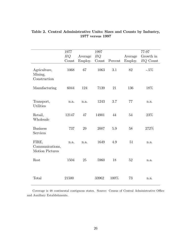
Table 2. Central Administrative Units: Sizes and Counts by Industry,1977 versus 1997

1977 1997 77-97HQ Average HQ Average Growth inCount Employ. Count Percent Employ. HQ Count

Agriculture, 1068 67 1063 3.1 82 -.5%Mining,Construction

Manufacturing 6044 124 7139 21 136 18%

Transport, n.a. n.a. 1243 3.7 77 n.a.Utilities

Retail, 12147 47 14901 44 54 23%Wholesale

Business 737 29 2007 5.9 58 272%Services

FIRE, n.a. n.a. 1649 4.9 51 n.a.Communications,Motion Pictures

Rest 1504 25 5960 18 52 n.a.

Total 21500 33962 100% 73 n.a.

Coverage is 48 continental contiguous states. Source: Census of Central Administrative Office

and Auxiliary Establishments.

26

Table 3. Entry and Exit of HQ’s

Entry Rate Exit Rate

77-82 .55 .48

82-87 .64 .53

87-92 .57 .52

92-97 .62 .53

Covers construction and mining (SIC 1), manufacturing (SIC 2 and 3), retailing and wholesaling

(SIC 5), and services (SIC 7 and 8, except for 80, 82, and 86). Entry is appearance of a new HQ in a

county, based on new company-plant identifier (excludes within county movers and auxiliaries which

change from non-HQ to HQ status). Source: Census of Central Administrative Office and Auxiliary

Establishments.

27

Table 4. National Share of Counties by Group in 1997

Ranked RestTop 10 11-75 Urban Rural

national private employment share .153 .290 .394 .163

national HQ employment share .211 .392 .343 .054relative to total emp. share 1.379 1.352 .871 .331

national services emp. share .219 .375 .335 .071relative to total emp. share 1.431 1.293 .850 .436

national manufacturing emp. share .133 .207 .402 .257relative to total emp. share .869 .714 1.020 1.577

U.S. counties are ranked by employment and aggregated into the four groups. The group share of

the national sector total is followed by the sector share relative to the total employment share. Sources:

County Business Patterns and Census of Central Administrative Office and Auxiliary Establishments.

28

Table 5. Importance of Out-Sourcing to HQ in 1997

a) Percent of HQ Units that Out-Source

Propensity

Accounting 58%

Legal 64%

Advertising 54%

b) Out-Sourcing Expenditures as a Fraction ofHQ Wage Bill For Out-Sourcers

Expenditures

Accounting 13.4%

Legal 15.2%

Advertising 36.6%

Source: Census of Central Administrative Office and Auxiliary Establishments.

29

Table 6. Ordinary and Fixed Effect Poisson Results(Births from t to t+ 1)

Ordinary Poisson Fixed Effects Poisson(1) (2) (3) (4) (5) (6)

ln(HQ wage in t) .0329 .00756 .0212 -.120∗∗ -.112∗∗ -.106∗∗

(.0396) (.0418) (.0420) (.0243) (.0241) (.0241)

wage index (t) -.195∗ -.218∗ -.147 -.426∗∗ -.426∗∗ -.436∗∗

business services (.117) (.129) (.123) (.0582) (.0582) (.0583)

diversity index (t) .377∗∗ .852∗∗ .651∗∗ .695∗∗ .657∗∗ .470∗∗

business services (.0572) (.0341) (.0637) (.0323) (.0305) (.0359)

wage index (t) .958∗∗ 1.50∗∗ 1.67∗∗ -.340∗∗ -.333∗∗ -.313∗

financial services (.272) (.304) (.302) (.160) (.160) (.160)

diversity index (t) -.763∗∗ .149 -.115 .551∗∗ .460∗∗ .00057financial services (.188) (.218) (.202) (.118) (.116) (.124)

ln(number HQ in t) .701∗∗ -.0908∗∗

(.0546) (.0241)

inverse(HQ in t) -4.44∗∗ -4.11∗∗ .280 .702∗∗

(.540) (.524) (.262) (.263)

ln(county employ.) .260∗∗ .561∗∗

(.0591) (.0563)

time-industry dummies yes yes yestime dummies yes yes yescounty-ind. fixed effects yes yes yesobservations 4345 4345 4345 4140 4140 4140counties 490 490 490 446 446 446Pseudo R2 .73 .71 .71

Standard errors are in parenthesis. Two ** indicate significance at 95%, one * at 90%.

30

Table 7. GMM Overall Results (Births from t to t+ 1)

GMM(1) (2) (3)

ln(HQ wage in t) -.326∗∗ -.341∗∗ -.329∗

(.161) (.161) (.174)

wage index (t) -.447∗∗ -.396∗∗ -.531∗∗

business services (.155) (.164) (.164)

diversity index (t) .461∗∗ .470∗∗ .519∗∗

business services (.084) (.0907) (.101)

wage index (t) -.489 -.507 -.343financial services (.412) (.410) (.450)

diversity index (t) .464∗ .468∗∗ .426∗

financial services (.258) (.236) (.252)

ln(number HQ in t) .308∗∗ .978∗∗

(.107) (.392)

inverse(HQ in t) -6.00∗∗

(1.63)

ln(HQ in t) squared -.0999∗∗

(.0449)

time dummies yes yes yesobservations 2812 2812 2812counties 429 429 429Sargan value 47.68 45.63 43.50p-value .364 .446 .578

Standard errors are in parenthesis. Two ** indicate significance at 95%, one * at 90%.

31

Table 8. Estimates of the Elasticity of HQ Scaleand the Need for Service Input Diversity

Estimate Standard Error

need for business services diversity (ρB) .492 .0732

need for financial services diversity (ρF ) .513 .182

elasticity of HQ scale (ε), linear form .174 .0627

elasticity of HQ scale, declining formevaluated at HQ = 1 3.46 1.11

HQ = 60 .0576 .0184HQ = 133 .0260 .00831

elasticity of HQ scale, quadratic formevaluated at HQ = 1 .526 .210

HQ = 60 .0858 .0622HQ = 133 .000349 .0693

Standard errors are calculated with the delta method using the covariance matrix from the second

stage of the Table 7 GMM regressions.

32

Table 9. GMM Other Scale Effects (Births from t to t+ 1)

(1) (2) (3) (4)ln(HQ wage in t) -.309∗ -.366∗∗ -.374∗∗ -.337∗∗

(.187) (.125) (.126) (.160)

business wage index (t) -.465∗∗ -.486∗∗ -.493∗∗ -.418∗∗

(.159) (.159) (.160) (.189)business diversity index (t) .466∗∗ .518∗∗ .521∗∗ .492∗∗

(.0933) (.0898) (.0900) (.0977)

finance wage index (t) -.441 -.663∗ -.654 -.558(.424) (.399) (.399) (.419)

finance diversity index (t) .450 .489∗ .498∗ .492∗∗

(.274) (.260) (.261) (.248)

ln(number HQ in t) .232∗∗

(.113)inverse(HQ in t) -5.55∗∗ -5.51∗∗ -6.05∗∗

(1.79) (1.80) (1.64)

ln(county employment) .241∗ .209(.134) (.152)

ln(PMSA population) .0987(.231)

ln(market potential) .365(.673)

ln(average employment .0895per HQ) (.0973)

time dummies yes yes yes yesobservations 2812 2812 2812 2812counties 429 429 429 429Sargan value 45.99 47.52 47.42 44.51Sargan p-value .390 .331 .297 .450

Standard errors are in parenthesis. Two ** indicate significance at 95%, one * at 90%.

33

Table 10. Summary Statistics

Variable Mean Standard Deviation

births 11.67 23.08

ln(HQ wage) 3.21 .403

business wage index 2.59 .297

business diversity index 3.29 1.10

finance wage index .379 .105

finance diversity index .444 .194

ln(number HQ) 2.09 1.28

(lnHQ)2 12.70 8.41

ln(HQ in rest of PMSA) 2.28 2.35

business diversity index in rest of PMSA 2.26 2.22

financial diversity index in rest of PMSA .305 .329

ln(county employment) 11.54 .938

ln(PMSA population) 13.29 1.14

ln(average employment per HQ) 7.11 1.73

34

Figure 1: HQ Establishments Location Quotientfor 1997 Counties

Rel

ativ

e S

hare

of H

Q E

stab

lishm

e

Log County Total Establishments

4 6 8 10 12

0

1

2

3

4

Observations include urban counties and are actually for all auxiliaries, which is public data.

This graph looks very similar to one that includes only HQ. The HQ establishments relative share, or

location quotient, is the ratio of the county’s share in national HQ establishments to the county’s share

of total national establishments in all industries. Note that the curves in the lower left portion of the

graph are due to the discrete nature of the establishment data. For example, one HQ establishment

is a uniformly increasing share in total establishments in this way as the size of the county becomes

smaller. Source: County Business Patterns.

35