The Cost of Dissolving the WTO:The Role of Global Production Networks

Mostafa Beshkar

Indiana University

Ahmad Lashkaripour

Indiana University

April 2020

Abstract

As trade agreements face renewed pressure, we show that the rise of global

production networks has multiplied the value of trade agreements to unprece-

dented levels. We cast our argument using a non-parametric neoclassical trade

model that accommodates global production networks and nests a wide class

of quantitative trade models as a special case. To guide our analysis, we de-

rive analytic formulas for optimal non-cooperative trade taxes in this general

framework. These formulas govern the extent of trade restriction if global

trade agreements were to dissolve. Mapping these formulas to data, we quan-

tify the value of trade agreements for various countries. We find that the disin-

tegration of existing trade agreements will erase 30% of the overall gains from

trade, which amounts to a $2.7 trillion loss in global GDP. Around 41% of this

value is driven by the agreements’ promotion of global production networks.

1 Introduction

Over the past few years, the tides have slowly turned against the WTO and otherfree trade agreements (Irwin (2020)). The rebirth of American unilateralism andconcerns over the erosion of national sovereignty have put the WTO and othertrade agreements at a critical cross road.1

1See https://www.cfr.org/backgrounder/whats-next-wto for a synthesis of common criti-cisms facing the WTO and other free trade agreements.

1

Experts have reacted to these developments with two opposing views: (1)One opinion is that trade agreements are more crucial than ever because a returnto protectionism will disrupt global production networks. (2) A somewhat con-trary opinion is that, given their increased reliance on global production networks,countries have little incentive to restrict foreign trade. So, it is conceivable thatsovereign governments would maintain the free flow of goods in and out of theircountry without a need for existing agreements.

While these opinions gain traction in political circles, we lack the necessary ev-idence to asses them. On one hand, the trade literature has directed most of itsattention to measuring the gains from trade relative to autarky. These measures donot speak to the value of free trade agreements, since a collapse of existing agree-ments will not necessarily lead to autarky (Costinot and Rodríguez-Clare (2014)).On the other hand, existing studies that focus on the pure gains from trade agree-ments overlook the role of global production networks.2

This paper aims to fill this gap. We present a general theory that describes howthe globalization of production networks has altered governments’ incentives vis-à-vis trade restrictions. We map our theory to data, to determine the counterfac-tual level of trade restriction and the efficiency loss that will occur without existingagreements. We find that the disintegration of existing trade agreements will erase30% of the overall gains from trade, which amounts to a $2.7 trillion loss in globalGDP. Around 41% of this value is driven by trade agreements facilitating the glob-alization of production networks.

Our analysis builds on Bagwell and Staiger’s (1999) insight that trade agree-ments solely “remedy the inefficient terms-of-trade-driven restrictions in trade that arisewhen trade policies are set unilaterally.” Based on this insight, the counterfactuallevel of trade restriction (without trade agreements) can be determined using theoptimal non-cooperative trade tax schedule in each country. Such a tax scheduledescribes the best-response of each country to the vector of trade taxes chosen byits trading partners. Solving the best-response functions simultaneously for allcountries, determines the terms-of-trade-driven trade restrictions that will occur inthe post-agreement Nash equilibrium.

2Ossa (2014) provides the most sophisticated analysis of the gains from trade agreements todate. His analysis presents a notable advance over prior analyses of the “gains from trade agree-ments” but it abstracts from global production networks.

2

Unfortunately, the existing literature does not provide a formal characterizationof optimal non-cooperative trade taxes in the presence of global production net-works. Existing characterizations of optimal trade taxes are either derived withinpartial equilibrium frameworks or abstract from global production networks.

To bridge this gap, we first present an analytical characterization of optimaltrade policy in a general equilibrium non-parametric neoclassical trade model thataccommodates (i) an arbitrary number of industries, (ii) an arbitrary demandstructure, (iii) an arbitrary global input-output network, and (vi) diseconomiesof scale due to industry-specific factors of production. Our general model nestsan important class of quantitative trade models, including the widely-used multi-industry gravity model with input-output linkages in Caliendo and Parro (2014).

Our characterization delivers simple sufficient statistics optimal tax formulasthat depend on only (i) industry-level trade elasticities, (ii) share of industry-specific capital in production, and (iii) observable expenditures, revenue, andinput-output shares. These formulas highlight three stark patterns:

(a) Absent diseconomies of scale, the optimal non-cooperative policy consists of(i) uniform or zero import taxes, and (ii) non-zero export taxes that are de-creasing in the industry-level trade elasticity and level of upstreamness.3

(b) But if export taxes cannot be used due to institutional constraints, import taxescan be employed as a second-best instrument to manipulate export marketpower through the global production network.

(c) Optimal second-best import taxes are targeted primarily at imported in-termediates, which are subsequently used in the production of highly-differentiated exports.4 They are uniform across all final and intermediate

3The redundancy of import taxes drives from the targeting principle and the Lerner symmetry.Absent diseconomies of scale, Home can only manipulate its import market power on an economy-wide basis. Doing so asks for a uniform tariff that (by the Lerner symmetry) can be perfectlymimicked with a uniform shift in all export taxes. By the targeting principle, import taxes are notthe first-best instrument for manipulating export market power either. So, altogether, they can bediscarded. Export taxes, meanwhile, are the first-best instrument for manipulating industry-levelexport market power. Optimal export taxes are decreasing in the industry-level trade elasticity,which governs the degree of export market power. They are relatively lower on upstream industriesthat supply intermediate inputs, because an export tax on intermediate inputs is partially passedback to domestic consumers. Finally, the absence of diseconomies of scale is akin to the completetariff passthrough estimated by Fajgelbaum et al. (2020) and Amiti et al. (2019).

4To elaborate, import taxes on intermediates are partially passed on to foreign consumers

3

goods that are never employed in exporting industries.

The above tax structure optimizes a non-cooperative government’s ability to cor-rect two unilateral terms-of-trade-related inefficiencies: (i) unexploited importmarket power, which concerns the unexploited ability of the Home country tocharge a mark-down on the price of imported goods; and (ii) unexploited exportmarket power, which concerns the unexploited ability of the Home country tocharge a mark-up on the price of exported goods. Correcting these two inefficien-cies is unilaterally optimal, but is detrimental to global efficiency and has beggar-thy-neighbor effects on the rest of the world.

Our theory indicates that the globalization of production networks has tiltedthe terms-of-trade-driven motives for taxation in two opposite directions: On onehand, global production networks prompt governments to set a lower export taxon upstream industries, because a fraction of this tax is passed back to domes-tic consumers. On the other hand, if governments cannot use export taxes, globalproduction networks prompt them to set a higher import tariff on upstream indus-tries, because these tariffs are partially passed on to Foreign consumers.5 In thatcase, import tariffs can serve as a second-best export policy measure. The empiricalsignificance of these two effects depends on the global input-output structure andthe size of the tax-imposing country compared to the rest of the world.

In Section 6 we map our analytic formulas to data to measure both the con-sequences of non-cooperative trade policies and the value of the agreements thatremedy them. To this end, we employ data on applied tariffs, expenditure, pro-duction, and input-output shares across 16 industries and 42 major economies.Our data includes all 27 members of the European Union, Australia, Brazil, China,Indonesia, India, Japan, Korea, Mexico, Norway, Russia, Switzerland, Taiwan,Turkey, the United States, and an aggregate of the rest of the world.

With the aid of our sufficient statics tax formulas, the task of computingthe value of trade agreements reduces to solving a system of equations that re-quires data on only (i) industry-level trade elasticities, (ii) observable expendi-

through the global production network. The more-intensively an imported intermediate is usedin the production of differentiated export goods, the higher the incidence of its tax on Foreign con-sumers. The trade-off, though, is that taxing intermediate inputs to mimic export taxes, distortsdomestic production in a way that is avoidable with first-best export taxes.

5Bown, Conconi, Erbahar, and Trimarchi (2020) confirm these cascading effects empirically,showing that tariffs in upstream sectors have large effects on prices, employment, sales, and in-vestment in downstream sectors.

4

ture/revenue shares, and (iii) global input-output shares. Our quantitative analy-sis delivers four basic results:

i. The globalization of production networks has only modestly reduced theterms-of-trade-driven incentives to restrict trade. Correspondingly, due to cas-cading effects, the gains from non-cooperative trade taxation and the exter-nality inflicted by these taxes on the rest of the world have doubled in thepresence of global production networks.

ii. Import taxes are significantly less effective at manipulating the terms-of-trade compared to first-best export taxes. They can only replicate 47% of theunilateral gains attainable under first-best export tax schedule. The ineffec-tiveness of second-best import taxes is driven by an innate trade-off betweenpreserving allocative efficiency in the local economy and exploiting exportmarket power through the production network. The former discourages tax-ing differentiated intermediate inputs, while the latter requires it.

iii. Existing trade agreements contribute $2.7 trillion to global GDP by reme-dying the inefficient terms-of-trade-driven restrictions in trade. To put thisfigure in perspective, it amounts to 30% of the total gains from trade relativeto autarky and equals the GDP of France.

iv. Around 41% of the above value drives from the agreements’ promotion ofglobal production networks. So, as the tides are starting to turn against freetrade agreements, their value has multiplied from the rise of global produc-tion networks.

Related Literature. To the best of our knowledge, this paper is the first to analyt-ically characterize the (unilaterally) optimal trade policy in an important class ofgeneral equilibrium quantitative trade models with global production networks.Several studies have adopted similar models to study the effect of global produc-tion networks on the gains from an exogenous tariff liberalization (e.g., Costinotand Rodríguez-Clare (2014); Caliendo and Parro (2014); Caliendo, Feenstra, Ro-malis, and Taylor (2015); and Baqaee and Farhi (2019)). But we are not aware ofany prior characterization of optimal trade policy in these canonical models.6

6There is an old literature that characterizes the optimal trade tax on intermediate inputs (e.g.,

5

Our characterization of optimal trade policy is related to Blanchard, Bown, andJohnson (2016) who characterize the optimal final-good tariff in a partial equilib-rium trade model under political economy considerations.7 Relative to the afore-mentioned study, our conceptual framework purposely precludes political pres-sures to isolate the terms-of-trade motives behind trade taxation. We, however,accommodate a wide range of general equilibrium linkages, analyzes both importand export taxation, and place no restrictions on how trade taxes discriminate be-tween final or intermediate input varieties of the same good. These extensions al-low us to identify a set of new insights that have eluded the prior literature on thistopic. Relatedly, our result on the uniformity (and therefore redundancy) of opti-mal tariffs generalizes similar results in Costinot, Donaldson, Vogel, and Werning(2015) and Opp (2010) to a non-parametric neoclassical trade model that accom-modates global input-output networks.

We also contribute to a recent literature that quantifies the gains from multilat-eral trade agreements. Ossa (2014, 2016) highlight the importance of market im-perfections when quantifying the gains from trade agreements. Bagwell, Staiger,and Yurukoglu (2018) highlight the importance of inter-connected bilateral negoti-ations. Carballo, Handley, and Limão (2018) analyze the role of trade agreementsat mitigating policy uncertainty. We contribute to this literature by measuring thecontribution of global production networks to the value of trade agreements.

Another strand of literature has used the structural gravity approach to mea-sure the value of free trade agreements (e.g., Baier and Bergstrand (2007); Egger,Larch, Staub, and Winkelmann (2011); Anderson and Yotov (2016)). This literaturetakes a different approach from ours and the quantitative studies listed above. It(a) models the economy as one industry, and (b) uses the estimated gravity coef-ficients to infer the counterfactual level of trade restriction in the absence of tradeagreements. While this approach has many merits, it is not optimized to accountfor global production networks—mostly, due to the single-industry nature of thestructural gravity model (see Limão (2016) for a review of this approach).

Suzuki (1978); Das (1983)). This literature typically assumes a three-good, partial equilibrium econ-omy with only one intermediate good that is produced in only one country. These frameworks, as aresult, do not feature a global production network in its formal sense, and deliver starkly differentpredictions relative to our framework.

7Relatedly, Grant (2019) studies the role of Special Economic Zones using an enriched partial equi-librium trade policy model where buyers are possibly heterogenous and the government appliesimport tariffs on many intermediate and final good varieties.

6

2 The Economic Environment

We consider a global economy that consists of i = 1, ..., N countries (with C de-noting the set of countries) and k = 1, ..., K industries (with K denoting the setof industries). Each country i is populated with Li workers that are perfectly mo-bile across industries but immobile across countries. Li,k denotes the number ofworkers employed in industry k. In addition to labor, each industry in country i isendowed with Ki,k units of industry-specific capital that is inelastically supplied.

Industry k ∈ K in country i ∈ C produces a differentiated variety that is ulti-mately sold in some market j ∈ C. We use ij, k (origin i–destination j–industry k)to index these product varieties. We use the superscript C to designate if a goodis used as a final consumption good and superscript I to designate of its used asan intermediate input. Since we impose no restrictions on the size or the num-ber of industries, we can interpret index k as denoting narrowly-defined productcategories rather than broadly-defined industries.

2.1 Preferences

The representative consumer in country i chooses the vector of consumption quan-tities, qCi ≡ qCji,k, to maximize a non-parametric utility function, Ui(qCi ), subjectto their budget constraint. The superscript C, as noted earlier, differentiates be-tween final consumption varieties and intermediate input varieties, with the latterdenoted by I . The optimal consumption choice yields the following indirect utilityfunction,

Vi(Yi, pCi ) ≡ maxqCi

Ui(qCi )

s.t. ∑k∈K

∑j∈C

(pCji,kqCji,k

)= Yi. (1)

The same probelm also yields a non-parametric Marshallian demand function,

qCi = Di(Yi, pCi ),

which summarizes the demand-side of the economy as a function of net consump-tion income Yi and the vector of consumer prices pCi ≡ pCji,k in country i. Thetilde notation on the price variables is used to differentiate the after-tax final price

7

from pre-tax producer price. To keep track of optimal demand choices, we definethe price and income elasticities of demand as follows.

D1. [Marshallian Demand Elasticities](i) [own price elasticity] ε ji,k ≡ ∂ ln qCji,k/∂ ln pji,k;

(ii) [cross-price elasticity] εi,gji,k ≡ ∂ ln qCji,k/∂ ln pi,g for i, g , ji, k;

(iii) [income elasticity] ηji,k ≡ ∂ ln qCji,k/∂ ln Yi.

Throughout this paper we restrict our attention to well-behaved demand func-tions that are continuous and locally non-satiated. We also assume that demandfor each traded variety exhibits an elastic region where | ε ji,k |> 1. As in monopolyproblems, this condition will be necessary for obtaining a bounded solution foroptimal trade taxes.

2.2 Technology

We assume that firms are competitive and operate with a non-parametric produc-tion function that employs (i) labor, (ii) intermediate inputs, and (iii) industry-specific capital. To elaborate, let Qi,k = ∑j τij,kqij,k denote country i’s total outputin industry k, where τij,k ≥ 1 accounts for the iceberg melt cost associated withtransporting variety ij, k—as is standard in literature, we normalize τii,k = 1. Theindustry-level output is produced using a general constant returns to scale pro-duction function,

Qi,k = Fi,k(Li,k, Ki,k, qIi,k),

that combines labor, Li,k, industry-specific capital, Ki,k, and intermediate inputs,qIi,k.8 We assume that the share of labor plus industry-specific capital is constant intotal production and equal to αi,k. However, we take no parametric stance on howlabor and capital are combined or how different intermediate inputs are combinedin the production function.

Facing the above production structure, cost-minimizing firms charge a com-petitive “producer” price that is a function of (i) the wage rate in economy i, wi,(ii) the vector of intermediate input prices employed by producers in country i,

8The above production structure implicitly assumes a non-finite elasticity of transformationbetween varieties sold in different markets. Relaxing this assumption will lead to diseconomies ofscale at the good rather than industry level (see Powell and Gruen (1968)).

8

pIi ≡ pIji,g, and (iii) total industry-level output, Qi,k. Namely,

pij,k = τij,kCi,k(wi, pIi ; Qi,k), (2)

where Ci,k(.) is homogeneous of degree 1 with respect to wi and pIi . A familiarspecial case of this general structure is the Ricardian case in which Ci,k (.) = ai,kwi,where ai,k is a constant unit labor cost that is invariant to industry-level output.

Cost minimization by suppliers in industry k of country i yields an industry-level demand function for intermediate inputs, Di,k(Yi,k, pIi ), which depends ongross expenditure on intermediate inputs, Yi,k ≡ ∑n(1− αi,k)pin,kqin,k, and the en-tire vector of intermediate input prices in country i. Country i’s overall demandfor intermediate inputs, qIi ≡ qIji,k, is determined as the sum of demands acrossall industries:

qIi = ∑kDi,k(Yi,k, pIi ).

For notational convenience, we assume that the after-tax price of product, ji, k, isthe same whether it is used as an intermediate input (indexed I) or a consumptiongood (indexed C):

pIji,k = pCji,k = pji,k.

This assumption is innocuous since we can always extend the set of goods so thatji, k indexes only the final good varieties, while ji, k′ indexes only the intermediateinput varieties supplied by the same industry.9 With the same rationale, we alsoassume that for all k, Di,k(.)/∂ lnYi,k = ∂ lnDi(.)/∂ ln Yi and ∂ ln Di,k(.)/∂ ln pIi =

∂ lnDi(.)/∂ ln pCi .We use input-output shares to keep track of global production networks. To

define these shares, let qI`i,g(k) denote the optimal amount of input `i, g used by in-dustry k in country i—by construction, qI`i,g = ∑k qI`i,g(k). Considering this choiceof notation, we define the global input-output shares as follows.

D2. [Input-Output Shares] The share of intermediate input goods from “country`×industry g” that are used in the production of output goods in “country j×industry

k” is defined as α`,gi,k ≡

pI`i,gqI`i,g(k)∑j pij,kqij,k

.

9Following this argument, our model still accommodates cases where the government imposesdifferential tax rates on final good varieties (k) versus intermediate input varieties (k′).

9

To be clear, we do not impose that input-output shares be constant. Instead,α’s can be variable, and will presumably change in response to trade taxation, e.g.,taxing input `i, g will lower α

`,gi,k . Our input-output setup is also flexible enough to

allow for the expenditure share on the intermediate input varieties of a given goodto diverge from the expenditure share on its final good varieties. A well-knownspecial case of our general input-output structure is Caliendo and Parro (2014),which we formally discuss in Section 4.1.

We use the supply elasticity, as defined below, to keep track of diseconomies ofscale at the industry level.

D3. [Industry-Level Supply Elasticity] γi,k ≡ ∂ ln Ci,k(.)/∂ ln Qi,k

The above definition is motivated by the observation that Ci,k(..., Qi,k) charac-terizes the industry-level supply curve for country i. To gain intuition about howthis elasticity relates to diseconomies of scale, consider the case where the shareof the industry-specific capital in production is constant and equal to βi,k. In thatcase, it is straightforward to show that γi,k = βi,k/(1− βi,k). Beyond this special,γi,k still reflects the importance of the inelastically-supplied capital in production.As we will see shortly, γi,k also governs the degree of national-level import marketpower in each industry.

2.3 Trade Policy Instruments

The government in country i has access to a full set of industry-level export tax-cum-subsidy instruments (denoted by x) and import tax-cum-subsidy instruments(denoted by t). Together, these policy instruments create a wedge between theafter-tax price, pji,k, and the producer price, pji,k, of each good ji, k as follows:

pji,k =(1 + tji,k

) (1 + xji,k

)pji,k. (3)

In the above equation, tji,k denotes the import tax applied by country i on goodji, k, while xji,k denotes the export tax applied by country j on the same good. Thecombination of these tax instruments raises the following tax revenue for the gov-ernment in country i:

Ri = ∑k∈K

∑j∈C

[tji,k

(1 + xji,k

)pji,kqin,k + xij,k pij,kqij,k

]. (4)

10

Tax revenues are rebated to the consumers in a lump-sum fashion.10 Throughoutthis paper, we assume that domestic policies are unavailable, which amounts totii,k = xii,k = 0 for all i and k. As noted earlier, our product space is general enoughthat k can index only the final good version or the intermediate input version ofeach industry’s output. So, in principle, trade taxes can arbitrarily discriminatebetween final consumption and intermediate input varieties of the same good.

2.4 General Equilibrium

We assume throughout this paper that equilibrium is unique—noting that unique-ness can be formally established using the procedure in Alvarez and Lucas (2007).Below, we formally define the general equilibrium in our setup.

Definition. For any given vector of taxes, t, and, x, equilibrium is a vector of wages,w, (pre-tax) producer and (after-tax) final prices, pi, and pi, final consumption and inputdemand choices, qCi and qIi , total surplus paid to industry-specific capital, Π, net consumerexpenditure, Y , and gross industry-level output, Y , such that (i) the producer price foreach good is characterized by Equation 2; (ii) the consumer price for each good is given byEquation 3; (iii) consumption choices, qCi = Di (Yi, pi), are a solution to 1; (iv) demandfor intermediate inputs, qIi = ∑k Di(Yi,k, pIi ), is chosen to minimize cost; (iv) factormarkets clear

wiLi + Πi = ∑j

∑k

pij,kqij,k −∑j

∑k

pIji,kqIji,k ∀i,

and (v) net consumption income equals factor income plus tax revenue

Yi = wiLi + Πi +Ri ∀i,

where the tax revenue,Ri, is given by Equation 4.

To streamline the presentation of our theory, we henceforth express aggregatewelfare in country i as a function of taxes t, and, x, and wages, w,

Wi (ti, xi; t−i, x−i, w) ≡ Vi (Yi(ti, xi; t−i, x−i, w), pi(ti, xi; t−i, x−i, w)) .

10Since labor is inelastically supplied in our framework, lump-sum rebates are observationallyequivalent to a wage subsidy or a uniform consumption subsidy.

11

w is an equilibrium outcome and, thus, an implicit function of trade taxes, So,we use A to denote the set of all wage×policy combinations, A = (t, x; w), thatare feasible. The reason we express Wi as a function of (t, x; w) rather than justtrade taxes is that an across-the-board shift in trade taxes combined with an equal-proportional adjustment to nominal wage rates preserves welfare. Expressingequilibrium outcomes in terms of the triplet (t, x; w) enables us to track this kindof tax neutrality.

In equilibrium, the importance of each good for taxation purposes is deter-mined (among other things) by its share in gross expenditure and output. So be-fore concluding this section, it is useful to define the aforementioned shares forgood ji, k (origin j–destination i–industry k).

D4. [Gross Expenditure and Output Shares][within-industry expenditure share] λji,k ≡

pji,kqji,k∑∈C pi,kqi,k

[overall expenditure share] λji,k ≡pji,kqji,k

∑∈C ∑g∈K pi,gqi,g.

[within-industry output share] rji,k ≡pji,kqji,k

∑ι∈C pjι,kqjι,k

[overall output share] rji,k ≡pji,kqji,k

∑ι∈C ∑g∈K pjι,gqjι,g

Gross expenditure and output shares, as defined above, are directly observablein standard trade datasets. As we well see shortly, optimal trade taxes can be fullycharacterized in terms of these observable shares plus input-output shares and thereduced-form demand and supply elasticities defined earlier.

3 Unilaterally Optimal Trade Taxes

We begin our analysis by characterizing the unilaterally optimal tax schedule ineach country given applied taxes in the rest of the world. Since our analysis pre-cludes political economy motives, the aforementioned taxes are purely terms-oftrade-driven. So, following Bagwell and Staiger (1999), they govern the efficiencyloss that free trade agreements are designed to remedy.11

11Our analysis fits into the terms-of-trade framework, wherein trade agreements “remedy the inef-ficient terms-of-trade-driven restrictions in trade that arise when trade policies are set unilaterally, (Bagwelland Staiger (1999))” Based on this viewpoint, the value of free trade agreements can be measured asthe reduction in trade that would otherwise occur if countries were imposing terms-of-trade-drivenrestrictions in trade. See also Maggi and Rodriguez-Clare (1998); ? for a domestic-commitment theoryof trade agreements.

12

For expositional purposes, we cast our theory first using a two-country setupwhere h indexes the Home country and f indexes Foreign that represents an ag-gregate of the rest of the world, i.e., C = h, f . Later, in Section 4.2 we showhow our baseline results extend to a multi-country setup with arbitrarily manycountries. The Home government’s optimal non-cooperative policy, t∗h ≡ t∗f h,k,and x∗h ≡ xh f ,k, solves the following problem taking the vector of Foreign taxes,t f ≡ th f ,k, and x f ≡ x f h,k, as given:

max(th,xh;t f ,x f ,w)∈A

Wh(th, xh; t f , x f , w

). (5)

It is needless to say that the above problem is complicated by a myriad of generalequilibrium interrelations. We can nonetheless simplify the problem by appealingto several intermediate results, the first of which is the Lerner symmetry.12

Lemma 1. [The Lerner Symmetry] For any a ∈ R+, combinations A =(1 + th, 1 + xh; t f , x f , wh, w f

)and A′ =

(a(1 + th), (1 + xh)/a; t f , x f , awh, w f

)rep-

resent identical equilibria, i.e., Wi(A) = Wi(A′) for all i .

The above lemma simplifies our analysis as follows: Optimal import and ex-port taxes both feature a uniform term that accounts for the ability of trade taxesto increase Home’s wage relative to Foreign (wh/w f ). Following the above lemma,we need not to formally characterize this term as it is redundant. There is an-other way to cast this redundancy: When both export and import taxes are appli-cable, Lemma 1 indicates that we can normalize wages in both economies (i.e., setwh = w f = 1) and still identify one of the multiple optimal tax combinations. Thisresult, however, follows only if a full set of industry-level export and import taxinstruments are applicable. If the policy space is restricted in any way, the uniformtax component that accounts for the general equilibrium changes in wh/w f shouldbe formally characterized—see Section 3.1 for further details.

In our general equilibrium setup, trade taxes have a non-trivial passthroughonto the vector of final prices, pi, in each country. A tax on one good can al-ter the entire vector of prices through its effect on country-level wages, inputprices, and industry-wide output. To handle these complex interrelations, we can

12See Costinot and Werning (2019) for a more comprehensive treatment of the Lerner symmetryin the presence of multinational firms, global imbalances, and imperfect competition.

13

cast our original optimal policy problem as one where the government directlychooses final prices, p f h, ph f , and phh, to maximize Home’s welfare Wh (p; w) ≡Vh (Yh(p; w), p). Stated formally, the optimal policy problem can be reformulatedas

max(p;w)∈A

Wh (p; w) ,

where A denotes the set of feasible wage-price combinations that is defined anal-ogously to A. Implicit in the above formulation is the observation that (i) Wh(.)does not explicitly dependent on p f f , and (ii) the market equilibrium is efficient,so it is optimal to set phh = phh. The above problem, as a result, corresponds toone where the government chooses the consumer-to-producer price wedges thatpin down the trade taxes: 1+ th = p f h/(1+ x f )p f h and 1+ xh = ph f /(1+ t f )ph f .

Finally, we can appeal to supply- and demand-side envelop conditions to han-dle general equilibrium behavioral responses. On the demand side, we can appealto Roy’s identity, whereby the direct welfare effect of a change on consumer price,pCf h,k, is reduced to ∂Vh(.)/∂ pCf h,k = −qCf h,k. Similarly, we can appeal to Shepard’slemma to account for input-output-driven price linkages. Specifically, a change ininput price pI`i,g, holding the wage and all other input prices fixed, has the follow-ing effect on the output price of a cost-minimizing supplier:

∂ ln pij,k

∂ ln pI`i,g=

∂ ln Ci,k(.)∂ ln pI`i,g

= α`,gi,k ,

where α`,gj,k denotes the share of input `i, g in output ij, k as defined by D3.

The change in pI`i,g has an additional general equilibrium effect, which operatesthrough changes in w, Y , and Y . As noted earlier, though, the handling of thesegeneral equilibrium effects can be simplified with the application of Lemma 1.

Trade taxes also affect, Πi, which is the surplus paid to industry-specific capitalin country i. To track this effect, we can appeal to Hotelling’s lemma, whereby theeffect of a change in output prices on surplus (holding all input prices constant) canbe stated as: ∂Πi(.)/∂pij,k = qij,k. Likewise, the effect of a change in the price ofintermediate input ji, k (holding the price of all other inputs fixed) can be expressedas: ∂Πi(.)/∂pIji,k = qIji,k.

By combining the aforementioned envelope conditions and appealing toLemma 1, we can produce the following theorem that characterizes the optimal

14

policy as a function of gross expenditure shares, λ, gross revenue shares, r, globalinput-output shares, α, reduced-form demand elasticities, ε, and reduced-formsupply elasticities, γ. The former three statistics are directly observable, while thelatter two can be locally estimated.

Theorem 1. Home’s unilaterally optimal trade taxes are unique up-to a uniform taxshifter, t, and given by

1 + t∗f h,k =

(1 +

γ f ,kr f h,k

1− γ f ,kr f f ,kε f f ,k

)(1 + t)

1 + x∗h f ,k =εh f ,k

1 + εh f ,k + ξh f ,k −∑g αh,kf ,g

r f h,g

λh f ,k

(1 + t)−1

where[ξh f ,k

]k =

[Ξ−1 − IK

]Ω accounts for input-output adjusted cross-demand effects

between industries, with Ξ ≡[

λh f ,gεh f ,kh f ,g

λh f ,kεh f ,k

]k,g

and Ω ≡[

1−∑g αh,kf ,g

r f h,g

λh f ,k

]k.

Foreign’s unilaterally optimal taxes are, analogously, described by a similar for-mula that swaps the country indices. As noted earlier, per the Lerner symmetry,the unilaterally optimal policy is unique only up to a uniform tariff, t. For a high-enough choice of t, the optimal policy will consist of import taxes paired withexport subsidies. Aside from the uniform tax shifter, Home’s unilaterally optimalimport tax, t∗f h,k, equals the optimal industry-level mark-down on p f h,k (i.e., the in-verse of the export supply elasticity). Home’s unilaterally optimal export tax, x∗h f ,k,is equal the optimal monopoly mark-up on ph f ,k that internalizes cross-demand ef-fects and tax propagation through the production network. In the special case withzero cross-substitutability between industries (i.e., Ξ = IK ⇐⇒ ξh f ,k = 0) and noinput-output networks (i.e., αh,k

f ,g = 0), the optimal export tax reduces to the famil-iar single-product optimal monopoly markup, 1 + x∗h f ,k = εh f ,k/

(1 + εh f ,k

).

Importantly, the optimal tax schedule specified by Theorem 1 internalizes For-eign’s applied taxes, t f , and x f . For instance, an increase in Foreign’s import taxeswill shrink Home’s exports to Foreign. This effect will reflect itself as a reductionin εh f ,k (and therefore x∗h f ,k) if the demand for variety h f , k is sub-convex. We can,thus, express t∗f h,k and x∗h f ,k as an implicit function of Foreign’s applied taxes. Wewill invoke this property in Section 5, where we solve for Nash taxes in the non-cooperative equilibrium.

15

Theorem 1 has an attractive feature: It characterizes the optimal policy in termsof estimable or observable sufficient statistics. In the words of Piketty and Saez(2013), such sufficient statistic formulas have two broad merits. First, they allowus “to understand the key economic mechanisms behind the formulas.” Second,they “are also often robust to changing the primitives of the model.” In the presentcontext, the formula characterized by Theorem 1 can be empirically evaluated withreadily-available trade statistics. Given these qualities and as shown later in Sec-tion 6, Theorem 1 streamlines the quantitative analysis of trade policy to a greatdegree.

There is a simple intuition for why optimal import taxes (unlike export taxes)do not explicitly depend on global input-output shares. From the perspective of theHome country, trade taxes can correct two terms-of-trade-related distortions:

i. Unexploited import market power, which concerns the unexploited ability ofthe Home economy to charge a mark-down on Foreign producer prices, p f h,k.

ii. Unexploited export market power, which concerns the unexploited ability ofthe Home economy to charge a mark-up on Foreign consumer prices, ph f ,k.

By the targeting principle, industry k’s optimal import tax, t∗f h,k, is targeted exclu-sively at lowering p f h,k (Margin 1). For this reason, t∗f h,k does not explicitly dependon input-output shares. To make this point, consider the following thought exper-iment: Fix the price of all of Home’s export goods as these prices can be directlymanipulated with export taxes. In that case, t f h,k cannot affect either p f h,g or ph f ,g through the input-output network. Instead, t f h,k can only lower p f h,k byshrinking Foreign’s output in industry k or by lowering w f . These effects, by con-struction, operates independent of the input-output network.

Based on the same rationale, optimal export taxes depend explicitly on globalinput-output shares. An export tax on intermediate input, h f , k, will raise the priceof any Foreign-produced good employing that input, including goods that are soldback to the Home country. That is, An export tax on intermediate inputs is par-tially passed back to Home consumers through re-importation. To mitigate theseadverse feedback effects, the optimal export tax is lower on more upstream indus-tries where re-importation of export taxes is more of an issue. This claim is implicit

16

in the formula under Theorem 1, considering that13

∑g

αh,kf ,g

r f h,g

λh f ,k∈

0 if f h, k is a final good

(0, 1) otherwise

That export taxes are lower on upstream industries, however, should not be con-fused with smaller gains from taxation. On the contrary, the unilateral gains fromtaxing upstream exports are actually larger. We formally document and discussthis point in Section 6.

Theorem 1 indicates that import taxes are a necessary instrument only if thereare diseconomies of scale arising from industry-specific capital. Otherwise, ifγ f ,k ≈ 0, Home can discard import taxes by choice of t = 0, and attain the first-bestnon-cooperative outcome with only export taxes. The following corollary synthe-sizes this claim and others discussed earlier.

Corollary 1. Holding λ and r constant, the globalization of production networks low-ers the unilaterally optimal export tax on more-upstream industries. Moreover, absentdiseconomies of scale, import taxes remain a redundant terms-of-trade-improving policyinstrument even after countries become immersed in global production networks.

The globalization of production networks, in the above corollary, correspondsto a counterfactual thought experiment where λ and r are fixed, but α is risenfrom zero to its factual level. This experiment aligns with the quantitative exer-cise presented later in Section 6. Corollary 1, therefore, indicates that overlookingglobal production networks will lead to an over-estimation of non-cooperative ex-port taxes in upstream industries.

Finally, the absence of diseconomies of scale is a sufficient but not necessarycondition for the redundancy of import taxes. Import taxes can be redundant un-der much weaker conditions. For instance, suppose Foreign employs industry-specific capital but Home accounts for a small share of global demand for the For-eign industry. Then, r f h,k ≈ 0 and import taxes are once again redundant. Theaforementioned situation provides an accurate description of any individual coun-try’s position relative to the rest of the world. It also aligns with the complete tariffpassthrough documented by Amiti et al. (2019) and Fajgelbaum et al. (2020).

13More generally, ∑g αh,kf ,g r f h,g/λh f ,k = 0 if good f h, k is not used as an input in any of Foreign’s

export goods. Final goods automatically satisfy this qualification.

17

3.1 Second-Best Non-Cooperative Import Taxes

We now consider a scenario that has received considerable attention in the priorliterature. In this scenario, governments cannot apply export taxes due to institu-tional constraints like those embedded in the United States’ constitution. But theyhave the discretion to apply import taxes. We show that, in such circumstances,it is unilaterally optimal for governments to use import taxes as a second-best in-strument to manipulate export market power. To make this point succinctly, weabstract from diseconomies of scale and cross-industry demand effects; but thesechannels are formally accounted for in Appendix C.

In a second-best scenario where the government cannot apply export taxes,Home’s unilaterally optimal import taxes solve the following problem (taking t f

and x f as given):max

(th,0;t f ,x f ,w)∈A

Wh(th, 0; t f , x f , w

).

Since export taxes are restricted to zero, i.e., xh = 0, the Lerner symmetry no longerimplies a multiplicity of optimal tax schedules. Instead, the above problem iden-tifies a unique vector of optimal import taxes. Since the Home economy possessesno import market power by assumption (i.e., γ f ,kr f h,k ≈ 0), second-best importtaxes pursue one objective: to indirectly manipulate Home’s export market power.

Export market power manipulation can be carried through two distinct chan-nels: First, import taxes can raise Home’s wage relative to Foreign, wh/w f (i.e.,they can charge a markup on the wage rate embedded in Home’s exports). Sec-ond, import taxes can be used to charge a markup on ph f ,k through the input-output network. The former channel was previously-redundant due to the Lernersymmetry-driven multiplicity of optimal taxes. The latter channel was also irrele-vant due to the targeting principle.

To account for the now-relevant general equilibrium wage effects, we useLij (t, x; w) to denote country j’s demand for country i’s labor. The elasticity of Lij

with respect to wi depends on the value-added content of sales, which determinesthe overall contribution of country i’s labor to gross revenue in each industry. Wecan measure the value-added content of country i’s output in industry k, namely,δi,k, using the input-output matrix. Specifically, let

αji ≡[α

j,gi,k

]k,g

18

denote the K × K input-output matrix that describes the share of country j’s in-puts used in country i’s outputs. We can apply the Implicit Function Theorem tocalculate δi ≡ [δi,k]k as follows:

δi = (IK − αii)−1 αi,

where αi ≡ [αi,k]k is a K× 1 vector denoting industry-level labor shares in countryi . Using the above notation, we can calculate the elasticity of labor demand interms of gross reduced-form demand elasticities, εij,k, and value-added shares, δi,k.

D4. [Elasticity of Labor Demand] εij ≡∂ lnLij∂ ln wi

= ∑k ωij,kεij,k, where ωij,k ≡δj,kλij,k

∑g δj,k rji,k

is a weight that reflects the value-added contribution of good ij, k to country i’s exports.

In principle, εij measures country i’s economy-wide export market power netof input-output linkages. As noted by the following Theorem, Home’s optimalimport tax in each industry is determined by εh f and an industry-specific termthat accounts for the ability of import taxes to manipulate industry-specific exportmarket power through the production network.

Theorem 2. In a second-best scenario where export taxes are inapplicable, unilaterallyoptimal import taxes feature of a uniform component and an industry-specific competentthat captures the extent to which import taxes are passed on to Foreign consumers. Namely,

1 + t∗f h,k =εh f

1 + εh f

(1 +

τkε f h,k

),

where τ ≡ [τk] is given by

τ =

1k=g +ε

hh,gf h,g

ε f h,kα

f ,kh,g

−1

k,g

[∑

g∈K

(α

f ,kf ,g − [1 +

εh f ,g

εh f]λh f ,g

r f h,gα

f ,kh,g

)]k

,

with[α

f ,kf ,g

]k,g

=(

IK − α f f)−1

α f hαh f , and[α

f ,kh,g

]k,g

=(

IK − α f h)−1

α f h. Correspond-

ingly, τk = 0 for import goods that are not used as intermediate inputs in export goodsand τk , 0 otherwise.

The uniform term, εh f /(1 + εh f ), in the above formula, corresponds to an op-timal export mark-up on the wage rate, wh. To elaborate, a uniform import tax is

19

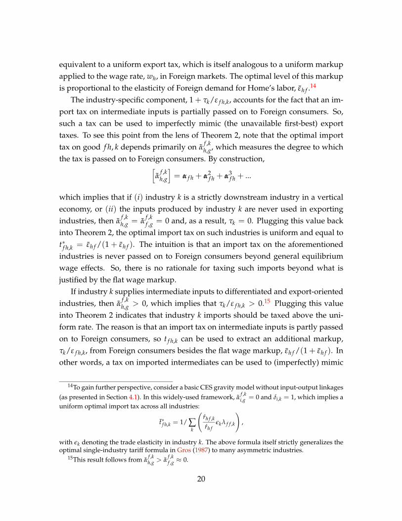
equivalent to a uniform export tax, which is itself analogous to a uniform markupapplied to the wage rate, wh, in Foreign markets. The optimal level of this markupis proportional to the elasticity of Foreign demand for Home’s labor, εh f .14

The industry-specific component, 1 + τk/ε f h,k, accounts for the fact that an im-port tax on intermediate inputs is partially passed on to Foreign consumers. So,such a tax can be used to imperfectly mimic (the unavailable first-best) exporttaxes. To see this point from the lens of Theorem 2, note that the optimal importtax on good f h, k depends primarily on α

f ,kh,g, which measures the degree to which

the tax is passed on to Foreign consumers. By construction,[α

f ,kh,g

]= α f h + α2

f h + α3f h + ...

which implies that if (i) industry k is a strictly downstream industry in a verticaleconomy, or (ii) the inputs produced by industry k are never used in exportingindustries, then α

f ,kh,g = α

f ,kf ,g = 0 and, as a result, τk = 0. Plugging this value back

into Theorem 2, the optimal import tax on such industries is uniform and equal tot∗f h,k = εh f /(1 + εh f ). The intuition is that an import tax on the aforementionedindustries is never passed on to Foreign consumers beyond general equilibriumwage effects. So, there is no rationale for taxing such imports beyond what isjustified by the flat wage markup.

If industry k supplies intermediate inputs to differentiated and export-orientedindustries, then α

f ,kh,g > 0, which implies that τk/ε f h,k > 0.15 Plugging this value

into Theorem 2 indicates that industry k imports should be taxed above the uni-form rate. The reason is that an import tax on intermediate inputs is partly passedon to Foreign consumers, so t f h,k can be used to extract an additional markup,τk/ε f h,k, from Foreign consumers besides the flat wage markup, εh f /(1 + εh f ). Inother words, a tax on imported intermediates can be used to (imperfectly) mimic

14To gain further perspective, consider a basic CES gravity model without input-output linkages(as presented in Section 4.1). In this widely-used framework, α

f ,ki,g = 0 and δi,k = 1, which implies a

uniform optimal import tax across all industries:

t∗f h,k = 1/ ∑k

(rh f ,k

rh fεkλ f f ,k

),

with εk denoting the trade elasticity in industry k. The above formula itself strictly generalizes theoptimal single-industry tariff formula in Gros (1987) to many asymmetric industries.

15This result follows from αf ,kh,g > α

f ,kf ,g ≈ 0.

20

the first-best export taxes.16 The trade-off is that taxing intermediate inputs dis-torts production decisions in a way that is avoidable with first-best export taxes.

In summary, these arguments indicate that the globalization of production net-works creates an additional incentive for import taxation in second-best scenar-ios. More specifically, if production networks become globalized and export taxesare inapplicable, it is unilaterally optimal to increase the import tariff on more-upstream industries. The following corollary synthesizes these arguments.

Corollary 2. Suppose export taxes are inapplicable: Holding λ and r constant, the glob-alization of production networks increases the unilaterally optimal tariff on upstream in-dustries that supply intermediates inputs to export-oriented sectors. The globalization ofproduction networks, however, has no effect on the unilaterally optimal tariff in industriesthat supply final goods or intermediate goods that are never used in export-oriented sectors.

The above corollary raises a basic question: How much are governments willing toraise the tariff on intermediate inputs to mimic export taxes? Answering this questionis ultimately a quantitative matter, which is explored in Section 6. But we can gainvaluable insights by approaching the question theoretically. If imported goodsare re-exported without being processed, then an import tax on these goods isidentical to an export tax. So the globalization of production-networks prompts asharp increase in optimal import taxes.

Beyond this extreme case, import taxes on intermediate inputs are an extremelyinefficient substitute for export taxes: First, they directly distort production-relatedchoices in the Home economy. Second, they may be partially passed on to domes-tic consumers. Accordingly, the effectiveness of second-best trade taxes is ham-pered by an innate trade-off between preserving allocative efficiency in the localeconomy and exploiting export market power through the production network.The former discourages taxing differentiated intermediate inputs, while the latterrequires it. As a result, for all practical purposes, the globalization of productionnetworks should have a modest effect on non-cooperative import taxes.

16Aside from αf ,kh,g, the effectiveness of t f h,k at mimicking first-best export taxes is governed by

two additional factors: (a) the degree to which intermediate input variety f h, k is substitutable withother inputs (i.e., ε f h,k in the formula specified by Theorem 2); and (b) the intensity at which input

f h, k is used in highly-differentiated export-oriented industries (i.e., αf ,kh,gλh f ,gεh f ,g in the formula

specified by Theorem 2). Specifically, t∗f h,k is higher if intermediate input f h, k is low-demand elasticand is used more-intensively in highly-differentiated, export-oriented industries. The followingcorollary summarizes these arguments.

21

4 Canonical Special Cases and Extensions

In this section, we first highlight two widely-used quantitative trade models thatare nested by our theory. We then demonstrate how our baseline results readilyextend to a multi-country setup.

4.1 Canonical Special Cases

To highlight the practicality of our optimal tax formula, we outline two canoni-cal special cases: First, a basic multi-industry gravity model without input-outputlinkages à la Costinot et al. 2011. Second, a multi-industry gravity model withflexible input-output linkages à la Caliendo and Parro (2014).

(i) Basic Multi-Industry Gravity Model (Costinot et al. 2011). This model corre-sponds to a special case of our framework where labor is the only factor of produc-tion and preferences have a Cobb-Douglas-CES parameterization: Ui = ∏k Qei,k

i,k ,

where Qi,k =(

∑j=h, f χji,kqρkji,k

)1/ρk. The Cobb-Douglas-CES demand structure im-

plies that εh f ,k = −1− εkλ f f ,k, where εk ≡ ρk/ (1− ρk). The Cobb-Douglass as-sumption also eliminates cross-price elasticity effects, which amounts to ξh f ,k = 0.

The absence of input-output networks implies that αf ,kh,g = 0 for a k and g. Plug-

ging these values into the optimal tax formula specified by Theorem 1 yields thefollowing:

1 + t∗f h,k = 1 + t

1 + x∗h f ,k =

(1 +

1εkλ f f ,k

)(1 + t)−1. (6)

Stated verbally, the optimal trade tax consists of a uniform tariff, t, and an industry-specific export tax that varies primarily with the industry-level trade elasticity, εk.If the economy is modeled as a single industry, the above formula reduces to x∗h f =

1/ελ f f , which by the Lerner symmetry is equivalent to Gros’ (1987) optimal tariffformula, t∗f h = 1/ελ f f .

(ii) Multi-Industry Gravity Model with I-O Linkages (Caliendo and Parro (2014))This model features the same CES-Cobb-Douglas utility function described above.

22

Production, though, combines intermediate inputs and labor using a Cobb-Douglas-CES aggregator, which implies that

pij,k = wαi,ki ∏

gP

αi,gki,g ,

where αi,kg denotes the constant share of industry k’s inputs in industry g’s out-put, with αi,k ≡ 1 − ∑g αi,gk. Pi,g denotes the (after-tax) price index of industryg’s composite intermediate input, which is by assumption identical to the price in-

dex of industry g’s composite consumption good: Pi,g =(

∑j p1−εgji,g

)1/(1−εg). The

Cobb-Douglas-CES demand for the consumption variety of good ji, k is qCji,k =(pji,k/Pi,k

)−εk ei,kYi. The demand for the intermediate input variety of good ji, k isgiven by qIji,k =

(pji,k/Pi,k

)−εk ∑g αi,kgYi,g.We can apply Theorem 1 along with the following steps to determine the opti-

mal trade tax in this setup: Since there are no industry-specific factors of produc-tion, we can set γ f ,k = 0 for all k. The Cobb-Douglas assumption meanwhileensures that ξh f ,k = 0. The within-industry CES demand system implies thatεh f ,k = −1− εkλ f f ,k. The assumption that the demand aggregator for final andintermediate goods are identical, entails that αh,k

f ,g = α f ,kgλh f ,k. Plugging these val-ues into Theorem 1 yields the following formula for optimal trade taxes in theCaliendo and Parro (2014) model:

1 + t∗f h,k = 1 + t

1 + x∗h f ,k =

(1 + εkλ f f ,k

εkλ f f ,k −∑g α f ,kgr f h,g

)(1 + t)−1 . (7)

In-line with our earlier discussion, the optimal export tax implied by the above for-mula is strictly lower than that implied by the baseline gravity model (Equation 6).However, the gains from optimal trade taxation are higher relative to the baselinemodel. This point is quantitatively established in Section 6 where we calibrate theabove formulas to actual data.

4.2 Extension to a Multi-Country Setup

We now extend our optimal tax formulas to a multilateral setup with N > 2 coun-tries. The optimal policy problem in this setup is a basic extension of 5: Country

23

i chooses (N − 1)K import tax instruments, ti = tji,k, and (N − 1)K export taxinstruments, xi = xij,k, given the vector of applied ‘taxes in the rest of the world,t−i, and x−i . 17 We can follow the same steps outlined earlier to derive sufficientstatistics formulas for optimal trade taxes in this setup (see Appendix D):

1 + t∗ji,k =

(1 +

γj,krji,k

1−∑ι,i γj,krjι,kε jι,k

)(1 + t)

1 + x∗ij,k =εij,k

1 + εij,k + ξij,k −∑g ∑,iΛi,g

Λij,kαi,k

j,g

(1 + t)−1. (8)

In the above formula, ξij,k accounts for cross-industry demand effects and is de-fined analogously to the cross-demand term specified under Theorem 1;18 Λi,g ≡pji,gqji,g/ ∑,i ∑k pi,kqi,k and Λij,g ≡ pij,gqij,g/ ∑,i ∑k pi,kqi,k denote import and

export shares; and[αi,k

j,g

]= αi

jαj if , j, with

[αi,k

jj,g

]= αi

j.The optimal tax formula specified above differs from the baseline formula (pre-

sented under Theorem 1) in one basic aspect. The optimal export tax accounts forthe fact that a tax on any individual export variety may be passed back to domesticconsumers through multiple partners. The term αi,k

j,g, in the denominator, accountsfor the extent to which xij,k is passed back to domestic consumers through country’s export of industry g goods. The higher the αi,k

j,g’s from various ’s, the lower theoptimal export tax. The same formula also indicates that the burden of an exporttax on one partner may be borne primarily by a third country that is not directlyinvolved in the export transaction.

This subtle difference notwithstanding, the claims presented under Corollaries1 and 2 readily extend to the multi-country case. As before, the optimal importtaxes do not explicitly depend on the global input-output shares, which is a man-ifestation of the targeting principle. Absent diseconomies of scale, import taxesare also uniform and, therefore, redundant under the first-best scenario.19 We

17An added complication here is that a tax on good ji, k can alter the entire vector of national-level wages w1, ...wN. This complication can be handled by noting that tji,k’s effect on Wi has afirst-order component that operates through changes in wj/wi and a second-order component thatoperates through changes in w/wi (where j , j)—see Appendix D.

18Stated formally, ξij,k is given by[ξij,k

]k=

[ λij,gεij,kij,g

λij,kεij,k

]−1

k,g

− IK

[1−∑g ∑Λi,g

Λij,kαi,k

j,g

].

19The uniformity of optimal tariffs across industries is independent of the first-order approxi-mation discussed in Footnote 10—see Appendix D for details.

24

also demonstrated how the characterization under Theorem 1 readily extends to amulti-country setup.

5 The Non-Cooperative Trade Equilibrium

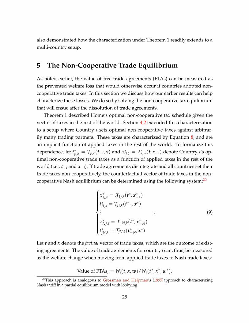
As noted earlier, the value of free trade agreements (FTAs) can be measured asthe prevented welfare loss that would otherwise occur if countries adopted non-cooperative trade taxes. In this section we discuss how our earlier results can helpcharacterize these losses. We do so by solving the non-cooperative tax equilibriumthat will ensue after the dissolution of trade agreements.

Theorem 1 described Home’s optimal non-cooperative tax schedule given thevector of taxes in the rest of the world. Section 4.2 extended this characterizationto a setup where Country i sets optimal non-cooperative taxes against arbitrar-ily many trading partners. These taxes are characterized by Equation 8, and arean implicit function of applied taxes in the rest of the world. To formalize thisdependence, let t∗ji,k = Tji,k(t−i, x) and x∗ij,k = Xij,k(t, x−i) denote Country i’s op-timal non-cooperative trade taxes as a function of applied taxes in the rest of theworld (i.e., t−i and x−i). If trade agreements disintegrate and all countries set theirtrade taxes non-cooperatively, the counterfactual vector of trade taxes in the non-cooperative Nash equilibrium can be determined using the following system:20

x∗1j,k = X1j,k(t∗, x∗−1)

t∗j1,k = Tj1,k(t∗−1, x∗)...

x∗Nj,k = X1N,k(t∗, x∗−N)

t∗jN,k = TjN,k(t∗−N, x∗)

. (9)

Let t and x denote the factual vector of trade taxes, which are the outcome of exist-ing agreements. The value of trade agreements for country i can, thus, be measuredas the welfare change when moving from applied trade taxes to Nash trade taxes:

Value of FTAsi = Wi(t, x, w)/Wi(t∗, x∗, w∗).20This approach is analogous to Grossman and Helpman’s (1995)approach to characterizing

Nash tariff in a partial equilibrium model with lobbying.

25

To take stock, we first derived sufficient statistics formulas for unilaterally optimaltrade taxes. These formulas determine the inefficient terms-of-trade-driven restric-tions on trade that will occur if trade agreements were to dissolve. With knowledgeof these counterfactual trade restrictions, we can then measure the deadweight lossassociated with unilateralism and the value of trade agreements that remedy theselosses. Before mapping out theory to data, two additional remarks about this ap-proach are in order.

The Role of Political Economy Considerations. The Nash taxes implied by Sys-tem 9, do not necessarily coincide with the tax levels that will prevail withoutagreements. Instead, the counterfactually applied taxes will reflect the sum ofpolitically-driven and terms-of-trade-driven restriction on trade (Grossman andHelpman (1995)). As argued by Bagwell and Staiger (1999), however, the politi-cally optimal trade taxes are Pareto efficient. So, the only inefficiency trade agree-ments correct are terms-of-trade-driven restrictions. These are the exact restrictionsidentified by System 9, which also motivates the expression for “Value of FTAsi.”

Sequential Trade Policy Game. In System 9, the best response of each countryis derived taking taxes in the rest of the world as given. This approach is perhapsappropriate if non-cooperative taxes are adopted simultaneously. Alternatively,consider a Stackelberg game where one country is sufficiently large compared tothe rest of the world and has a first-mover advantage. In that case, the first-movermay strategically choose non-uniform tariffs to influence export taxes in the rest ofthe world. This situation is conceptually interesting, but not representative. As wewill see in the next section, most countries are effectively small open economies visà vis the rest of the world.

6 Quantitative Analysis

In this section, we map our theoretical model to global trade and production data.Our analysis pursues two distinct objectives. First, we want to measure the conse-quences of unilateralism. Second, we wish to quantify the value of existing tradeagreements and determine what fraction of it is driven by global production net-works. In this process, we also highlight how our analytic tax formulas streamline

26

the computational analysis of trade policy.

6.1 Mapping Non-Cooperative Tax Formulas to Data

Below, we discuss how the non-cooperative optimal tax formulas specified underTheorem 1 can be mapped to data. With the aid of these formulas, the gains fromtrade agreements or the consequences of unilateral policies can be computed us-ing a system of equations that depend on observables and trade elasticities. Wedemonstrate this point first with a baseline model that overlooks global input-output networks. We then move on to our main model that formally accounts forglobal input-output networks. Comparing the predictions of these two modelswill helps us isolate the role of production networks.

Baseline Model without Input-Output Networks. We first consider the basicmulti-industry gravity model without input-output networks as outlined in Sec-tion 4.1. To present our methodology succinctly, we focus our presentation hereon the two-country model. The multi-country implementation is presented in Ap-pendix E. Recall that the baseline gravity model features a Cobb-Douglas utilityaggregator across industries paired with a CES demand aggregator within indus-tries. This preference structure implies that V

(Yi, Pi

)= Yi/Pi, where the aggregate

price index in economy i ∈ C is given by

Pi = ∏k∈K

(∑j∈C

χji,k p−εkji,k

)−ei,k/εk

. (10)

In the above formulation, χji,k accounts for policy invariant taste shifters andpij,k = (1 + tij,k)(1 + xij,k)τij,kai,kwi. Consider a counterfactual policy change,whereby the vector of trade taxes changes from its applied rate tij,k, and xji,kto a counterfactual rate, t′ij,k, and x′ji,k. In response to this policy change, letz′ denote the counterfactual value of any variable z and let z = z′/z denote thecorresponding change in that variable. The CES demand structure implies that

ˆPi,k = ∑j

([wj( 1 + tji,k)( 1 + xji,k)

]−εkλji,k

)−1/εk

27

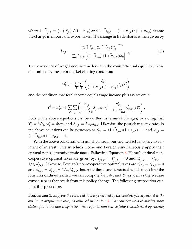
where 1 + tji,k ≡ (1 + t′ji,k)/(1 + tji,k) and 1 + xij,k = (1 + x′ij,k)/(1 + xji,k) denotethe change in import and export taxes. The change in trade shares is then given by

λji,k =

[( 1 + tji,k)( 1 + xji,k)wj

]−εk

∑n λni,k

[( 1 + tni,k)( 1 + xni,k)wn

]−εk. (11)

The new vector of wages and income levels in the counterfactual equilibrium aredetermined by the labor market clearing condition:

w′i Li = ∑k

∑j

(λ′ij,k

(1 + x′ij,k)(1 + t′ij,k)ej,kY′j

)and the condition that total income equals wage income plus tax revenue:

Y′i = w′i Li + ∑k

∑j

(t′ji,k

1 + t′ji,kλ′ji,kei,kY′i +

x′ij,k1 + x′ij,k

λ′ij,kej,kY′j

).

Both of the above equations can be written in terms of changes, by noting thatY′i = YiYi, w′i = wiwi, and λ′ij,k = λij,kλij,k. Likewise, the post-change tax rates in

the above equations can be expresses as t′ji,k = ( 1 + tji,k)(1 + tji,k)− 1 and x′ij,k =

( 1 + xij,k)(1 + xij,k)− 1.With the above background in mind, consider our counterfactual policy exper-

iment of interest: One in which Home and Foreign simultaneously apply theiroptimal non-cooperative trade taxes. Following Equation 6, Home’s optimal non-cooperative optimal taxes are given by: t′f h,k = t∗f h,k = 0 and x′h f ,k = x∗f h,k =

1/εkλ′f f ,k. Likewise, Foreign’s non-cooperative optimal taxes are t′h f ,k = t∗h f ,k = 0and x′f h,k = x∗f h,k = 1/εkλ′hh,k. Inserting these counterfactual tax changes into theformulas outlined earlier, we can compute λij,k, wi, and Yi, as well as the welfareconsequences that result from this policy change. The following proposition out-lines this procedure.

Proposition 1. Suppose the observed data is generated by the baseline gravity model with-out input-output networks, as outlined in Section 3. The consequences of moving fromstatus-quo to the non-cooperative trade equilibrium can be fully characterized by solving

28

the following system of equations

1 + x∗ji,k = 1 + 1εkλii,kλii,k

; 1 + t∗ji,k = 1

λji,k =

[(1+t∗ji,k)(1+x∗ji,k)(1+tji,k)(1+xji,k)

wj

]−εk ˆPεki,k

ˆP−εki,k = ∑j

([(1+t∗ji,k)(1+x∗ji,k)(1+tji,k)(1+xji,k)

wj

]−εk

λji,k

)wiwiLi = ∑k ∑j

[λij,kλij,k

(1+x∗ij,k)(1+t∗ij,k)ej,kYjYj

]YiYi = wiwiLi + ∑k ∑j

(t∗ji,k

1+t∗ji,kλji,kλji,kei,kYiYi +

x∗ij,k1+x∗ij,k

λij,kλij,kej,kYjYj

),

The above system solves N(K + 2) independent unknowns, namely, x∗ji,k, wi, andYi, as a function of industry-level trade elasticities, εk, and the following set of observ-ables: (i) applied trade taxes; (ii) within- and across-industry expenditure shares λji,k,and ei,k; (iii) wage income, wiLi; and (iv) total income, Yi = wiLi +Ri.

Solving the system specified by Proposition 1, determines the welfare conse-quences of dissolving the existing trade agreements as

Value of FTAsi = W−1i =

(Yi

∏kˆPi,k

)−1

.

The consequences of unilateralism can also be measured using a similar approach.To that end, the system specified by Proposition 1 should be modified so that taxesin one country are assigned their unilaterally optimal rate, whereas taxes in therest of the world are assigned their applied rate.

Importantly, the aforementioned procedure is implementable without appeal-ing to any global optimization routine or without knowledge of structural param-eters like τij,k, ai,k, or χij,k. To put our approach in perspective, compare it to thestandard approach that involves a constrained global optimization subject to equi-librium constraints (Costinot and Rodríguez-Clare (2014); Ossa (2014)). The stan-dard approach can be implemented using a nested fixed-point procedure, whichis impractical with many industries (i.e., a high K). Or, alternatively, it can beimplemented using the MPEC procedure in Su and Judd (2012), which requiresspecialized commercial solvers like SNOPT or KNITRO to attain credible results.The procedure outlined by Proposition 1 bypasses these challenges by reducing

29

the global optimization problem to a system of equations that is straightforwardto solve.

Main Model with Input-Output Networks. Now, consider the multi-industrygravity model with input-output networks as presented in Section 4.1. In this ex-tended model, preferences are still characterized by Equation 10; but the price ofgood ij, k depends on the entire vector of industry-level price indexes in country i:

pij,k = (1 + tij,k)(1 + xij,k)τij,kai,kwαi,ki ∏

gP

αi,gki,g .

The change in expenditure shares in response to a change in trade taxes can be,accordingly, specified as

λij,k =

[( 1 + tij,k)( 1 + xij,k)w

αi,ki ∏g

ˆPαi,gki,g

]−εk

∑n λnj,k

[( 1 + tnj,k)( 1 + xnj,k)w

αn,kn ∏g

ˆPαn,gkn,g

]−εk,

where the change in price indexes are given by

ˆP−εki,k = ∑

j

[ 1 + tni,k)( 1 + xni,k)wαn,kn ∏

g

ˆPαn,gkn,g

]−εk

λji,k

.

In the counterfactual equilibrium that arises after the tax change, gross industry-level revenues can be calculated as the sum of sales net of taxes:

Y ′i,k = ∑j

(λ′ij,g

(1 + x′ij,g)(1 + t′ij,g)E′j,k

),

where E′i,k ≡ ei,kY′i + ∑g αi,gkY ′i,g denotes gross expenditure on industry k in coun-try i. Net consumption income is equal to wage income plus tax revenues:

Y′i = w′i Li + ∑k

∑j

(t′ji,k

1 + t′ji,kλ′ji,kE′i,k +

x′ij,k1 + x′ij,k

λ′ij,kE′j,k

).

Wages income in the above expression is itself equal to the sum of labor com-pensation across all industries: w′i Li = ∑k αi,kY ′i,k. As before we can write the

30

above equilibrium conditions in changes by noting that λ′ji,k = λji,kλji,k, w′i = wiwi,Y ′i,k = Yi,kY i,k, and Y′i = YiYi.

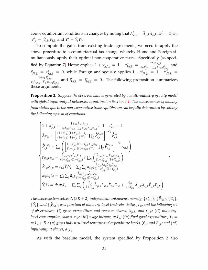
To compute the gains from existing trade agreements, we need to apply theabove procedure to a counterfactual tax change whereby Home and Foreign si-multaneously apply their optimal non-cooperative taxes. Specifically (as speci-

fied by Equation 7) Home applies 1 + x′h f ,k = 1 + x∗h f ,k =1+εkλ′f f ,k

εkλ′f f ,k−∑g α f ,kgr′f h,gand

t′f h,k = t∗f h,k = 0, while Foreign analogously applies 1 + x′f h,k = 1 + x∗f h,k =1+εkλ′hh,k

εkλ′hh,k−∑g αh,kgr′h f ,gand t′h f ,k = t∗h f ,k = 0. The following proposition summarizes

these arguments.

Proposition 2. Suppose the observed data is generated by a multi-industry gravity modelwith global input-output networks, as outlined in Section 4.1. The consequences of movingfrom status-quo to the non-cooperative trade equilibrium can be fully determined by solvingthe following system of equations

1 + x∗ji,k =1+εkλii,kλii,k

εkλii,kλii,k−∑g αj,kg rij,grij,g; 1 + t∗ji,k = 1

λji,k =

[(1+t∗ji,k)(1+x∗ji,k)(1+tji,k)(1+xji,k)

wαi,kj ∏g

ˆPαi,gki,g

]−εk ˆPεki,k

ˆP−εki,k = ∑j

([(1+t∗ji,k)(1+x∗ji,k)(1+tji,k)(1+xji,k)

wαi,kj ∏g

ˆPαi,gki,g

]−εk

λji,k

)rji,krji,k =

λji,kλji,k Ei,kEi,k(1+x∗ji,k)(1+t∗ji,k)

/ ∑n

(λjn,kλjn,k En,gEn,g

(1+x∗jn,k)(1+t∗jn,k)

)Ei,kEi,k = ei,kYiYi + ∑g ∑j αi,gk

λij,gλij,gYj,gYj,g(1+x∗ij,g)(1+t∗ij,g)

wiwiLi = ∑k ∑j αi,kλij,kλij,kYj,kYj,k(1+x∗ij,k)(1+t∗ij,k)

YiYi = wiwiLi + ∑k ∑j

(t∗ji,k

1+t∗ji,kλji,kλji,kEi,kEi,k +

x∗ij,k1+x∗ij,k

λij,kλij,kEj,kEj,k

)

,

The above system solves N(3K+ 2) independent unknowns, namely, x∗ji,k, ˆPi,k, wi,

Yi, and Yi,k, as a function of industry-level trade elasticities, εk, and the following setof observables: (i) gross expenditure and revenue shares, λji,k, and rij,k; (ii) industry-level consumption shares, ei,k; (iii) wage income, wiLi; (iv) final good expenditure, Yi =

wiLi +Ri; (v) gross industry-level revenue and expenditure levels, Yi,k and Ei,k; and (vi)input-output shares, αi,kg.

As with the baseline model, the system specified by Proposition 2 also

31

determines the gains from trade agreements, which are given by W−1i =(

Yi/ ∏kˆPi,k

)−1. Finally, an amended version of Proposition 2 where taxes in one

country are assigned their unilaterally optimal rate, whereas taxes in the rest of theworld are assigned their applied rate, can determine the consequences of unilater-alism.

6.2 Data Description

Our main data source is the 2014 edition of the World Input-Output Database(WIOD, Timmer et al. 2012). The WIOD database covers 56 industries and 42 coun-tries that account for more than 85% of world GDP, plus an aggregate of the restof the world. The countries in the sample include all 27 members of the EuropeanUnion (EU) and 15 other major economies: Australia, Brazil, Canada, China, In-dia, Indonesia, Japan, Mexico, Norway, Russia, South Korea, Switzerland, Taiwan,Turkey, and the United States—see Table 4 in the appendix for a full list of coun-tries. Following Costinot and Rodríguez-Clare (2014), we aggregate the original 56industries in the WIOD into 16 industrial categories, which are listed in Table 1. Fi-nally, we make the WIOD database consistent with our theoretical model by purg-ing it from trade imbalances. In this process, we closely follow the methodologyin Costinot and Rodríguez-Clare (2014) who apply Dekle et al.’s (2007) hat-algebramethodology to purge the 2008 edition of the WIOD.21

We take data on applied tariffs, tji,k, from the United Nations Statistical Divi-sion, Trade Analysis and Information System (UNCTAD-TRAINS). The 2014 ver-sion of the UNCTAD-TRAINS reports the simple tariff line average of the effectivelyapplied tariff (AHS) across 31 two-digit (in ISIC rev.3) sectors, 185 importers, and243 export partners. When tariff data are missing in a given year, we use tariff datafor the nearest available year, giving priority to earlier years. We aggregate theUNCTAD-TRAINS data into individual WIOD industries, following the method-ology in Kucheryavyy et al. (2016). Since individual EU member countries arenot represented in the UNCTAD-TRAINS data during the 2000-2014 period, ouranalysis treats the 27 EU members as one taxing authority.

To map our model to the WIOD and UNCTAD-TRAINS datasets, we treat good

21A similar approach is also applied by Ossa (2014) to eliminate trade imbalances from the GTAPdatabase.

32

ij, k as a good pertaining to WIOD industry k that is supplied by country i to marketj. Under this interpretation, our data reports the following information:

i. The gross expenditure on good ij, k: pij,kqij,k

ii. The applied import tax on good ij, k: tij,k

iii. The share of industry k inputs used in industry g’s output in country i: αi,kg.

Using the above data points, we can construct the within-industry gross expendi-ture shares as

λij,k =pij,kqij,k

∑n pin,kqin,k.

Similarly and assuming xij,k = 0, the within-industry gross output shares can beconstructed as

rij,k =pij,kqij,k/(1 + tij,k)

∑n pin,kqin,k/(1 + tij,k).

The total gross output of industry k in country i can be calculated as the sum ofgross sales net of taxes:

Yi,k = ∑n

[pin,kqin,k/(1 + tij,k)

],

With information on gross output, country i’s net spending on final goods can becalculated as the gross minus intermediate input expenditure:

Yi = ∑j

∑k

(pji,kqji,k

)−∑

k∑g

(αi,kgYi,g

).

The industry-level consumption shares are, accordingly, given by

ei,k =

[∑

j

(pji,kqji,k

)−∑

g

(αi,kgYi,g

)]/Yi.

Finally, wage income can be calculated as the sum of labor compensation across allindustries: wiLi = ∑ αi,kYi,k, where αi,k = 1−∑g αi,gk.22

22To be clear, when applying the above data points to Propositions 1 and 2, we need to assignone country as Home and aggregate the remaining countries into the rest of world.

33

Estimating the Industry-Level Trade Elasticities We estimate the industry-leveltrade elasticities using the triple-difference estimator developed by Caliendo andParro (2014). To present this procedure, note that the multi-industry gravity model(with or without input-output networks) predicts the following formulation fortrade shares:

λij,k = Φi,kΩj,kτ−εkij,k (1 + tij,k)

−εk ,

where Φi,k ≡ a−εki,k w−αi,kεk

i,k ∏g P−αi,gkεki,g and Ωj,k ≡ ∑n

[τ−εknj,k (1 + tnj,k)

−εk Φn,k

]can

be viewed as exporter×industry and importer×industry fixed effects. Suppose theiceberg trade cost, ln τij,k = ln dij,k + εij,k, is composed of two components: (i) asystematic and symmetric component, dij,k = dji,k, that accounts for the effect ofdistance, common language, and common border, and (ii) a random disturbanceterm, ε ji,k, that represents deviation from symmetry. Using this decomposition, wecan produce the following estimating equation for any triplet (j, i, n):

lnλji,kλin,kλnj,k

λij,kλni,kλjn,k= −εk ln

(1 + tji,k)(1 + tin,k)(1 + tnj,k)

(1 + tij,k)(1 + tni,k)(1 + tjn,k)+ ε jin,k,

where ε jin,k ≡ εk(εij,k − ε ji,k + εin,k − εni,k + εnj,k − ε jn,k). Using the above estimat-ing equation, we can attain unbiased and consistent estimates for εk under theidentifying assumption that Corr(tji,k, ε ji,k) = 0. We estimate the above equationseparately for each industry, using data on λji,k from the 2014 version of theWIOD and data on tji,k from the UNCTAD-TRAINS database. The estimationresults are reported in Table 1 and broadly align with those produced by Caliendoand Parro (2014), who use data on a smaller sample of countries from 1993.

6.3 The Consequences of Unilateralism

As an intermediate step we discuss the consequences of unilateralism. For eachcountry, the computed gains from a unilateral adoption of optimal trade taxes arereported in Table 2.23 The same table also reports the externality imposed by thesestaxes on the rest of the world—all in terms of a percentage change in real GDP. The

23Each iteration of our analysis treats one of the countries listed in Table 2 as the Home coun-try and aggregates the remaining countries into one Foreign economy. Alternatively, we can usethe multilateral formulas presented in Section 4.2 to avoid aggregating other countries into oneForeign economy. Doing so delivers welfare gains that are practically indistinguishable from ourbenchmark results.

34

Table 1: List of industries and estimated trade elasticities.

Number Description εk std. err. Obsv.

1Crop and animal production, hunting

0.93 0.19 12,341Forestry and logging

Fishing and aquaculture2 Mining and Quarrying3 Food, Beverages and Tobacco 0.53 0.13 12,3004 Textiles, Wearing Apparel and Leather 2.71 0.51 12,3415 Wood and Products of Wood and Cork 5.64 0.87 12,183

6Paper and Paper Products

4.65 1.49 12,300Printing and Reproduction of Recorded Media

7 Coke, Refined Petroleum and Nuclear Fuel 13.38 1.94 9,538

8Chemicals and Chemical Products

2.36 0.91 12,300Basic Pharmaceutical Products

9 Rubber and Plastics

1.51 0.89 12,34110 Other Non-Metallic Mineral

11Basic Metals

Fabricated Metal Products

12Computer, Electronic and Optical Products

4.07 1.02 12,341Electrical Equipment

13 Machinery and Equipment n.e.c 5.65 1.34 12,341

14Motor Vehicles, Trailers and Semi-Trailers

2.70 0.45 12,341Other Transport Equipment

15 Furniture; other Manufacturing 2.04 0.59 12,341

16All Service-Related Industries

3.80 0.84 12,341(WIOD Industry No. 23-56)

Note: This table estimates the industry-level trade elasticities using the Caliendo and Parro (2014)methodology. The original WIOD industry classification features 56 industries, which we aggregateinto 16 industrial categories.

first two columns in Table 2 report the gains implied by the baseline gravity modelthat overlooks global production networks. The second two columns report thegains implied by our main model that accounts for global production networks.In both cases, we separately report the consequences of first-best unilateral exporttaxes and second-best unilateral import taxes.

35

The numbers reported in Table 2 indicate that for a non-cooperative coun-try first-best export taxes deliver welfare gains that are (on average) 50% largerthan second-best import taxes. On the flip side, non-cooperative export taxesalso inflict a greater negative externality on the rest of the world. This observa-tion speaks to the weight of terms-of-trade versus political economy considerationsin the governments’ objective function. Analyzing import taxes in isolation im-plies a greater role for terms-of-trade considerations (as estimated by Goldberg andMaggi (1999)).24 But in that case, our findings indicate that governments shouldbe applying export taxes more vigorously as they deliver sizable terms-of-tradegains and are not prohibited by the WTO. That export taxes are underexploitedimplies that export-oriented industries have a greater-than-previously-estimated po-litical weight in the governments objective function.

Second-best non-cooperative import taxes are only modestly more effective atmimicking export taxes in the presence of global production networks. As arguedearlier, this outcome is an artifact of an innate tension between two welfare con-siderations: (a) to maintain allocative efficiency in the domestic economy, non-cooperative governments should not tax highly-differentiated intermediate inputs,but (ii) to exploit export market power with second-best import taxes, govern-ments should levy taxes on highly-differentiated intermediate imports. This ten-sion renders import taxes as an ineffective second-best substitute for export taxes.

Global production networks multiply the gains from non-cooperative taxationand the externality of such policies on the rest of the world by 50%. Intuitively,in the presence of global production networks, the excess burden per dollar of taxrevenue falls relatively more on the rest of the world. Consider, for instance, an ex-port tax on rare earth minerals that are used as an input in smartphone productionabroad. A fraction of this export tax is borne on transactions involving foreign pro-ducers and foreign consumers of smartphones. So, through the global productionnetwork, the tax-imposing country can effectively raise revenue on transactionsoccurring outside its jurisdiction—i.e., global production networks present gov-ernments with extra-territorial taxing power.

24To elaborate, Goldberg and Maggi (1999) study the cross-industry variation in import taxesand find that “the weight of welfare in the government’s objective function is many times larger than theweight of contributions.”

36

Table 2: The Welfare Consequences of Unilateralism (% change in real GDP)Baseline Model Model with IO Networks

Export taxation Import taxation Export taxation Import taxationCountry %∆Wi %∆W−i %∆Wi %∆W−i %∆W−i %∆Wi %∆Wi %∆W−i

AUS 1.7% -0.1% 1.3% -0.0% 3.3% -0.1% 2.2% -0.1%EU 0.7% -0.4% 0.5% -0.3% 1.3% -0.8% 1.0% -0.6%BRA 1.2% -0.1% 0.9% -0.0% 2.1% -0.1% 1.4% -0.1%CAN 1.9% -0.1% 1.2% -0.1% 3.6% -0.2% 2.3% -0.1%CHE 1.5% -0.0% 1.2% -0.0% 3.0% -0.1% 2.2% -0.0%CHN 0.5% -0.3% 0.4% -0.2% 1.6% -0.5% 1.4% -0.4%IDN 1.9% -0.0% 1.3% -0.0% 3.7% -0.1% 2.3% -0.0%IND 0.8% -0.0% 0.4% -0.0% 1.6% -0.1% 0.9% -0.1%JPN 0.7% -0.1% 0.5% -0.1% 1.4% -0.2% 1.1% -0.1%KOR 1.2% -0.1% 0.9% -0.0% 3.0% -0.1% 2.4% -0.1%MEX 1.7% -0.0% 1.1% -0.0% 3.0% -0.1% 0.9% -0.0%NOR 3.0% -0.0% 2.3% -0.0% 5.2% -0.1% 3.3% -0.0%RUS 1.6% -0.1% 1.0% -0.0% 3.2% -0.2% 1.9% -0.1%TUR 1.6% -0.0% 1.1% -0.0% 3.4% -0.1% 1.8% -0.0%TWN 1.7% -0.0% 1.3% -0.0% 3.8% -0.1% 3.1% -0.0%USA 0.6% -0.3% 0.4% -0.2% 0.9% -0.5% 0.6% -0.4%Average 1.39% -0.10% 0.99% -0.07% 2.75% -0.19% 1.80% -0.14%

Note: This paper reports the change in a country’s welfare from applying its optimal trade taxes.The baseline model is the perfectly competitive multi-industry gravity model ‘a la Costinot et al.(2011). The model with IO networks is the perfectly competitive multi-industry gravity modelwith input-output networks ‘a la Caliendo and Parro (2014).The gains from unilateral export tax-ation are solved using an amended version of Propositions 1 and 2, where one country acts non-cooperatively and the rest of the world retains their applied tax rates. The gains from (second-best)import taxes concern a scenario where export taxes are inapplicable.

6.3.1 Have Global Production Networks Reduced Protectionist Motives?

Global production networks influence the consequences of unilateralism (a) bychanging the non-cooperative tax level in each country, and (b) by multiplyingwelfare consequences conditional on the chosen tax level. The latter channel is rel-atively well understood and echos the results from the standard gains from tradeliterature. The former channel is new and merits further elaboration. In fact, asnoted in the introduction, some experts argue that existing trade agreements areobsolete because countries that are immersed in global production networks havelittle (terms-of-trade-driven) incentive to raise trade restrictions.

37

Figure 1 illustrates the optimal non-cooperative trade tax schedule for the Eu-ropean Union (E.U.). These are the non-cooperative E.U. taxes given the vector ofapplied taxes by trading partners. As implied by Theorem 1, the optimal exporttax is lower once we account for input-output networks. The intuition is that ex-port taxes cascade through the input-output network, and a fraction of the tax isultimately passed back to domestic consumers. The optimal export tax is set lowerto mitigate these adverse cascading effects. This reduction is especially meaningfulin more upstream industries like Metal, Mining, and Services.

Figure 1: The European Union’s Optimal Non-Cooperative Trade Taxes

Note: This graph plots the optimal trade tax for the E.U. economy against the rest of the world.Industries are ordered by the trade elasticity estimates reported in Table 1. The left panel reportsthe first-best export taxes, normalizing the redundant import taxes to zero. The hollow squarescorrespond to the optimal export taxes predicted by the multi-industry competitive gravity modelwithout input-output networks. Second best import taxes correspond to a scenario where exporttaxes are prohibited.

Second-best non-cooperative import taxes are uniform if we do not account forinput-output networks. Otherwise, they vary across industries in a way that par-tially resembles the optimal first-best export taxes. In particular, the optimal im-port tax is higher on low trade elasticity industries. But, unlike first-best export

38

taxes, it is also relatively higher on upstream industries. The optimal import taxis, for example, higher on Mining and Service industries that are both relativelymore upstream and have a relatively low trade elasticity. The Petroleum industry,in comparison, is relatively upstream but exhibits the highest trade elasticity of allindustries. As a result, the second-best import tax on the Petroleum industry islower than others.25

Importantly, these patterns can reconcile the terms-of-trade thesis with ev-idence that governments assign a low political weight to protecting upstreamindustries because consumers of intermediate inputs are more organized (seeShapiro (2019)). To see this, note that applied tariffs -in absence of externalrestrictions- convey information about the sum of political economy and terms-of-trade considerations (Grossman and Helpman (1992)). Correspondingly, the polit-ical weight of industry-level protection can be inferred as the wedge between thesocially optimal tariff and the applied tariff rate in each industry. A high politicalweight, under this approach, indicates more lobbying for protective tariffs a givenindustry.

Suppose we infer political weights from optimal tariffs that do not internalizeglobal production networks. In that case, we will find no systematic relationshipbetween the level of upstreamness and political weights, which defies the conven-tional wisdom.26 However, if we apply our theory that implies a higher optimaltariff on upstream industries, we will infer a low political weight for protection inthese industries, which aligns with the aforementioned evidence in Shapiro (2019).

Above all, Figure 1 indicates that the globalization of production networks

25The fact that second-best import taxes vary modestly across industries reflects a tension be-tween misallocation-worsening and terms-of-trade-improving effects. To explain this tension again,consider the extreme case where all imported intermediates are re-exported without processing inthe domestic economy. In that case, the second-best import tax schedule converge to the first-bestexport tax schedule. Because, in this extreme case, neither tax instrument distorts input choices inthe domestic economy. This is far from what happens in reality, though—as is clearly manifestedin Figure 1. In practice, industries like Chemicals and Mining that should be targeted with second-best import taxes are both high-value-added and more upstream. So, disrupting them with taxeswill be quite detrimental to allocative efficiency.

26A notable example undertaking this approach is Ossa (2014). He infers political weightsusing optimal tariffs implied by the multi-industry Krugman (1980) model. Optimal tariffs inthe aforementioned model are determined primarily by the industry-level trade elasticities (seeLashkaripour and Lugovskyy (2019)) . Accordingly, Ossa (2014) estimates political weights that arestrongly increasing in an industry’s trade elasticity but are less dependent on an industry’s level ofupstreamness.

39

has not reduced the governments’ incentive to raise trade restrictions. This out-come is driven by all economies, including the E.U., being effectively small openeconomies in relation to the rest of the world. In that case, E.U. taxes on interme-diate inputs have a negligible (albeit non-zero) effect on prices in the rest of theworld. Consequently, the optimal non-cooperative taxes implied with and with-out global production networks are rather similar and resemble the optimal tax ofa small open economy supplying differentiated products.

6.4 The Value of Trade Agreements

As a final step, we quantify the value of existing trade agreements for the globaleconomy. Recall that the value of these agreements is driven by their ability toremedy non-political trade restrictions that ensue in the non-cooperative Nash equi-librium. The extent of these counterfactual restrictions can be measured using thesystem of equations specified under Propositions 1 and 2.27

Table 3 reports the value of existing trade agreements for each country, andcontrasts it to the value implied by the baseline model that overlooks global pro-duction networks. In all cases, the figures are reported under two different scenar-ios: First, a scenario where countries can freely raise all trade tax instruments, inwhich case agreements remedy the first-best non-cooperative export restrictions.Second, a scenario where countries cannot raise export taxes due to institutionalbarriers like those in the U.S. constitution. In this latter case, agreements remedythe second-best non-cooperative import restrictions.

To put the estimated gains from trade agreements in perspective, the last twocolumns of Table 3 report the overall gains from trade relative to autarky. Thesegains are calculated using the sufficient statistics formulas presented by Costinotand Rodríguez-Clare (2014).

The value of trade agreements, as far as remedying unilateral export restrictionis concerned, is around 3.5% of the real GDP for the average country. This amountsto 30% of the overall gains from trade. In other words, if existing trade agreementsdisintegrate, the average country will lose close to a third of the underlying gainsfrom trade. To put a dollar value on these effects, trade agreements add $2.7 trillion

27See Appendix E for how the system specified by Propositions 1 and 2 extends to an environ-ment with arbitrarily many countries.

40

Table 3: The Gains from Trade Agreements (% change in real GDP)

Gains from RemedyingExport Restrictions

Gains from RemedyingImport Restrictions

Overall GainsFrom Trade

Country Baseline IO Networks Baseline IO Networks Baseline IO Networks

AUS 0.1% 0.7% 0.5% 0.9% 5.7% 0.9%EU 1.1% 2.1% 1.1% 1.2% 3.0% 1.2%BRA 0.2% 0.5% 0.4% 0.4% 2.8% 0.4%CAN 2.7% 4.4% 2.1% 2.7% 10.7% 2.7%CHE 3.3% 5.1% 2.8% 3.5% 11.8% 3.5%CHN 0.9% 2.7% 0.9% 1.3% 1.9% 1.3%IDN 0.5% 1.3% 0.8% 0.9% 4.7% 0.9%IND 3.1% 4.3% 1.9% 1.9% 2.5% 1.9%JPN 3.2% 4.7% 1.9% 1.9% 3.5% 1.9%KOR 5.4% 8.6% 3.0% 3.8% 4.4% 3.8%MEX 2.0% 3.0% 2.0% 2.2% 19.8% 2.2%NOR 0.2% 0.3% 0.4% 0.9% 8.8% 0.9%RUS 1.2% 2.4% 1.4% 2.1% 11.1% 2.1%TUR 2.1% 3.5% 2.0% 2.2% 7.9% 2.2%TWN 6.0% 10.2% 4.4% 5.4% 8.1% 5.4%USA 1.0% 1.8% 1.0% 1.0% 2.9% 1.0%Average 2.06% 3.48% 1.66% 2.01% 6.84% 12.70%

Note: This paper reports the change in a country’s welfare from applying its optimal trade taxes.The baseline model is the perfectly competitive multi-industry gravity model ‘a la Costinot et al.(2011). The model with IO networks is the perfectly competitive multi-industry gravity modelwith input-output networks ‘a la Caliendo and Parro (2014). The value of trade agreements atremedying export taxation are solved using the systems specified by Propositions 1 and 2. Thegains from remedying import taxation concern a scenario where non-cooperative export taxes areinapplicable.

to global GDP , which is equal to the size of France’s economy.The above numbers can be viewed as an upper bound on the value of trade

agreements. As note earlier, governments may be obliged to erect only im-port restriction if existing agreements dissolve. In that case, by remedying non-cooperative import restrictions, existing trade agreements add 2% to the averagecountry’s real GDP (see fourth column in Table 3). Altogether, these effects con-tribute a total of $1.6 trillion to global GDP. This second figure can be viewed as alower bound on the value of existing trade agreements.

Around 41% of the estimated value of trade agreements is driven by their pro-

41

motion of global production networks. This number can be inferred by compar-ing the value implied by the baseline model that overlooks global production net-works and the main model that accommodates them. In other words, existingestimates that overlook global production networks may understate the value oftrade agreements by more than 40%. More importantly, these numbers suggestthat the rise of global production networks has rendered trade agreements morevaluable than ever. This is a crucial observation in a time when the tides haveturned against free trade agreements like the WTO.

7 Concluding Remarks

Our understanding of global trade has improved drastically over the past twodecades; thanks in part to the emergence of tractable quantitative trade modelsthat admit a rich geography of trade costs and global production networks. Sur-prisingly, these canonical models have had little impact on how we think abouttrade policy and trade agreements. To address this gap, we presented a full ana-lytical characterization of optimal non-cooperative trade policy in the aforemen-tioned class of quantitative trade models. We demonstrated that the globalizationof production networks have barely reduced the terms-of-trade-driven incentivesto restrict trade; but it has increased the cost of such restrictions quite remarkably.Accordingly, we measured that a disintegration of existing agreements will erase30% of the total gains from trade.

Our theory presents researchers with a new benchmark to study the politicaleconomy of trade taxation in the age of global production networks. The currentpractice in the literature is to infer political economy motives by contrasting theapplied trade taxes with their socially optimal level. Under this approach, ourgeneral theory of optimal trade policy will enable researchers to credibly estimatethe political weight of protecting upstream versus downstream industries. Like-wise, our theory can shed fresh light on the relative importance of terms-of-tradeversus political economy considerations in the conduct of trade policy. Previous es-timates that focus only on import taxation indicate that political considerations aredwarfed by terms-of-trade considerations. Our theory suggests that accountingfor export taxes may revise this prediction.

On a broader level, our findings highlight an important dilemma facing policy-

42

makers in the current political climate. On one hand, critics argue that trade agree-ments infringe on national sovereignty, and limit governments’ ability to tackledomestic distortions, inequality, and environmental issues. On the other hand, wefind that dissolving existing trade agreements will result in extensive losses fromdisrupting global production networks. Future research can perhaps resolve thisdilemma, at the core of which lies a basic question: Can existing agreements bereformed to maintain international cooperation in trade policies but with less in-fringement on national sovereignty?

ReferencesAlvarez, F. and R. E. Lucas (2007). General equilibrium analysis of the eaton–kortum model

of international trade. Journal of monetary Economics 54(6), 1726–1768.

Amiti, M., S. J. Redding, and D. E. Weinstein (2019). The impact of the 2018 tariffs on pricesand welfare. Journal of Economic Perspectives 33(4), 187–210.

Anderson, J. E. and Y. V. Yotov (2016). Terms of trade and global efficiency effects of freetrade agreements, 1990–2002. Journal of International Economics 99, 279–298.

Bagwell, K. and R. W. Staiger (1999). An economic theory of gatt. American EconomicReview 89(1), 215–248.

Bagwell, K., R. W. Staiger, and A. Yurukoglu (2018). Quantitative analysis of multi-partytariff negotiations. Technical report, National Bureau of Economic Research.

Baier, S. L. and J. H. Bergstrand (2007). Do free trade agreements actually increase mem-bers’ international trade? Journal of international Economics 71(1), 72–95.

Baqaee, D. and E. Farhi (2019). Networks, barriers, and trade. Technical report, NationalBureau of Economic Research.

Blanchard, E. J., C. P. Bown, and R. C. Johnson (2016). Global supply chains and tradepolicy. Technical report, National Bureau of Economic Research.

Bown, C., P. Conconi, A. Erbahar, and L. Trimarchi (2020). Trade protection along supplychains.

Caliendo, L., R. C. Feenstra, J. Romalis, and A. M. Taylor (2015). Tariff reductions, entry,and welfare: Theory and evidence for the last two decades. Technical report, NationalBureau of Economic Research.

43

Caliendo, L. and F. Parro (2014). Estimates of the trade and welfare effects of nafta. TheReview of Economic Studies, rdu035.

Carballo, J., K. Handley, and N. Limão (2018). Economic and policy uncertainty: Exportdynamics and the value of agreements. Technical report, National Bureau of EconomicResearch.

Costinot, A., D. Donaldson, and I. Komunjer (2011). What goods do countries trade? aquantitative exploration of ricardo’s ideas. The Review of economic studies, rdr033.

Costinot, A., D. Donaldson, J. Vogel, and I. Werning (2015). Comparative advantage andoptimal trade policy. The Quarterly Journal of Economics 130(2), 659–702.

Costinot, A. and A. Rodríguez-Clare (2014). Trade theory with numbers: Quantifying theconsequences of globalization. In Handbook of international economics, Volume 4, pp. 197–261. Elsevier.

Costinot, A. and I. Werning (2019). Lerner symmetry: A modern treatment. AmericanEconomic Review: Insights 1(1), 13–26.

Das, S. P. (1983). Optimum tariffs on final and intermediate goods. International EconomicReview, 493–508.

Dekle, R., J. Eaton, and S. Kortum (2007). Unbalanced trade. American Economic Re-view 97(2), 351–355.

Egger, P., M. Larch, K. E. Staub, and R. Winkelmann (2011). The trade effects of endogenouspreferential trade agreements. American Economic Journal: Economic Policy 3(3), 113–43.

Fajgelbaum, P. D., P. K. Goldberg, P. J. Kennedy, and A. K. Khandelwal (2020). The returnto protectionism. The Quarterly Journal of Economics 135(1), 1–55.

Goldberg, P. K. and G. Maggi (1999). Protection for sale: An empirical investigation. Amer-ican Economic Review 89(5), 1135–1155.

Grant, M. (2019). Why special economic zones? using trade policy to discriminate acrossimporters.

Gros, D. (1987). A note on the optimal tariff, retaliation and the welfare loss from tariffwars in a framework with intra-industry trade. Journal of international Economics 23(3),357–367.

Grossman, G. M. and E. Helpman (1992). Protection for sale. Technical report, NationalBureau of Economic Research.

Grossman, G. M. and E. Helpman (1995). Trade wars and trade talks. Journal of politicalEconomy 103(4), 675–708.

Irwin, D. A. (2020). Free trade under fire. Princeton University Press.

44

Krugman, P. (1980). Scale economies, product differentiation, and the pattern of trade. TheAmerican Economic Review 70(5), 950–959.

Kucheryavyy, K., G. Lyn, and A. Rodríguez-Clare (2016). Grounded by gravity: A well-behaved trade model with industry-level economies of scale. Technical report, NationalBureau of Economic Research.

Lashkaripour, A. and V. Lugovskyy (2019). Profits, scale economies, and the gains fromtrade and industrial policy.

Limão, N. (2016). Preferential trade agreements. In Handbook of commercial policy, Volume 1,pp. 279–367. Elsevier.

Maggi, G. and A. Rodriguez-Clare (1998). The value of trade agreements in the presenceof political pressures. Journal of Political Economy 106(3), 574–601.

Opp, M. M. (2010). Tariff wars in the ricardian model with a continuum of goods. Journalof International Economics 80(2), 212–225.

Ossa, R. (2014). Trade wars and trade talks with data. The American Economic Re-view 104(12), 4104–4146.

Ossa, R. (2016). Quantitative models of commercial policy. Handbook of Commercial Policy 1,207–259.

Piketty, T. and E. Saez (2013). Optimal labor income taxation. In Handbook of public eco-nomics, Volume 5, pp. 391–474. Elsevier.

Powell, A. A. and F. Gruen (1968). The constant elasticity of transformation productionfrontier and linear supply system. International Economic Review 9(3), 315–328.

Shapiro, J. S. (2019). The environmental bias of trade policy. UC Berkeley and NBER (Ed.),1–76.

Su, C.-L. and K. L. Judd (2012). Constrained optimization approaches to estimation ofstructural models. Econometrica 80(5), 2213–2230.

Suzuki, K. (1978). The welfare effects of an export tax levied on an intermediate good. TheQuarterly Journal of Economics, 55–69.

Timmer, M., A. A. Erumban, R. Gouma, B. Los, U. Temurshoev, G. J. de Vries, I.-a. Arto,V. A. A. Genty, F. Neuwahl, J. Francois, et al. (2012). The world input-output database(wiod): contents, sources and methods. Technical report, Institue for International andDevelopment Economics.

45

Online Appendix

A Proof of Lemma 1

The proof of Lemma 1 follows from two intermediate claims, labeled C1and C2. Topresent these claims, note that A = (1 + t, 1 + x, wh, w f ) and A′ = (a(1 + t), (1 +

x)/a, awh, w f ) . Accordingly, all equilibrium variables corresponding to the wage-taxcombination A′ will be denoted by the prime notation. Claim C1 is based on the demandfunction Dji,k (pi, Yi) being homogeneous of degree zero. Specifically,p′h = aph, Y′h = aYh

p′f = p f , Y′f = aYf

=⇒ q′ji,k = qji,k ∀ji, k. (C1)

where recall that pi ≡ pji,kj,k denotes the vector of final prices in country i. Claim C2can be stated as follows

q′ji,k = qji,k ∀ji, k =⇒

p′h = aph, Y′h = aYh

p′f = p f , Y′f = aYf

. (C2)

The claim that p′h = aph and p′f = p f follow trivially from the price equation:

pji,k = (1 + xji,k)(1 + tji,k)Cj,k(wj, pj; ∑n

τjn,kqjn,k),

given that Ci,k is homogeneous of degree 1 w.r.t. wj and pj. That Y′f = w′f L f = w f L f = Yf ,holds by construction. The claim that Y′h = aYh, meanwhile, can be shown along thefollowing steps:

Y′h = w′hL′h + ∑k

[t′k

1 + t′kp′f h,kq′f h,k +

x′k1 + x′k

p′h f ,kq′h f ,k

]= awhLh + ∑

k

[(1− a

1 + t′k

)p′ f h,kq f h,k +

[a− 1

1 + x′k

]ph f ,kqh f ,k

]awhLh + ∑

k

[(1− a

a(1 + tk)

)ap f h,kq f h,k +

[a− 1

(1 + xk)/a

]ph f ,kqh f ,k

]= awiLi + a ∑

k

[tk

1 + tkp f h,kq f h,k +

xk1 + xk

ph f ,kqh f ,k

]= a (whLh +Rh) ,

46

where the second line follows from the balanced trade condition, i.e.,

∑k

[p f h,kq f h,k

1+tk− ph f ,kqh f ,k

]= 0. Together, Claims C1 and C2 establish Lemma 1.

B Proof of Theorem 1

Note that by definition 1 + tk ≡ p f h,k/p f h,k and 1 + xk ≡ ph f ,k/ph f ,k. Hence, the optimalpolicy problem can be reformulated as a problem of directly choosing consumer prices,p f h,k, and, ph f ,k, rather than taxes, tk, and, xk. In that case, the optimal policy problem canalternatively be expressed as

max(p;w)∈A

Wh (p; w) ,

where A denotes the set of feasible wage-price combinations that is defined analogousto D2. Note that in the presence of input-output linkages, equilibrium is conventionallydefined in terms three sets of equilibrium outcomes: (a) wages, w, (b) net income Y , and(c) gross revenue, Y . However, combining equilibrium conditions (iv) and (v) in D2,we can uniquely solve Y ≡ Y(p; w) and Y ≡ Y(p; w) in terms of prices and wages.Considering this we can uniquely solve all equilibrium variables, including welfare, interms of prices and wages.

To handle the complex nature of the above problem, we use two technical tricks. First,we assume that the government can choose phh in addition to p f h and ph f . In that case,Home’s tax revenues include revenue’s from domestic taxation, which we denote by

RDh ≡∑

k( phh,k − phh,k)qhh,k.

Including the aforementioned instrument is innocuous since (i) markets are perfectlycompetitive, and (ii) governments have not political economy motives for intra-nationalredistribution. As a result, there is no rationale for domestic taxation (i.e., p∗hh,k = phh,k)and the problem with extended instruments becomes isomorphic to our main problemof interest. The second trick that greatly simplifies our analysis is the observation thatdWh(p, w)/dp f f ,k = 0. In light of the above result, we are simply solving a problemwhere the government can directly choose all price variables that matter for Home’s wel-fare. So, we should not track how a change in, say price variable p f h,k, affects any otherconsumer price variables.

Before proceeding to the first step of the proof, let us alert the readers of a slightchange in notation, which is meant to streamline the presentation: We, hereafter, useph f ,k ≡ ph f ,k/(1 + th f ,k) to denote the consumer price of good h f , k net of Foreign’s im-

47

port taxes, and p f h,k ≡ (1+ x f h,k)p f h,k to denote the producer price of good f h, k inclusiveof Foreign’s export taxes.

Step 1: Characterizing the F.O.C. w.r.t. Import Taxes. The F.O.C. with respect to sectork’s tariff can be expressed as

dWh (p; w)

d ln p f h,k=

∂Vh(.)∂Yh

[∂Yh

∂ ln p f h,k+

∂Yh∂wh

dwhd ln p f h,k

]+

∂Vh(.)∂ p f h,k

It should be noted upfront that the difference between the present setup and the pureRicardian case, is that the (conditional) tariff pass-through σ

f h,kjh,g = ∂ ln pjh,g/∂ ln (1 + tk)

can be non-zero (even if g , k) due to (i) the upward sloping supply curve in industryg, plus (ii) the cross-substitutability between industry k and industry g goods. PluggingYh = whLh + Πh +RX

h +RMh +RD

h , into the F.O.C. yields the following:

dWh (p; w)

d ln p f h,k=

∂Vh∂Yh

∂Πh

∂ ln p f h,k+

∂RXh

∂ ln p f h,k+

∂RMh

∂ ln p f h,k+

∂RDh

∂ ln p f h,k

+∂Vh/∂ p f h,k

∂Vh/∂Yh+

∂Vh/∂wh∂Vh/∂Yh

dwhd ln p f h,k

= 0,

where ∂Vh/∂wh = ∂Yh/∂wh + ∑g(∂Vh/∂ pjh,g

) (∂ pjh,g/∂wh

). The above F.O.C. is charac-

terized by six different elements that can be characterized as follows. First, The effect oftariffs on producer surplus, ∂Πh/∂ ln p f h,k, can be expressed as

∂Πh (p; w)

∂ ln p f h,k= ∑

g∑

i=h, f

(∂Πh

∂ ln phi,g

[∂ ln phi,g

∂ ln pIf h,k+

∂phi,g

∂ ln qhh,g

∂ ln qhh,g

∂ ln p f h,k

])+

∂Πh

∂ ln pIf h,k

= ∑g

∑i=h, f

(phi,gqhi,g

[∂ ln phi,g

∂ ln pIf h,k+

∂phi,g

∂ ln qhh,g

∂ ln qhh,g

∂ ln p f h,k

])− p f h,kqIf h,k,

where the second line follows from Hotelling’s lemma that ∂Πhi,g/∂phi,g = qhi,g and∂Πh/∂ pIf h,k = qIf h,k. Second, noting that dWh/dp f f ,g = 0, the effect of import taxes on

48

import tax revenues,RMh ≡ ∑g( p f h,g − p f h,g)q f h,g, can be expressed as

∂RM (p; w)

∂ ln p f h,k=

∂

∂ ln p f h,k

∑g( p f h,g − p f h,g)q f h,g

= p f h,qq f h,k + ∑g

[( p f h,g − p f h,g)q f h,g

∂ ln q f h,g

∂ ln p f h,k− p f h,gq f h,g

∂ ln p f h,g

∂ ln q f h,g

∂ ln q f h,g

∂ ln p f h,k

],

where ∂ ln q f h,g/∂ ln p f h,k accounts for the overall effect p f h,k on final and intermediateinput demand. More specifically, letting D f h,gs(.) denote the demand for intermediateinput variety f h, g from industry s,

∂ ln q f h,g

∂ ln p f h,k=

qCf h,g

q f h,g

(∂ lnD f h,g(.)

∂ ln p f h,k+

∂ lnD f h,g(.)∂ ln Yh

d ln Yhd ln p f h,k

)

+qIf h,g

q f h,g

(∂ ln D f h,g(.)

∂ ln p f h,k+ ∑

sαh,gs

∂ ln D f h,gs(.)∂ lnYh,s

d lnYh,s

d ln p f h,k

)= ε f h,g + η f h,g

d ln Eh,g

d ln p f h,k

where, αh,gs ≡ qIf h,gs/qIf h,g, and Ei,g ≡ ωCi,gYi + ∑s ωIi,gsYi,s denotes demand-weightedgross expenditure on final plus intermediate inputs fro industry g, with the last line fol-

lowing for the implicit assumption that∂ ln D f h,g(.)

∂ lnYh,k=

∂ lnD f h,g(.)∂ ln Yh

and∂ ln D f h,g(.)

∂ ln p f h,k=

∂ lnD f h,g(.)∂ ln p f h,k

for all s. Third, the effect of import taxes on export tax revenues, RXh ≡ ∑g( ph f ,g −

ph f ,g)qh f ,g, can be expressed as

∂RX (p; w)

∂ ln p f h,k=

∂

∂ ln p f h,k

∑g( ph f ,g − ph f ,g)qh f ,g

= ∑g

[( ph f ,g − ph f ,g)qh f ,gηh f ,g

∂ ln E f ,g

∂ ln p f h,k− ph f ,gqh f ,g

(∂ ln ph f ,g

∂ ln pIf h,k+

∂ ln ph f ,g

∂ ln qhh,g

∂ ln qhh,g

∂ ln p f h,k

)].

Fourth, the effect of import taxes on domestic tax revenues, RDh ≡ ∑g( phh,g − phh,g)qhh,g,

can be expressed as

∂RD (p; w)

∂ ln p f h,k=

∂

∂ ln p f h,k

∑g( phh,g − phh,g)q f h,g

=−∑g

[phh,gqhh,g

(∂ ln phh,g

∂ ln pIf h,k+

∂ ln phh,g

∂ ln qhh,g

∂ ln qhh,g

∂ ln p f h,k

)]

49

where the second line implicitly assumes that by the second welfare theorem, p∗hh,k =

phh,k. Fifth, the effect of taxes on the consumer prices can be simplified using Roy’s iden-tity,

∂Vi/∂ pji,g∂Vi/∂Yi

= −qji,g, as follows

∂Vh/∂ ln p f h,k

∂Vh/∂Yh= − p f h,kqCf h,k.

Finally, the effect of tariffs on wages can be determined by applying the implicit functiontheorem to the balanced trade condition, Dh (p, w) = ∑g

(p f h,gq f h,g − ph f ,gqh f ,g

). Doing

so, implies dwhdp f h,k

= − ∂Dh(.)∂ p f h,k

/ ∂Dh(.)∂wh

. Hence, defining τ ≡(

∂Vh∂wh

/ ∂Vh∂Yh

)/ ∂Dh

∂wh,

∂Vh/∂wh∂Vh/∂Yh

dwhd ln p f h,k

= −τ ∑g

p f h,gq f h,g

∂ ln q f h,g

∂ ln p f h,k+

+ p f h,gq f h,g∂ ln p f h,g

∂ ln qhh,g

∂ ln qhh,g

∂ ln p f h,k− ph f ,gqh f ,gηh f ,g

∂ ln E f

∂ ln p f h,k

Combing the above expression as well as noting that ∂Vh/∂Yh > 0 and qji,k = qIji,k + qCji,k,the F.O.C. can be simplified expressed as follows:

∑g

([p f h,g

p f h,g− (1 + τ)

]p f h,gq f h,g

∂ ln q f h,g

∂ ln p f h,k− (1 + τ)

(∂ ln p f h,g

∂ ln q f h,g

∂ ln q f h,g

∂ ln p f h,k

)p f h,gq f h,g

)

+∑g

[(1− (1 + τ)

ph f ,g

ph f ,g

)ph f ,gqh f ,gηh f ,g

]∂ ln E f ,g

∂ ln p f h,k= 0

Given that 1 + t f h,g ≡p f h,gp f h,g

and 1 + xh f ,g ≡ph f ,gph f ,g

, we can further simplify the above ex-

pression if we divide it by 1 + τ and ∑g,i p f i,gq f i,g:28

∑g

[(1 + t f h,g

1 + τ− 1−

∂ ln p f h,g

∂ ln q f h,g

)∂ ln q f h,g

∂ ln p f h,kr f h,g + ∆(xh)

∂ ln Eh,g

∂ ln p f h,k

]= 0

where ∆(xh) ≡ ∑g

[(1− 1

(1+τ)(1+xh f ,g)

)λh f ,gηh f ,g

]. Since (a) Foreign labor is as-

signed as the numeraire, w f = 1, (b) Foreign does not collect tax revenue, and(c) the share of intermediate inputs in Foreign’s production is invariant to p f h,k,then ∂ ln E f ,g/∂ ln p f h,k = 0. Finally, we can determine ∂ ln p f h,k/∂ ln q f h,k by apply-ing the Implicit Function theorem to p f h,k = τf h,kC f ,k(...; ∑i τf i,kq f i,k), which yields

28Since Foreign does not collect tax revenue, gross expenditure in Foreign, E f , also equals gross outputrevenue.

50

∂ ln p f h,k/∂ ln q f h,k = γ f ,kr f h,k/(1− γ f ,kr f f ,kε f f ,k

). Combining these results reduces the

F.O.C. to

∑g

[(1 + t f h,g

1 + τ− 1−

γ f ,kr f h,k

1− γ f ,kr f f ,kε f f ,k

)∂ ln q f h,g

∂ ln p f h,kr f h,g

]= 0. (12)

Step 2. Characterizing the F.O.C. w.r.t. Export Taxes. The F.O.C. with respect to sectork’s export tax can be stated as

dWh (p; w)

d ln ph f ,k=

∂Vh∂Yh

∂Πh

∂ ln ph f ,k+

∂RXh

∂ ln ph f ,k+

∂RMh

∂ ln ph f ,k+

∂RDh

∂ ln ph f ,k

+∂Vh/∂ ln ph f ,k

∂Vh/∂Yh+

∂Vh/∂wh∂Vh/∂Yh

dwhd ln ph f ,k

= 0,

In the above expression,∂Vh/∂ ln ph f ,k

∂Vh/∂Yh= 0. The remaining non-zero elements can be ex-

pressed as follows. First, The effect of export taxes on producer surplus, ∂Πh/∂ ph f ,k, canbe expressed as

∂Πh (p; w)

∂ ln ph f ,k= ∑

g∑

i=h, f

(∂Πhi,g

∂phi,g

∂phi,g

∂ ln ph f ,k

)+

∂Πh

∂ ln pIh f ,k

= ∑g

∑i=h, f

(phi,gqhi,g

∂phi,g

∂ ln qh f ,g

∂ ln qh f ,g

∂ ln ph f ,k

),

where the last line follows from Hotelling’s lemma that ∂Πhi,g/∂phi,g = qhi,k and∂Πh/∂pIh f ,g = 0. Second, the effect of export taxes on import tax revenues, RM

h ≡∑g( p f h,g − p f h,g)q f h,g, can be expressed as

∂RM (p; w)

∂ ln ph f ,k=

∂

∂ ln ph f ,k

∑g( p f h,g − p f h,g)q f h,g

= −∑g

[( p f h,g − p f h,g)η f h,g

∂ ln Eh∂ ln ph f ,k

+ p f h,gq f h,g∂ ln p f h,g

∂ ln pIh f ,k

]

51

Third, the effect of export taxes on export tax revenues, RXh ≡ ∑g( ph f ,g − ph f ,g)qh f ,g, can

be expressed as

∂RX (p; w)

∂ ln ph f ,k=

∂

∂ ln ph f ,k

∑g( ph f ,g − ph f ,g)qh f ,g

=∑g

[(ph f ,g − ph f ,g

)qh f ,g

∂ ln qh f ,g

∂ ln ph f ,k− ph f ,gqh f ,g

∂ ln ph f ,g

∂ ln qh f ,g

∂ ln qh f ,g

∂ ln ph f ,k

]

Fourth, the effect of import taxes on domestic tax revenues, RXh ≡ ∑g( phh,g − phh,g)qhh,g,

can be expressed as

∂RD (p; w)

∂ ln ph f ,k=

∂

∂ ln ph f ,k

∑g( phh,g − phh,g)q f h,g

=−∑g

[phh,gqhh,g

∂ ln phh,g

∂ ln qh f ,g

∂ ln qh f ,g

∂ ln ph f ,k

]

where the second line implicitly assumes that by the second welfare theorem, p∗hh,k =

phh,k. Finally, the effect of export taxes on wages can be determined by applying the im-plicit function theorem to the balanced trade condition, Dh = ∑g p f h,gq f h,g − ph f ,gqh f ,g.Doing so, implies dwh

dph f ,k= − ∂Dh

∂ ph f ,k/ ∂Dh

∂wh. Hence, adopting our earlier definition, τ ≡(

∂Vh∂wh

/ ∂Vh∂Yh

)/ ∂Dh

∂wh,

∂Vh/∂wh∂Vh/∂Yh

dwhd ln ph f ,k

= −τ

∑g

[p f h,gq f h,g

(∂ ln p f h,g

∂ ln pIh f ,k+ η f h,g

∂ ln Eh∂ ln ph f ,k

)]

− ph f ,kqh f ,k −∑g

ph f ,gqh f ,g∂ ln qh f ,g

∂ ln ph f ,k

Combing the above expression as well as noting that ∂Vh/∂Yh > 0 and qji,k = qIji,k + qCji,k,the F.O.C. can be simplified expressed as follows:

(1 + τ)∑g

(p f h,gq f h,gαh,k

f ,g

)+ ∑

g

([(1 + τ)−

ph f ,g

ph f ,g

]ph f ,gqh f ,g

∂ ln qh f ,g

∂ ln ph f ,k

)

+

(∑g

[p f h,g

p f h,g− (1 + τ)

]p f h,gq f h,gη f h,g

)∂ ln Eh

∂ ln ph f ,k,

52

where recall that∂ ln qh f ,g∂ ln ph f ,k

= εh f ,kh f ,g + ηh f ,g

∂ ln E f∂ ln ph f ,k

. Given that 1+ t f h,g ≡p f h,gp f h,g

and 1+ xh f ,g ≡ph f ,gph f ,g

, we can further simplify the above expression if we divide it by 1 + τ and E f (noting

that p f h,kq f h,k = r f h,kE f and ph f ,gqh f ,g = λh f ,gE f ):

λh f ,k + ∑g

([1− 1

(1 + xh f ,g)(1 + τ)

]λh f ,gε

h f ,kh f ,g

)

−∑g

(r f h,gαh,k

f ,g

) Yf

E f+ ∆h(th)

∂ ln Eh∂ ln ph f ,k

+∆ f (x)∂ ln E f

∂ ln ph f ,k= 0,

where ∆h(th) ≡ ∑g

([1+t f h,g

1+τ − 1]

r f h,gη f h,g

)is a uniform term. As noted before, given our

choice of numeraire, ∂ ln E f /∂ ln ph f ,k = 0. Given the Lerner symmetry and the multiplic-ity of the optimal trade tax, there always exists a solution to the above problem where∆h(t) = 0. Henceforth, we restrict our attention to solving for this particular solution.Once we do that, the remaining solutions can be identified with a basic multiplicativetransformation of the import and export tax vectors. yields the following optimality con-dition:

λh f ,k + ∑g

([1− 1

(1 + xg)(1 + τ)

]λh f ,gε

h f ,kh f ,g

)−∑

g

(r f h,gαh,k

f ,g

)= 0. (13)

Step 3: Simultaneously Solving the System of F.O.C. As a final step, we simultaneouslysolve the system of F.O.C.s for all tax instruments:

∑g

[(1 + tg

1 + τ− 1− γ f h,g

)∂ ln q f h,g

∂ ln p f h,kr f h,g

], ∀k ∈ K

∑g

([1

(1 + xg)(1 + τ)− 1]

λh f ,g

λh f ,kεh f ,g

)= 1−∑

g

r f h,g

λh f ,kα

h f ,kf h,g, ∀k ∈ K

First, note that by the Lerner symmetry, the value of τ is redundant. In other words,replacing 1 + τ with any 1 + t ∈ R+ identifies an optimal tax schedule. To derive a sim-plified expression for optimal export taxes, define Ωh f ,k ≡ 1−∑g

(r f h,gλh f ,k

αh,kf ,g

)and suppose

the optimal export tax has the following formulation:

1 + x∗h f ,k =εh f ,k

εh f ,k + ξh f ,k + Ωh f ,k.

53

Plugging the above expression back into the F.O.C. implies that that

∑g(ξh f ,g + Ωh f ,g

) λh f ,gεh f ,kh f ,g

λh f ,kεh f ,k= Ωh f ,k. This equation can be written in matrix notation

as Ξ (ξ + Ω) = Ω, where ξ ≡ [ξh f ,k]k and Ω ≡ [Ωh f ,k]k are K × 1 vectors and

Ξ ≡ [λh f ,gε

h f ,kh f ,g

λh f ,kεh f ,k]k,g and IK are K× K matrixes. Inverting the above system implies that

[ξh f ,k]k =(

Ξ−1 − IK

)Ω. (14)

So, altogether the following tax schedule corresponds to an optimal policy for an arbitrarychoice of 1 + t ∈ R+:

1 + t∗f h,k =

(1 +

γ f ,kr f h,k

1− γ f ,kr f f ,kε f f ,k

)(1 + t)

1 + x∗h f ,k =εh f ,k

1 + εh f ,k + ξh f ,k −∑gr f h,g

λh f ,kα

h f ,kf h,g

(1 + t)−1,

where ξh f ,k is given by Equation 14.

C Proof of Theorem 2

The F.O.C. with respect to sector k’s tariff can be expressed as

dWh (p; w)

d ln p f h,k=

∂Vh(.)∂Yh

[∂Yh

∂ ln p f h,k+

∂Yh∂wh

dwhd ln p f h,k

]+

∂Vh(.)∂ p f h,k

It should be noted upfront that the difference between the present setup and the pureRicardian case, is that the (conditional) tariff pass-through σ

f h,kjh,g = ∂ ln pjh,g/∂ ln (1 + tk)

can be non-zero (even if g , k) due to (i) the upward sloping supply curve in industryg, plus (ii) the cross-substitutability between industry k and industry g goods. PluggingYh = whLh +RM

h , into the F.O.C. yields the following:

dWh (p; w)

d ln p f h,k=

∂Vh∂Yh

∂RM

h∂ ln p f h,k

+∂Vh/∂ p f h,k

∂Vh/∂Yh+

∂Vh/∂wh∂Vh/∂Yh

dwhd ln p f h,k

= 0,

54

By Roy’s identity

∂Vh/∂ ln p f h,k

∂Vh/∂Yh= − p f h,kqCf h,k −∑

gphh,gqChh,g

∂ ln pChh,g

∂ ln pIf h,k

= − p f h,kqCf h,k −∑g

phh,gqChh,gαf ,kh,g

where αf ,ki,k ≡ ∂ ln pij,g/∂ ln pIf h,k denotes the general equilibrium effect of a change in p f h,k

on the price industry g’s output in country i.29 The K×K matrix for αf ,kf ,k can be calculated

by applying the Implicit Function Theorem to p f i,k = (1 + t f i,k)τf i,kC f ,k(w f , pIf f , pIh f ),which implies that

[α

f ,kf ,g

]k,g

=

(IK −

[α

f ,kf ,g

]k,g

) [αh,k

f ,g

]k,g

[α

f ,kh,g

]k,g

,

Likewise, αf ,kf ,k can be calculated by applying the Implicit Function Theorem to phi,k =

τhi,kCh,k(w f , pIf h, pIhh), which yields the following:

[α

f ,kh,g

]k,g

=

(IK −

[αh,k

h,g

]k,g

) [α

f ,kh,g

]k,g

.

With the above definition in mind, the effect of import taxes on import tax revenues,RM

h ≡ ∑g( p f h,g − p f h,g)q f h,g, can be expressed as

∂RM (p; w)

∂ ln p f h,k=

∂

∂ ln p f h,k

∑g( p f h,g − p f h,g)q f h,g

= p f h,qq f h,k + ∑g

[( p f h,g − p f h,g)q f h,g

(∂ ln q f h,g

∂ ln p f h,k+

∂ ln q f h,g

∂ ln phh,gα

f ,kh,s

)− p f h,gq f h,gα

f ,kf ,s

],

where as before (with a slight abuse of notation)∂ ln q f h,g∂ ln pih,k

=∂ ln q f h,g∂ ln pih,k

+ η f h,g∂ ln Eh,g∂ ln pih,k

. Theincome driven term, however, can be dropped as it has a second-order effect, since

29To keep things simple, we are exercising a slight abuse of notation here. A a more elaborate choice ofnotation would be α

f h,ki,k ≡ ∂ ln pij,g/∂ ln pIf h,k, which clarifies that α

f h,ki,k , α

f f ,ki,k .

55

∂ ln Eh,g∂ ln pih,k

∝ (RMh /Yh)λih,k, where δh ≈ λih,k ≈ 0.

∂Vh/∂wh∂Vh/∂Yh

dwhd ln p f h,k

= −τ ∑g

p f h,gq f h,g

(∂ ln q f h,g

∂ ln p f h,k+

∂ ln q f h,g

∂ ln phh,gα

f ,kh,s

)+

+ p f h,gq f h,gαf ,kf ,g − ph f ,gqh f ,g

∂ ln qh f ,g

∂ ln ph f ,gα

f ,kh,g

Finally, we have to plug Equations back into the F.O.C.. To simplify some terms we canuse the zero profits condition, which entails that

∂Πh (p; w)

∂ ln p f h,k= ∑

g∑

i=h, f

(∂Πh

∂ ln phi,g

∂ ln phi,g

∂ ln pIf h,k

)+

∂Πh

∂ ln pIf h,k+ ∑

g

(∂Πh

∂ ln pIhh,k

∂ ln pIhh,g

∂ ln pIf h,k

)= ∑

g∑

i=h, f

(phi,gqhi,gα

f ,kh.g

)− p f h,kqIf h,k −∑

g

(phh,gqIhh,gα

f ,kh.g

)= 0,

Combining the above expressions, the F.O.C. can be stated as

∑g

([p f h,g

p f h,g− (1 + τ)

] (ε f h,g + ε

hh,gf h,gα

f ,kh,g

)− (1 + τ)α

f ,kf ,g

)p f h,gq f h,g

+∑g

(ph f ,gqh f ,g

[(1 + τ)α

f ,kh,g + τεh f ,gα

f ,kh,g

])= 0

where note that p f h,g/p f h,g = 1 + t f h,k. To further simplify the above expression, we candivide by 1 + τ and gross expenditure in Foreign (which equal gross production revenuesince Foreign collects no tax revenue, i.e., ∑k E f ,k = ∑k Y f ,k), which yields

∑g

([(1 + t f h,g

1 + τ− 1)(

ε f h,g + εhh,gf h,gα

f ,kh,g

)− α

f ,kf ,g

]r f h,g

+

[(1 +

τ

1 + τεh f ,g

)α

f ,kh,g

]λh f ,k

)= 0. (15)

56

The next step is to characterize τ ≡ −∂(W f /∂w f )∂ ∑g(p f h,gq f h,g−ph f ,gqh f ,g)/∂w f

, where the partial derivative

denotes the derivative with respect to w f holding p f h,k fixed.

τ =−∑g p f h,kq f h,g

∂ ln p f h,g∂ ln w f

∑g p f h,gq f h,g∂ ln p f h,g∂ ln w f

− ph f ,gqh f ,g

(∂ ln qh f ,g∂ ln p f f ,g

∂ ln p f f ,k∂ ln w f

+∂ ln qh f ,g∂ ln E f ,g

∂ ln E f ,g∂ ln w f

)=

−∑g p f h,kq f h,g∂ ln p f h,g∂ ln w f

∑g p f h,gq f h,g∂ ln p f h,g∂ ln w f

−∑g ph f ,gqh f ,g(εh f ,g + ηh f ,g

)δ f ,g

=−∑g p f h,kq f h,gδ f ,k

∑g p f h,gq f h,gδ f ,k + ∑g ph f ,gqh f ,gεh f ,kδ f ,k= − 1

1 + ∑g ωh f ,gεh f ,g= − 1

1 + εh f,

where the second line follows from the well-known result in consumer theory that

∑i

(ε

f i,gh f ,g

)+ ηh f ,g = 0; εh f denotes the elasticity of foreign demand for labor as defined

under Definition D5; and ωh f ,g ≡ δ f ,kλh f ,k/ ∑k δ f ,kr f h,k is the weight assigned to industryg when calculating the elasticity of labor demand. δ f ,g, meanwhile, denotes the total con-tribution of Foreign labor to industry-level output. As discussed in Section 3.1, the vectorδ f ≡ [δi,k]k cam be calculated as

δ f =(

IK − α f f)−1

α f ,

where recall that α f≡ [α f ,k]k is a K × 1 vector and α f f ≡ [αf ,kf ,g]k,g is a K × K input-output

matrix. Also, note that if Home is sufficiently small compared to Foreign (which is oftenthe case since Foreign is an aggregate of the rest of the world), then δ f ,k ≈ 1 in which caseωh f ,g ≈ λh f ,g/λh f . Finally, plugging the all the above expressions back into the Equation15, and inverting the system specified by this equation implies that

1 + t∗f h,k =εh f

1 + εh f

(1 +

τkε f h,k

),

where τ ≡ [τk] is given by

τ =

1k=g +ε

hh,gf h,g

ε f h,kα

f ,kh,g

−1

k,g

[∑

g∈K

(α

f ,kf ,g − [1 +

εh f ,g

εh f]λh f ,g

r f h,gα

f ,kh,g

)]k

.

57

D The Multiple Country Case

Suppose there are arbitrarily many countries. Then, the effect of country i’s import tax onown welfare can be expressed as

dWi(.)d ln(1 + tji,k)

=∂Wi(.)

∂ ln(1 + tji,k)+ ∑

,j

∂Wi(.)∂ ln w

d ln w

d ln(1 + tji,k).

It is straightforward to show that ∂Wi(.)∂ ln w

d ln w

d ln(1+tji,k)∝ λiri,kλji,k, and that based on actual

trade data, λiri,k/λiirii,k ≈ 0 for , i. So, treating labor in country j as the numeraire,changes in welfare can be approximated to a first-order as

dWi(.)d ln(1 + tji,k)

≈ ∂Wi(.)∂ ln(1 + tji,k)

+∂Wi(.)∂ ln wi

d ln wi

d ln(1 + tji,k).

The same applies to export taxes. Wee can, thus, cast the Country i’s optimal policy prob-lem as one that maximizes Wi(p, wi) by choosing pij,k and pji,ksubject to feasibilityconstraints. Following the same steps taken in Appendix B, the F.O.C. corresponding toprice pji,k (i.e., import tax, tji,k) can be expressed as:

∑g

∑

[(1 + tji,g

1 + τi− 1− γi,g

)∂ ln qi,g

∂ ln pji,kpi,gqi,g

]= 0.

γji,k can be derived by applying the Implicit Function Theorem to pji,k =

τji,kCi(..., ∑g ∑ι τjι,gqjι,g), which implies the following:

γji,k =γj,krji,k

1−∑ι,i γj,krjι,kε jι,k.

Likewise, the F.O.C. corresponding price pij,k (i.e., export tax, xij,k) can be expressed as:

∑g

∑

[(1 + ti,g

1 + τ− 1− γji,g

)∂ ln qi,g

∂ ln pji,k

pi,gqi,g

pij,gqij,g

], ∀k ∈ K

∑g

([1

(1 + xij,g)(1 + τi)− 1

]λij,g

λij,kεij,g

)= 1−∑

g∑

Λi,g

Λij,kαi,k

j,g, ∀k ∈ K

58

where Λi,g ≡ pji,gqji,g/ ∑,i ∑k pi,kqi,k; Λij,g ≡ pij,gqij,g/ ∑,i ∑k pi,kqi,k; and[αi,k

j,g

]=

αijα

j if , j, with

[αi,k

jj,g

]= αi

j. Combining the above expressions implies

1 + t∗ji,k =

(1 +

γj,krji,k

1−∑ι,i γj,krjι,kε jι,k

)(1 + t)

1 + x∗ij,k =εij,k

1 + εij,k + ξij,k −∑g ∑Λi,g

Λij,kαi,k

j,g

(1 + t)−1.

Uniformity of Import Taxes. Here, we establish the uniformity of import taxes (whenγi,k = 0) without invoking any first-order approximation. Analogous to the two-countrymodel, welfare in country i can be expressed as Wi = ∂Vi (Yi, pi), where Yi = wiLi +

∑k(tji,k pji,kqji,k + xij,k pij,kqij,k

). Correspondingly, Wi is uniquely determined by the vector

of import and export taxes, ti = tji,k and xi = xij,k, plus the vector of country-levelwages, w = wj:

Wi (ti, xi; w) = Vi (Yi (ti, xi; w) , pi (ti, xi; w))

Defining Di (ti, xi; w) = wiLi − ∑k ∑` (pi`,kqi`,k), the equilibrium vector of aggregatewages, w, solves the following system of equations:

D1 (t1, x1; w) = 0...

DN (tN, xN; w) = 0

(16)

Keeping the above observation in mind, we can write the F.O.C. with respect to tji,k as

dWi (ti, xi; w)

d(1 + tji,k

) =∂Vi (Yi, pi)

∂Yi

[∂Yi

∂(1 + tji,k

) + ∂Yi

∂wi

dwi

d(1 + tji,k

)]

+ ∑g∈K

∑`∈C

(∂Vi (Yi, pi)

∂ p`i,g

[∂ p`i,g

∂(1 + tji,k

) + ∂ p`i,g

∂w`

dw`

d(1 + tji,k

)])

=∂Vi (Yi, pi)

∂Yi

∂Yi

∂(1 + tji,k

) + ∂Vi (Yi, pi) /∂ pji,k

∂Vi (Yi, pi) /∂Yi

∂ pji,g

∂(1 + tji,k

) + ∑`

(∂Wi (.)

∂w`

dw`

d(1 + tji,k

)) = 0

59

Invoking Roy’s identity,∂Vi(Yi,pi)/∂ pji,k∂Vi(Yi,pi)/∂Yi

= qji,k, and noting that

∂Yi

∂ ln(1 + tji,k

) = pji,kqji,k + ∑`∈C

∑g∈K

[t`i,k p`i,kq`i,k

(ε

ji,k`i,g + η`i,g

∂ ln Yi

∂ ln(1 + tji,k

))]

Plugging the above equation back into the F.O.C. and defining ∆ji,k`i,g ≡ ε

ji,k`i,g +

η`i,g∂ ln Yi

∂ ln(1+tji,k), will yield the following optimality condition

dWi (ti, xi; w)

d ln(1 + tji,k

) =∂Vi (Yi, pi)

∂Yi

[pji,kqji,k − pji,kqji,k + ∑

`∈C

∑g∈K

(t`i,k p`i,kq`i,k∆ji,k

`i,g

)− ∑

`∈C

(νi`

d ln w`

d ln(1 + tji,k

))] ,

where νi` ≡ ∂Wi/∂ ln w`. Applying the implicit function theorem to the System of Equa-tions 16, we can solve for d ln w/d ln 1 + ti as follows:

d ln w1d ln(1+t1i,k)

· · · d ln w1∂ ln(1+tNi,k)

... . . . ...d ln wN

d ln(1+t1i,k)· · · d ln wN

d ln(1+tNi,k)

=

(∂ ln D∂ ln w

)−1

∂ ln D1

∂ ln(1+t1i,k)· · · ∂ ln D1

∂ ln(1+tNi,k)... . . . ...

∂ ln DN∂ ln(1+t1i,k)

· · · ∂ ln DN∂ ln(1+tNi,k)

,

Letting τ`i denotes element `i of matrix (∂ ln D/∂ ln w)−1, the above system implies thatfor every ` ∈ C

d ln w`

d ln(1 + tji,k

) = ∑`∈C

(τ`n ∑

g∈K

(pni,gqni,g∆ji,k

ni,g

)).

Plugging the above expression back into the F.O.C. implies the following

∑n∈C

∑g∈K

(tni,g pni,gqni,g∆ji,k

ni,g

)− ∑

`∈C

(ν` ∑

n∈C

(τ`n ∑

g∈K

pni,gqni,g∆ji,kni,g

))= 0.

The above expression can in turn be rearranged as

∑n∈C

∑g∈K

[(tni,g − ∑

`∈Cτ`nνi`

)pni,gqni,g∆ji,k

ni,g

]= ∑

n∈C

∑g∈K

[(tni,g − τni

)pni,gqni,g∆ji,k

ni,g

]= 0,

60

where τni ≡ ∑`∈C τ`nνi`, or, equivalently

T i∆i = 0,

where T i =[tni,g − τni

]ng∈C×K

and ∆i =[

pni,gqni,g∆ji,kni,g

]ng,jk∈C×K

are respectively 1× N ·K and N · K× N · K matrixes. If det ∆i , 0, then T i = 0 is the unique solution to the abovesystem, which implies that the optimal import tax is uniform across products originatingfrom the same exporting country:

t∗ji,k = τji, ∀j, k.

E Quantitative Implementation with Many Countries

This appendix extends the quantitative procedure outlined in Section 6 to environmentsthat feature arbitrarily many countries.

Baseline Model without IO Networks. Without input-output network (i.e., αi,kj,g = 0)

and with CES-Cobb-Douglas preferences (i.e., εij,k = −1− εk(1− λij,k)), Equation 8 im-plies the an optimal export tax on good ji, k that is equal to

1 + x∗ij,k = 1 +1

εk(1− λij,kλij,k),

where for for each variable, xx denotes the counterfactual value in the non-cooperativeequilibriumCombining the above formula with the equilibrium conditions specified inSection 6 yields the following system of equations:

1 + x∗ij,k = 1 + 1εk(1−λij,kλij,k)

; 1 + t∗ji,k = 1

λji,k =

[(1+t∗ji,k)(1+x∗ji,k)(1+tji,k)(1+xji,k)

wj

]−εk ˆPεki,k

ˆP−εki,k = ∑j

([(1+t∗ji,k)(1+x∗ji,k)(1+tji,k)(1+xji,k)

wj

]−εk

λji,k

)wiwiLi = ∑k ∑j

[λij,kλij,k

(1+x∗ij,k)(1+t∗ij,k)ej,kYjYj

]YiYi = wiwiLi + ∑k ∑j

(t∗ji,k

1+t∗ji,kλji,kλji,kei,kYiYi +

x∗ij,k1+x∗ij,k

λij,kλij,kej,kYjYj

).

61

Solving the above system determines the welfare consequences of dissolving the existingtrade agreement: Wi = Yi/ ∏k

ˆPi,k.

Main Model with IO Networks. Now, consider the main model with input-output net-works. By Equation 8, the optimal export tax on good ji, k can be expressed as

1 + x∗ij,k =1 + εk(1− λij,kλij,k)

εk(1− λij,kλij,k)−∑g ∑ι,iλιj,gλιj,g Ej,gEj,g

(λij,kλij,k Ej,kEj,k)(1+tιj,g)(1+xιj,g)αi,k

j,g

,

where for for each variable, xx denotes the counterfactual value in the non-cooperativeequilibrium; while αi,k

jj,g = λij,kλij,kαj,kg and

[αi,k

j,g

]=[λij,kλij,kαj,kg

]k,g

[λj,gλi,gα,gk

]k,g ,

if , j. Combining the above formula with the equilibrium conditions specified in Ap-pendix 6 yields the following system of equations:

1 + x∗ij,k =1+εk(1−λij,kλij,k)

εk(1−λij,kλij,k)−∑g ∑ι,iλιj,gλιj,gEj,gEj,g

(λij,kλij,k Ej,kEj,k)(1+tιj,g)(1+xιj,g)αi,k

j,g

; 1 + t∗ji,k = 1

λji,k =

[(1+t∗ji,k)(1+x∗ji,k)(1+tji,k)(1+xji,k)

wαi,kj ∏g

ˆPαi,gki,g

]−εk ˆPεki,k

ˆP−εki,k = ∑j

([(1+t∗ji,k)(1+x∗ji,k)(1+tji,k)(1+xji,k)

wαi,kj ∏g

ˆPαi,gki,g

]−εk

λji,k

)rji,krji,k =

λji,kλji,k Ei,kEi,k(1+x∗ji,k)(1+t∗ji,k)

/ ∑n

(λjn,kλjn,k En,gEn,g

(1+x∗jn,k)(1+t∗jn,k)

)Ei,kEi,k = ei,kYiYi + ∑g ∑j αi,gk

λij,gλij,gYj,gYj,g(1+x∗ij,g)(1+t∗ij,g)

wiwiLi = ∑k ∑j αi,kλij,kλij,kYj,kYj,k(1+x∗ij,k)(1+t∗ij,k)

YiYi = wiwiLi + ∑k ∑j

(t∗ji,k

1+t∗ji,kλji,kλji,kEi,kEi,k +

x∗ij,k1+x∗ij,k

λij,kλij,kEj,kEj,k

)

.

Solving the above system determines the welfare consequences of dissolving the existingtrade agreement: Wi = Yi/ ∏k

ˆPi,k

62

Table 4: List of countries in quantitative analysis

Country name WIOD code Basic aggregationAustralia AUS AustraliaBrazil BRA BrazilCanada CAN CanadaChina CHN ChinaIndonesia IDN IndonesiaIndia IND IndiaJapan JPN JapanKorea KOR KoreaMexico MEX MexicoRussia RUS RussiaTurkey TUR TurkeyTaiwan TWN TaiwanUnited States USA United StatesAustria AUT

European Union

Belgium BELBulgaria BGRCyprus CYPCzech Republic CZEGermany DEUDenmark DNKSpain ESPFinland FINFrance FRAUnited Kingdom GBRGreece GRCHungary HUNIreland IRLItaly ITANetherlands NLDPoland POLPortugal PRTRomania ROMSlovakia SVKSlovenia SVNSweden SWEEstonia ESTLatvia LVALithuania LTULuximburg LUXMalta MLTRest of the World RoW Rest of the World

63