the control complexity of sincere-strategy preference
TRANSCRIPT
The Control Complexity ofSincere-Strategy Preference-Based
Approval Voting and of Fallback Voting,and a Study of Optimal Lobbying and
Junta Distributions for SAT
Inaugural-Dissertation
zurErlangung des Doktorgrades der
Mathematisch-Naturwissenschaftlichen Fakultatder Heinrich-Heine-Universitat Dusseldorf
vorgelegt von
Gabor Erdelyiaus Baja
Dusseldorf, im Januar 2009

Aus dem Institut fur Informatik derHeinrich-Heine-Universitat Dusseldorf
Gedruckt mit der Genehmigung derMathematisch-Naturwissenschaftlichen Fakultat derHeinrich-Heine-Universitat Dusseldorf
Referent: Prof. Dr. Jorg Rothe
Koreferent: Prof. Dr. Egon Wanke
Tag der mundlichen Prufung: 16.03.2009

Erkl arung
Hiermit erklare ich, dass ich die vorliegende Dissertation selbstandig und nur unter Ver-wendung der angegebenen Quellen und Hilfsmittel angefertigt habe.
Teile dieser Arbeit wurden bereits in den folgenden Schriften veroffentlicht bzw. zurPublikation angenommen: [EHRS07a, EHRS07b, ENR08a, ENR08b, BEH+ar]. EinigeErgebnisse des Forschungsberichts [EHRS07b] wurden bei der Zeitschrift TheoreticalComputer Scienceunter dem Titel “Generalized Juntas an NP-Hard Sets” und andereErgebnisse von [EHRS07b] wurden bei der ZeitschriftInformation Processing Lettersunter dem Titel “Frequency of Correctness versus Average Polynomial Time” eingereicht.Einige Ergebnisse des Forschungsberichts [ENR08b] wurdenbei der ZeitschriftMathe-matical Logic Quarterlyfur die SonderausgabeLogic and Complexity within Computa-tional Social Choiceunter dem Titel “Sincere-Strategy Prefernce-Based Approval VotingFully Resists Constructive Control and Broadly Resists Destructive Control” eingereicht.
Dusseldorf, 16. Januar 2009 Gabor Erdelyi
iii


Acknowledgments
First of all, I am deeply grateful to my advisor Jorg Rothe for giving me the chance tojoin his research team. Without his support, help, and inspiring discussions I would neverhave had the chance to gain ground in the scientific community.
Moreover, I would like to thank Egon Wanke for serving as a referee for this thesis.I further thank all my coauthors, including Dorothea Baumeister, Dagmar Bruß, Edith
Hemaspaandra, Lane A. Hemaspaandra, Markus Nowak, Tim Meyer, Tobias Riege, JorgRothe, and Holger Spakowski.
My research was supported in parts by the German Science Foundation (DFG) underthe grant RO 1202/11-1.
I am also grateful to all my friends for proofreading my thesis, including DorotheaBaumeister, Shane Foster, Frank Gurski, Henriett Gyory,Agnes and Christian Klapka,Andreas Krause, Magnus Roos, and Tina Siepmann. Thank you guys, you were a greathelp!
Furthermore, I thank all my colleagues at the Department of Computer Science of theHeinrich-Heine-University Dusseldorf, Dorothea Baumeister, Claudia Forstinger, FrankGurski, Guido Konigstein, Claudia Lindner, Tobias Riege,Magnus Roos, Jorg Rothe, andHolger Spakowski.
I thank the Department of Computer Science at the Universityof Trier, especiallyHenning Fernau, for hosting my visit in Trier.
Above all, I am deeply grateful to my family, especially to myparents for makingeverything possible, to my brother for always cheering me up, and, primarily, to my wife,Olivia, for her love, encouragement, and endless support.
v


Zusammenfassung
Wahlverfahren werden nicht nur in der Politik, sondern auchin vielen Gebieten der Infor-matik eingesetzt (z.B. bei Multi-Agenten-Systemen in der Kunstlichen Intelligenz). Brams undSanver [BS06] fuhrten zwei Wahlsysteme ein, die das bekannte Approval Votingmodifizieren:Sincere-strategy Preference-based Approval Voting(SP-AV) und Fallback Voting (FV). Diesebeiden Wahlsysteme werden in der vorliegenden Arbeit im Hinblick auf Wahlkontrolle un-tersucht. In solchen Kontrollszenarien versucht ein externer Agent, das Wahlergebnis durchHinzufugen/Entfernen/Partitionieren von entweder Kandidaten oder Wahlern zu beeinflussen.
Es wird gezeigt, dass SP-AV gegen 19 der ublichen 22 Typen von Wahlkontrolle resistentist, d.h., die entsprechenden Kontrollprobleme sind NP-hart). Unter allen naturlichen Wahlsyste-men, deren Sieger in Polynomialzeit bestimmt werden konnen, besitzt SP-AV somit die meistenResistenzen gegen Wahlkontrolle. Insbesondere ist SP-AV (nachCopeland Voting, siehe Fal-iszewski et al. [FHHR08a]) das zweite solche Wahlsystem, das gegen alle Typen der konstruk-tiven Wahlkontrolle resistent ist. Anders alsCopeland Votingist SP-AV jedoch auch weitgehendresistent gegen die destruktiven Kontrolltypen. Außerdemwird gezeigt, dass FV – ebenso wieSP-AV – vollstandig resistent gegen alle Typen von Kandidatenkontrolle ist.
Christian et al. [CFRS06] zeigten, dass das ProblemOptimal Lobbying im Sinne derparametrisierten Komplexitat schwer zu losen ist. In dervorliegenden Arbeit wird ein effizienterAlgorithmus entworfen und analysiert, der sogar die verallgemeinerte VarianteOptimal WeightedLobbyingdieses Problems in einem logarithmischen Faktor approximiert, und es wird gezeigt,dass dieser Approximationsfaktor fur diesen Algorithmusnicht verbessert werden kann.
Weiterhin wird das Gewinnerproblem fur Dodgson-Wahlen untersucht. Hemaspaandra,Hemaspaandra und Rothe [HHR97] zeigten, dass dieses Problem vollstandig fur parallelen Zu-griff auf NP ist (d.h. vollstandig fur dieΘp
2-Stufe der Polynomialzeit-Hierarchie). Homan undHemaspaandra [HH06] stellten eine effiziente Heuristik vor, die unter geeigneten Voraussetzun-gen Dodgson-Gewinner mit einer garantierten Haufigkeit findet, d.h., diese Heuristik ist ein sogenannter “frequently self-knowingly correct algorithm”. In der vorliegenden Arbeit wird dieserAlgorithmus-Typ in Bezug zur KlasseAverage-Case Polynomial Time(AvgP) gesetzt. Es wirdgezeigt, dassjedesVerteilungsproblem in AvgP bezuglich der Gleichverteilung einen solchenfre-quently self-knowingly correct algorithmhat, der in Polynomialzeit luft. Außerdem werden einigeEigenschaften des verwandten Begriffsprobability weight of correctnesshinsichtlich der von Pro-caccia and Rosenschein [PR07] eingefuhrten so genanntenJunta-Verteilungen untersucht.
vii


Abstract
While voting systems were originally used in political science, they are now also of central im-portance in various areas of computer science, such as artificial intelligence (in particular withinmultiagent systems). Brams and Sanver [BS06] introduced sincere-strategy preference-based ap-proval voting (SP-AV) and fallback voting (FV), two election systems which combine the pref-erence rankings of voters with their approvals of candidates. We study these two systems withrespect to procedural control—settings in which an agent seeks to influence the outcome of elec-tions via control actions such as adding/deleting/partitioning either candidates or voters.
We prove that SP-AV is computationally resistant (i.e., thecorresponding control problemsare NP-hard) to 19 out of 22 types of constructive and destructive control. Thus, for the 22 controltypes studied here, SP-AV has more resistances to control, by three, than is currently known forany other natural voting system with a polynomial-time winner problem. In particular, SP-AVis (after Copeland voting, see Faliszewski et al. [FHHR08a]) the second natural voting systemwith an easy winner-determination procedure that is known to have full resistance to constructivecontrol, and unlike Copeland voting it in addition displaysbroad resistance to destructive control.
We show that FV has full resistance to candidate control.We also investigate two hard problems related to voting, theoptimal weighted lobbying prob-
lem and the winner problem for Dodgson elections. Regardingthe former problem, Christian etal. [CFRS06] showed that optimal lobbying is intractable inthe sense of parameterized complex-ity. We propose an efficient greedy algorithm that nonetheless approximates a generalized variantof this problem, optimal weighted lobbying, and thus the original optimal lobbying problem aswell. We also show that the approximation ratio of this algorithm is tight.
The problem of determining Dodgson winners is known to be complete for parallel access toNP [HHR97]. Homan and Hemaspaandra [HH06] proposed an efficient greedy heuristic for find-ing Dodgson winners with a guaranteed frequency of success,and their heuristic is indeed a “fre-quently self-knowingly correct algorithm.” We prove that every distributional problem solvablein polynomial time on the average with respect to the uniformdistribution has a frequently self-knowingly correct polynomial-time algorithm. Furthermore, we study some features of probabilityweight of correctness with respect to Procaccia and Rosenschein’s junta distributions [PR07].
ix


Contents
Acknowledgments v
Abstract ix
List of Figures xiii
List of Tables xv
1 Introduction 1
2 Preliminaries 112.1 The Computational Model . . . . . . . . . . . . . . . . . . . . . . . . . 112.2 Complexity Classes, Problems and Algorithms . . . . . . . . .. . . . . 132.3 Basic Facts from Parameterized Complexity Theory . . . . .. . . . . . . 202.4 Graphs . . . . . . . . . . . . . . . . . . . . . . . . . . . . . . . . . . . . 22
3 Elections 253.1 Voting Systems . . . . . . . . . . . . . . . . . . . . . . . . . . . . . . . 253.2 Bribery and Manipulation . . . . . . . . . . . . . . . . . . . . . . . . . .283.3 Control . . . . . . . . . . . . . . . . . . . . . . . . . . . . . . . . . . . 30
4 Control in SP-AV 394.1 Definitions and Conventions . . . . . . . . . . . . . . . . . . . . . . . .394.2 Results for SP-AV . . . . . . . . . . . . . . . . . . . . . . . . . . . . . . 42
4.2.1 Overview . . . . . . . . . . . . . . . . . . . . . . . . . . . . . . 424.2.2 Susceptibility . . . . . . . . . . . . . . . . . . . . . . . . . . . . 434.2.3 Candidate Control . . . . . . . . . . . . . . . . . . . . . . . . . 444.2.4 Voter Control . . . . . . . . . . . . . . . . . . . . . . . . . . . . 50
4.3 Bribery and Manipulation in SP-AV . . . . . . . . . . . . . . . . . . .. 584.4 Conclusions and Open Questions . . . . . . . . . . . . . . . . . . . . .. 61
xi

xii CONTENTS
5 Control in Fallback Voting 635.1 Definitions and Conventions . . . . . . . . . . . . . . . . . . . . . . . .635.2 Results for Fallback Voting . . . . . . . . . . . . . . . . . . . . . . . .. 65
5.2.1 Overview . . . . . . . . . . . . . . . . . . . . . . . . . . . . . . 655.2.2 Susceptibility . . . . . . . . . . . . . . . . . . . . . . . . . . . . 655.2.3 Candidate Control . . . . . . . . . . . . . . . . . . . . . . . . . 67
5.3 Conclusions and Open Questions . . . . . . . . . . . . . . . . . . . . .. 71
6 Optimal Lobbying 736.1 Framework . . . . . . . . . . . . . . . . . . . . . . . . . . . . . . . . . 736.2 Results . . . . . . . . . . . . . . . . . . . . . . . . . . . . . . . . . . . . 766.3 Combinatorial Reverse Auctions . . . . . . . . . . . . . . . . . . . .. . 806.4 Conclusions and Open Problems . . . . . . . . . . . . . . . . . . . . . .80
7 Junta Distributions for SAT 837.1 A Motivation: How to Find Dodgson Winners Frequently . . .. . . . . . 837.2 Average-Case Complexity Theory . . . . . . . . . . . . . . . . . . . .. 847.3 Frequently Self-Knowingly Correct Algorithms . . . . . . .. . . . . . . 867.4 AvgP vs. Frequently Self-Knowingly Correct Algorithms. . . . . . . . . 887.5 A Basic Junta Distribution for SAT . . . . . . . . . . . . . . . . . . .. . 90
Bibliography 95
List of Figures
2.1 Polynomial hierarchy . . . . . . . . . . . . . . . . . . . . . . . . . . . . 192.2 5-dominating set and independent 6-dominating set . . . .. . . . . . . . 23
6.1 Greedy algorithm for Optimal-Weighted-Lobbying . . . . .. . . . . . . 77
xiii


List of Tables
1.1 Comparison of voting systems with respect to control. . .. . . . . . . . . 8
2.1 Truth table for the boolean operations in Definition 2.4.. . . . . . . . . . 16
4.1 Overview of SP-AV results. . . . . . . . . . . . . . . . . . . . . . . . . .42
5.1 Overview of fallback voting results. . . . . . . . . . . . . . . . .. . . . 65
6.1 A tight example for the greedy algorithm in Figure 6.1 . . .. . . . . . . 79
xv


Chapter 1
Introduction
“Elections in which great care is taken to prevent any explicit or hidden struc-tural bias towards any one candidate, aside from those beneficial biases thatnaturally result from an electorate that is equally well informed about variousassets and liabilities of each candidate.”
(Democracy Watch on fair elections)
Computational social choice is a new field emerging at the interface of social choicetheory and computer science. This new field has two main advantages. First, it appliestechniques developed in computer science to problems from social choice theory, forexample to study the complexity of problems related to voting (see, e.g., the survey byFaliszewski et al. [FHHR09]) or fair division (see, e.g., [BL05]). Second, it transfersconcepts from social choice theory into computer science, such as preference aggregation.
The study of voting procedures is a central task within computational social choice.Voting provides a particularly useful method for preference aggregation and collectivedecision-making. While voting systems were originally used in political science, eco-nomics, and operations research, they are now also of central importance in various areasof computer science, such as artificial intelligence (in particular, within multiagent sys-tems). In automated, large-scale computer settings, voting systems have been applied,e.g., for planning [ER93] and similarity search [FKS03], and have also been used in thedesign of recommender systems [GMHS99] and ranking algorithms [DKNS01], wherethey help to lessen the spam in meta-search web-page rankings. A meta-search enginecan be viewed as a machine that treats conventional search engines as voters who rankweb-pages, as candidates, resulting from a search query. A broad overview in computa-tional social choice is presented by Chevaleyre et al. [CELM07].
1
2 CHAPTER 1. INTRODUCTION
For such applications, it is crucial to explore the computational properties of votingsystems and, in particular, to study the complexity of problems related to voting (see, e.g.,the survey by Faliszewski et al. [FHHR09]).
Now, what exactly are voting systems and elections? An election E = (C,V) is spec-ified by a finite setC of candidates and a finite collectionV of voters who express theirpreferences over the candidates inC, where distinct voters may of course have the samepreferences. A voting system is a set of rules to aggregate the voters’ individual prefer-ences in order to determine the winners of a given election.
Elections have a long history going back to Athenian democracy of the ancient Greece.The greek used a procedure called ostracism to expel prominent citizens from the city-state for ten years. Every citizen could scratch the name of another citizen they wished toexpel on potshards (papyrus was at that time very expensive and had to be imported fromEgypt, potshards, on the other hand, were easily available and affordable), and depositedthem in urns. The citizen who was named most of all was expelled for ten years. Thisvoting system, where each voter gives one point to his or her most desired candidate andzero to any other candidate, and where the winner is each candidate with the maximumnumber of points, is called plurality. Of course, the ancient greek have used electionsnot only for expelling citizens, but also to elect their government. The Greek philosopherAristotle, a student of Plato and teacher of Alexander the Great, was one of the first whotried to compare better and worse forms of governments and democracies.
In the following centuries, nothing really mentionable happened in the matter of vot-ing systems until the year 1785, when Marie-Jean-Antoine-Nicolas de Caritat, the Mar-quis de Condorcet, and Jean-Charles de Borda, two french mathematicians and politicalscientists, argued about whose voting system was better. Condorcet suggested a systembased on strict preference rankings, where the candidate who defeats every other candi-date in a head-to-head contest is the winner [Con85].
Many voting systems require voters to specify their preference rankings either overthe whole set or a subset of candidates. We say that a voterv∈V has a preferenceweakorder < onC, if < is transitive(i.e.,x < y andy < z imply x < z) andcomplete(i.e., forany two distinct candidatesx,y∈C, eitherx< y or y< x). x< y means that voterv likesxat least as much asy. If ties are excluded in the voters’ preference rankings, this leads toa linear order or strict ranking, denoted by�. A strict ranking is always antisymmetric(i.e., for any two distinct candidatesx,y∈C eitherx� y or y� x holds, but not both atthe same time) and irreflexive (i.e., for eachx ∈C the following does not hold:x� x).Condorcet’s system clearly requires a strict ranking from each voter.
Borda’s system (called Borda count) was also based on preference rankings, but hedistributed points among the candidates in the following way. Let say we havem candi-dates. Each voter givesm−1 points to his or her most preferred candidate,m−2 pointsto his or her second favourite one and so on until the least preferred candidate, who then

3
gets zero points. A winner is each candidate with the highestscore.Condorcet pointed out that Borda’s system is very susceptible to strategic voting (i.e.,
if a voter v wants his or her top candidate, saya, to win, v could ranka’s most seriousopponent on last place, even if this candidate is notv’s most despised candidate). Such aninfluence is also calledmanipulation. On the other hand, Condorcet’s system itself had amajor problem, in fact, Condorcet winners do not always exist.
Example 1.1.Let E= (C,V) be an election, where C= {a,b,c} is the set of candidatesand V= {v1,v2,v3} is the set of voters1 with the following votes:
v1 : a � b � c,v2 : b � c � a,v3 : c � a � b,
where a� b� c means that a is this voter’s favourite candidate, b is his orher secondfavourite, and c is the voter’s most despised candidate. It is easy to see that there is noCondorcet winner, since a beats b, b beats c, and c beats a in a head-to-head contest. Thisyields the strict cycle a, b, c, a. This problem is known as theCondorcet paradox.
Nearly a century later, in 1876, the mathematician Charles Dodgson (a.k.a. LewisCarroll, the author of “Alice’s Adventures in Wonderland”)introduced a new vot-ing system based on a combinatorial optimization problem, somehow related to Con-dorcet’s system [Dod76]. Dodgson was most likely not aware of Condorcet’s work, seeBlack [Bla58]. His idea was very simple and elegant. If thereis a Condorcet winner, thatcandidate is undoubtedly also the Dodgson winner. In the absence of a Condorcet winner,then those candidates who are “closest” to being a Condorcetwinner are the Dodgsonwinners. Dodgson defined the “closeness” of a candidatec to a Condorcet winner as theminimum number of sequential swaps between adjacent candidates in the voters’ pref-erence rankings that are needed to makec the Condorcet winner. Another century later,Hemaspaandra, Hemaspaandra, and Rothe proved that determining Dodgson winners iscomputationally hard [HHR97].
Despite of the fact that systems like Condorcet’s system andBorda count require fromeach voter strict preference rankings over all candidates,the resulting societal preferenceallows ties. We will see later systems, where the voters don’t necessarily have to specifya strict preference ranking over all candidates.
As the discussions of Condorcet and Borda have already shown, different voting sys-tems could yield different winners. As an example, considerthe following election.
Example 1.2.Let E= (C,V) be an election, where C= {a,b,c,d} is the set of candidatesand V= {v1,v2,v3} is the set of voters with the following votes:
1In this thesis we will sometimes slightly abuse notation by writing “set of voters” instead of “multisetof voters.”

4 CHAPTER 1. INTRODUCTION
v1 : a � b � c � d,v2 : a � b � c � d,v3 : b � c � d � a.
If we use plurality rule, then candidate a is clearly the winner, since a has two first places,b one first place, and both c and d have no first places at all. On the other hand, if weapply the rules of Borda count, we get score(a) = 6, score(b) = 7, score(c) = 4, andscore(d) = 1, thus candidate b is the winner.
Which one of the candidates would really deserve it to win in the previous example?Candidatea who had the most first places, or candidateb who was constantly in frontpositions. Well, the answer is, it depends.
In the early 1950’s, the economist Kenneth Arrow deliberated over the question if itwas possible to find a “fair” voting system, where fair is meant in the way that the systemshould satisfy some reasonably stated conditions. During his research he reached someinsuperable barriers, which made him draw the shocking conclusion that, under certainassumptions, there can’t possibly exist a “fair” voting system [Arr63]. Let’s take a closerlook at this devastating theorem, starting with Arrow’s notion of a voting system. Avotingsystemmaps the voters’ individual preference rankings into a single preference ranking.Arrow first stated five fairness criteria:
Universality There should be no restrictions on how voters can rank the candidates (ex-cept of transitivity2).
Nondictatorship The voting system should not be dependent on only one voter, thatis, there sould never be a voter whose preference ranking is soever the societalpreference ranking, regardless of the other votes.
Independence of Irrelevant Alternatives The voting system should determine the sameranking among a subset of candidates as it would for the wholeset of candidates. Ifa voter changes his or her preference ranking outside this subset (thus, he changesthe preference ranking for irrelevant alternatives), thenthis should not have anyeffect whatsoever on the societal preference ranking for the subset.
Citizen Sovereignty If a candidatea is ranked higher than candidateb in the societalpreference ranking, then there has to be at least one voter who ranksa higher thanb.
Monotonicity If a voter modifies his or her preference ranking by ranking a candidatehigher in his or her profile, then this candidate can’t be ranked lower in the societalpreference as before the change.
2Transitivity seems to be a reasonable and fair restriction.It is natural to assume that if a candidateabeatsb, andb beatsc, then alsoa beatsc.

5
Arrow’s impossibility theorem says, that it is not possibleto design a voting systemwith at least two voters and more than two candidates satisfying the five conditions statedabove. For the proof of the theorem, see [Arr63]. For furtherdiscussions and interest-ing examples we draw the attention of the reader to [HK05]. A related line of researchhas shown that, in principle, all natural voting systems canbe manipulated by strategicvoters. Most notable among such results is the classical work of Gibbard [Gib73] andSatterthwaite [Sat75]. The study of strategy-proofness isstill an extremely active andinteresting area in social choice theory (see, e.g., Dugganand Schwartz [DS00]) and inartificial intelligence (see, e.g., Everaere et al. [EKM07]).
After Arrow’s result, several social choice theorists and mathematicians tried to finda way to circumvent this paradox. They all agreed that the only solution is to weaken thecriteria. One suggestion was a voting system called approval voting. In approval voting,each voter has to vote “Yes” or “No” for each candidate. The winners of the electionare the candidates with the maximum number of “Yes” votes. Atfirst glance, approvalvoting does not even satisfy the definition of a voting systemin Arrow’s sense, sincethe voters don’t have to specify a preference ranking over all candidates. However, theballots in approval voting can also be seen as a kind of preference ranking. Let us redefineapproval voting in the following way, with two more conditions according to Hodge andKlima [HK05]: (i) Ballots must be preference weak orders, where some candidates (wherealso the empty set as well as the whole set of candidates are allowed) are tied for firstplace and all the other candidates are tied for last place. (ii) The societal preference orderis determined by the number of first places that the candidates receive, and the candidatewith the maximum number of first places is ranked highest and so on until the candidatewith the minimum number of first places, who is then on the lastplace. It is immediatelyclear from this alternative definition that approval votingviolates Arrow’s universalitycondition.
Approval voting was introduced by Brams and Fishburn ([BF78, BF83], seealso [BF02]), axiomatized by Fishburn [Fis78] and Sertel [Ser88], and analyzed by Bramsand Fishburn [BF78, BF83] and Merrill [Mer88]. Of all single-ballot nonranked systems,Brams and Fishburn appealed for the use of approval voting, emphasizing that it is theonly voting system allowing the voters to approve of an unrestricted number of candi-dates. In their enthusiasm about approval voting they even called it “the electoral reformof the twentieth century”. In fact, approval voting is in usein many companies, states andinstitutions to elect officers, for example in the Institutefor Operations Research and Man-agement Science, in the American Mathematical Society, in the IEEE, or in the UnitedNations to elect the Secretary-General. To read more about approval voting we point thereader to the textbooks by Arrow [BF02] and Hodge and Klima [HK05].
In Chapter 2, we outline all definitions and problems relevant for this work, espe-cially, in Section 2.1 a detailled discussion about the computational model we will use. In

6 CHAPTER 1. INTRODUCTION
Section 2.3 follows a short introduction of basic principles of parameterized complexitytheory, and Section 2.4 provides two useful parameterized graph problems for this thesis.
Chapter 3 gives a review over elections and voting systems. In section 3.1, we willintroduce all voting systems considered in this work, amongst others, sincere-strategypreference-based approval voting (SP-AV, for short), and fallback voting (FV, for short).Section 3.2 and Section 3.3 comprehend detailled discussions about the three main pos-sibilities to affect the outcome of an election namely, bribery, manipulation, and con-trol. In contrast to manipulation, where, as shown earlier,a group of manipulatorschange their preferences to make their favourite candidatewin, in bribery an externalagent seeks to influence the outcome of the election via changing some voters’ prefer-ence lists (see Section 3.2 for the formal definitions of manipulation and bribery). Inelectoral control, an external actor—traditionally calledthe chair—seeks to influencethe outcome of an election via procedural changes to the election’s structure, such asadding/deleting/partitioning either candidates or voters (see Section 3.3 for the formaldefinitions of our control problems). We consider bothconstructivecontrol (introducedby Bartholdi, Tovey, and Trick [BTT92]), where the chair’s goal is to make a given can-didate the unique winner, anddestructivecontrol (introduced by Hemaspaandra, Hema-spaandra, and Rothe [HHR07a]), where the chair’s goal is to prevent a given candidatefrom being a unique winner.
We investigate those twenty types of constructive and destructive control that werestudied for approval voting [HHR07a] along with two additional control types introducedby Faliszewski et al. [FHHR07a] for a voting system that was proposed by Brams andSanver [BS06] as a combination of preference-based and approval voting.
The study of voting systems from a complexity-theoretic perspective was initiatedby Bartholdi, Tovey, and Trick’s series of seminal papers about the complexity of win-ner determination [BTT89b], manipulation [BTT89a], and procedural control [BTT92] inelections.
One of the simplest preference-based voting systems is plurality. The purpose ofChapter 4 is to show that Brams and Sanver’s combined system (adapted here so as tokeep its useful features even in the presence of control actions) combines the strengths, interms of computational resistance to control, of pluralityand approval voting.
Some voting systems areimmuneto certain types of control in the sense that it isnever possible for the chair to reach his or her goal via the corresponding control action.Of course, immunity to any type of control is most desirable,as it unconditionally shieldsthe voting system against this particular control type. Unfortunately, like most votingsystems, approval voting issusceptible(i.e., not immune) to many types of control, andplurality voting is susceptible to all types of control. However, and this was Bartholdi,Tovey, and Trick’s brilliant insight [BTT92], even for systems susceptible to control, thechair’s task of controlling a given election may be too hard computationally (namely, NP-

7
hard, see Definition 2.3) for him or her to succeed. The votingsystem is then said to beresistantto this control type. On the other hand, if a voting system is susceptible to sometype of control, but the chair’s task can be solved in polynomial time, the system is saidto bevulnerableto this control type.
The quest for a natural voting system with an easy winner-determination procedurethat is universally resistant to control has lasted for morethan 15 years now. Amongthe voting systems that have been studied with respect to control are plurality, Con-dorcet, approval, cumulative, Llull, and (variants of) Copeland voting [BTT92, HHR07a,HHR07b, PRZ07, FHHR07a, FHHR08a, BU08]. Among these systems, plurality andCopeland voting (denoted Copeland0.5 in [FHHR08a]) display the broadest resistanceto control, yet even they are not universally control-resistant. The only system cur-rently known to be fully resistant—to the 20 types of constructive and destructive controlstudied in [HHR07a, HHR07b]—is a highly artificial system constructed via hybridiza-tion [HHR07b]. (It should be mentioned that this system was not designed for direct,real-world use as a “natural” system but was rather intendedto rule out the existence ofan Arrow-like impossibility theorem [HHR07b].)
As mentioned above, in Chapter 4 we study a voting system thatcombines the vot-ers’ preference rankings with their approvals/disapprovals of the candidates in a naturalway. While approval voting nicely distinguishes between each voter’s acceptable andinacceptable candidates, it ignores the preference rankings the voters may have abouttheir approved (or disapproved) candidates. This shortcoming motivated Brams and San-ver [BS06] to introduce a voting system that combines approval and preference-basedvoting, and they defined the related notions of sincere and admissible approval strategies,which are quite natural requirements. We adapt their sincere-strategy preference-basedapproval voting system in a natural way such that, for elections with at least two candi-dates, admissibility of approval strategies (see Definition 4.1) can be ensured even in thepresence of control actions such as deleting candidates andpartitioning candidates or vot-ers. The purpose of Chapter 4 is to study if, and to what extent, this hybrid system (where“hybrid” is not meant in the sense of [HHR07b] but refers to combining preference-basedwith approval voting in the sense of Brams and Sanver [BS06])inherits the control resis-tances of plurality (which is perhaps the simplest preference-based system) and approvalvoting. We show that SP-AV, in fact, does combine all the resistances of plurality and ap-proval voting. In addition, we show that SP-AV is even resistant to a control type (namely,“destructive control by partition of voters in model TE,” see Section 4.2 and Table 4.1) towhich both plurality and approval are vulnerable.
More specifically, we prove that sincere-strategy preference-based approval voting isresistant to 19 and vulnerable to only three of the 22 types ofcontrol considered here. Incomparison, Condorcet voting is resistant to three and immune to four control types leav-ing seven vulnerabilities, approval voting is resistant tofour and immune to nine control

8 CHAPTER 1. INTRODUCTION
Number of Condorcet Approval Copeland Plurality SP-AV FV
resistances 3 4 15 16 19 ≥ 14immunities 4 9 0 0 0 0vulnerabilities 7 9 7 6 3 ≤ 8
References [BTT92,HHR07a]
[BTT92,HHR07a]
[FHHR07a,FHHR08a]
[BTT92,HHR07a,FHHR07a]
[HHR07a,ENR08b],this thesis
this thesis
Table 1.1: Comparison of voting systems with respect to control.
types leaving enine vulnerabilities, Copeland voting is resistant to 15 control types leavingseven vulnerabilities, and plurality is resistant to 16 control types leaving six vulnerabil-ities. Table 1.1 shows the number of resistances, immunities, and vulnerabilities to our22 control types that are known for each of Condorcet, approval, plurality, and Copelandvoting (see [BTT92, HHR07a, FHHR08a]), SP-AV (see Theorem 4.1 and Table 4.1 inSection 4.2.1), and for fallback voting (see Theorem 5.1).
Note that Table 1.1 lists only 14 instead of 22 control types for Condorcet voting.This is due to the fact that, on one hand, Condorcet winners must be unique if they ex-ist at all (so it doesn’t make sense to distinguish between the two tie-handling rules TP(“ties promote”) and TE (“ties eliminate”) in the two types of control by partition of can-didates (with or without run-off) and in control by partition of voters) and, on the otherhand, that the two additional control types in Section 3.3 (constructive and destructivecontrol by adding a limited number of candidates [FHHR07b])haven’t been consideredfor Condorcet voting [BTT92, HHR07a].
We also study approval voting and SP-AV with respect to destructive bribery. Fal-iszewski et al. [FHH06a] proposed bribery as another way of influencing the outcome ofelections and showed in particular that approval voting is resistant to constructive bribery.In contrast, we prove that approval voting is vulnerable to destructive bribery, even whenweights and prices are assigned to the voters.
In Chapter 5, we study the second voting system, called fallback voting (FV for short),introduced by Brams and Sanver [BS06], which combines in a natural way voters’ pref-erence rankings with their approvals/disapprovals of the candidates. The main differencein the presentation of the ballots between SP-AV and FV is that in FV only the candidatesa voter approves of are ranked, candidates the voters disapprove of are not.
The name “fallback” derives from the fact that during the winner determination, fall-back voting successively falls back on lower-ranked approved candidates until a candi-date is found, who is approved of by a strict majority (i.e., more than 50%) of the voters.Fallback voting was first mentioned by Brams and Kilgour [BK98] in the context of bar-gaining, not in voting.
We prove that fallback voting is, like SP-AV and majority, fully resistant to candidate

9
control, and is fully susceptible to voter control.The topic of Chapter 6 is motivated by a problem related to voting, namely the optimal
weighted lobbying problem. Regarding the former problem, Christian et al. [CFRS06]defined its unweighted variant as follows: Given a 0-1 matrixthat represents the No/Yesvotes for multiple referenda in the context of direct democracy, a positive integerk, anda target vector (of the outcome of the referenda) of an external actor (“The Lobby”), isit possible for The Lobby to reach its target by changing the votes of at mostk voters?They proved the optimal lobbying problem complete for the complexity class W[2], thusproviding strong evidence that it is intractable even for small values of the parameterk.However, The Lobby might still try to find an approximate solution efficiently. We pro-pose an efficient greedy algorithm that establishes the firstapproximation result for theweighted version of this problem in which each voter has a price for changing his or her0-1 vector to The Lobby’s specification. Our approximation result applies to Christian etal.’s original optimal lobbying problem (in which each voter has unit price), and also pro-vides the first approximation result for that problem. In particular, we achieve logarithmicapproximation ratios for both these problems. In a different context, this result has beenindependently achieved by Sandholm et al. [SSGL02]. For thesake of completeness, wewill present their approach in Section 6.3.
Chapter 7’s work, while not directly about elections, is motivated by models and no-tions from two papers that are from the study of elections, namely, the work of Homan andHemaspaandra on greedy algorithms for Dodgson elections [HHa] and the work of Pro-caccia and Rosenschein on the relationship between junta distributions and manipulationof elections [PR07].
The Dodgson winner problem was shown NP-hard by Bartholdi, Tovey, andTrick [BTT89b]. Hemaspaandra, Hemaspaandra, and Rothe [HHR97] optimally im-proved this result by showing that the Dodgson winner problem is complete for PNP
‖ , theclass of problems solvable via parallel access to NP. Since these hardness results are inthe worst-case complexity model, it is natural to wonder if one at least can find a heuristicalgorithm solving the problem efficiently for “most of the inputs occurring in practice.”Homan and Hemaspaandra ([HHa], see also the closely relatedwork of McCabe-Dansted,Pritchard, and Slinko [MPS]; [HHa] discusses in detail the similarities and contrasts be-tween the two papers’ work) proposed a heuristic, called Greedy-Winner, for findingDodgson winners. They proved that if the number of voters greatly exceeds the numberof candidates (which in many real-world cases is a very plausible assumption), then theirheuristic is afrequently self-knowingly correct algorithm, a notion they introduced to for-mally capture a strong notion of the property of “guaranteedsuccess frequency” [HHa].We study this notion in relation with average-case complexity.
We also investigate Procaccia and Rosenschein’s notion of deterministic heuristicpolynomial time for their so-called junta distributions, anotion they introduced in their

10 CHAPTER 1. INTRODUCTION
study of the “average-case complexity of manipulating elections” [PR07]. We show thatunder the junta definition, when stripped to its basic three properties, every NP-hard setis≤p
m-reducible to a set in deterministic heuristic polynomial time relative to some juntadistribution and we also show a very broad class of sets (including many NP-completesets) to be in deterministic heuristic polynomial time relative to some junta distribution.

Chapter 2
Preliminaries
In this chapter we will give a brief overview of computational complexity theory. Forthe formal definitions and specifications of the following notions, see any textbook aboutcomplexity theory (e.g., [Rot05, Pap95, HO02]).
We first establish some basic notation that is commonly used in mathematics. LetZ = {. . . ,−2,−1,0,1,2, . . .} the set of integers,N = {0,1,2, . . .} the set of nonnegativeintegers, andN+ = {1,2,3, . . .} the set of positive integers. LetQ denote the set of ra-tional numbers defined as the quotient of two integers,Q+
0 the set of nonnegative rationalnumbers, andQ+ the set of positive rational numbers. For any setS, let ‖S‖ denote thecardinalityof S, i.e., the number of elements inS.
2.1 The Computational Model
Fix the alphabetΣ = {0,1}. Σ∗ is the set of strings with finite length overΣ. For anyw ∈ Σ∗, |w| denotes thelengthof w. Let Σn denote the set of all lengthn strings inΣ∗.Any subsetL ⊆ Σ∗ is called alanguageor a problem, the complement ofL is definedby L = Σ∗−L. ‖L‖ denotes analogous to common sets the cardinality ofL, that is, thenumber of strings in languageL. The characteristic functionχL of L tells us whetheror not a string over the alphabetΣ is in the languageL, i.e., χL(w) = 0 if w /∈ L, andχL(w) = 1 if w ∈ L. For anyx,y ∈ Σ∗, x < y means thatx precedes yin lexicographicorder, andx−1 denotes thelexicographic predecessorof x.
One main objective of complexity theory is to classify problems according to theircomputational complexity, and to determine their hardness, that is, given a languageL,how hard is it for an algorithm to decide whether or not a givenstring w ∈ Σ∗ belongsto L? Before going into this, we have to clarify what an algorithmis. An algorithmfor computing a functionf is a well-defined computational procedure with a finite setof rules that provides an outputf (w) from an input stringw ∈ Σ∗. An algorithm either
11
12 CHAPTER 2. PRELIMINARIES
terminates after a finite number of steps computing the desired function f on inputw orrejects the input string, or never halts at all. We call an algorithm that decides whetherw∈ L a decision algorithmfor L. For formal definitions and many algorithmic problemssee [CLRS01].
Our goal in this work is to classify the underlying problems in terms of their complex-ity. Complexity classes are characterized by several parameters.
First, by the underlying computational model. We will use the Turing machine as ouralgorithmic device. ATuring machineis a mathematical model with an input tape and afixed number of work tapes which models the computation of an all-purpose computer.A Turing machine can be either used as anacceptor, which accepts a languageL, or asa transducer, which computes a function. We will use in this thesis Turingmachines asacceptors. For the formal definition of Turing machines, see[Rot05].
Second, after choosing the algorithmic device (in our case the Turing machine), wehave to specify the way our machine accepts its input. In thiswork, we will distinguishbetween deterministic Turing machines (DTM, for short) andnondeterministic Turingmachines (NTM, for short). Of course, there are many other types, such as probabilisticor alternating Turing machines, but these are not relevant to our work. The main differ-ence between DTMs and NTMs lies in their way of computation. While an NTM canhave more than one (even infinitely many) computation paths,a so-calledcomputationtree, a DTM has only one computation path on a given input string, whereas every con-figuration other than the initial configuration is uniquely determined by its predecessorconfiguration.
Since there are many different aspects of how to evaluate thecomputation of an al-gorithm, such as the time or the space needed for the computation etc., the third and lastparameter we have to choose for the characterization of a complexity class is the resourceused. In this work we will focus on the resource time, i.e., the number of computationsteps used in the algorithm. A DTMM is adeterministic polynomial-time bound Turingmachine(DPTM for short), if there exists a fixed polynomialp, such that for each in-put stringw, the DTMM reaches its accepting or rejecting final configuration in at mostp(|w|) steps. An NTMN is a nondeterministic polynomial-time bound Turing machine(NPTM for short), if there exists a fixed polynomialp, such that for each input stringw,every computational path ofN has length at mostp(|w|).
For a Turing machine (deterministic or nondeterministic)M, let L(M) denote thelan-guangeaccepted byM. There exists a tool which can make Turing machines more pow-erful, namely oracles. Anoracle Turing machine Mwith oracleA (written asMA), whereA⊆ Σ∗, is a conventional Turing machine that makes use of the information provided bytheoracle A. MA has an additional work tape called thequery tapeand three additionalstatesz?, zyes, andzno. An oracle Turing machineMA works analogously to a conventionalTuring machine until it changes to statez?. At this point,MA interrupts its computation,

2.2. COMPLEXITY CLASSES, PROBLEMS AND ALGORITHMS 13
and if a stringq is on the query tape thenMA receives from the oracle the answer “Yes”if q ∈ A, or “No” if q /∈ A, within one step. On a “Yes” answer,M jumps into the statezyesand continues its computation, and on a “No” answer,MA changes into the statezno
and continues its computation. Note that the oracle gives the answer to the question “Isq∈A?” in only one step no matter how hard it is to decideA. In this sense,MA on inputwis the computation ofM on inputw, relative to A. Is the running time of an oracle Turingmachine bounded by some polynomial, we write DPOTM in the deterministic case, andNPOTM in the nondeterministic case.
Unless stated otherwise, we will always considerworst-case complexityif we talkabout running times, that is, we consider the maximum numberof steps an algorithmmakes on any lengthn inputw. Worst-case complexity is based on theO-notation.
Definition 2.1. Let g: N→ N be a function. Define the family of functionsO(g) as
O(g) = { f : N→ N|(∃c> 0)(∃n0 ∈N)(∀n≥ n0)[ f (n)≤ c·g(n)]}.
We say that the functions inO grow asymptotically no faster than g.
We usually use the termsO(n) or O(n3) instead ofO(g) whereg(n) = n or whereg(n) = n3, respectively. Note that theO-notation neglects constant factors and finitelymany exceptions. Having some of the most basic terms and tools we need, in the nextsection we will introduce complexity classes and techniques relevant to this thesis.
2.2 Complexity Classes, Problems and Algorithms
Before classifying our election problems, we introduce thecomplexity classes that willcome up later in this thesis. The two most important complexity classes are P and NP.We say that a languangeL belongs to P if there exists a polynomial-time algorithm thaton each inputw ∈ Σ∗ decides whetherw ∈ L (i.e., there is a deterministic polynomial-time Turing machine that acceptsL). A languageL is in NP if there is a nondeterministicTuring machine that acceptsL. Many natural problems (natural in the sense that theseproblems have already been encountered in practice) belongto NP when formalized asa decision problem, i.e., as a problem whose solution is either “Yes” or “No”. Such anatural problem is, for example, to partition a given set of integer numbers (which sumup to an even number) into two subsets in a way, that the sum of the integers in the two

14 CHAPTER 2. PRELIMINARIES
subsets is the same. The formal description of this problem is:
Name: Partition.Given: A sequence of nonnegative integerss1,s2, . . . ,sn such that∑n
i=1si is an even num-ber.
Question: Does there exist a subsetA⊆{1,2, . . . ,n} such that∑i∈Asi = ∑i∈{1,2,...,n}−Asi?
While the problems in P are said to be easy to solve, the so-called NP-complete prob-lems (see Definition 2.3) are considered to be “intractable”, i.e., to be computationallyhard unless P= NP.
Here we already face one of the most significant questions of complexity theory,namely, whether or not P equals NP? Clearly, P⊆ NP, since a DTM is a special NTM.Unfortunately, it is not known if P is a proper subset of NP or not.
To exactly classify a problem in terms of its complexity, it is not enough to give analgorithm that decides it. This gives only an upper bound. Ifwe could compare ourproblem with problems whose complexity is known, for example, to show that our givenproblem is at least as hard as the known problem, that would help us to precisely capturethe complexity of the problem. Fortunately, complexity theory has a powerful tool forsuch comparisons, namely, so-called reductions.
Definition 2.2. Let A and B be two languages over the alphabetΣ. We say that Aispolynomial-time many-one reducible toB (A≤p
m B) if and only if there is a polynomial-time computable function f: Σ∗→ Σ∗ such that
w∈ A⇐⇒ f (w) ∈ B
holds for all w∈ Σ∗.
Of course, there are also other reducibilities beside polynomial-time many-one re-ducibility, such as polynomial-time truth-table reducibilities, polynomial-time Turing re-ducibilities, strong nondeterministic reducibilities, and many others. A number of dif-ferent reducibilities can be found, e.g., in the textbook ofRothe [Rot05]. Since we willuse only the polynomial-time many-one reducibilities in this thesis, we will simply usethe term reducibility, unless stated otherwise. Based on reducibility, we can define thenotions of hardness and completeness.
Definition 2.3. Let C be any complexity class, and let B be a language overΣ∗. We saythat B is≤p
m -hard forC if and only if every language inC reduces to it (i.e., A≤pm B for
all A ∈ C ). B is called≤pm -completefor C if and only if B∈ C and B is≤p
m -hard forC .

2.2. COMPLEXITY CLASSES, PROBLEMS AND ALGORITHMS 15
When clear from context, we will use the terms “C -hard” and “C -complete” insteadof “≤p
m -hard forC ” and “≤pm -complete forC ”. The first problem that was proved to be
NP-complete is the so called Satisfiability problem. Beforegiving the formal definitionof this problem, we have to make a digression to Boolean logic.
Definition 2.4. • The two basic boolean constants aretrue and false, denoted by1and0, respectively. Let x1,x2, . . . be boolean variables, i.e., xi ∈ {0,1}. Variablesand their negations are calledliterals.
• Boolean formulasare inductively defined as follows:
1. The boolean constants and every boolean variable is a boolean formula.
2. Let F and G be two boolean formulas, then the following terms are alsoboolean formulas:
– ¬F (thenegationof F),
– F ∧G (theconjunctionof F and G),
– F ∨G (thedisjunctionof F and G),
– F =⇒ G (F impliesG, i.e., F=⇒ G = ¬F ∨G), and
– F⇐⇒G (F and G areequivalent, i.e., F⇐⇒G= (F∧G)∨(¬F∧¬G)).
3. Nothing else is a boolean formula.
• A truth assignmentfor a boolean formula F, with variables x1,x2, . . . ,xn, assigns“true” or “false” to each variable xi ∈ F for all 1≤ i ≤ n. A truth assignmentsatisfiesF if the aggregated value of F is true.
• A boolean formula H is inconjunctive normal form, if
H =∧
i
(∨
j
Li, j),
where Li, j are literals.
Boolean operations such as negation or conjunction are defined by their truth table asillustrated by Table 2.1.
The satisfiability problem is then defined as follows:
Name: Satisfiability (SAT).Instance: A boolean formulaF in conjunctive normal form.Question: Is there a satisfying truth assignment forF?

16 CHAPTER 2. PRELIMINARIES
x1 x2 ¬x1 x1∨x2 x1∧x2 x1 =⇒ x2 x1⇐⇒ x2
0 0 1 0 0 1 10 1 1 1 0 1 01 0 0 1 0 0 01 1 0 1 1 1 1
Table 2.1: Truth table for the boolean operations in Definition 2.4.
The NP-completeness of SAT was shown independently by Cook [Coo71] andLevin [Lev73].
In Chapters 4 and 5, we show that special control problems are“computationallyresistant to certain types of attacks”. We do so by proving that these problems are NP-hard. To this end, we provide reductions from the NP-complete problems Hitting Set andExact Cover by Three-Sets (X3C, for short). To learn more about these two problems, werefer to the textbook of Garey and Johnson [GJ79], where manystandard problems aredescribed and discussed. X3C is defined as follows.
Name: Exact Cover by Three-Sets (X3C).Instance: A set B = {b1,b2, . . . ,b3m}, m≥ 1, and a collectionS = {S1,S2, . . . ,Sn} of
subsetsSi ⊆ B with ‖Si‖= 3 for eachi.Question: Is there a subcollectionS ′⊆S such that every element ofBoccurs in exactly
one set inS ′?
In Theorems 4.5 and 4.7 we will use a slightly modified versionof X3C namely, withthe restriction thatm> 1. Note that this modified problem is still NP-complete.
The formal definition of our second NP-complete problem, Hitting Set is as follows.
Name: Hitting Set.Instance: A setB= {b1,b2, . . . ,bm}, a collectionS = {S1,S2, . . . ,Sn} of subsetsSi ⊆B,
and a positive integerk≤m.Question: DoesS have a hitting set of size at mostk, i.e., is there a setB′ ⊆ B with
‖B′‖ ≤ k such that for eachi, Si ∩B′ 6= /0?
Again, in Theorem 5.2 we will use a slightly modified version of Hitting Set. Thistime, we require thatn > 1. The resulting problem is still NP-complete.
Most of our NP-hardness proofs in Chapter 4 are via reductions from the above definedHitting Set problem. However, in the proof of Theorem 4.6 we will use a version of

2.2. COMPLEXITY CLASSES, PROBLEMS AND ALGORITHMS 17
Hitting Set with the restriction thatn(k+1)+1≤m−k is required in addition.
Name: Restricted Hitting Set.Instance: A setB= {b1,b2, . . . ,bm}, a collectionS = {S1,S2, . . . ,Sn} of subsetsSi ⊆B,
and a positive integerk≤m such thatn(k+1)+1≤m−k.Question: DoesS have a hitting set of size at mostk, i.e., is there a setB′ ⊆ B with
‖B′‖ ≤ k such that for eachi, Si ∩B′ 6= /0?
Restricted Hitting Set is also NP-complete [HHR07a].Another NP-complete problem we will use in Chapter 6 is Set Cover which is defined
as follows.
Name: Set Cover.Instance: A setB= {b1,b2, . . . ,bm}, a collectionS = {S1,S2, . . . ,Sn} of subsetsSi ⊆B,
and a positive integerk≤m.Question: DoesS contain a cover forB of sizek or less, i.e., is there a setS ′ ⊆S with
‖S ′‖ ≤ k such that every element ofB belongs to at least one member ofS ′?
In addition to decision problems, there are also other typesof problems, such as op-timization problems. In optimization problems, we want to find the ”best“ solution outof all feasible solutions. An optimization problem is either a minimization problem or amaximization problem.
Definition 2.5. An NP minimization problemΠ is a 3-tuple(I ,sol(x), f ), where
• I is the set of input instances,
• sol(x) is the set of all feasible solutions for any input x∈ I, and
• f is a function that assigns a positive integer f(x,s) to each solution s∈ sol(x). Wesay that f(x,s) is thequalityof solution s for instance x.
An optimal solutionfor an input instance x∈ I is the smallest function value of f(x,s),denoted by OPT(x).
NP maximization problems can be defined analogously with thedifference that theoptimal solution is the maximum value off (x,s).

18 CHAPTER 2. PRELIMINARIES
Set Cover in the form defined above is a decision problem, but it can be redefined asa minimization problem as well [Vaz03]:
Name: Find Minimum Set Cover.Instance: A setB= {b1,b2, . . . ,bm}, a collectionS = {S1,S2, . . . ,Sn} of subsetsSi ⊆B,
and a cost functionc : S →Q+.Question: Find a minimum cost subcollection ofS that contains a cover forB.
Unlike decision problems, where the only two possible answers are ”Yes“ and ”No“,NP-optimization problems sometimes have an algorithm thatgives a near-optimal solu-tion in polynomial time, even if there is no fast exact solution. Such algorithms are calledapproximation algorithms.
Definition 2.6 ([Vaz03]). Let Π be a minimization problem as defined in Definition 2.5and letδ : Z+→Q+ be a function withδ ≥ 1. An algorithm A is afactorδ approximationalgorithm for Π if, for any instance x∈ I, the algorithm outputs in polynomial time afeasible solution s∈ sol(x) such that f(x,s)≤ δ (|x|) ·OPT(x).
For details, techniques, and further discussions about optimization problems and ap-proximation algorithms, see the textbooks by Vazirani [Vaz03], and by Garey and John-son [GJ76].
For the following complexity classes, we first have to define the class of complementsof the sets in a complexity classC ascoC = {L | L ∈ C }. To capture the complexityof problems beyond NP, we will generalize the classes P, NP, and coNP by defining thepolynomial hierarchy built upon NP. Before starting with that, let us recall the definitionof an oracle Turing machine.
Definition 2.7. LetPA be the complexity class of all sets L such that there exists a DPOTMM with access to an oracle A∈ Σ∗ with L= L(MA). Analogously, letNPA be the complex-ity class of all sets L such that there exists an NPOTM N with access to an oracle A∈ Σ∗with L = L(NA). This definition can be extended to the notion of computationrelative toa complexity classC :
PC =⋃
A∈C
PA andNPC =⋃
A∈C
NPA.
Now we can define the polynomial hierarchy.
Definition 2.8 ([MS72]). Thepolynomial hierarchyis inductively defined as follows:
• ∆p0 = Σp
0 = Πp0 = P,

2.2. COMPLEXITY CLASSES, PROBLEMS AND ALGORITHMS 19
P= Σp0 = Πp
0 = ∆p0
NP= Σp1 Πp
1 = coNP
NP∩coNP
NP∪coNP
Σp2∪Πp
2
∆p2 = PNP
Σp2∩Πp
2
PH
NPNP = Σp2 Πp
2 = coNPNP
∆p3 = PNPNP
Σp3∩Πp
3
......
Figure 2.1: Polynomial hierarchy (the figure is due to Rothe [Rot05]).
• For every i≥ 0, ∆pi+1 = PΣp
i , Σpi+1 = NPΣp
i , andΠpi+1 = coNPΣp
i ,
• PH=⋃
i≥0 Σpi .
Note that∆p1 = P,Σp
1 = NP, andΠp1 = coNP. Figure 2.2, which is taken from [Rot05],
illustrates the inclusions in the polynomial hierarchy.Hemaspaandra, Hemaspaandra, and Rothe proved that the Dodgson winner problem
is PNP‖ -complete [HHR97]. The complexity class PNP
‖ can be described as follows: PNP‖ is
the class that contains the sets that can be accepted by a DPOTM M accessing an NP ora-cle with the restriction that the machineM first has to compute the list of all query strings,and pass them over to the oracle at once, the oracle gives the answers in one step for allquery strings. This type of oracle access is calledparallel oracle access. There are severalother characterizations of PNP
‖ , for instance, LNP or PNP[log] introduced by Papadimitiriou
and Zachos [PZ83]. PNP[log] = PNP‖ has been proven by Hemaspaandra [Hem87]. PNP
‖ is

20 CHAPTER 2. PRELIMINARIES
between NP∪ coNP and PNP in the polynomial hierarchy. There are several other natu-ral problems which are PNP
‖ -complete, e.g., Odd Minimum Vertex Cover (see [Wag87]),YoungWinner (see [RSV02, RSV03]), and YoungRanking (see [RSV02, RSV03]).
2.3 Basic Facts from Parameterized Complexity Theory
Parameterized complexity is a new field in computational complexity theory introducedby Downey and Fellows in the late 1980s. The main goal of parameterized complex-ity is to analyze the behaviour of computationally intractable problems. For a detailedrepresentation, see, e.g., the textbooks by Downey and Fellows [DF99] and Flum andGrohe [FG06] and the surveys by Lindner and Rothe [LR08] and Cesati [Ces03].
In parameterized complexity, aparameterized languageis a subsetL ⊆ Σ∗×Σ∗. Foreach pair of strings(x,y) ∈ Σ∗×Σ∗, we say thaty is theparameter. We consider onlypositive integers as parameters in this thesis, thus we can define the domain of the lan-guageL asΣ∗×N+. Then, aparameterized decision problemtakes as an input a pair(x,y) ∈ Σ∗×N+ and outputs ”Yes“ if(x,y) ∈ L, and ”No“ if (x,y) /∈ L.
Just like in classical complexity theory, in parameterizedcomplexity theory we canalso classify the problems according to tractability and intractability. We start with theformal definition of fixed-parameter tractability.
Definition 2.9. Let L⊆ Σ∗×N+. L is said to befixed-parameter tractableif there existsan algorithm with running time f(k)nα that decides on input(x,y) ∈ Σ∗×N+ whether(x,y) ∈ L, where n= |x|, k = |y| is the parameter,α is a constant independent of k, and fis some computable function.
We also say that the fixed-parameter tractable problems belong to the class FPT (FixedParameter Tractable), which is the parameterized analog ofP. The basic idea behindfixed-parameter tractability is to split the input into two parts, one easy to solve part (thiswould bex in our definition), where we get the polynomialnα running time and a hardpart (this is then the parametery), which we ”turn over to the devil“ (as suggested byDowney and Fellows [DF99, p. 8]), which accounts for the function f (k). That is, if wefix the parameterk, it is easy to determine whether(x,y) ∈ L.
Before we start with fixed-parameter intractability, we have to establish the parame-terized analog of the polynomial-time many-one reducibility, the so called parameterizedreducibility.
Definition 2.10. Let A and B be two parameterized problems with A,B⊆ Σ∗×N+, whereΣ is a fixed alphabet. We say that Ais fpt many-one reducible toB if there is an algorithmΨ that computes from a given instance(x,k) ∈ A an instance(x′,k′) ∈ B, such that:

2.3. BASIC FACTS FROM PARAMETERIZED COMPLEXITY THEORY 21
(1) For all (x,k) ∈ Σ∗×N+, (x,k) ∈ A⇐⇒ (x′,k′) ∈ B holds.
(2) There exists a function f such that k′ = f (k).
(3) The running time ofΨ is bounded by g(k) · |x|α, for some arbitrary function g andconstantα.
Turning now to fixed-parameter intractability, we say that aparameterized problem isfixed-parameter intractableif there is no FPT-algorithm that solves the problem. Akin topolynomial hierarchy in classical complexity theory, there is also a hierarchy in parame-terized complexity theory to classify fixed-parameter intractable problems, the so-calledW-hierarchy:
FPT = W[0]⊆W[1]⊆W[2]⊆ ·· · .
Instead of giving the very complex formal definition of the W-hierarchy and its mem-bers, we only describe intuitively the two classes relevantto this thesis, namely W[1] andW[2]. To do so, we first define the Short Nondeterministic Turing Machine Computationproblem.
Name: Short Nondeterministic Turing Machine Computation.Instance: A single-tape NTMM, an input stringx, and a positive integerk.Parameter: k.Question: Is there a computational path ofM on inputx, such thatM reaches a final
accepting state in at mostk steps?
This problem was proven to be W[1]-complete by Cai et al. [CCDF97]. This result canbe seen as the analogon of Cook’s theorem for parameterized complexity. Cesati [Ces03,p. 658] suggested the following characterization of W[1]-membership:
”Turing way to W[1]-membership: To show that a parameterized prob-lem L belongs to W[1], devise a parameterized reduction fromL to the ShortNondeterministic Turing Machine Computation problem.“
The class W[2] can be characterized analogously with the W[2]-complete Short Multi-Tape Nondeterministic Turing Machine Computation problem.
Name: Short Multi-Tape Nondeterministic Turing Machine Computation.Instance: A multi-tape NTMM, an input stringx, and a positive integerk.Parameter: k.Question: Is there a computational path ofM on inputx, such thatM reaches a final
accepting state in at mostk steps?
22 CHAPTER 2. PRELIMINARIES
Cesati’s description for W[2] is then [Ces03, p. 663]:
”Turing way to W[2]-membership: To show that a parameterized prob-lem L belongs to W[2], devise a parameterized reduction fromL to the ShortMulti-Tape Nondeterministic Turing Machine Computation problem.“
Although both W[1]-complete and W[2]-complete problems are fixed parameter in-tractable, somehow the W[1]-complete problems seem to be easier. It is unlikely, that aproblem solved by a short multi-tape NTM ink steps can always be solved by a shortsingle-tape NTM ink steps as well. There are many natural W[1]-complete and W[2]-complete problems. The parameterized versions of Independent Set, Set Packing, andClique are, for instance, W[1]-complete, and the parameterized versions of DominatingSet, Hitting Set, and Set Cover, on the other hand, are W[2]-complete.
2.4 Graphs
Last but not least, in this chapter, we present some basic notions from graph theory. Thehistory of graph theory goes back into the year 1736, when theSwiss mathematician andphysicist Leonhard Euler (1707-1782) published the first paper in this field. The problemhe solved is known as the Seven Bridges of Konigsberg.
Many problems proven to beW[2]-complete are derived from problems concerninggraphs. In the following we present the definition of an undirected graph along with tworelated graph problems.
Definition 2.11. An undirected graphG is a pair G= (V,E), where V= {v1,v2, . . . ,vn}is a finite (nonempty) set ofverticesand E= {{vi ,v j}|1≤ i < j ≤ n} is the set ofedges.Any two vertices connected by an edge are calledadjacent. The vertices adjacent to avertex v are called theneighborsof v, and the set of all neighbors of v is denoted byN[v], i.e., N[v] = {u∈V | {u,v} ∈ E}. Thedegree of vertexv in graphG is the number ofneighbors of v, denoted by degG(v), i.e., degG(v) = ‖N[v]‖. Theminimum degree ofG isdefined as mindeg(G) = minv∈V(degG(v)).
In this thesis we only consider undirected graphs without multiple edges or self-loops,i.e., edges of the form{v,v} are not allowed. The two graph problems related to this workare based on the notion of dominating sets, which we will define next.
Definition 2.12. Let G= (V,E) be a graph, where V is the set of vertices and E is the setof edges. A subset V′ ⊆V is called adominating setif for all vertices v∈V, either v∈V ′
or there exists at least one vertex u∈ V ′ such that{u,v} ∈ E. If V′ is a dominating setand‖V ′‖ = k then we will say that V′ is a k-dominating set. If in addition there are noadjacent vertices in V′, we will say that V′ is an independentk-dominating set ofG.

2.4. GRAPHS 23
Figure 2.2 shows a 5-dominating set and an independent 6-dominating set for thesame graph. The encircled vertices correspond to a 5-dominating set and an independent6-dominating set in figure (a) and (b), respectively.
(a) 5-dominating set (b) Independent 6-dominating set
Figure 2.2: Examples fork-dominating set and independentk-dominating set.
The first parameterized graph problem we consider is k-Dominating Set, which wasproved to be W[2]-complete by Downey and Fellows [DF99].
Name: k-Dominating Set.Instance: A graphG = (V,E), whereV is the set of vertices andE is the set of edges,
and a positive integerk.Parameter: k.Question: DoesG have ak-dominating set?
The second parameterized graph problem is Independent k-Dominating Set, whichwas also shown by Downey and Fellows to be W[2]-complete [DF95].
Name: Independent k-Dominating Set.Instance: A graphG = (V,E), whereV is the set of vertices andE is the set of edges,
and a positive integerk.Parameter: k.Question: DoesG have an independentk-dominating set?
For more details and results about graphs we recommend the textbooks ofHarary [Har69] and Diestel [Die05].

24 CHAPTER 2. PRELIMINARIES

Chapter 3
Elections
As most commonly in literature, votes will here be represented nonsuccinctly: one ballotper voter. Note that some papers (e.g., [FHH06b, FHHR07a, FHHR08a]) also considersuccinct input representations for elections where multiplicities of votes are given in bi-nary.
Voting systems1 are one of the most popular and rudimentary ways of reaching com-mon decisions. Voting systems aggregate individuals’ preferences into a collective deci-sion. The outcome of the election always depends on the aggregation rules used in thevoting system. Lots of different voting systems were introduced in the literature, for abrief overview we point the reader to the work of Brams and Fishburn [BF02]. In thischapter we define the voting systems and the aspects under which they shall be examined.
3.1 Voting Systems
In general an election is a pairE = (C,V), whereC is a finite set of candidates andV isa finite collection of voters who express their preferences over all candidates inC. Howthe voter preferences are represented depends on the votingsystem used. We distinguishbetween two models. As in most papers on electoral control (exceptions are, e.g., [PRZ07,FHHR08a]), we define the control problems in the unique-winner model. In this model,via the control action, the chair seeks to either make a designated candidate the uniquewinner (in the constructive case) or to prevent a designatedcandidate from being a uniquewinner (in the destructive case). As we have seen in Chapter 1, different aggregationrules can yield different winners for the same election. Voting systems have two main
1Recall, that an election is not a voting system. An election is an event, where individuals can expresstheir preferences, whereas a voting system is a procedure toaggregate the different preferences in an electionto yield a common decision.
25

26 CHAPTER 3. ELECTIONS
characteristics. First, the form how ballots are represented. They can be represented asapproval/disapproval vectors like in approval voting, as rankings over the candidate setjust like in Borda count, or as a preference table in an irrational-voter model. Second,the way how the voting rules determine the winner of the election. In the following wedescribe two families of voting systems that are important to this thesis.
Preference-based systems:Let E = (C,V) be an election with candidate setC ={c1,c2, . . . ,cm}. Each voter has to specify a weak preference orderc j1 < c j2 <
. . . < c jm over all candidates, where{ j1, j2, . . . , jm} = {1,2, . . . ,m}. This rankingis a linear ordering—with or without ties—of all candidates, where the leftmostcandidate is the most preferred and the rightmost candidateis the most despisedone.
Scoring protocols: Let E = (C,V) be an election with candidate setC= {c1,c2, . . . ,cm}.Given a scoring vector(α1,α2, . . . ,αm) of nonnegative integers such thatα1≥α2≥·· · ≥ αm. Each voter has to rank his or her candidates, and givesα j points to thecandidate he or she ranks on thejth place.
As one can see, scoring protocols are also preference-basedsystems. Of course, thereare other families of voting systems beyond the two introduced here, e.g., irrational votingsystems as mentioned above. In the rational-voter model, itis required from each voter tospecify a weak preference order over the set of candidates. In the irrational-voter model,each voter specifies his or her preferences via preference table. Unlike in the rational-votermodel, in the irrational-voter model the voters’ preferences don’t necesseraly have to betransitive. However, irrational voting systems are beyondthe scope of this thesis, we arewell aware of the fact that the behavior of voters doesn’t always follow a rational pattern.For a detailled discussion and more information on the irrational-voter model, see thepapers of Faliszewski, Hemaspaandra, Hemaspaandra, and Rothe [FHHR07a, FHHR08a,FHHR08c]. Let us now describe the voting systems used in thiswork.
Approval voting: Every voter draws a line between his or her acceptable and inaccept-able candidates by specifying a 0-1 approval vector, where 0represents disapproval(a “No”-vote) and 1 represents approval (a “Yes”-vote), yetdoes not rank them. Thewinners are those candidates with maximum number of approvals. Just as describedin Chapter 1, approval voting can be seen as a preference-based system, where allthe approved candidates tie for first place, and all the disapproved candidates tie forlast place. It should be noted that approval voting is not a scoring protocol, sinceeach voter can approve of a different number of candidates. The scoring protocolversion of approval voting would bek-approval voting, where each voter has to ap-prove of exactlyk candidates, i.e.,k-approval is the scoring protocol with scoring

3.1. VOTING SYSTEMS 27
vector (α1,α2, . . . ,αm) with α1 = · · · = αk = 1 andαk+1 = · · · = αm = 0 wherek≤m is required.
SP-AV: Sincere-strategy preference-based approval voting is a hybrid system ofpreference-based and approval voting. Each voter has to specify a tie-free linearordering over all candidates. This is usually a left-to-right ranking (separated by aspace) of all candidates (e.g.,a b c), with the leftmost candidate being the mostpreferred one. The border between the approved and disapproved candidates is in-dicated by inserting a straight line into such a ranking, where all candidates leftof this line are approved and all candidates right of this line are disapproved (e.g.,“a | b c” means thata is approved, while bothb andc are disapproved). Thereare also two important properties to keep in mind. First, we require admissibility,which means that the highest ranked candidate has to be approved of and the leastpreferred candidate has to be disapproved of by each voter. Second, each voter’sballot has to be sincere, that is each candidate left of the approval line has to beapproved of and every candidate right of the approval line has to be disapprovedof. The winners of an election are again those candidates with the highest numberof approvals. We will give the formal definition of SP-AV and adetailed discus-sion of these two requirements in Chapter 4. SP-AV is, just asapproval voting, apreference-based system yet not a scoring protocol.
Fallback voting: Each voter has to decide for each candidate if he or she wants to ap-prove of, or disapprove of the candidate. Furthermore, eachvoter has to give a strictpreference ranking (i.e., irreflexive, antisymmetric, transitive and complete) for thecandidates he or she approves of. The aggregation proceduretakes place on severallevels. On the first level, only the highest ranked candidates are considered. Everycandidate with a strict majority (i.e., more than half of thevoters approved of thecandidate) is a winner. If there is no such candidate, then wemove to the secondlevel. Now we consider the two highest ranked candidates in each ballot. If thereis a candidate with a strict majority, he or she is the winner.If there are more thanone candidates with strict majority then each candidate with the highest number ofapprovals is a winner. Otherwise, we keep moving to the next levels step by step,until there is a candidate with a strict majority. If no such candidate was found,each candidate with the highest number of approvals is a winner of the election. Wewill give the formal definition of Fallback voting in Chapter5. Note, that fallbackvoting is also a preference-based system, even if the votersonly have to rank theapproved candidates, since the candidates a voter disapproved of can be consideredas candidates tied for last place. Fallback voting is not a scoring protocol.
Plurality: Each voter has to give a strict preference ranking over all candidates, the can-

28 CHAPTER 3. ELECTIONS
didate with the most first places is the winner. In contrast with the aforementionedvoting systems, plurality is a scoring protocol with scoring vector(α1,α2, . . . ,αm),whereα1 = 1 andα2 = α3 = · · ·= αm = 0.
Condorcet: Each voter has to specify a tie-free linear ordering over allcandidates. Thewinner of the election is the candidate who wins by a strict majority of votes againstall other candidates in a head-to-head contest. Note, that aCondorcet winner doesnot always exist, but if there is one, then that candidate is the unique winner. Eventhough we only allow rational voter preferences, as we couldsee in Example 1.1,the resulting societal preference can indeed be irrational!
Dodgson: Each voter has to specify a tie-free linear ordering over allcandidates. Ifthere exists a Condorcet winner then in that case that candidate is also the Dodg-son winner. Otherwise the candidate who is “closest” to being a Condorcet winneris a winner of the election. To define closeness, Dodgson firstassigned a scoreto each candidate, the so-called DodgsonScore(C,c,V) of candidatec in electionE = (C,V), defined as the smallest number of sequential swaps of adjacent candi-dates in the voters’ preference lists which makes candidatec a Condorcet winnerof the election. The candidate with the smallest Dodgson score is the winner of theelection, namely theDodgson winner.
A voting system is useful in practice only if its winner determination is easy, i.e.,if the winners of the election can be found within polynomial-time. Except for Dodg-son’s system, all the above mentioned voting systems have aneasy winner problem. TheDodgson winner problem was shown PNP
‖ -complete by Hemaspaandra, Hemaspaandra,and Rothe [HHR97].
For some of the proofs discussed in the following two chapters, two properties of vot-ing systems will be defined. First, the notion of a voiced voting system will be introduced.
Definition 3.1. Let E be any voting system.E is said to bevoiced if in every one-candidate election, this candidate wins.
And, second, we need the unique version of theWeak Axiom of Revealed Preference,denoted by Unique-WARP. It says that, if a candidatec is the unique winner in a setC ofcandidates, thenc is the unique winner in every subset ofC that includesc.
3.2 Bribery and Manipulation
There are three main types of how to affect the outcome of an election, namely, proce-dural control, manipulation, and bribery. Incontrol, an external agent—usually called

3.2. BRIBERY AND MANIPULATION 29
the chair—seeks to change the outcome of the election by modifying the structure ofthe election via adding/deleting/partitioning either candidates or voters. Inmanipulation,a coalition of evil voters tries to influence the result of theelection by voting strategi-cally (i.e., they might not express their real preferences if it helps to reach their desiredoutcome). Inbribery, an external actor—the briber—tries to reach his or her desired out-come by changing some voters’ votes. In this section, we introduce manipulation andbribery. Control shall be considered in the next section.
Faliszewski et al. [FHH06a] introduced the problem of bribery for election systems.There are many different settings for bribery. The simplestone is when the briber triesto influence as few voters as possible. In this case, there is an integerk specified in theproblem description, which is the limit of the number of votes allowed to be altered.
We now formally define our bribery and manipulation problems, where each problemis defined somewhat different than so far, by stating the problem instance together withtwo questions, one for the constructive and one for the destructive case.
Let E be any voting system. Bribery is defined as follows.
Name: E -bribery.Instance: An electionE = (C,V), whereC is the candidate set andV is the collection
of voters specified via their preference lists over all candidates, a distinguishedcandidatec∈C and a nonnegative integerk.
Question (constructive): Is it possible to change at mostk votes inV such thatc is theunique winner of the resulting election(C,V′)?
Question (destructive): Is it possible to change at mostk votes inV such thatc is not aunique winner of the resulting election(C,V′)?
Talking about bribery without bringing money into play is, however, not really drawnfrom life. It is much more likely that each voter has his or herindividual price for changinghis or her preference. In such a scenario, the prices of the voters would be a part of theproblem instance.
Name: E -$bribery.Instance: An electionE = (C,V), whereC is the candidate set andV = {v1,v2, . . . ,vm}
is the collection of voters specified via their preference lists over all candidates,their prices(p1, p2, . . . , pm), a distinguished candidatec and a nonnegative integerB (the briber’s budget).
Question (constructive): Is there a subsetV ′ ⊆ V such that∑vi∈V ′ pi ≤ B and bribingthese voters would makec the unique winner of the election?
Question (destructive): Is there a subsetV ′⊆V such that∑vi∈V ′ pi ≤Band bribing thesevoters would preventc from being a unique winner of the election?
It is also possible to assign a weight to each voter, or to makespecial restrictions how

30 CHAPTER 3. ELECTIONS
the briber should bribe a voter. For all these special types of bribery and many interestingfacts about them we point the reader to the papers [Fal08, FHH06b, FHHR07a].
Manipulation is not much different from bribery. LetE be again a voting system.
Name: E -Manipulation.Instance: An election(C,V), a designated candidatec∈C, and a collectionV ′ ⊆ V of
manipulators.Question (constructive): Is it possible to cast the votes ofV ′ such thatc is the unique
winner of the election(C,V) under the election systemE ?Question (destructive): Is it possible to cast the votes ofV ′ such thatc is not a unique
winner of the election(C,V) under the election systemE ?
The difference between bribery and manipulation lies in thecollection of voters whosevotes can be changed. In bribery the briber can freely choosevoters he or she wants toinfluence, in manipulation the collection of voters to be influenced is predefined. Forfurther information on manipulation, we refer to [FHHR].
The problemE -Weighted-Manipulation can be defined again analogously with thedifference that there is a weight attributed to each vote.
3.3 Control
In this section we introduce the 22 control actions we will work with. The control prob-lems considered here were introduced by Bartholdi, Tovey, and Trick [BTT92] for con-structive control and by Hemaspaandra, Hemaspaandra, and Rothe [HHR07a] for de-structive control. In constructive control scenarios, thechair’s goal is to make a favoritecandidate the unique winner, in destructive control scenarios on the other hand, the chairtries to prevent a despised candidate from being a unique winner. As is common, the chairis assumed to have complete knowledge of the voters’ preference rankings and approvalstrategies (see [HHR07a] for a detailed discussion of this assumption).
We now formally define our control problems.
Control by Adding Candidates
In this control scenario, the chair seeks to reach his or her goal by adding to the elec-tion, which originally involves only “qualified” candidates, some new candidates who arechosen from a given pool of spoiler candidates.
In their study of control for approval voting, Hemaspaandra, Hemaspaandra, andRothe [HHR07a] took into account only the case of adding anunlimitednumber of spoilercandidates (which is the original variant of this problem asdefined by Bartholdi, Tovey,

3.3. CONTROL 31
and Trick [BTT92]). We consider the same variant of this problem here to make ourresults comparable with those established in [HHR07a], butfor completeness we, in ad-dition, consider the case of adding alimited number of spoiler candidates, where theprespecified limit is part of the problem instance. This variant of this problem was in-troduced by Faliszewski et al. [FHHR07a, FHHR08a] in analogy with the definitions ofcontrol by deleting candidates and of control by adding or deleting voters. They showedthat, for the election system Copelandα they investigated, the complexity of these twoproblems can change drastically depending on the parameterα, see [FHHR08a].
We first define the unlimited variant of control by adding candidates.
Name: Control by Adding an Unlimited Number of Candidates.Instance: An election(C∪D,V) and a designated candidatec ∈C, where the setC of
qualified candidates and the setD of spoiler candidates are disjoint.Question (constructive): Is it possible to choose a subsetD′⊆D such thatc is the unique
winner of election(C∪D′,V)?Question (destructive): Is it possible to choose a subsetD′ ⊆ D such thatc is not a
unique winner of election(C∪D′,V)?
This is a quite natural control action. Imagine a fictitious presidential election, wherethe candidate with the most supporters is the winner, and a few months before the electionthere are two leading big parties whose candidates are candidatea and candidateb. Weassume thata is expected to be slightly ahead ofb in the polls. Now, if the chair doesn’twant candidatea to win, he or she could introduce a third candidate, sayc, who has amanifesto similar to that of candidatea. It is most likely that some ofa’s supporterswould rather prefer to support candidatec. These very same supporters would now maketheir second favourite candidate (candidatea) lose the election against candidateb.
The problem Control by Adding a Limited Number of Candidatesis defined analo-gously, with the only difference being that the chair seeks to reach his or her goal byadding at most spoiler candidates, where` is part of the problem instance.
32 CHAPTER 3. ELECTIONS
Control by Deleting Candidates
In this control scenario, the chair seeks to reach his or her goal by deleting (up to a givennumber of) candidates.
Name: Control by Deleting Candidates.Instance: An election(C,V), a designated candidatec∈C, and a nonnegative integer`.Question (constructive): Is it possible to delete up tocandidates fromC such thatc is
the unique winner of the resulting election?Question (destructive): Is it possible to delete up tocandidates (other thanc) from C
such thatc is not a unique winner of the resulting election?
This is again a natural control action. Let us recall our little story from the addingcandidates case. At the point, where all three candidates run for president, candidateb isin the most promising position. But, if candidatec backed out because he or she knowsthat he or she has no chance to win the election, and that wouldresult in a fiasco ofcandidatea as well, candidatea would have again the best chances to win the election.
Control by Partition and Run-Off Partition of Candidates
There are two partition-of-candidates control scenarios.In both scenarios, the chair seeksto reach his or her goal by partitioning the candidate setC into two subsets,C1 andC2,after which the election is conducted in two stages. In control by partition of candidates,the election’s first stage is held within only one group, sayC1, and this group’s winnersthat survive the tie-handling rule used (see the next paragraph) run against all membersof C2 in the second and final stage. In control by run-off partitionof candidates, theelection’s first stage is held separately within both groups, C1 andC2, and the winnersof both subelections that survive the tie-handling rule used run against each other in thesecond and final stage.
We use the two tie-handling rules proposed by Hemaspaandra,Hemaspaandra, andRothe [HHR07a]: ties-promote (TP) and ties-eliminate (TE). In the TP model, all thefirst-stage winners of a subelection,(C1,V) or (C2,V), are promoted to the final round. Inthe TE model, a first-stage winner of a subelection,(C1,V) or (C2,V), is promoted to thefinal round exactly if this person is that subelection’s unique winner.
Note that partitioning the candidate setC into C1 andC2 is, in some way, similarto deletingC2 from C to obtain subelection(C1,V) and to deletingC1 from C to obtainsubelection(C2,V). Also, depending on the tie-handling rule used, the final stage of the

3.3. CONTROL 33
election may have a reduced number of candidates.
Name: Control by Partition of Candidates.Instance: An election(C,V) and a designated candidatec∈C.Question (constructive): Is it possible to partitionC into C1 andC2 such thatc is the
unique winner of the final stage of the two-stage election in which the winners ofsubelection(C1,V) that survive the tie-handling rule used run against all candidatesin C2 (with respect to the votes inV)?
Question (destructive): Is it possible to partitionC into C1 andC2 such thatc is not aunique winner of the final stage of the two-stage election in which the winners ofsubelection(C1,V) that survive the tie-handling rule used run against all candidatesin C2 (with respect to the votes inV)?
Control by partition of candidates is in use for example at the Eurovision Song ContestFinals, where some artists are directly qualified for the final (usually the artists represent-ing countries who are the Song Contest’s biggest financial supporters), whereas numerousother candidates have to participate in a qualifying round first.
Next, we define control by run-off partition of candidates.
Name: Control by Run-Off Partition of Candidates.Instance: An election(C,V) and a designated candidatec∈C.Question (constructive): Is it possible to partitionC into C1 andC2 such thatc is the
unique winner of the final stage of the two-stage election in which the winners ofsubelection(C1,V) that survive the tie-handling rule used run (with respect tothevotes inV) against the winners of subelection(C2,V) that survive the tie-handlingrule used?
Question (destructive): Is it possible to partitionC into C1 andC2 such thatc is not aunique winner of the final stage of the two-stage election in which the winners ofsubelection(C1,V) that survive the tie-handling rule used run (with respect tothevotes inV) against the winners of subelection(C2,V) that survive the tie-handlingrule used?
Let us examine the example of the Eurovision Song Contest Finals again, in whichevery European nation organises a national voting first to determine their representativewho is then entitled to participate in the European Song Contest Finals. Admittedly this isa poor comparison in some sence, since in this example there are not only two subelectionsbut many more. Nevertheless it is appropriate enough to represent how this control actionworks.
One could ask now, what is the computational difference between the two tie-handlingrules? Well, quite a lot. Later in the results, we will show how significant differencesbetween the two tie-handling rules can be.

34 CHAPTER 3. ELECTIONS
Control by Adding Voters
In this control scenario, the chair seeks to reach his or her goal by introducing new votersinto a given election. These additional voters are chosen from a given pool of voterswhose preferences and approval strategies over the candidates from the original electionare known. Again, the number of voters that can be added is prespecified.
Name: Control by Adding Voters.Instance: An election(C,V), a collectionW of additional voters with known preferences
overC, a designated candidatec∈C, and a nonnegative integer`.Question (constructive): Is it possible to choose a subsetW′ ⊆W with ‖W′‖ ≤ ` such
thatc is the unique winner of election(C,V∪W′)?Question (destructive): Is it possible to choose a subsetW′ ⊆W with ‖W′‖ ≤ ` such
thatc is not a unique winner of election(C,V∪W′)?
A good example for control by adding voters are local elections in Germany. A fewyears ago only German citizens with registered domicile in agiven city were allowedto vote in that city for mayor. Nowadays, everyone (German orforeigner) is allowedto participate in the local elections with the only restriction that they have a registereddomicile in that city.
Control by Deleting Voters
The chair here seeks to reach his or her goal by suppressing (up to a prespecified numberof) voters.
Name: Control by Deleting Voters.Instance: An election(C,V), a designated candidatec∈C, and a nonnegative integer`.Question (constructive): Is it possible to delete up tovoters fromV such thatc is the
unique winner of the resulting election?Question (destructive): Is it possible to delete up tovoters fromV such thatc is not a
unique winner of the resulting election?
This control action is broadly used. In the United States presidential election in 2000,for instance, 58.000 names were erased off the voters list by Governor Jeb Bushand Sec-retary Harris of Florida, with the explanation that these voters were people with criminalrecords. The winner of the election was George W. Bush, who happens to be Jeb Bush’solder brother. Quite a coincidence, isn’t it?

3.3. CONTROL 35
Control by Partition of Voters
In this scenario, the election is conducted in two stages again, and the chair now seeks toreach his or her goal by partitioning the votersV into two subcommittees,V1 andV2. Inthe first stage, the subelections(C,V1) and(C,V2) are held separately in parallel, and thewinners of each subelection who survive the tie-handling rule used, move forward to thesecond and final stage in which they compete against each other.
Name: Control by Partition of Voters.Instance: An election(C,V) and a designated candidatec∈C.Question (constructive): Is it possible to partitionV into V1 andV2 such thatc is the
unique winner of the final stage of the two-stage election in which the winners ofsubelection(C,V1) that survive the tie-handling rule used run (with respect tothevotes inV) against the winners of subelection(C,V2) that survive the tie-handlingrule used?
Question (destructive): Is it possible to partitionV into V1 andV2 such thatc is not aunique winner of the final stage of the two-stage election in which the winners ofsubelection(C,V1) that survive the tie-handling rule used run (with respect tothevotes inV) against the winners of subelection(C,V2) that survive the tie-handlingrule used?
A good example for control by partition of voters is again theUnited States presiden-tial election in 2000, where George W. Bush won against Al Gore, even though Al Gorehad a total of approximately 500.000 more votes than George W. Bush. What a misfortu-nate situation for Al Gore since the president of the United States is not directly electedby the people, but elected by the electors of the Electoral College, where different stateshave different voting powers. Just as in the case of control by partition of candidates, herewe have again more than two subelections, which doesn’t really equal our definition ofcontrol by partition of voters. Although it illustrates this control scenario.
Immunity, Susceptibility, Vulnerability, and Resistance
The following notions—which are taken from Bartholdi, Tovey, and Trick [BTT92]—willbe central to our complexity analysis of the control problems.
Definition 3.2. LetE be an election system and letΦ be some given type of control.
1. E is said to beimmune toΦ-control if
(a) Φ is a constructive control type and it is never possible for the chair to turna designated candidate from being not a unique winner into being the uniquewinner via exertingΦ-control, or

36 CHAPTER 3. ELECTIONS
(b) Φ is a destructive control type and it is never possible for thechair to turn adesignated candidate from being the unique winner into being not a uniquewinner via exertingΦ-control.
2. E is said to besusceptible toΦ-control if it is not immune toΦ-control.
3. E is said to bevulnerable toΦ-control if E is susceptible toΦ-control and thecontrol problem associated withΦ is solvable in polynomial time.
4. E is said to beresistant toΦ-controlif E is susceptible toΦ-control and the controlproblem associated withΦ is NP-hard.
Immunity, susceptibility, resistance, and vulnerabilitycan be defined analogously forbribery and manipulation as well. By definition, all resistance and vulnerability results inparticular require susceptibility. To avoid a tedious proof covering each of the 22 typesof control separately, we will use the general susceptibility results and links betweensusceptibility cases established by Hemaspaandra, Hemaspaandra, and Rothe [HHR07a].2
Theorem 3.1([HHR07a]). 1. A voting system is susceptible to constructive control byadding candidates if and only if it is susceptible to destructive control by deletingcandidates.
2. A voting system is susceptible to constructive control bydeleting candidates if andonly if it is susceptible to destructive control by adding candidates.
3. A voting system is susceptible to constructive control byadding voters if and onlyif it is susceptible to destructive control by deleting voters.
4. A voting system is susceptible to constructive control bydeleting voters if and onlyif it is susceptible to destructive control by adding voters.
Since the above statements are easy to see, we won’t present their proofs here. Theproofs of the following two theorems are not trivial, so we will specify them.
Theorem 3.2([HHR07a]). 1. If a voting system is susceptible to constructive controlby partition of voters (in model TE or TP), then it is susceptible to constructivecontrol by deleting candidates.
2. If a voting system is susceptible to constructive controlby partition or run-off parti-tion of candidates (in model TE or TP), then it is susceptibleto constructive controlby deleting candidates.
2Although [HHR07a] does not consider the case of control by adding a limited number of candidatesexplicitly, it is immediate that all proofs for the “unlimited” case in [HHR07a] work also for this “limited”case.
3.3. CONTROL 37
3. If a voting system is susceptible to constructive controlby partition of voters inmodel TE, then it is susceptible to constructive control by deleting voters.
4. If a voting system is susceptible to destructive control by partition or run-off parti-tion of candidates (in model TE or TP), then it is susceptibleto destructive controlby deleting candidates.
Proof. The proof is due to [HHR07a]. We start with part 1. Let(C,V) be an election,c ∈C a candidate who is not the unique winner of the election undervoting systemE .Suppose that voting systemE is susceptible to constructive control by partition of voters(in model TE or TP), i.e.,c can be made the unique winner of the election by exertingcontrol by partition of voters (in model TE or TP). LetC′⊂C be the set of candidates whoattends in the final stage of the election. Sincec is the winner of the final stage, i.e.,c isthe unique winner of the election(C′,V), deleting the subsetC−C′ of candidates makesc the unique winner of the resulting election. Note thatC′ 6= C, since in that case eachcandidate would participate in the final stage, thusc couldn’t win the election via controlby partitioning of voters. Thus, the voting systemE is susceptible to constructive controlby deleting candidates.
The same argumentation holds also for part 2.Let us turn to part 3. Let(C,V) be an election,c ∈ C a candidate who is not the
unique winner of the election under voting systemE . Suppose that voting systemE issusceptible to constructive control by partition of votersin model TE. Then, there is asuccessful partition(V1,V2) of V such thatc is the unique winner of the resulting twostage election. Becausec is in the final round of the election, he or she has to be a winnerof one of the subelecions, w.l.o.g say of(C,V1). Since we are in the TE model,c is theunique winner of subelection(C,V1). Thus, by deletingV2 of the voter’s setV, c is theunique winner of the resulting election, so voting systemE is susceptible to constructivecontrol by deleting voters.
For part 4, let(C,V) be an election,c ∈ C a candidate who is the unique winnerof the election under voting systemE . Suppose that voting systemE is susceptible todestructive control by partition of candidates (in model TEor TP). LetC′ ⊆C be againthe set of candidates who attends in the final stage of the election. If c∈C′, then deletingthe subsetC−C′ of candidates makesc not a unique winner of the election. Otherwise,there is a subelection, say(C1,V), wherec participated, but lost. Thus, deleting the subsetC−C1 of candidates preventsc from being the unique winner of the election. Thus, thevoting systemE is susceptible to destructive control by deleting candidates. The sameproof holds also for the run-off partition case. ❑
There are also three susceptibility links for voiced votingsystems.

38 CHAPTER 3. ELECTIONS
Theorem 3.3([HHR07a]). 1. If a voiced voting system is susceptible to destructivecontrol by partition of voters (in model TE or TP), then it is susceptible to destruc-tive control by deleting voters.
2. Each voiced voting system is susceptible to constructivecontrol by deleting candi-dates.
3. Each voiced voting system is susceptible to destructive control by adding candi-dates.
Proof. ([HHR07a]) We first prove part 1. LetE be a voiced voting system applied to theelection(C,V) with the unique winnerc∈C. Suppose thatE is susceptible to destructivecontrol by partition of voters (in model TE or TP). Let us assume, thatE is immune todestructive control by deleting voters, i.e., for any subset V ′⊆V, c is the unique winner of(C,V′). This yields thatc is the unique winner of both first stage subelections(C,V1) and(C,V2) in the partition of voters case. Thus,c is the only participant in the final stage andis the unique winner of the election. This is a contradictionto our basic assumption thatE is susceptible to destructive control by partition of voters. Thus, our second assumptionthatE is immune to destructive control by deleting voters is false.
For part 2, letE be a voiced voting system applied to the election(C,V), wherec∈Cis not the unique winner of the election. Deleting all the candidates corresponding to thesetC−{c} would leavec as the only candidate, and sinceE is a voiced voting system,this candidate is the unique winner of the election. Thus,E is susceptible to constructivecontrol by deleting candidates.
Part 3 follows from part 2 of this theorem and part 2 of Theorem3.1. ❑
In the following two chapters, we will analyze how two votingsystems, sincere-strategy preference-based approval voting and fallback voting, behave under differentcontrol actions.

Chapter 4
Control in SP-AV
This chapter considers in detail a voting system introducedby Brams and Sanver [BS06],that combines approval and preference-based voting, with respect to our 22 control ac-tions.
4.1 Definitions and Conventions
To distinguish this system from other systems that Brams andSanver introduced with thesame purpose of combining approval and preference-based voting [BS], we call the vari-ant considered here (including the conventions and rules tobe explained below)sincere-strategy preference-based approval voting(SP-AV, for short).
Definition 4.1 ([BS06]). Let (C,V) be an election, where the voters both indicate ap-provals/disapprovals of the candidates and provide a tie-free linear ordering of all candi-dates. For each voter v∈V, anAV strategy ofv is a subset Sv⊆C such that v approves ofall candidates in Sv and disapproves of all candidates in C−Sv. The list of AV strategiesfor all voters in V is called anAV strategy profile for(C,V). (We sometimes also speakof V’s AV strategy profile forC.) For each c∈C, let score(C,V)(c) = ‖{v∈V | c∈ Sv}‖denote the number of c’s approvals. Every candidate c with the largest score(C,V)(c) is awinner of the election(C,V).
An AV strategy Sv of a voter v∈ V is said to beadmissibleif Sv contains v’s mostpreferred candidate and does not contain v’s least preferred candidate. Sv is said to besincereif for each c∈C, if v approves of c then v also approves of each candidate rankedhigher than c (i.e., there are no gaps allowed in sincere approval strategies). An AVstrategy profile for(C,V) is admissible(respectively,sincere) if the AV strategies of allvoters in V are admissible (respectively, sincere).
39
40 CHAPTER 4. CONTROL IN SP-AV
Admissibility and sincerity are quite natural requirements. In particular, requiring thevoters to be sincere ensures that their preference rankingsand their approvals/disapprovalsare not contradictory. Admissibility yields a candidate set with at least two candidates.Note that an AV strategy is never admissible for less than twocandidates. We mentionin passing that in the work of Erdelyi, Nowak and Rothe [ENR08a] it is specificallyrequired for single-candidate elections that each voter must approve of this candidate.In this thesis, we drop this requirement just like in [ENR08b] for two reasons. First, itin fact is not needed because the one candidate in a single-candidate election will alwayswin—even with zero approvals (i.e., SP-AV is a “voiced” voting system). Second, it isvery well comprehensible that a voter, when given just a single candidate, can get somesatisfaction from denying this candidate his or her approval, even if he or she knows thatthis disapproval won’t prevent the candidate from winning.
Note further that admissible AV strategies are not dominated in a game-theoreticsense [BF78]. Informally, an AV strategySv dominates an other AV strategySu, if Sv
is always as good as, or better thanSu regardless of the setup. Sincere strategies for atleast two candidates are always admissible if voters are neither allowed to approve ofeverybody nor to disapprove of everybody (i.e., if we require votersv to have only AVstrategiesSv with /0 6= Sv 6= C), a convention adopted by Brams and Sanver [BS06] andalso adopted here1. Henceforth, we will assume that only sincere AV strategy profiles areconsidered (which by the above convention, whenever there are at least two candidates,necessarily are admissible), i.e., a vote with an insincerestrategy will be considered void.
We extend our conventions on how to represent preferences presented in Section 3as follows. In our constructions, we sometimes also insert asubsetB ⊆ C into suchapproval rankings, where we assume some arbitrary, fixed order of the candidates inB(e.g., “a | B c” means thata is approved of, while allb∈ B andc are disapproved of).
Definition 4.2. Let k≥ 1 be a fixed integer. In k-approval voting(k-AV, for short), everyvoter approves of exactly k of the m≥ k candidates,2 and all candidates with the largestnumber of approvals win.Sincere-strategy preference-basedk-approval voting(SP-k-AV,for short) in addition requires the voters to either approveor disapprove of the candidatesvia a sincere AV strategy, where the above-mentioned conventions apply: For electionswith one candidate, each voter must approve of this candidate; and for elections(C,V)with at least two candidates, each voter v∈V is required to have an AV strategy Sv with/0 6= Sv 6= C, which implies||C|| ≥ k+1 for k > 1.
Before starting with the control scenarios, we have to carefully examine the control
1Brams and Sanver [BS06] actually preclude only the caseSv =C for votersv. However, an AV strategythat disapproves of all candidates obviously is sincere, yet not admissible, which is why we also excludethe case ofSv = /0.
2When there are less thank candidates,k-approval voting is not applicable.

4.1. DEFINITIONS AND CONVENTIONS 41
actions considered. Control actions—specifically, those with respect to control via delet-ing or partitioning candidates or via partitioning voters—may have an undesirable impacton the resulting election in that they might violate our conventions about admissible AVstrategies. That is why we define the following rule that preserves (or re-enforces) ourconventions under such control actions:
Whenever during or after a control action it happens that we obtain an election(C,V) with ‖C‖ ≥ 2 and for some voterv ∈ V we haveSv = /0 or Sv = C,then each such voter’s AV strategy is changed to approve of his or her topcandidate and to disapprove of his or her bottom candidate. This rule re-enforces /06= Sv 6= C for eachv∈V.
We have to tailor the control problems to sincere-strategy preference-based approvalvoting by requiring every election occuring in every control problems3 to have a sincereAV strategy profile and to satisfy the above conventions and rules. In particular, this meansthat when the number of candidates is reduced (due to deleting candidates or partitioningcandidates or voters), approval lines may have to be moved inaccordance with the aboverule.
For example, approval voting is known to be immune to eight ofthe twelve types ofcandidate control considered in [HHR07a]. The proofs of these results crucially employthe links between immunity/susceptibility for various control types in Theorems 3.1, 3.2,3.3 and the fact that approval voting satisfies the unique version of the Weak Axiom ofRevealed Preference (see [HHR07a, BTT92]). In contrast with approval voting, sincere-strategy preference-based approval voting does not satisfy Unique-WARP, and we willsee later in Section 4.2.2 that it indeed is susceptible to each type of control consideredhere.
Proposition 4.1. Sincere-strategy preference-based approval voting does not satisfyUnique-WARP.
Proof. Consider the election(C,V) with candidate setC = {a,b,c,d} and voter collec-tion V = {v1,v2,v3,v4}. Removing candidated changes the profile as follows accordingto the SP-AV rules:
v1 : b c a | d b c | av2 : c | a d b is changed to c | a bv3 : a b c | d (by removingd): a b | cv4 : b a c | d b a | c
3Be it before, during, or after a control action—so, in particular, this also applies to the subelections inthe partitioning cases.

42 CHAPTER 4. CONTROL IN SP-AV
Plurality SP-AV AVControl by Constr. Destr. Constr. Destr. Constr. Destr.
Adding an Unlimited Number of CandidatesR R R R I VAdding a Limited Number of Candidates R R R R I VDeleting Candidates R R R R V IPartition of Candidates TE: R TE: R TE: R TE: R TE: V TE: I
TP: R TP: R TP: R TP: R TP: I TP: IRun-off Partition of Candidates TE: R TE: R TE: R TE: R TE: V TE: I
TP: R TP: R TP: R TP: R TP: I TP: IAdding Voters V V R V R VDeleting Voters V V R V R VPartition of Voters TE: V TE: V TE: R TE: V TE: R TE: V
TP: R TP: R TP: R TP: R TP: R TP: V
Table 4.1: Overview of SP-AV results. Key: I means immune, R means resistant, V meansvulnerable, TE stands for ties-eliminate, and TP for ties-promote. Results for SP-AV arenew; their proofs are either new or draw on proofs from [HHR07a]. Results for pluralityand approval voting, stated here to allow comparison, are due to Bartholdi, Tovey, andTrick [BTT92] and to Hemaspaandra, Hemaspaandra, and Rothe[HHR07a]. (The resultsfor control by adding a limited number of candidates for plurality and approval voting,though not stated explicitly in [BTT92, HHR07a], follow immediately from the proofs ofthe corresponding results for the “unlimited” variant of the problem.)
Note that the approval/disapproval line has been moved in votersv1, v3, andv4. Al-thoughc was the unique winner in(C,V), c is not a winner in({a,b,c},V) (in fact, b isthe unique winner in({a,b,c},V)). Thus, SP-AV does not satisfy Unique-WARP.❑
4.2 Results for SP-AV
4.2.1 Overview
Theorem 4.1 below (see also Table 4.1) shows the complexity results regarding control ofelections for SP-AV. As mentioned in the introduction, with19 resistances and only threevulnerabilities, this system has more resistances and fewer vulnerabilities to control (forour 22 control types) than is currently known for any other natural voting system with apolynomial-time winner problem.
Theorem 4.1.Sincere-strategy preference-based approval voting is resistant and vulner-able to the22 types of control defined in Section 3.3 as shown in Table 4.1.
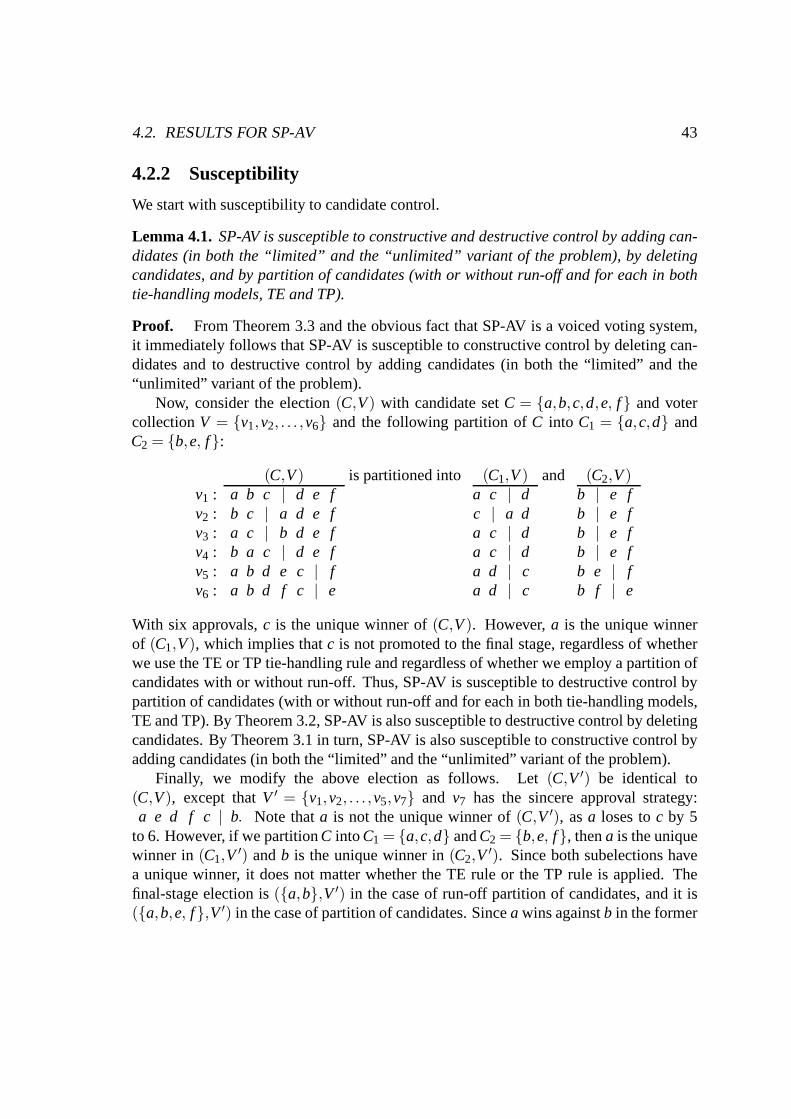
4.2. RESULTS FOR SP-AV 43
4.2.2 Susceptibility
We start with susceptibility to candidate control.
Lemma 4.1. SP-AV is susceptible to constructive and destructive control by adding can-didates (in both the “limited” and the “unlimited” variant of the problem), by deletingcandidates, and by partition of candidates (with or withoutrun-off and for each in bothtie-handling models, TE and TP).
Proof. From Theorem 3.3 and the obvious fact that SP-AV is a voiced voting system,it immediately follows that SP-AV is susceptible to constructive control by deleting can-didates and to destructive control by adding candidates (inboth the “limited” and the“unlimited” variant of the problem).
Now, consider the election(C,V) with candidate setC = {a,b,c,d,e, f} and votercollectionV = {v1,v2, . . . ,v6} and the following partition ofC into C1 = {a,c,d} andC2 = {b,e, f}:
(C,V) is partitioned into (C1,V) and (C2,V)v1 : a b c | d e f a c | d b | e fv2 : b c | a d e f c | a d b | e fv3 : a c | b d e f a c | d b | e fv4 : b a c | d e f a c | d b | e fv5 : a b d e c | f a d | c b e | fv6 : a b d f c | e a d | c b f | e
With six approvals,c is the unique winner of(C,V). However,a is the unique winnerof (C1,V), which implies thatc is not promoted to the final stage, regardless of whetherwe use the TE or TP tie-handling rule and regardless of whether we employ a partition ofcandidates with or without run-off. Thus, SP-AV is susceptible to destructive control bypartition of candidates (with or without run-off and for each in both tie-handling models,TE and TP). By Theorem 3.2, SP-AV is also susceptible to destructive control by deletingcandidates. By Theorem 3.1 in turn, SP-AV is also susceptible to constructive control byadding candidates (in both the “limited” and the “unlimited” variant of the problem).
Finally, we modify the above election as follows. Let(C,V′) be identical to(C,V), except thatV ′ = {v1,v2, . . . ,v5,v7} and v7 has the sincere approval strategy:a e d f c | b. Note thata is not the unique winner of(C,V ′), asa loses toc by 5
to 6. However, if we partitionC intoC1 = {a,c,d} andC2 = {b,e, f}, thena is the uniquewinner in (C1,V ′) andb is the unique winner in(C2,V ′). Since both subelections havea unique winner, it does not matter whether the TE rule or the TP rule is applied. Thefinal-stage election is({a,b},V′) in the case of run-off partition of candidates, and it is({a,b,e, f},V′) in the case of partition of candidates. Sincea wins againstb in the former
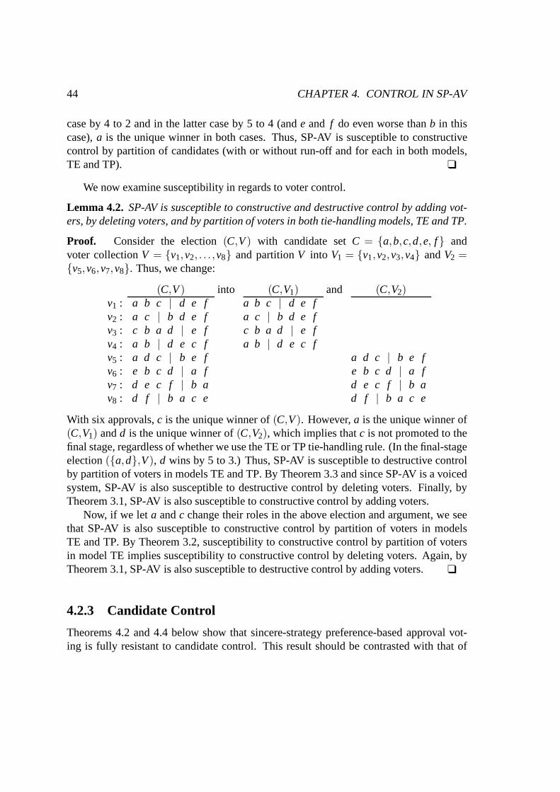
44 CHAPTER 4. CONTROL IN SP-AV
case by 4 to 2 and in the latter case by 5 to 4 (ande and f do even worse thanb in thiscase),a is the unique winner in both cases. Thus, SP-AV is susceptible to constructivecontrol by partition of candidates (with or without run-offand for each in both models,TE and TP). ❑
We now examine susceptibility in regards to voter control.
Lemma 4.2. SP-AV is susceptible to constructive and destructive control by adding vot-ers, by deleting voters, and by partition of voters in both tie-handling models, TE and TP.
Proof. Consider the election(C,V) with candidate setC = {a,b,c,d,e, f} andvoter collectionV = {v1,v2, . . . ,v8} and partitionV into V1 = {v1,v2,v3,v4} andV2 ={v5,v6,v7,v8}. Thus, we change:
(C,V) into (C,V1) and (C,V2)v1 : a b c | d e f a b c | d e fv2 : a c | b d e f a c | b d e fv3 : c b a d | e f c b a d | e fv4 : a b | d e c f a b | d e c fv5 : a d c | b e f a d c | b e fv6 : e b c d | a f e b c d | a fv7 : d e c f | b a d e c f | b av8 : d f | b a c e d f | b a c e
With six approvals,c is the unique winner of(C,V). However,a is the unique winner of(C,V1) andd is the unique winner of(C,V2), which implies thatc is not promoted to thefinal stage, regardless of whether we use the TE or TP tie-handling rule. (In the final-stageelection({a,d},V), d wins by 5 to 3.) Thus, SP-AV is susceptible to destructive controlby partition of voters in models TE and TP. By Theorem 3.3 and since SP-AV is a voicedsystem, SP-AV is also susceptible to destructive control bydeleting voters. Finally, byTheorem 3.1, SP-AV is also susceptible to constructive control by adding voters.
Now, if we let a andc change their roles in the above election and argument, we seethat SP-AV is also susceptible to constructive control by partition of voters in modelsTE and TP. By Theorem 3.2, susceptibility to constructive control by partition of votersin model TE implies susceptibility to constructive controlby deleting voters. Again, byTheorem 3.1, SP-AV is also susceptible to destructive control by adding voters. ❑
4.2.3 Candidate Control
Theorems 4.2 and 4.4 below show that sincere-strategy preference-based approval vot-ing is fully resistant to candidate control. This result should be contrasted with that of

4.2. RESULTS FOR SP-AV 45
Hemaspaandra, Hemaspaandra, and Rothe [HHR07a], who proved immunity and vul-nerability for all cases of candidate control within approval voting (see Table 4.1). Infact, SP-AV has the same resistances to candidate control asplurality, and we will showthat the construction presented in [HHR07a] to prove plurality resistant also works forsincere-strategy preference-based approval voting in allcases of candidate control exceptone—namely, except for constructive control by deleting candidates. Theorem 4.4 estab-lishes resistance for this one missing case.
All resistance results in this section follow via a reduction from the NP-complete prob-lem Hitting Set introduced in Section 2.2. Note that some of our proofs for SP-AV arebased on constructions and arguments presented in [HHR07a]to prove the correspond-ing results for approval voting or plurality, whereas the remainder of our results requirenew insights to make the proof work for SP-AV. For completeness, we will present eachconstruction here (even if the modification of a previous construction is rather straightfor-ward), noting the differences to the related previous constructions.
Theorem 4.2. SP-AV is resistant to all types of constructive and destructive candidatecontrol defined in Section 3.3 except for constructive control by deleting candidates.
Resistance of SP-AV to constructive control by deleting candidates, which is the miss-ing case in Theorem 4.2, will be shown as Theorem 4.4 below.
The proof of Theorem 4.2 is based on a construction for plurality in [HHR07a], exceptthat only the arguments fordestructivecandidate control are given there (simply becauseplurality was shown resistant to all cases of constructive candidate control already byBartholdi, Tovey, and Trick [BTT92] via different constructions). We now provide theproof of Theorem 4.2 and the construction from [HHR07a] (slightly modified so as to beformally conform with the SP-AV voter representation) in order to (i) show that the sameconstruction can be used to establish all but one resistances of SP-AV toconstructivecandidate control, and (ii) explain why constructive control by deleting candidates (whichis missing in Theorem 4.2) doesnot follow from this construction.
Proof of Theorem 4.2. Susceptibility holds by Lemma 4.1 in each case. The resistanceproofs are based on a reduction from Hitting Set and employ Construction 4.3 below,slightly modified so as to be formally conform with the SP-AV voter representation.
Construction 4.3 ([HHR07a]). Let (B,S ,k) be a given instance of Hitting Set, whereB= {b1,b2, . . . ,bm} is a set,S = {S1,S2, . . . ,Sn} is a collection of subsets Si ⊆B, and k≤m is a positive integer. Define the election(C,V), where C= B∪{c,w} is the candidateset and where V consists of the following voters:
1. There are2(m−k)+2n(k+1)+4 voters of the form:
c | w B.

46 CHAPTER 4. CONTROL IN SP-AV
2. There are2n(k+1)+5 voters of the form:
w | c B.
3. For each i,1≤ i ≤ n, there are2(k+1) voters of the form:
Si | c w (B−Si).
4. For each j,1≤ j ≤m, there are two voters of the form:
b j | w c (B−{b j}).
Sincescore({c,w},V)(c)−score({c,w},V)(w) = 2k(n−1)+2n−1 is positive (because ofn≥ 1),c is the unique winner of election({c,w},V). The key observation is the followingproposition, which can be proven as in [HHR07a].
Proposition 4.2([HHR07a]). 1. If S has a hitting set B′ of size k, then w is the uniqueSP-AV winner of election(B′∪{c,w},V).
2. Let D⊆ B∪{w}. If c is not the unique SP-AV winner of election(D∪{c},V), thenthere exists a set B′ ⊆ B such that
(a) D = B′∪{w},
(b) w is the unique SP-AV winner of election(B′∪{c,w},V), and
(c) B′ is a hitting set ofS of size less than or equal to k.
Proof.
1. Suppose thatB′ is a hitting set ofS of sizek. Then we have the following scoresin election(B′∪{c,w},V):
score(c) = 2(m−k)+2n(k+1)+4,score(w) = 2(m−k)+2n(k+1)+5,score(b j) ≤ 2n(k+1)+2 for eachj, 1≤ j ≤m.
Thus,w is the unique SP-AV winner of election(B′∪{c,w},V).
2. Let D ⊆ B∪ {w}. Supposec is not the unique SP-AV winner of election(D∪{c},V).

4.2. RESULTS FOR SP-AV 47
(a) Since for eachb∈ D∩B, score(D∪{c},V)(b) < score(D∪{c},V)(c), andc is notthe unique SP-AV winner of election(D∪{c},V), c can only lose the electionagainstw. Thus,D = B′∪{w}, whereB′ ⊆ B.
(b) This part follows immediatly from part(a).
(c) Let ` be the number of sets inS not hit byB′, then:
score(B′∪{c,w},V)(w) = 2n(k+1)+5+2(m−‖B′‖),score(B′∪{c,w},V)(c) = 2(m−k)+2n(k+1)+4+2(k+1)`.
From part (a) we know, thatscore(B′∪{c,w},V)(w)≥ score(B′∪{c,w},V)(c), i.e.,
2n(k+1)+5+2(m−‖B′‖)≥ 2(m−k)+2n(k+1)+4+2(k+1)`.
Since all variables are integers, the above inequality implies
0≥ ‖B′‖−k+(k+1)`
thus,` = 0, and soB′ is a hitting set ofS of size less than or equal tok.
❑
Corollary 4.1. SP-AV is resistant to constructive and destructive controlby adding can-didates (both in the limited and the unlimited version of theproblem).
Proof. This corollary follows immediately from Proposition 4.2, via mapping the Hit-ting Set instance(B,S ,k) to the set{c,w} of qualified candidates and the setB of spoilercandidates, to the voter collectionV, and by havingc be the designated candidate inthe destructive case and by havingw be the designated candidate in the constructivecase. ❑
Corollary 4.2. SP-AV is resistant to destructive control by deleting candidates.
Proof. Let the election(C,V) be given as in Construction 4.3 with distinguished candi-datec. We claim thatS has a hitting set of size at mostk, if and only ifc can be preventedfrom being a unique SP-AV winner by deleting at mostm−k candidates.
From left to right: Suppose,S has a hitting setB′ ⊆ B of size k. According toProposition 4.2,c is not the unique SP-AV winner of the election(B′∪{c,w},V). Thus,by deleting the setB−B′ of candidates, where‖B−B′‖ = m− k, c is prevented to be aunique SP-AV winner of the election.
From right to left: Suppose, thatccan be prevented from being a unique SP-AV winnerby deleting at mostm−k candidates. LetD ⊆ B∪{w} be the set of deleted candidates,such thatc /∈D. It immediately follows from Proposition 4.2, thatC−D−{c}= B′∪{w},whereB′ is a hitting set ofS of size at mostk. ❑

48 CHAPTER 4. CONTROL IN SP-AV
Corollary 4.3. SP-AV is resistant to constructive and destructive controlby partition ofcandidates and run-off partition of candidates (for each inboth models TE and TP).
Proof. We only prove the constructive case. Let the election(C,V) be given as inConstruction 4.3 with distinguished candidatew. We claim thatS has a hitting set ofsize at mostk, if and only if w can be made the unique SP-AV winner by partition orrun-off partition of candidates (for each in both models TE and TP).
From left to right: Suppose,S has a hitting setB′ ⊆ B of sizek. Partition the set ofcandidates into the two subsetsC1 = B′∪{c,w} andC2 = C−C1. According to Propo-sition 4.2,w is the unique SP-AV winner of the election(B′∪{c,w},V). Then, the scoreof w is at least 2(m−k)+4n(k+1)+9 in the final stage, and the score of any participantfrom the other subelection is at most 2n(k+ 1)+ 2, thusw is the unique winner of theelection.
From right to left: Suppose, there exists a partition such that w is the unique SP-AVwinner of the election. In this case,c is not the unique SP-AV winner of the election.Then, there has to be a subsetD ⊆ B∪{w} of candidates such thatc is not the uniqueSP-AV winner of the election(D∪{c},V). Due to Proposition 4.2, there exists a sizekhitting set ofS .
For the destructive case simply change the roles ofc andw. ❑
Corollaries 4.1, 4.2, and 4.3 complete the proof for Theorem4.2. ❑ Theorem 4.2
Turning now to the missing case mentioned in Theorem 4.2 above: Why does Con-struction 4.3 not work for constructive control by deletingcandidates? Informally put, thereason is thatc is the only serious rival ofw in the election(C,V) of Construction 4.3,so by simply deletingc the chair could makew the unique SP-AV winner, regardless ofwhetherS has a hitting set of sizek. However, via a different construction, we can proveresistance also in this case.
Theorem 4.4.SP-AV is resistant to constructive control by deleting candidates.
Proof. Susceptibility holds by Lemma 4.1. To prove resistance, we provide a re-duction from Hitting Set. Let(B,S ,k) be a given instance of Hitting Set, whereB = {b1,b2, . . . ,bm} is a set,S = {S1,S2, . . . ,Sn} is a collection of subsetsSi ⊆ B, andk < m is a positive integer.4
Define the election(C,V), whereC = B∪{w} is the candidate set andV is the col-lection of voters. We assume that the candidates inB are in an arbitrary but fixed order,and for each voter below, this order is also used in each subset of B. For example, if
4Note that if k = m then B is always a hitting set of size at mostk (provided thatS contains onlynonempty sets—a requirement that doesn’t affect the NP-completeness of the problem), and we thus mayrequire thatk < m.

4.2. RESULTS FOR SP-AV 49
B = {b1,b2,b3,b4} and some subsetSi = {b1,b3} of B occurs in some voter then thisvoter prefersb1 to b3, and so does any other voter whose preference list containsSi .
V consists of the following 4n(k+1)+4m−2k+3 voters:
1. For eachi, 1≤ i ≤ n, there are 2(k+1) voters of the form:
Si | (B−Si) w.
2. For eachi, 1≤ i ≤ n, there are 2(k+1) voters of the form:
(B−Si) w | Si .
3. For eachj, 1≤ j ≤m, there are two voters of the form:
b j | w (B−{b j}).
4. There are 2(m−k) voters of the form:
B | w.
5. There are three voters of the form:
w | B.
Since for eachb j ∈ B, the difference
score(C,V)(w)−score(C,V)(b j) = 2n(k+1)+3−(2n(k+1)+2+2(m−k)) = 1−2(m−k)
is negative (due tok < m), w loses to each member ofB and so does not win election(C,V).
We claim thatS has a hitting setB′ of sizek if and only if w can be made the uniqueSP-AV winner by deleting at mostm−k candidates.
From left to right: SupposeS has a hitting setB′ of sizek. Then, for eachb j ∈ B′,
score(B′∪{w},V)(w)−score(B′∪{w},V)(b j) =
2n(k+1)+2(m−k)+3− (2n(k+1)+2+2(m−k)) = 1,
since the approval line is moved for 2(m−k) voters in the third group, thus transferringtheir approvals from members ofB−B′ to w. Sow is the unique SP-AV winner of election(B′∪{w},V). SinceB′∪{w}= C− (B−B′), it follows from ‖B‖= m and‖B′‖= k thatdeletingm−k candidates fromC makesw the unique SP-AV winner.

50 CHAPTER 4. CONTROL IN SP-AV
From right to left: LetD ⊆ B be any set such that‖D‖ ≤m− k andw is the uniqueSP-AV winner of election(C−D,V). Let B′ = (C−D)−{w}. Note thatB′ ⊆ B and thatwe have the following scores in(B′∪{w},V):
score(B′∪{w},V)(w) = 2(n− `)(k+1)+2(m−‖B′‖)+3,
score(B′∪{w},V)(b j) ≤ 2n(k+1)+2(k+1)`+2+2(m−k) for eachb j ∈ B′,
where` is the number of setsSi ∈S that are not hit byB′, i.e.,B′∩Si = /0. Recall thatfor eachi, 1≤ i ≤ n, all of the 2(k+1) voters of the form Si | (B−Si) w in the firstvoter group have ranked the candidates in the same order. Thus, for eachi, 1≤ i ≤ n,wheneverB′∩Si = /0 one and the same candidate inB′ benefits from moving the approvalline, namely the candidate occurring first in our fixed ordering ofB′. Call this candidateband note that
score(B′∪{w},V)(b) = 2n(k+1)+2(k+1)`+2+2(m−k).
Sincew is the unique SP-AV winner of(B′ ∪ {w},V), w has more approvals than anycandidate inB′ and in particular more thanb. Thus, we have
score(B′∪{w},V)(w)−score(B′∪{w},V)(b)
= 2(n− `)(k+1)+2(m−‖B′‖)+3−2n(k+1)−2`(k+1)−2−2(m−k)
= 1+2(k−‖B′‖)−4`(k+1) > 0.
Solving this inequality for , we obtain
0≤ ` <1+2(k−‖B′‖)
4(k+1)<
4+4k4(k+1)
= 1.
Thus` = 0. It follows that 1+ 2(k−‖B′‖) > 0, which implies‖B′‖ ≤ k. Thus,B′ is ahitting set of size at mostk. ❑
4.2.4 Voter Control
Turning now to control by adding and by deleting voters, it isknown from [HHR07a] thatapproval voting is resistant to constructive control and isvulnerable to destructive control(see Table 4.1).5 These proofs can be modified so as to also apply to sincere-strategypreference-based approval voting.
5Procaccia, Rosenschein, and Zohar [PRZ07] proved in their interesting “multi-winner” model (whichgeneralizes Bartholdi, Tovey, and Trick’s model [BTT92] byadding a utility function and some other pa-rameters) that approval voting is resistant to constructive control by adding voters. According to Foot-note 13 of [HHR07a], this resistance result immediately follows from the corresponding resistance result in[HHR05, HHR07a], essentially due to the fact that lower bounds in more flexible models are inherited frommore restrictive models.

4.2. RESULTS FOR SP-AV 51
Theorem 4.5.SP-AV is resistant to constructive control by adding votersand by deletingvoters and is vulnerable to destructive control by adding voters and by deleting voters.
Proof. Susceptibility holds by Lemma 4.2 in all cases. To prove resistance to con-structive control by adding voters (respectively, by deleting voters), the construction of[HHR07a, Thm. 4.43] (respectively, of [HHR07a, Thm. 4.44])works, modified only byspecifying voter preferences consistently with the voters’ approval strategies (and, in thedeleting-voters case, by adding a dummy candidate who is disapproved and ranked lastby every voter in the construction to ensure an admissible AVstrategy profile). Theseconstructions provide polynomial-time reductions from the NP-complete problem ExactCover by Three-Sets defined in Section 2.2.
We now give the proof for these two resistance results. In both cases, we start from anX3C instance(B,S ).
In the case of constructive control by adding voters, for a given X3C instance(B,S ),whereB = {b1,b2, . . . ,b3m}, m> 1, is a set andS = {S1,S2, . . . ,Sn} is a collection ofsubsetsSi ⊆ B with ‖Si‖= 3 for eachi, we define the election(C,V), with candidate setC = B∪{w} and withV consisting ofm−2 registered voters each of the form
B | w.
Further, we defineW to consist of the followingn unregistered voters: For eachi, 1≤ i ≤n, there is one voter of the form
w Si | (B−Si).
We claim thatS has an exact cover forB if and only if w can be made the uniqueSP-AV winner by adding at mostm voters.
From left to right: SupposeS contains an exact cover forB. Add them voters ofWcorresponding to this exact cover toV. LetW′ ⊆W be the set of unregistered voters thusadded. Thenscore(C,V∪W′)(w) = m andscore(C,V∪W′)(bi) = m−1 for all 1≤ i ≤ 3m, sow is the unique winner.
From right to left: LetW′ be any subset ofW such that‖W′‖ ≤mandw is the uniquewinner of the election(C,V ∪W′). It follows that‖W′‖ = m, and eachbi ∈ B can gainonly one point. Thus, them voters inW′ correspond to an exact cover forB.
In the case of constructive control by deleting voters, define the value j = ‖{Si ∈S |b j ∈ Si}‖ for eachj, 1≤ j ≤ 3m. Define the election(C,V), whereC = B∪{w,d} isthe set of candidates,w is the distinguished candidate, andV is the following collectionof 2n voters:
1. For eachi, 1≤ i ≤ n, there is one voter of the form:
Si | (B−Si) w d.

52 CHAPTER 4. CONTROL IN SP-AV
2. For eachi, 1≤ i ≤ n, there is one voter of the form:
w Bi | (B−Bi) d,
whereBi = {b j ∈ B| i ≤ n− ` j}.
Note thatscore(C,V)(w) = n andscore(C,V)(b j) = n for all b j ∈ B.We claim thatS has an exact cover forB if and only if w can be made the unique
SP-AV winner by deleting at mostm voters.From left to right: SupposeS contains an exact cover forB. Delete them voters
corresponding to this exact cover. LetV ′ ⊆ V be the set of voters thus deleted. Thenscore(C,V−V ′)(w) = n, score(C,V−V ′)(d) < n, andscore(C,V−V ′)(b j) = n−1 for all b j ∈ B.Thusw is the unique winner.
From right to left: LetV ′ be any subset ofV such that‖V ′‖ ≤m andw is the uniquewinner of the election(C,V−V ′). We can assume that the voters corresponding toV ′
have disapproved of the distinguished candidatew. Since each candidateb j ∈ B mustlose at least one point and by our assumption that only votersfrom the first group havebeen deleted, it follows that the deleted voters correspondto a cover. Since the number ofdeleted voters is at mostm, they correspond to an exact cover forB.
The polynomial-time algorithms showing that approval voting is vulnerable to de-structive control by adding voters and by deleting voters [HHR07a, Thm. 4.24] can bestraightforwardly adapted to also work for sincere-strategy preference-based approval vot-ing, since no approval lines are moved in these control scenarios. For completeness, weprovide these proofs.
In the case of destructive control by adding voters, the input to the algorithm is anelection(C,V), a collectionW of additional voters (where each voterv in V ∪W has asincere AV strategySv with /0 6= Sv 6= C), a distinguished candidatec∈C, and a nonneg-ative integer . The output will be either a subsetW′ ⊆W of voters such that‖W′‖ ≤ `,and adding the voters ofW′ to V ensures thatc is not a unique winner, or it will be“control impossible” if no such subset exists. IfC = {c} then output “control impossi-ble” and halt, since one candidate is always the unique winner independent of the num-ber of voters. If‖C‖ > 1 andc is already not the unique SP-AV winner of the elec-tion (C,V) then outputW′ = /0 and halt. Otherwise, for each candidated 6= c definesurplus(c,d) = score(c)− score(d). Among all candidatesi 6= c such that there existsurplus(C,V)(c, i) voters inW who approve ofi and who disapprove ofc, let j be one suchcandidate for whichsurplus(C,V)(c, j) is minimum. Output thesurplus(C,V)(c, j) votersfromW who approve ofj and disapprove ofc. If there is no such candidatej, then output“control impossible” and halt.
In the case of destructive control by deleting voters, the input to the algorithm is anelection(C,V) (where each voterv ∈ V has a sincere AV strategySv with /0 6= Sv 6= C),

4.2. RESULTS FOR SP-AV 53
a distinguished candidatec∈C, and a nonnegative integer`. The output will be either asubsetV ′ ⊆V of voters such that‖V ′‖ ≤ ` and deleting the voters ofV ′ from V ensuresthatc is not a unique winner, or it will be “control impossible” if no such subset exists. IfC = {c} then again output “control impossible” and halt. If‖C‖> 1 andc already is nota unique SP-AV winner of the election(C,V), then outputV ′ = /0 and halt. Otherwise, letj 6= c be the candidate for whomsurplus(C,V)(c, j) is minimum. If surplus(C,V)(c, j) > `then output “control impossible” and halt. Otherwise, output thesurplus(C,V)(c, j) votersfrom V who approve ofc and disapprove ofj. ❑
We now prove that, just like plurality, sincere-strategy preference-based approval vot-ing is resistant to constructive and destructive control bypartition of voters in model TP.In fact, the proof presented in [HHR07a] for plurality in these two cases also works forSP-AV with minor modifications. In contrast, approval voting is vulnerable to the destruc-tive variant of this control type [HHR07a].
Theorem 4.6. SP-AV is resistant to constructive and destructive controlby partition ofvoters in model TP.
Proof. The proof is again based on Construction 4.3, but the reduction is now fromRestricted Hitting Set (see Section 2.2). Now, the key observation is the following propo-sition, which can be proven as in [HHR07a].
Proposition 4.3 ([HHR07a]). Let (B,S ,k) be a given Restricted Hitting Set instance,where B= {b1,b2, . . . ,bm} is a set,S = {S1,S2, . . . ,Sn} is a collection of subsets Si ⊆ B,and k≤ m is a positive integer such that n(k+ 1)+ 1≤ m− k. If (C,V) is the electionresulting from(B,S ,k) via Construction 4.3, then the following three statements areequivalent:
1. S has a hitting set of size less than or equal to k.
2. V can be partitioned such that w is the unique SP-AV winner in model TP.
3. V can be partitioned such that c is not the unique SP-AV winner in model TP.
Proof. It is trivial that if V can be partitioned such thatw is the unique SP-AV winner inmodel TP, thenc is not the unique SP-AV winner. Thus, statement two implies statementthree.
Let (B,S ,k) be a given Restricted Hitting Set instance as defined above inProposi-tion 4.3. Suppose, thatS has a hitting setB′ of size less than or equal tok. PartitionV into V1 andV2 such thatV1 consists of one voter of the formc | w B, and for eachb j ∈ B′ one voter of the form b j | w c (B−{b j}), andV2 = V −V1. The winnersof subelection(C,V1) are all candidates corresponding toB′ andw, since they all have
54 CHAPTER 4. CONTROL IN SP-AV
a score of 1, all the other candidates have no points at all. Inthe second subelection(C,V2), c is the unique winner, sincescore(C,V2)(b j)≤ 2n(k+1)+2 for each 1≤ j ≤ n,score(C,V2)(w) = 2n(k+1)+5, andscore(C,V2)(c) = 2(m−k)+2n(k+1)+3. Note, thatscore(C,V2)(c)−score(C,V2)(w) = 2(m−k−1) > 0 due to the restriction in the RestrictedHitting Set instance. By Proposition 4.2,w is the unique SP-AV winner of the final stage.This proves that the first statement implies the second and third statements.
Showing that statement three implies statement one will complete the proof. Supposethere is a partition ofV intoV1 andV2 such thatc is not the unique SP-AV winner in the TPmodel. We claim thatc is an SP-AV winner of one of the subelections(C,V1) or (C,V2).For a contradiction, suppose thatc is not a winner in both subelections. Then, there haveto be two candidatesx,y∈ B∪{w} such that candidatex is the winner of(C,V1) andy isthe winner of(C,V2). Then, the following holds:
(4.2.1)score(C,V1)(x)+score(C,V2)(y) ≥ score(C,V1)(c)+score(C,V2)(c)+2
≥ score(C,V)(c)+2.
Sincec has the highest score of all candidates in(C,V), we havex 6= y. Then,
score(C,V1)(x)+score(C,V2)(y) ≤ score(C,V)(w)+score(C,V)(b j)≤ 2n(k+1)+5+2n(k+1)+2≤ 2n(k+1)+5+2(m−k)≤ score(C,V)(c)+1,
which contradicts to Equation 4.2.1. Thus,c is a winner of one of the subelections(C,V1)or (C,V2) and will participate in the final round of the election.
Sincec is not a unique SP-AV winner of the final stage of the election(D∪{c},V),whereD ⊆ B∪ {w}, by Proposition 4.2,S has a hitting set of size less than or equalto k. ❑
Theorem 4.6 now follows immediately from Proposition 4.3. ❑ Theorem 4.6
Finally, we turn to control by partition of voters in model TE. For this control type,Hemaspaandra et al. [HHR07a] proved approval voting resistant in the constructive caseand vulnerable in the destructive case. We have the same results for sincere-strategypreference-based approval voting. Our resistance proof inthe constructive case (see theproof of Theorem 4.7) is similar to the corresponding proof of resistance in [HHR07a].However, while our polynomial-time algorithm showing vulnerability for SP-AV in thedestructive case (see the proof of Theorem 4.8) is based on the corresponding polynomial-time algorithm for approval voting in [HHR07a], it extends their algorithm in a nontrivialway.

4.2. RESULTS FOR SP-AV 55
Theorem 4.7. SP-AV is resistant to constructive control by partition of voters inmodel TE.
Proof. Susceptibility holds by Lemma 4.2. The proof of resistance is based on theconstruction of [HHR07a, Thm. 4.46] with only minor changes. Let an X3C instance(B,S ) be given, whereB = {b1,b2, . . . ,b3m}, m> 1, is a set andS = {S1,S2, . . . ,Sn} isa collection of subsetsSi ⊆B with ‖Si‖= 3 for eachi. Without loss of generality, we mayassume thatn≥m. Define the value j = ‖{Si ∈S |b j ∈ Si}‖ for each j, 1≤ j ≤ 3m asin the proof of Theorem 4.5.
Define the election(C,V), whereC = B∪{w,x,y}∪Z is the candidate set with thedistinguished candidatew, Z = {z1,z2, . . . ,zn}, and whereV is defined to consist of thefollowing 4n+mvoters:
1. For eachi, 1≤ i ≤ n, there is one voter of the form:
y Si | w ((B−Si)∪{x}∪Z).
2. For eachi, 1≤ i ≤ n, there is one voter of the form:
y zi | w (B∪{x}∪ (Z−{zi})).
3. For eachi, 1≤ i ≤ n, there is one voter of the form:
w (Z−{zi}) Bi | x y zi (B−Bi),
whereBi = {b j ∈ B| i ≤ n− ` j}.
4. There aren+m voters of the form:
x | y (B∪{w}∪Z).
Since the above construction is only slightly modified from the proof of [HHR07a,Thm. 4.46], so as to be formally conform with the SP-AV voter representation, the sameargument as in that proof shows thatS has an exact cover forB if and only if w canbe made the unique SP-AV winner by partition of voters in model TE. Note that, in thepresent control scenario, approval voting and SP-AV can differ only in the run-off, but theconstruction ensures that they don’t differ there.
From left to right, ifS has an exact cover forB then partition the set of voters asfollows: V1 consists of them voters of the formy Si | w ((B−Si)∪{x}∪Z) that cor-respond to the sets in the exact cover, of then+m voters who approve of onlyx, and ofthe n voters who approve ofy andzi, 1≤ i ≤ n. Let V2 = V −V1. It follows thatw is

56 CHAPTER 4. CONTROL IN SP-AV
the unique SP-AV winner of both subelection(C,V2) and the run-off, simply because nocandidate proceeds to the run-off from the other subelection, (C,V1), in whichx andy tiefor winner with a score ofn+m each.
From right to left, supposew can be made the unique SP-AV winner by par-tition of voters in model TE. Let(V1,V2) be a partition ofV such thatw is theunique SP-AV winner of the run-off. According to model TE,w must also be theunique SP-AV winner of one subelection, say of(C,V1). Note that each voter ofthe form y zi | w (B∪{x}∪ (Z−{zi})) has to be inV2 (otherwise, we would havescore(C,V1)(w) = score(C,V1)(zi) for at least onei, and sow would not be the uniqueSP-AV winner of(C,V1) anymore). However, if there were more thanm voters of theform y Si | w ((B−Si)∪{x}∪Z) in V2 then score(C,V2)(y) > n+ m, and soy wouldbe the unique SP-AV winner of the other subelection,(C,V2). But then, also in theSP-AV model,y would win the run-off againstw becausescore({w,y},V)(y) = 3n+ m>n = score({w,y},V)(w), which contradicts the assumption thatw has been made the uniqueSP-AV winner by the partition(V1,V2). Hence, there are at mostm voters of the formy Si | w ((B−Si)∪{x}∪Z) in V2, and thesem voters correspond to an exact coverof B. ❑
Theorem 4.8. SP-AV is vulnerable to destructive control by partition of voters inmodel TE.
Proof. Susceptibility holds by Lemma 4.2. To prove vulnerability,we describe apolynomial-time algorithm showing that (and how) the chaircan exert destructive con-trol by partition of voters in model TE for sincere-strategypreference-based approval vot-ing. Our algorithm extends the polynomial-time algorithm designed by Hemaspaandraet al. [HHR07a] to prove approval voting vulnerable to this type of control. Specifically,our algorithm adds Loop 2 below to their algorithm, and we will explain below why it isnecessary to add this second loop.
We adopt the following notation from [HHR07a]. Let(C,V) be an election, and foreach voterv ∈ V, let Sv ⊆C denotev’s AV strategy. In each iteration of Loop 1 in thealgorithm below, we will consider three candidates,a, b, andc. Define the following fivenumbers:
Wc = ‖{v∈V |a 6∈ Sv, b 6∈ Sv, c∈ Sv}‖, Lc = ‖{v∈V |a∈ Sv, b∈ Sv, c 6∈ Sv}‖,
Da = ‖{v∈V |a∈ Sv, b 6∈ Sv, c 6∈ Sv}‖, Db = ‖{v∈V |a 6∈ Sv, b∈ Sv, c 6∈ Sv}‖, and
Dac = ‖{v∈V |a∈ Sv, b 6∈ Sv, c∈ Sv}‖.
In addition, we introduce the following notation. Given an election (C,V) and twodistinct candidatesx,y∈C, let diff (x,y) denote the number of voters inV who preferx to

4.2. RESULTS FOR SP-AV 57
y minus the number of voters inV who prefery to x. DefineBx to be the set of candidatesy 6= x in C such thatdiff (y,x)≥ 0.
The input to our algorithm is an election(C,V), where each voterv∈V has a sincereAV strategySv with /0 6= Sv 6=C (otherwise, the input is considered malformed and outrightrejected), and a distinguished candidatec ∈ C. On this input, our algorithm works asfollows.
1. Checking the trivial cases: can be done as in the case of approval voting, seethe proof of [HHR07a, Thm. 4.21]. In particular, ifC = {c} then output “controlimpossible” and halt, sincec cannot help but win. IfC contains more candidatesthan onlyc but c already is not the unique SP-AV winner in(C,V) then output the(successful) partition(V, /0) and halt. Otherwise, if‖C‖ = 2 then output “controlimpossible” and halt, asc is the unique SP-AV winner of(C,V) in the current case,and so, however the voters are partitioned,c must win—against the one rivallingcandidate—at least one subelection and also the run-off.
2. Loop 1: For eacha,b∈C such that‖{a,b,c}‖= 3, check whetherV can be parti-tioned intoV1 andV2 such thatscore(C,V1)(a)≥ score(C,V1)(c) andscore(C,V2)(b)≥score(C,V2)(c). As shown in the proof of [HHR07a, Thm. 4.21], this is equivalent tochecking
Wc−Lc≤Da +Db.(4.2.2)
If (4.2.2) fails, thisa andb cannot preventc from being the unique winner of atleast one subelection and thus also of the run-off, so we moveon to test the nextaandb in this loop. If (4.2.2) holds, however, output the partition (V1,V2) and halt,whereV1 consists of the voters contributing toDa, of the voters contributing toDac,and of min(Wc,Da) voters contributing toWc, and whereV2 = V−V1.
3. Loop 2: For eachd ∈ Bc, partitionV as follows. LetV1 consist of all voters inVwho approve ofd, and letV2 = V−V1. If d is the unique winner of(C,V1), thenoutput(V1,V2) as a successful partition and halt. Otherwise, go to the nextd ∈ Bc.
4. Termination: If in no iteration of either Loop 1 or Loop 2 a successful partition ofV was found, then output “control impossible” and halt.
Let us give a short explanation of why Loop 2 is needed for SP-AV by stressing thedifference with approval voting. As shown in the proof of [HHR07a, Thm. 4.21], ifnone of the trivial cases applied, then condition (4.2.2) holds for somea,b ∈ C with‖{a,b,c}‖ = 3 if and only if destructive control by partition of voters inmodel TE ispossible for approval voting. Thus, for approval voting, ifLoop 1 was not successful

58 CHAPTER 4. CONTROL IN SP-AV
for any sucha and b, we may immediately jump to the termination stage, where thealgorithm outputs “control impossible” and halts. In contrast, if none of the trivial casesapply, then the existence of candidatesa andb with ‖{a,b,c}‖ = 3 who satisfy (4.2.2)is not equivalent to destructive control by partition of voters inmodel TE being possiblefor SP-AV: it is a sufficient, yet not a necessary condition. The reason is that even ifthere are no candidatesa andb who can preventc from winning one subelection (in somepartition of voters) and from proceeding to the run-off, it might still be possible thatcloses or ties the run-off due to our rule of moving the approval line in order to re-enforceour conventions for SP-AV in this control scenario.
Indeed, if Loop 1 was not successful,c will lose or tie the run-off exactly if thereexists a candidated 6= c such thatdiff (d,c)≥ 0 andd can win one subelection (for somepartition of voters). This is precisely what is being checked in Loop 2. Indeed, notethat the partition(V1,V2) chosen in Loop 2 ford ∈ Bc is the best possible partition ford in the following sense: Ifd is not the unique SP-AV winner of subelection(C,V1)then, for eachW ⊆ V, d is not the unique SP-AV winner of subelection(C,W). To seethis, simply note that ifd is not the unique SP-AV winner of(C,V1), then there is somecandidatex with score(C,V1)(x) = score(C,V1)(d) = ‖V1‖, which by our choice ofV1 impliesscore(C,W)(x)≥ score(C,W)(d) for each subsetW ⊆V. ❑
Comparing Theorem 4.6 and Theorem 4.8, one can see that destrutive control bypartition of voters in SP-AV yield different results depending on the tie-handling ruleused.
4.3 Bribery and Manipulation in SP-AV
Faliszewski et al. [FHH06a] introduced the problem of bribery for voting systems. In thisscenario, an external agent seeks to influence the outcome ofan election by bribing someof the voters so as to change their preferences over the candidates.
Faliszewski et al. [FHH06a, FHH06c] proved that approval voting is resistant to con-structive bribery (even in the unweighted, unpriced variant of the problem). Since thevoters’ approval lines are not moved in bribery (as the number of candidates remainsunchanged), the same result for SP-AV can be shown analogously.
Theorem 4.9.SP-AV is resistant to constructive bribery.
Faliszewski et al. showed the NP-hardness of constructive approval-bribery via reduc-tion from the NP-complete problem X3C (see Section 2.2).
In contrast, Theorem 4.10 below shows vulnerability to destructive bribery for ap-proval voting and SP-AV, even in the weighted, priced variant of the problem.
4.3. BRIBERY AND MANIPULATION IN SP-AV 59
Theorem 4.10.Both approval voting and SP-AV are vulnerable to destructive bribery,even in the weighted, priced version of the problem.
Proof. Again, since the voters’ approval lines are not moved in bribery, it is enoughto prove the theorem for approval voting; an analogous proofalso works for SP-AV. Wedescribe a polynomial-time greedy algorithm that determines how the briber can bribesome voters, without exceeding his or her budget, such that adistinguished candidate willnot be a unique approval winner if that is at all possible.
We introduce the following notation. Letwv denote the weight and letpv denotethe price of voterv. Let a andb be any two distinct candidates in an electionE withscoreE(a) > scoreE(b). Define thecost-effectiveness of voter v for the candidates a and bby
CEv(a,b) =
pv
2wvif a is approved andb is disapproved byv
pv
wvif either botha andb are approved or botha andb are disapproved
∞ otherwise.
The cost-effectiveness gives us the price per unit weight that b can gain ona when voterv is being bribed suitably. We saya voter vi is more cost-effective than a voter vj if vi ’scost-effectiveness is less thanv j ’s. The input of the algorithm is an election(C,V), withdistinguished candidatec∈C, and a budgetk. Recall that each voterv∈V has a nontrivialsincere AV strategySv with /0 6= Sv 6= C, a weightwv and a pricepv. The algorithm worksas follows:
(1) Trivial cases: If C = {c} then output “bribery impossible” and halt, since there isno other candidate who could win the election. Ifc is already not the unique winnerthen output the given AV strategy profile for(C,V) and halt.
(2) Loop: For each candidatea∈C, compute the cost-effectiveness CEv(c,a) for eachvoter v ∈ V. Keep bribing the most cost-effective voterv as long as the budgetkis not exceeded in the following way: If (c is approved anda is disapproved byv)or (bothc anda are approved byv) or (bothc anda are disapproved byv) thenbribe v to approve ofa and to disapprove ofc. If this makes sure thatc isn’t theunique winner anymore, then output the thus modified AV strategy profile and halt.Otherwise go to the nexta∈C.
(3) Termination: If we haven’t found a candidatea in any loop iteration, such that wecould successively bribe voters to reach our goal, then output “bribery impossible”and halt.

60 CHAPTER 4. CONTROL IN SP-AV
Let us give a short explanation of the loop. Since the distinguished candidatec hasa surplus ofscore(C,V)(c)−score(C,V)(a) points against candidatea, the briber wishes tobuy at least that many points as cheap as possible. This is exactly what the loop does:The briber seeks greedily to bribe the cheapest voters, one after the other, until either thebudget limitk is exceeded (in which case the algorithm halts without success) or until thebribery was performed successfully. ❑
Note that our algorithm presented not only solves the decision problem for destructivebribery but also determines how to successfully bribe if that is possible.
We are turning now our attention to manipulation.
Theorem 4.11.Constructive and destructive approval-manipulation, approval-weighted-manipulation, SP-AV-manipulation and SP-AV-weighted-manipulation are inP.
Proof. We only give the proof for constructive SP-AV-weighted-manipulation. Let(C,V ∪V ′) be an election, whereC is the set of candidates,V = {v1,v2, . . . ,vn} is thecollection of voters who already cast their votes,V ′ = {vn+1,vn+2, . . . ,vn+m} is the col-lection of manipulators, letc∈C be the distinguished candidate, and letwi be the weightassigned to votervi ∈V ∪V ′ with 1≤ i ≤ n+m.
If score(C,V)(c) > score(C,V)(x) for eachx∈C with x 6= c, then each manipulator putsc left of the approval line. This way, no candidate can get closer toc, thusc is the uniqueSP-AV winner of election(C,V ∪V ′). Otherwise, there is at least one candidatex ∈Cwith score(C,V)(c)≤ score(C,V)(x). Let x be a candidate with highest score in(C,V). If
score(C,V)(x)−score(C,V)(c)≥m
∑i=n+1
wi ,
then it is impossible for the manipulators to make candidatec the unique SP-AV winner,sincec can gain on at most∑m
i=n+1wi points. Otherwise, the manipulators’ votes have thefollowing form:
c | (C−{c}).
Clearly,c gains on∑mi=n+1wi points, all the other candidates get no points at all. Thus,
c is then the unique SP-AV winner.The destructive cases goes analogously with the differencethat if it is possible to make
c not a unique SP-AV winner, then the manipulators cast their votes in the following way:
(C−{c}) | c.
Clearly, the algorithm runs in polynomial time and it again not only solves the decisionproblem for constructive weighted manipulation but also determines how to successfullymanipulate if that is possible.

4.4. CONCLUSIONS AND OPEN QUESTIONS 61
Since SP-AV-manipulation is the single weight special caseof SP-AV-weighted-manipulation, it follows that SP-AV-manipulation is also in P. ❑
4.4 Conclusions and Open Questions
We have shown that Brams and Sanver’s SP-AV system [BS06] is resistant to 19 ofthe 22 previously studied types of control. On the one hand, like Copeland voting[FHHR08b], SP-AV is fully resistant to constructive control, yet unlike Copeland itadditionally is broadly resistant to destructive control.On the other hand, like plural-ity [BTT92, HHR07a], SP-AV is fully resistant to candidate control, yet unlike plurality itadditionally is broadly resistant to voter control. Thus, for these 22 types of control, SP-AV has more resistances, by three, and fewer vulnerabilities to control than is currentlyknown for any other natural voting system with a polynomial-time winner problem.
We have also shown that both approval voting and SP-AV are vulnerable to destructivebribery, even when weights and prices are assigned to the voters.
An interesting open direction is to investigate control in SP-AV or even in any othervoting system in a parameterized point of view. That is, for example, fix the numberof candidates allowed to delete, is the resulting problem fixed-parameter tractable or in-tractable?
The main open question is still if there is a natural voting system with an easy winner-determination procedure which is resistant against any control action. In the followingchapter we will investigate fallback voting with respect toour 22 control actions.

62 CHAPTER 4. CONTROL IN SP-AV

Chapter 5
Control in Fallback Voting
This chapter considers in detail the second voting system introduced by Brams and San-ver [BS06], that combines approval and preference-based voting, with respect to our 22control actions.
5.1 Definitions and Conventions
We start with the definition of fallback voting.
Definition 5.1 ([BS06]). Let (C,V) be an election, where the voters both indicate ap-provals/disapprovals of the candidates. For each voter v∈ V, an AV strategy ofv isdefined analogously to SP-AV as a subset Sv⊆C such that v approves of all candidates inSv and disapproves of all candidates in C−Sv. Each voter v∈V also provides a tie-freelinear ordering of all candidates in Sv. The list of AV strategies for all voters in V is againcalled anAV strategy profile for(C,V).
For each c∈C, let score(C,V)(c) = ‖{v ∈ V | c ∈ Sv}‖ denote the number of c’s ap-provals, and let scorei(C,V)(c) be thelevel i score ofc which is the number of c’s approvals
ranked on ith position or higher.Winner determination:
1. On the first level, only the highest ranked approved candidates are considered. Ifthere is a candidate c∈C who has strict majority on this level, then c is the uniquelevel 1 FV winner of the election.
2. If there is no level 1 winner, the two highest ranked approved candidates are con-sidered in each approval strategy. If there is exactly one candidate c∈C who hasstrict majority on this level, then c is the unique level 2 FV winner of the election.
63
64 CHAPTER 5. CONTROL IN FALLBACK VOTING
If there are at least two candidates with strict majority, then a level 2 FV winner isa candidate with the highest level 2 score.
3. If there is no level 1 or level 2 winner, the voters descend level by level to lowerlevels until there is at least one candidate who was approvedby the strict majorityof the voters. Denote this level by level i. If there is only one such candidate, heor she is the unique level i FV winner of the election. If thereare more than onecandidates with strict majority, then a candidate with the highest level i score is alevel i FV winner of the election.
4. Otherwise, every candidate with the highest score(C,V)(c) is a winner of elec-tion (C,V).
Note that a level 1 FV winner is always the unique FV winner of an election. In con-trast to sincere-strategy preference-based approval voting, in fallback voting, regardlessof the control action, no changes have to be made on the ballots. Analogously to SP-AV,we also require sincerity in fallback voting, but unlike SP-AV, fallback voting allows for avoter to have an empty approval strategy, i.e.,Sv = /0 or even a complete approval strategy,thus,Sv = C, i.e., admissibility is not required.
We will represent votes in fallback voting like in SP-AV withthe difference that allcandidates right from the approval line are represented as aset without ranking (e.g.,“a b | {c,d}” means thata andb are approved of anda is ranked first place,b is rankedsecond, whereasc andd are both disapproved of, and they are not ranked).
Fallback voting, like SP-AV, does not satisfy Unique-WARP.
Proposition 5.1. Fallback voting does not satisfy Unique-WARP.
Proof. Consider the election(C,V) with candidate setC = {a,b,c,d} and voter collec-tionV = {v1,v2, . . . ,v6}:
v1 = v2 = v3 : a c | {b, d}v4 = v5 : b d c | {a}
v6 : d a c | {b}
There is no level 1 FV winner, and the unique level 2 FV winner of the election(C,V)is candidatea with score2(C,V)(a) = 4. By removing candidateb from the election, we get
the subelection(C′,V) with C′ = {a,c,d}. There is again no level 1 FV winner. However,there are two candidates on the second level with strict majority, namely candidatea andc. Sincescore2(C′,V)(c) = 5 is higher thanscore2(C′,V)(a) = 4, the unique level 2 FV winner
of the subelection(C′,V) is candidatec. Thus, FV does not satisfy Unique-WARP.❑

5.2. RESULTS FOR FALLBACK VOTING 65
SP-AV FV AVControl by Constr. Destr. Constr. Destr. Constr. Destr.
Adding an Unlimited Number of CandidatesR R R R I VAdding a Limited Number of Candidates R R R R I VDeleting Candidates R R R R V IPartition of Candidates TP: R TP: R TE: R TE: R TE: V TE: I
TP: R TP: R TE: R TE: R TP: I TP: IRun-off Partition of Candidates TP: R TP: R TE: R TE: R TE: V TE: I
TP: R TP: R TE: R TE: R TP: I TP: IAdding Voters R V S S R VDeleting Voters R V S S R VPartition of Voters TE: R TE: V TE: S TE: S TE: R TE: V
TP: R TP: R TE: S TE: S TP: R TP: V
Table 5.1: Overview of fallback voting results. Key: I stands again for immune, S forsusceptible, R for resistant, V for vulnerable, TE means ties-eliminate, and TP meansties-promote. For entries with “S” it is open whether resistance or vulnerability holds.
5.2 Results for Fallback Voting
5.2.1 Overview
Theorem 5.1 and Table 5.1 show the results regarding controlof elections for fallbackvoting.
Theorem 5.1. Fallback voting is resistant, vulnerable, and susceptibleto the22 types ofcontrol defined in Section 3.3 as shown in Table 5.1.
5.2.2 Susceptibility
Again, we start with the susceptibility statements for candidate control.
Lemma 5.1. Fallback voting is susceptible to constructive and destructive control byadding candidates (in both the “limited” and “unlimited” cases), by deleting candidates,and by partition of candidates (with or without run-off and for each in both models TEand TP).
Proof. From Theorem 3.3 and the fact that FV is a voiced voting system, follows thatFV is susceptible to constructive control by deleting candidates, and to destructive controlby adding candidates (in both the “limited” and “unlimited”cases).
Now, consider the election(C,V) given in Proposition 5.1. The unique FV winner ofthe election is candidatea. Partition the set of candidates as follows: letC1 = {a,c,d}

66 CHAPTER 5. CONTROL IN FALLBACK VOTING
andC2 = {b}. The unique FV winner of subelection(C1,V) is candidatec as shown inProposition 5.1. In both partition and run-off partition ofcandidates and for each in bothmodels TE and TP, candidateb runs against candidatec in the final stage of the election.The unique FV winner is in each case candidatec. Thus, FV is susceptible to destructivecontrol by partition of candidates (with or without run-offand for each in both modelsTE and TP). By Theorem 3.2 FV is also susceptible to destructive control by deletingcandidates. By Theorem 3.1 FV is also susceptible to constructive control by addingcandidates (in both the “limited” and “unlimited” cases).
In the following, let’s change the roles ofa andc, with candidatec being our distin-guished candidate. In election(C,V), c loses against candidatea. By partitioning thecandidates as described above,c gets the unique FV winner of the election. Thus, FV issusceptible to constructive control by partition of candidates (with or without run-off andfor each in both models TE and TP). ❑
We now turn to susceptibility to voter control.
Lemma 5.2. Fallback voting is susceptible to constructive and destructive control byadding voters, by deleting voters, and by partition of voters (in both models TE and TP).
Proof. Consider the election(C,V), whereC = {a,b,c,d} is the set of candidates andV = {v1,v2,v3,v4} is the collection of voters. PartitionV into V1 = {v1,v2} andV2 =V−V1. Thus, we get:
(C,V) into (C,V1) and (C,V2)v1 : a c | {b,d} a c | {b,d}v2 : d c | {a,b} d c | {a,b}v3 : b a c | {d} b a c | {d}v4 : b a | {c,d} b a | {c,d}
Clearly, candidatea is the unique level 2 FV winner of(C,V). However,c is the uniquelevel 2 FV winner of(C,V1) andb is the unique level 1 FV winner of(C,V2), and soa is not promoted to the final stage. Thus, FV is susceptible to destructive control bypartition of candidates in both models TE and TP. By Theorem 3.3 and the fact that FVis a voiced voting system, FV is susceptible to destructive control by deleting voters. ByTheorem 3.1, FV is also susceptible to constructive controlby adding voters.
By changing the roles ofa andc again, we can see that FV is susceptible to construc-tive control by partition of voters in both models TE and TP. By Theorem 3.2 FV is alsosusceptible to constructive control by deleting voters. And finally, again by Theorem 3.1,FV is susceptible to destructive control by adding voters. ❑

5.2. RESULTS FOR FALLBACK VOTING 67
5.2.3 Candidate Control
In the case of fallback voting, we cannot use the constructions presented in [HHR07a]and in Section 4.2.3 for the resistance proofs, but we eitherhave to introduce new con-structions, or, in some cases, significantly modify Construction 4.3.
All resistance results in this section follow via reductionfrom the NP-complete prob-lem Hitting Set defined in Section 2.2.
Theorem 5.2. Fallback voting is resistant to all types of constructive and destructivecandidate control defined in Section 3.3 except for constructive control by deleting candi-dates.
Proof. We start with the construction for these thirteen control scenarios.
Construction 5.3. Let (B,S ,k) be a given instance of Hitting Set, where B={b1,b2, . . . ,bm} is a set,S = {S1,S2, . . . ,Sn}, n > 1, is a collection of subsets Si ⊆ B,and k< m is a positive integer. Define the election(C,V), where C= B∪{c,d,w} is thecandidate set and where V consists of the following6n(k+1)+4m+11voters:
1. There are2m+1 voters of the form:
c | B∪{d,w}.
2. There are2n+2k(n−1)+3 voters of the form:
c w | B∪{d}.
3. There are2n(k+1)+5 voters of the form:
w c | B∪{d}.
4. For each i,1≤ i ≤ n, there are2(k+1) voters of the form:
d Si c | (B−Si)∪{w}.
5. For each j,1≤ j ≤m, there are two voters of the form:
d bj w | (B−{b j})∪{c}.
6. There are2(k+1) voters of the form:
d w c | B.

68 CHAPTER 5. CONTROL IN FALLBACK VOTING
Since there is no level 1 FV winner in election({c,d,w},V), and
score2({c,d,w},V)(c) = 2(m−k)+6n(k+1)+9,
score2({c,d,w},V)(d) = 2n(k+1)+2(m+k+1), and
score2({c,d,w},V)(w) = 4n(k+1)+2m+10,
c is the unique level 2 FV winner of the election({c,d,w},V).The crux of the proofs for the five control problems is the following proposition.
Proposition 5.2. 1. If S has a hitting set B′ of size k, then w is the unique FV winnerof election(B′∪{c,d,w},V).
2. Let D⊆ B∪{d,w}. If c is not the unique FV winner of election(D∪{c},V), thenthere exists a set B′ ⊆ B such that
(a) D = B′∪{d,w},
(b) w is the unique level 2 FV winner of election(B′∪{c,d,w},V), and
(c) B′ is a hitting set ofS of size less than or equal to k.
Proof.
1. Suppose thatB′ is a hitting set ofS of sizek. Then there is no level 1 FV winnerin election(B′∪{c,d,w},V), and we have the following level 2 scores:
score2(B′∪{c,d,w},V(c) = 4n(k+1)+2(m−k)+9,
score2(B′∪{c,d,w},V(d) = 2n(k+1)+2(m+k+1),
score2(B′∪{c,d,w},V(w) = 4n(k+1)+2(m−k)+10,
score2(B′∪{c,d,w},V(b j) ≤ 2n(k+1)+2 for eachb j ∈ B′.
Thus,w is the unique level 2 FV winner of election(B′∪{c,d,w},V).
2. LetD⊆B∪{d,w}. Supposec is not the unique FV winner of election(D∪{c},V).
(a) Other thanc, only w is approved by a majority of voters. Thus, ifc is nota unique FV winner of the election(D∪{c},V), then clearlyw∈ D. In anyelection(D∪{c},V), candidatew has no level 1 strict majority, and candidatec has not later than on level 2 strict majority. Thus,w has to tie or beatcon level 2. For a contradiction, supposed /∈ D. Then,score2(D∪{c},V)(c) ≥
4n(k+ 1) + 2m+ 11. The overall score ofw is score(D∪{c},V)(w) = 4n(k+1)+2m+10, which contradicts our assumption, thatw ties or beatsc on level2. Thus,D = B′∪{d,w}, whereB′ ⊆ B.

5.2. RESULTS FOR FALLBACK VOTING 69
(b) This part follows immediately from part(a).
(c) Let ` be the number of sets inS not hit byB′, then:
score2(B′∪{c,w},V)(w) = 4n(k+1)+10+2(m−‖B′‖),
score2(B′∪{c,w},V)(c) = 2(m−k)+4n(k+1)+9+2(k+1)`.
From part (a) we know, thatscore(B′∪{c,w},V)(w)≥ score(B′∪{c,w},V)(c), i.e.,
4n(k+1)+10+2(m−‖B′‖)≥ 2(m−k)+4n(k+1)+9+2(k+1)`.
Since all variables are integers, the above inequality implies
0≥ ‖B′‖−k+(k+1)`
thus,` = 0, and soB′ is a hitting set ofS of size less than or equal tok.
❑
The following corollaries can be proven analogously as the corresponding corollar-ies in Section 4.2.3. For the sake of completeness we will present the proofs for eachcorollary.
Corollary 5.1. Fallback voting is resistant to constructive and destructive control byadding candidates (both in the limited and the unlimited version of the problem).
Proof. This corollary follows immediately from Proposition 5.2, via mapping the Hit-ting Set instance(B,S ,k) to the set{c,d,w} of qualified candidates and the setB ofspoiler candidates, to the voter collectionV, and by havingc be the designated candidatein the destructive case, and by havingw be the designated candidate in the constructivecase. ❑
Corollary 5.2. Fallback voting is resistant to destructive control by deleting candidates.
Proof. Let the election(C,V) be given as in Construction 5.3 with distinguished candi-datec. We claim thatS has a hitting set of size at mostk, if and only if c can preventedfrom being a unique FV winner by deleting at mostm−k candidates.
From left to right: SupposeS has a hitting setB′ of size k. Delete them− kcandidatesB−B′. Now, both candidatesc and w have strict majority on level 2, butscore({c,d,w}∪B′,V)(c) = 4n(k+1)+2(m−k)+9 andscore({c,d,w}∪B′,V)(w) = 4n(k+1)+2(m−k)+10, thusw is the unique level 2 FV winner.
From right to left: Suppose thatc can be prevented from being a unique FV winnerby deleting at mostm−k candidates. LetD⊆ B∪{d,w} be the set of deleted candidates,such thatc /∈ D. It immediately follows from Proposition 5.2, thatC−D−{c} = B′ ∪{d,w}, whereB′ is a hitting set ofS of size at mostk. ❑

70 CHAPTER 5. CONTROL IN FALLBACK VOTING
Corollary 5.3. Fallback voting is resistant to constructive and destructive control bypartition of candidates and run-off partition of candidates (for each in both models TEand TP).
Proof. We only prove the constructive case. For the destructive case we simply changethe roles ofc andw. Let the election(C,V) be given as in Construction 5.3 with distin-guished candidatew. We claim thatS has a hitting set of size at mostk, if and only if wcan be made the unique FV winner by exerting control by partition or run-off partition ofcandidates (for each in both models TE and TP).
From left to right: Suppose,S has a hitting setB′ ⊆ B of sizek. Partition the setof candidates into the two subsetsC1 = B′ ∪ {c,d,w} andC2 = C−C1. According toProposition 5.2,w is the unique level 2 FV winner of the subelection(B′∪{c,d,w},V).Then, the score ofw in the final stage is at least 2(m−k)+4n(k+1)+9, and the opponentsof w in the final stage are only candidates fromB and their score is at most 2n(k+1)+2.Thus,w is the only candidate in the final stage with strict majority so w is the unique FVwinner of the resulting election.
From right to left: Suppose, there exists a partition such thatw is the unique FV winnerof the election. In this case,c is not an FV winner of the election. Then, there has to be asubsetD⊆ B∪{d,w} of candidates such thatc is not a unique FV winner of the election(D∪{c},V). Due to Proposition 5.2, there exists a sizek hitting set ofS . ❑
Construction 5.3 does not work for constructive control by deleting candidates in fall-back voting for the same reason as why Construction 4.3 doesn’t work for constructivecontrol by deleting candidates in SP-AV, namely, by deleting c the chair could makewthe unique FV winner, regardless of whether or notS has a hitting set of sizek. Thefollowing theorem provides a construction with which we areable to show resistance inthis case too.
Theorem 5.4.Fallback voting is resistant to constructive control by deleting candidates.
Proof. Susceptibility holds by Lemma 5.1. Let(B,S ,k) be a Hitting Set instancewith B = {b1,b2, . . . ,bm}, and a collectionS = {S1,S2, . . . ,Sn} of subsetsSi ⊆ B, and apositive integerk≤m.
Define the election(C,V), whereC = B∪C′∪D∪E∪{w} is the set of candidates,whereC′ = {c1,c2, . . . ,ck+1}, D = {d1,d2, . . . ,dp}, E = {e1,e2, . . . ,en}, and w is thedistinguished candidate. The number of candidates inD is p = ∑n
i=1(n+ k−‖Si‖) =n+kn−∑n
i=1‖Si‖. Then,V is the following collection of 2(n+k+1)+1 voters:
1. For eachi, 1≤ i ≤ n, there is one voter of the form:
Si Di w | (B−Si)∪C′∪E,
whereDi = {d(i−1)(n+k)−∑i−1j=1(‖Sj‖)+1, . . . ,di(n+k)−∑i
j=1(‖Sj‖)}.

5.3. CONCLUSIONS AND OPEN QUESTIONS 71
2. For eachj, 1≤ j ≤ k+1, there is one voter of the form:
E C′−{c j} c j | B∪D∪{w}.
3. There arek+1 voters of the form:
w | B∪C′∪D∪E.
4. There aren voters of the form:
C′ | B∪D∪E∪{w}.
5. There is one voter of the form:
C′ w | B∪D∪E.
Note that there is no unique FV winner in the above election, the candidates inC′ andw are all leveln+k+1 winners.
We claim thatS has a hitting set of sizek for B if and only if w can be made theunique FV winner by deleting at mostk candidates.
From left to right: SupposeS has a hitting setB′ of sizek. Delete the correspondigcandidates. Now, candidatew is the unique level(n+ k) FV winner of the resultingelection.
From right to left: Supposew can be made the unique FV winner by deleting at mostk candidates. Since in election(C,V) there werek+1 candidates other thanw with strictmajority on leveln+ k+ 1, by deletingk candidates, there is still at least one candidateother thanw with strict majority on leveln+k+1. Thus,w must be a unique FV winneron a level lower or equal thann+k. This is only possible, if in alln votes in the first votergroupw moved forward at least one place. This, on the other hand, is only possible ifShas a hitting setB′ of sizek. ❑
5.3 Conclusions and Open Questions
We have shown that Brams and Sanver’s fallback voting system[BS06] is, like plurality,fully resistant to candidate control. The 8 voter control cases are all susceptible but it stillremains open whether FV is resistant or vulnerable to these control actions.
Also the question whether fallback voting is still intractable under parameterized com-plexity theoretic aspects for these control actions is still open.

72 CHAPTER 5. CONTROL IN FALLBACK VOTING

Chapter 6
Optimal Lobbying
In the American political system citizens and corporationsare allowed to makecontributions to representatives. We can make the assumption that a politicianwho accepts such a donation will vote according to the wishesof the contribu-tor (if the donation is big enough). Christian et al. [CFRS06] introduced andstudied the problem Optimal-Lobbying under parameterizedcomplexity theoreticaspects. We investigate in this chapter the more general weighted version ofOptimal-Lobbying, Optimal-Weighted-Lobbying. We describe a greedy algorithm forOptimal-Weighted-Lobbying and we determin the approximation ratio of our algorithm.
6.1 Framework
Suppose there aremvoters who vote onn referenda, and there is an external actor, whichis referred to as “The Lobby” and seeks to influence the outcome of these referenda bymaking voters change their votes. It is again assumed that The Lobby has complete in-formation about the voters’ original votes, and that The Lobby’s budget allows for influ-encing the votes of a certain number, sayk, of voters. Formally, the Optimal-Lobbying
73

74 CHAPTER 6. OPTIMAL LOBBYING
problem as a decision problem is defined as follows [CFRS06]:
Name: Optimal-LobbyingInstance: An m×n 0-1 matrixL (whose rows represent the voters, whose columns rep-
resent the referenda, and whose 0-1 entries represent No/Yes votes), a positive in-tegerk≤m, and a target vectorx∈ {0,1}n.
Question: Is there a choice ofk rows inL such that by changing the entries of these rowsthe resulting matrix has the property that, for eachj, 1≤ j ≤ n, the jth column hasa strict majority of ones (respectively, zeros) if and only if the jth entry of the targetvectorx of The Lobby is one (respectively zero)?
Optimal-Lobbying can be rephrased as a parameterized problem, where the parameteris the numberk of voters to be influenced.
Theorem 6.1([CFRS06]). Optimal-Lobbying is W[2]-complete.
Proof Sketch. We just give a sketch of proof in this place, for the complete proof werefer to the original paper from Christian et al. [CFRS06]. One of the basic techniques toproveW[2]-completeness is to show in the first step theW[2]-hardness of the problem viareduction from a knownW[2]-hard problem, in the second step to prove membership toW[2] via reduction from the underlying problem to a problem knownto be inW[2].
To showW[2]-hardness, Christian et al. reduced from theW[2]-complete problemk-Dominating Set. Let(G,k) be a given instance ofk-Dominating Set, whereG = (V,E) isa graph with the set of verticesV = {v1,v2, . . . ,vn}, and the set of edgesE. Furthermore,let n be odd andmindeg(G) ≥ k. Note, thatk-Dominating Set remainsW[2]-completeunder the above restrictions [CFRS06].
Define the lobbying matrixL as follows. L has 2n− 2k+ 1 rows, where the topnrows are labeledv1,v2, . . . ,vn. L hasn+ 1 columns labeled asrt , r1, r2, . . . , rn. The firstcolumn,rt, has only zeros in the topn rows and ones in the bottomn−2k+1 rows, thusthere are 2k−1 more zeros than ones inrt . In any columnr i, wherei = 1,2, . . . ,n, inthe topn columns there is a zero in a rowv j if and only if v j ∈ N[vi ]. Initially, in thebottomn−2k+ 1 rows every entry is a one. For each columnr i , wherei = 1,2, . . . ,n,arbitrarily flip n−k−‖N[r i ]‖+1 entries from one to zero. Note, that now in all thesencolumns there are one more zeros than ones. Let the target vector bex= 1n+1, and let theparameter bek.
Now, (G,k) is a yes-instance ofk-Dominating Set if and only if(L,x,k) is a yes-instance of Optimal-Lobbying.
From left to right: Suppose thatG has ak-dominating set. Choose the correspondingk rows in the topn rows inL. In the first column,rt flip all thek entries from zero to one,then there are exactly one more ones than zeros inrt . Since the selectedk rows correspond
6.1. FRAMEWORK 75
to a dominating set, for each of the remainingn columns we can flip at least one zero to aone. Thus, there is a majority of ones in each column.
From right to left: Suppose that we can choosek rows inL, such that flipping someentries in these rows will lead to a majority of ones in each column. Since initially therewere 2k− 1 more zeros than ones inrt , the k chosen rows must have been among thetop n rows. On the other hand, in each of then remaining columns at least one entrywas flipped from zero to one, that is, each of the vertices wereneighbours of at least onevertice out of thek chosen ones, thus thesek vertices correspond to a dominating set.Thus, Optimal-Lobbying isW[2]-hard.
We are not going to show here the membership of Optimal-Lobbying in the classW[2], we point the reader to the proof in [CFRS06], where the reduction goes onto theW[2]-complete problem Independent-k-Dominating Set.
This result is considered strong evidence that Optimal-Lobbying is intractable, evenfor small values of the parameterk. However, even though the optimal goal of The Lobbycannot be achieved efficiently, it might be approximable within some factor. That is,given anm×n 0-1 matrixL and a target vectorx∈ {0,1}n, The Lobby might try to reachits target by changing the votes of as few voters as possible.
We consider the more general problem Optimal-Weighted-Lobbying, where we as-sume that influencing the 0-1 vector of each votervi exacts some price,price(vi) ∈ Q+
0 .In this scenario, The Lobby seeks to minimize the amount of money spent to reach itsgoal. The formal definition of the minimization problem is:
Name: Optimal-Weighted-LobbyingInstance: An m×n 0-1 matrix L (whose rows represent the voters, whose columns
represent the referenda, and whose 0-1 entries represent No/Yes votes), there isa cost functionc that maps from the set of rows to the rational numbers withc(vi) = price(vi), and a target vectorx∈ {0,1}n.
Question: Find a minimum cost subset of the set of rows such that by changing theentries of these rows the resulting matrix has the property that, for eachj, 1≤ j ≤ n,the jth column has a strict majority of ones (respectively, zeros) if and only if thejth entry of the target vectorx of The Lobby is one (respectively zero).
The problem Optimal-Lobbying is the unit-prices special case ofOptimal-Weighted-Lobbying, i.e., whereprice(vi) = 1 for each votervi . It followsthat Optimal-Weighted-Lobbying (redefined as a parameterized rather than an optimiza-tion problem, where the parameter is The Lobby’s budget of money to be spent) inheritsthe W[2]-hardness lower bound from its special case Optimal-Lobbying.
Proposition 6.1. Optimal-Weighted-Lobbying is W[2]-hard.
In the following section, we describe and analyze an efficient greedy algorithm forapproximating Optimal-Weighted-Lobbying.

76 CHAPTER 6. OPTIMAL LOBBYING
6.2 Results
Let a matrixV ∈ {0,1}m×n be given, where the columnsr1, r2, . . . , rn of L represent thereferenda and the rowsv1,v2, . . . ,vm of L represent the voters. Without loss of generality,we may assume that The Lobby’s target vector is of the formx = 1n (and thus may bedropped from the problem instance), since if there is a zero in x at position j, we cansimply flip this zero to one and also flip the corresponding zeros and ones in columnr j .
For each columnr j , define thedeficit dj to be the minimum number of zeros that needto be flipped to ones such that there are strictly more ones than zeros in this column. LetD0 = ∑n
j=1d j be the sum of all initial deficits.
Figure 6.1 gives the greedy algorithm1, which proceeds by iteratively choosing amost “cost-effective” row ofL and flipping to ones all those zeros in this row that belongto columns with a positive deficit, until the deficits in all columns have decreased to zero.We assume that ties between rows with equally good cost-effectiveness are broken in anysimple way, e.g., in favor of the tiedvi with lowesti.
Let R be the set of columns ofL whose deficits have already vanished at the begin-ning of an iteration, i.e., all columns inR already have a strict majority of ones. LetvieRc
denote the entries ofvi restricted to those columns not inR, and let #0(vieRc) denote thenumber of zeros invieRc. (For i such that #0(vieRc) = 0, we considerprice(vi)/#0(vieRc)to be+∞.) During an iteration, thecost per flipped entry in row vi (for decreasing thedeficits in new columns by flippingvi ’s zeros to ones) isprice(vi)/#0(vieRc). We say avotervi is more cost-effectivethan a voterv j if vi ’s cost per flipped entry is less thanv j ’s.When our algorithm chooses to alter a rowvi , we will think of its price being distributedequally among the new columns with decreased deficit, and at that instant will perma-nently associate with every flipped entry,ek, in that row its portion of the cost, i.e.,cost(ek) = price(vi)/#0(vieRc).
Clearly, the greedy algorithm in Figure 6.1 always stops, and its running time is poly-nomial, since the while loop requires only linear (in the input size) time and has to beexecuted at mostD0 = ∑n
j=1d j ≤ n · d(m+ 1)/2e times (note that at mostd(m+ 1)/2eflips are needed in each column to achieve victory for The Lobby’s position).
Now, enumerate theD0 entries ofL that have been flipped in the order in which theywere flipped by the algorithm. Lete1,e2, . . . ,eD0 be the resulting enumeration. Let OPTbe the money that would be spent by The Lobby for an optimal choice of voters such thatits target is reached.
Lemma 6.1. For each k∈ {1,2, . . . ,D0}, we have cost(ek)≤OPT/(D0−k+1).
1The special case of this algorithm, where each column has to be “covered” only once is the same as theclassical greedy algorithm for Weighted Set Covering, see,e.g., [Vaz03].

6.2. RESULTS 77
1. Input: A matrix L ∈ {0,1}m×n.
2. Initialize:
Compute the deficitsd j , 1≤ j ≤ n.
D← ∑nj=1d j . /∗ Initially, D = D0. ∗/
X← /0.
3. While D 6= 0 do
Let Rbe the set of columnsr j with d j = 0.
Find a voter whose cost-effectiveness is greatest, sayvi .
Let γi = price(vi)/#0(vieRc).
Choosevi and flip all zeros invieRc to ones.
For each flipped entrye in vi , let cost(e) = γi .
/∗ cost(e) will be used in our analysis.∗/
X← X∪{i}.
d j ← d j −1, for each columnr j for which a zero wasflipped.
D← ∑nj=1d j .
4. Output: X.
Figure 6.1: Greedy algorithm for Optimal-Weighted-Lobbying
Proof. Let I denote a voter set that realizes the optimal expenditure, OPT, for reducingthe deficit to zero. Now, our analysis will follow the structure of the while loop of thealgorithm. So consider the algorithm at some point where thecurrent deficit,D, is strictlygreater than zero and we are starting a pass through the whileloop. So the entry we willnext flip will be namedeD0−D+1.
If we were to at this point consider changing all the rows associated withI to all ones,this certainly would reduce the deficit to zero in the currentmatrix, as it in fact wouldeven reduce the deficit to zero in the original matrix, and anyprior passes through thewhile loop never flipped any entry in a way that went against the Lobby’s goal (increasedany deficit). Now, the first important thing to note is that there must be a collectionA of

78 CHAPTER 6. OPTIMAL LOBBYING
exactlyD zeros in the rows associated withI such that flipping just those zeros reducesthe deficit in the current matrix to zero. (This is clearly true due to the way deficits arecomputed and the separateness of the columns and their deficits.)
So by buying the rows ofI at cost OPT we certainly can flip all theD entries com-posingA, i.e., we could image the cost as being distributed equally,and so we could vieweach such flipped entry as being purchased at cost OPT/D. However, the second impor-tant thing to note is that this means there is some elementi of I that contains at least oneelement ofA such that for that element, at this moment,price(vi)/#0(vieRc) is at mostOPT/D.2 Since our algorithm chooses the most cost-effective row, itwill choose a rowwith at least this cost-effectiveness.
Thus the first element of this iteration through the while loop, which will beeD0−D+1,is bought at cost at most OPT/D. So, fork = D0−D + 1 the claim of this lemma issatisfied, sinceD0− (D0−D+1)+1 = D.
However, note that each additional entry that we flip during this same pass throughthe while loop (e.g., some possibly empty prefix ofeD0−D+2, eD0−D+3, etc.) will not onlysatisfy the claim of this lemma, but also will do even better,as it is (reducing the deficit byone and is) being bought at the cost of OPT/D, and the claim of the lemma was merelyrequiring that these additional elements be bought for, respectively, the strictly highercosts OPT/(D−1), OPT/(D−2), etc.
So, for each pass through the while loop, each entry flipped meets or beats the costbound stated in this lemma. ❑
Theorem 6.2. The greedy algorithm presented in Figure 6.1 approximates the problemOptimal-Weighted-Lobbying with approximation ratio at most
D0
∑i=1
1i≤ 1+ lnD0≤ 1+ ln
(
n
⌈
m+12
⌉)
.
Proof. The total price of the set of votersX picked by the greedy algorithm is the sumof the costs of those entries flipped. That is,price(X) = ∑i∈X price(vi) = ∑D0
k=1cost(ek)≤(
1+ 12 + · · ·+ 1
D0
)
·OPT, where the last inequality follows from Lemma 6.1. ❑
2The reason is as follows. Consider for the moment associating with each element of each row ofI thatcontains at least one element ofA the portion of OPT indicated by the row’s price divided by thenumberof elements ofA in that row. Clearly, the average of thoseD element costs trivially must equal OPT/D, theoverall average cost. So since the weighted average equals OPT/D, then at least one of the values beingaveraged must be less than or equal to OPT/D—and let us suppose that value is associated with rowi′ ∈ I .SinceA is a set ofD items that (starting from the current matrix) reduces the deficit by D, every element ofA in row i′ must reduce the deficit associated with its column by 1. And soevery member ofA in row i′ mustbe a member ofvi′eRc. So the value associated with each member ofA in row i′, which we already arguedis at most OPT/D, is greater than or equal to the valueprice(vi′)/#0(vi′eRc) that the algorithm computes foreach element ofA—and indeed each element ofvi′eRc—in that row.
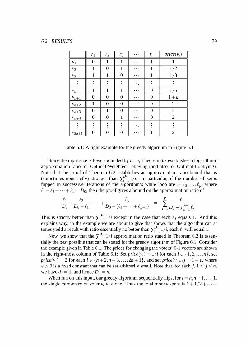
6.2. RESULTS 79
r1 r2 r3 · · · rn price(vi)
v1 0 1 1 · · · 1 1v2 1 0 1 · · · 1 1/2v3 1 1 0 · · · 1 1/3
......
......
. . ....
...vn 1 1 1 · · · 0 1/nvn+1 0 0 0 · · · 0 1+ εvn+2 1 0 0 · · · 0 2vn+3 0 1 0 · · · 0 2vn+4 0 0 1 · · · 0 2
......
......
. . ....
...v2n+1 0 0 0 · · · 1 2
Table 6.1: A tight example for the greedy algorithm in Figure6.1
Since the input size is lower-bounded bym·n, Theorem 6.2 establishes a logarithmicapproximation ratio for Optimal-Weighted-Lobbying (and also for Optimal-Lobbying).Note that the proof of Theorem 6.2 establishes an approximation ratio bound that is(sometimes nonstrictly) stronger than∑D0
i=11/i. In particular, if the number of zerosflipped in successive iterations of the algorithm’s while loop are`1, `2, . . . , `p, where`1+ `2+ · · ·+ `p = D0, then the proof gives a bound on the approximation ratio of
`1
D0+
`2
D0− `1+ · · ·+
`p
D0− (`1+ · · ·+ `p−1)=
p
∑j=1
` j
D0−∑ j−1k=1`k
.
This is strictly better than∑D0i=11/i except in the case that each` j equals 1. And this
explains why, in the example we are about to give that shows that the algorithm can attimes yield a result with ratio essentially no better than∑D0
i=11/i, each j will equal 1.Now, we show that the∑D0
i=11/i approximation ratio stated in Theorem 6.2 is essen-tially the best possible that can be stated for the greedy algorithm of Figure 6.1. Considerthe example given in Table 6.1. The prices for changing the voters’ 0-1 vectors are shownin the right-most column of Table 6.1: Setprice(vi) = 1/i for eachi ∈ {1,2, . . . ,n}, setprice(vi) = 2 for eachi ∈ {n+ 2,n+ 3, . . . ,2n+ 1}, and setprice(vn+1) = 1+ ε, whereε > 0 is a fixed constant that can be set arbitrarily small. Note that, for eachj, 1≤ j ≤ n,we haved j = 1, and henceD0 = n.
When run on this input, our greedy algorithm sequentially flips, fori = n,n−1, . . . ,1,the single zero-entry of votervi to a one. Thus the total money spent is 1+ 1/2+ · · ·+

80 CHAPTER 6. OPTIMAL LOBBYING
1/n= 1+1/2+ · · ·+1/D0. On the other hand, the optimal choice consists of influencingjust votervn+1 by flipping all ofvn+1’s entries to ones, which costs only 1+ ε.
6.3 Combinatorial Reverse Auctions
Combinatorial auctions are economically efficient allocations of wares in multiagent sys-tems. In combinatorial multi-unit auctions a seller would like to sell a set of differentitems, where he or she offers a different number of units of each item. A group of biddersgive bids, specifying how many units they want to buy from each item and which overallprice they would pay for it. The seller wants to maximize his revenue.
The opposite situation is, in which a buyer seeks to get a certain ammount of goodson minimal cost, this case is called a combinatorial reverseauction. This setting is notunnatural, it is indeed used in many market scenarios, for example, in procurement. Wenext give the formal definition stated as a minimization problem.
Name: Multi-Unit Combinatorial Reverse Auction.Instance: An m×n matrix L (whose rows represents the sellers, whose columns repre-
sent the items), with entriesλi, j ∈ N+ (representing the number of units of itemjthe buyer is willing to buy from selleri), where 1≤ i ≤mand 1≤ j ≤ n, the pricesof the bids(p1, p2, . . . , pm), wherepi ∈ Q+
0 for all 1≤ i ≤ m, and a target vectorx = (x1,x2, . . . ,xn), wherex j ∈N+ for all 1≤ j ≤ n.
Question: Find a minimum price subset of the rows, such that the auctioneer receives allof the units of items he or she is asking (i.e.,
minm
∑i=1
piyi such thatm
∑i=1
λi, jyi ≥ x j ,
whereyi ∈ {0,1} and 1≤ j ≤ n).
Sandholm et al. [SSGL02] proposed a greedy approximation algorithm for the Multi-Unit Combinatorial Reverse Auctions problem with the same logarithmic approximationratio as ours. Note, that the Optimal-Weighted-Lobbying problem is a special case of theMulti-Unit Combinatorial Reverse Auctions problem, with eachλi, j ∈ {0,1}.
6.4 Conclusions and Open Problems
Christian et al. [CFRS06] introduced the optimal lobbying problem and showed it com-plete for W[2], and so generally viewed as intractable in the sense of parameterized com-plexity. We proposed an efficient greedy algorithm for approximating the optimal solution

6.4. CONCLUSIONS AND OPEN PROBLEMS 81
of this problem, even if generalized by assigning prices to voters. The greedy algorithmachieves a logarithmic approximation ratio and we prove that that is essentially the bestapproximation ratio that can be proven for this algorithm. We also show the connectionbetween optimal lobbying and combinatorial reverse auctions introduced by Sandholm etal. [SSGL02].
We mention as an interesting open issue whether more elaborate algorithms canachieve better approximation ratios. Furthermore, it would be interesting to investigatemore general models of lobbying, for instance, when voters start with initial probabilitiesof voting for an issue and each voter has known costs for increasing their probabilitiesof voting according “The Lobby’s” agenda by each of a finite set of increments. Alsoother evaluation criteria could be considered, such as winning majority, where the aver-age probability of all the voters for an issue is above a predefined threshold.
A further direction for future work could be the investigation of combinatorial auctionsand reverse auctions, with respect to parameterized complexity.

82 CHAPTER 6. OPTIMAL LOBBYING

Chapter 7
Junta Distributions for SAT
This chapter is motivated by the notion of “frequently self-knowingly correct algorithms,”which was proposed by Homan and Hemaspaandra [HHb] in their work on how to fre-quently find winners of Dodgson elections [Dod76].
7.1 A Motivation: How to Find Dodgson Winners Fre-quently
Recall the definition of Dodgson’s voting system: If(C,V) is an election andc is somedesignated candidate inC, we call (C,V,c) a Dodgson triple. An election is won bythose candidates who are “closest” to being a Condorcet winner. More precisely, given aDodgson election(C,V), every candidatec in C is assigned a score, which is denoted byDodgsonScore(C,V,c), and is defined to be the smallest number of sequential exchangesof adjacent preferences in the voters’ preference orders needed to makec a Condorcetwinner with respect to the resulting preference orders. Whoever has the lowest Dodgsonscore wins.
The problem Dodgson-Winner is defined as follows:
Name: Dodgson-Winner.Instance: An election(C,V) and a designated candidatec in C.Question: Is c a Dodgson winner in(C,V)?
The search version of this decision problem can easily be stated. As mentioned earlier,Hemaspaandra, Hemaspaandra, and Rothe [HHR97] have shown that determining theDodgson winner is PNP
‖ -complete.
83

84 CHAPTER 7. JUNTA DISTRIBUTIONS FOR SAT
It certainly is not desirable to have an election system whose winner problem is hard,as only systems that can be evaluated efficiently are actually used in practice. Fortu-nately, there are a number of positive results on Dodgson elections and related systems aswell. In particular, Bartholdi, Tovey, and Trick [BTT89b] proved that for elections with abounded number of candidates or voters Dodgson winners are asymptotically easy to de-termine. Fishburn [Fis77] proposed a “homogeneous” variant of Dodgson elections thatRothe, Spakowski, and Vogel [RSV03] proved to have a polynomial-time winner prob-lem. McCabe-Dansted, Pritchard, and Slinko [MPS] proposeda scheme (called DodgsonQuick) that approximates Dodgson’s rule with an exponentially fast convergence. Homanand Hemaspaandra ([HHa], see also McCabe-Dansted, Pritchard, and Slinko [MPS]) pro-posed a greedy heuristic that finds Dodgson winners with a “guaranteed high frequencyof success.” To capture a strengthened version of this property formally, they introducedthe notion of a “frequently self-knowingly correct algorithm”, and they noted [HHa]:
“The closest related concepts [. . .] are probably those involving proofs to beverified, such as NP certificates and the proofs in interactive proof systems.”
This statement notwithstanding, we show how average-case polynomial time relatesto the notion of frequently self-knowingly correct algorithm.
7.2 Average-Case Complexity Theory
To prove a problem NP-hard is a common method of showing its computational in-tractability as described in Chapter 2. Many NP-hard problems, however, are eminentlyimportant in practice, which is why various approaches to coping with NP-hardness havebeen proposed, including approximation algorithms (see, Chapter 6), parameterized com-plexity (see, Section 2.3), heuristics/algorithms that are always efficient (i.e., polynomial-time) albeit not always correct (for example, the class P-close [Sch86]), algorithms thatare always correct albeit not always efficient (for example,the class APT [MP79]), etc.A particularly interesting approach is to show that some NP-hard problems can be solvedefficiently on the average.
The theory of average-case complexity was initiated by Levin [Lev86]. A problem’saverage-case complexity can be viewed as a more significant measure than its worst-casecomplexity in many cases, for example in cryptographic applications. We here followGoldreich’s presentation [Gol97]. Another excellent introduction to this theory is that ofWang [Wan97].
Intuitively, Levin observed that many hard problems—including those that are NP-hard in the traditional worst-case complexity model—mightnonetheless be easy to solve“on the average,” i.e., for “most” inputs or for “most practically relevant” inputs. He
7.2. AVERAGE-CASE COMPLEXITY THEORY 85
proposed to define the complexity of problems with respect tosome suitable distributionon the input strings.
We now define the notion of a distributional problem and the complexity class AvgP.In this chapter, we consider two heuristic algorithms: the algorithm Greedy-Winner in-tends to solve the decision problem Dodgson-Winner, and thealgorithm Greedy-Scoreintends to compute the Dodgson score of some given candidate. Both heuristics workwell sufficiently often, provided that the number of voters greatly exceeds the number ofcandidates.
Here, we define only distributional search problems; the definition of distributionaldecision problems is analogous.
Definition 7.1 ([Lev86], see also [Gol97, Wan97]). 1. A distribution function µ :Σ∗→ [0,1] is a nondecreasing function from strings to the unit interval that con-verges to one (i.e.,µ(0) ≥ 0, µ(x) ≤ µ(y) for each x< y, andlimx→∞ µ(x) = 1).The density function associated withµ is defined byµ ′(0) = µ(0) and µ ′(x) =µ(x)− µ(x−1) for each x> 0. That is, each string x gets weightµ ′(x) with thisdistribution.
2. A distributional (search) problemis a pair ( f ,µ), where f : Σ∗→ Σ∗ is a functionandµ : Σ∗→ [0,1] is a distribution function.
3. A function t: Σ∗→ N is polynomial on the average with respect to some distribu-tion µ if there exists a constantε > 0 such that
∑x∈Σ∗
µ ′(x) ·t(x)ε
|x|< ∞.
4. The classAvgP consists of all distributional problems( f ,µ) for which there existsan algorithmA computing f such that the running time ofA is polynomial on theaverage with respect to the distributionµ.
In Section 7.4, we will focus on the standard uniform distribution µ on Σ∗, which isdefined by
µ ′(x) =1
|x|(|x|+1)2|x|.
That is, we first choose an input sizen at random with probability 1/(n(n+1)), and thenwe choose an input string of that sizen uniformly at random.
In Section 7.4, we we will make use of polynomial-time benignalgorithm schemes.This notion was introduced by Impagliazzo [Imp95] to provide an alternative view on the

86 CHAPTER 7. JUNTA DISTRIBUTIONS FOR SAT
definition of Levin’s class AvgP (average polynomial time, see [Lev86]). Impagliazzo de-fines AvgP to be the class of distributional problems( f ,µn) such that there is an algorithmcomputingf in polynomial time on the average with respect to the input ensembleµn.
We in this chapter use the following notation. For any distribution µ and for eachn ∈ N let µn be the restriction ofµ to strings of length exactlyn, and letµ≤n be therestriction ofµ to strings of length at mostn. (When discussing benign algorithms, thelength-0 stringε is routinely completely excluded from the probability distribution—itis by convention given weight zero—and so for such cases, e.g., Definition 7.2, the “foreachn∈N” should be viewed as changed to saying “for eachn∈ N+.”)
Definition 7.2 ([Imp95]). 1. An algorithm computes a function f withbenign faultsifit either outputs an element of the image of f or “?,” and if it outputs anything otherthan?, it is correct.
2. Let µ be a distribution onΣ∗. A polynomial-time benign algorithm schemefor afunction f onµ is an algorithmA (x,δ ) such that:
(a) A runs in time polynomial in|x| and1/δ .
(b) A computes f with benign faults.
(c) For eachδ , 0 < δ < 1, and for each n∈N+,
Probµ≤n[A (x,δ ) = ?]≤ δ .
The following theorem gives Impagliazzo’s characterization of AvgP.
Theorem 7.1([Imp95]). A problem f onµ is in AvgP if and only if it has a polynomial-time benign algorithm scheme onµ.
7.3 Frequently Self-Knowingly Correct Algorithms
Homan and Hemaspaandra [HHa] proposed the following definition of a new type ofalgorithm to capture the notion of “guaranteed high successfrequency” formally.
Definition 7.3 ([HHa]). 1. Let f : S→ T be a function, where S and T are sets. Wesay an algorithmA : S→ T×{“definitely”, “maybe” } is self-knowingly correctfor f if, for each s∈ S and t∈ T, wheneverA on input s outputs(t, “definitely” )then f(s) = t.
2. An algorithmA that is self-knowingly correct for g: Σ∗→T is said to befrequentlyself-knowingly correct forg if
limn→∞
‖{x∈ Σn |A(x) ∈ T×{“maybe”}}‖‖Σn‖
= 0.

7.3. FREQUENTLY SELF-KNOWINGLY CORRECT ALGORITHMS 87
In their paper [HHa], Homan and Hemaspaandra present two frequently self-knowingly correct polynomial-time algorithms, which theycall Greedy-Score andGreedy-Winner. Since Greedy-Winner can easily be reduced to Greedy-Score, we fo-cus on Greedy-Score only and briefly describe the intuition behind this algorithm; for fulldetail, we refer to [HHa]. (But both heuristics work well tremendously often—in a formalsense of the notion—provided that the number of voters greatly exceeds the number ofcandidates.)
Given a Dodgson triple(C,V,c), Greedy-Score determines the Dodgson score ofcwith respect to the given election(C,V). We will see that there are Dodgson triples(C,V,c) for which this problem is particularly easy to solve.
For anyd ∈C−{c}, let Deficit[d] be the number of votesc needs to gain in order tohave more votes thand in a pairwise contest betweenc andd.
Definition 7.4. Any Dodgson triple(C,V,c) is said to benice if and only if for eachcandidate d∈C−{c}, there are at leastDeficit[d] votes for which candidate c is exactlyone position below candidate d.
Given a Dodgson triple(C,V,c), the algorithm Greedy-Score works as follows:
1. For each candidated ∈C−{c}, determine Deficit[d].
2. If (C,V,c) is not nice then output(“anything”,“maybe”); otherwise, if(C,V,c) isnice then output
(∑d∈C−{c}Deficit[d], “definitely”).
Note that, for nice Dodgson triples, we have
DodgsonScore(C,V,c) = ∑d∈C−{c}
Deficit[d],
It is easy to see that Greedy-Score is a self-knowingly correct polynomial-timebounded algorithm. To show that it is evenfrequentlyself-knowingly correct, Homanand Hemaspaandra prove the following lemma. Their proof uses a variant of Chernoffbounds which we introduce next.
Lemma 7.1(Lemma 11.9 of [Pap95]). Let x1,x2, . . . ,xn be independent random variableswith xi ∈ {0,1} for all i, 1≤ i ≤ n, and let X= ∑n
i=1xi . Each variable with value1 or 0has probability p or1− p, respectively. Then for all0≤ θ ≤ 1,
Prob[X ≥ (1+θ)pn]≤ e−θ23 pn.

88 CHAPTER 7. JUNTA DISTRIBUTIONS FOR SAT
Lemma 7.2(Thm. 4.1.3 of [HHa]). Let (C,V,c) be a given Dodgson triple, where‖V‖=n and‖C‖ = m, chosen uniformly at random among all such Dodgson elections. The
probability that(C,V,c) is not nice is at most2(m−1)e−n
8m2 .
Proof. Suppose that(C,V,c) is not nice. Then, for somed ∈V−{c},
‖{i ∈ {1, . . .n}|c<vi d}‖−n2≥ ‖{i ∈ {1, . . .n}|c≺vi d}‖.
This is true only if, for somed ∈V−{c}, at least one of (7.3.1) and (7.3.3) is true, where
||{i ∈ {1, . . .n}|c <vi d}||−n2
(7.3.1)
≥14·
nm
,(7.3.2)
||{i ∈ {1, . . .n}|c≺vi d}||(7.3.3)
≤34·
nm
.(7.3.4)
Using Chernoff bounds (see Lemma 7.1), it is easy to prove that the probability forboth the events (7.3.1) and (7.3.3) are exponentially smallin n
24m2 . Here, the fact is usedthat for arbitrary fixed candidatesa andb, for some random votevi , Prob[a <vi b] = 1/2and Prob[a≺vi b] = 1/m.
Summing over all candidatesd ∈C−{c}, we obtain that the probability that(C,V,c)
is not nice, is≤ 2(m−1)e−n
24m2 . ❑
Homan and Hemaspaandra [HHa] show that the heuristic Greedy-Winner, which isbased on Greedy-Score and which solves the winner problem for Dodgson elections, alsois a frequently self-knowingly correct polynomial-time algorithm. This result is statedformally below.
Theorem 7.2(Thm. 4.4.2 of [HHa]). For all m,n∈ N+, the probability that a Dodgsonelection(C,V) selected uniformly at random from all Dodgson elections having m can-didates and n votes (i.e., all(m!)n Dodgson elections having m candidates and n voteshave the same likelihood of being selected) has the propertythat there exists at least onecandidate c such that Greedy-Winner on input(C,V,c) outputs “maybe” as its second
output component is less than2(m2−m)e−n
8m2 .
7.4 AvgP vs. Frequently Self-Knowingly Correct Algo-rithms
Our main result in this section relates polynomial-time benign algorithm schemes to fre-quently self-knowingly correct algorithms. We show that every distributional problem

7.4. AVGP VS. FREQUENTLY SELF-KNOWINGLY CORRECT ALGORITHMS 89
that has a polynomial-time benign algorithm scheme with respect to the uniform distri-bution must also have a frequently self-knowingly correct polynomial-time algorithm. Itfollows that all uniformly distributed AvgP problems have afrequently self-knowinglycorrect polynomial-time algorithm.
Theorem 7.3.Suppose thatA (x,δ ) is a polynomial-time benign algorithm scheme for adistributional problem f onµ (the standard uniform distribution, see Section 7.2). Thenthere is a frequently self-knowingly correct polynomial-time algorithmA
′ for f .
Proof. For eachn∈N, let δ (n) = 1/(n+1)3. Define algorithmA ′ as follows:
1. On inputx∈ Σ∗, simulateA (x,δ (|x|)).
2. If A (x,δ (|x|)) outputs ?, then output(anything, “maybe”).
3. If A (x,δ (|x|)) outputsy∈ T, wherey 6=?, then output(y, “definitely” ).
By Definition 7.2, of “polynomial-time benign algorithm scheme,” algorithmA′ runs in
polynomial time. It remains to show thatA ′ is frequently self-knowingly correct.Fix an arbitraryn ∈ N+. Now, we must be careful regarding the fact that Impagli-
azzo’s definition of benign algorithm schemes and its “δ ” guarantees are all with regardto drawing not over inputs of a given length (which is what we wish to consider) butrather regarding drawing from inputsup to and includinga given length. Thus, there issome danger that even if a benign algorithm performs well when its length parameter isn (meaning related to strings of length up to and includingn), that such a “good” errorfrequency might be due not to goodness at lengthn but rather to goodness at lengthsn−1,n−2, and so on. However, if one looks carefully at the relative weights of the differentlengths this is at most a quadratically weighted effect (that is, the distribution’s probabilityweight at lengthn is just quadratically less than the weight summed over all lengths lessthann), and so our choice ofδ (n) = 1/(n+1)3 is enough to overcome this.
Let us now handle that rigorously. Recall thatn is fixed and arbitrary. Let us set theconstant (for fixedn) δ ′ to be 1/(n+1)3. So, clearly
Probµ≤n[A (x,δ ′) = ?] =
∑n−1i=1 1/(i(i +1))
∑ni=11/(i(i +1))
Probµ≤n−1[A (x,δ ′) = ?]+1/(n(n+1))
∑ni=11/(i(i +1))
Probµn[A (x,δ ′) = ?].
SinceA is a benign algorithm scheme, Probµ≤n[A (x,δ ′) = ?] ≤ δ ′. So, combining thisand the above equality, and solving for Probµn[A (x,δ ′) = ?], we have
Probµn[A (x,δ ′) = ?]≤
∑ni=11/(i(i +1))
1/(n(n+1))
(
δ ′− ∑n−1i=1 1/(i(i +1))
∑ni=11/(i(i +1))
Probµ≤n−1[A (x,δ ′) = ?]
)
.

90 CHAPTER 7. JUNTA DISTRIBUTIONS FOR SAT
And so, clearly, Probµn[A (x,δ ′) = ?]≤ n(n+1)δ ′ = n(n+1)/(n+1)3. So
limn→∞
‖{x∈ Σn |A ′(x) ∈ T×{“maybe”}}‖‖Σn‖
= 0,
which completes the proof. ❑
Corollary 7.1. Every distributional problem that under the standard uniform distributionis in AvgPhas a frequently self-knowingly correct polynomial-time algorithm.
Proof. Impagliazzo proved that any distributional problem on input ensembleµn is inAvgP if and only if it has a polynomial-time benign algorithmscheme; see Proposition 2in [Imp95]. The claim now follows from Theorem 7.3. ❑
It is easy to see that the converse implication of that in Corollary 7.1 is not true.
Proposition 7.1. There exist (distributional) problems with a frequently self-knowinglycorrect polynomial-time algorithm that are not inAvgP under the standard uniform dis-tribution.
Proof. For instance, one can define a problem that consists only of strings in {0}∗
encoding the halting problem. This problem is clearly not inAvgP, yet it is frequentlyself-knowingly correct. ❑
7.5 A Basic Junta Distribution for SAT
Procaccia and Rosenschein [PR07] introduced “junta distributions” in their study of NP-hard manipulation problems for elections. The goal of a junta is to be such a hard dis-tribution (that is, to focus so much weight on hard instances) that if a problem is easyrelative to a junta then it will be easy relative to any reasonable distribution (such as theuniform distribution).
Regarding Procaccia and Rosenschein’s notion of juntas, they state three “basic” con-ditions for a junta, and then give two additional ones that are tailored specifically to theneeds of NP-hard voting manipulation problems. They state their hope that their schemewill extend more generally, using the three basic conditions and potentially additionalconditions, to other mechanism problems. We will show that the three basic conditionsfor a junta are sufficiently weak that one can construct a junta relative to which the stan-dard NP-complete problem SAT—and a similar attack can be carried out on a wide range
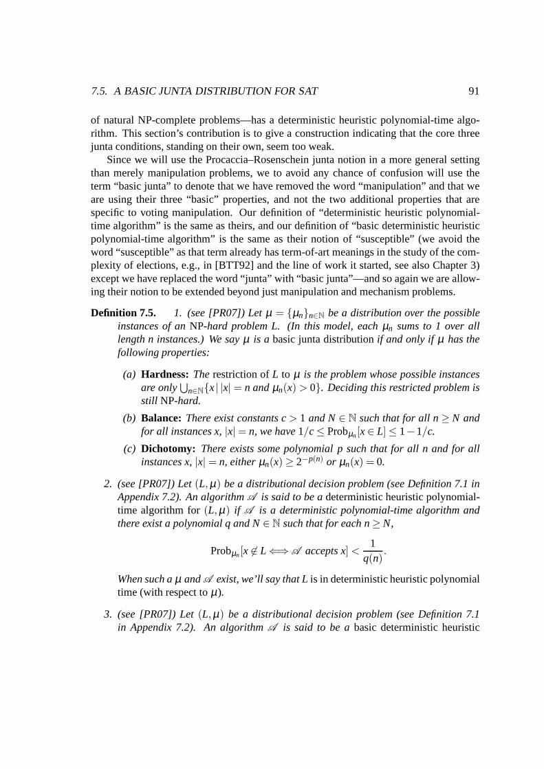
7.5. A BASIC JUNTA DISTRIBUTION FOR SAT 91
of natural NP-complete problems—has a deterministic heuristic polynomial-time algo-rithm. This section’s contribution is to give a construction indicating that the core threejunta conditions, standing on their own, seem too weak.
Since we will use the Procaccia–Rosenschein junta notion ina more general settingthan merely manipulation problems, we to avoid any chance ofconfusion will use theterm “basic junta” to denote that we have removed the word “manipulation” and that weare using their three “basic” properties, and not the two additional properties that arespecific to voting manipulation. Our definition of “deterministic heuristic polynomial-time algorithm” is the same as theirs, and our definition of “basic deterministic heuristicpolynomial-time algorithm” is the same as their notion of “susceptible” (we avoid theword “susceptible” as that term already has term-of-art meanings in the study of the com-plexity of elections, e.g., in [BTT92] and the line of work itstarted, see also Chapter 3)except we have replaced the word “junta” with “basic junta”—and so again we are allow-ing their notion to be extended beyond just manipulation andmechanism problems.
Definition 7.5. 1. (see [PR07]) Letµ = {µn}n∈N be a distribution over the possibleinstances of anNP-hard problem L. (In this model, eachµn sums to 1 over alllength n instances.) We sayµ is a basic junta distributionif and only if µ has thefollowing properties:
(a) Hardness: Therestriction ofL to µ is the problem whose possible instancesare only
⋃
n∈N{x| |x| = n andµn(x) > 0}. Deciding this restricted problem isstill NP-hard.
(b) Balance: There exist constants c> 1 and N∈ N such that for all n≥ N andfor all instances x,|x|= n, we have1/c≤ Probµn[x∈ L]≤ 1−1/c.
(c) Dichotomy: There exists some polynomial p such that for all n and for allinstances x,|x|= n, eitherµn(x)≥ 2−p(n) or µn(x) = 0.
2. (see [PR07]) Let(L,µ) be a distributional decision problem (see Definition 7.1 inAppendix 7.2). An algorithmA is said to be adeterministic heuristic polynomial-time algorithm for(L,µ) if A is a deterministic polynomial-time algorithm andthere exist a polynomial q and N∈N such that for each n≥N,
Probµn[x 6∈ L⇐⇒A accepts x] <1
q(n).
When such aµ andA exist, we’ll say that Lis in deterministic heuristic polynomialtime (with respect toµ).
3. (see [PR07]) Let(L,µ) be a distributional decision problem (see Definition 7.1in Appendix 7.2). An algorithmA is said to be abasic deterministic heuristic

92 CHAPTER 7. JUNTA DISTRIBUTIONS FOR SAT
polynomial-time algorithm for(L,µ) if µ is a basic junta distribution (for L),Ais a deterministic polynomial-time algorithm, and there exist a polynomial q andN ∈N such that for each n≥N,
Probµn[x 6∈ L⇐⇒A accepts x] <1
q(n).
When such aµ and A exist, we’ll say that Lis in basic deterministic heuristicpolynomial time (with respect toµ).
We now explore their notion of deterministic heuristic polynomial time and their no-tion of junta, both however viewed for general NP problems and using the “basic” threeconditions. We will note that the notion in such a setting is in some senses not restrictiveenough and in other senses is too restrictive. Let us start with the former. We need adefinition.
Definition 7.6. We will say that a set L iswell-pierced(respectively,uniquely well-pierced) if there exist sets Pos∈ P and Neg∈ P such that Pos⊆ L, Neg⊆ L, and thereis some N∈N such that at each length n≥N, each of Pos and Neg has at least one stringat length n (respectively, each of Pos and Neg has exactly onestring at length n).
Each uniquely well-pierced set is well-pierced. Note that,under quite natural encod-ings, such NP-complete sets as, for example, SAT certainly are well-pierced and uniquelywell-pierced. (All this says is that, except for a finite number of exceptional lengths,there is one special string at each length that can easily, uniformly be recognized as inthe set and one that can easily, uniformly be recognized as not in the set.) Indeed, underquite natural encodings, undecidable problems such as the halting problem are uniquelywell-pierced.
Recall that juntas are defined in relation to an infinite list of distributions, one perlength (soµ = {µn}n∈N). The Procaccia and Rosenschein definition of junta does notexplicitly put computability or uniformity requirements on such distributions in the def-inition of junta, but it is useful to be able to make claims about that. So let us say thatsuch a distribution isuniformly computable in polynomial time(respectively, isuniformlycomputable in exponential time) if there is a polynomial-time function (respectively, anexponential-time function)f such that for eachi and eachx, f (i,x) outputs the value ofµi(x) (say, as a rational number—if a distribution takes on other values, it simply will notbe able to satisfy our notion of good uniform time).
Theorem 7.4. Let A be anyNP-hard set that is well-pierced. Then there exists a basicjunta distribution relative to which A has a basic deterministic heuristic polynomial-timealgorithm (indeed, it even has a basic deterministic heuristic polynomial-time algorithm

7.5. A BASIC JUNTA DISTRIBUTION FOR SAT 93
whose error weight is bounded not merely by1/poly as the definition requires, but is evenbounded by1/2n2−n). Furthermore, the junta is uniformly computable in exponentialtime, and if we in addition assume that A is uniquely well-pierced, the junta is uniformlycomputable in polynomial time.
It follows that, under quite natural encodings, almost any natural set is in basic deter-ministic heuristic polynomial time. For example, SAT is andthe halting problem is, bothunder natural encodings. All it takes is for the given set to have at all but a finite numberof lengths at least one element each that are uniformly easily recognizable as being in andout of the set.
Proof. Let A be well-pierced. So there exists anN, and setsPosandNeg, that satisfythe definition of well-pierced. For eachn≥ N, let Pos(n) denote the lexicographicallysmallest lengthn string inPosand letNeg(n) denote the lexicographically smallest lengthn string inNeg.
Define the distributionν = {νn}n∈N as follows:
1. For each lengthn≥ N, put weight 1/2n2on all lengthn strings other thanPos(n)
andNeg(n), and put weight12
(
1− 2n−22n2
)
on each ofPos(n) andNeg(n).
2. For each lengthn < N, let νn be the uniform distribution over that length, i.e., eachlengthn string has weight 1/2n.
We now show thatν is a basic junta distribution.
1. Hardness: Since⋃
n∈N{x| |x| = n andνn(x) > 0} equalsΣ∗, the restriction ofA toν equalsA, and so is still NP-hard.
2. Balance: Since for each lengthn ≥ N both Pos(n) ∈ A and Neg(n) 6∈ A havealmost half of the probability weight of all lengthn strings (namely, each has12
(
1− 2n−22n2
)
), ν is balanced.
3. Dichotomy: Since for alln≥ N and for allx, |x| = n, we haveνn(x) ≥ 2−n2, and
for all n < N and for allx, |x|= n, we haveνn(x)≥ 2−n, dichotomy is satisfied.
Note that the junta is uniformly computable in exponential time, and ifA is uniquelywell-pierced then the junta is uniformly computable in polynomial time.
Our basic deterministic heuristic polynomial-time algorithm for (A,ν) works as fol-lows: On inputs that are aPos(n), it accepts; on inputs that are aNeg(n), it rejects; and onevery other input, it (for specificity, though it does not matter) accepts.
For eachn≥N, the error probability of this algorithm on inputs of lengthn is at most(2n−2)/2n2
≤ 1/2n2−n. ❑

94 CHAPTER 7. JUNTA DISTRIBUTIONS FOR SAT
In the proof we achieve the error bound 1/2n2−n stated in Theorem 7.4. However, thisbound can easily be strengthened to 1/2nk−n, for each fixed constantk, by altering theproof. Note that the altered algorithm will depend onk.
Loosely put, the above result says that the basic junta conditions are in some waysoverinclusive. We also note that the definition of junta, andthe issue of when we willhave a basic deterministic heuristic polynomial-time algorithm, are exceedingly sensitiveto details of encoding.1 We mention quickly two such effects, one that indirectly suggestsoverinclusiveness and one that suggests underinclusiveness.
As to the former, note thateveryNP-hard set is≤pm-reducible to a set that is in basic
deterministic heuristic polynomial time. This applies even to undecidable NP-hard sets,such as SAT⊕HP =de f {0x| x ∈ SAT} ∪ {1y| y ∈ HP}, where HP denotes the haltingproblem. The proof is nearly immediate. Given an NP-hard setA (over some alphabetΣthat has cardinality at least two, and w.l.o.g. we assume that 0 and 1 are letters ofΣ), notethatA≤p
m-reduces to the setA′ = {00x|x∈ Σ∗}∪{1x1|x|2+2 |x∈ A}, and thatA′ is easily
seen to be in basic deterministic heuristic polynomial time(indeed, with error bound notjust 1/polybut even 1/exponential), in particular via the basic junta (relative toA′) that isthe uniform distribution.
Regarding underinclusiveness, note that under the definition of basic junta, no setthat at an infinite number of lengths either has all strings orhas no strings can have abasic deterministic heuristic polynomial-time algorithm, since for such sets the balancecondition of the notion of a basic junta can never be satisfied. It follows easily that thenotion of having a basic deterministic heuristic polynomial-time algorithm is not evenclosed under polynomial-time isomorphisms.2
1In contrast, the “ε” exponent and|x| denominator (see Definition 7.1 in Section 7.2) in Levin’s [Lev86]theory of AvgP, average-case polynomial-time, were precisely designed, in that different setting, to avoidsuch problems—problems that one gets by following the type of asymptotic focus on one length at a timethat the Procaccia and Rosenschein model adopts. On the other hand, even Levin’s theory has many sub-tleties and downsides, and to this day has not found anythingresembling the type of widespread applicabilityof NP-completeness theory; see any of the many surveys on that topic.
2To be extremely concrete, the NP-complete setB = {00x| x ∈ Σ∗}∪ {1x1|x|2+2 | x ∈ SAT} is (as per
the above) easily seen to be in basic deterministic heuristic polynomial time, but the NP-complete setB′ = {xx|x∈ SAT}, though it is by standard techniques polynomial-time isomorphic toB (see [BH77]), isnot in basic deterministic heuristic polynomial time. If the reader wonders why we did not simply use twoP sets, the reason is, under the Procaccia–Rosenschein definition, one needs NP-hardness to have a junta,and one needs a junta to put something in deterministic heuristic polynomial time.
Bibliography
[Arr63] K. Arrow. Social Choice and Individual Values. John Wiley and Sons, 1951(revised edition 1963).
[BEH+ar] D. Baumeister, G. Erdelyi, E. Hemaspaandra, L. Hemaspaandra, andJ. Rothe. Approval voting. In J. Laslier and R. Sanver, editors, ApprovalVoting. Springer-Verlag, To Appear.
[BF78] S. Brams and P. Fishburn. Approval voting.American Political ScienceReview, 72(3):831–847, 1978.
[BF83] S. Brams and P. Fishburn.Approval Voting. Birkhauser, Boston, 1983.
[BF02] S. Brams and P. Fishburn. Voting procedures. In K. Arrow, A. Sen, andK. Suzumura, editors,Handbook of Social Choice and Welfare, volume 1,pages 173–236. North-Holland, 2002.
[BH77] L. Berman and J. Hartmanis. On isomorphisms and density of NP and othercomplete sets.SIAM Journal on Computing, 6(2):305–322, 1977.
[BK98] S. Brams and D. Kilgour. Fallback bargaining. Technical report, 1998.
[BL05] S. Bouveret and J. Lang. Efficiency and envy-freenessin fair division ofindivisible goods: Logical representation and complexity. In Proceedingsof the 19th International Joint Conference on Artificial Intelligence, pages935–940. Professional Book Center, July/August 2005.
[Bla58] D. Black. The Theory of Committees and Elections. Cambridge UniversityPress, 1958.
[BS] S. Brams and R. Sanver. Voting systems that combine approval and prefer-ence. In S. Brams, W. Gehrlein, and F. Roberts, editors,The Mathematicsof Preference, Choice, and Order: Essays in Honor of Peter C.Fishburn.Springer. To appear.
95

96 BIBLIOGRAPHY
[BS06] S. Brams and R. Sanver. Critical strategies under approval voting: Who getsruled in and ruled out.Electoral Studies, 25(2):287–305, 2006.
[BTT89a] J. Bartholdi III, C. Tovey, and M. Trick. The computational difficulty ofmanipulating an election.Social Choice and Welfare, 6(3):227–241, 1989.
[BTT89b] J. Bartholdi III, C. Tovey, and M. Trick. Voting schemes for which it can bedifficult to tell who won the election.Social Choice and Welfare, 6(2):157–165, 1989.
[BTT92] J. Bartholdi III, C. Tovey, and M. Trick. How hard is it to control an election?Mathematical Comput. Modelling, 16(8/9):27–40, 1992.
[BU08] N. Betzler and J. Uhlmann. Parameterized complexityof candidate controlin elections and related digraph problems. InProceedings of the 2nd AnnualInternational Conference on Combinatorial Optimization and Applications,pages 43–53. Springer-VerlagLecture Notes in Computer Science #5165,August 2008.
[CCDF97] L. Cai, J. Chen, R. G. Downey, and M. R. Fellows. On the parameterizedcomplexity of short computation and factorization.Archive for Mathemati-cal Logic, 36(4-5):321–337, 1997.
[CELM07] Y. Chevaleyre, U. Endriss, J. Lang, and N. Maudet. Ashort introductionto computational social choice. InProceedings of the 33rd Conference onCurrent Trends in Theory and Practice of Computer Science, pages 51–69.Springer-VerlagLecture Notes in Computer Science#4362, January 2007.
[Ces03] M. Cesati. The turing way to parameterized complexity. Journal of Com-puter and System Sciences, 67(4):654 – 685, 2003.
[CFRS06] R. Christian, M. Fellows, F. Rosamond, and A. Slinko. On complexity oflobbying in multiple referenda. In U. Endriss and J. Lang, editors, 1st In-ternational Workshop on Computational Social Choice (COMSOC 2006),pages 87–96 (workshop notes). Universiteit van Amsterdam,December2006.
[CLRS01] T. Cormen, C. Leiserson, R. Rivest, and C. Stein.Introduction to Algo-rithms. MIT Press and McGraw-Hill, second edition, 2001.
[Con85] J.-A.-N. de Caritat, Marquis de Condorcet. Essai sur l’application del’analyse a la probabilite des decisions rendues a la pluralite des voix. 1785.

BIBLIOGRAPHY 97
Facsimile reprint of original published in Paris, 1972, by the ImprimerieRoyale. English translation appears in I. McLean and A. Urken, Classics ofSocial Choice, University of Michigan Press, 1995, pages 91–112.
[Coo71] S. Cook. The complexity of theorem-proving procedures. InProceedingsof the 3rd ACM Symposium on Theory of Computing, pages 151–158. ACMPress, 1971.
[DF95] R. Downey and M. Fellows. Fixed-parameter tractability and completenessii: On completeness for w[1].Theoretical Computer Science, 141(1-2):109–131, April 1995.
[DF99] R. Downey and M. Fellows.Parameterized Complexity. Springer-Verlag,Berlin, Heidelberg, New York, 1999.
[Die05] R. Diestel. Graph Theory. Graduate Texts in Mathematics, Volume 173.Springer-Verlag, Berlin, Heidelberg, New York, 2005.
[DKNS01] C. Dwork, R. Kumar, M. Naor, and D. Sivakumar. Rank aggregation meth-ods for the web. InProceedings of the 10th International World Wide WebConference, pages 613–622. ACM Press, 2001.
[Dod76] C. Dodgson. A method of taking votes on more than two issues. Pamphletprinted by the Clarendon Press, Oxford, and headed “not yet published” (seethe discussions in [MU95, Bla58], both of which reprint thispaper), 1876.
[DS00] J. Duggan and T. Schwartz. Strategic manipulabilitywithout resolutenessor shared beliefs: Gibbard–Satterthwaite generalized.Social Choice andWelfare, 17(1):85–93, 2000.
[EHRS07a] G. Erdelyi, L. Hemaspaandra, J. Rothe, and H. Spakowski. On approximat-ing optimal weighted lobbying, and frequency of correctness versus average-case polynomial time. InProceedings of the 16th International Symposiumon Fundamentals of Computation Theory, pages 300–311. Springer-VerlagLecture Notes in Computer Science #4639, August 2007.
[EHRS07b] G. Erdelyi, L. Hemaspaandra, J. Rothe, and H. Spakowski. On approximat-ing optimal weighted lobbying, and frequency of correctness versus average-case polynomial time. Technical Report TR-914, Departmentof ComputerScience, University of Rochester, Rochester, NY, March 2007.
[EKM07] P. Everaere, S. Konieczny, and P. Marquis. The strategy-proofness landscapeof merging.Journal of Artificial Intelligence Research, 28:49–105, 2007.

98 BIBLIOGRAPHY
[ENR08a] G. Erdelyi, M. Nowak, and J. Rothe. Sincere-strategy preference-basedapproval voting broadly resists control. InProceedings of the 33rd Inter-national Symposium on Mathematical Foundations of Computer Science,pages 311–322. Springer-VerlagLecture Notes in Computer Science #5162,August 2008.
[ENR08b] G. Erdelyi, M. Nowak, and J. Rothe. Sincere-strategy preference-based ap-proval voting fully resists constructive control and broadly resists destructivecontrol. Technical Report arXiv:0806.0535v4 [cs.GT], ACMComputingResearch Repository (CoRR), June 2008. Revised, September2008.
[ER93] E. Ephrati and J. Rosenschein. Multi-agent planningas a dynamic search forsocial consensus. InProceedings of the 13th International Joint Conferenceon Artificial Intelligence, pages 423–429. Morgan Kaufmann, 1993.
[Fal08] P. Faliszewski. Nonuniform bribery. InProceedings of the 7th Interna-tional Joint Conference on Autonomous Agents and Multiagent Systems,pages 1569–1572. ACM Press, May 2008.
[FG06] J. Flum and M. Grohe.Parameterized Complexity Theory. EATCS Texts inTheoretical Computer Science. Springer-Verlag, Berlin, Heidelberg, 2006.
[FHH06a] P. Faliszewski, E. Hemaspaandra, and L. Hemaspaandra. The complexity ofbribery in elections. InProc. AAAI’06, pages 641–646. AAAI Press, 2006.
[FHH06b] P. Faliszewski, E. Hemaspaandra, and L. Hemaspaandra. The complexityof bribery in elections. InProceedings of the 21st National Conference onArtificial Intelligence, pages 641–646. AAAI Press, July 2006.
[FHH06c] P. Faliszewski, E. Hemaspaandra, and L. Hemaspaandra. How hard isbribery in elections? Technical Report TR-895, Departmentof ComputerScience, University of Rochester, Rochester, NY, April 2006. Revised,September 2006.
[FHHR] P. Faliszewski, E. Hemaspaandra, L. Hemaspaandra, and J. Rothe. Aricher understanding of the complexity of election systems. In S. Ravi andS. Shukla, editors,Fundamental Problems in Computing: Essays in Honorof Professor Daniel J. Rosenkrantz. Springer. To appear.
[FHHR07a] P. Faliszewski, E. Hemaspaandra, L. Hemaspaandra, and J. Rothe. Llulland Copeland voting broadly resist bribery and control. InProceedings ofthe 22nd AAAI Conference on Artificial Intelligence, pages 724–730. AAAIPress, July 2007.

BIBLIOGRAPHY 99
[FHHR07b] P. Faliszewski, E. Hemaspaandra, L. Hemaspaandra, and J. Rothe. Llull andCopeland voting broadly resist bribery and control. InProc. AAAI’07, pages724–730. AAAI Press, 2007.
[FHHR08a] P. Faliszewski, E. Hemaspaandra, L. Hemaspaandra, and J. Rothe. Copelandvoting fully resists constructive control. InProceedings of the 4th Interna-tional Conference on Algorithmic Aspects in Information and Management,pages 165–176. Springer-VerlagLecture Notes in Computer Science #5034,June 2008.
[FHHR08b] P. Faliszewski, E. Hemaspaandra, L. Hemaspaandra, and J. Rothe. Copelandvoting fully resists constructive control. InProc. AAIM’08, pages 165–176.Springer-Verlag LNCS #5034, June 2008.
[FHHR08c] P. Faliszewski, E. Hemaspaandra, L. Hemaspaandra, and J. Rothe. Llulland Copeland voting computationally resist bribery and control. TechnicalReport arXiv:0809.4484v2 [cs.GT], ACM Computing ResearchRepository(CoRR), September 2008.
[FHHR09] P. Faliszewski, E. Hemaspaandra, L. Hemaspaandra, and J. Rothe. Aricher understanding of the complexity of election systems. In S. Ravi andS. Shukla, editors,Fundamental Problems in Computing: Essays in Honorof Professor Daniel J. Rosenkrantz. Springer, 2009. To appear. Available asTechnical Report arXiv:cs/0609112v1 [cs.GT], ACM Computing ResearchRepository (CoRR), September 2006.
[Fis77] P. Fishburn. Condorcet social choice functions.SIAM Journal on AppliedMathematics, 33(3):469–489, 1977.
[Fis78] P. Fishburn. Axioms for approval voting: Direct proof. Journal of EconomicTheory, 19(1):180–185, October 1978.
[FKS03] R. Fagin, R. Kumar, and D. Sivakumar. Efficient similarity search and clas-sification via rank aggregation. InProceedings of the 2003 ACM SIGMODInternational Conference on Management of Data, pages 301–312. ACMPress, 2003.
[Gib73] A. Gibbard. Manipulation of voting schemes.Econometrica, 41(4):587–601, 1973.
[GJ76] M. Garey and D. Johnson. Approximation algorithms for combinatorialproblems: An annotated bibliography. In J. Traub, editor,Algorithms andComplexity, pages 41–52. Academic Press, 1976.

100 BIBLIOGRAPHY
[GJ79] M. Garey and D. Johnson.Computers and Intractability: A Guide to theTheory of NP-Completeness. W. H. Freeman and Company, New York,1979.
[GMHS99] S. Ghosh, M. Mundhe, K. Hernandez, and S. Sen. Voting for movies: Theanatomy of recommender systems. InProceedings of the 3rd Annual Con-ference on Autonomous Agents, pages 434–435. ACM Press, 1999.
[Gol97] O. Goldreich. Notes on Levin’s theory of average-case complexity. Techni-cal Report TR97-058, Electronic Colloquium on Computational Complex-ity, November 1997.
[Har69] F. Harary.Graph Theory. Addison-Wesley, 1969.
[Hem87] L. Hemachandra. The strong exponential hierarchy collapses. InProceed-ings of the 19th ACM Symposium on Theory of Computing, pages 110–122.ACM Press, May 1987.
[HHa] C. Homan and L. Hemaspaandra. Guarantees for the success frequency ofan algorithm for finding Dodgson-election winners.Journal of Heuristics.To appear. Full version available as [HH05].
[HHb] C. Homan and L. Hemaspaandra. Guarantees for the success frequency ofan algorithm for finding Dodgson-election winners.Journal of Heuristics.To appear. Full version available as University of Rochester Department ofComputer Science Technical Report TR-881, September 2005,revised June2007.
[HH05] C. Homan and L. Hemaspaandra. Guarantees for the success frequency ofan algorithm for finding Dodgson-election winners. Technical Report TR-881, Department of Computer Science, University of Rochester, Rochester,NY, September 2005. Revised, June 2007.
[HH06] C. Homan and L. Hemaspaandra. Guarantees for the success frequency of analgorithm for finding Dodgson-election winners. InProceedings of the 31stInternational Symposium on Mathematical Foundations of Computer Sci-ence, pages 528–539. Springer-VerlagLecture Notes in Computer Science#4162, August/September 2006.
[HHR97] E. Hemaspaandra, L. Hemaspaandra, and J. Rothe. Exact analysis of Dodg-son elections: Lewis Carroll’s 1876 voting system is complete for parallelaccess to NP.Journal of the ACM, 44(6):806–825, November 1997.

BIBLIOGRAPHY 101
[HHR05] E. Hemaspaandra, L. Hemaspaandra, and J. Rothe. Anyone but him: Thecomplexity of precluding an alternative. InProceedings of the 20th NationalConference on Artificial Intelligence, pages 95–101. AAAI Press, 2005.
[HHR07a] E. Hemaspaandra, L. Hemaspaandra, and J. Rothe. Anyone but him: Thecomplexity of precluding an alternative.Artificial Intelligence, 171(5–6):255–285, 2007.
[HHR07b] E. Hemaspaandra, L. Hemaspaandra, and J. Rothe. Hybrid elections broadencomplexity-theoretic resistance to control. InProceedings of the 20th In-ternational Joint Conference on Artificial Intelligence, pages 1308–1314.AAAI Press, January 2007.
[HK05] J. K. Hodge and R. E. Klima.The Mathematics of Voting and Elections: ADands-On Approach. Mathematical World, Volume 22. American Mathe-matical Society, 2005.
[HO02] L. Hemaspaandra and M. Ogihara.The Complexity Theory Companion.EATCS Texts in Theoretical Computer Science. Springer-Verlag, Berlin,Heidelberg, New York, 2002.
[Imp95] R. Impagliazzo. A personal view of average-case complexity. In Proceed-ings of the 10th Structure in Complexity Theory Conference, pages 134–147.IEEE Computer Society Press, 1995.
[Lev73] L. Levin. Universal sorting problems.Problemy Peredaci Informacii, 9:115–116, 1973. In Russian. English translation inProblems of Information Trans-mission, 9:265–266, 1973.
[Lev86] L. Levin. Average case complete problems.SIAM Journal on Computing,15(1):285–286, 1986.
[LR08] C. Lindner and J. Rothe. Fixed-parameter tractability and parameterizedcomplexity, applied to problems from computational socialchoice. InA. Holder, editor,Mathematical Programming Glossary. INFORMS Com-puting Society, October 2008.
[Mer88] S. Merrill. Making Multicandidate Elections More Democratic. PrincetonUniversity Press, 1988.
[MP79] A. Meyer and M. Paterson. With what frequency are apparently intractableproblems difficult? Technical Report MIT/LCS/TM-126, MIT Laboratoryfor Computer Science, Cambridge, MA, 1979.

102 BIBLIOGRAPHY
[MPS] J. McCabe-Dansted, G. Pritchard, and A. Slinko. Approximability of Dodg-son’s rule.Social Choice and Welfare. To appear. Conference version avail-able as [MPS06].
[MPS06] J. McCabe-Dansted, G. Pritchard, and A. Slinko. Approximability ofDodgson’s rule. In U. Endriss and J. Lang, editors,Proceedings of the1st International Workshop on Computational Social Choice, pages 331–344. Universiteit van Amsterdam, December 2006. Availableonline atstaff.science.uva.nl/∼ulle/COMSOC-2006/proceedings.html.
[MS72] A. Meyer and L. Stockmeyer. The equivalence problem for regular expres-sions with squaring requires exponential space. InProceedings of the 13thIEEE Symposium on Switching and Automata Theory, pages 125–129, 1972.
[MU95] I. McLean and A. Urken.Classics of Social Choice. University of MichiganPress, Ann Arbor, Michigan, 1995.
[Pap95] C. Papadimitriou.Computational Complexity. Addison-Wesley, 2nd edition,1995. Reprinted with corrections.
[PR07] A. Procaccia and J. Rosenschein. Junta distributions and the average-casecomplexity of manipulating elections.Journal of Artificial Intelligence Re-search, 28:157–181, 2007.
[PRZ07] A. Procaccia, J. Rosenschein, and A. Zohar. Multi-winner elections: Com-plexity of manipulation, control, and winner-determination. InProceedingsof the 20th International Joint Conference on Artificial Intelligence, pages1476–1481. AAAI Press, January 2007.
[PZ83] C. Papadimitriou and S. Zachos. Two remarks on the power of counting.In Proceedings of the 6th GI Conference on Theoretical Computer Science,pages 269–276. Springer-VerlagLecture Notes in Computer Science #145,1983.
[Rot05] J. Rothe.Complexity Theory and Cryptology. An Introduction to Cryptocom-plexity. EATCS Texts in Theoretical Computer Science. Springer-Verlag,Berlin, Heidelberg, New York, 2005.
[RSV02] J. Rothe, H. Spakowski, and J. Vogel. Exact complexity of Exact-Four-Colorability and of the winner problem for Young elections.In R. Baeza-Yates, U. Montanari, and N. Santoro, editors,Foundations of InformationTechnology in the Era of Network and Mobile Computing, pages 310–322.

BIBLIOGRAPHY 103
Kluwer Academic Publishers, August 2002. Proceedings of the 17th IFIPWorld Computer Congress/2nd IFIP International Conference on Theoreti-cal Computer Science.
[RSV03] J. Rothe, H. Spakowski, and J. Vogel. Exact complexity of the winner prob-lem for Young elections.Theory of Computing Systems, 36(4):375–386,June 2003.
[Sat75] M. Satterthwaite. Strategy-proofness and Arrow’sconditions: Existenceand correspondence theorems for voting procedures and social welfare func-tions. Journal of Economic Theory, 10(2):187–217, 1975.
[Sch86] U. Schoning. Complete sets and closeness to complexity classes.Mathe-matical Systems Theory, 19(1):29–42, 1986.
[Ser88] Murat R. Sertel. Characterizing approval voting.Journal of Economic The-ory, 45(1):207–211, June 1988.
[SSGL02] T. Sandholm, S. Suri, A. Gilpin, and D. Levine. Winner determinationin combinatorial auction generalizations. InProceedings of the 1st Inter-national Joint Conference on Autonomous Agents and Multiagent Systems,pages 69–76. ACM Press, July 2002.
[Vaz03] V. Vazirani. Approximation Algorithms. Springer-Verlag, second edition,2003.
[Wag87] K. Wagner. More complicated questions about maximaand minima, andsome closures of NP.Theoretical Computer Science, 51:53–80, 1987.
[Wan97] J. Wang. Average-case computational complexity theory. In L. Hemaspaan-dra and A. Selman, editors,Complexity Theory Retrospective II, pages 295–328. Springer-Verlag, 1997.