the consequences of child labor on the growth of human

THE CONSEQUENCES OF CHILD MARKET WORK ON THE GROWTH OF HUMAN CAPITAL

Armand A. Sim (SMERU Research Institute)

Daniel Suryadarma (Australian National University)

Asep Suryahadi (SMERU Research Institute)

July 2012

Introduction (1)

• About 218 million children <15 years old are working (ILO, 06).

– Most work in the family business or farm.

• Child labor is inefficient if it adversely affects future earning ability (Baland & Robinson, 00).

• Channels:

– School displacement (Grootaert &Kanbur, 95).

– In addition to affecting future earnings, schooling may also have positive externalities.

– Health risks associated with working (O’Donnell et al, 05).

Introduction (2)

• Literature on the effect of child labor on human capital is substantial (Basu, 99; Edmonds, 08).

• Ambiguous results.

– Working and schooling often go hand-in-hand.

– Child labor may provide sufficient additional income to keep children in school, buy food, and maintain their health.

• Issues to consider

– Effect of child labor may be long-term.

– Outcome indicators.

Wrong outcomes? (1)

• Most studies use school enrollment or attainment as a proxy for education.

• Issues with enrollment/attainment as an indicator

– A measure of input into the production function, not output (skills) (Gunnarsson et al, 06).

– In an environment where school quality is low, the correlation between input and output is low (Dumas, 08).

– Child labor may not affect enrollment/attainment, but time spent on studying, playing, and sleeping (Edmonds & Pacvnik, 05).

Wrong outcomes? (2)

• Some studies address health effects, using subjective well-being or height as indicators.

• Issues

– Subjective indicators.

– Height is determined very early on in a person’s life.

This study

• Measure the effect of child labor on the long(er)-term growth of human capital– Effect of child labor after seven years.

• Use better indicators– Mathematics and cognitive skills.

– Lung capacity – a measure of pulmonary function.

• Heterogeneity– Gender: boys and girls may be engaged in different kind of

jobs.

– Location: urban and rural labor markets may have a different effect.

– Type of work: for household business (generally unpaid) or for wage outside the household.

Outline

• Child market work in Indonesia

• Data

• Estimation strategy

• Estimation results

• Take home messages

CHILD MARKET WORK IN INDONESIA

Basic characteristics

• In 2007, about 2.7 million 5-14 year-olds were working.

• Related to poverty, adult unemployment, or stagnant economic growth (Kis-Katos & Sparrow, 11; Suryahadi et al, 05).

`

National Labor Force Survey, 10-14 year-olds

0

10

20

30

40

50

60

70

80

Male Female Male Female

2000 2007

Figure 5A. Three Most Popular

Occupation Sectors of Child Workers

2000 & 2007, by Gender

Agriculture, forestry, fishing and hunting

Manufacturing

Wholesale, retail, restaurants and hotels

0

1

2

3

4

5

6

7

8

9

10

Male Female Male Female

2000 2007

Figure 5B. The Rest of Occupation

Sectors of Child Workers 2000 & 2007,

by Gender

Mining and quarrying

Construction

Transportation, storage and communications

Finance, insurance, real estate and business services

Other services

National Labor Force Survey

Type of work

0

5

10

15

20

25

30

Market

Work

Female Male Inside

Household

Outside

Household

Ho

urs

per

wee

k

Figure 4. Market Work Hours, by Gender and

Type, 2000 and 2007 Cohorts

2000 2007

Data (1)

• Indonesia Family Life Survey (IFLS)

– Panel dataset 1993, 1997, 2000, 2007.

– Represents 83% of Indonesian population.

– 7,200 hh in 93; 13,000 in 07.

– Low attrition: 5% per wave; 88% original households were interviewed in all subsequent waves.

• IFLS child labor module

– 2000 and 2007.

– All children 5-14 years old.

– Records market (economic) work both inside and outside of household.

– Economic work: production of economic goods and services.

Data (2)

• Definition of child labor– Market work in the past month.

– Alternative definitions: any market work that began when an individual is 5-14 (loose); market work in the past week (tight).

• Mathematics and cognitive skills (IFLS EK1)– 7-14 year-olds.

– 5 numeracy and 12 shape matching problems.

– Identical problems in 2000 and 2007.

– Test takers in 2000 asked to retake in 2007.

– Since tests are identical, any changes in performance measure actual skills growth over seven years.

Data (3)

• Lung capacity

– Peak flow meter – expiratory flow rate in liters/minute.

– Measures pulmonary function (Lebowitz, 91) and respiratory health (Rojas-Martinez et al, 07; Schwartz, 89).

– Depends on gender, age, height.

– Children living in environment with higher air pollution experience smaller lung capacity growth (He et al, 10).

MODEL AND ESTIMATION STRATEGY

Basic Model (1)

• Sample

– Child worker sample: those who were working in 2000.

– Comparison sample: those who were not working in 2000.

• Value-added model, condition for 2000 outcomes.

– Outcome variables normalized using 2000 standard deviation.

– W: Indicator for child worker, W = 1 for child workers.

Yijk,2007

s 2000

= f Wijk,2000,Yijk,2000

s 2000

,eijkæ

èç

ö

ø÷

Basic Model (2)

• Assumption for a causal interpretation of :

– Corr (W, ε|outcome 2000) = 0

• Examples where this would fail:

– Individual characteristics: age, sex

– Parental education

– General economic conditions

• A model that controls for these confounders would be:

W

Yijk,2007

s 2000

= f Wijk,2000,Yijk,2000

s 2000

,Xijk,Pijk,GDPk,1996,eijkæ

èç

ö

ø÷

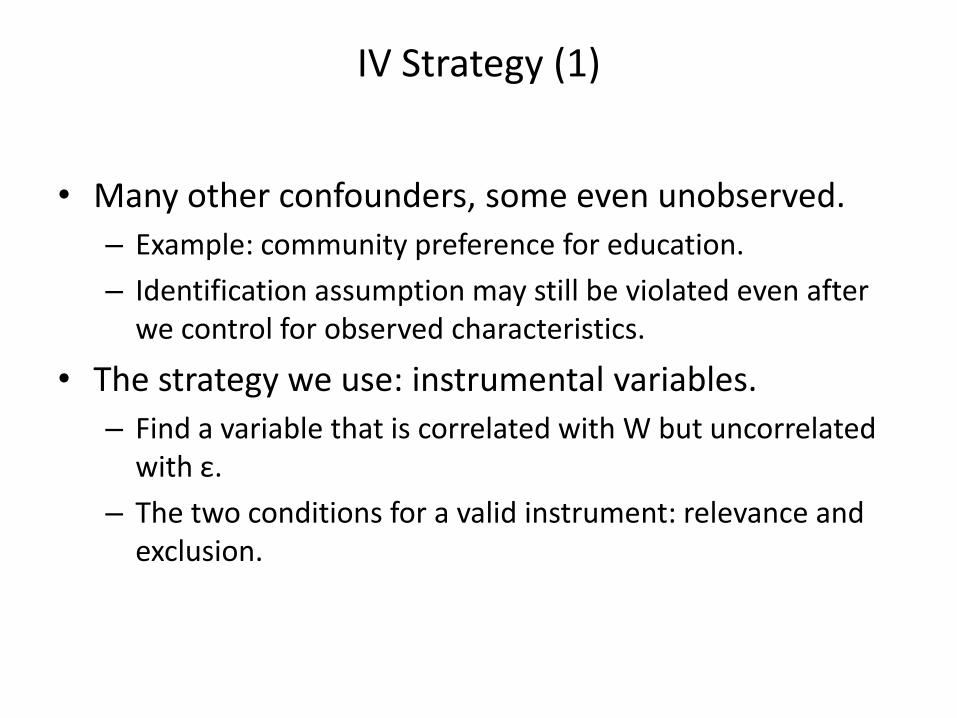
IV Strategy (1)

• Many other confounders, some even unobserved.

– Example: community preference for education.

– Identification assumption may still be violated even after we control for observed characteristics.

• The strategy we use: instrumental variables.

– Find a variable that is correlated with W but uncorrelated with ε.

– The two conditions for a valid instrument: relevance and exclusion.

IV Strategy (2)

• Instruments used in the literature: – local economy, adult labor market conditions, or prices; school

quality and availability; household assets; compulsory school starting age.

• Our instrument– Basu (00): an increase in legislated minimum wage may increase

child labor under certain conditions, by affecting demand or supply of child workers.• Feature 1: child workers are not covered by the minimum wage

legislation.

• Feature 2: child labor can (perfectly) substitute adult labor, with a certain coefficient.

– Legislated minimum wage levels at the year and in the province a child worker began working.

– For non-child workers, we impute the year that they would have begun working based on birth year.

IV: Relevance

Dependent variable: Child labor status (=1) (1) (2) (3)

coef se coef se coef se

Provincial monthly legislated minimum wage (hundred

thousand Rupiah)

0.158** 0.051 0.307** 0.077 0.432** 0.058

Male (=1) 0.001 0.012 -0.001 0.013

Age in 2007 0.044** 0.005 0.049** 0.004

Father's schooling (years) -0.008** 0.002 -0.007** 0.002

District GDP per capita in 1996 (millions, 1993 Rupiah) -0.015** 0.006 -0.014* 0.006

Proportion of villages in the district with a market building 0.332 0.175

Proportion of villages in the district with year-round roads -0.039 0.139

Proportion of villages in the district with a formal financial

institution

-0.124 0.072

Proportion of villages in the district with a public health

center

-0.242 0.133

Number of primary and secondary schools in the district

(thousand)

-0.054** 0.019

Constant -0.109 0.067 -1.068** 0.159 -1.258** 0.186

Number of observations 2,675 2,675 2,675

R-squared 0.016 0.101 0.126

Notes ** p<0.01, * p<0.05; estimated using OLS; standard errors are clustered at the province level; the provincial minimum

wage depends on the year that a child worker began working or a non-child worker is predicted to have begun working

IV: Exclusion (1)

• Minimum wage legislation in Indonesia

– Based on a bundle of consumption items, around 2,600 –3,000 kcal/day (Suryahadi et al, 03).

– Up to 2000, each province has a single minimum wage level, determined through tripartite discussion.

– The minimum wage level in a province is a function of province-specific prices and negotiation results.

• Therefore, unlikely to have a direct causal relationship with the dependent variables.

IV: Exclusion (2)

• Correlation between minimum wage and ε:

– Fundamentally untestable, but we can still measure the correlation between minimum wage with several variables likely to be in the residual.

– Infrastructure – to measure unobserved economic-related factors.

– Availability of education and health facilities – proxy for unobserved community preferences.

– Labor market conditions and household expenditure data.

IV: Exclusion (3)

District Population Proportion of

villages in the

district with a

market building

Proportion of

villages in the

district with

year-round roads

coef s.e. coef s.e. coef s.e.

Provincial monthly legislated minimum wage

(hundred thousand Rupiah)

756,763.4 479,166.1 -0.008 0.108 -0.034 0.051

Constant -224,761.6 595,793.5 0.242* 0.136 1.001** 0.071

Number of observations 177 177 177

R-squared 0.097 0.000 0.009

Regression level District District District

IV: Exclusion (4)

Proportion of

villages in the

district with a

formal financial

institution

Proportion of

villages in the

district with a

public health

center

Number of

primary and

secondary

schools in the

district

(thousand)




0.097 0.189 0.185 0.154 0.602 0.309

Constant 0.123 0.248 -0.076 0.194 0.005 0.382

Number of observations 177 177 177

R-squared 0.010 0.087 0.082

Regression level District District District

IV: Exclusion (5)

District Adult

Unemployment

Rate in 2000

Father is

employed in 2000

(=1)

Log of per capita

monthly household

expenditure in

2000




0.032 0.017 0.007 0.062 0.044 0.154

Constant 0.018 0.021 0.554** 0.069 12.178** 0.204

Number of observations 177 2,614 2,641

R-squared 0.034 0.000 0.000

Regression level District Household Household

note: ** p<0.01, * p<0.05; standard errors are clustered at the province level; estimated using OLS.

ESTIMATION RESULTS

How big is big?

• The dependent variable is in standard deviations.

• In education literature, 0.3 SD is considered a large effect.

• In Indonesia, one year of schooling produces 0.13 SD of math ability.

• In IFLS 2000, the difference between the median and the 75th

percentile is 1 SD.

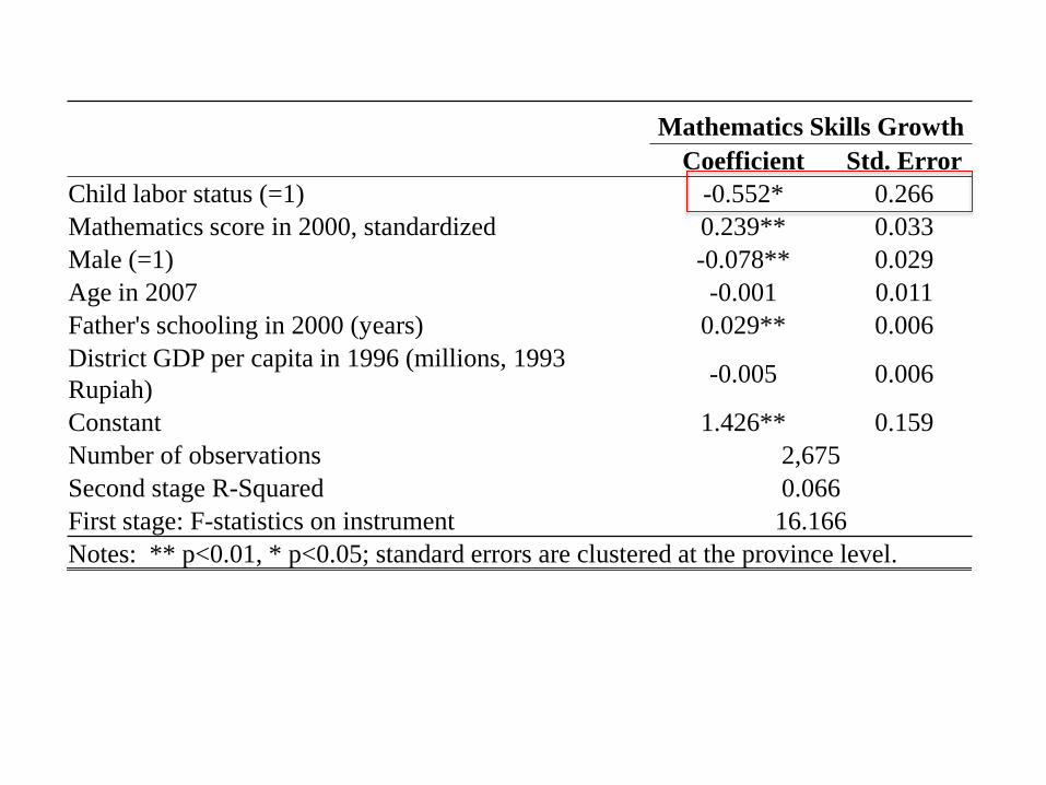
Mathematics Skills Growth

Coefficient Std. Error

Child labor status (=1) -0.552* 0.266

Mathematics score in 2000, standardized 0.239** 0.033

Male (=1) -0.078** 0.029

Age in 2007 -0.001 0.011

Father's schooling in 2000 (years) 0.029** 0.006

District GDP per capita in 1996 (millions, 1993

Rupiah)-0.005 0.006

Constant 1.426** 0.159

Number of observations 2,675

Second stage R-Squared 0.066

First stage: F-statistics on instrument 16.166

Notes: ** p<0.01, * p<0.05; standard errors are clustered at the province level.

Cognitive Skills Growth


Child labor status (=1) -0.476 0.370

Cognitive score in 2000, standardized 0.222** 0.033

Male (=1) 0.070* 0.031

Age in 2007 0.010 0.016

Father's schooling in 2000 (years) 0.024** 0.007


Rupiah)0.001 0.006

Constant 2.207** 0.255





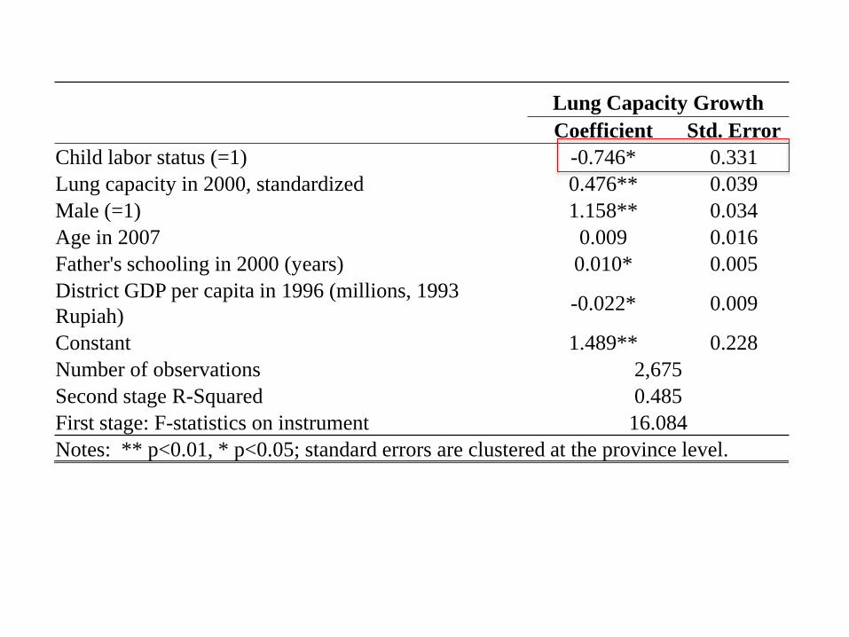
Lung Capacity Growth


Child labor status (=1) -0.746* 0.331

Lung capacity in 2000, standardized 0.476** 0.039

Male (=1) 1.158** 0.034

Age in 2007 0.009 0.016

Father's schooling in 2000 (years) 0.010* 0.005


Rupiah)-0.022* 0.009

Constant 1.489** 0.228





Gender heterogeneity

• No significant gender difference in child market work participation rate, type/place of work, or working hours.

• However, there is significant difference in sectoralcomposition of the occupation.

– Higher share of boys working in agriculture; higher share of girls working as housemaids.

• Even for children in the same sector, males and females may do different tasks (Edmonds, 08).

Mathematics Skills

Growth Cognitive Skills

Growth

Lung Capacity

Growth

CoefStd.

ErrorCoef

Std.

ErrorCoef

Std.

Error

MALE

Child Labor Status (=1) -0.302 0.293 -0.471* 0.238 -0.791* 0.344

N 1,365 1,365 1,365

R-Squared 0.099 0.032 0.110

First-stage F Statistics 13.406 13.700 12.932

FEMALE

Child Labor Status (=1) -0.910* 0.407 -0.557 0.716 -0.667 0.447

N 1,310 1,310 1,310

R-Squared -0.018 0.117 -0.014


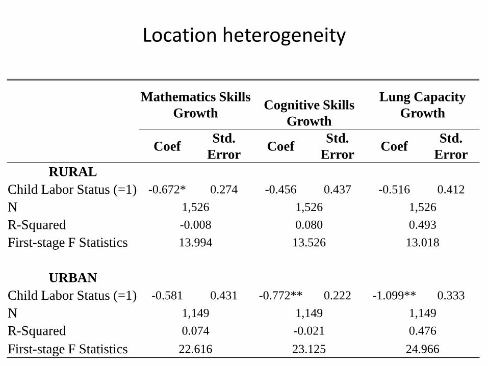
Location heterogeneity

Mathematics Skills


Growth

Lung Capacity

Growth

CoefStd.

ErrorCoef

Std.

ErrorCoef

Std.

Error

RURAL

Child Labor Status (=1) -0.672* 0.274 -0.456 0.437 -0.516 0.412

N 1,526 1,526 1,526

R-Squared -0.008 0.080 0.493


URBAN

Child Labor Status (=1) -0.581 0.431 -0.772** 0.222 -1.099** 0.333

N 1,149 1,149 1,149

R-Squared 0.074 -0.021 0.476


Type of work heterogeneity

• Type of work in 2000:

– 87% work for the family business, usually unpaid.

– 20% work for wage outside family.

– 6% work both types

• Although unpaid, children working in the family business may face better conditions.

• This aspect of child labor is much less explored.

• Potential issue

– Choice of type of work may be endogenous.

– We do not model this choice.

Mathematics Skills


Growth

Lung Capacity

Growth

CoefStd.

ErrorCoef

Std.

ErrorCoef

Std.

Error

FAMILY

BUSINESS

Child Labor Status (=1) -0.785 0.427 -0.734 0.537 -1.104* 0.549

N 2,611 2,611 2,611

R-Squared 0.032 0.042 0.430


FOR WAGE OUTSIDE

Child Labor Status (=1) -1.253 0.691 -0.767 0.780 -1.401** 0.528

N 2,403 2,403 2,403

R-Squared 0.077 0.108 0.499


Conclusion (1)

• We find child market work to have a significant negative and large effect on growth of human capital over a seven-year period.– Similarly large for math skills, cognitive skills, and health.

• Gender heterogeneity– Male and female child workers suffer about the same in terms of

health and cognitive skills growth; statistically significant only for males.

– Female child workers suffer much worse in terms of mathematics skills growth.

• Type of work heterogeneity– Results only suggestive due to data and estimation difficulties.

– Child workers working for pay outside the household seem to bear worse effects of market work.

Conclusion (2)

• Take home messages:– Focusing on output measures of human capital unearth large negative

effects of child labor.

– These effects are observed even when 90% of the child workers are working for the family business, and 20% work outside the family.

– Even the “acceptable” child labor have severe detrimental effects on human capital.

the consequences of child labor on the growth of human

Documents