The cone conditionand nonsmoothness in

linear generalized Nash games

Oliver Stein∗ Nathan Sudermann-Merx#

April 13, 2015

Abstract

We consider linear generalized Nash games and introduce the so-called cone condition which characterizes the smoothness of the Nikai-do-Isoda function under weak assumptions. The latter mapping arisesfrom a reformulation of the generalized Nash equilibrium problem asa possibly nonsmooth optimization problem.

Other regularity conditions like LICQ or SMFC(Q) are only suffi-cient for smoothness, but have the advantage that they can be veri-fied more easily than the cone condition. Therefore, we present specialcases where these conditions are not only sufficient, but also necessaryfor smoothness of the Nikaido-Isoda function.

Our main tool in the analysis is a global extension of the Nikaido-Isoda function that allows us to avoid technical issues that may appearat the boundary of the domain of the Nikaido-Isoda function.

Keywords: generalized Nash equilibrium problem; Nikaido-Isoda function;piecewise-linear function; genericity; parametric optimization; constraint qual-ification

AMS subject classifications: 91A06; 91A10; 90C31

Preliminary citation: Optimization Online, Preprint ID 2015-03-4847,2015.

∗Institute of Operations Research, Karlsruhe Institute of Technology (KIT), Germany,stein@kit.edu

#Institute of Operations Research, Karlsruhe Institute of Technology (KIT), Germany,sudermann@kit.edu

1 Introduction

In a generalized Nash equilibrium problem (GNEP) each player ν ∈ {1, . . . , N},N ∈ N, controls a decision vector xν ∈ R

nν , nν ∈ N, and wishes to solve hisparametric optimization problem

Qν(x−ν) : min

xν∈Rnν

θν(xν , x−ν) s.t. xν ∈ Xν(x

−ν)

given the other players’ decisions x−ν ∈ Rn−nν , with n := n1 + . . . + nN .

For fixed x−ν ∈ Rn−nν , we call θν(·, x

−ν) : Rnν → R the cost function andXν(x

−ν) ⊆ Rnν the strategy set of player ν. A GNEP consists of finding

some x := (xν , x−ν) ∈ Rn, such that xν is an optimal point of Qν(x

−ν) foreach ν = 1, . . . , N .

In contrast to the classical Nash equilibrium problem (NEP), player ν’s strat-egy set Xν(x

−ν) may depend on the decisions of the remaining players x−ν ,whereas the strategy sets Xν are fixed in NEPs. A typical situation thatimplies the x−ν-dependence of the strategy sets is the appearance of sharedconstraints.

NEPs were introduced in [16] and GNEPs go back to [1] and [5]. Overviewsof applications a well as theoretical and numerical results on GNEPs aregiven in [9] and [10].

In the present paper we shall assume linearity of the cost functions and theconstraints of all players in the whole vector x, that is for each ν ∈ {1, . . . , N},there exist an integer mν ∈ N, matrices Aν ∈ R

mν×nν , Bν ∈ Rmν×(n−nν) and

vectors aν ∈ Rnν , cν ∈ R

mν , such that player ν’s optimization problem canbe expressed as

Qν(x−ν) : min

xν∈Rnν

〈aν , xν〉 s.t. Aνxν + Bνx−ν ≤ cν .

Hence, throughout this paper we shall have

θν(xν , x−ν) = 〈aν , xν〉

andXν(x

−ν) = {xν ∈ Rnν | Aνxν ≤ cν − Bνx−ν}

for all ν ∈ {1, . . . , N}. Note that it would add no generality to augmentplayer ν’s cost function θν by a term 〈bν , x−ν〉 or even by a nonlinear functionf(x−ν), because this would only affect its optimal value, but not its optimalpoint.

2

For each ν ∈ {1, . . . , N} we denote by

domXν := {x−ν ∈ Rn−nν | Xν(x

−ν) 6= ∅}

the (effective) domain of the set-valued mapping Xν . Throughout this articlewe will use the subsequent assumption which would follow, for example, fromthe boundedness of all strategy sets.

Assumption 1.1 For any ν ∈ {1, . . . , N} and x−ν ∈ domXν the problemQν(x

−ν) is solvable.

Since in our setting all defining functions are linear, we call this special casea linear generalized Nash equilibrium problem (LGNEP). To the best of ourknowledge, up to now there do not exist systematic treatments of LGNEPsin the literature. The closest setting is the one of affine generalized Nashequilibrium problems (AGNEPs), where GNEPs with linear constraints andquadratic cost functions are considered which are convex in the player vari-ables. This setting was introduced explicitly in [20] and also investigatedin [6, 7]. Various examples of GNEPs where players share affine constraintsare summarized in [20]. Furthermore, the very common case of players hav-ing finite strategy sets and minimizing their expected losses, allowing mixedstrategies, yields special LGNEPs (cf. [17]).

Particularly, LGNEPs always arise in a natural way if several players solve lin-ear problems while sharing at least one constraint. To illustrate this thoughtlet us think of the transportation problem, a standard application of linearprogramming. In the classical transportation problem there is one forwarderwho minimizes his costs of distributing a good from manufacturers to con-sumers. In the next example we will model the transportation problem forseveral forwarders and arrive at a LGNEP.

Example 1.2 Consider n manufacturers having a production capacity of Si,i ∈ {1, . . . , n}, for one good that is supplied by p competing forwarding agen-cies to m consumers. Each consumer j ∈ {1, . . . ,m} needs at least Dj unitsof this good. The transportation cost of one unit from manufacturer i toconsumer j by forwarder k ∈ {1, . . . , p} is denoted by akij. The transportedunits from manufacturer i to consumer j by the forwarder k are denoted byxkij. Now each forwarder wants to minimize his transportation costs, given

the decisions of the remaining forwarders:

Qk(x−k) : min

xk∈Rm×n

n∑

i=1

m∑

j=1

akijxkij s.t.

∑m

j=1

∑p

ℓ=1 xℓij ≤ Si, i = 1, . . . , n

∑n

i=1

∑p

ℓ=1 xℓij ≥ Dj, j = 1, . . . ,m.

3

The search for a combination xkij, such that the matrix (xk

ij) solves player k’soptimization problem for all k ∈ {1, . . . , p} yields a linear generalized Nashequilibrium problem where all players share the same constraints.

We emphasize that GNEPs are often studied under more general structuralassumptions, in particular so-called joint or player convexity, respectively(cf., e.g., [9]). Under player convexity, smoothness properties of the associ-ated Nikaido-Isoda function are studied in [11], but technical issues arise atboundary points of the domain of this function. There, this also leads to therestriction of the presented numerical approach to a feasible point methodfor the solution of the corresponding optimization problem. In contrast, un-der the assumptions of the present paper we will be able to define a globalextension of the Nikaido-Isoda function, so that these issues do not occur.

This article is structured as follows. In Section 2 we restate some well-knownfacts about the Nikaido-Isoda function and construct a global extension ofthe Nikaido-Isoda function in order to overcome the common difficulty thatthe domain of the Nikaido-Isoda function may not cover the whole space.The construction of the global extension heavily exploits the duality theoryof linear programming and is therefore not available in the nonlinear settingwithout further assumptions.

In Section 3 we examine the position of nondifferentiability points of theNikaido-Isoda function by providing necessary and sufficient conditions fortheir location in terms of regularity conditions. Particularly, we introducethe so-called cone condition that captures the nonsmoothness of the Nikaido-Isoda function very sharply and even characterizes its location under weakassumptions. Other regularity conditions like LICQ or SMFC(Q) are onlysufficient for smoothness, but have the advantage that they can be verifiedmore easily than the cone condition. Therefore, we present special caseswhere these conditions are not only sufficient, but also necessary for smooth-ness of the Nikaido-Isoda function.

In Section 4 we show that most of our assumptions hold generically, that is,they are valid on an open and dense subset of the defining data of LGNEP.The article closes with some final remarks in Section 5, where we also sketchpossible applications of our results to optimality conditions and numericalmethods.

4

2 Global extension of the Nikaido-Isoda func-

tion

For x ∈ Rn and ν ∈ {1, . . . , N} we define player ν’s optimal value function

ϕν(x−ν) :=

{minxν∈Xν(x−ν) 〈a

ν , xν〉, if x−ν ∈ domXν

+∞, else,

and the so-called Nikaido-Isoda function

V (x) :=N∑

ν=1

〈aν , xν〉 − ϕν(x−ν),

which, under Assumption 1.1, is real-valued on the set

M :=⋂

ν=1,...,N

(Rnν × domXν),

whereas we have V (x) = −∞ for x 6∈ M . Particularly, in general the domainof V does not cover the whole space, which causes numerical and theoreticaldifficulties (see, e.g. [11] and [22], resp.).

According to [8], the function V is nonnegative on the unfolded commonstrategy set

W := {x ∈ Rn| Aνxν + B−νx−ν ≤ cν , ν = 1, . . . , N}

= {x ∈ Rn| xν ∈ Xν(x

−ν), ν = 1, . . . , N} ⊆ M.

These properties yield the following result, which also holds under consider-ably weaker assumptions (cf., e.g., [12]).

Proposition 2.1 The generalized Nash equilibria of LGNEP are the globalminimal points of the (possibly non-smooth) optimization problem

min V (x) s.t. x ∈ W

with optimal value zero.

We will use the following example throughout this article to illustrate ourresults. Note that the example is stable in the sense that small perturbationsin the defining data do not imply qualitative changes in our results.

5

Example 2.2 Let us consider a LGNEP with two players, each having aone-dimensional strategy set, that is, n1 = n2 = 1 and therefore N = n =2. To simplify the notation, we denote the decision variable of player oneby x1 and of the second player by x2, respectively. The players share threeconstraints given by

−1

2

1−1

x1 +

1−1−1

x2 ≤

111

.

Furthermore, the objective functions are θ1(x1) = −x1 and θ2(x2) = x2. Thenwe obtain the optimal value functions

ϕ1(x2) =

{−x2 − 1 , x2 ∈ domX1 = [−1, 3]

∞ , else

and

ϕ2(x1) =

{|x1| − 1 , x1 ∈ domX2 = [−4

3, 4]

∞ , else,

so that the Nikaido-Isoda function is given by

V (x) =

{2− x1 − |x1|+ 2x2 , x ∈ M = [−4

3, 4]× [−1, 3]

−∞ , else.

The generalized Nash equilibria form the line segment [(0,−1), (4, 3)].

The sets W and M as well as the graph of V on W are illustrated in Figures 1and 2, respectively.

4

3

−1

x1

W

x2

−43

M

Figure 1: Illustration of the sets W and M in Example 2.2

As Example 2.2 illustrates, the minimization of V over W may be a non-smooth optimization problem, so that below we shall study smoothness prop-erties of V . As V is only real-valued on the set M , first we will construct

6

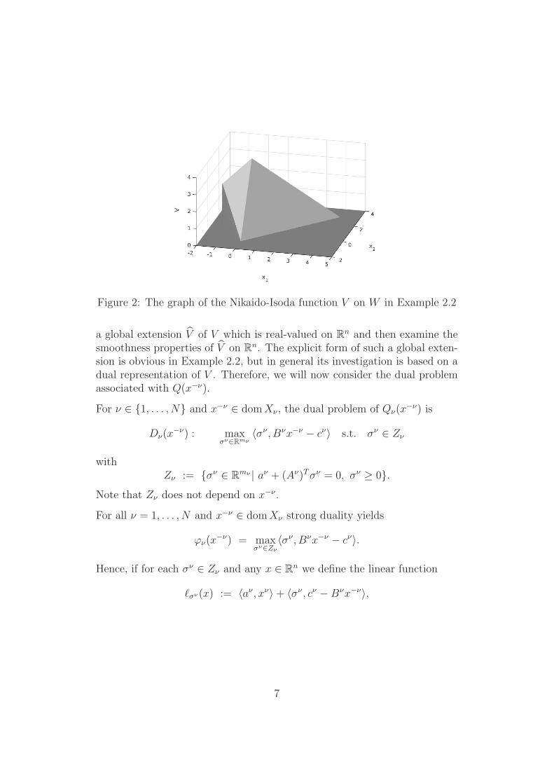
Figure 2: The graph of the Nikaido-Isoda function V on W in Example 2.2

a global extension V of V which is real-valued on Rn and then examine the

smoothness properties of V on Rn. The explicit form of such a global exten-

sion is obvious in Example 2.2, but in general its investigation is based on adual representation of V . Therefore, we will now consider the dual problemassociated with Q(x−ν).

For ν ∈ {1, . . . , N} and x−ν ∈ domXν , the dual problem of Qν(x−ν) is

Dν(x−ν) : max

σν∈Rmν

〈σν , Bνx−ν − cν〉 s.t. σν ∈ Zν

withZν := {σν ∈ R

mν | aν + (Aν)Tσν = 0, σν ≥ 0}.

Note that Zν does not depend on x−ν .

For all ν = 1, . . . , N and x−ν ∈ domXν strong duality yields

ϕν(x−ν) = max

σν∈Zν

〈σν , Bνx−ν − cν〉.

Hence, if for each σν ∈ Zν and any x ∈ Rn we define the linear function

ℓσν (x) := 〈aν , xν〉+ 〈σν , cν −Bνx−ν〉,

7

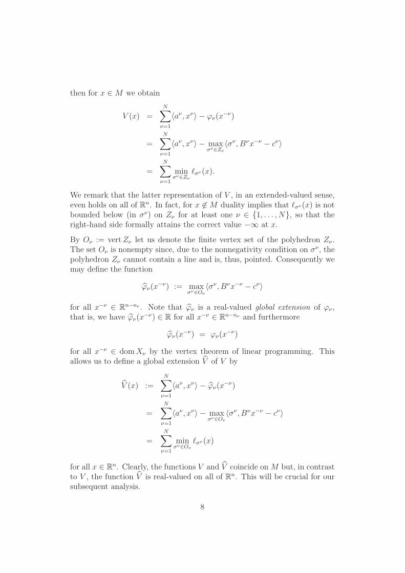
then for x ∈ M we obtain

V (x) =N∑

ν=1

〈aν , xν〉 − ϕν(x−ν)

=N∑

ν=1

〈aν , xν〉 − maxσν∈Zν

〈σν , Bνx−ν − cν〉

=N∑

ν=1

minσν∈Zν

ℓσν (x).

We remark that the latter representation of V , in an extended-valued sense,even holds on all of Rn. In fact, for x 6∈ M duality implies that ℓσν (x) is notbounded below (in σν) on Zν for at least one ν ∈ {1, . . . , N}, so that theright-hand side formally attains the correct value −∞ at x.

By Oν := vertZν let us denote the finite vertex set of the polyhedron Zν .The set Oν is nonempty since, due to the nonnegativity condition on σν , thepolyhedron Zν cannot contain a line and is, thus, pointed. Consequently wemay define the function

ϕν(x−ν) := max

σν∈Oν

〈σν , Bνx−ν − cν〉

for all x−ν ∈ Rn−nν . Note that ϕν is a real-valued global extension of ϕν ,

that is, we have ϕν(x−ν) ∈ R for all x−ν ∈ R

n−nν and furthermore

ϕν(x−ν) = ϕν(x

−ν)

for all x−ν ∈ domXν by the vertex theorem of linear programming. Thisallows us to define a global extension V of V by

V (x) :=N∑

ν=1

〈aν , xν〉 − ϕν(x−ν)

=N∑

ν=1

〈aν , xν〉 − maxσν∈Oν

〈σν , Bνx−ν − cν〉

=N∑

ν=1

minσν∈Oν

ℓσν (x)

for all x ∈ Rn. Clearly, the functions V and V coincide on M but, in contrast

to V , the function V is real-valued on all of Rn. This will be crucial for oursubsequent analysis.

8

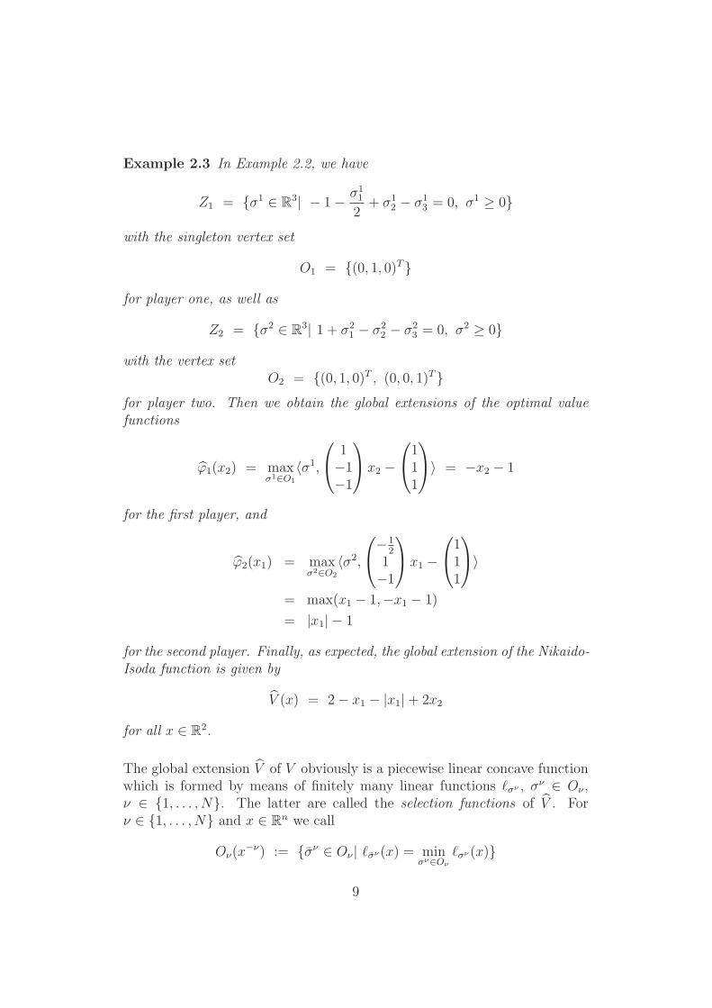
Example 2.3 In Example 2.2, we have

Z1 = {σ1 ∈ R3| − 1−

σ11

2+ σ1

2 − σ13 = 0, σ1 ≥ 0}

with the singleton vertex set

O1 = {(0, 1, 0)T}

for player one, as well as

Z2 = {σ2 ∈ R3| 1 + σ2

1 − σ22 − σ2

3 = 0, σ2 ≥ 0}

with the vertex setO2 = {(0, 1, 0)T , (0, 0, 1)T}

for player two. Then we obtain the global extensions of the optimal valuefunctions

ϕ1(x2) = maxσ1∈O1

〈σ1,

1−1−1

x2 −

111

〉 = −x2 − 1

for the first player, and

ϕ2(x1) = maxσ2∈O2

〈σ2,

−1

2

1−1

x1 −

111

〉

= max(x1 − 1,−x1 − 1)

= |x1| − 1

for the second player. Finally, as expected, the global extension of the Nikaido-Isoda function is given by

V (x) = 2− x1 − |x1|+ 2x2

for all x ∈ R2.

The global extension V of V obviously is a piecewise linear concave functionwhich is formed by means of finitely many linear functions ℓσν , σν ∈ Oν ,ν ∈ {1, . . . , N}. The latter are called the selection functions of V . Forν ∈ {1, . . . , N} and x ∈ R

n we call

Oν(x−ν) := {σν ∈ Oν | ℓσν (x) = min

σν∈Oν

ℓσν (x)}

9

the index set of active selection functions of player ν at x−ν . Note that forν ∈ {1, . . . , N} the set Oν(x

−ν) is nonempty, and that it does not depend onxν since the condition ℓσν (x) = minσν∈Oν

ℓσν (x) is equivalent to

〈σν , Bνx−ν − cν〉 = maxσν∈Oν

〈σν , Bνx−ν − cν〉. (1)

Due to (1), we may also write

Oν(x−ν) = {σν ∈ Oν | 〈σ

ν , Bνx−ν − cν〉 = ϕν(x−ν)}. (2)

For a given point x ∈ Rn the sets Oν(x

−ν), ν ∈ {1, . . . , N}, already determine

the local behavior of V around x:

Proposition 2.4 For each x ∈ Rn there exists a neighborhood U of x with

V (x) =N∑

ν=1

minσν∈Oν(x−ν)

ℓσν (x)

for all x ∈ U .

Proof. Let x ∈ Rn. Then for all ν ∈ {1, . . . , N} we have Oν(x

−ν) ⊆ Zν andtherefore

V (x) =N∑

ν=1

minσν∈Zν

ℓσν (x) ≤N∑

ν=1

minσν∈Oν(x−ν)

ℓσν (x)

for all x ∈ Rn.

For the reverse inequality, we show for each ν ∈ {1, . . . , N} the existenceof a neighborhood Uν of x with Oν(x

−ν) ⊆ Oν(x−ν) for all x ∈ Uν . In

the case Oν(x−ν) = Oν this is trivially satisfied. Otherwise, choose any

σν ∈ Oν \Oν(x−ν). Then, in view of (1), we have

〈σν , Bν x−ν − cν〉 < maxσν∈Oν(x−ν)

〈σν , Bν x−ν − cν〉.

Continuity and the finiteness of the set Oν(x−ν) ensure the existence of a

neighborhood Uσν of x with

〈σν , Bνx−ν − cν〉 < maxσν∈Oν(x−ν)

〈σν , Bνx−ν − cν〉.

for all x ∈ Uσν . For all x from the finite intersection

Uν :=⋂

σν∈Oν\Oν(x−ν)

Uσν

10

we thus have

〈σν , Bνx−ν − cν〉 < maxσν∈Oν(x−ν)

〈σν , Bνx−ν − cν〉

which means σν ∈ Oν \Oν(x−ν). Hence we arrive at Oν(x

−ν) ⊆ Oν(x−ν) for

all x ∈ Uν , and the set U :=⋂

ν=1,...,N Uν is the asserted neighborhood of x.•

Player ν’s index set of active selection functions Oν(x−ν) at x−ν is of course

intimately related to dual information. In fact, for ν ∈ {1, . . . , N} andx−ν ∈ domXν let

Sν(x−ν) := {xν ∈ Xν(x

−ν)| 〈aν , xν〉 = ϕν(x−ν)}

denote the (nonempty) set of optimal points of Qν(x−ν), and for any yν ∈

Sν(x−ν) let

KKTν(x−ν) := {σν ∈ Zν | 〈σ

ν , Aνyν +Bνx−ν − cν〉 = 0}

denote the corresponding set of Karush-Kuhn-Tucker (KKT) multipliers.Note that the latter set may be rewritten as

KKTν(x−ν) = {σν ∈ Zν | 〈σ

ν , Bνx−ν − cν〉 = ϕν(x−ν)}

so that it does not depend on the actual choice of yν ∈ Sν(x−ν).

Proposition 2.5 For all ν ∈ {1, . . . , N} and x−ν ∈ domXν the set Oν(x−ν)

coincides with the vertex set of KKTν(x−ν).

Proof. The dually optimal set KKTν(x−ν) is a face of Zν . Thus, the vertex

set of KKTν(x−ν) coincides with the set

KKTν(x−ν) ∩ vert(Zν) = {σν ∈ Oν | 〈σ

ν , Bνx−ν − cν〉 = ϕν(x−ν)}

= Oν(x−ν),

where the last equality holds due to (2) and the vertex theorem of linearprogramming. •

For any ν ∈ {1, . . . , N} and x−ν ∈ domXν , Proposition 2.5 states thatOν(x

−ν) coincides with the vertex set of KKTν(x−ν) and, thus, establishes a

link between the ’primal’ index set of active selection functions Oν(x−ν) and

the ’dual’ set of vertex KKT multipliers vertKKTν(x−ν). More importantly,

11

it shows that the set-valued mapping Oν : Rn−nν ⇒ Rmν is a global extension

of the set-valued mapping vertKKTν : domXν ⇒ Rnν .

According to Propositions 2.4 and 2.5, the local behavior of V on M andoutside of M is governed by vertex KKT multipliers and their global exten-sions by active index sets of selection functions, respectively. We will heavilyexploit this connection in Section 3.

3 Smoothness of the Nikaido-Isoda function

Recall that the Nikaido-Isoda function V is not real-valued outside of the setM . For a smoothness analysis of V on W ⊆ M , this may cause technicalissues at boundary points of W in cases where these also are boundary pointsofM (cf. Fig. 1). Fortunately, we may analyze its global extension V instead.

Since V is piecewise linear on Rn, in the following the notion of ’local linearity’

is chosen to describe its smoothness properties at a given reference point.

Definition 3.1 We call the extended Nikaido-Isoda function V locally lin-ear in x ∈ R

n if there exist an affine linear function A : Rn → R and aneighborhood U of x with V (x) = A(x) for all x ∈ U .

We will use the terms ’smooth’ and ’locally linear’ synonymously in thisarticle. Analogously, we shall denote V as ’nonsmooth’ in a reference point,if it is not locally linear there.

In the following sections, based on an examination of the directional deriva-tives of V , we will explore the connection between smoothness of V and someregularity conditions, particularly, the so-called cone condition.

3.1 Directional derivatives

Let x ∈ Rn and d ∈ R

n. The (one-sided) directional derivative of V in xalong d is defined by

V ′(x, d) := limtց0

V (x+ td)− V (x)

t.

The following result immediately follows from the additivity of the directionalderivative and the formula for directional derivatives of max-functions from,e.g., [4].

12

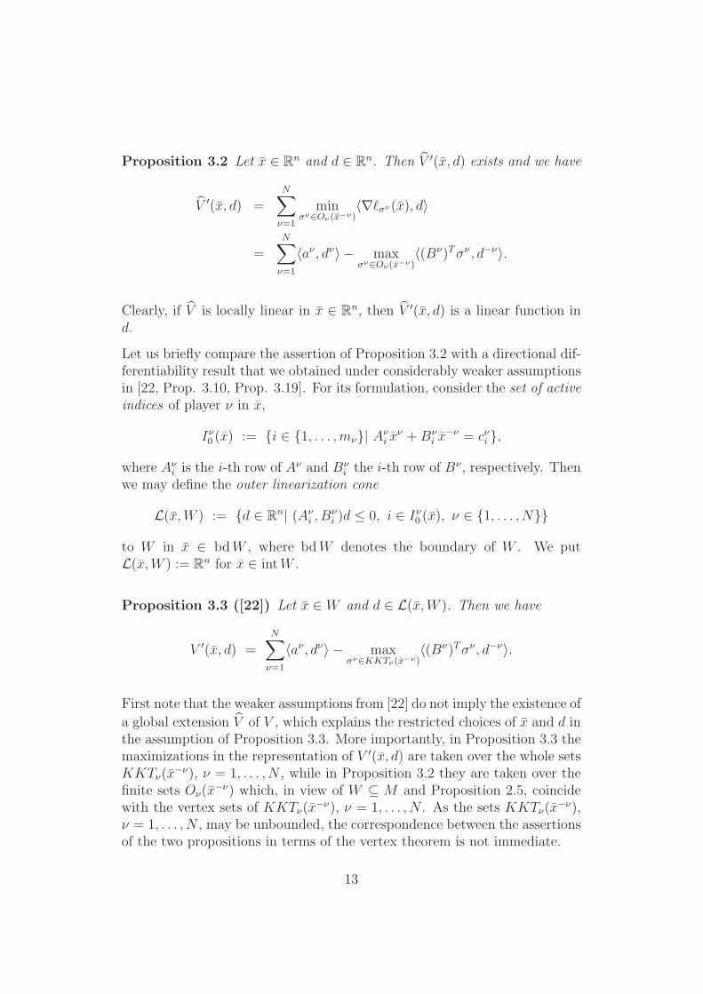
Proposition 3.2 Let x ∈ Rn and d ∈ R

n. Then V ′(x, d) exists and we have

V ′(x, d) =N∑

ν=1

minσν∈Oν(x−ν)

〈∇ℓσν (x), d〉

=N∑

ν=1

〈aν , dν〉 − maxσν∈Oν(x−ν)

〈(Bν)Tσν , d−ν〉.

Clearly, if V is locally linear in x ∈ Rn, then V ′(x, d) is a linear function in

d.

Let us briefly compare the assertion of Proposition 3.2 with a directional dif-ferentiability result that we obtained under considerably weaker assumptionsin [22, Prop. 3.10, Prop. 3.19]. For its formulation, consider the set of activeindices of player ν in x,

Iν0 (x) := {i ∈ {1, . . . ,mν}| Aνi x

ν + Bνi x

−ν = cνi },

where Aνi is the i-th row of Aν and Bν

i the i-th row of Bν , respectively. Thenwe may define the outer linearization cone

L(x,W ) := {d ∈ Rn| (Aν

i , Bνi )d ≤ 0, i ∈ Iν0 (x), ν ∈ {1, . . . , N}}

to W in x ∈ bdW , where bdW denotes the boundary of W . We putL(x,W ) := R

n for x ∈ intW .

Proposition 3.3 ([22]) Let x ∈ W and d ∈ L(x,W ). Then we have

V ′(x, d) =N∑

ν=1

〈aν , dν〉 − maxσν∈KKTν(x−ν)

〈(Bν)Tσν , d−ν〉.

First note that the weaker assumptions from [22] do not imply the existence of

a global extension V of V , which explains the restricted choices of x and d inthe assumption of Proposition 3.3. More importantly, in Proposition 3.3 themaximizations in the representation of V ′(x, d) are taken over the whole setsKKTν(x

−ν), ν = 1, . . . , N , while in Proposition 3.2 they are taken over thefinite sets Oν(x

−ν) which, in view of W ⊆ M and Proposition 2.5, coincidewith the vertex sets of KKTν(x

−ν), ν = 1, . . . , N . As the sets KKTν(x−ν),

ν = 1, . . . , N , may be unbounded, the correspondence between the assertionsof the two propositions in terms of the vertex theorem is not immediate.

13

3.2 The cone condition

From Proposition 2.4 we see that locally around any point x ∈ Rn the func-

tion V is constituted as the sum of pointwise minima of linear functions,indexed by the set of active selection functions Oν(x

−ν). If Oν(x−ν) is a

singleton for all ν ∈ {1, . . . , N} then, obviously, V is smooth at x.

Definition 3.4 For ν ∈ {1, . . . , N} and x−ν ∈ Rn−nν we say that the player

cone condition (PCC) is valid in x−ν if Oν(x−ν) contains at most one ele-

ment. We say that the collective cone condition (CCC) holds in x ∈ Rn if

PCC holds in x−ν for all ν ∈ {1, . . . , N}.

We emphasize that, as Oν(x−ν) is not void, CCC at x ∈ R

n actually impliesthat Oν(x

−ν) is a singleton for all ν ∈ {1, . . . , N}.

Remark 3.5 Since, in view of Proposition 2.5, for all ν ∈ {1, . . . , N} andx−ν ∈ domXν the set Oν(x

−ν) coincides with the vertex set of the polyhedronKKTν(x

−ν), the player cone condition states for these x−ν that KKTν(x−ν)

possesses at most one vertex or, equivalently, that it is a (translated) convexcone. This explains the terminology in Definition 3.4.

As discussed above, the following result immediately follows from Proposi-tion 2.4.

Proposition 3.6 If CCC holds in x ∈ Rn, then V is smooth in x.

The next example illustrates the interplay between CCC and smoothness ofV .

Example 3.7 In Example 2.2, by direct inspection it is immediate that thenon-differentiability points of V form the set

ND := {x ∈ R2| x1 = 0}.

Since O1 and, thus, the sets O1(x2) are singletons for all x2 ∈ R, PCC holdsfor player one in each x2 ∈ R. Furthermore, we have |O2(x1)| > 1 if andonly if x1 = 0, so that PCC holds for player two in x1 ∈ R if and only ifx1 6= 0. Consequently, CCC in x ∈ R

2 is violated exactly on the set ND and,in this example, CCC even characterizes the smoothness of V .

14

The latter example indicates that the collective cone condition might be asuitable tool to examine the nonsmoothness structure of V . Actually, as wewill see below, the collective cone condition characterizes the smoothness ofV under mild assumptions. Before we show this, we need some auxiliaryconcepts and results.

For ν ∈ {1, . . . , N} and σν ∈ Oν we define the index set of positive multipliersof player ν at σν by

I+(σν) := {i ∈ {1, . . . ,mν}| σ

νi > 0}.

In the next lemma we obtain an upper bound to the number of non-vanishingmultipliers.

Lemma 3.8 Let ν ∈ {1, . . . , N} and σν ∈ Oν. Then we have |I+(σν)| ≤ nν.

Proof. Let σ be a vertex of

Zν = {σν ∈ Rmν | aν + (Aν)Tσν = 0, σν ≥ 0}.

Then, by definition, the rank of the gradients that belong to active constraintsequals mν . More formally, the rank of the mν × (nν + |I+(σ

ν)c|)-matrix(Aν |eI+(σν)c

)

is mν , where eI+(σν)c is a matrix whose columns are the mν-dimensional unitvectors ei, i ∈ I+(σ

ν)c. Since the rank of a matrix can not exceed its numberof columns, we have

mν ≤ nν + |I+(σν)c| = nν +mν − |I+(σ

ν)|,

which proves the assertion. •

As we will see in Section 4, the following assumption holds generically, thatis, it holds on an open and dense subset of the defining data.

Assumption 3.9 For any ν ∈ {1, . . . , N} and J ⊆ {1, . . . ,mν} with |J | ≤nν the rows (Aν

j , Bνj ), j ∈ J , are linearly independent.

Note that Assumption 3.9 is unrelated to LICQ in the unfolded commonstrategy space W or to player LICQ (cf. Sec. 3.4 below).

Proposition 3.10 Let Assumption 3.9 be valid, and let V be smooth in x ∈R

n. Then CCC holds at x.

15

Proof. Let V be smooth in x ∈ Rn. Then due to Proposition 3.2 its

directional derivative

V ′(x, d) =N∑

ν=1

〈aν , dν〉 − maxσν∈Oν(x−ν)

〈(Bν)Tσν , d−ν〉

is a linear function in d.

As V ′(x, d) is the sum of functions which are concave in d, easy calculationsshow that each summand maxσν∈Oν(x−ν)〈(B

ν)Tσν , d−ν〉 must be linear in d−ν ,that is, there exist vectors wν ∈ R

n−nν with

maxσν∈Oν(x−ν)

〈(Bν)Tσν , d−ν〉 = 〈wν , d−ν〉, ν = 1, . . . , N.

Now we choose ν ∈ {1, . . . , N} and σν ∈ Oν(x−ν) arbitrarily, and obtain

〈(Bν)Tσν − wν , d−ν〉 ≤ 0

for all d−ν ∈ Rn−nν which implies (Bν)Tσν = wν . Moreover, due toOν(x

−ν) ⊆Zν we have (Aν)Tσν = −aν , so that we arrive at

(Aν , Bν)Tσν =

(−aν

wν

). (3)

Using the submatrix

AνI+(σν) :=

...Aν

i , i ∈ I+(σν)

...

of Aν which contains the rows of Aν corresponding to the positive multipliersat σν , as well as the analogously reduced submatrix Bν

I+(σν), the system (3)reduces to

(AνI+(σν), B

νI+(σν))

TσνI+(σν) =

(−aν

wν

).

Due to Lemma 3.8 and Assumption 3.9, the rows (Aνi , B

νi ), i ∈ I+(σ

ν), arelinearly independent and therefore σν is uniquely determined, which impliesthat Oν(x

−ν) is a singleton and therefore PCC is valid at x−ν for player ν.As ν ∈ {1, . . . , N} was arbitrarily chosen, we have shown that CCC holds atx. •

Our subsequent main result is a direct consequence of Propositions 3.6 and3.10. Since the nonsmoothness points of V are of special interest, we formu-late the result as a characterization of their location.

16

Theorem 3.11 Let Assumption 3.9 be valid. Then V is nonsmooth at x ∈R

n if and only if CCC is violated at x.

Assumption 3.9 is nearly trivial if each player’s strategy space is one-dimensional.This yields the next corollary.

Corollary 3.12 Let nν = 1 and (Aνj , B

νj ) 6= 0 for all j ∈ {1, . . . ,mν} and

ν ∈ {1, . . . , N}. Then V is nonsmooth at x ∈ Rn if and only if CCC is

violated at x.

Note that Corollary 3.12 explains, in particular, the observation from Exam-ple 3.7.

3.3 Strict Mangasarian Fromovitz condition

While the collective cone condition captures nonsmoothness very sharply, itis rather hard to verify, so that it might sometimes be more convenient towork with a different regularity condition instead.

In view of Proposition 2.5, for all ν ∈ {1, . . . , N} and x−ν ∈ domXν the setOν(x

−ν) coincides with the vertex set of KKTν(x−ν). Hence, every condition

that implies unique KKT multipliers at x ∈ M will also imply smoothnessof the extended Nikaido-Isoda function V there. According to [15] it is pos-sible even to characterize unique KKT multipliers by the strict MangasarianFromovitz condition, if KKT multipliers exist at all. While we will not usethis set of conditions explicitly, it gives rise to the following notion.

Definition 3.13 For ν ∈ {1, . . . , N} and x−ν ∈ domXν we say that theplayer strict Mangasarian Fromovitz condition (PSMFC) is valid in x−ν ifKKTν(x

−ν) contains at most one element. We say that the collective strictMangasarian Fromovitz condition (CSMFC) holds in x ∈ M if PSMFC holdsin x−ν for all ν ∈ {1, . . . , N}.

Remark 3.14 Note that, although Definition 3.13 does not explicitly involvethe notion of an optimal point yν ∈ Sν(x

−ν) to which the set KKTν(x−ν)

corresponds, it is well-defined, since Assumption 1.1 guarantees Sν(x−ν) 6= ∅

for any x−ν ∈ domXν, and the set of KKT multipliers does not depend onthe actual choice yν ∈ Sν(x

−ν).

17

Remark 3.15 We refrain from calling PSMFC a constraint qualification,since, first, it is not imposed only to the constraints and, second, it doesnot guarantee the existence of KKT multipliers at a local optimal point. Theweakest constraint qualification that implies existence and uniqueness of KKTmultipliers for all objective functions is the linear independence constraintqualification (cf. [23]).

In our linear setting the Abadie constraint qualification and Assumption 1.1ensure KKTν(x

−ν) 6= ∅ for all x−ν ∈ domXν and ν ∈ {1, . . . , N}. Hence,CSMFC is valid at x ∈ M if and only if KKTν(x

−ν) is a singleton for allν ∈ {1, . . . , N}.

The regularity condition CSMFC is sufficient for smoothness of the globalextension of the Nikaido-Isoda function V as we will see in the followingproposition. We state the result for V instead of V , because at boundarypoints of the domain M smoothness of V is not defined.

Proposition 3.16 If CSMFC holds at x ∈ M , then V is smooth in x

Proof. The CSMFC at x ∈ M implies unique KKT multipliers, that is, theset KKTν(x

−ν) is a singleton for each ν ∈ {1, . . . , N}. This implies CCC atx, so that the assertion follows from Proposition 3.6. •

According to Proposition 3.16, CSMFC is sufficient for smoothness of V atx ∈ M , but the following example shows that CSMFC is not necessary.

Example 3.17 In Example 2.2, easy calculations show that PSMFC is vio-lated for player one if and only if x2 = −1 or x2 = 3. The associated KKTmultipliers are given by

KKT1(−1) = {(0, 1 + t, t), t ≥ 0}

and

KKT1(3) = {(t, 1 +1

2t, 0), t ≥ 0}.

Analogously, we obtain that PSMFC is violated for player two if and only ifx1 = −4

3, x1 = 0 or x1 = 4. The corresponding KKT multipliers are

KKT2(−4

3) = {(t, 0, 1 + t), t ≥ 0}

as well as

KKT2(0) = {(0, 1− t, t), t ∈ [0, 1]} = [(0, 1, 0), (0, 0, 1)]

18

andKKT2(4) = {(t, 1 + t, 0), t ≥ 0}.

Altogether, CSMFC is violated exactly in the boundary points of M and onthe line segment [(0,−1), (0, 3)].

The nondifferentiability points of V inM form the line segment [(0,−1), (0, 3)],that is, they are ’created’ by the violation of PSMFC of player two in x1 = 0,whereas the other points where PSMFC is violated do not affect the smooth-ness of V . This effect will be further pursued in Theorem 3.22 below.

Note that the phenomena in this example are stable under small perturba-tions of the defining data, so that not even under generic conditions we mayexpect to characterize smoothness of V via CSMFC . However, if x is chosenfrom the topological interior of W , then, under the generic Assumption 3.18,CSMFC is not only sufficient but also necessary for smoothness of V in x aswe shall see in the following result.

Assumption 3.18 For any ν ∈ {1, . . . , N} and x ∈ Rn with Aνxν+Bνx−ν ≤

cν, the rows (Aνi , B

νi ), i ∈ Iν0 (x), are linearly independent.

Proposition 3.19 Let Assumption 3.18 be valid, and let V be smooth inx ∈ intW . Then CSMFC holds at x.

Proof. Let V be smooth in x ∈ intW . Then Proposition 3.3 implies thatits directional derivative

V ′(x, d) =N∑

ν=1

〈aν , dν〉 − maxσν∈KKTν(x−ν)

〈(Bν)Tσν , d−ν〉

is a linear function in d. Following the lines of the proof of Proposition 3.10,we obtain that for each ν ∈ {1, . . . , N} there exists a vector wν ∈ R

n−nν with

(Aν , Bν)Tσν =

(−aν

wν

)(4)

for all σν ∈ KKTν(x−ν). Let yν ∈ Xν(x

−ν). Due to the complementaritycondition we have σν

i = 0 for all i /∈ Iν0 (yν , x−ν) and therefore system (4)

reduces to

(AνIν0(yν ,x−ν), B

νIν0(yν ,x−ν))

TσνIν0(yν ,x−ν) =

(−aν

wν

).

19

Finally, due to Assumption 3.18, the latter system of equations determinesthe multipliers σν uniquely which implies the validity of CSMFC at x. •

In analogy to Theorem 3.11 we may, thus, characterize the nonsmoothness ofV at interior points of W by CSMFC. Recall that, in contrast, Theorem 3.11characterizes the nonsmoothness of V at arbitrary points by CCC.

Theorem 3.20 Let Assumption 3.18 be valid. Then V is nonsmooth atx ∈ intW if and only if CSMFC is violated at x.

It is possible to extend the result from Proposition 3.19 to certain boundarypoints of W as we will see in the next result which, as discussed above, westate for V instead of V , because smoothness of V is not defined at boundarypoints of M .

Proposition 3.21 Let Assumption 3.18 be valid and let V be smooth inx ∈ W . Then for all ν ∈ {1, . . . , N} such that PSMFC is violated at x−ν wehave (xν , x−ν) /∈ intW for all xν ∈ Xν(x

−ν).

Proof. We prove the assertion by contraposition. Let x ∈ W and ν ∈{1, . . . , N} such that PSMFC is violated at x−ν and xν ∈ Xν(x

−ν) with(xν , x−ν) ∈ intW . Furthermore, for λ ∈ (0, 1] we define

x(λ) := (1− λ)x+ λ(xν , x−ν) = ((1− λ)xν + λxν , x−ν).

Then we have x(λ) ∈ intW for all λ ∈ (0, 1] (cf. [19, Th. 6.1]) and PSMFC

is violated at x(λ)−ν = x−ν . According to Proposition 3.19 the function V isnot smooth in x(λ) for all λ ∈ (0, 1]. By a standard argument from calculus,

this also holds for λ = 0, that is, V is not smooth in x. •

The next result follows from Propositions 3.16 and 3.21.

Theorem 3.22 Let Assumption 3.18 be valid and let x ∈ W . Furthermore,if PSMFC is violated for some player ν ∈ {1, . . . , N} at x−ν, let there exist

some xν ∈ Xν(x−ν) with (xν , x−ν) ∈ intW . Then V is nonsmooth at x if

and only if CSMFC is violated at x.

The latter theorem has an interesting interpretation for one-dimensionalstrategy sets that indicates why not all violations of CSMFC in Example3.17 enforce nonsmoothness of V in x: Paraxial rays that emerge from opti-mal points in kinks of the boundary of the set W cause kinks of the functionV if these rays point into the interior of W .

20

3.4 Linear Independence Constraint Qualification

The following constraint qualification is the strongest common regularitycondition, but has the advantage that its verification is an easy task.

Definition 3.23 For ν ∈ {1, . . . , N} and x−ν ∈ domXν we say that theplayer linear independence constraint qualification (PLICQ) holds in x−ν iffor some yν ∈ S(x−ν) the vectors Aν

i , i ∈ Iν0 (yν , x−ν), are linearly indepen-

dent. We say that the collective linear independence constraint qualification(CLICQ) holds in x ∈ M if PLICQ holds in x−ν for all ν ∈ {1, . . . , N}.

It is a well-known fact that PLICQ enforces PSMFC, so that the next resultimmediately follows from Proposition 3.16.

Proposition 3.24 If CLICQ holds at x ∈ M , then V is smooth in x.

While CLICQ implies CSMFC, both conditions even coincide under a mildassumption, as we shall see in Proposition 3.28.

Assumption 3.25 For any ν ∈ {1, . . . , N} and x−ν ∈ domXν, all yν ∈Sν(x

−ν) and all J ⊆ Iν0 (yν , x−ν) with |J | ≤ nν the rows Aν

j , j ∈ J , arelinearly independent.

Remark 3.26 Note that Assumption 3.25 is unrelated to Assumptions 3.9and 3.18.

Remark 3.27 For ν ∈ {1, . . . , N} let PLICQ be violated at x−ν ∈ domXν.Then Assumption 3.25 implies |Iν0 (y

ν , x−ν)| > nν for all yν ∈ Sν(x−ν).

Proposition 3.28 Let Assumption 3.25 be valid, let ν ∈ {1, . . . , N} and letx−ν ∈ domXν. Then PSMFC at x−ν implies PLICQ at x−ν.

Proof. We prove the assertion by contraposition. Let ν ∈ {1, . . . , N} andx−ν ∈ domXν , such that PLICQ is violated at x−ν .

On the one hand, the strong theorem of complementarity (cf. [3, Th. A.7])yields the existence of an optimal point yν ∈ Sν(x

−ν) with positive KKT

21

multipliers λi > 0, i ∈ I0(yν , x−ν). Therefore, due to Remark 3.27, we have

at least nν + 1 positive scalars λi > 0 with

− (aν)T =∑

i∈I0(yν ,x−ν)

λiAνi . (5)

On the other hand, Caratheodory’s theorem states that the conic representa-tion from (5) is also available with at most nν positive multipliers. Therefore,there are two different sets of KKT multipliers and PSMFC is violated atx−ν . •

We summarize our observations in the following result.

Theorem 3.29 Let Assumption 3.25 be valid and let x ∈ M . Then CLICQis valid at x if and only if CSMFC is valid at x.

Theorem 3.29 allows us to restate the Theorems 3.20 and 3.22 in termsof CLICQ which is advantageous, because CLICQ is easier to verify thanCSMFC or even CCC.

Theorem 3.30 Let Assumptions 3.18 and 3.25 be valid. Then V is non-smooth at x ∈ intW if and only if CLICQ is violated at x.

Theorem 3.31 Let Assumptions 3.18 and 3.25 be valid and let x ∈ W .Furthermore, if PLICQ is violated for some player ν ∈ {1, . . . , N} at x−ν, let

there exist some xν ∈ Xν(x−ν) with (xν , x−ν) ∈ intW . Then V is nonsmooth

at x if and only if CLICQ is violated at x.

4 Genericity

The notion of genericity is a powerful concept to distinguish mild from strongassumptions. In this section we will show that our Assumptions 3.9, 3.18 and3.25 are mild in the sense that they hold generically.

We identify an instance of a LGNEP with the data tuples (aν , Aν , Bν , cν) ∈R

nν+mν ·n+mν , ν ∈ {1, . . . , N}, and say that an assumptionA holds genericallyif the set of all tuples (aν , Aν , Bν , cν), ν ∈ {1, . . . , N}, such that A is validconstitutes a set that is open and dense in the space Rn+(n+1)m, where we putm :=

∑N

ν=1 mν . The openness yields that a generic propertyA is stable undersmall perturbations of the defining data (aν , Aν , Bν , cν), ν ∈ {1, . . . , N}.

22

Remark 4.1 Note that sufficient conditions for smoothness like CCC,CSMFC and CLICQ, of course, do not hold generically everywhere. This cor-responds to the fact that there are nondifferentiability points of the Nikaido-Isoda function which do not vanish under small perturbations of the data.

In order to show the genericity of an assumption A, we will prove that the setof tuples with the respective undesired properties lie in the union of finitelymany smooth manifolds with positive codimensions.

Before we start with the proofs we need some definitions and results from[14, 21] which will be our main tools in the subsequent genericity proofs.

For M,N,R ∈ N with R ≤ min(M,N) we denote the set of (M,N)-matricesof rank R by

RM×NR := {A ∈ R

M×N | rank (A) = R}

and for L ⊆ {1, . . . ,M} and max(R + |L| − M, 0) ≤ S ≤ min(R, |L|), wedefine

RM×NR,L,S := {A ∈ R

M×NR | A(L) ∈ R

(M−|L|)×N

R−S },

where the matrix A(L) results from A by deletion of the rows with indices inL. The above restrictions on S follow from the relations 0 ≤ R−S ≤ M−|L|and R− |L| ≤ R− S ≤ R.

Proposition 4.2 a) The set RM×NR is a smooth manifold of codimension

(M −R) · (N −R) in RM×N .

b) The set RM×NR,L,S is a smooth manifold of codimension (M − R) · (N −

R) + S · (M −R + S − |L|) in RM×N .

Proof. The proof of part a) can by found in [14]. For part b) see [21]. •

Proposition 4.3 The Assumptions 3.9, 3.18 and 3.25 hold generically.

Proof. First, we show the genericity of Assumption 3.9. As the splitting ofthe involved matrices in A- and B-parts is irrelevant for this proof, we showthat the set of (m,n)−matrices A such that Assumption 3.9 is violated, liesin the finite union of smooth manifolds with positive codimension in R

m×n.

In fact, let A ∈ Rm×n be a matrix such that Assumption 3.9 is violated. Then,

for some ν ∈ {1, . . . , N} and a submatrix Aν ∈ Rmν×n of A there exists a

set J ⊆ {1, . . . ,mν} with |J | ≤ nν such that the rows of AνJ are linearly

dependent. Let us define rν := rank (Aν). In the case rν < min(mν , n),

23

according to Proposition 4.2a), the matrix Aν lies in a smooth manifold ofcodimension (mν − rν) · (n− rν) > 0.

On the other hand, let rν = min(mν , n). Due to the trivial bounds |J | ≤ mν

and nν ≤ n we obtain |J | ≤ min(mν , n) and, thus,

rankAνJ < |J | ≤ min(mν , n) = rν .

If we define sν := rν − rankAνJ > 0 then, according to Proposition 4.2b), the

matrix Aν lies in a smooth manifold of codimension

(mν − rν)︸ ︷︷ ︸=0

·(n− rν) + sν · (mν − rν + sν − |J c|) = sν · (sν − rν + |J |)

= sν · (|J | − rankAJ)︸ ︷︷ ︸>0

> 0.

Since the possible choices of ν, rν and sν in both cases only yield finitelymany manifolds, the matrices that do not fulfill Assumption 3.9 lie in thefinite union of smooth manifolds with positive codimension, and thereforethe desired property holds generically.

Assumption 3.18 just states that LICQ holds everywhere in the set {x ∈R

n| Aνxν + Bνx−ν ≤ cν} for any ν ∈ {1, . . . , N}. It is well-known that thisproperty holds generically (cf. [18]).

To show the genericity of Assumption 3.25, as above for Assumption 3.9,we show that the set of data where it is violated lies in the finite union ofsmooth manifolds with positive codimension. In fact, if Assumption 3.25 isviolated, there exist some ν ∈ {1, . . . , N}, x−ν ∈ domXν , y

ν ∈ Sν(x−ν) as

well as J ⊆ Iν0 (yν , x−ν) with |J | ≤ nν such that rankAν

J < |J | for a submatrixAν ∈ R

mν×nν of the data. After dropping the dependence of this conditionon (yν , x−ν) and replacing the set Iν0 (y

ν , x−ν) by the larger set {1, . . . ,mν},along the lines of the genericity proof of Assumption 3.9 one can easily showthat also Assumption 3.25 holds generically. •

5 Outlook and final remarks

In this article, we examined the relationship between nonsmoothness of theNikaido-Isoda function and some regularity conditions under a strong linear-ity assumption. We emphasize that many key results like Proposition 3.28can also be proved in a nonlinear setting. Nevertheless, the systematic exam-ination of the linear setting enables an deep and uncluttered understanding

24

of the underlying smoothness structure of the GNEP and fills a remaininggap in literature.

Implications of the results in this article on the location of generalized Nashequilibria within the set of nondifferentiability points, and on the design ofalgorithms are postponed to forthcoming papers. However, below we brieflysketch one possible numerical approach that takes advantage of the resultspresented in this article.

Of course, solving a LGNEP is equivalent to solving the concatenated KKT-systems with a finite algorithm like Lemke’s method. But this approachsuffers from the intrinsic degeneracies of an GNEP in the appearance ofshared constraints as reported in [20]. Because of this difficulty and the factthat the nonsmoothness structure is well understood for the LGNEP, we sug-gest a nonsmooth method, which, up to now, have not been proposed in theexisting literature for the computation of Nash equilibria. Straightforwardcalculations show that the Clarke subdifferential (cf. [2]) of V at x ∈ R

n isgiven by

∂V (x) =N∑

ν=1

{(aν

−bν

), bν ∈ conv{(Bν)Tσν , σν ∈ Oν(x

−ν)}

}.

This enables the application of subgradient based methods for the minimiza-tion of V over W . Hereby, we do not have to restrict ourselves to feasiblepoint methods (as it was done for a smooth method in [11]), since, in contrast

to V , its global extension V is defined all over Rn. Furthermore, Theorems3.11, 3.22 and 3.31 yield handy decision criteria for smoothness of V in agiven iterate xk. Since most methods for nonsmooth nonconvex optimizationare designed for unconstrained optimization problems we propose an exactpenalty reformulation, that is, instead of minimizing V over W we minimizethe ℓ1-penalty function

Vλ(x) := V (x) + λ

N∑

ν=1

mν∑

i=1

max(0, Aνi x

ν + Bνi x

−ν − cν)

over Rn for some sufficiently large λ > 0. Note that, in contrast to V , the

penalty function Vλ is no longer concave, but still a piecewise linear functionwhose subdifferential can be computed explicitly. Moreover, the conditions0 ∈ ∂Vλ(x

k) and Vλ(xk) = 0 provide necessary and sufficient optimality

conditions, which can be used as stopping criteria.

Finally, multiple KKT multipliers are known to cause severe theoretical andnumerical problems (see [13] for a very recent discussion). In this context,

25

it is interesting to study the interplay between the cone condition and thesephenomena in a more general setting, which we also leave for future research.

Funding

This research was partially supported by the DFG (Deutsche Forschungsge-meinschaft) under grant STE 772/13-1.

Conflict of interest

The authors declare that they have no conflict of interest.

References

[1] K.J. Arrow, G. Debreu, Existence of an equilibrium for a competi-tive economy, Econometrica, Vol. 22 (1954), 265–290.

[2] F.H. Clarke, Optimization and nonsmooth analysis, SIAM, Philadel-phia, 1990.

[3] W.W. Cooper, L.M. Seiford, K. Tone, Data Envelopment Anal-ysis, Springer, New York, 2007.

[4] J.M. Danskin, The Theory of Max-Min and its Applications toWeapons Allocation Problems, Springer, New York, 1967.

[5] G. Debreu, A social equilibrium existence theorem, Proceedings of theNational Academy of Sciences, Vol. 38 (1952), 886–893.

[6] A. Dreves, Finding all solutions of affine generalized Nash equilibriumproblems with one-dimensional strategy sets, Mathematical Methods ofOperations Research, Vol. 80 (2014), 139-159.

[7] A. Dreves, F. Facchinei, C. Kanzow, S. Sagratella, On thesolution of the KKT conditions of generalized Nash equilibrium problems,SIAM Journal on Optimization, Vol. 21 (2011), 1082-1108.

26

[8] A. Dreves, C. Kanzow, O. Stein, Nonsmooth optimization refor-mulations of player convex generalized Nash equilibrium problems, Jour-nal of Global Optimization, Vol. 53 (2012), 587–614.

[9] F. Facchinei, C. Kanzow, Generalized Nash equilibrium problems,Annals of Operations Research, Vol. 175 (2010), 177–211.

[10] A. Fischer, M. Herrich, K. Schonefeld, Generalized Nash Equi-librium Problems - Recent Advances and Challenges, Pesquisa Opera-cional, Vol. 34 (2014), 521-558.

[11] N. Harms, C. Kanzow, O. Stein, On differentiability propertiesof player convex generalized Nash equilibrium problems, Optimization,Volume 64 (2015), 365-388.

[12] A. v. Heusinger, C. Kanzow, Optimization reformulations of thegeneralized Nash equilibrium problem using Nikaido-Isoda-type func-tions, Computational Optimization and Applications, Vol. 43 (2009),353-377.

[13] A. F. Izmailov, M. V. Solodov, Critical Lagrange multipliers: whatwe currently know about them, how they spoil our lives, and what we cando about it, TOP, Vol. 23 (2015), 1-26.

[14] H.Th. Jongen, P. Jonker, F. Twilt, Nonlinear optimization infinite dimensions, Kluwer, Dordrecht, 2000.

[15] J. Kyparisis, On uniqueness of Kuhn-Tucker multipliers in nonlinearprogramming, Mathematical Programming, Vol. 32 (1985), 242-246.

[16] J. Nash, Non-cooperative games, Annals of Mathematics, Vol. 54(1951), 286-295.

[17] J. von Neumann, O. Morgenstern, Theory of Games and Eco-nomic Behavior, Princeton University Press, Princeton, New Jersey,1944.

[18] D. Ralph, O. Stein, The C-Index: A New Stability Concept forQuadratic Programs with Complementarity Constraints, Mathematicsof Operations Research, Vol. 36, 503-526.

[19] R.T. Rockafellar, Convex Analysis, Princeton University Press,Princeton, New Jersey, 1970.

27

[20] D.A. Schiro, J.-S. Pang, U.V. Shanbhag, On the solution ofaffine generalized Nash equilibrium problems with shared constraints byLemkes method, Mathematical Programming, Vol. 142 (2013), 1-46.

[21] O. Stein, Bi-Level Strategies in Semi-Infinite Programming, Kluwer,Boston, 2003.

[22] O. Stein, N. Sudermann-Merx, On smoothness properties of opti-mal value functions at the boundary of their domain under complete con-vexity, Mathematical Methods of Operations Research, Vol. 79 (2014),327-352.

[23] G. Wachsmuth, On LICQ and the uniqueness of Lagrange multipliers,Operations Research Letters, Vol. 41 (2013), 78-80.

28