The Concrete Distribution:A Continuous Relaxation ofDiscrete Random Variables

Chris J. Maddison1,2, Andriy Mnih1, & Yee Whye Teh1,2

DeepMind1University of Oxford2

{cmaddis, y.w.teh}@stats.ox.ac.uk, amnih@google.com

Abstract

The reparameterization trick enables optimizing large scale stochastic computationgraphs via gradient descent. The essence of the trick is to refactor each stochasticnode into a differentiable function of its parameters and a random variable withfixed distribution. After refactoring, the gradients of the loss propagated by thechain rule through the graph are low variance unbiased estimators of the gradientsof the expected loss. While many continuous random variables have such reparam-eterizations, discrete random variables lack continuous reparameterizations dueto the discontinuous nature of discrete states. In this work we introduce concreterandom variables – continuous relaxations of discrete random variables. Theconcrete distribution is a new family of distributions with closed form densities anda simple reparameterization. Whenever a discrete stochastic node of a computationgraph can be refactored into a one-hot bit representation that is treated continuously,concrete stochastic nodes can be used with automatic differentiation to producelow-variance biased gradients of objectives (including objectives that depend onthe log-probability of latent stochastic nodes) on the corresponding discrete graph.We demonstrate effectiveness of concrete relaxations on density estimation andstructured prediction tasks using neural networks.

1 Introduction

Software libraries for automatic differentiation (AD) [1, 40] are enjoying broad use spurred on bythe success of neural networks on some of the most challenging problems of machine learning. Thedominant mode of research in these environments is to define a forward parametric computation,in the form of a directed acyclic graph, that computes the desired objective. If the components ofthe graph are continuous, then a backwards computation for the gradient of the objective can bederived automatically with the chain rule. The ease of use and unreasonable effectiveness of gradientdescent has lead to an explosion in the diversity of architectures and objective functions. Thus,expanding the range of useful continuous operations can have an outsized impact on the developmentof new models. For example, a topic of recent attention has been the optimization of stochasticcomputation graphs from samples of their states. Here, the observation that AD “just works” whenstochastic nodes1 can be reparameterized into deterministic functions of their parameters and a fixednoise distribution [23, 35], has liberated researchers in the development of large complex stochasticarchitectures [e.g. 16].

1For our purposes a stochastic node of a computation graph is just a random variable whose distributiondepends in some deterministic way on the values of the parent nodes.

Workshop on Bayesian Deep Learning, NIPS 2016, Barcelona, Spain.

Computing with discrete stochastic nodes still poses a significant challenge for AD libraries. Deter-ministic discreteness can be relaxed and approximated reasonably well with sigmoidal functions orthe softmax [15, 13], but, if a distribution over discrete states is needed, there is no clear solution.There are well known unbiased estimators for the gradients of the parameters of a discrete stochasticnode from samples. While these can be made to work with AD, they involve special casing anddefining surrogate objectives [39], and even then they can have high variance. Still, reasoning aboutdiscrete computation comes naturally to humans, and so, despite the difficulty associated, manymodern architectures incorporate discrete stochasticity [44, 25].

This work is inspired by the observation that many architectures treat discrete nodes continuously,and gradients rich with counterfactual information are available for each of their possible states.We introduce a continuous relaxation of discrete random variables, concrete for short, which allowgradients to flow through their states. The concrete distribution is a new parametric family ofcontinuous distributions on the simplex with closed form densities. Sampling from the concretedistribution is as simple as taking the softmax of logits perturbed by fixed additive noise. Thisreparameterization means that concrete stochastic nodes are quick to implement in a way that “justworks” with AD. Crucially, every discrete random variable corresponds to the zero temperature limitof a concrete one. In this view optimizing an architecture with discrete stochastic nodes can beaccomplished by gradient descent on the samples of the corresponding concrete relaxation. When theobjective function on the graph depends, as in variational inference, on the log-probability of certainnodes, the concrete density is used in place of the discrete mass. The graph with discrete nodes isevaluated.

The paper is organized as follows. We provide a background on stochastic computation graphs andtheir optimization in Section 2. Section 3 reviews a reparameterization for discrete random variables,introduces the concrete distribution, and discusses its application as a relaxation. Section 4 reviewsrelated work. In Section 5 we present results on a density estimation task and a structured predictiontask on the MNIST and Omniglot datasets. In the Appendix we provide more details on the practicalimplementation and use of concrete random variables. When comparing the effectiveness of gradientsobtained via concrete relaxations to a state-of-the-art-method [VIMCO, 29], we find that they arecompetitive — occasionally outperforming and occasionally underperforming — all the while beingimplemented in an AD library without special casing.

2 Background

2.1 Optimizing Stochastic Computation Graphs

Stochastic computation graphs (SCGs) provide a formalism for specifying, potentially stochastic,input-output mappings with learnable parameters using directed acyclic graphs (see [39] for a review).The state of each non-input node in such a graph is obtained from the states of its parent nodes byeither evaluating a deterministic function or sampling from a conditional distribution. Many trainingobjectives in supervised, unsupervised, and reinforcement learning can be be expressed in terms ofSCGs.

To optimize an objective represented as a SCG, we need estimates of its parameter gradients. We willconcentrate on graphs with some stochastic nodes (backpropagation covers the rest). For simplicity,we restrict our attention to graphs with a single stochastic node X . We can interpret the forwardpass in the graph as first sampling X from the conditional distribution pφ(x) of the stochastic nodegiven its parents, then evaluating a deterministic function fθ(x) at X . We can think of fθ(X) as anoisy objective, and we are interested in optimizing its expected value L(θ, φ) = EX∼pφ(x)[fθ(X)]w.r.t. parameters θ, φ.

In general, both the objective and its gradients are intractable. We will side-step this issue byestimating them with samples from pφ(x). The gradient w.r.t. to the parameters θ has the form

∇θL(θ, φ) = ∇θEX∼pφ(x)[fθ(X)] = EX∼pφ(x)[∇θfθ(X)] (1)

and can be easily estimated using Monte Carlo sampling:

∇θL(θ, φ) ' 1

S

∑S

s=1∇θfθ(Xs), (2)

where Xs ∼ pφ(x) i.i.d. The more challenging task is to compute the gradient w.r.t. the parameters φof pφ(x). The expression obtained by differentiating the expected objective,

∇φL(θ, φ) = ∇φ∫pφ(x)fθ(x) dx =

∫fθ(x)∇φpφ(x) dx, (3)

does not have the form of an expectation w.r.t. x and thus does not directly lead to a Monte Carlogradient estimator. However, there are two ways of getting around this difficulty which lead to thetwo classes of estimators we will now discuss.

2.2 Score Function Estimators

The score function estimator [SFE, 10], also known as the REINFORCE [43] or likelihood-ratioestimator [12], is based on the identity∇φpφ(x) = pφ(x)∇φ log pφ(x), which allows the gradient inEq. 3 to be written as an expectation:

∇φL(θ, φ) = EX∼pφ(x) [fθ(X)∇φ log pφ(X)] . (4)

Estimating this expectation using naive Monte Carlo gives the estimator

∇φL(θ, φ) ' 1

S

∑S

s=1fθ(X

s)∇φ log pφ(Xs), (5)

where Xs ∼ pφ(x) i.i.d. This is a very general estimator that is applicable whenever log pφ(x)is differentiable w.r.t. φ. As it does not require fθ(x) to be differentiable or even continuous as afunction of x, the SFE can be used with both discrete and continuous random variables.

Though the basic version of the estimator can suffer from high variance, various variance reductiontechniques can be used to make the estimator much more effective [14]. Baselines are the mostimportant and widely used of these techniques [43].

2.3 Reparameterization Trick

In many cases we can sample from pφ(x) by first sampling Z from some fixed distribution q(z) andthen transforming the sample using some function gφ(z). For example, a sample from Normal(µ, σ2)can be obtained by sampling Z from the standard form of the distribution Normal(0, 1) and thentransforming it using gµ,σ(Z) = µ + σZ. This two-stage reformulation of the sampling process,called the reparameterization trick, allows us to transfer the dependence on φ from p into f bywriting fθ(x) = fθ(gφ(z)) for x = gφ(z), making it possible to reduce the problem of estimatingthe gradient w.r.t. parameters of a distribution to the simpler problem of estimating the gradientw.r.t. parameters of a deterministic function.

Having reparameterized pφ(x), we can now express the objective as an expectation w.r.t. q(z):

L(θ, φ) = EX∼pφ(x)[fθ(X)] = EZ∼q(z)[fθ(gφ(Z))]. (6)

As q(z) does not depend on φ, we can estimate the gradient w.r.t. φ in exactly the same way weestimated the gradient w.r.t. θ in Eq. 1. Assuming differentiability of fθ(x) w.r.t. x and of gφ(z)w.r.t. φ and using the chain rule gives

∇φL(θ, φ) = EZ∼q(z)[∇φfθ(gφ(Z))] = EZ∼q(z) [f ′θ(gφ(Z))∇φgφ(Z)] . (7)

The reparameterization trick can be applied to many continuous random variables [24] and is usuallythe estimator of choice when it is applicable. It is in large part responsible for the wide adoption ofvariational autoencoders and related models. Unfortunately, it cannot be applied to discrete latentvariables or in cases for which f is not differentiable.

2.4 Application: Variational Training of Latent Variable Models

We will now see how the task of training latent variable models can be formulated in the SCG frame-work. Such models assume that each observation x is obtained by first sampling a vector of latentvariables Z from the prior pθ(z) before sampling the observation itself from pθ(x | z). Thus the prob-ability of observation x is pθ(x) =

∑z pθ(z)pθ(x | z). Maximum likelihood training of such models

logα G

+

argmax

(a) Discrete(α)

logα G

+

softmaxλ

(b) Concrete(α, λ)

Figure 1: Visualization of sampling graphs for a discrete random variable D ∼ Discrete(α) anda concrete random variable X ∼ Concrete(α, λ). White operations are deterministic, blue arestochastic, circles are continuous, squares discrete. For a single forward pass of the computation everyblue node is sampled once; each Gk is sampled via − log(− logUk) where Uk ∼ Uniform(0, 1)i.i.d.; softmaxλ(x) = exp(x/λ)/

∑i exp(xi/λ) componentwise for λ ∈ (0,∞).

is infeasible, because the log-likelihood (LL) objective L(θ) = log pθ(x) = logEZ∼pθ(z)[pθ(x | Z)]is typically intractable and does not fit into the above framework due to the expectation being insidethe log. The multi-sample variational objective, however,

Lm(θ, φ) = EZi∼qφ(z|x)

[log

(1

m

m∑i=1

pθ(Zi, x)

qφ(Zi | x)

)]. (8)

provides a convenient alternative which has precisely the form we considered in Section 2.1. Thisapproach relies on introducing an auxiliary distribution qφ(z | x) with its own parameters, whichserves as approximation to the intractable posterior pθ(z | x). The model is trained by jointlymaximizing the objective w.r.t. to the parameters of p and q. The number of samples used insidethe objective m allows trading off the computational cost against the tightness of the bound. Form = 1, Lm(θ, φ) becomes is the widely used evidence lower bound [ELBO, 20] on log pθ(x), whilefor m > 1, it is known as the importance weighted bound [6].

The reparameterization trick, introduced in the context of variational inference independently by[24], [35], and [41], is the method of choice for training variational autoencoders and related modelswith continuous latent variables. For models with discrete latent variables, the discontinuous natureof which makes reparameterization not useful, a number of score function estimators have beendeveloped [31, 17, 33, 28, 42, 18], which differ primarily in the variance reduction techniques used.Recently, new hybrid estimators have also been developed for continuous latent variables whichare not directly reparameterizable, by combining partial reparameterizations with score functionestimators [36, 30].

3 The Concrete Distribution

3.1 Discrete Random Variables and the Gumbel-Max Trick

To motivate the construction of concrete random variables, we review a method for samplingfrom discrete distributions called the Gumbel-Max trick [19, 27, 26]. We restrict ourselves to arepresentation of discrete states as vectors d ∈ {0, 1}n of bits that are one-hot, or

∑nk=1 dk = 1.

In the context of a computation graph, this is a flexible representation; to achieve an integralrepresentation take the inner product of d with (1, . . . , n), and to achieve a point mass representationin Rm take Wd where W ∈ Rm×n.

Consider an unnormalized parameterization (α1, . . . , αn) where αk ∈ (0,∞) of a discrete dis-tribution D ∼ Discrete(α) — we can assume that states with 0 probability are excluded. TheGumbel-Max trick proceeds as follows: sample Uk ∼ Uniform(0, 1) i.i.d. for each k, find k thatmaximizes {logαk − log(− logUk)}, set Dk = 1 and the remaining Di = 0 for i 6= k. Then

P(Dk = 1) =αk∑ni=1 αi

. (9)

In other words, the sampling of a discrete random variable can be refactored into a deterministicfunction — componentwise addition followed by argmax — of the parameters logαk and fixeddistribution − log(− logUk). See Figure 1a for a visualization.

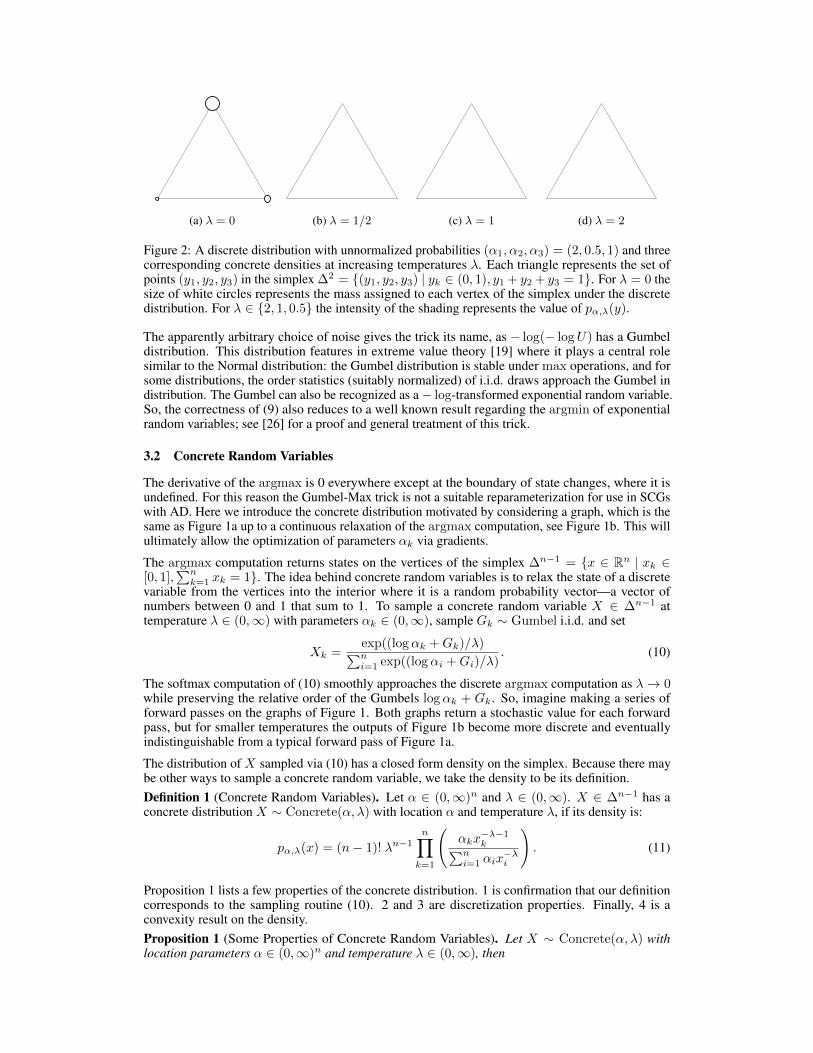
(a) λ = 0 (b) λ = 1/2 (c) λ = 1 (d) λ = 2

Figure 2: A discrete distribution with unnormalized probabilities (α1, α2, α3) = (2, 0.5, 1) and threecorresponding concrete densities at increasing temperatures λ. Each triangle represents the set ofpoints (y1, y2, y3) in the simplex ∆2 = {(y1, y2, y3) | yk ∈ (0, 1), y1 + y2 + y3 = 1}. For λ = 0 thesize of white circles represents the mass assigned to each vertex of the simplex under the discretedistribution. For λ ∈ {2, 1, 0.5} the intensity of the shading represents the value of pα,λ(y).

The apparently arbitrary choice of noise gives the trick its name, as − log(− logU) has a Gumbeldistribution. This distribution features in extreme value theory [19] where it plays a central rolesimilar to the Normal distribution: the Gumbel distribution is stable under max operations, and forsome distributions, the order statistics (suitably normalized) of i.i.d. draws approach the Gumbel indistribution. The Gumbel can also be recognized as a− log-transformed exponential random variable.So, the correctness of (9) also reduces to a well known result regarding the argmin of exponentialrandom variables; see [26] for a proof and general treatment of this trick.

3.2 Concrete Random Variables

The derivative of the argmax is 0 everywhere except at the boundary of state changes, where it isundefined. For this reason the Gumbel-Max trick is not a suitable reparameterization for use in SCGswith AD. Here we introduce the concrete distribution motivated by considering a graph, which is thesame as Figure 1a up to a continuous relaxation of the argmax computation, see Figure 1b. This willultimately allow the optimization of parameters αk via gradients.

The argmax computation returns states on the vertices of the simplex ∆n−1 = {x ∈ Rn | xk ∈[0, 1],

∑nk=1 xk = 1}. The idea behind concrete random variables is to relax the state of a discrete

variable from the vertices into the interior where it is a random probability vector—a vector ofnumbers between 0 and 1 that sum to 1. To sample a concrete random variable X ∈ ∆n−1 attemperature λ ∈ (0,∞) with parameters αk ∈ (0,∞), sample Gk ∼ Gumbel i.i.d. and set

Xk =exp((logαk +Gk)/λ)∑ni=1 exp((logαi +Gi)/λ)

. (10)

The softmax computation of (10) smoothly approaches the discrete argmax computation as λ→ 0while preserving the relative order of the Gumbels logαk + Gk. So, imagine making a series offorward passes on the graphs of Figure 1. Both graphs return a stochastic value for each forwardpass, but for smaller temperatures the outputs of Figure 1b become more discrete and eventuallyindistinguishable from a typical forward pass of Figure 1a.

The distribution of X sampled via (10) has a closed form density on the simplex. Because there maybe other ways to sample a concrete random variable, we take the density to be its definition.Definition 1 (Concrete Random Variables). Let α ∈ (0,∞)n and λ ∈ (0,∞). X ∈ ∆n−1 has aconcrete distribution X ∼ Concrete(α, λ) with location α and temperature λ, if its density is:

pα,λ(x) = (n− 1)! λn−1n∏k=1

(αkx

−λ−1k∑n

i=1 αix−λi

). (11)

Proposition 1 lists a few properties of the concrete distribution. 1 is confirmation that our definitioncorresponds to the sampling routine (10). 2 and 3 are discretization properties. Finally, 4 is aconvexity result on the density.Proposition 1 (Some Properties of Concrete Random Variables). Let X ∼ Concrete(α, λ) withlocation parameters α ∈ (0,∞)n and temperature λ ∈ (0,∞), then

(a) λ = 0 (b) λ = 1/2 (c) λ = 1 (d) λ = 2

Figure 3: A visualization of a Gumbel-Max reparameterization for Bernoulli random variables andsome corresponding concrete relaxations. (a) shows the discrete trick, which works by passing anoisy logit through the unit step function. (b), (c), (d) show concrete relaxations; the horizontal bluedensities show the density of the noise distribution L + logα and the vertical densities show thecorresponding concrete density over the interval (0, 1) of the random variable σ((L+ logα)/λ) forvarying temperatures λ.

1. (Reparameterization) If Gk ∼ Gumbel i.i.d., then Xkd= exp((logαk+Gk)/λ)∑n

i=1 exp((logαi+Gi)/λ),

2. (Rounding) P (Xk > Xi for i 6= k) = αk/(∑ni=1 αi),

3. (Zero temperature) P (limλ→0Xk = 1) = αk/(∑ni=1 αi),

4. (Convex eventually) If λ ≤ (n− 1)−1, then pα,λ(x) is log-convex in x.

We prove these results in the Appendix. There is an obvious question whether the Gumbel noise is anecessary feature of this idea. In the binary case, see Figure 3, it can be generalized to accommodateany additive noise distribution with infinite support (we cover this in the Appendix). In contrast, forthe general n-ary case the Gumbel is a crucial 1 and the Gumbel-Max trick cannot be generalized forother additive noise distributions [45]. In the Appendix we include a cheat sheet for all of the randomvariables we include in this work along with details on their implementation.

3.3 Concrete Random Variables as Relaxations

Concrete random variables may have some intrinsic value, but we investigate them simply assurrogates for optimizing a SCG with discrete nodes. When it is computationally feasible to integrateover the discreteness, that will always be a better choice. Otherwise the basic idea is to optimizea graph with every discrete stochastic node replaced by a concrete stochastic node at some fixedtemperature (or with an annealing schedule). Because the graphs are identical up to softmax /argmax computations, the parameters of the relaxed graph and discrete graph are the same. Thesuccess of concrete relaxations will depend heavily on the choice of temperature during training. It isimportant that the relaxed nodes are not able to represent a precise real valued mode in the interiorof the simplex as in Figure 2d. If this is the case, it is possible for the relaxed random variable tocommunicate much more than log2(n) bits of information about its α parameters. This might leadthe relaxation to prefer the interior of the simplex to the vertices, and as a result there will be a largeintegrality gap in the overall performance of the discrete graph. Therefore 4 of Proposition 1 is aconservative guideline for generic n-ary concrete relaxations; at temperatures lower than (n− 1)−1

we are guaranteed not to have any modes in the interior for any α ∈ (0,∞)n. We discuss thesubtleties of choosing the temperature in more detail in the Appendix. Ultimately the best choice ofλ and the performance of the relaxation for any specific n will be an empirical question.

When an objective depends on the log-probability of discrete variables in the SCG, as the variationallowerbound does, we must consider how to modify it in the context of a relaxation. To preservethe property that the variational objective bounds the log-probability of the observed data, the log-probability terms for the latent variables must match their sampling distribution. Thus, in additionto relaxing the sampling pass of a SCG the log-probability terms are also “relaxed” to represent thetrue distribution of the relaxed node. One could treat the Gumbels Gk as the stochastic node, andthe softmax as downstream computation. However, this is a looser bound than the bound dependingon log-probability of the concrete states in the simplex, because the softmax is many-to-one. Thus,the concrete-discrete pairing satisfies this valuable property: the discretization of any concretedistribution has a closed form mass function, and the relaxation of any discrete distribution into aconcrete distribution has a closed form density. It is generally easy to go from a continuous processto a discrete one by quantizing and backwards by relaxing, but maintaining analytic tractability

both ways is not always possible. For example, there is no closed form for the mass function of themultinomial probit model — the Gumbel-Max trick but with Gaussians replacing Gumbels.

4 Related Work

Perhaps the most common distribution over the simplex is the Dirichlet with density pα(x) ∝∏nk=1 x

αk−1k on x ∈ ∆n−1. The Dirichlet can be characterized by strong independence properties,

and a great deal of work has been done to generalize it [7, 2, 34, 8]. Of note is the logistic Normaldistribution [3], which can be simulated by taking the softmax of n − 1 normal random variablesand an nth logit that is deterministically zero. The logistic Normal is an important distribution,because it can effectively model correlations within the simplex [5]. To our knowledge the concretedistribution does not fall completely into any family of distributions previously described. For λ ≤ 1the concrete is a member of a class of normalized infinitely divisible distributions (S. Favaro, personalcommunication), and the results of [8] apply.

The idea of using a softmax of Gumbels as a relaxation for a discrete random variable was concurrentlyconsidered by [21], where it was called the Gumbel-Softmax. They do not mention whether they usedthe density in the relaxed objective, opting instead to work with a vector of Gumbels passed througha softmax would result in a looser bound. The idea of using sigmoidal functions with additive inputnoise to approximate discreteness is also not a new idea. [9] introduced nonlinear Gaussian unitswhich computed their activation by passing Gaussian noise with the mean and variance specified bythe input to the unit through a nonlinearity, such as the logistic function. (author?) [37] binarizedreal-valued codes of an autoencoder by adding (Gaussian) noise to the logits before passing themthrough the logistic function. Most recently, to avoid the difficulty associated with likelihood-ratiomethods [25] relaxed the discrete sampling operation by sampling a vector of Gaussians and passingit through a softmax instead.

There is another family of gradient estimators that have been studied in the context of training neuralnetworks with discrete units. These are usually collected under the umbrella of straight-throughestimators [4, 32]. The basic idea they use is passing forward discrete values, but taking gradientsthrough the expected value. They have good empirical performance, but have not been shown to bethe estimators of any loss function. This is in contrast to gradients from concrete relaxations, whichare biased with respect to the discrete graph, but unbiased with respect to the continuous one.

5 Experiments

5.1 Protocol

The aim of these experiments is to evaluate the effectiveness of the gradients of concrete relaxationsfor optimizing SCGs with discrete nodes. We considered the tasks in [29]: structured output predictionand density estimation. Both tasks are difficult optimization problems involving fitting probabilitydistributions with hundreds of latent discrete nodes. We compare the performance of concretereparameterizations to two state-of-the-art score function estimators: VIMCO [29] for optimizingthe multisample variational objective (m > 1) and NVIL [28] for optimizing the single-sample one(m = 1). We report the negative log-likelihood (NLL) of the discrete graph on the test data as theperformance metric. Appendix contains more experimental details.

All our models are neural networks with layers of n-ary discrete stochastic nodes with log2(n)-dimensional states on the corners of the hypercube {−1, 1}log2(n). The distribution of the nodesare parameterized by n real values logαk ∈ R, which we take to be the logits of a discrete randomvariable D ∼ Discrete(α) with n states. Model descriptions are of the form “(200V–200H∼784V)”,read from left to right. This describes the order of conditional sampling, again from left to right, witheach integer representing the number of stochastic units in a layer. The letters V and H representobserved and latent variables, respectively. If the leftmost layer is H, then it is sampled unconditionallyfrom some parameters. Conditioning functions are taken from {–, ∼}, where “–” means a linearfunction of the previous layer and “∼” means a non-linear function. A “layer” of these units issimply the concatenation of some number of independent nodes whose parameters are determinedas a function the previous layer. For example a 240 binary layer is a factored distribution overthe {−1, 1}240 hypercube. Whereas a 240 8-ary layer can be seen as a distribution over the same

MNIST NLL Omniglot NLL

binarymodel

Test Train Test Train

m Concrete VIMCO Concrete VIMCO Concrete VIMCO Concrete VIMCO

(200H– 784V)

1 107.3 104.4 107.5 104.2 118.7 115.7 117.0 112.25 104.9 101.9 104.9 101.5 118.0 113.5 115.8 110.850 104.3 98.8 104.2 98.3 118.9 113.0 115.8 110.0

(200H– 200H– 784V)

1 102.1 92.9 102.3 91.7 116.3 109.2 114.4 104.85 99.9 91.7 100.0 90.8 116.0 107.5 113.5 103.650 99.5 90.7 99.4 89.7 117.0 108.1 113.9 103.6

(200H∼784V)

1 92.1 93.8 91.2 91.5 108.4 116.4 103.6 110.35 89.5 91.4 88.1 88.6 107.5 118.2 101.4 102.350 88.5 89.3 86.4 86.5 108.1 116.0 100.5 100.8

(200H∼200H∼784V)

1 87.9 88.4 86.5 85.8 105.9 111.7 100.2 105.75 86.3 86.4 84.1 82.5 105.8 108.2 98.6 101.150 85.7 85.5 83.1 81.8 106.8 113.2 97.5 95.2

Table 1: Density estimation with binary latent variables and distinct models. When m = 1, VIMCOstands for NVIL.

hypercube where each of the 80 triples of units are sampled independently from an 8 way discretedistribution over {−1, 1}3. These models were initialized with the heuristic of [11] and optimizedusing Adam [22]. The Appendix contains the details of hyperparameter selection. For concreterelaxations the temperatures were fixed throughout training.

We performed the experiments using the MNIST and Omniglot datasets. These are datasets of28 × 28 images of handwritten digits (MNIST) or letters (Omniglot). For MNIST we used thefixed binarization of [38] and the standard 50,000/10,000/10,000 split into training/validation/testingsets. For Omniglot we sampled a fixed binarization and used the standard 24,345/8,070 split intotraining/testing sets.

5.2 Density Estimation

Density estimation, or generative modelling, is the problem of capturing the distribution of the databy fitting a probabilistic model to samples from this distribution . We will take the latent variablemodelling approach described in Section 2.4 and will train the models by optimizing the variationalobjective Lm(θ, φ) given by Eq. 8. Both our generative models pθ(z, x) and variational distributionsqφ(z | x) will be parameterized as belief networks as described above.

We trained models by optimizing Lm(θ, φ) for m ∈ {1, 5, 50} and computed the log-likelihoodestimates by evaluating L50,000(θ, φ). The results are shown in Table 1. In general, VIMCOoutperformed concrete relaxations for linear models and concrete relaxations outperformed VIMCOfor non-linear models. We also tested the effectiveness of concrete relaxations on generative modelswith n-ary layers on the L5(θ, φ) objective. The best 4-ary model achieved test/train NLL 86.7/83.3,the best 8-ary achieved 87.4/84.6 with concrete relaxations, more complete results in Appendix. Therelatively poor performance of the 8-ary model may be because moving from 4 to 8 results in amore difficult objective without much added capacity. As a control we trained n-ary models usinglogistic normals as relaxations of discrete distributions (with retuned temperature hyperparameters).Because the discrete zero temperature limit of logistic Normals is a multinomial probit whose massfunction is not known, to evaluate the discrete model we simply sampled from the discrete distributionparameterized in the traditional way by the logits learned during training. The best 4-ary modelachieved test/train NLL of 88.7/85.0, the best 8-ary model achieved 89.1/85.1.

5.3 Structured Output Prediction

Structured output prediction is concerned with modelling the high-dimensional distribution of theobservation given a context and can be seen as conditional density estimation. We will considerthe task of predicting the bottom half x1 of an image of an MNIST digit given its top half x2, asintroduced by [32]. As the problem is multimodal, we follow [32] in using a model with layers ofdiscrete stochastic units between the context and the observation. Conditioned on the top half x2 the

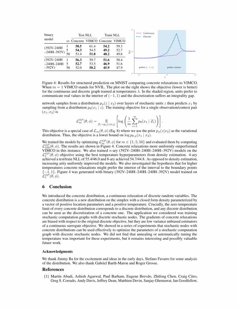
binarymodel

Test NLL Train NLL

m Concrete VIMCO Concrete VIMCO

(392V–240H–240H–392V)

1 58.5 61.4 54.2 59.35 54.3 54.5 49.2 52.750 53.4 51.8 48.2 49.6

(392V–240H–240H–240H–392V)

1 56.3 59.7 51.6 58.45 52.7 53.5 46.9 51.650 52.0 50.2 45.9 47.9

100 101 102

�

101

102

103

NLL

prefers interiorprefers {�1, 1}

Continuous

Discrete

Figure 4: Results for structured prediction on MNIST comparing concrete relaxations to VIMCO.When m = 1 VIMCO stands for NVIL. The plot on the right shows the objective (lower is better)for the continuous and discrete graph trained at temperatures λ. In the shaded region, units prefer tocommunicate real values in the interior of (−1, 1) and the discretization suffers an integrality gap.

network samples from a distribution pφ(z | x2) over layers of stochastic units z then predicts x1 bysampling from a distribution pθ(x1 | z). The training objective for a single observation/context pair(x1, x2) is

LSPm (θ, φ) = EZi∼pφ(z|x2)

[log

(1

m

m∑i=1

pθ(x1 | Zi))]

.

This objective is a special case of Lm(θ, φ) (Eq. 8) where we use the prior pφ(z|x2) as the variationaldistribution. Thus, the objective is a lower bound on log pθ,φ(x1 | x2).

We trained the models by optimizing LSPm (θ, φ) for m ∈ {1, 5, 50} and evaluated them by computingLSP100(θ, φ). The results are shown in Figure 4. Concrete relaxations more uniformly outperformedVIMCO in this instance. We also trained n-ary (392V–240H–240H–240H–392V) models on theLSP1 (θ, φ) objective using the best temperature hyperparameters from density estimation. 4-aryachieved a test/train NLL of 55.4/46.0 and 8-ary achieved 54.7/44.8. As opposed to density estimation,increasing arity uniformly improved the models. We also investigated the hypothesis that for highertemperatures concrete relaxations might prefer the interior of the interval to the boundary points{−1, 1}. Figure 4 was generated with binary (392V–240H–240H–240H–392V) model trained onLSP1 (θ, φ).

6 Conclusion

We introduced the concrete distribution, a continuous relaxation of discrete random variables. Theconcrete distribution is a new distribution on the simplex with a closed form density parameterized bya vector of positive location parameters and a positive temperature. Crucially, the zero temperaturelimit of every concrete distribution corresponds to a discrete distribution, and any discrete distributioncan be seen as the discretization of a concrete one. The application we considered was trainingstochastic computation graphs with discrete stochastic nodes. The gradients of concrete relaxationsare biased with respect to the original discrete objective, but they are low variance unbiased estimatorsof a continuous surrogate objective. We showed in a series of experiments that stochastic nodes withconcrete distributions can be used effectively to optimize the parameters of a stochastic computationgraph with discrete stochastic nodes. We did not find that annealing or automatically tuning thetemperature was important for these experiments, but it remains interesting and possibly valuablefuture work.

Acknowledgments

We thank Jimmy Ba for the excitement and ideas in the early days, Stefano Favarro for some analysisof the distribution. We also thank Gabriel Barth-Maron and Roger Grosse.

References[1] Martín Abadi, Ashish Agarwal, Paul Barham, Eugene Brevdo, Zhifeng Chen, Craig Citro,

Greg S. Corrado, Andy Davis, Jeffrey Dean, Matthieu Devin, Sanjay Ghemawat, Ian Goodfellow,

Andrew Harp, Geoffrey Irving, Michael Isard, Yangqing Jia, Rafal Jozefowicz, Lukasz Kaiser,Manjunath Kudlur, Josh Levenberg, Dan Mané, Rajat Monga, Sherry Moore, Derek Murray,Chris Olah, Mike Schuster, Jonathon Shlens, Benoit Steiner, Ilya Sutskever, Kunal Talwar, PaulTucker, Vincent Vanhoucke, Vijay Vasudevan, Fernanda Viégas, Oriol Vinyals, Pete Warden,Martin Wattenberg, Martin Wicke, Yuan Yu, and Xiaoqiang Zheng. TensorFlow: Large-scalemachine learning on heterogeneous systems, 2015. Software available from tensorflow.org.

[2] J Aitchison. A general class of distributions on the simplex. Journal of the Royal StatisticalSociety. Series B (Methodological), pages 136–146, 1985.

[3] J Atchison and Sheng M Shen. Logistic-normal distributions: Some properties and uses.Biometrika, 67(2):261–272, 1980.

[4] Yoshua Bengio, Nicholas Léonard, and Aaron Courville. Estimating or propagating gradientsthrough stochastic neurons for conditional computation. arXiv preprint arXiv:1308.3432, 2013.

[5] David Blei and John Lafferty. Correlated topic models. 2006.[6] Yuri Burda, Roger Grosse, and Ruslan Salakhutdinov. Importance weighted autoencoders.

ICLR, 2016.[7] Robert J Connor and James E Mosimann. Concepts of independence for proportions with a

generalization of the dirichlet distribution. Journal of the American Statistical Association,64(325):194–206, 1969.

[8] Stefano Favaro, Georgia Hadjicharalambous, and Igor Prünster. On a class of distributions onthe simplex. Journal of Statistical Planning and Inference, 141(9):2987 – 3004, 2011.

[9] Brendan Frey. Continuous sigmoidal belief networks trained using slice sampling. In NIPS,1997.

[10] Michael C Fu. Gradient estimation. Handbooks in operations research and management science,13:575–616, 2006.

[11] Xavier Glorot and Yoshua Bengio. Understanding the difficulty of training deep feedforwardneural networks. In Aistats, volume 9, pages 249–256, 2010.

[12] Peter W Glynn. Likelihood ratio gradient estimation for stochastic systems. Communicationsof the ACM, 33(10):75–84, 1990.

[13] Alex Graves, Greg Wayne, Malcolm Reynolds, Tim Harley, Ivo Danihelka, Agnieszka Grabska-Barwinska, Sergio Gómez Colmenarejo, Edward Grefenstette, Tiago Ramalho, John Agapiou,et al. Hybrid computing using a neural network with dynamic external memory. Nature,538(7626):471–476, 2016.

[14] Evan Greensmith, Peter L. Bartlett, and Jonathan Baxter. Variance reduction techniques forgradient estimates in reinforcement learning. JMLR, 5, 2004.

[15] Edward Grefenstette, Karl Moritz Hermann, Mustafa Suleyman, and Phil Blunsom. Learning totransduce with unbounded memory. In Advances in Neural Information Processing Systems,pages 1828–1836, 2015.

[16] Karol Gregor, Ivo Danihelka, Alex Graves, Danilo Jimenez Rezende, and Daan Wierstra. Draw:A recurrent neural network for image generation. arXiv preprint arXiv:1502.04623, 2015.

[17] Karol Gregor, Ivo Danihelka, Andriy Mnih, Charles Blundell, and Daan Wierstra. Deepautoregressive networks. arXiv preprint arXiv:1310.8499, 2013.

[18] Shixiang Gu, Sergey Levine, Ilya Sutskever, and Andriy Mnih. MuProp: Unbiased backpropa-gation for stochastic neural networks. ICLR, 2016.

[19] Emil Julius Gumbel. Statistical theory of extreme values and some practical applications: aseries of lectures. Number 33. US Govt. Print. Office, 1954.

[20] Matthew D Hoffman, David M Blei, Chong Wang, and John William Paisley. Stochasticvariational inference. JMLR, 14(1):1303–1347, 2013.

[21] E. Jang, S. Gu, and B. Poole. Categorical Reparameterization with Gumbel-Softmax. ArXive-prints, November 2016.

[22] Diederik Kingma and Jimmy Ba. Adam: A method for stochastic optimization. arXiv preprintarXiv:1412.6980, 2014.

[23] Diederik P Kingma and Max Welling. Auto-encoding variational bayes. arXiv preprintarXiv:1312.6114, 2013.

[24] Diederik P Kingma and Max Welling. Auto-encoding variational bayes. ICLR, 2014.

[25] Tomáš Kociský, Gábor Melis, Edward Grefenstette, Chris Dyer, Wang Ling, Phil Blunsom,and Karl Moritz Hermann. Semantic parsing with semi-supervised sequential autoencoders. InEMNLP, 2016.

[26] Chris J Maddison. A Poisson process model for Monte Carlo. arXiv preprint arXiv:1602.05986,2016.

[27] Chris J Maddison, Daniel Tarlow, and Tom Minka. A∗ Sampling. In NIPS, 2014.[28] Andriy Mnih and Karol Gregor. Neural variational inference and learning in belief networks. In

ICML, 2014.[29] Andriy Mnih and Danilo Jimenez Rezende. Variational inference for monte carlo objectives. In

ICML, 2016.[30] Christian A Naesseth, Francisco JR Ruiz, Scott W Linderman, and David M Blei. Rejection

sampling variational inference. arXiv preprint arXiv:1610.05683, 2016.[31] John William Paisley, David M. Blei, and Michael I. Jordan. Variational bayesian inference

with stochastic search. In ICML, 2012.[32] Tapani Raiko, Mathias Berglund, Guillaume Alain, and Laurent Dinh. Techniques for learning

binary stochastic feedforward neural networks. arXiv preprint arXiv:1406.2989, 2014.[33] Rajesh Ranganath, Sean Gerrish, and David M. Blei. Black box variational inference. In

AISTATS, 2014.[34] William S Rayens and Cidambi Srinivasan. Dependence properties of generalized liouville

distributions on the simplex. Journal of the American Statistical Association, 89(428):1465–1470, 1994.

[35] Danilo Jimenez Rezende, Shakir Mohamed, and Daan Wierstra. Stochastic backpropagationand approximate inference in deep generative models. In ICML, 2014.

[36] Francisco JR Ruiz, Michalis K Titsias, and David M Blei. The generalized reparameterizationgradient. arXiv preprint arXiv:1610.02287, 2016.

[37] Ruslan Salakhutdinov and Geoffrey Hinton. Semantic hashing. International Journal ofApproximate Reasoning, 50(7):969–978, 2009.

[38] Ruslan Salakhutdinov and Iain Murray. On the quantitative analysis of deep belief networks. InICML, 2008.

[39] John Schulman, Nicolas Heess, Theophane Weber, and Pieter Abbeel. Gradient estimationusing stochastic computation graphs. In NIPS, 2015.

[40] Theano Development Team. Theano: A Python framework for fast computation of mathematicalexpressions. arXiv e-prints, abs/1605.02688, May 2016.

[41] Michalis Titsias and Miguel Lázaro-Gredilla. Doubly stochastic variational bayes for non-conjugate inference. In Tony Jebara and Eric P. Xing, editors, ICML, 2014.

[42] Michalis Titsias and Miguel Lázaro-Gredilla. Local expectation gradients for black box varia-tional inference. In NIPS, 2015.

[43] Ronald J Williams. Simple statistical gradient-following algorithms for connectionist reinforce-ment learning. Machine learning, 8(3-4):229–256, 1992.

[44] Kelvin Xu, Jimmy Ba, Ryan Kiros, Kyunghyun Cho, Aaron Courville, Ruslan Salakhudinov,Rich Zemel, and Yoshua Bengio. Show, attend and tell: Neural image caption generation withvisual attention. In ICML, 2015.

[45] John I Yellott. The relationship between luce’s choice axiom, thurstone’s theory of comparativejudgment, and the double exponential distribution. Journal of Mathematical Psychology,15(2):109–144, 1977.

Appendix

Proof of Proposition 1

Let X ∼ Concrete(α, λ) with location parameters α ∈ (0,∞)n and temperature λ ∈ (0,∞).

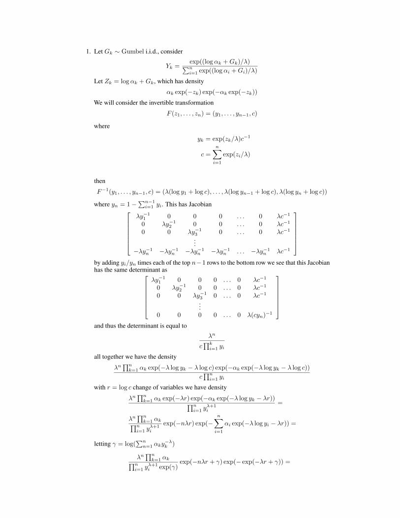
1. Let Gk ∼ Gumbel i.i.d., consider

Yk =exp((logαk +Gk)/λ)∑ni=1 exp((logαi +Gi)/λ)

Let Zk = logαk +Gk, which has density

αk exp(−zk) exp(−αk exp(−zk))

We will consider the invertible transformation

F (z1, . . . , zn) = (y1, . . . , yn−1, c)

where

yk = exp(zk/λ)c−1

c =

n∑i=1

exp(zi/λ)

then

F−1(y1, . . . , yn−1, c) = (λ(log y1 + log c), . . . , λ(log yn−1 + log c), λ(log yn + log c))

where yn = 1−∑n−1i=1 yi. This has Jacobian

λy−11 0 0 0 . . . 0 λc−1

0 λy−12 0 0 . . . 0 λc−1

0 0 λy−13 0 . . . 0 λc−1

...−λy−1n −λy−1n −λy−1n −λy−1n . . . −λy−1n λc−1

by adding yi/yn times each of the top n−1 rows to the bottom row we see that this Jacobianhas the same determinant as

λy−11 0 0 0 . . . 0 λc−1

0 λy−12 0 0 . . . 0 λc−1

0 0 λy−13 0 . . . 0 λc−1

...0 0 0 0 . . . 0 λ(cyn)−1

and thus the determinant is equal to

λn

c∏ki=1 yi

all together we have the density

λn∏nk=1 αk exp(−λ log yk − λ log c) exp(−αk exp(−λ log yk − λ log c))

c∏ni=1 yi

with r = log c change of variables we have density

λn∏nk=1 αk exp(−λr) exp(−αk exp(−λ log yk − λr))∏n

i=1 yλ+1i

=

λn∏nk=1 αk∏n

i=1 yλ+1i

exp(−nλr) exp(−n∑i=1

αi exp(−λ log yi − λr)) =

letting γ = log(∑nn=1 αky

−λk )

λn∏nk=1 αk∏n

i=1 yλ+1i exp(γ)

exp(−nλr + γ) exp(− exp(−λr + γ)) =

integrating out r

λn∏nk=1 αk∏n

i=1 yλ+1i exp(γ)

(exp(−γn+ γ)Γ(n)

λ

)=

λn−1∏nk=1 αk∏n

i=1 yλ+1i

(exp(−γn)Γ(n)) =

(n− 1)!λn−1∏nk=1 αky

−λ−1k

(∑nn=1 αky

−λk )n

Thus Y d= X .

2. Follows directly from 1 and the Gumbel-Max trick [26].

3. Follows directly from 1 and the Gumbel-Max trick [26].

4. Let λ ≤ (n− 1)−1. The density of X can be rewritten as

pα,λ(x) ∝n∏k=1

αky−λ−1∑n

i=1 αiy−λi

=

n∏k=1

αkyλ(n−1)−1k∑n

i=1 αi∏j 6=i y

λj

Thus, the log density is up to an additive constant C

log pα,λ(x) =

n∑k=1

(λ(n− 1)− 1) log yk − n log

n∑k=1

αk∏j 6=k

yλj

+ C

If λ ≤ (n− 1)−1, then the first n terms are convex, because − log is convex. For the lastterm, − log is convex and non-increasing and

∏j 6=k y

λj is concave for λ ≤ (n− 1)−1. Thus,

their composition is convex. The sum of convex terms is convex, finishing the proof.

Binary Gumbel-Max Trick

Bernoulli random variables are an important special case of discrete distributions. They take states in{0, 1}. Consider the binary version of the Gumbel-Max trick from Figure 1a. Let D ∼ Discrete(α)for α ∈ (0,∞)2 be that two state discrete random variable on {0, 1}2 parameterized as in Figure 1a.The distribution is degenerate, because D1 = 1−D2. Therefore we consider just D1. The event thatD1 = 1 is the event that {G1 + logα1 > G2 + logα2} where Gk ∼ Gumbel. The difference of twoGumbels is a Logistic distribution. L ∼ Logistic has the logistic function σ(x) = 1/(1 + exp(−x))

for a CDF. Therefore, L d= logU − log(1− U) where U ∼ Uniform(0, 1). If α = α1/α2 we have

ultimately,

P(D1 = 1) = P(G1 + logα1 > G2 + logα2) = P(L+ logα > 0)

Thus, D1d= H(logα+ logU − log(1− U)), where H is the unit step function.

To generalize this consider an arbitrary random variable X with infinite support on R. If Φ : R→[0, 1] is the CDF of X , then

P(H(X) = 1) = 1− Φ(0)

If we want this to have a Bernoulli distribution with probability α/(1 + α), then we should solve theequation

1− Φ(0) =α

1 + α.

This gives Φ(0) = 1/(1 + α), which can be accomplished by relocating the random variable Y withCDF Φ to be X = Y − Φ−1(1/(1 + α)).

Implementation Details for Concrete Distributions

In this section we include some tips for implementing and using the concrete distribution. We use thefollowing notation

σ(x) =1

1 + exp(−x)

n

LΣEk=1{xk} = log

(n∑k=1

exp(xk)

)Both sigmoid and log-sum-exp are common operations in libraries like TensorFlow or theano.

Which random variable to treat as the stochastic node. There can be numerical issues when workingwith concrete random variables, if they are implemented naively. When implementing a SCG likea variational autoencoder the question arises as to which part of the graph to treat as the stochasticnode on which log-likelihood terms are computed. It’s tempting in the case of concrete randomvariables to treat the Gumbels as the stochastic node on which the log-likelihood terms are evaluatedand the softmax as downstream computation. This will be a looser bound in the context of variationalinference than the corresponding bound when treating the concrete relaxed states as the node. Treatingthe concrete random variables as the stochastic nodes can lead to underflow then log of 0 issues.Outside of generic underflow/overflow issues when computing with softmaxes, is important toconsider these issues when implementing a generic drop-in distribution class.

The solution we found to work well was to consider the following vector in Rn for location parametersα ∈ (0,∞)n and λ ∈ (0,∞) and Gk ∼ Gumbel,

Yk =logαk +Gk

λ−

n

LΣEi=1

{logαi +Gi

λ

}Y ∈ Rn has the property that exp(Y ) ∼ Concrete(α, λ), therefore we call Y an ExpConcrete(α, λ).The advantage of this reparameterization is that the KL terms of a variational loss are invariant underinvertible transformation. exp is invertible, so the KL between two expconcrete random variablesis the same as the KL between two concrete random variables. The log-density log pα,λ(y) of anExpConcrete(α, λ) is also simple to compute:

log pα,λ(y) = log((n− 1)!) + (n− 1) log λ+

(n∑k=1

logαk − λyk)− n

n

LΣEk=1{logαk − λyk}

for y ∈ Rn such that LΣEnk=1{yk} = 0. Therefore, we used ExpConcrete random variables as thestochastic nodes and treated exp as a downstream computation. This has the additional advantage thatit can also represent the discrete limit. In the limit of λ→ 0 ExpConcrete random variables becomediscrete random variables over the one-hot vectors of d ∈ {−∞, 0}n where LΣEnk=1{dk} = 0, andfollowing this with exp results in the traditional one-hot vectors in {0, 1}n.

In the binary case, the logistic function is invertible, so it makes most sense to treat the logit plusnoise as the stochastic node. In particular, the binary random node was sample from:

X =logα+ logU − log(1− U)

λ

where U ∼ Uniform(0, 1) and always followed by σ as downstream computation. logU−log(1−U)is a logistic random variable, details in the cheat sheet, and so the log-density log pα,λ(x) of thisnode (before applying σ) is

log pα,λ(x) = log λ− λx+ µ− 2 log(1 + exp(−λx+ µ))

Choosing the temperature. The success of concrete relaxations will depend heavily on the choice oftemperature during training. It is important that the relaxed nodes are not able to represent a precisereal valued mode in the interior of the simplex as in Figure 2d. For example, choosing additiveGaussian noise ε ∼ Normal(0, 1) with the logistic function σ(x) to get relaxed Bernoullis of theform σ(ε + µ) will result in a large mode in the centre of the interval. This is because the tails ofthe Gaussian distribution drop off much faster than the rate at which σ squashes. Even including atemperature parameter does not completely solve this problem; the density of σ((ε+ µ)/λ) at anytemperature still goes to 0 as its approaches the boundaries 0 and 1 of the unit interval. Therefore 4of Proposition 1 is a conservative guideline for generic n-ary concrete relaxations; at temperatures

lower than (n− 1)−1 we are guaranteed not to have any modes in the interior for any α ∈ (0,∞)n.In the case of the binary concrete distribution, the tails of the logistic additive noise are balancedwith the logistic squashing function and for temperatures λ ≤ 1 the density of the binary concretedistribution is log-convex for all parameters α, see Figure 3b. Still, practice will often disagree withtheory here. The peakiness of the concrete distribution increases with n, so much higher temperaturesare tolerated (usually necessary).

For n = 1 temperatures λ ≤ (n − 1)−1 is a good guideline. For n > 1 taking λ ≤ (n − 1)−1

is not necessarily a good guideline, although it will depend on n and the specific application. Asn → ∞ the concrete distribution becomes peakier, because the random normalizing constant∑nk=1 exp((logαk + Gk)/λ) grows. This means that practically speaking the optimization can

tolerate much higher temperatures than (n− 1)−1. We found in the cases n = 4 that λ = 1 was thebest temperature and in n = 8, λ = 2/3 was the best. Yet λ = 2/3 was the best single performingtemperature across the n ∈ {2, 4, 8} cases that we considered. We recommend starting in thatball-park and exploring for any specific application.

Experimental Details

— vs ∼. The conditioning functions we used were either linear or non-linear. Non-linear consisted oftwo tanh layers of the same size as the preceding stochastic layer in the computation graph.

n-ary layers. All our models are neural networks with layers of n-ary discrete stochastic nodeswith log2(n)-dimensional states on the corners of the hypercube {−1, 1}log2(n). For a generic n-arynode sampling proceeds as follows. Sample a n-ary discrete random variable D ∼ Discrete(α) forα ∈ (0,∞)n. If C is the log2(n)× n matrix, which lists the corners of the hypercube {−1, 1}log2(n)

as columns, then we took Y = CD as downstream computation on D. The corresponding concreterelaxation is to take X ∼ Concrete(α, λ) for some fixed temperature λ ∈ (0,∞) and set Y =CX . For the binary case, this amounts to simply sampling U ∼ Uniform(0, 1) and taking Y =

2H(logU − log(1 − U) + logα) − 1. The corresponding binary concrete relaxation is Y =2σ((logU − log(1− U) + logα)/λ)− 1.

Bias initialization. All biases were initialized to 0 with the exception of the biases in the prior decoderdistribution over the 784 or 392 observed units. These were initialized to the logit of the base rateaveraged over the respective dataset (MNIST or Omniglot).

Centering. We also found it beneficial to center the layers of the inference network during training.The activity in (−1, 1)d of each stochastic layer was centered during training by maintaining aexponentially decaying average with rate 0.9 over minibatches. This running average was subtractedfrom the activity of the layer before it was updated. Gradients did not flow throw this computation, soit simply amounted to a dynamic offset. The averages were not updated during the evaluation.

Hyperparameter selection. All models were initialized with the heuristic of [11] and optimizedusing Adam [22] with parameters β1 = 0.9, β2 = 0.999 for 107 steps on minibatches of size 64.Hyperparameters were selected on the MNIST dataset by grid search taking the values that performedbest on the validation set. Learning rates were chosen from {10−4, 3 · 10−4, 10−3} and weight decayfrom {0, 10−2, 10−1, 1}. Two sets of hyperparameters were selected, one for linear models and onefor non-linear models. The linear models’ hyperparameters were selected with the 200H–200H–784Vdensity model on the L5(θ, φ) objective. The non-linear models’ hyperparameters were selectedwith the 200H∼200H∼784V density model on the L5(θ, φ) objective. For density estimation, theconcrete relaxation hyperparameters were (weight decay = 0, learning rate = 3 · 10−4) for linear and(weight decay = 0, learning rate = 10−4) for non-linear. For structured prediction concrete relaxationsused (weight decay = 10−3, learning rate = 3 · 10−4).

In addition to tuning learning rate and weight decay, we tuned temperatures for the concrete relaxationson the density estimation task. We found it valuable to have different values for the prior and posteriordistributions. In particular, for binary we found that (prior λ = 1/2, posterior λ = 2/3) was best, for4-ary we found (prior λ = 2/3, posterior λ = 1) was best, and (prior λ = 2/5, posterior λ = 2/3) for8-ary. No temperature annealing was used. For structured prediction we used just the correspondingposterior λ.

We performed early stopping when training with the score function estimators (VIMCO/NVIL) asthey were much more prone to overfitting.

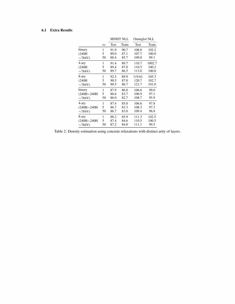
6.1 Extra Results

MNIST NLL Omniglot NLL

m Test Train Test Trainbinary(240H∼784V)

1 91.9 90.7 108.0 102.25 89.0 87.1 107.7 100.050 88.4 85.7 109.0 99.1

4-ary(240H∼784V)

1 91.4 89.7 110.7 1002.75 89.4 87.0 110.5 100.250 89.7 86.5 113.0 100.0

8-ary(240H∼784V)

1 92.5 89.9 119.61 105.35 90.5 87.0 120.7 102.750 90.5 86.7 121.7 101.0

binary(240H∼240H∼784V)

1 87.9 86.0 106.6 99.05 86.6 83.7 106.9 97.150 86.0 82.7 108.7 95.9

4-ary(240H∼240H∼784V)

1 87.4 85.0 106.6 97.85 86.7 83.3 108.3 97.350 86.7 83.0 109.4 96.8

8-ary(240H∼240H∼784V)

1 88.2 85.9 111.3 102.55 87.4 84.6 110.5 100.550 87.2 84.0 111.1 99.5

Table 2: Density estimation using concrete relaxations with distinct arity of layers.

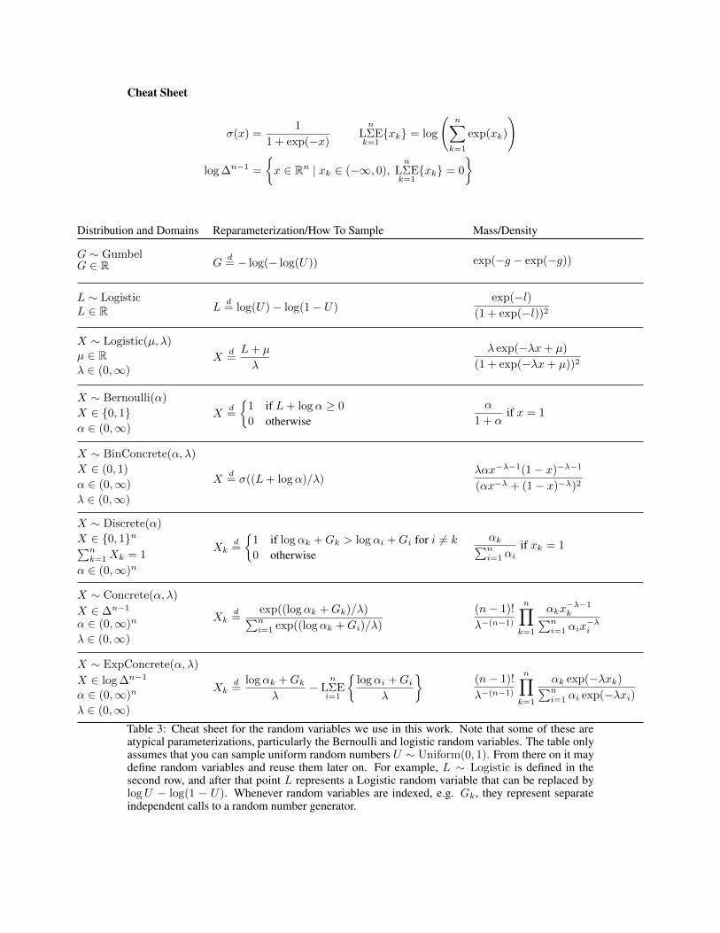
Cheat Sheet

σ(x) =1

1 + exp(−x)

n

LΣEk=1{xk} = log

(n∑k=1

exp(xk)

)

log ∆n−1 =

{x ∈ Rn | xk ∈ (−∞, 0),

n

LΣEk=1{xk} = 0

}

Distribution and Domains Reparameterization/How To Sample Mass/Density

G ∼ GumbelG ∈ R G

d= − log(− log(U)) exp(−g − exp(−g))

L ∼ LogisticL ∈ R L

d= log(U)− log(1− U)

exp(−l)(1 + exp(−l))2

X ∼ Logistic(µ, λ)µ ∈ Rλ ∈ (0,∞)

Xd=L+ µ

λ

λ exp(−λx+ µ)

(1 + exp(−λx+ µ))2

X ∼ Bernoulli(α)

X ∈ {0, 1}α ∈ (0,∞)

Xd=

{1 if L+ logα ≥ 0

0 otherwiseα

1 + αif x = 1

X ∼ BinConcrete(α, λ)

X ∈ (0, 1)

α ∈ (0,∞)

λ ∈ (0,∞)

Xd= σ((L+ logα)/λ)

λαx−λ−1(1− x)−λ−1

(αx−λ + (1− x)−λ)2

X ∼ Discrete(α)

X ∈ {0, 1}n∑nk=1Xk = 1

α ∈ (0,∞)n

Xkd=

{1 if logαk +Gk > logαi +Gi for i 6= k

0 otherwise

αk∑ni=1 αi

if xk = 1

X ∼ Concrete(α, λ)

X ∈ ∆n−1

α ∈ (0,∞)n

λ ∈ (0,∞)

Xkd=

exp((logαk +Gk)/λ)∑ni=1 exp((logαk +Gi)/λ)

(n− 1)!

λ−(n−1)

n∏k=1

αkx−λ−1k∑n

i=1 αix−λi

X ∼ ExpConcrete(α, λ)

X ∈ log ∆n−1

α ∈ (0,∞)n

λ ∈ (0,∞)

Xkd=

logαk +Gkλ

−n

LΣEi=1

{logαi +Gi

λ

}(n− 1)!

λ−(n−1)

n∏k=1

αk exp(−λxk)∑ni=1 αi exp(−λxi)

Table 3: Cheat sheet for the random variables we use in this work. Note that some of these areatypical parameterizations, particularly the Bernoulli and logistic random variables. The table onlyassumes that you can sample uniform random numbers U ∼ Uniform(0, 1). From there on it maydefine random variables and reuse them later on. For example, L ∼ Logistic is defined in thesecond row, and after that point L represents a Logistic random variable that can be replaced bylogU − log(1 − U). Whenever random variables are indexed, e.g. Gk, they represent separateindependent calls to a random number generator.