the compromise effect in action: lessons from a restaurant ...ftp.iza.org/dp9648.pdf · iza...

Forschungsinstitut zur Zukunft der ArbeitInstitute for the Study of Labor

DI

SC

US

SI

ON

P

AP

ER

S

ER

IE

S

The Compromise Effect in Action:Lessons from a Restaurant’s Menu

IZA DP No. 9648

January 2016

Pia PingerIsabel Ruhmer-KrellHeiner Schumacher

The Compromise Effect in Action: Lessons from a Restaurant’s Menu

Pia Pinger University of Bonn

and IZA

Isabel Ruhmer-Krell PricewaterhouseCoopers AG

Heiner Schumacher

KU Leuven

Discussion Paper No. 9648 January 2016

IZA

P.O. Box 7240 53072 Bonn

Germany

Phone: +49-228-3894-0 Fax: +49-228-3894-180

E-mail: [email protected]

Any opinions expressed here are those of the author(s) and not those of IZA. Research published in this series may include views on policy, but the institute itself takes no institutional policy positions. The IZA research network is committed to the IZA Guiding Principles of Research Integrity. The Institute for the Study of Labor (IZA) in Bonn is a local and virtual international research center and a place of communication between science, politics and business. IZA is an independent nonprofit organization supported by Deutsche Post Foundation. The center is associated with the University of Bonn and offers a stimulating research environment through its international network, workshops and conferences, data service, project support, research visits and doctoral program. IZA engages in (i) original and internationally competitive research in all fields of labor economics, (ii) development of policy concepts, and (iii) dissemination of research results and concepts to the interested public. IZA Discussion Papers often represent preliminary work and are circulated to encourage discussion. Citation of such a paper should account for its provisional character. A revised version may be available directly from the author.

IZA Discussion Paper No. 9648 January 2016

ABSTRACT

The Compromise Effect in Action: Lessons from a Restaurant’s Menu*

The compromise effect refers to individuals’ tendency to choose intermediate options. Its existence has been demonstrated in a large number of hypothetical choice experiments. This paper uses field data from a specialties restaurant to investigate the existence and strength of the compromise effect in a natural environment. Despite the presence of many factors that potentially weaken the compromise effect (e.g., a very large choice set, the opportunity to choose familiar options), we find evidence for it both in descriptive statistics and regression analyses. Options which become a compromise after a change in the choice set gain on average five percent in market share. We also find that the compromise effect is especially pronounced in groups, while for single customers it is statistically insignificant. JEL Classification: D03, M31 Keywords: utility theory, restaurant data, compromise effect Corresponding author: Pia Pinger Department of Economics University of Bonn Adenauerallee 24-42 53113 Bonn Germany E-mail: [email protected]

* The authors thank Dirk Engelmann, Johannes Koenen, Julian Krell, Christian Michel, Martin Peitz, Martin Watzinger and the seminar participants at the University of Mannheim for help and useful discussions. Anastasia Moor provided excellent research assistance. Isabel Ruhmer-Krell gratefully acknowledges financial support from the German Science Foundation (DFG). A first version of this paper was written while she was working at the University of Mannheim. Supplementary materials can be found in the Online Appendix.

https://docs.google.com/viewer?a=v&pid=sites&srcid=ZGVmYXVsdGRvbWFpbnxwaWFwaW5nZXJ8Z3g6NGE1NjFiMGE2NTVjYzAyMw

1 Introduction

A crucial assumption of rational choice theory is that decision makers have well-de�ned preferences

over all available options. It implies that a change in the composition of the choice set should not

a�ect the decision maker's preferences over two alternatives. However, a large body of work in

psychology and economics shows that this assumption is frequently violated. In many situations,

the context matters for choice behavior, i.e., the choice between two alternatives depends on which

other options are available. One of the most well-known context e�ects is the �compromise e�ect.�

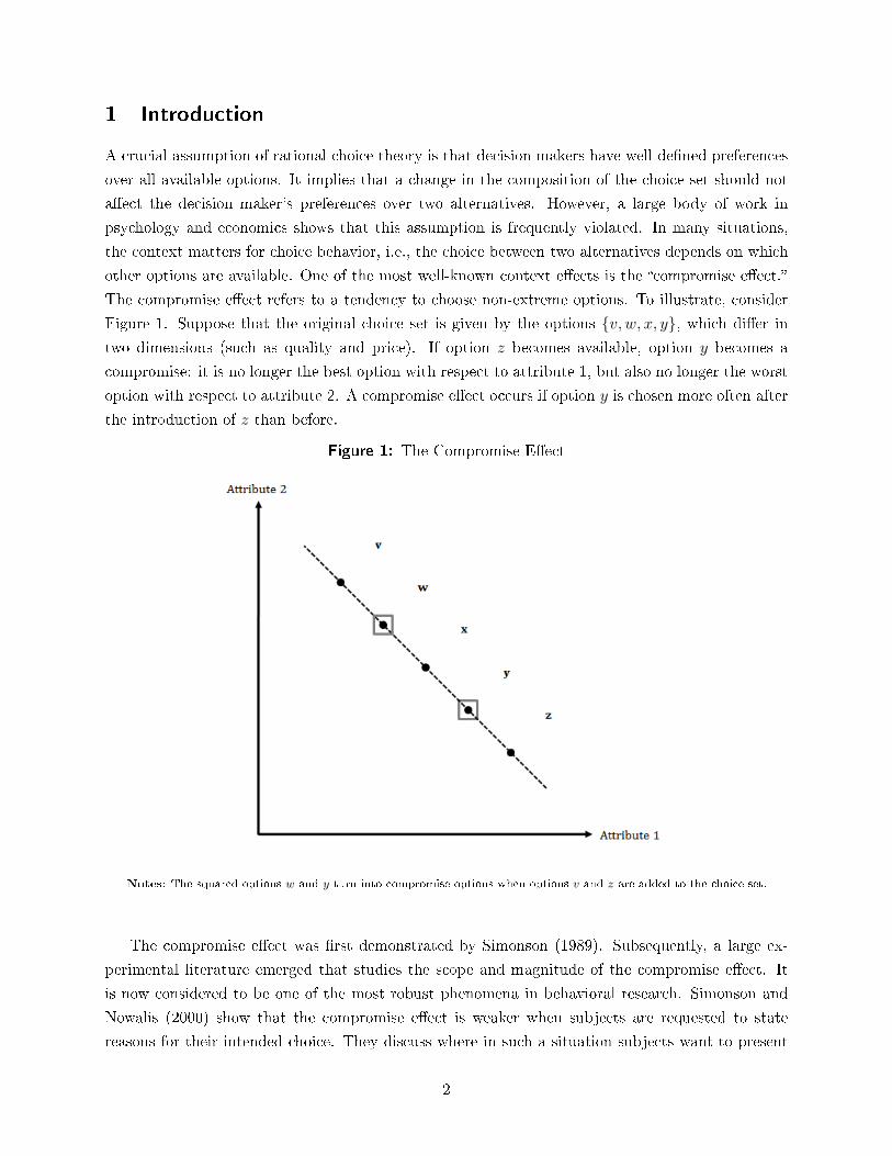
The compromise e�ect refers to a tendency to choose non-extreme options. To illustrate, consider

Figure 1. Suppose that the original choice set is given by the options {v, w, x, y}, which di�er in

two dimensions (such as quality and price). If option z becomes available, option y becomes a

compromise: it is no longer the best option with respect to attribute 1, but also no longer the worst

option with respect to attribute 2. A compromise e�ect occurs if option y is chosen more often after

the introduction of z than before.

Figure 1: The Compromise E�ect

Notes: The squared options w and y turn into compromise options when options v and z are added to the choice set.

The compromise e�ect was �rst demonstrated by Simonson (1989). Subsequently, a large ex-

perimental literature emerged that studies the scope and magnitude of the compromise e�ect. It

is now considered to be one of the most robust phenomena in behavioral research. Simonson and

Nowalis (2000) show that the compromise e�ect is weaker when subjects are requested to state

reasons for their intended choice. They discuss where in such a situation subjects want to present

2

reasons (and thus choices) that are less conventional. Dhar et al. (2000) demonstrate that time

pressure reduces the extent of the compromise e�ect. Dhar and Simonson (2003) �nd that introduc-

ing a �no-choice� option weakens or even eliminates the compromise e�ect. They conjecture that a

compromise is chosen especially by those subjects who are uncertain about their preferences. These

subjects are more likely to choose the no-choice option than subjects who select extreme options.

Similarly, Sheng et al. (2005) �nd that subjects who are more familiar with a product category

are less likely to choose the compromise. Kivetz et al. (2004a) demonstrate that the compromise

e�ect also prevails in larger choice sets with complex alternatives characterized by more than two

attributes. Chuang et al. (2012) investigate how recommendations of others a�ect the extent of

the compromise e�ect. They �nd that it is weaker when extreme options are recommended to the

decision maker. All of these papers use data from hypothetical choice experiments.

In this paper, we examine the compromise e�ect for the �rst time in a natural environment.

Speci�cally, we use the cashier data from a German specialties restaurant from a seven-year period.

They contain more than 88,000 individual choices. In the restaurant's menu, main dishes are

grouped into six categories (such as �sh, steaks, etc.). For each category, the options are listed

in an ascending-price order. During the observational period, the restaurant changed its menu

several times, thereby creating in each category choice set variations that can be used to study the

compromise e�ect.

The considered setting is clearly not conducive for the compromise e�ect. The customers of the

specialties restaurant may invest more cognitive e�ort into decisions than subjects in hypothetical

choice experiments. This may reduce the scope for decision biases (Levitt and List 2007). Moreover,

the choice situation � selecting a dish from a restaurant's menu � should be a familiar one to

most customers. In addition, all the mentioned sources of in�uence that potentially weaken the

compromise e�ect are present in our setting: there are many more options on the menu than in the

experiments cited above, and there are at least four choices in each food category; customers can

pick from categories they know well (e.g., they can choose a well-known dish); no-choice is an option;

and when customers arrive in groups, they may discuss their choices or make recommendations to

each other.

Despite these adverse factors, we �nd a signi�cant compromise e�ect in our data, both in

descriptive and regression analyses. On average, it amounts to an increase in market shares of

around �ve percentage points. However, its strength greatly varies between the di�erent food

categories, ranging from zero to over one hundred percent. Moreover, we �nd suggestive evidence

that the compromise e�ect is stronger for customers who dine in groups. For customers who dine

alone, we �nd no statistically signi�cant compromise e�ect.

Our results are relevant in at least two respects. First, they are of interest to theoretical re-

searchers, who aim at building empirically accurate models for economic choice behavior. Second,

they are important to practitioners and marketers, who may exploit the compromise e�ect to con-

struct choice sets strategically, so that the attractiveness and purchase likelihood of designated

high-margin options is maximized.

3

The paper contributes to several strands of the literature. A number of papers use behavioral

concepts to construct models that capture the compromise e�ect.1 Alternatively, one can explain

the compromise e�ect in a standard model by assuming that the choice set informs consumers about

important features of the environment (Wernerfelt 1995, Prelec et al. 1997, Kamenica 2008). The

propensity to choose middle options may be due to the fact that some consumers are uncertain

about their true preferences, but know that within the customer population they have intermediate

tastes. Our data do not allow us to examine the di�erent theories. However, the results provide

some support for the idea that the compromise e�ect is pronounced in product categories consumers

do not know well.

We also contribute to a growing literature that documents biased consumption choices using �eld

data and �eld experiments.2 Doyle et al. (1999) use sales data from a grocery store to show that the

attraction e�ect also occurs in a natural environment (the attraction e�ect refers to an increase in the

market share of an option when an alternative becomes available which is strictly dominated by that

option, but not by the other options in the original choice set). Iyengar and Lepper (2000) expose

shoppers in a grocery store to either limited choice sets (with 6 options) or extensive choice sets

(with 24 options). They demonstrate that the availability of too many options discourages choice

(�choice overload hypothesis�): Customers in the limited choice set condition were much more likely

to actually buy a product than customers in the extensive choice set condition. DellaVigna and

Malmendier (2006) analyze the customers' contract choice and attendance at three health clubs.

For a large share of customers a per-visit option would be optimal, given their realized attendance.

Nevertheless, many of them purchase costly long-term contracts, which implies a monetary loss.

The authors show that these customers on average overestimate future attendance when signing the

contract. Abeler and Marklein (2015) randomly distribute cash grants and in-kind grants (vouchers

1Simonson and Tversky (1992) argue that it may be due to �extremeness aversion�: Unlike extreme options,compromise options � such as options w and y in Figure 1 when the choice set is {v, w, x, y, z} � have no largedisadvantages. When disadvantages are weighted more than advantages (as under loss aversion), this feature makescompromises attractive. Tversky and Simonson (1993) derive the compromise e�ect from a simple utility frameworkthat exhibits two non-standard features, �background� and �choice set� e�ects. Background (e.g., previous exposureto other choice sets) in�uences the weight of each dimension in the utility function; the choice set in�uences thevaluation of an option through pairwise comparisons of this option with the alternatives in the choice set. Kivetzet al. (2004a) build four context-dependent choice models, which they estimate and test using experimental data.In particular, they show that these models can better explain the data than traditional choice models that arederived from value maximization. Kivetz et al. (2004b) discuss to what extent their models can be extended to morecomplex environments, such as group decisions or the purchase of complex products. De Clippel and Eliaz (2012)construct a multiple selves model in which both the compromise and the attraction e�ect occur as a solution of abargaining game between di�erent selves, which represent the di�erent quality dimensions. There is also a growingliterature on non-standard choice theory that captures empirically relevant phenomena related to the compromisee�ect. Masatlioglu and Ok (2005) extend rational choice theory by a status quo bias. Rubinstein and Salant (2006)analyze rational choice from lists (rather than sets) where the order of presentation potentially matters for decisions.Manzini and Mariotti (2007) and Apesteguia and Bellester (2013) examine multi-stage decision processes that canrationalize choices that violate the axiom of independence of irrelevant alternatives. In Ehlers and Sprumont (2008)and Lombardi (2008) choices are modeled as the outcome of a tournament, and thus may be cyclic (a fact knownas the Condorcet paradox). Salant and Rubinstein (2008) study choice functions that depend on the framing of theproblem.

2There are many more studies on biases in �nancial decision making and labor economics; see DellaVigna (2009)and List and Rasul (2010) for reviews.

4

for beverages) to customers in a restaurant. They �nd that consumers do not treat these grants as

fungible. Instead, they change consumption according to the label of the in-kind grant.

The remainder of this paper is organized as follows. Section 2 formally derives the di�erent

measures for the strength of the compromise e�ect which are commonly used in the literature.

Section 3 describes the data set and our empirical strategy. Our results are discussed in Section 4.

Section 5 concludes.

2 Theoretical Framework

This section de�nes the notion of the compromise e�ect within the standard choice framework and

derives implications that can be tested with aggregate data.3 Let T be the set of all potential

options. Each option x ∈ T has n attributes such as price, taste or quality. Let xi be the score

of option x in dimension i. A choice function C(S) assigns to every set S ⊂ T an option that the

decision maker chooses (for convenience, we rule out that the decision maker is indi�erent between

two or more options). A choice function C satis�es �value maximization� if there exists a function

v : T → R that assigns a real value to each option so that x = C(S) if and only if v(x) ≥ v(y) for

all y ∈ S.An immediate consequence of value maximization is the �independence of irrelevant alternatives�

(IIA). An option that is not chosen cannot become the chosen option when new options are added to

the choice set. Formally, this means that x = C(T ) and x ∈ S ⊂ T imply x = C(S). Unfortunately,

it is impossible to detect a violation of IIA in aggregate data. The ordering of market shares of two

options x and y may reverse under value maximization when a new option becomes available.4 We

therefore examine the implications of value maximization for the market share of an option under

varying choice sets.

A second consequence of value maximization is �regularity�: The market share of an option x

cannot increase when new options are added to the choice set. De�ne by P (x;T ) the market share

of option x if the choice set is given by T , and by P (S;T ) the sum market shares of the options in

S ⊂ T if the choice set is T . Regularity then means that x ∈ S ⊂ T implies P (x;S) ≥ P (x;T ).

This inequality is most commonly used to detect violations of value maximization. In particular,

the di�erence ∆P1(x) = P (x;T )− P (x;S) is used as a measure for the compromise e�ect.

There exists yet another implication of value maximization for aggregate data, but it requires

stronger assumptions on the value function v. Suppose that v is de�ned over an option's attributes,

v(x) = v(x1, ..., xn), and that it continuously increases in each attribute. We say that option y �lies

in between option x and z� if its attribute scores are such that xi ≤ yi ≤ zi for each dimension i.

3In this section, we follow and extend the framework of Tversky and Simonson (1993).4To illustrate, assume that x is chosen more often than y when only these two options are available. Now add

option z to the choice set. The ordering of market shares of x and y reverses if those consumers who originally chosex strictly prefer z to x, while those consumers who originally chose y strictly prefer y to z.

5

De�ne the �popularity� of y relative to x in the choice set S by

P (y, x;S) =P (y;S)

P (y;S) + P (x;S).

Under an additional weak assumption � the �ranking condition� � option y loses relatively more in

terms of market share than option x when z is introduced.5 To capture this formally, de�ne by

S and T two choice sets where T = S ∪ {z}. If the ranking condition and value maximization is

satis�ed, then y lying in between x and z implies P (y, x;S) ≥ P (y, x;T ). The di�erence ∆P2(y) =

P (y, x;T )− P (y, x;S) therefore is our second measure for the compromise e�ect. If there are more

than two options in set S, measure ∆P2 can be de�ned for all options x with xi ≤ yi in each

dimension i. We construct a third measure for the compromise e�ect that uses this fact. Denote by

S− y the set that contains all options from S except y and assume that for each option x ∈ S− y itholds that y lies between x and z. Then value maximization and the ranking condition imply that

P (y, S− y;S) ≥ P (y, S− y;T ). The di�erence ∆P3(y) = P (y, S− y;T )−P (y, S− y;S) is then our

third measure for the compromise e�ect.

3 Data and Empirical Strategy

3.1 Data

Our data originate from a German specialties restaurant located in a rural area of North-Eastern

Germany.6 According to the owner, at most 25 percent of customers visit the restaurant on a regular

basis (around once a month); all other customers are tourists who use the restaurant as a day-trip

destination.7

The restaurant provided two datasets. The �rst dataset includes all the restaurant's bills from

January 5, 2002 until May 29, 2009. They contain 88,113 individual choices of main dishes. We

can, in addition, extract the amount and prices of dishes ordered, the total billing amount, date

and time, table number and the name of the waiter.

The second dataset is the menus that were o�ered to customers during the observational period.

In total, there were 21 di�erent menus. Each menu contains between 24 and 30 main dishes. These

were grouped into six separate categories: traditional, �sh, venison, steaks, poultry and vegetarian.

Within each category, the available dishes are listed according to price, starting with the cheapest

option. Figure 2 shows several examples. From these menus we can extract information about the

exact position of each item within each category.8

5See the Online Appendix for details.6The exact name and location is not disclosed in agreement with the restaurant's owner. Aggregation of the

available data could otherwise allow local competitors to take advantage of �nancial �gures.7This is supported by Table 1, which shows that 57% of all menu choices were made on weekends.8The categories remained the same over time even though the category names varied slightly (see Figure 2).

One dish (chicken breast �llet) was listed in two categories (poultry and steaks) in three menus. In those cases werandomly assigned half of the observations to each of the categories.

6


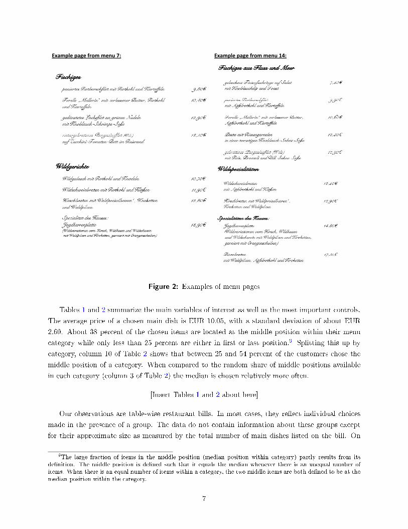
Example page from menu 7:

Example page from menu 14:

Figure 2: Examples of menu pages

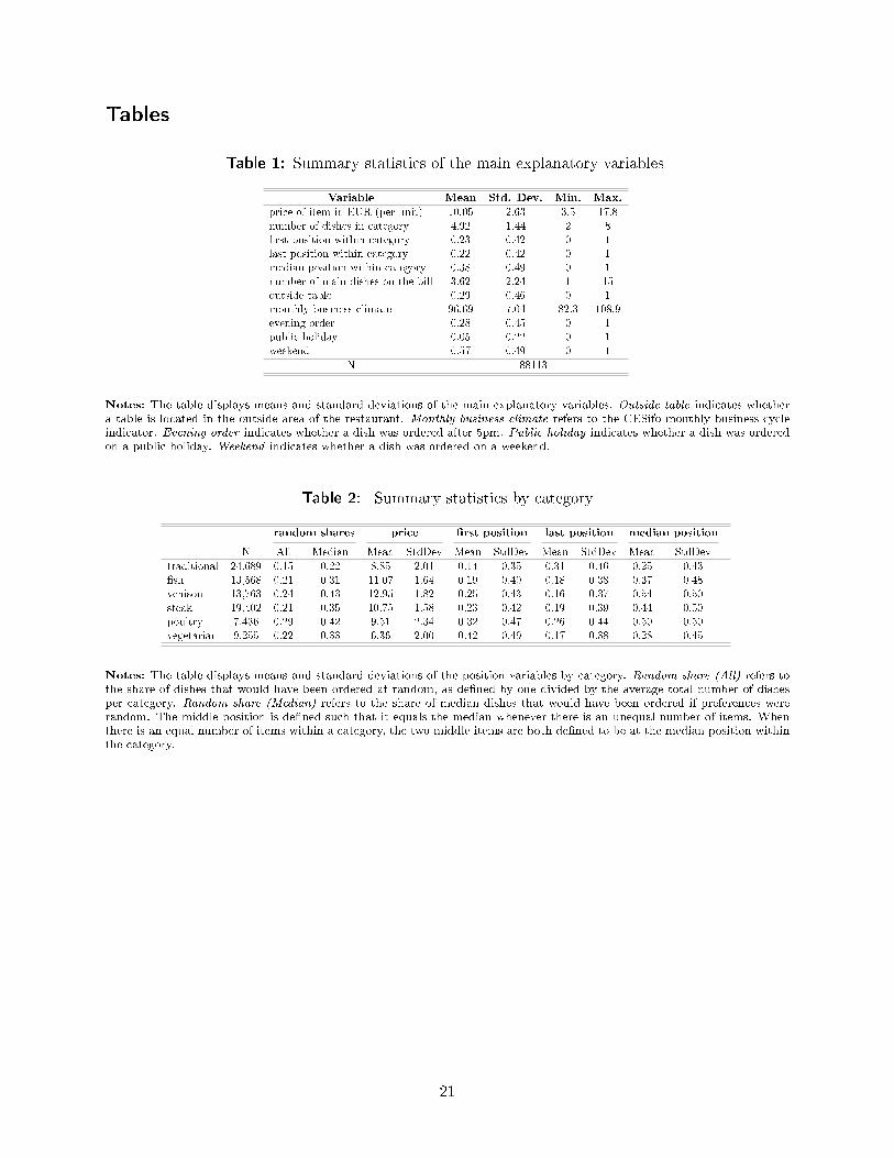
Tables 1 and 2 summarize the main variables of interest as well as the most important controls.

The average price of a chosen main dish is EUR 10.05, with a standard deviation of about EUR

2.60. About 38 percent of the chosen items are located at the middle position within their menu

category while only less than 25 percent are either in �rst or last position.9 Splitting this up by

category, column 10 of Table 2 shows that between 25 and 54 percent of the customers chose the

middle position of a category. When compared to the random share of middle positions available

in each category (column 3 of Table 2) the median is chosen relatively more often.

[Insert Tables 1 and 2 about here]

Our observations are table-wise restaurant bills. In most cases, they re�ect individual choices

made in the presence of a group. The data do not contain information about these groups except

for their approximate size as measured by the total number of main dishes listed on the bill. On

9The large fraction of items in the middle position (median position within category) partly results from itsde�nition. The middle position is de�ned such that it equals the median whenever there is an unequal number ofitems. When there is an equal number of items within a category, the two middle items are both de�ned to be at themedian position within the category.

7

average, individuals come in groups of three or four (the average number of main dishes per bill is

3.62). Only 7.13 percent of all bills contained a single main dish.

As control variables we use regional weather data on the average daily temperature, macroeco-

nomic indicators on the monthly unemployment rate at the district level, and an index measuring

the business climate on the national level.

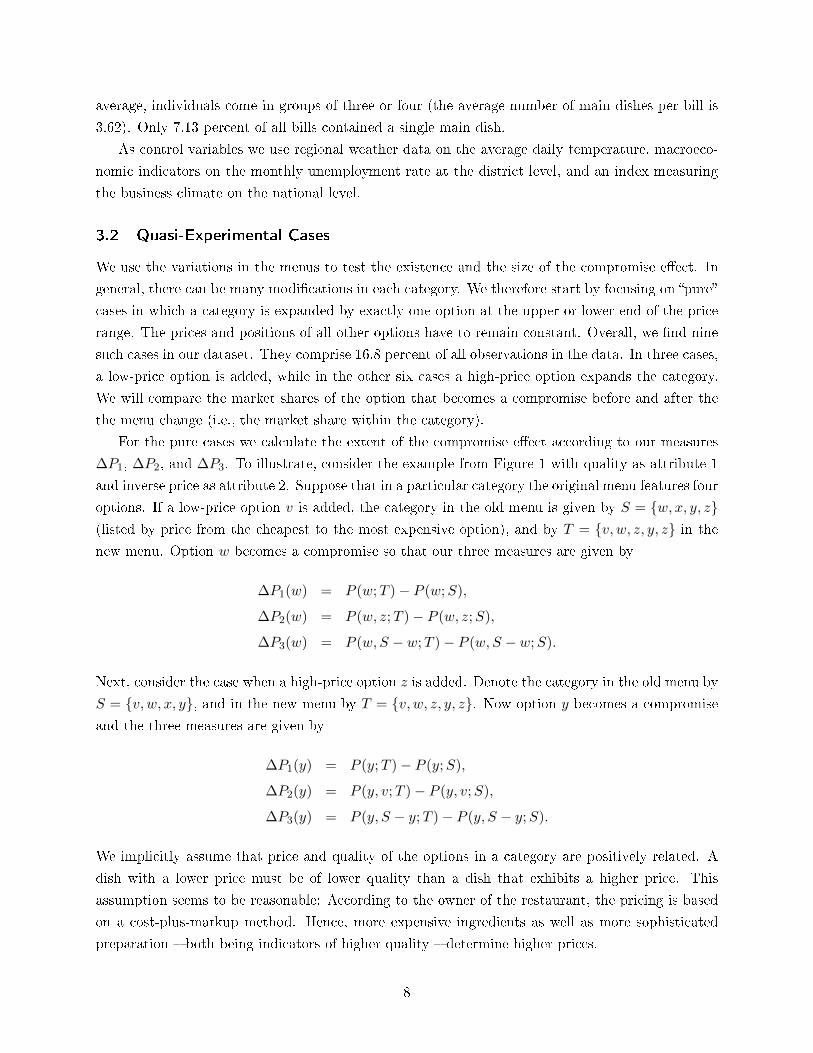
3.2 Quasi-Experimental Cases

We use the variations in the menus to test the existence and the size of the compromise e�ect. In

general, there can be many modi�cations in each category. We therefore start by focusing on �pure�

cases in which a category is expanded by exactly one option at the upper or lower end of the price

range. The prices and positions of all other options have to remain constant. Overall, we �nd nine

such cases in our dataset. They comprise 16.8 percent of all observations in the data. In three cases,

a low-price option is added, while in the other six cases a high-price option expands the category.

We will compare the market shares of the option that becomes a compromise before and after the

the menu change (i.e., the market share within the category).

For the pure cases we calculate the extent of the compromise e�ect according to our measures

∆P1, ∆P2, and ∆P3. To illustrate, consider the example from Figure 1 with quality as attribute 1

and inverse price as attribute 2. Suppose that in a particular category the original menu features four

options. If a low-price option v is added, the category in the old menu is given by S = {w, x, y, z}(listed by price from the cheapest to the most expensive option), and by T = {v, w, z, y, z} in the

new menu. Option w becomes a compromise so that our three measures are given by

∆P1(w) = P (w;T )− P (w;S),

∆P2(w) = P (w, z;T )− P (w, z;S),

∆P3(w) = P (w, S − w;T )− P (w, S − w;S).

Next, consider the case when a high-price option z is added. Denote the category in the old menu by

S = {v, w, x, y}, and in the new menu by T = {v, w, z, y, z}. Now option y becomes a compromise

and the three measures are given by

∆P1(y) = P (y;T )− P (y;S),

∆P2(y) = P (y, v;T )− P (y, v;S),

∆P3(y) = P (y, S − y;T )− P (y, S − y;S).

We implicitly assume that price and quality of the options in a category are positively related. A

dish with a lower price must be of lower quality than a dish that exhibits a higher price. This

assumption seems to be reasonable: According to the owner of the restaurant, the pricing is based

on a cost-plus-markup method. Hence, more expensive ingredients as well as more sophisticated

preparation � both being indicators of higher quality � determine higher prices.

8

3.3 Regression Analysis

In this subsection, we outline our empirical strategy. We �rst estimate discrete choice conditional

logit models. They allow us to control for alternative-speci�c and contextual factors which poten-

tially in�uence customers' decisions so that we can use the entire dataset. Next, we depart from

the IIA assumption and allow for correlated unobserved heterogeneity in a mixed logit framework.

Finally, we apply an instrumental variable (IV) framework to address potential endogeneity issues,

which may arise if the restaurant owner exploits the compromise e�ect.

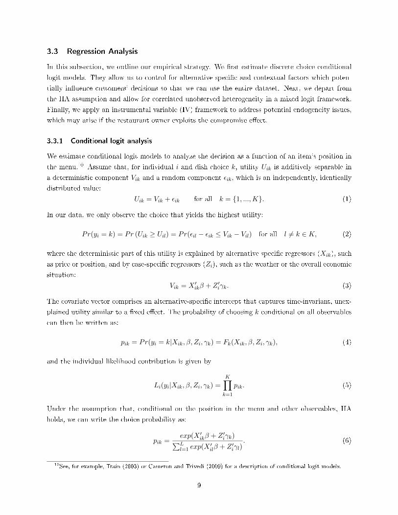
3.3.1 Conditional logit analysis

We estimate conditional logit models to analyze the decision as a function of an item's position in

the menu.10 Assume that, for individual i and dish choice k, utility Uik is additively separable in

a deterministic component Vik and a random component εik, which is an independently, identically

distributed value:

Uik = Vik + εik for all k = {1, ...,K}. (1)

In our data, we only observe the choice that yields the highest utility:

Pr(yi = k) = Pr (Uik ≥ Uil) = Pr(εil − εik ≤ Vik − Vil) for all l 6= k ∈ K, (2)

where the deterministic part of this utility is explained by alternative speci�c regressors (Xik), such

as price or position, and by case-speci�c regressors (Zi), such as the weather or the overall economic

situation:

Vik = X ′ikβ + Z ′iγk. (3)

The covariate vector comprises an alternative-speci�c intercept that captures time-invariant, unex-

plained utility similar to a �xed e�ect. The probability of choosing k conditional on all observables

can then be written as:

pik = Pr(yi = k|Xik, β, Zi, γk) = Fk(Xik, β, Zi, γk), (4)

and the individual likelihood contribution is given by

Li(yi|Xik, β, Zi, γk) =

K∏k=1

pik. (5)

Under the assumption that, conditional on the position in the menu and other observables, IIA

holds, we can write the choice probability as:

pik =exp(X ′ikβ + Z ′iγk)∑Ll=1 exp(X

′ilβ + Z ′iγl)

. (6)

10See, for example, Train (2003) or Cameron and Trivedi (2009) for a description of conditional logit models.

9

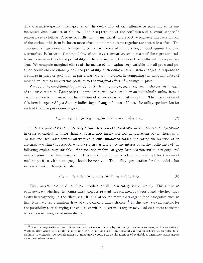
The alternative-speci�c intercepts re�ect the desirability of each alternative according to its un-

measured time-invariant attributes. The interpretation of the coe�cients of alternative-speci�c

regressors is as follows: A positive coe�cient means that if the respective regressor increases for one

of the options, this item is chosen more often and all other items together are chosen less often. The

case-speci�c regressors can be interpreted as parameters of a binary logit model against the base

alternative. Relative to the probability of the base alternative, an increase of the regressor leads

to an increase in the choice probability of the alternative if the respective coe�cient has a positive

sign. We compute marginal e�ects at the means of the explanatory variables for all price and po-

sition coe�cients to quantify how the probability of choosing a certain item changes in response to

a change in price or position. In particular, we are interested in comparing the marginal e�ect of

moving an item to an extreme position to the marginal e�ect of a change in price.

We apply the conditional logit model to (i) the nine pure cases, (ii) all menu choices within each

of the six categories. Using only the pure cases, we investigate how an individual's utility from a

certain choice is in�uenced by the addition of a new extreme-position option. The introduction of

this item is captured by a dummy indicating a change of menus. Hence, the utility speci�cation for

each of the nine pure cases is given by

Uik = β0 + β1 priceik + γ1kmenu changei + Z ′iγk + εik. (7)

Since the pure cases comprise only a small fraction of the dataset, we run additional regressions

in order to exploit all menu changes, even if they imply multiple modi�cations of the choice sets.

To this end, we coded several alternative-speci�c dummy variables, indicating the location of an

alternative within the respective category. In particular, we are interested in the coe�cients of the

following explanatory variables: �rst position within category, last position within category, and

median position within category. If there is a compromise e�ect, all signs except for the one of

median position within category should be negative. The utility speci�cation for the models that

exploit all menu changes equals

Uik = β0 + β1 priceik + β2 positionik + Z ′iγk + εik. (8)

First, we estimate conditional logit models for all menu categories separately. This allows us

to investigate whether the compromise e�ect is present in each menu category, and whether there

exists heterogeneity in the e�ect, e.g., if it is larger for more extravagant food categories such as

�sh. Next, we use a random draw of the complete menu choices.11 In this way, we can control for

the possibility that changing the choice set within a certain category may lead customers to switch

to a di�erent category of main dishes.

11Due to computational restrictions, we reduce the sample size by randomly drawing a subsample of observations.With 75 alternatives in the full menu sample, the simulations are computationally infeasible otherwise. In both steps,we have to estimate the models using an unbalanced choice set, as the number of available alternatives varies acrossindividual observations.

10

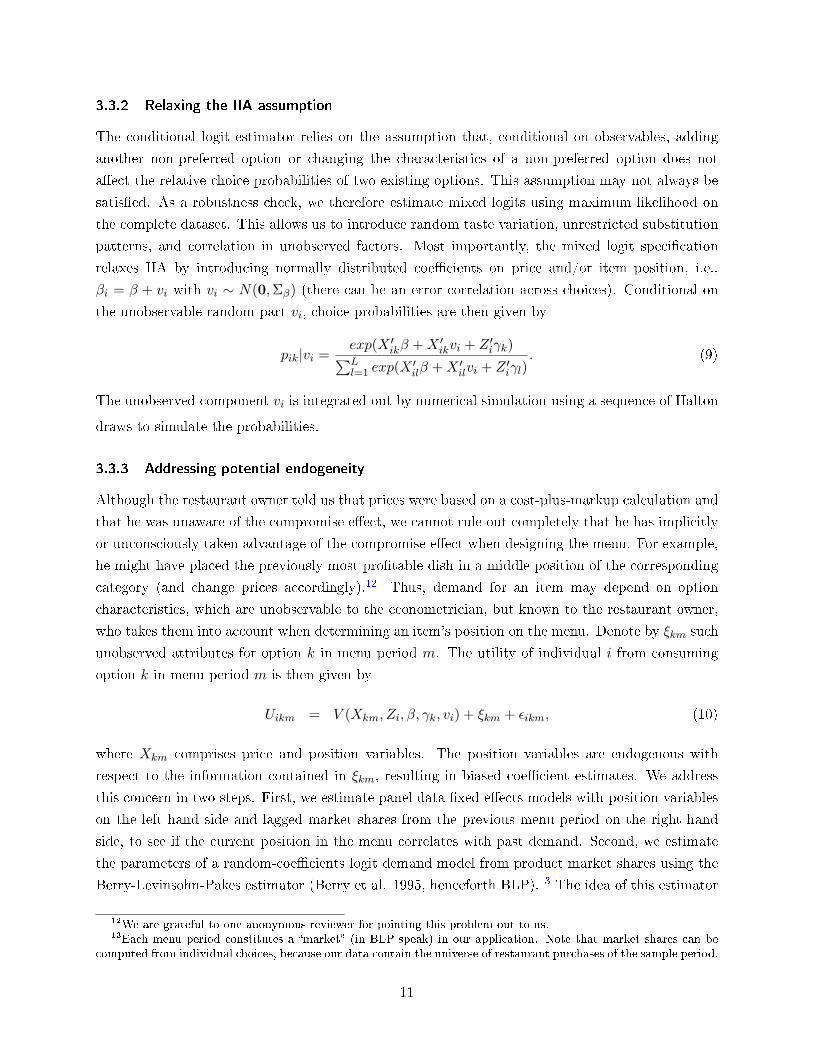
3.3.2 Relaxing the IIA assumption

The conditional logit estimator relies on the assumption that, conditional on observables, adding

another non-preferred option or changing the characteristics of a non-preferred option does not

a�ect the relative choice probabilities of two existing options. This assumption may not always be

satis�ed. As a robustness check, we therefore estimate mixed logits using maximum likelihood on

the complete dataset. This allows us to introduce random taste variation, unrestricted substitution

patterns, and correlation in unobserved factors. Most importantly, the mixed logit speci�cation

relaxes IIA by introducing normally distributed coe�cients on price and/or item position, i.e.,

βi = β + vi with vi ∼ N(0,Σβ) (there can be an error correlation across choices). Conditional on

the unobservable random part vi, choice probabilities are then given by

pik|vi =exp(X ′ikβ +X ′ikvi + Z ′iγk)∑Ll=1 exp(X

′ilβ +X ′ilvi + Z ′iγl)

. (9)

The unobserved component vi is integrated out by numerical simulation using a sequence of Halton

draws to simulate the probabilities.

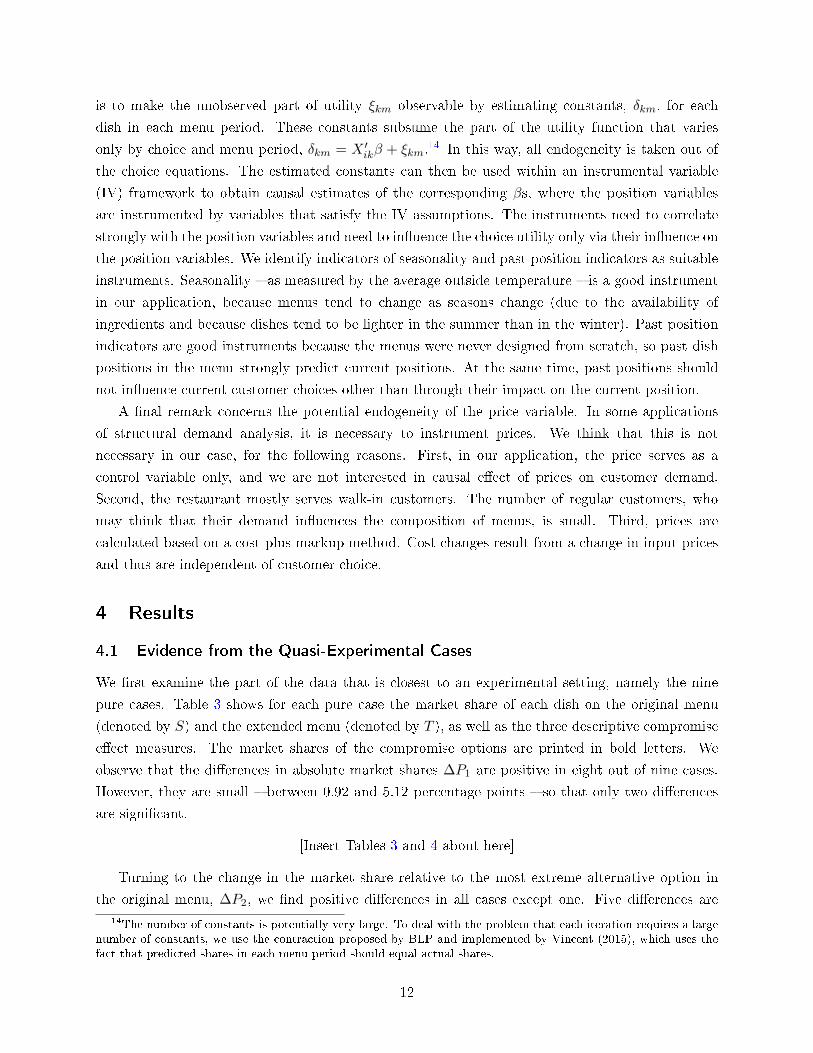
3.3.3 Addressing potential endogeneity

Although the restaurant owner told us that prices were based on a cost-plus-markup calculation and

that he was unaware of the compromise e�ect, we cannot rule out completely that he has implicitly

or unconsciously taken advantage of the compromise e�ect when designing the menu. For example,

he might have placed the previously most pro�table dish in a middle position of the corresponding

category (and change prices accordingly).12 Thus, demand for an item may depend on option

characteristics, which are unobservable to the econometrician, but known to the restaurant owner,

who takes them into account when determining an item's position on the menu. Denote by ξkm such

unobserved attributes for option k in menu period m. The utility of individual i from consuming

option k in menu period m is then given by

Uikm = V (Xkm, Zi, β, γk, vi) + ξkm + εikm, (10)

where Xkm comprises price and position variables. The position variables are endogenous with

respect to the information contained in ξkm, resulting in biased coe�cient estimates. We address

this concern in two steps. First, we estimate panel data �xed e�ects models with position variables

on the left hand side and lagged market shares from the previous menu period on the right hand

side, to see if the current position in the menu correlates with past demand. Second, we estimate

the parameters of a random-coe�cients logit demand model from product market shares using the

Berry-Levinsohn-Pakes estimator (Berry et al. 1995, henceforth BLP).13 The idea of this estimator

12We are grateful to one anonymous reviewer for pointing this problem out to us.13Each menu period constitutes a �market� (in BLP-speak) in our application. Note that market shares can be

computed from individual choices, because our data contain the universe of restaurant purchases of the sample period.

11

is to make the unobserved part of utility ξkm observable by estimating constants, δkm, for each

dish in each menu period. These constants subsume the part of the utility function that varies

only by choice and menu period, δkm = X ′ikβ + ξkm.14 In this way, all endogeneity is taken out of

the choice equations. The estimated constants can then be used within an instrumental variable

(IV) framework to obtain causal estimates of the corresponding βs, where the position variables

are instrumented by variables that satisfy the IV assumptions. The instruments need to correlate

strongly with the position variables and need to in�uence the choice utility only via their in�uence on

the position variables. We identify indicators of seasonality and past position indicators as suitable

instruments. Seasonality � as measured by the average outside temperature � is a good instrument

in our application, because menus tend to change as seasons change (due to the availability of

ingredients and because dishes tend to be lighter in the summer than in the winter). Past position

indicators are good instruments because the menus were never designed from scratch, so past dish

positions in the menu strongly predict current positions. At the same time, past positions should

not in�uence current customer choices other than through their impact on the current position.

A �nal remark concerns the potential endogeneity of the price variable. In some applications

of structural demand analysis, it is necessary to instrument prices. We think that this is not

necessary in our case, for the following reasons. First, in our application, the price serves as a

control variable only, and we are not interested in causal e�ect of prices on customer demand.

Second, the restaurant mostly serves walk-in customers. The number of regular customers, who

may think that their demand in�uences the composition of menus, is small. Third, prices are

calculated based on a cost-plus-markup method. Cost changes result from a change in input prices

and thus are independent of customer choice.

4 Results

4.1 Evidence from the Quasi-Experimental Cases

We �rst examine the part of the data that is closest to an experimental setting, namely the nine

pure cases. Table 3 shows for each pure case the market share of each dish on the original menu

(denoted by S) and the extended menu (denoted by T ), as well as the three descriptive compromise

e�ect measures. The market shares of the compromise options are printed in bold letters. We

observe that the di�erences in absolute market shares ∆P1 are positive in eight out of nine cases.

However, they are small � between 0.92 and 5.12 percentage points � so that only two di�erences

are signi�cant.

[Insert Tables 3 and 4 about here]

Turning to the change in the market share relative to the most extreme alternative option in

the original menu, ∆P2, we �nd positive di�erences in all cases except one. Five di�erences are

14The number of constants is potentially very large. To deal with the problem that each iteration requires a largenumber of constants, we use the contraction proposed by BLP and implemented by Vincent (2015), which uses thefact that predicted shares in each menu period should equal actual shares.

12

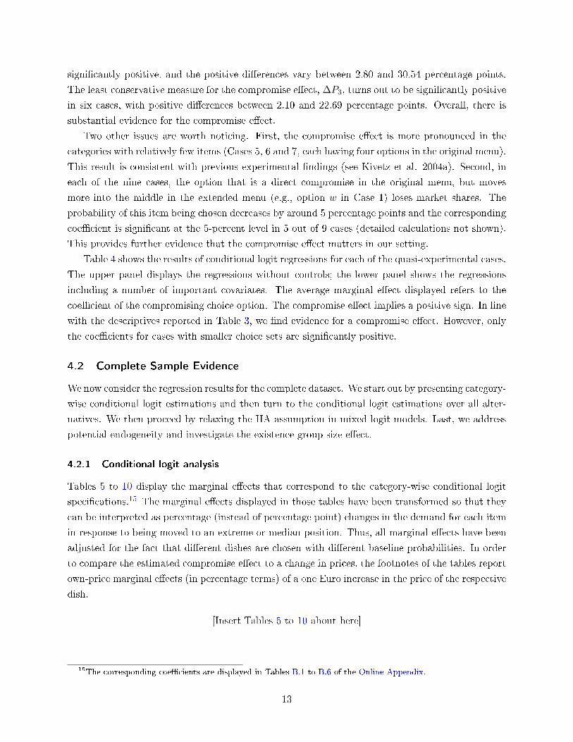
signi�cantly positive, and the positive di�erences vary between 2.80 and 30.54 percentage points.

The least conservative measure for the compromise e�ect, ∆P3, turns out to be signi�cantly positive

in six cases, with positive di�erences between 2.10 and 22.69 percentage points. Overall, there is

substantial evidence for the compromise e�ect.

Two other issues are worth noticing. First, the compromise e�ect is more pronounced in the

categories with relatively few items (Cases 5, 6 and 7, each having four options in the original menu).

This result is consistent with previous experimental �ndings (see Kivetz et al. 2004a). Second, in

each of the nine cases, the option that is a direct compromise in the original menu, but moves

more into the middle in the extended menu (e.g., option w in Case 1) loses market shares. The

probability of this item being chosen decreases by around 5 percentage points and the corresponding

coe�cient is signi�cant at the 5-percent level in 5 out of 9 cases (detailed calculations not shown).

This provides further evidence that the compromise e�ect matters in our setting.

Table 4 shows the results of conditional logit regressions for each of the quasi-experimental cases.

The upper panel displays the regressions without controls; the lower panel shows the regressions

including a number of important covariates. The average marginal e�ect displayed refers to the

coe�cient of the compromising choice option. The compromise e�ect implies a positive sign. In line

with the descriptives reported in Table 3, we �nd evidence for a compromise e�ect. However, only

the coe�cients for cases with smaller choice sets are signi�cantly positive.

4.2 Complete Sample Evidence

We now consider the regression results for the complete dataset. We start out by presenting category-

wise conditional logit estimations and then turn to the conditional logit estimations over all alter-

natives. We then proceed by relaxing the IIA assumption in mixed logit models. Last, we address

potential endogeneity and investigate the existence group size e�ect.

4.2.1 Conditional logit analysis

Tables 5 to 10 display the marginal e�ects that correspond to the category-wise conditional logit

speci�cations.15 The marginal e�ects displayed in those tables have been transformed so that they

can be interpreted as percentage (instead of percentage point) changes in the demand for each item

in response to being moved to an extreme or median position. Thus, all marginal e�ects have been

adjusted for the fact that di�erent dishes are chosen with di�erent baseline probabilities. In order

to compare the estimated compromise e�ect to a change in prices, the footnotes of the tables report

own-price marginal e�ects (in percentage terms) of a one Euro increase in the price of the respective

dish.

[Insert Tables 5 to 10 about here]

15The corresponding coe�cients are displayed in Tables B.1 to B.6 of the Online Appendix.

13


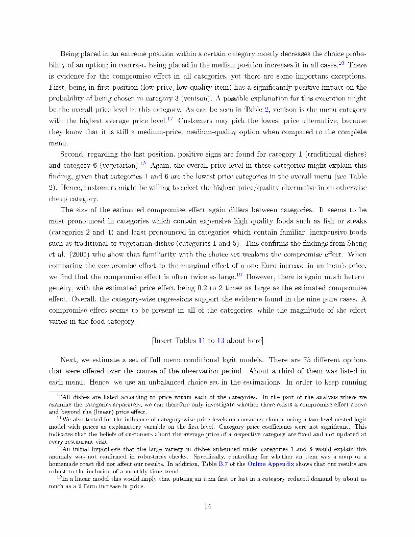
Being placed in an extreme position within a certain category mostly decreases the choice proba-

bility of an option; in contrast, being placed in the median position increases it in all cases.16 There

is evidence for the compromise e�ect in all categories, yet there are some important exceptions.

First, being in �rst position (low-price, low-quality item) has a signi�cantly positive impact on the

probability of being chosen in category 3 (venison). A possible explanation for this exception might

be the overall price level in this category. As can be seen in Table 2, venison is the menu category

with the highest average price level.17 Customers may pick the lowest price alternative, because

they know that it is still a medium-price, medium-quality option when compared to the complete

menu.

Second, regarding the last position, positive signs are found for category 1 (traditional dishes)

and category 6 (vegetarian).18 Again, the overall price level in these categories might explain this

�nding, given that categories 1 and 6 are the lowest price categories in the overall menu (see Table

2). Hence, customers might be willing to select the highest price/quality alternative in an otherwise

cheap category.

The size of the estimated compromise e�ect again di�ers between categories. It seems to be

most pronounced in categories which contain expensive high quality foods such as �sh or steaks

(categories 2 and 4) and least pronounced in categories which contain familiar, inexpensive foods

such as traditional or vegetarian dishes (categories 1 and 5). This con�rms the �ndings from Sheng

et al. (2005) who show that familiarity with the choice set weakens the compromise e�ect. When

comparing the compromise e�ect to the marginal e�ect of a one Euro increase in an item's price,

we �nd that the compromise e�ect is often twice as large.19 However, there is again much hetero-

geneity, with the estimated price e�ect being 0.2 to 2 times as large as the estimated compromise

e�ect. Overall, the category-wise regressions support the evidence found in the nine pure cases. A

compromise e�ect seems to be present in all of the categories, while the magnitude of the e�ect

varies in the food category.


Next, we estimate a set of full menu conditional logit models. There are 75 di�erent options

that were o�ered over the course of the observation period. About a third of them was listed in

each menu. Hence, we use an unbalanced choice set in the estimations. In order to keep running

16All dishes are listed according to price within each of the categories. In the part of the analysis where weexamine the categories separately, we can therefore only investigate whether there exists a compromise e�ect aboveand beyond the (linear) price e�ect.

17We also tested for the in�uence of category-wise price levels on consumer choices using a two-level nested logitmodel with prices as explanatory variable on the �rst-level. Category price coe�cients were not signi�cant. Thisindicates that the beliefs of customers about the average price of a respective category are �xed and not updated atevery restaurant visit.

18An initial hypothesis that the large variety in dishes subsumed under categories 1 and 6 would explain thisanomaly was not con�rmed in robustness checks. Speci�cally, controlling for whether an item was a soup or ahomemade roast did not a�ect our results. In addition, Table B.7 of the Online Appendix shows that our results arerobust to the inclusion of a monthly time trend.

19In a linear model this would imply that putting an item �rst or last in a category reduced demand by about asmuch as a 2 Euro increase in price.

14


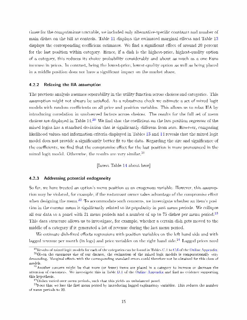
times for the computations tractable, we included only alternative-speci�c constants and number of

main dishes on the bill as controls. Table 11 displays the estimated marginal e�ects and Table 13

displays the corresponding coe�cient estimates. We �nd a signi�cant e�ect of around 20 percent

for the last position within category. Hence, if a dish is the highest-price, highest-quality option

of a category, this reduces its choice probability considerably and about as much as a one Euro

increase in prices. In contrast, being the lowest-price, lowest-quality option as well as being placed

in a middle position does not have a signi�cant impact on the market share.

4.2.2 Relaxing the IIA assumption

The previous analysis assumes separability in the utility function across choices and categories. This

assumption might not always be satis�ed. As a robustness check we estimate a set of mixed logit

models with random coe�cients on all price and position variables. This allows us to relax IIA by

introducing correlation in unobserved factors across choices. The results for the full set of menu

choices are displayed in Table 14.20 We �nd that the coe�cient on the last position regressor of the

mixed logits has a standard deviation that is signi�cantly di�erent from zero. However, comparing

likelihood values and information criteria displayed in Tables 13 and 14 reveals that the mixed logit

model does not provide a signi�cantly better �t to the data. Regarding the size and signi�cance of

the coe�cients, we �nd that the compromise e�ect for the last position is more pronounced in the

mixed logit model. Otherwise, the results are very similar.21

[Insert Table 14 about here]

4.2.3 Addressing potential endogeneity

So far, we have treated an option's menu position as an exogenous variable. However, this assump-

tion may be violated, for example, if the restaurant owner takes advantage of the compromise e�ect

when designing the menu.22 To accommodate such concerns, we investigate whether an item's posi-

tion in the current menu is signi�cantly related to its popularity in past menu periods. We collapse

all our data to a panel with 21 menu periods and a number of up to 75 dishes per menu period.23

This data structure allows us to investigate, for example, whether a certain dish gets moved to the

middle of a category if it generated a lot of revenue during the last menu period.

We estimate dish-�xed e�ects regressions with position variables on the left hand side and with

lagged revenue per month (in logs) and price variables on the right hand side.24 Lagged prices need

20Results of mixed logit models for each of the categories can be found in Tables C.1 to C.6 of the Online Appendix.21Given the enormous size of our dataset, the estimation of the mixed logit models is computationally very

demanding. Marginal e�ects with the corresponding standard errors could therefore not be obtained for this class ofmodels.

22Another concern might be that more (or fewer) items are placed in a category to increase or decrease theattention of customers. We investigate this in Table D.1 of the Online Appendix and �nd no evidence supportingthis hypothesis.

23Dishes varied over menu periods, such that this yields an unbalanced panel.24Note that we lose the �rst menu period by introducing lagged explanatory variables. This reduces the number

of menu periods to 20.

15



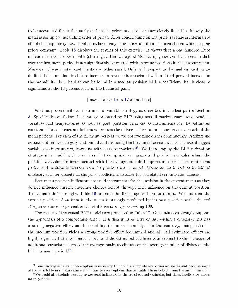
to be accounted for in this analysis, because prices and positions are closely linked in the way the

menu is set up (by ascending order of price). After conditioning on the price, revenue is informative

of a dish's popularity, i.e., it indicates how many times a certain item has been chosen while keeping

prices constant. Table 15 displays the results of this exercise. It shows that a one hundred Euro

increase in revenue per month (starting at the average of 385 Euro) generated by a certain dish

over the last menu period is not signi�cantly correlated with extreme positions in the current menu.

Moreover, the estimated coe�cients are rather small. Only with respect to the median position we

do �nd that a one hundred Euro increase in revenue is associated with a 2 to 4 percent increase in

the probability that the dish can be found in a median position with a coe�cient that is close to

signi�cant at the 10-percent level in the balanced panel.


We thus proceed with an instrumental variable strategy as described in the last part of Section

3. Speci�cally, we follow the strategy proposed by BLP using overall market shares as dependent

variables and temperatures as well as past position variables as instruments for the estimated

constants. To construct market shares, we use the universe of restaurant purchases over each of the

menu periods. For each of the 21 menu periods m, we observe nine dishes continuously. Adding one

outside option per category and period and dropping the �rst menu period, due to the use of lagged

variables as instruments, leaves us with 300 observations.25 We then employ the BLP estimation

strategy in a model with covariates that comprise item prices and position variables where the

position variables are instrumented with the average outside temperature over the current menu

period and position indicators from the previous menu period. Moreover, we introduce individual

unobserved heterogeneity in the price coe�cients to allow for correlated errors across choices.

Past menu position indicators are valid instruments for the position in the current menu as they

do not in�uence current customer choices except through their in�uence on the current position.

To evaluate their strength, Table 16 presents the �rst stage estimation results. We �nd that the

current position of an item in the menu is strongly predicted by its past position with adjusted

R-squares above 60 percent and F-statistics strongly exceeding 100.

The results of the causal BLP models are presented in Table 17. Our estimates strongly support

the hypothesis of a compromise e�ect. If a dish is listed �rst or last within a category, this has

a strong negative e�ect on choice utility (columns 1 and 2). On the contrary, being listed at

the medium position yields a strong positive e�ect (columns 3 and 4). All estimated e�ects are

highly signi�cant at the 1-percent level and the estimated coe�cients are robust to the inclusion of

additional covariates such as the average business climate or the average number of dishes on the

bill in a menu period.26

25Constructing such an outside option is necessary to obtain a complete set of market shares and because muchof the variability in the data stems from exactly those options that are added to or deleted from the menu over time.

26We could also include evening or weekend indicators in the set of control variables, but those hardly vary acrossmenu periods.

16

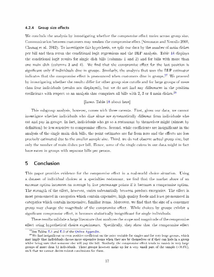
4.2.4 Group size e�ects

We conclude the analysis by investigating whether the compromise e�ect varies across group size.

Communication between customers may weaken the compromise e�ect (Simonson and Nowalis 2000,

Chuang et al. 2012). To investigate this hypothesis, we split our data by the number of main dishes

per bill and then rerun the conditional logit regressions and the BLP analysis. Table 18 displays

the conditional logit results for single dish bills (columns 1 and 2) and for bills with more than

one main dish (columns 3 and 4). We �nd that the compromise e�ect for the last position is

signi�cant only if individuals dine in groups. Similarly, the analysis that uses the BLP estimator

indicates that the compromise e�ect is pronounced when customers dine in groups.27 We proceed

by investigating whether the results di�er for other group size cuto�s and for large groups of more

than four individuals (results not displayed), but we do not �nd any di�erences in the position

coe�cients with respect to an analysis that comprises all bills with 2, 3 or 4 main dishes.28

[Insert Table 18 about here]

This subgroup analysis, however, comes with three caveats. First, given our data, we cannot

investigate whether individuals who dine alone are systematically di�erent from individuals who

eat and pay in groups. In fact, individuals who go to a restaurant by themselves might (almost by

de�nition) be less sensitive to compromise e�ects. Second, while coe�cients are insigni�cant in the

analysis of the single main dish bills, the point estimates are far from zero and the e�ects are less

precisely estimated due to the smaller sample size. Third, we do not observe actual group size, but

only the number of main dishes per bill. Hence, some of the single eaters in our data might in fact

have eaten in groups with separate bills per person.

5 Conclusion

This paper provides evidence for the compromise e�ect in a real-world choice situation. Using

a dataset of individual choices at a specialties restaurant, we �nd that the market share of an

extreme option increases on average by �ve percentage points if it becomes a compromise option.

The strength of the e�ect, however, varies substantially between product categories. The e�ect is

most pronounced in categories which contain expensive, high quality foods and least pronounced in

categories which contain inexpensive, familiar items. Moreover, we �nd that the size of a consumer

group may change the magnitude of the compromise e�ect. While choices by groups exhibit a

signi�cant compromise e�ect, it becomes statistically insigni�cant for single individuals.

These results validate a large literature that analyzes the scope and magnitude of the compromise

e�ect using hypothetical choice experiments. Speci�cally, they show that the compromise e�ect

27See Tables E.1 and E.2 of the Online Appendix.28We �nd insigni�cant or even positive coe�cient on the price variable for singles and for very large groups, which

may imply that individuals choose more expensive items when they are by themselves or if they can hide in a groupwhilst being sure that someone else will pay the bill. Similarly, the compromise e�ect tends to vanish in very largegroups of more than 12 individuals. These groups however make up for a very small part of the sample (<0.3%),such that we cannot derive robust conclusions for them.

17


may arise in environments that exhibit many features which potentially reduce the strength of

the compromise e�ect, i.e., a large choice set, decision makers who are familiar with the choice

situation and (most likely) also with some options from the choice set, as well as the opportunity

of communication between customers to discuss or recommend choices.

Practitioners and marketers can take advantage of these results by appropriately designing choice

menus. This seems to be especially relevant for menus in which a large set of options is organized

in several sub-categories (as is common in restaurants) and consumers have to weigh alternatives

with respect to several attributes. There are plenty of examples outside of gastronomy where this

is the case, e.g., internet commerce, trade of complex goods (such as cars) with many optional add-

ons, voting in political elections, or Likert scales in surveys. In particular, the availability of large

datasets on consumer choices will allow �rms to �ne-tune their strategies to exploit the compromise

e�ect in the future.

18

References

Abeler, J., Marklein, F., forthcoming. Fungibility, Labels, and Consumption. Journal of the Euro-

pean Economic Association.

Apesteguia, J., Ballester, M., 2013. Choice by sequential procedures. Games and Economic Behavior

77(1), 90�99.

Berry, S., Levinsohn, J., Pakes, A., 1995. Automobile prices in market equilibrium. Econometrica

63(4), 841�890.

Cameron, A. C., Trivedi, P. K., 2009. Microeconomics Using Stata. Stata Press.

Chuang, S.-C., Cheng, Y.-H., Hsu, C.-T., 2012. The in�uence of suggestions of reference groups in

the compromise e�ect. Journal of Economic Psychology 33(3), 554�565.

De Clippel, G., Eliaz, K., 2012. Reason-based Choice: A Bargaining Rationale for the Attraction

and Compromise E�ects. Theoretical Economics 7(1), 125�162.

Dhar, R., Nowlis, S. M., Sherman, S. J., 2000. Trying hard or hardly trying: An analysis of context

e�ects in choice. Journal of Consumer Psychology 9(4), 189�200.

Dhar, R., Simonson, I., 2003. The E�ect of Forced Choice on Choice. Journal of Marketing Research

40(2), 146�160.

DellaVigna, S., 2009. Psychology and Economics: Evidence from the Field. Journal of Economic

Literature 47(2), 315�372.

DellaVigna, S., Malmendier, U., 2006. Paying Not to Go to the Gym. American Economic Review

96(3), 694�719.

Doyle, J. R., O'Connor, D. J., Reynolds, G. M., Bottomley, P. A., 1999. The robustness of the

asymmetrically dominated e�ect: Buying frames, phantom alternatives, and in-store purchases.

Psychology and Marketing 16(3), 225�243.

Ehlers, L., Sprumont, Y., 2008. Weakened WARP and top-cycle choice rules. Journal of Mathemat-

ical Economics 44(1), 87�94.

Iyengar, S. S., Lepper, M. R., 2000. When choice is demotivating: Can one desire too much of a

good thing? Journal of Personality and Social Psychology 79(6), 995�1006.

Kamenica, E., 2008. Contextual Inference in Markets: On the Informational Content of Product

Lines. American Economic Review 98(5), 2127�2149.

Kivetz, R., Netzer, O., Srinivasan, V., 2004a. Alternative models for capturing the compromise

e�ect. Journal of Marketing Research 41(3), 237�257.

19

Kivetz, R., Netzer, O., Srinivasan, V., 2004b. Extending compromise e�ect models to complex

buying situations and other context e�ects. Journal of Marketing Research 41(3), 262�268.

Levitt, S., List, J. A., 2007. Viewpoint: On the generalizability of lab behaviour to the �eld.

Canadian Journal of Economics 40(2), 347�370.

List, J., Rasul, I., 2010. Field Experiments in Labor Economics. In D. Card and O. Ashenfelter

(eds): Handbook of Labor Economics (Vol. 4a), Amsterdam, North Holland.

Lombardi, M., 2008. Uncovered set choice rules. Social Choice and Welfare 31(2), 271�279.

Manzini, P., Mariotti, M., 2007. Sequentially Rationalizable Choice. American Economic Review

97(5), 1824�1839.

Masatlioglu, Y., Ok, E., 2005. Rational choice with status quo bias. Journal of Economic Theory

121(1), 1�29.

Prelec, D., Wernerfelt, B., Zettelmeyer, F., 1997. The Role of Inference in Context E�ects: Inferring

What You Want from What is Available. Journal of Consumer Research 24(1), 118�125.

Rubinstein, A., Salant, Y., 2006. A model of choice from lists. Theoretical Economics 1(1), 3�17.

Salant, Y., Rubinstein, A., 2008. (A, f): Choice with Frames. Review of Economic Studies 75(4),

1287�1296.

Sheng, S., Parker, A. M., Nakamoto, K., 2005. Understanding the mechanism and determinants of

compromise e�ects. Psychology and Marketing 22(7), 591�609.

Simonson, I., 1989. Choice Based on Reasons: The Case of Attraction and Compromise E�ects.

Journal of Consumer Research 16(2), 158�174.

Simonson, I., Tversky, A., 1992. Choice in Context: Tradeo� Contrast and Extremeness Aversion.

Journal of Marketing Research 29(3), 281�295.

Simonson, I., Nowlis, S. M., 2000. The role of explanations and need for uniqueness in consumer

decision making: Unconventional choices based on reasons. Journal of Consumer Research 27(1),

49�68.

Train, K., 2003. Discrete choice methods with simulation. Cambridge University Press, New York.

Tversky, A., Simonson, I., 1993. Context-Dependent Preferences. Management Science 39(10), 1179�

1189.

Vincent, D. W., 2015. The Berry-Levinsohn-Pakes estimator of the random-coe�cients logit demand

model. Stata Journal 15(3), 854�880.

Wernerfelt, B., 1995. A rational reconstruction of the compromise e�ect: Using market data to infer

utilities. Journal of Consumer Research 21(4), 627�633.

20

Tables

Table 1: Summary statistics of the main explanatory variables

Variable Mean Std. Dev. Min. Max.

price of item in EUR (per unit) 10.05 2.63 3.5 17.8number of dishes in category 4.92 1.44 2 8�rst position within category 0.23 0.42 0 1last position within category 0.22 0.42 0 1median position within category 0.38 0.49 0 1number of main dishes on the bill 3.62 2.24 1 15outside table 0.29 0.46 0 1monthly business climate 96.69 7.04 82.3 108.9evening order 0.28 0.45 0 1public holiday 0.05 0.22 0 1weekend 0.57 0.49 0 1

N 88113

Notes: The table displays means and standard deviations of the main explanatory variables. Outside table indicates whethera table is located in the outside area of the restaurant. Monthly business climate refers to the CESifo monthly business cycleindicator. Evening order indicates whether a dish was ordered after 5pm. Public holiday indicates whether a dish was orderedon a public holiday. Weekend indicates whether a dish was ordered on a weekend.

Table 2: Summary statistics by category

random shares price �rst position last position median position

N All Median Mean StdDev Mean StdDev Mean StdDev Mean StdDev

traditional 24,689 0.15 0.22 8.85 2.01 0.14 0.35 0.31 0.46 0.25 0.43�sh 13,568 0.21 0.31 11.07 1.64 0.19 0.40 0.18 0.38 0.37 0.48venison 13,763 0.24 0.43 12.95 1.82 0.25 0.43 0.16 0.37 0.54 0.50steak 19,402 0.21 0.35 10.75 1.58 0.23 0.42 0.19 0.39 0.44 0.50poultry 7,436 0.29 0.42 9.51 2.34 0.32 0.47 0.26 0.44 0.50 0.50vegetarian 9,255 0.22 0.33 6.36 2.00 0.42 0.49 0.17 0.38 0.28 0.45

Notes: The table displays means and standard deviations of the position variables by category. Random share (All) refers tothe share of dishes that would have been ordered at random, as de�ned by one divided by the average total number of dishesper category. Random share (Median) refers to the share of median dishes that would have been ordered if preferences wererandom. The middle position is de�ned such that it equals the median whenever there is an unequal number of items. Whenthere is an equal number of items within a category, the two middle items are both de�ned to be at the median position withinthe category.

21

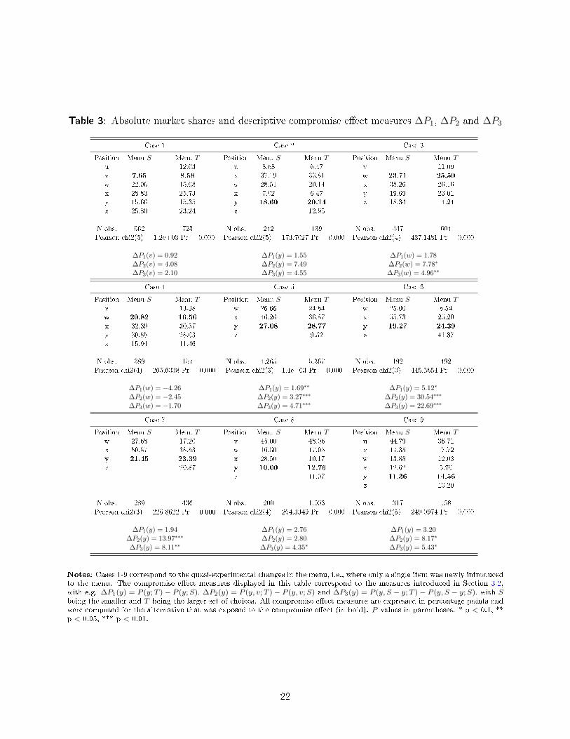
Table 3: Absolute market shares and descriptive compromise e�ect measures ∆P1, ∆P2 and ∆P3

Case 1 Case 2 Case 3

Position Menu S Menu T Position Menu S Menu T Position Menu S Menu Tu 12.03 u 8.68 6.47 v 11.09v 7.65 8.58 v 37.19 33.81 w 23.71 25.50

w 22.06 15.08 w 28.51 20.14 x 38.26 26.16x 28.83 25.73 x 7.02 6.47 y 19.69 23.01y 15.66 15.35 y 18.60 20.14 z 18.34 14.24z 25.80 23.24 z 12.95

N obs. 562 723 N obs. 242 139 N obs. 447 604Pearson chi2(5) = 1.2e+03 Pr = 0.000 Pearson chi2(5) = 173.7027 Pr = 0.000 Pearson chi2(4) = 437.1481 Pr = 0.000

∆P1(v) = 0.92 ∆P1(y) = 1.55 ∆P1(w) = 1.78∆P2(v) = 4.08 ∆P2(y) = 7.49 ∆P2(w) = 7.78∗

∆P3(v) = 2.10 ∆P3(y) = 4.55 ∆P3(w) = 4.96∗∗


Position Menu S Menu T Position Menu S Menu T Position Menu S Menu Tv 13.38 w 26.66 24.84 w 25.00 8.54w 20.82 16.56 x 46.26 36.87 x 55.73 25.20x 32.39 30.57 y 27.08 28.77 y 19.27 24.39

y 30.85 28.03 z 9.52 z 41.87z 15.94 11.46

N obs. 389 157 N obs. 4,265 5,367 N obs. 192 492Pearson chi2(4) = 265.6338 Pr = 0.000 Pearson chi2(3) =1.4e+03 Pr = 0.000 Pearson chi2(3) = 445.5654 Pr = 0.000

∆P1(w) = −4.26 ∆P1(y) = 1.69∗∗ ∆P1(y) = 5.12∗

∆P2(w) = −2.45 ∆P2(y) = 3.27∗∗∗ ∆P2(y) = 30.54∗∗∗

∆P3(w) = −1.70 ∆P3(y) = 4.71∗∗∗ ∆P3(y) = 22.69∗∗∗


Position Menu S Menu T Position Menu S Menu T Position Menu S Menu Tw 27.68 17.20 v 45.00 48.06 u 44.79 36.71x 50.87 38.53 w 16.50 17.95 v 17.35 17.72y 21.45 23.39 x 28.50 10.17 w 13.88 12.03z 20.87 y 10.00 12.76 x 12.62 5.70

z 11.07 y 11.36 14.56

z 13.29

N obs. 289 436 N obs. 200 1,003 N obs. 317 158Pearson chi2(3) = 226.8622 Pr = 0.000 Pearson chi2(4) = 264.3349 Pr = 0.000 Pearson chi2(5) = 249.0974 Pr = 0.000

∆P1(y) = 1.94 ∆P1(y) = 2.76 ∆P1(y) = 3.20∆P2(y) = 13.97∗∗∗ ∆P2(y) = 2.80 ∆P2(y) = 8.17∗

∆P3(y) = 8.11∗∗ ∆P3(y) = 4.35∗ ∆P3(y) = 5.43∗

Notes: Cases 1-9 correspond to the quasi-experimental changes in the menu, i.e., where only a single item was newly introducedto the menu. The compromise e�ect measures displayed in this table correspond to the measures introduced in Section 3.2,with e.g. ∆P1(y) = P (y;T )− P (y;S), ∆P2(y) = P (y, v;T )− P (y, v;S) and ∆P3(y) = P (y, S − y;T )− P (y, S − y;S), with Sbeing the smaller and T being the larger set of choices. All compromise e�ect measures are expressed in percentage points andwere computed for the alternative that was exposed to the compromise e�ect (in bold). P -values in parentheses. * p < 0.1, **p < 0.05, *** p < 0.01.

22

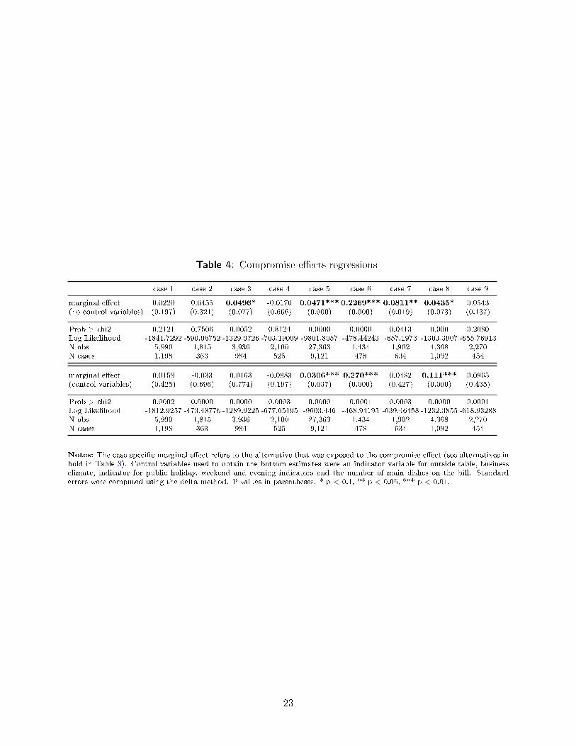
Table 4: Compromise e�ects regressions

case 1 case 2 case 3 case 4 case 5 case 6 case 7 case 8 case 9

marginal e�ect 0.0220 0.0455 0.0496* -0.0170 0.0471*** 0.2269*** 0.0811** 0.0435* 0.0543(no control variables) (0.197) (0.321) (0.077) (0.666) (0.000) (0.000) (0.019) (0.073) (0.137)

Prob > chi2 0.2121 0.7506 0.0052 0.8124 0.0000 0.0000 0.0413 0.000 0.2080Log Likelihood -1841.7292 -590.96752 -1329.9726 -703.19099 -9801.8057 -478.44243 -657.1973 -1303.3907 -655.76913N obs 5,990 1,815 3,936 2,100 27,363 1,434 1,902 4,368 2,270N cases 1,198 363 984 525 9,121 478 634 1,092 454

marginal e�ect 0.0159 -0.033 0.0163 -0.0883 0.0306*** 0.270*** 0.0482 0.111*** 0.0965(control variables) (0.425) (0.696) (0.774) (0.197) (0.037) (0.000) (0.427) (0.000) (0.435)

Prob > chi2 0.0002 0.0000 0.0000 0.0003 0.0000 0.0001 0.0003 0.0000 0.0001Log Likelihood -1812.9257 -473.48776 -1289.9225 -677.65195 -9603.446 -468.94195 -639.46458 -1232.3855 -618.93288N obs 5,990 1,815 3,936 2,100 27,363 1,434 1,902 4,368 2,270N cases 1,198 363 984 525 9,121 478 634 1,092 454

Notes: The case-speci�c marginal e�ect refers to the alternative that was exposed to the compromise e�ect (see alternatives inbold in Table 3). Control variables used to obtain the bottom estimates were an indicator variable for outside table, businessclimate, indicator for public holiday, weekend and evening indicators and the number of main dishes on the bill. Standarderrors were computed using the delta method. P-values in parentheses. * p < 0.1, ** p < 0.05, *** p < 0.01.

23

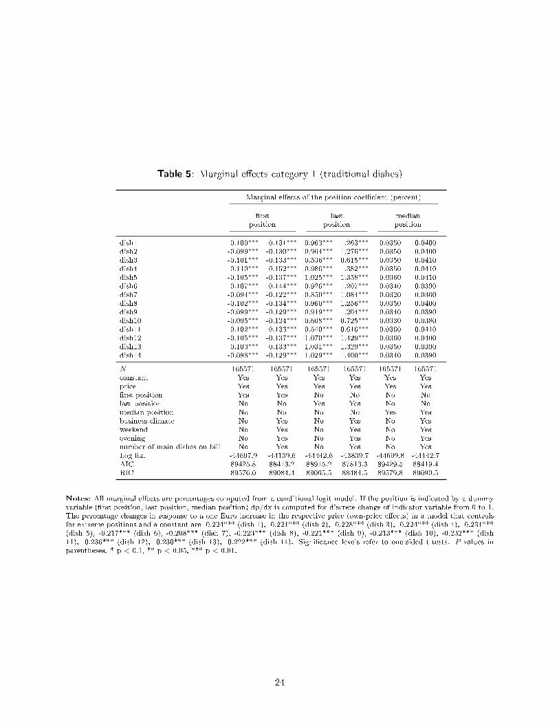
Table 5: Marginal e�ects category 1 (traditional dishes)

Marginal e�ects of the position coe�cient (percent)

�rst last medianposition position position

dish1 -0.100∗∗∗ -0.131∗∗∗ 0.963∗∗∗ 1.263∗∗∗ 0.0350 0.0400dish2 -0.099∗∗∗ -0.130∗∗∗ 0.964∗∗∗ 1.276∗∗∗ 0.0350 0.0400dish3 -0.101∗∗∗ -0.133∗∗∗ 0.536∗∗∗ 0.615∗∗∗ 0.0350 0.0410dish4 -0.110∗∗∗ -0.152∗∗∗ 0.986∗∗∗ 1.382∗∗∗ 0.0350 0.0410dish5 -0.105∗∗∗ -0.137∗∗∗ 1.025∗∗∗ 1.358∗∗∗ 0.0360 0.0410dish6 -0.107∗∗∗ -0.144∗∗∗ 0.926∗∗∗ 1.207∗∗∗ 0.0340 0.0390dish7 -0.094∗∗∗ -0.122∗∗∗ 0.850∗∗∗ 1.084∗∗∗ 0.0320 0.0360dish8 -0.102∗∗∗ -0.134∗∗∗ 0.960∗∗∗ 1.256∗∗∗ 0.0350 0.0400dish9 -0.099∗∗∗ -0.129∗∗∗ 0.919∗∗∗ 1.204∗∗∗ 0.0340 0.0390dish10 -0.095∗∗∗ -0.124∗∗∗ 0.608∗∗∗ 0.725∗∗∗ 0.0330 0.0380dish11 -0.102∗∗∗ -0.133∗∗∗ 0.540∗∗∗ 0.616∗∗∗ 0.0360 0.0410dish12 -0.105∗∗∗ -0.137∗∗∗ 1.070∗∗∗ 1.429∗∗∗ 0.0360 0.0400dish13 -0.103∗∗∗ -0.133∗∗∗ 1.031∗∗∗ 1.329∗∗∗ 0.0350 0.0390dish14 -0.098∗∗∗ -0.129∗∗∗ 1.029∗∗∗ 1.400∗∗∗ 0.0340 0.0390

N 165571 165571 165571 165571 165571 165571constant Yes Yes Yes Yes Yes Yesprice Yes Yes Yes Yes Yes Yes�rst position Yes Yes No No No Nolast position No No Yes Yes No Nomedian position No No No No Yes Yesbusiness climate No Yes No Yes No Yesweekend No Yes No Yes No Yesevening No Yes No Yes No Yesnumber of main dishes on bill No Yes No Yes No YesLog lik. -44697.9 -44139.6 -44442.6 -43839.7 -44699.8 -44142.7AIC 89425.8 88413.2 88915.2 87813.3 89429.5 88419.4BIC 89576.0 89084.4 89065.5 88484.5 89579.8 89090.5

Notes: All marginal e�ects are percentages computed from a conditional logit model. If the position is indicated by a dummyvariable (�rst position, last position, median position) dp/dx is computed for discrete change of indicator variable from 0 to 1.The percentage changes in response to a one Euro increase in the respective price (own-price e�ects) in a model that controlsfor extreme positions and a constant are -0.224*** (dish 1), -0.221*** (dish 2), -0.228*** (dish 3), -0.224*** (dish 4), -0.231***(dish 5), -0.217*** (dish 6), -0.208*** (dish 7), -0.223*** (dish 8), -0.221*** (dish 9), -0.213*** (dish 10), -0.232*** (dish11), -0.236*** (dish 12), -0.230*** (dish 13), -0.222*** (dish 14). Signi�cance levels refer to one-sided t-tests. P -values inparentheses. * p < 0.1, ** p < 0.05, *** p < 0.01.

24

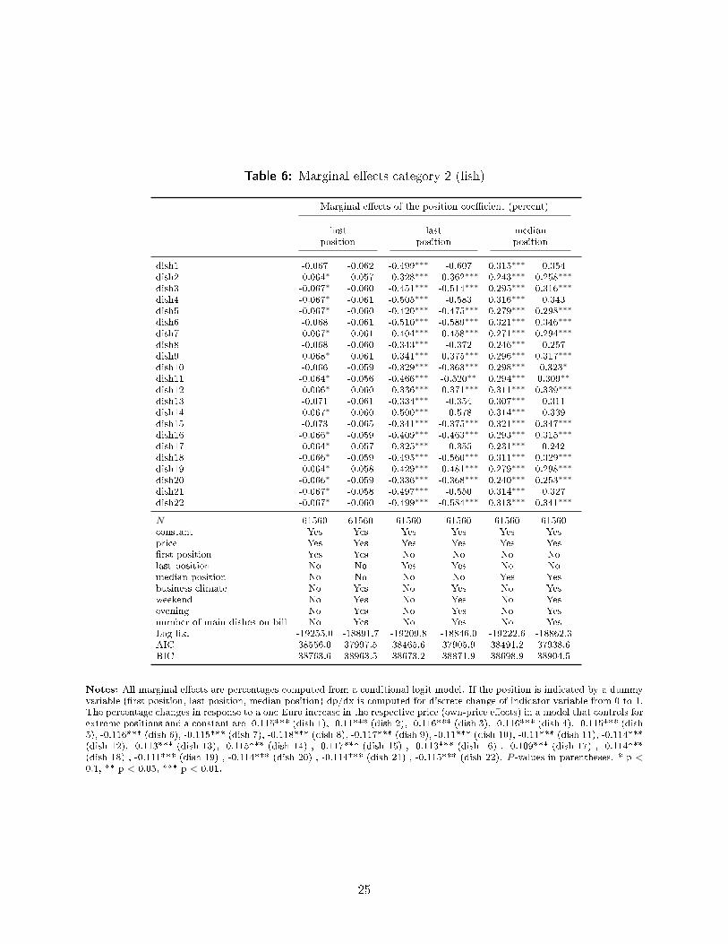
Table 6: Marginal e�ects category 2 (�sh)



dish1 -0.067 -0.062 -0.499∗∗∗ -0.607 0.315∗∗∗ 0.354dish2 -0.064∗ -0.057 -0.328∗∗∗ -0.362∗∗∗ 0.243∗∗∗ 0.258∗∗∗

dish3 -0.067∗ -0.060 -0.451∗∗∗ -0.514∗∗∗ 0.295∗∗∗ 0.316∗∗∗

dish4 -0.067∗ -0.061 -0.505∗∗∗ -0.583 0.316∗∗∗ 0.343dish5 -0.067∗ -0.060 -0.420∗∗∗ -0.475∗∗∗ 0.279∗∗∗ 0.298∗∗∗

dish6 -0.068 -0.061 -0.510∗∗∗ -0.589∗∗∗ 0.321∗∗∗ 0.346∗∗∗

dish7 -0.067∗ -0.061 -0.404∗∗∗ -0.458∗∗∗ 0.271∗∗∗ 0.294∗∗∗

dish8 -0.068 -0.060 -0.343∗∗∗ -0.372 0.246∗∗∗ 0.257dish9 -0.068∗ -0.061 -0.341∗∗∗ -0.375∗∗∗ 0.296∗∗∗ 0.317∗∗∗

dish10 -0.066 -0.059 -0.329∗∗∗ -0.363∗∗∗ 0.298∗∗∗ 0.323∗

dish11 -0.064∗ -0.056 -0.466∗∗∗ -0.520∗∗ 0.294∗∗∗ 0.309∗∗

dish12 -0.066∗ -0.060 -0.336∗∗∗ -0.371∗∗∗ 0.311∗∗∗ 0.339∗∗∗

dish13 -0.071 -0.061 -0.334∗∗∗ -0.354 0.307∗∗∗ 0.311dish14 -0.067∗ -0.060 -0.500∗∗∗ -0.578 0.314∗∗∗ 0.339dish15 -0.073 -0.065 -0.341∗∗∗ -0.375∗∗∗ 0.321∗∗∗ 0.347∗∗∗

dish16 -0.066∗ -0.059 -0.409∗∗∗ -0.463∗∗∗ 0.293∗∗∗ 0.315∗∗∗

dish17 -0.064∗ -0.057 -0.325∗∗∗ -0.355 0.231∗∗∗ 0.242dish18 -0.066∗ -0.059 -0.495∗∗∗ -0.560∗∗∗ 0.311∗∗∗ 0.329∗∗∗

dish19 -0.064∗ -0.058 -0.429∗∗∗ -0.481∗∗∗ 0.279∗∗∗ 0.298∗∗∗

dish20 -0.066∗ -0.059 -0.336∗∗∗ -0.368∗∗∗ 0.240∗∗∗ 0.253∗∗∗

dish21 -0.067∗ -0.058 -0.497∗∗∗ -0.550 0.314∗∗∗ 0.327dish22 -0.067∗ -0.060 -0.499∗∗∗ -0.584∗∗∗ 0.313∗∗∗ 0.341∗∗∗


Notes: All marginal e�ects are percentages computed from a conditional logit model. If the position is indicated by a dummyvariable (�rst position, last position, median position) dp/dx is computed for discrete change of indicator variable from 0 to 1.The percentage changes in response to a one Euro increase in the respective price (own-price e�ects) in a model that controls forextreme positions and a constant are -0.115*** (dish 1), -0.11*** (dish 2), -0.116*** (dish 3), -0.116*** (dish 4), -0.115*** (dish5), -0.116*** (dish 6), -0.115*** (dish 7), -0.118*** (dish 8), -0.117*** (dish 9), -0.11*** (dish 10), -0.11*** (dish 11), -0.114***(dish 12), -0.113*** (dish 13), -0.115*** (dish 14) , -0.117*** (dish 15) , -0.113*** (dish 16) , -0.109*** (dish 17) , -0.114***(dish 18) , -0.111*** (dish 19) , -0.114*** (dish 20) , -0.114*** (dish 21) , -0.115*** (dish 22). P -values in parentheses. * p <0.1, ** p < 0.05, *** p < 0.01.

25

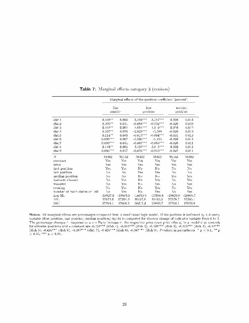
Table 7: Marginal e�ects category 3 (venison)



dish1 0.108∗∗ 0.066 -3.139∗∗∗ -3.547∗∗∗ -0.029 0.013dish2 0.093∗∗ 0.054 -0.858∗∗∗ -0.922∗∗∗ -0.026 0.010dish3 0.102∗∗ 0.061 -1.691∗∗∗ -1.919∗∗∗ -0.028 0.012dish4 0.107∗∗ 0.070 -2.823∗∗∗ -5.569 -0.029 0.013dish5 0.114∗∗ 0.069 -0.815∗∗∗ -0.864∗∗∗ -0.031 0.013dish6 0.099∗∗∗ 0.067 -1.006∗∗∗ -1.155 -0.029 0.014dish7 0.090∗∗∗ 0.054 -0.807∗∗∗ -0.863∗∗∗ -0.026 0.011dish8 0.110∗∗ 0.065 -3.132∗∗∗ -3.813∗∗∗ -0.030 0.013dish9 0.096∗∗∗ 0.057 -0.876∗∗∗ -0.943∗∗∗ -0.027 0.011


Notes: All marginal e�ects are percentages computed from a conditional logit model. If the position is indicated by a dummyvariable (�rst position, last position, median position) dp/dx is computed for discrete change of indicator variable from 0 to 1.The percentage changes in response to a one Euro increase in the respective price (own-price e�ects) in a model that controlsfor extreme positions and a constant are -0.424*** (dish 1), -0.364*** (dish 2), -0.409*** (dish 3), -0.415*** (dish 4), -0.44***(dish 5), -0.424*** (dish 6), -0.387*** (dish 7), -0.426*** (dish 8), -0.387*** (dish 9). P -values in parentheses. * p < 0.1, ** p< 0.05, *** p < 0.01.

26

Table 8: Marginal e�ects category 4 (steaks)



dish1 -0.835∗∗∗ -0.752∗∗∗ -0.025 -0.00800 0.093∗∗∗ 0.093∗∗∗

dish2 -0.829∗∗∗ -0.743∗∗∗ -0.024 -0.00700 0.090∗∗∗ 0.088∗∗∗

dish3 -0.850∗∗∗ -0.772∗∗∗ -0.029 -0.00800 0.114∗∗∗ 0.112∗∗∗

dish4 -0.833∗∗∗ -0.750∗∗∗ -0.025 -0.00700 0.097∗∗∗ 0.095∗∗∗

dish5 -0.817∗∗∗ -0.727∗∗∗ -0.022 -0.00700 0.085∗∗∗ 0.083∗∗∗

dish6 -2.454∗∗∗ -1.870∗∗∗ -0.025 -0.00700 0.098∗∗∗ 0.098∗∗∗

N 86387 86387 86387 86387 86387 86387constant Yes Yes Yes Yes Yes Yesprice Yes Yes Yes Yes Yes Yes�rst position Yes Yes No No No Nolast position No No Yes Yes No Nomedian position No No No No Yes Yesbusiness climate No No No Yes No Yesweekend No Yes No Yes No Yesevening No Yes No Yes No Yesnumber of main dishes on bill No Yes No Yes No YesLog lik. -27000.3 -26655.3 -26999.6 -26654.4 -26991.5 -26647.7AIC 54012.5 53362.7 54013.2 53362.8 53997.1 53349.3BIC 54068.7 53606.2 54078.8 53615.7 54062.7 53602.2

Notes: All marginal e�ects are percentages computed from a conditional logit model. Estimates displayed in columns 1 and2 have to be interpreted with caution because the likelihood is not globally concave (too little variation in the data). If theposition is indicated by a dummy variable (�rst position, last position, median position) dp/dx is computed for discrete changeof indicator variable from 0 to 1. The percentage changes in response to a one Euro increase in the respective price (own-pricee�ects) in a model that controls for extreme positions and a constant are -0.329*** (dish 1), -0.315*** (dish 2), -0.367*** (dish3), -0.324*** (dish 4), -0.29*** (dish 5), -0.323*** (dish 6). P -values in parentheses. * p < 0.1, ** p < 0.05, *** p < 0.01.

27

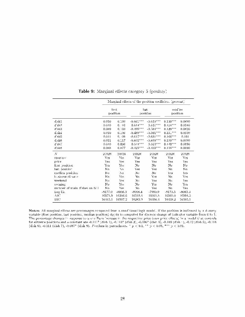
Table 9: Marginal e�ects category 5 (poultry)



dish1 0.010 0.109 -0.601∗∗∗ -0.619∗∗∗ 0.139∗∗∗ 0.0880dish2 0.010 0.110 -0.814∗∗∗ -0.837∗∗∗ 0.154∗∗∗ 0.0940dish3 0.009 0.103 -0.495∗∗∗ -0.504∗∗∗ 0.129∗∗∗ 0.0820dish4 0.010 0.100 -0.489∗∗∗ -0.501∗∗∗ 0.151∗∗∗ 0.0930dish5 0.011 0.109 -0.617∗∗∗ -0.631∗∗∗ 0.166∗∗∗ 0.101dish6 0.011 0.117 -0.832∗∗∗ -0.858∗∗∗ 0.159∗∗∗ 0.0980dish7 0.010 0.096 -0.544∗∗∗ -0.553∗∗∗ 0.148∗∗∗ 0.0890dish8 0.008 0.077 -0.423∗∗∗ -0.430∗∗∗ 0.116∗∗∗ 0.0690


Notes: All marginal e�ects are percentages computed from a conditional logit model. If the position is indicated by a dummyvariable (�rst position, last position, median position) dp/dx is computed for discrete change of indicator variable from 0 to 1.The percentage changes in response to a one Euro increase in the respective price (own-price e�ects) in a model that controlsfor extreme positions and a constant are -0.111* (dish 1), -0.113* (dish 2), -0.106* (dish 3), -0.109 (dish 4), -0.12 (dish 5), -0.118(dish 6), -0.111 (dish 7), -0.087* (dish 8). P -values in parentheses. * p < 0.1, ** p < 0.05, *** p < 0.01.

28

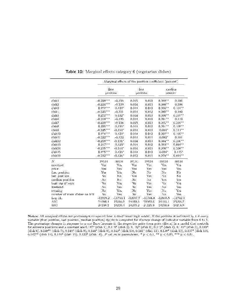
Table 10: Marginal e�ects category 6 (vegetarian dishes)



dish1 -0.229∗∗∗ -0.138 0.015 0.013 0.088∗∗ 0.106dish2 -0.224∗∗∗ -0.139 0.014 0.013 0.086∗∗ 0.106dish3 -0.222∗∗∗ -0.132∗ 0.014 0.013 0.086∗∗ 0.101∗∗

dish4 -0.223∗∗∗ -0.131 0.014 0.012 0.085∗∗ 0.100dish5 -0.222∗∗∗ -0.132∗ 0.014 0.013 0.090∗∗ 0.107∗∗

dish6 -0.219∗∗∗ -0.139 0.014 0.013 0.091∗∗ 0.119dish7 -0.229∗∗∗ -0.138 0.015 0.013 0.091∗∗ 0.109∗∗

dish8 -0.235∗∗∗ -0.135∗ 0.014 0.012 0.091∗∗ 0.108∗∗

dish9 -0.225∗∗∗ -0.134∗ 0.014 0.013 0.094∗ 0.114∗∗

dish10 -0.224∗∗∗ -0.132∗ 0.014 0.013 0.092∗∗ 0.109∗∗

dish11 -0.222∗∗∗ -0.122 0.014 0.011 0.092∗ 0.101dish12 -0.218∗∗∗ -0.131∗ 0.014 0.013 0.084∗∗ 0.100∗∗

dish13 -0.217∗∗∗ -0.123∗ 0.014 0.012 0.083∗∗ 0.094∗∗

dish14 -0.255∗∗∗ -0.144∗ 0.014 0.013 0.090∗∗ 0.108∗∗

dish15 -0.225∗∗∗ -0.135∗ 0.014 0.013 0.094∗ 0.115∗

dish16 -0.232∗∗∗ -0.126∗ 0.012 0.011 0.079∗∗ 0.094∗∗


Notes: All marginal e�ects are percentages computed from a conditional logit model. If the position is indicated by a dummyvariable (�rst position, last position, median position) dp/dx is computed for discrete change of indicator variable from 0 to 1.The percentage changes in response to a one Euro increase in the respective price (own-price e�ects) in a model that controlsfor extreme positions and a constant are 0.147* (dish 1), 0.143* (dish 2), 0.142* (dish 3), 0.142* (dish 4), 0.141* (dish 5), 0.139*(dish 6), 0.148** (dish 7), 0.140* (dish 8), 0.144* (dish 9), 0.143* (dish 10), 0.141* (dish 11), 0.138* (dish 12), 0.137* (dish 13),0.142** (dish 14), 0.144* (dish 15), 0.122* (dish 16). P -values in parentheses. * p < 0.1, ** p < 0.05, *** p < 0.01.

29

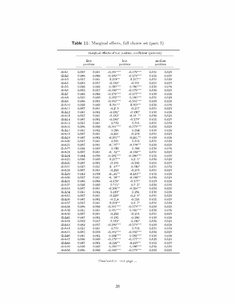
Table 11: Marginal e�ects, full choice set (part 1)



dish1 0.067 0.061 -0.181∗∗∗ -0.179∗∗∗ 0.031 0.029dish2 0.066 0.060 -0.180∗∗∗ -0.179∗∗∗ 0.031 0.029dish3 0.067 0.061 -0.219∗∗ -0.217∗∗ 0.031 0.029dish4 0.063 0.057 -0.183∗ -0.181 0.031 0.029dish5 0.066 0.060 -0.182∗∗∗ -0.180∗∗∗ 0.030 0.028dish6 0.062 0.057 -0.180∗∗∗ -0.179∗∗∗ 0.030 0.028dish7 0.066 0.060 -0.179∗∗∗ -0.177∗∗∗ 0.030 0.028dish8 0.065 0.060 -0.182∗∗∗ -0.180∗∗∗ 0.031 0.029dish9 0.066 0.061 -0.183∗∗∗ -0.181∗∗∗ 0.030 0.028dish10 0.066 0.060 -0.204∗∗ -0.202∗∗ 0.030 0.028dish11 0.067 0.061 -0.219 -0.217 0.031 0.029dish12 0.067 0.061 -0.181∗ -0.180∗ 0.030 0.028dish13 0.067 0.061 -0.182∗ -0.181∗∗ 0.030 0.028dish14 0.067 0.061 -0.180∗ -0.179∗ 0.031 0.029dish15 0.067 0.061 -0.220 -0.218 0.031 0.029dish16 0.066 0.060 -0.181∗∗∗ -0.179∗∗∗ 0.030 0.028dish17 0.067 0.061 -0.206 -0.204 0.030 0.029dish18 0.067 0.061 -0.221 -0.219 0.031 0.029dish19 0.067 0.061 -0.203∗∗ -0.201∗∗ 0.030 0.028dish20 0.067 0.061 -0.221 -0.219 0.031 0.029dish21 0.067 0.061 -0.197∗∗ -0.196∗∗ 0.030 0.028dish22 0.068 0.062 -0.186 -0.184 0.030 0.028dish23 0.067 0.061 -0.182∗∗ -0.180∗∗ 0.031 0.029dish24 0.064 0.059 -0.181∗∗∗ -0.180∗∗∗ 0.031 0.029dish25 0.066 0.060 -0.217∗∗ -0.215∗ 0.030 0.029dish26 0.067 0.061 -0.181 -0.180 0.031 0.029dish27 0.062 0.057 -0.182∗∗ -0.180∗ 0.031 0.029dish28 0.067 0.061 -0.220 -0.219 0.031 0.029dish29 0.063 0.058 -0.185∗∗ -0.183∗∗ 0.031 0.029dish30 0.067 0.061 -0.198∗∗ -0.196∗∗ 0.030 0.028dish31 0.066 0.060 -0.178∗ -0.177∗ 0.029 0.028dish32 0.066 0.060 -0.215∗ -0.213∗ 0.030 0.028dish33 0.067 0.061 -0.206∗∗ -0.204∗∗ 0.030 0.028dish34 0.067 0.061 -0.183∗ -0.181 0.030 0.028dish35 0.067 0.061 -0.220∗ -0.218∗ 0.031 0.029dish36 0.067 0.061 -0.218 -0.216 0.031 0.029dish37 0.067 0.061 -0.219∗∗ -0.217∗ 0.031 0.029dish38 0.066 0.060 -0.181∗∗∗ -0.179∗∗∗ 0.030 0.028dish39 0.067 0.061 -0.197∗∗∗ -0.195∗∗∗ 0.030 0.028dish40 0.067 0.061 -0.220 -0.218 0.031 0.029dish41 0.067 0.061 -0.181 -0.180 0.030 0.028dish42 0.062 0.057 -0.182∗ -0.180∗ 0.030 0.028dish43 0.062 0.057 -0.180∗∗∗ -0.179∗∗∗ 0.030 0.028dish44 0.067 0.061 -0.221 -0.219 0.031 0.029dish45 0.065 0.059 -0.182∗∗∗ -0.180∗∗∗ 0.030 0.028dish46 0.067 0.061 -0.184∗∗∗ -0.182∗∗∗ 0.030 0.028dish47 0.066 0.060 -0.179∗∗∗ -0.177∗∗∗ 0.029 0.028dish48 0.067 0.061 -0.220∗∗ -0.218∗∗ 0.031 0.029dish49 0.066 0.060 -0.188∗∗∗ -0.186∗∗∗ 0.030 0.028dish50 0.066 0.060 -0.180∗∗∗ -0.179∗∗∗ 0.030 0.028

Continued on next page ...

30

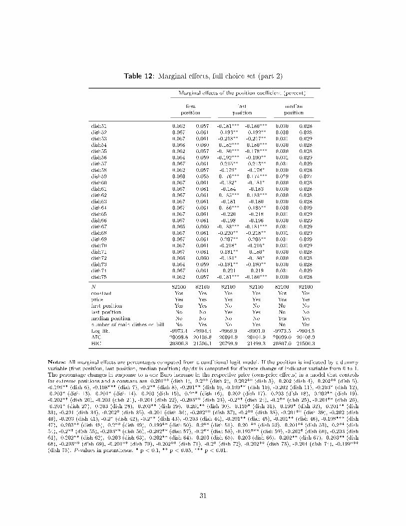
Table 12: Marginal e�ects, full choice set (part 2)



dish51 0.062 0.057 -0.181∗∗∗ -0.180∗∗∗ 0.030 0.028dish52 0.067 0.061 -0.193∗∗ -0.192∗∗ 0.030 0.028dish53 0.067 0.061 -0.218∗∗ -0.217∗∗ 0.031 0.029dish54 0.066 0.060 -0.182∗∗∗ -0.180∗∗∗ 0.030 0.028dish55 0.062 0.057 -0.180∗∗∗ -0.178∗∗∗ 0.030 0.028dish56 0.064 0.059 -0.192∗∗∗ -0.190∗∗ 0.031 0.029dish57 0.067 0.061 -0.215∗∗ -0.213∗∗ 0.031 0.029dish58 0.062 0.057 -0.179∗ -0.178∗ 0.030 0.028dish59 0.060 0.055 -0.176∗∗∗ -0.174∗∗∗ 0.029 0.027dish60 0.067 0.061 -0.182∗ -0.181∗ 0.030 0.028dish61 0.067 0.061 -0.184 -0.183 0.030 0.028dish62 0.067 0.061 -0.185∗∗∗ -0.183∗∗∗ 0.030 0.028dish63 0.067 0.061 -0.181 -0.180 0.030 0.028dish64 0.067 0.061 -0.186∗∗∗ -0.185∗∗ 0.030 0.029dish65 0.067 0.061 -0.220 -0.218 0.031 0.029dish66 0.067 0.061 -0.198 -0.196 0.030 0.029dish67 0.065 0.060 -0.183∗∗∗ -0.181∗∗∗ 0.031 0.029dish68 0.067 0.061 -0.220∗∗ -0.218∗∗ 0.031 0.029dish69 0.067 0.061 -0.207∗∗ -0.205∗∗ 0.031 0.029dish70 0.067 0.061 -0.218∗ -0.216∗ 0.031 0.029dish71 0.067 0.061 -0.181∗∗ -0.180∗ 0.030 0.028dish72 0.066 0.060 -0.181∗ -0.180∗ 0.030 0.028dish73 0.064 0.059 -0.181∗∗ -0.180∗∗ 0.030 0.028dish74 0.067 0.061 -0.221 -0.219 0.031 0.029dish75 0.062 0.057 -0.181∗∗∗ -0.180∗∗∗ 0.030 0.028

N 82100 82100 82100 82100 82100 82100constant Yes Yes Yes Yes Yes Yesprice Yes Yes Yes Yes Yes Yes�rst position Yes Yes No No No Nolast position No No Yes Yes No Nomedian position No No No No Yes Yesnumber of main dishes on bill No Yes No Yes No YesLog lik. -9973.4 -9904.4 -9969.9 -9901.0 -9973.5 -9904.5AIC 20098.8 20108.8 20091.9 20101.9 20099.0 20108.9BIC 20806.8 21506.1 20799.9 21499.3 20807.0 21506.3

Notes: All marginal e�ects are percentages computed from a conditional logit model. If the position is indicated by a dummyvariable (�rst position, last position, median position) dp/dx is computed for discrete change of indicator variable from 0 to 1.The percentage changes in response to a one Euro increase in the respective price (own-price e�ects) in a model that controlsfor extreme positions and a constant are -0.201** (dish 1), -0.2** (dish 2), -0.202** (dish 3), -0.202 (dish 4), -0.202** (dish 5),-0.199** (dish 6), -0.198*** (dish 7), -0.2** (dish 8), -0.201** (dish 9), -0.199** (dish 10), -0.202 (dish 11), -0.203* (dish 12),-0.203* (dish 13), -0.201* (dish 14), -0.203 (dish 15), -0.2** (dish 16), -0.202 (dish 17), -0.203 (dish 18), -0.202** (dish 19),-0.202** (dish 20), -0.203 (dish 21), -0.204 (dish 22), -0.203** (dish 23), -0.2** (dish 24), -0.2** (dish 25), -0.204** (dish 26),-0.201* (dish 27), -0.203 (dish 28), -0.203** (dish 29), -0.201** (dish 30), -0.199* (dish 31), -0.199* (dish 32), -0.201** (dish33), -0.201 (dish 34), -0.202* (dish 35), -0.201 (dish 36), -0.202** (dish 37), -0.2** (dish 38), -0.201** (dish 39), -0.202 (dish40), -0.203 (dish 41), -0.2* (dish 42), -0.2** (dish 43), -0.203 (dish 44), -0.201** (dish 45), -0.201** (dish 46), -0.198*** (dish47), -0.203** (dish 48), -0.2** (dish 49), -0.199** (dish 50), -0.2** (dish 51), -0.201** (dish 52), -0.201** (dish 53), -0.2** (dish54), -0.2** (dish 55), -0.203** (dish 56), -0.202** (dish 57), -0.2** (dish 58), -0.193*** (dish 59), -0.202* (dish 60), -0.203 (dish61), -0.202** (dish 62), -0.203 (dish 63), -0.202** (dish 64), -0.203 (dish 65), -0.203 (dish 66), -0.202** (dish 67), -0.203** (dish68), -0.203** (dish 69), -0.201** (dish 70), -0.202** (dish 71), -0.2* (dish 72), -0.202** (dish 73), -0.204 (dish 74), -0.199***(dish 75). P -values in parentheses. * p < 0.1, ** p < 0.05, *** p < 0.01.

31

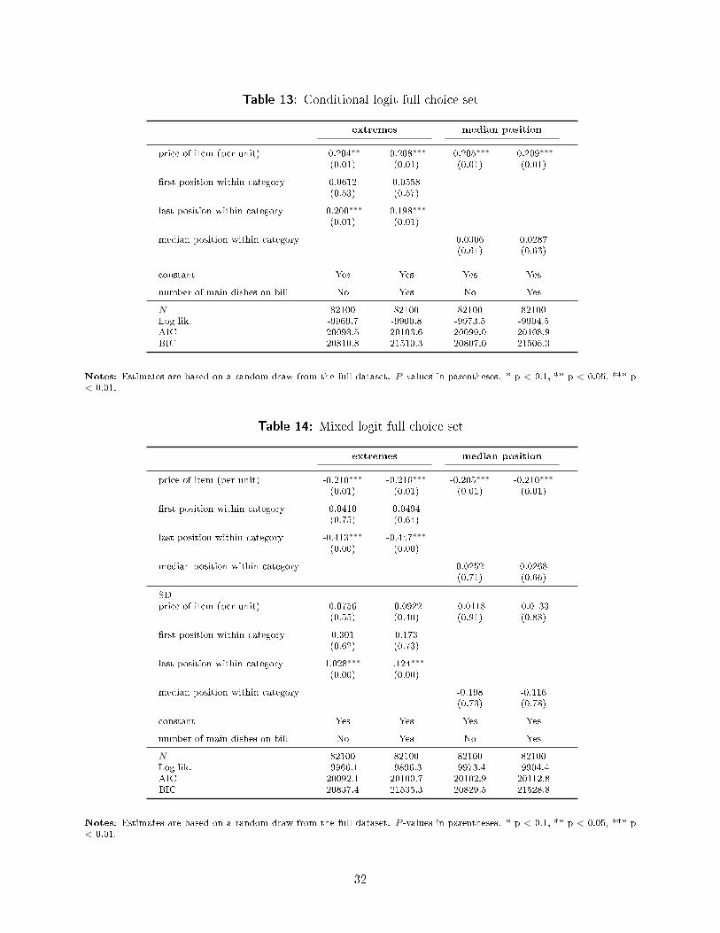
Table 13: Conditional logit full choice set

extremes median position

price of item (per unit) -0.204∗∗ -0.208∗∗∗ -0.205∗∗∗ -0.209∗∗∗

(0.01) (0.01) (0.01) (0.01)

�rst position within category 0.0612 0.0558(0.53) (0.57)

last position within category -0.200∗∗∗ -0.198∗∗∗

(0.01) (0.01)

median position within category 0.0306 0.0287(0.61) (0.63)

constant Yes Yes Yes Yes

number of main dishes on bill No Yes No Yes

N 82100 82100 82100 82100Log lik. -9969.7 -9900.8 -9973.5 -9904.5AIC 20093.5 20103.6 20099.0 20108.9BIC 20810.8 21510.3 20807.0 21506.3

Notes: Estimates are based on a random draw from the full dataset. P -values in parentheses. * p < 0.1, ** p < 0.05, *** p< 0.01.

Table 14: Mixed logit full choice set

extremes median position

price of item (per unit) -0.210∗∗∗ -0.216∗∗∗ -0.205∗∗∗ -0.210∗∗∗

(0.01) (0.01) (0.01) (0.01)



(0.00) (0.00)


SDprice of item (per unit) 0.0756 -0.0922 -0.0118 -0.0133

(0.55) (0.40) (0.91) (0.88)


last position within category 1.028∗∗∗ 1.124∗∗∗

(0.00) (0.00)

median position within category -0.198 -0.116(0.73) (0.78)


number of main dishes on bill No Yes No Yes

N 82100 82100 82100 82100Log lik. -9966.1 -9896.3 -9973.4 -9904.4AIC 20092.1 20100.7 20102.9 20112.8BIC 20837.4 21535.3 20829.5 21528.8

Notes: Estimates are based on a random draw from the full dataset. P -values in parentheses. * p < 0.1, ** p < 0.05, *** p< 0.01.

32

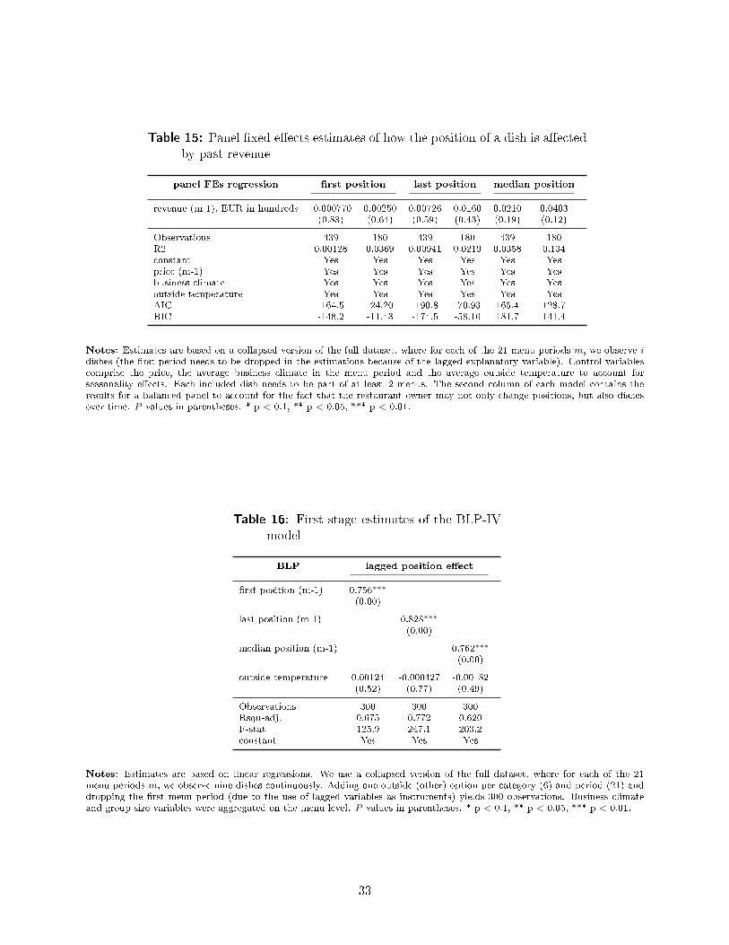
Table 15: Panel �xed e�ects estimates of how the position of a dish is a�ectedby past revenue

panel FEs regression �rst position last position median position

revenue (m-1), EUR in hundreds -0.000770 0.00250 0.00726 0.0160 0.0210 0.0403(0.83) (0.64) (0.59) (0.43) (0.19) (0.12)

Observations 439 180 439 180 439 180R2 0.00128 0.0369 0.00941 0.0219 0.0358 0.134constant Yes Yes Yes Yes Yes Yesprice (m-1) Yes Yes Yes Yes Yes Yesbusiness climate Yes Yes Yes Yes Yes Yesoutside temperature Yes Yes Yes Yes Yes YesAIC -164.5 -24.20 -190.8 -70.93 165.4 128.7BIC -148.2 -11.43 -174.5 -58.16 181.7 141.4

Notes: Estimates are based on a collapsed version of the full dataset, where for each of the 21 menu periods m, we observe idishes (the �rst period needs to be dropped in the estimations because of the lagged explanatory variable). Control variablescomprise the price, the average business climate in the menu period and the average outside temperature to account forseasonality e�ects. Each included dish needs to be part of at least 2 menus. The second column of each model contains theresults for a balanced panel to account for the fact that the restaurant owner may not only change positions, but also dishesover time. P -values in parentheses. * p < 0.1, ** p < 0.05, *** p < 0.01.

Table 16: First stage estimates of the BLP-IVmodel

BLP lagged position e�ect

�rst position (m-1) 0.756∗∗∗

(0.00)

last position (m-1) 0.828∗∗∗

(0.00)

median position (m-1) 0.762∗∗∗

(0.00)

outside temperature 0.00124 -0.000427 -0.00182(0.52) (0.77) (0.49)

Observations 300 300 300Rsqu-adj. 0.675 0.772 0.620F-stat 125.9 247.1 203.2constant Yes Yes Yes

Notes: Estimates are based on linear regressions. We use a collapsed version of the full dataset, where for each of the 21menu periods m, we observe nine dishes continuously. Adding one outside (other) option per category (6) and period (21) anddropping the �rst menu period (due to the use of lagged variables as instruments) yields 300 observations. Business climateand group size variables were aggregated on the menu level. P -values in parentheses. * p < 0.1, ** p < 0.05, *** p < 0.01.

33

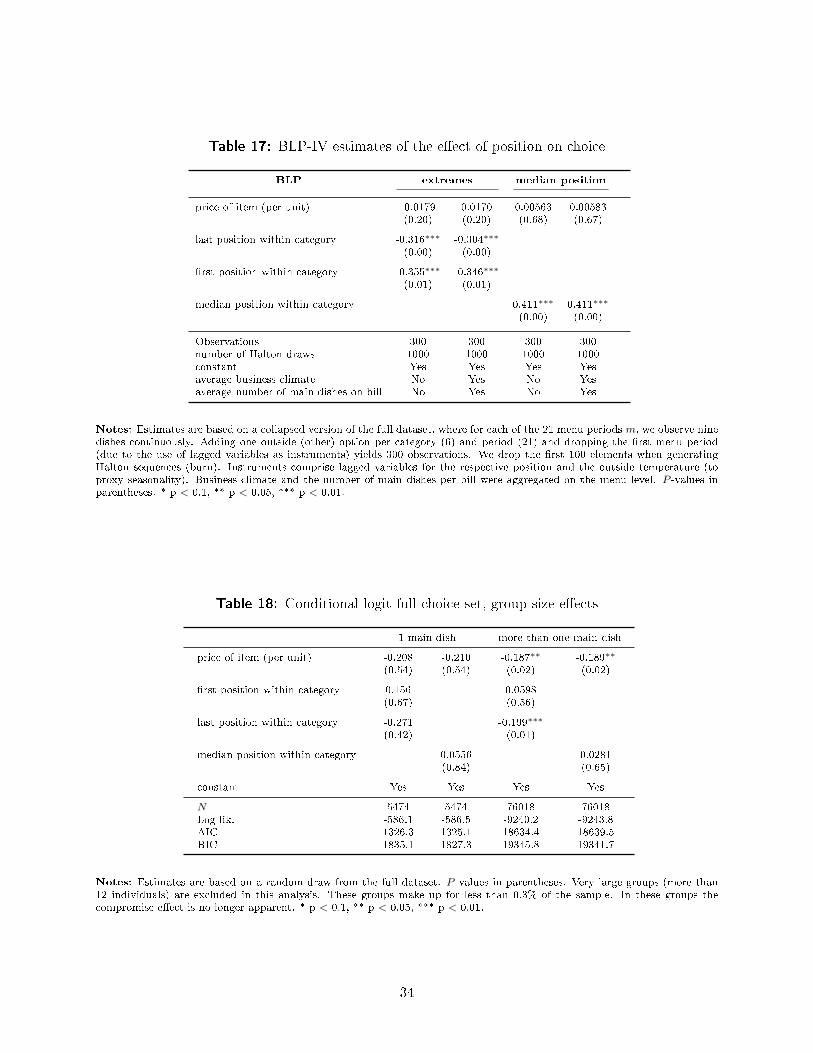
Table 17: BLP-IV estimates of the e�ect of position on choice

BLP extremes median position

price of item (per unit) -0.0179 0.0170 0.00563 0.00583(0.20) (0.20) (0.68) (0.67)


(0.00) (0.00)

�rst position within category -0.355∗∗∗ -0.346∗∗∗

(0.01) (0.01)

median position within category 0.411∗∗∗ 0.411∗∗∗

(0.00) (0.00)

Observations 300 300 300 300number of Halton draws 1000 1000 1000 1000constant Yes Yes Yes Yesaverage business climate No Yes No Yesaverage number of main dishes on bill No Yes No Yes

Notes: Estimates are based on a collapsed version of the full dataset, where for each of the 21 menu periods m, we observe ninedishes continuously. Adding one outside (other) option per category (6) and period (21) and dropping the �rst menu period(due to the use of lagged variables as instruments) yields 300 observations. We drop the �rst 100 elements when generatingHalton sequences (burn). Instruments comprise lagged variables for the respective position and the outside temperature (toproxy seasonality). Business climate and the number of main dishes per bill were aggregated on the menu level. P -values inparentheses. * p < 0.1, ** p < 0.05, *** p < 0.01.

Table 18: Conditional logit full choice set, group size e�ects

1 main dish more than one main dish

price of item (per unit) -0.208 -0.210 -0.187∗∗ -0.189∗∗

(0.54) (0.54) (0.02) (0.02)


last position within category -0.271 -0.199∗∗∗

(0.42) (0.01)



N 5474 5474 76018 76018Log lik. -586.1 -586.5 -9240.2 -9243.8AIC 1326.3 1325.1 18634.4 18639.5BIC 1835.1 1827.3 19345.8 19341.7

Notes: Estimates are based on a random draw from the full dataset. P -values in parentheses. Very large groups (more than12 individuals) are excluded in this analysis. These groups make up for less than 0.3% of the sample. In these groups thecompromise e�ect is no longer apparent. * p < 0.1, ** p < 0.05, *** p < 0.01.

34

the compromise effect in action: lessons from a restaurant ...ftp.iza.org/dp9648.pdf · iza...

Documents